1

INDIVIDUAL EXPOSURE TO TRAFFIC RELATED AIR POLLUTION

ACROSS LAND-USE CLUSTERS

Maryam Shekarrizfard

Doctoral Candidate

Department of Civil Engineering and Applied Mechanics, McGill University

817 Sherbrooke St. W., Room 492

Montréal, Québec, H3A 2K6, Canada

Tel: 1-514-589-4353, Fax: 1-514-398-7361

Email: maryam.shekarrizfard@mail.mcgill.ca

Ahmadreza Faghih-Imani

Doctoral Candidate

Department of Civil Engineering and Applied Mechanics, McGill University

817 Sherbrooke St. W., Room 492

Montréal, Québec, H3A 2K6, Canada

Tel: 1-514-589-4353, Fax: 1-514-398-7361

Email: seyed.faghihimani@mail.mcgill.ca

Dan L Crouse, PhD

Research Associate

Department of Sociology, University of New Brunswick

New Brunswick, Canada

Email: dlcrouse@gmail.com

Mark Goldberg, PhD

Professor

Department of Medicine, McGill University

Division of Clinical Epidemiology, McGill University Health Centre, QC H3A 1A1, Canada

Tel: 1-514-934-1934, ext 36917; Fax: 1-514-843-1493

Email: mark.goldberg@mcgill.ca

Nancy Ross, PhD

Associate Professor, Department of Geography

Associate, Department of Epidemiology and Biostatistics

McGill University

805 Sherbrooke St. W., Montreal, Quebec H3A 2K6

Tel: 1-514-398-4307 Fax: 1-514-398-3747

Email: nancy.ross@mcgill.ca

Naveen Eluru

Associate Professor

Department of Civil, Environmental and Construction Engineering, University of Central Florida

12800 Pegasus Drive, Room 301D

Orlando, Florida 32816, USA

Tel.: 407-823-4815; Fax: 407-823-3315

Email: naveen.eluru@ucf.edu

Marianne Hatzopoulou (corresponding Author)

Associate Professor

Department of Civil Engineering, University of Toronto

35 St George Street, Toronto, ON M5S 1A4

Tel:1- 416-978-0864 Fax: 1-416-978-6813

E-mail: marianne.hatzopoulou@utoronto.ca

2

INDIVIDUAL EXPOSURE TO TRAFFIC RELATED AIR POLLUTION

ACROSS LAND-USE CLUSTERS

ABSTRACT

In this study, we estimated the transportation-related emissions of nitrogen oxides (NOx) at an

individual level for a sample of the Montreal population. Using linear regression, we quantified

the associations between NOx emissions and selected individual attributes. We then investigated

the relationship between individual emissions of NOx and exposure to nitrogen dioxide (NO2)

concentrations derived from a land-use regression model. Factor analysis and clustering of land-

uses were used to test the relationships between emissions and exposures in different Montreal

areas. We observed that the emissions generated per individual are positively associated with

vehicle ownership, gender, and employment status. We also noted that individuals who live in the

suburbs or in peripheral areas generate higher emissions of NOx but are exposed to lower NO2

concentrations at home and throughout their daily activities. Finally, we observed that for most

individuals, NO2 exposures based on daily activity locations were often slightly more elevated

than NO2 concentrations at the home location. We estimated that between 20% and 45% of

individuals experience a daily exposure that is largely different from the concentration at their

home location. Our findings are relevant to the evaluation of equity in the generation of transport

emissions and exposure to traffic-related air pollution. We also shed light on the effect of

accounting for daily activities when estimating air pollution exposure.

Keywords: transport emissions, traffic related air pollution, exposure, land-use, built environment,

travel survey

3

1. INTRODUCTION

Transport plays a crucial role in urban development by providing access to education, markets,

employment, recreation, health care and other key services. Currently, 82% of Canadian

commuters drive to work while the remainder rely on public transit and active transportation

(Turcotte, 2011). In Canada, on-road traffic accounts for 19% of nitrogen oxide (NOx) emissions

and in Montreal, Canada’s second largest city, transportation accounts for 85% of NOx emissions (Brisset and Moorman, 2009; Statistics Canada, 2012). In urban areas, NOx often refers to NO and

NO2 since the contribution of other nitrogen oxides is minimal. NOx concentrations are often used

as a tracer of road traffic emissions (Lewne et al., 2004). NOx is always higher in the vicinity of

roadways and lower further away, as roads are the major source of NOx emissions. Meteorological

parameters such as wind speed and direction affect the decay of NOx concentrations away from

the roadway. Ambient nitrogen dioxide (NO2) is associated with vehicular traffic since vehicles

mostly emit NO, which is then transformed to NO2 through photochemical reactions involving

ozone and volatile organic compounds. However, because ambient NO2 is also affected by other

sources (such as industries), we would expect NO2 to have lower spatial variability compared to

NOx concentrations that would exhibit large differences between roadways and residential areas.

Gilbert et al. (2005) argue that more than 50% of the variability in air pollution concentrations in

Montreal can be explained by local traffic.

Exposure to traffic-related air pollution has been associated with various acute and chronic

health effects (Cesaroni et al., 2012; Crouse et al., 2010; Gan et al., 2012; Künzli et al., 2000;

Smargiassi et al., 2005). A number of studies have established positive associations between

various cancers and exposure to NO2 an accepted marker of traffic-related air pollution (Ahrens,

2003; Costa et al., 2014; Crouse et al., 2010; Parent et al., 2013; Snowden et al., 2014;

Shekarrizfard et al., 2015). Part of the challenge of reducing ambient air pollution in urban areas

involves reducing the demand for private motorized transportation at an individual and household

level. As such, there is a need for analysis tools that can assist policy-makers in evaluating the

impacts of transport policies on urban air quality and population exposure. Tools that can provide

detailed air emission estimates at a person and trip level are also of extreme relevance to the

appraisal of transport plans. Recently, a number of researchers developed modelling frameworks

that account for vehicle emissions whereby activity-based models were used to calculate person-

and trip-level emissions (Beckx et al., 2009a). A number of studies have also included an analysis

of atmospheric dispersion and population exposure (Beckx et al., 2009b; Hatzopoulou and Miller,

2010; Int Panis et al., 2011).

Travel activity, land use patterns, and the distribution of traffic often lead to inequities in

the exposure to vehicle-related air pollutants (Buzzelli and Jerrett, 2003, 2007; Houston et al.,

2004; Jerrett, 2009). Individuals who live in densely populated areas may be exposed to higher

concentrations while generating low levels of emissions throughout their daily travel (Dannenberg

et al., 2003). Most studies that examine the generation of transport-related emissions ignore their

effect on air quality and exposure, while studies that investigate exposure to air pollution rarely

investigate the generation of air emissions (Fallon, 2002; Hatzopoulou and Miller, 2010; Havard

et al., 2009; Sider et al., 2013).

In this paper we quantify the emissions of -and exposure to- traffic-related air pollution

simultaneously at an individual level. We hypothesize that high emitters would reside in areas

characterized by low air pollution (e.g. suburbs) while low emitters would reside in areas with

4

poor air quality (neighborhoods of the inner city). We also investigate the relationship between

both variables across different land-uses and socio-economic characteristics.

2. MATERIALS AND METHODS

Our methodology consists of three main steps: 1) generating individual-level NOx emissions from

daily travel using a traffic assignment model extended with detailed emission modelling capability,

2) estimating individual daily exposure to NO2 using a land-use regression model; and 3)

investigating the determinants of NOx emissions and the relationship with NO2 exposures as a

function of land-use and socio-demographic characteristics. Our study area is focused on the Island

of Montreal (Fig. 1).

2.1 Description of Data Sources

We estimated NOx emissions for car users using a transportation and emissions model. This model

includes a traffic assignment component linked with an emission tool that simulates traffic flows

and emissions for driving trips in the Montreal metropolitan region (Sider et al., 2013). The traffic

assignment model, which is developed in the PTV VISUM platform (Vision, 2009), simulates

traffic flow, average speed, and vehicle mix on every road segment and was validated against

traffic counts at several major intersections and bridges within the region (R2 = 0.65) (Sider et al.,

2013). Based on the vehicle mix per road segment, average speed, and type of roadway (e.g.

highway vs. arterial road with intersections), an emission factor for NOx was assigned to the road

segment. Emission Factors were derived from the MOtor Vehicle Emission Simulator (MOVES)

model, with input data describing local conditions (USEPA, 2013). After summarizing the daily

driving trips for each person in the origin-destination survey, NOx emissions were calculated for

each individual.

In addition to deriving individual NOx emissions from driving, we made use of estimates

of NO2 concentrations from a LUR model (Crouse et al., 2009), to generate a NO2 polygon-based

map (with gridcell dimensions 80m x 80m amounting to a total of approximately 60,000

polygons). This map (Fig. 2) was used to identify the NO2 concentration at the home location of

every individual as well as estimate daily exposures using data on activity locations using ESRI’s

ArcGIS. Since the NO2 estimates were derived from three separate 2-week sampling periods in

2006 thus representing a long-term average; we recognize that what we consider a daily exposure

is a weighted average NO2 concentration across daily activity locations (including home).

Therefore the spatial variability in NO2 concentrations is accounted for in the exposure metric but

not the temporal variability. Our activity-weighted NO2 concentration (in ppb) per person was

estimated using Equation (1).

m

k

k

stop

k

NOi

NOa

tCC

1 24

2

2

(1)

In Equation (1), m is number of trips for each individual (i), k

NOC

2

is the NO2 concentration

(in ppb) assigned to a destination using the NO2 polygon map, and k

stopt is the total time an

individual spent at every destination (in hours). We define the stop time ( k

stopt ) at each destination

5

as the difference between the start time of the trip leaving the activity location and the start time

of the trip leading to the activity. This means that the time spent on the trip leading to an activity

contributes to the exposure during that activity. We make this assumption to avoid calculating

exposures during travel. While we recognize this step as an approximation, it is made due to the

lack of information on in-vehicle exposures across modes.

While NOx emissions were generated for drivers only, daily NO2 exposures were compiled

for drivers and transit riders but not for those who took active transportation. This simplification

is due to the fact that we could not infer activity times associated with walking and cycling trips

due to the lack of paths and travel times for these trips. Future model developments will address

path selection and travel times for active transport users. We made use of the 2008 Origin-

Destination (O-D) survey for Montreal (AMT, 2010) to extract individual daily trip characteristics

including origin and destination coordinates, trip start time, mode and purpose, as well as

individual and household attributes (age, gender, employment status, household size, residential

location, and vehicle ownership). The OD survey includes information on a 5% sample of the

Montreal population, encompassing a total of 355,000 daily trips conducted by approximately

157,000 individuals associated with 66,000 households across the metropolitan region. We

restricted the data to the Island of Montreal (Fig. 1). Also, we considered only single mode trips,

thus yielding a final dataset of approximately 32,000 individuals. The latter restriction was needed

in order to facilitate the inference of trip paths and travel times across the road network.

Emissions and exposures were evaluated in the context of the residential location of

individuals in Montreal. For this purpose, we used factor analysis and clustering methods to

develop “land-use clusters” based on the 1,552 Traffic Analysis Zones (TAZs) in Montreal. The

geographic unit of analysis is the Traffic Analysis Zone (TAZ), a division used by the Québec

Ministry of Transportation (MTQ) in travel demand modelling and traffic assignment. A host of

variables were compiled at the TAZ level including: land-use variables (such as residential density,

commercial density, and governmental and institutional density), transportation network

characteristics (such as length of highways, minor roads, and major roads), public transit (bus stops

and metro stations), socio-economics (such as population density, job density, and average/median

income) and point of interests (such as restaurants, bars, and other commercial enterprises). All of

the variables mentioned were extracted from the Transportation Research at McGill (TRAM)

database: for the land use, point of interests and streets network, the DMTI Spatial Inc. Database

2009 was used, defining the road and land-use categories; the bus and metro stops are derived from

the local transit provider (STM 2010), the socio-economic data from Statistics Canada.

Due to the presence of a large number of variables that might be correlated with each other,

factor analysis was used to retrieve a smaller number of principal components. Then, a two-step

cluster analysis was used to classify each zone to be part of a cluster based on original variables

and derived components. Several possible loading configurations of variables for factor and cluster

analysis were used. Principal components estimation and varimax rotation were used in deriving

the results of factor analysis. Factor loadings below 0.20 were considered insignificant. Three

separate factors were identified for: 1) Public transport attributes 2) Road network attributes and

3) Points of interest attributes. Public transport attributes of a TAZ yielded two components

representing metro and bus service. The road network component captures transportation network

characteristics including the density of highways, major roads and local streets. The points of

interest factor encompasses the density of restaurants, bars and other commercial enterprises in a

zone.

6

2.2 Statistical Analysis

Our investigation addressed three different dimensions to the question of emission generation and

exposure at the individual level. First, we regressed the total NOx emissions generated by drivers

as a function of socio-economic variables. Second, we contrasted individual NOx emissions and

NO2 concentrations at the home location for these same individuals in order to investigate whether

“high emitters” resided in relatively low polluted areas. Finally, we examined whether average

NO2 concentrations at home locations were sufficient to understand daily exposures by contrasting

NO2 at home with daily activity-weighted NO2 exposures.

In order to identify the main variables associated with NOx emissions, we used a log-linear

multiple regression model to relate the logarithm of the generated emissions for drivers with

individual characteristics including employment status, gender, age, vehicle ownership, vehicle

type and age. We used an iterative process that allows dropping or adding variables. For this

purpose, we eliminated from the model the predictors one-by-one on the basis of their statistical

significance. The performance of the regression was evaluated using the root mean square error

(RMSE) and R2 of regression.

In order to compare daily NOx emissions from travel with NO2 concentrations at home

locations of the same individuals, we divided car users into four groups based on their home

location within one of the four land-use clusters that we identified in the cluster analysis. We

conducted a descriptive analysis to identify the clusters in terms of their contribution to traffic

emissions and air quality. In addition, we developed an exposure-emission index, which helped us

visualize the agreement between emissions and exposure (Equation 2). For example, this index

would represent whether those who emit a lot are also exposed to poor air quality at their home

location or whether they enjoy low concentrations of NO2 at home. For this purpose, we converted

NOx emissions and NO2 concentrations into deciles (with 1 indicating the lowest decile and 10 the

highest) and computed the ratio of NO2 to NOx (in deciles) at each TAZ. The ratio ranges from 0.1

representing minimum NO2 exposure and maximum NOx emissions to 10 representing maximum

NO2 exposure and minimum emissions (Equation 2).

Exposure to emission index= decileemission

decileexposure2

xNO

NO (2)

Finally, we conducted a comparison between daily activity-weighted NO2 exposure and

average NO2 concentration at the home location to evaluate the size of the discrepancy between

both measures. Traditional epidemiologic studies often rely on the air pollution concentration at

the home location as a potential predictor for the odds of various air pollution-related health effects

(Hamra et al., 2015; Lee et al., 2014; Parent et al., 2013; Chen et al., 2008; Krämer at al., 2000).

This dimension of our analysis investigates whether daily exposure can be approximated by the

daily average concentration at home. We conducted this analysis for both drivers and transit riders.

Moreover, we examined the frequencies of individuals for whom the differences between the

activity-weighted and at-home exposures are ‘large’ (i.e. those who accumulate in a day a lot more

or a lot less than the concentration at home). Our threshold for a ‘large’ difference is a difference

between an activity-weighted concentration and concentration at the home location that is 20

percent higher or lower than the mean difference for all individuals. The frequency of individuals

7

(f) with a ‘large’ difference is identified using Equations (3) and (4). We conducted this analysis

by land-use cluster and for car (j=1) and transit users (j=2) separately:

N

C

f

N

i

i

NOaCC

j

1

],[)(1

1

2maxmin

j=1, 2 (3)

0

1)(1

2maxmin ],[

i

NOaCCC

otherwise

CCCCCNOhNOh

i

NOaNOhNOh 22222

(4)

In Equation (3), N is the number of individuals in each cluster, i

NOaC

2 (in ppb) represents

the activity-weighted NO2 exposure and )(12maxmin ],[

i

NOaCCC

is an indicator function of the home-

NO2 exposure (2NOh

C ) which is defined in Equation (4) and based on (Ganji, 2010). In Equation

(4), is equal to 0.2 (indicating our threshold of 20%) and 2NOh

C represents the mean at-home

concentration for all individuals in a given cluster.

3. RESULTS AND DISCUSSION

3.1 Land-Use Clusters

The Montreal region consists of 1552 Traffic Analysis Zones (TAZs). We used factor analysis and

clustering methods to identify four different clusters.

Based on the original variables and the three components: Public Transport attributes, Road

Network attributes and Point of Interest attributes, a two-step cluster analysis was employed to

classify TAZs into four distinct clusters. A cluster analysis maximizes differences amongst clusters

and minimizes the variation within each cluster. Further, a descriptive analysis was used to

examine the zonal characteristics of each cluster. Overall, the factor analysis and cluster analysis

provided intuitive and reasonable results. Table 1 shows the final results of factor analysis (in the

first part of the table) and cluster analysis and the mean value of zonal attributes for each cluster

(in the second part of the table). Principal components estimation and varimax rotation were used

in deriving the results of factor analysis. Factor loadings below 0.20 were considered insignificant

and were not presented in the table.

Cluster 1 indicates zones with higher population density, higher governmental and

institutional areas, denser road network and better access to metro and bus service. It characterizes

most of the downtown. Cluster 2 characterizes zones with higher industrial density and lower

residential, governmental and institutional densities and poorer transit accessibility. Cluster 3

includes zones with higher residential density and lower industrial density. Zones with fewer

points of interest, lower population density and lower accessibility to transit service were included

in cluster 4. Clusters 3 and 4 refer to the zones located along the periphery of the region and away

from the central and dense areas (Fig. 3).

3.2 Regression of NOx Emissions against Individual Attributes

8

Fig. 4 illustrates the descriptive statistics and frequency distribution of NOx emissions at the

individual level for all drivers. The results of a log-linear multivariable regression analysis are

presented in Table 2. We observe that the emissions generated per individual are positively

associated with gender (males generating more than females), vehicle age and type (older and

larger vehicles emitting higher levels), as well as employment status. We observe that passenger

trucks (e.g. sports utility vehicles) with model years older than 2000 were associated with higher

emissions.

Average NOx emissions were calculated for the four land-use clusters based on the

individuals residing in each cluster (Table 3). We observe that the mean NOx varies in different

clusters and is higher for clusters 3 and 4. This indicates that individuals living along the periphery

and away from the central and dense areas generate higher NOx emissions from travel.

3.3 Comparison of Individual NOx Emissions and NO2 Concentrations at Home

Individual NOx emissions generated in section 3.2 were compared with NO2 concentrations at the

home locations of the same individuals. Table 4 presents mean NOx emissions per individual and

mean NO2 concentrations per land-use cluster. We observe that while mean NOx emissions

increase from cluster 1 to cluster 4 indicating that central neighborhoods generate lower emissions

per person, NO2 concentrations are lowest in cluster 4 and highest in cluster 1. This means that

individuals who generate higher NOx emissions from travel tend to reside in neighborhoods with

lower NO2 concentrations, while individuals associated with low levels of NOx emissions from

travel, reside in clusters with high concentrations of NO2. Note that while the differences in mean

NOx emissions and mean NO2 concentrations across clusters are small, they are nonetheless

significant.

Fig. 5 illustrates the spatial distribution of the exposure to emission index (Equation 2) at

a TAZ level. We observe that for cluster 4 (as presented in Fig. 3), which characterizes peripheral

areas, our proposed index is lowest indicating that the NOx decile is much higher than the NO2

decile therefore characterizing these areas as “high emitters, low exposure”. In contrast, areas

highlighted in red in Fig. 3, and which correspond to many of the neighborhoods in clusters 1 and

2, experience “high exposure and low emissions”.

3.4 Comparison between Daily Activity-Weighted NO2 Exposure and NO2 at Home

Recall that due to the difficulty in computing commute-level exposures, we approximated daily

exposures with activity-weighted NO2 concentrations (Equation 1). In this exercise, NO2

concentrations were computed for drivers and transit riders. The descriptive statistics for activity-

weighted and at-home NO2 exposures are presented in Table 5. It is clear that clusters 1 and 4 have

the highest and lowest NO2 exposures (daily and home), respectively. We also observe that in

clusters 1 and 2 with the highest NO2 concentrations, the activity-weighted exposures are lower

than at-home concentrations indicating that most individuals tend to accumulate a daily

concentration slightly lower that the concentration at their home location. In contrast, in clusters 3

and 4, characterized by lower NO2 concentrations, individuals tend to accumulate a slightly higher

concentration throughout the day. Obviously, they are more likely to be present in more polluted

neighbourhoods if they live in areas with lower concentrations. While these differences are small,

they are nonetheless significant (Fig. 6).

9

Fig. 7 illustrates the frequency distributions of the differences between activity-weighted

and at home NO2 concentrations computed at an individual level (NO2 activity weighted - NO2 home). As

expected, we observe that positive differences occur more frequently in clusters 3 and 4. This

means that individuals residing in these clusters worsen their daily exposure by leaving home while

individuals residing in clusters 1 and 2 improve their daily exposure by leaving their home. Fig. 7

also shows the percentage of individuals with ‘large’ differences between activity-weighted and

at-home concentrations (as formulated in Equation 3) for car (f1) and transit (f2) users separately.

These values illustrate the percentage of car and transit users who experienced a level of exposure

that is largely different from the mean in a specific cluster (smaller than Cmin which represents the

mean minus 20% or larger than Cmax which represents the mean plus 20%). In general, we observe

that approximately between 20% and 45% of individuals experience a ‘large’ change in exposure

(in either direction) when accounting for their activities compared to the concentration at the home

location. Most noticeably in clusters 1 and 3, we observe that more drivers decrease their exposure

by leaving their home compared to transit riders. This can be seen when examining percentages of

drivers and transit riders in clusters 1 and 3 with exposures lower than Cmin. This observation is

coherent with our intuitive hypothesis that drivers travel longer distances away from their home

and therefore increase their chances of visiting locations with concentrations that are lower than

the concentration at home. Transit riders are more likely to stay closer to home.

4. CONCLUSION

In this study, we quantified the effects of the built-environment and individual attributes

on the generation of, and exposure to, traffic emissions. Our results show that transport emissions

are associated with gender, employment status, age, vehicle type and model year. We also observe

that the “highest emitters” reside in the peripheral areas with limited accessibility to retail and

employment opportunities. They also experience the lowest air pollution concentrations at their

home location. In contrast, individuals who reside in areas with the highest concentrations,

generate the least amount of emissions during daily travel.

While these findings point toward potential inequities in the generation of air emissions

from transport and the exposure to traffic-related air pollution, a major assumption prevailing in

this analysis is in the fact that daily exposure is approximated by the NO2 concentration at home.

In fact, most individuals move around the urban area in a day (albeit spending a large portion of

their time at home) and therefore are exposed to varying NO2 concentrations at their activity

locations and during travel. Besides this approach being more reflective of an individual’s daily

exposure, its usefulness remains an open question in the field of epidemiology. In this study, the

availability of data on individual mobility allowed us to investigate the disparity between at home

concentrations and daily activity-weighted concentrations based on activity locations. We

therefore compared air quality at the home location and exposures based on daily sequences of

activities. We observe individuals who increase and others who decrease their daily exposure

compared to the concentration at the home location. These trends were also associated with land-

use characteristics at home locations. More accentuated differences between at-home and activity-

weighted exposures would be expected if hourly concentration maps were used as opposed to a

static map obtained from integrated sampling.

Our findings are of relevance to policy evaluation, when cities are faced with challenges

such as reducing traffic emissions in future horizon scenarios the spatial variability in emissions

and the responsibility for these emissions are two dimensions that are crucial for the development

10

of meaningful policy able to reduce these emissions. The tool we propose provides a way to

quantify the responsibility for emissions and the impact of individuals’ emissions on other

individuals’ exposure. It can be used to simulate regional-level transport policies and their effects

on the spatial distributions of emissions and on equity in the generation and exposure to air

pollution. As cities become increasingly faced with the challenge of reducing traffic related

emissions, tools such as the one we propose help identify the areas most responsible for these

emissions therefore helping with the identification of priority investments. The results of our

analysis are also relevant to epidemiologic studies of air pollution exposure and health effects

because we demonstrate that exposure misclassification is bound to arise when we approximate

daily exposure with the concentration at the home location, ignoring the activity locations.

For future extensions of the model, we propose to add multimodal and active travel trips

and in-travel NO2 exposure in the analysis of individual exposures. In-travel NO2 exposure could

account for a significant part of the daily exposure (Fruin et al., 2014). Furthermore, considering

that the inequity pattern for generated NOx and exposed NO2 could be different from other vehicle-

related pollutants with different dispersion patterns, further research is needed to understand the

cumulative impacts of different pollutants. Although, the LUR map used in this study has been

validated, alternative techniques such as individual monitoring using mobile technologies

(Houston et al., 2013) could be an asset to validate the estimated exposures.

REFERENCES

Agence Metropolitaine de Transport (AMT), 2010. La mobilite des personnes dans la region de

Montreal: Faits Saillants. Enquete Origine-Destination 2008.

Ahrens, C.D., 2003. Meteorology today: an introduction to weather, climate, and the environment,

(seventh ed.).

Beckx, C., Arentze, T., Int Panis, L., Janssens, D., Vankerkom, J., Wets, G., 2009a. An integrated

activity-based modelling framework to assess vehicle emissions: approach and application.

Environment and Planning B: Planning and Design 36(6), 1086-1102.

Beckx, C., Int Panis, L., Uljee, I., Arentze, T., Janssens, D., Wets, G., 2009b. Disaggregation of

nation-wide dynamic population exposure estimates in The Netherlands: Applications of

activity-based transport models. Atmospheric Environment 43(34), 5454-5462.

Brisset, P., Moorman, J., 2009. A Transit-Oriented Vision for the Turcot Interchange: Making

Highway Reconstruction Compatible with Sustainability. Montreal at the Crossroads:

Superhighway, Turcot, and the Environment.

Buzzelli, M., Jerrett, M., 2003. Comparing proximity measures of exposure to geostatistical

estimates in environmental justice research. Global Environmental Change Part B:

Environmental Hazards 5(1), 13-21.

Buzzelli, M., Jerrett, M., 2007. Geographies of susceptibility and exposure in the city:

environmental inequity of traffic-related air pollution in Toronto. Canadian journal of

regional science 30(2), 195-210.

Cesaroni, G., Boogaard, H., Jonkers, S., Porta, D., Badaloni, C., Cattani, G., Forastiere, F., Hoek,

G., 2012. Health benefits of traffic-related air pollution reduction in different socioeconomic

groups: the effect of low-emission zoning in Rome. Occupational and environmental

medicine 69(2), 133-139.

11

Chen, H., Namdeo, A., Bell, M., 2008. Classification of road traffic and roadside pollution

concentrations for assessment of personal exposure. Environmental Modelling & Software

23(3), 282-287.

Costa, S., Ferreira, J., Silveira, C., Costa, C., Lopes, D., Relvas, H., Borrego, C., Roebeling, P.,

Miranda, A.I., Paulo Teixeira, J., 2014. Integrating Health on Air Quality Assessment—

Review Report on Health Risks of Two Major European Outdoor Air Pollutants: PM and

NO2. Journal of Toxicology and Environmental Health, Part B 17(6), 307-340.

Crouse, D.L., Goldberg, M.S., Ross, N.A., 2009. A prediction-based approach to modelling

temporal and spatial variability of traffic-related air pollution in Montreal, Canada.

Atmospheric Environment 43(32), 5075-5084.

Crouse, D.L., Goldberg, M.S., Ross, N.A., Chen, H., Labrèche, F., 2010. Postmenopausal breast

cancer is associated with exposure to traffic-related air pollution in Montreal, Canada: a case-

control study. Environmental health perspectives 118(1), 1578-1583.

Dannenberg, A.L., Jackson, R.J., Frumkin, H., Schieber, R.A., Pratt, M., Kochtitzky, C., Tilson,

H.H., 2003. The impact of community design and land-use choices on public health: a

scientific research agenda. American journal of public health 93(9), 1500-1508.

Fallon, P.J., 2002. Modelling environmental equity: access to air quality in Birmingham, England.

Environment and Planning A 34, 695-716.

Fruin, S., Urman, R., Lurmann, F., McConnell, R., Gauderman, J., Rappaport, E., Franklin, M.,

Gilliland, F.D., Shafer, M., Gorski, P., 2014. Spatial variation in particulate matter

components over a large urban area. Atmospheric Environment 83, 211-219.

Gan, W.Q., Davies, H.W., Koehoorn, M., Brauer, M., 2012. Association of long-term exposure to

community noise and traffic-related air pollution with coronary heart disease mortality.

American journal of epidemiology 175(9), 898-906.

Ganji, A., 2010. A modified constrained state formulation of stochastic soil moisture for crop water

allocation. Water resources management 24(3), 547-561.

Gilbert, N.L., Goldberg, M.S., Beckerman, B., Brook, J.R., Jerrett, M., 2005. Assessing spatial

variability of ambient nitrogen dioxide in Montreal, Canada, with a land-use regression

model. Journal of the Air & Waste Management Association 55(8), 1059-1063.

Hamra, G.B., Laden, F., Cohen, A.J., Raaschou-Nielsen, O., Brauer, M., Loomis, D., 2015. Lung

Cancer and Exposure to Nitrogen Dioxide and Traffic: A Systematic Review and Meta-

Analysis. Environmental health perspectives.

Hatzopoulou, M., Miller, E.J., 2010. Linking an activity-based travel demand model with traffic

emission and dispersion models: Transport’s contribution to air pollution in Toronto.

Transportation Research Part D: Transport and Environment 15(6), 315-325.

Havard, S., Deguen, S., Zmirou-Navier, D., Schillinger, C., Bard, D., 2009. Traffic-related air

pollution and socioeconomic status: a spatial autocorrelation study to assess environmental

equity on a small-area scale. Epidemiology 20(2), 223-230.

Houston, D., Wu, J., Ong, P., Winer, A., 2004. Structural disparities of urban traffic in southern

California: Implications for vehicle‐related air pollution exposure in minority and high‐poverty neighborhoods. Journal of Urban Affairs 26(5), 565-592.

Houston, D., Wu, J., Yang, D., Jaimes, G., 2013. Particle-bound polycyclic aromatic hydrocarbon

concentrations in transportation microenvironments. Atmospheric Environment 71, 148-

157.

12

Int Panis, L., Beckx, C., Broekx, S., De Vlieger, I., Schrooten, L., Degraeuwe, B., Pelkmans, L.,

2011. PM, NOx and CO2 emission reductions from speed management policies in Europe.

Transport Policy 18(1), 32-37.

Jerrett, M., 2009. Global geographies of injustice in traffic-related air pollution exposure.

Epidemiology 20(2), 231-233.

Krämer, U., Koch, T., Ranft, U., Ring, J., Behrendt, H., 2000. Traffic-related air pollution is

associated with atopy in children living in urban areas. Epidemiology 11(1), 64-70.

Künzli, N., Kaiser, R., Medina, S., Studnicka, M., Chanel, O., Filliger, P., Herry, M., Horak Jr, F.,

Puybonnieux-Texier, V., Quénel, P., Schneider, J., Seethaler, R., Vergnaud, J.C., Sommer,

H., 2000. Public-health impact of outdoor and traffic-related air pollution: a European

assessment. The Lancet 356(9232), 795-801.

Lee, J.-H., Wu, C.-F., Hoek, G., de Hoogh, K., Beelen, R., Brunekreef, B., Chan, C.-C., 2014.

Land use regression models for estimating individual NO x and NO 2 exposures in a

metropolis with a high density of traffic roads and population. Science of The Total

Environment 472, 1163-1171.

Lewné, M., Cyrys, J., Meliefste, K., Hoek, G., Brauer, M., Fischer, P., Gehring, U., Heinrich, J.,

Brunekreef, B., Bellander, T., 2004. Spatial variation in nitrogen dioxide in three

European areas. Science of the Total Environment 332(1), 217-230.

Parent, M.-É., Goldberg, M.S., Crouse, D.L., Ross, N.A., Chen, H., Valois, M.-F., Liautaud, A.,

2013. Traffic-related air pollution and prostate cancer risk: a case–control study in

Montreal, Canada. Occupational and environmental medicine, oemed-2012-101211.

Shekarrizfard, M., Valois, M.-F., Goldberg, M.S., Crouse, D., Ross, N., Parent, M.-E., Yasmin,

S., Hatzopoulou, M., 2015. Investigating the role of transportation models in epidemiologic

studies of traffic related air pollution and health effects. Environmental Research 140, 282-

291.

Sider, T., Alam, A., Zukari, M., Dugum, H., Goldstein, N., Eluru, N., Hatzopoulou, M., 2013.

Land-use and socio-economics as determinants of traffic emissions and individual exposure

to air pollution. Journal of Transport Geography 33, 230-239.

Smargiassi, A., Baldwin, M., Pilger, C., Dugandzic, R., Brauer, M., 2005. Small-scale spatial

variability of particle concentrations and traffic levels in Montreal: a pilot study. Science of

the Total Environment 338(3), 243-251.

Snowden, J.M., Mortimer, K.M., Dufour, M.-S.K., Tager, I.B., 2014. Population intervention

models to estimate ambient NO2 health effects in children with asthma. Journal of Exposure

Science and Environmental Epidemiology.

Statistics Canada, O., Canada-United States air quality agreement progress report, 2012.

Transportation Research at McGill, GIS Data Archive.

http://tramarchive.mcgill.ca/tram/index.php?page=catalog. Access date May, 2014.

Turcotte, M., 2011. Commuting to work: Results of the 2010 General Social Survey. Canadian

Social Trends 92, 25-36.

USEPA, 2013. US Environmental Protection Agency (USEPA) . User Guide for MOVES2010b,

US Environmental Protection Agency, 2013.

Vision, P., 2009. VISUM 11.0 Basics. Karlsruhe, Germany: PTV AG.

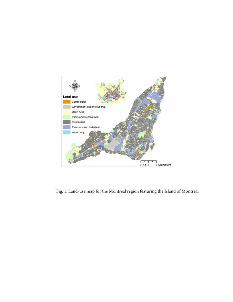
Fig. 1. Land-use map for the Montreal region featuring the Island of Montreal

Fig. 2. Visualizing NO2 levels across the Montreal region. Average NO2 concentrations are illustrated at five different levels with green shades representing the lowest concentrations and red shades the highest concentrations.

(a) (b)

Fig. 3. Map of land-use clusters including: Cluster 1 characterized by TAZs with higher population density, higher governmental and institutional areas, denser road network and better access to metro and bus service; Cluster 2 characterized by TAZs with higher industrial density and lower residential, governmental, and institutional densities and poorer transit accessibility; Cluster 3 characterized by TAZs with higher residential density and lower industrial density; and Cluster 4 characterized by TAZs with fewer points of interest, lower population density and lower accessibility to transit service. The home locations of individuals in the OD survey are presented in Fig 3b.

Fig. 4. Descriptive statistics for individual NOx emissions (all drivers)

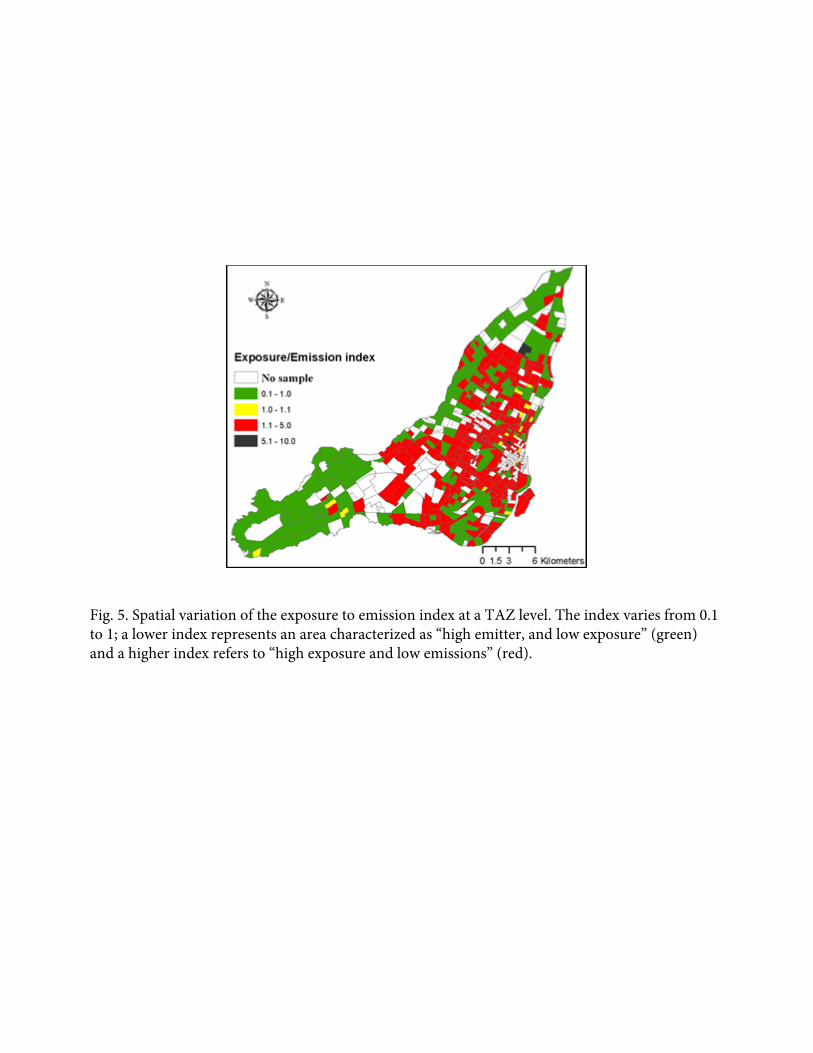
Fig. 5. Spatial variation of the exposure to emission index at a TAZ level. The index varies from 0.1 to 1; a lower index represents an area characterized as “high emitter, and low exposure” (green) and a higher index refers to “high exposure and low emissions” (red).

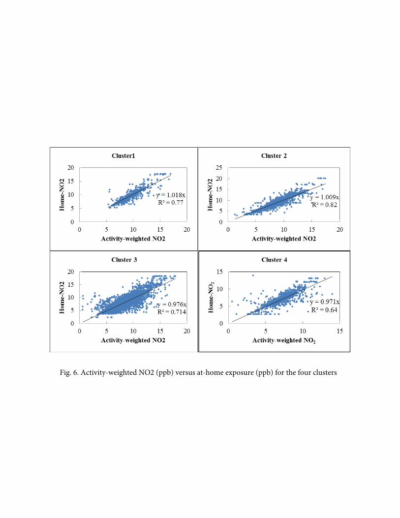
Fig. 6. Activity-weighted NO2 (ppb) versus at-home exposure (ppb) for the four clusters

Cluster 1 Cluster 2

Cluster 3 Cluster 4

[0,Cmin) (Cmax,+ ∞) f1 22.47 13.48 f2 13.56 11.67

[0,Cmin)

f1 21.99 f2 17.80

[0,Cmin) (Cmax,+ ∞) f1 19.01 19.57 f2 14.25 22.80

[0,Cmin) (Cmax,+ ∞) f1 15.79 23.83 f2 17.75 21.10

(Cmax,+ ∞) 18.20 18.06

Fig. 7. Distribution of differences between activity-weighted exposures and at-home concentrations. f1 and f2 represent the percentages of drivers (f1) and of transit riders (f2) with differences between activity-weighted exposures and at-home concentrations that are higher or lower than the mean by 20%. Cmin represents the mean difference minus 20%; Cmax represents the mean difference plus 20%

Table 1. Results of factor analysis and cluster analysis

Factor Analysis Results

Components

Factors Public Transit

Road

Network Point of Interests

(Metro & Bus) (AMT Train)

Density of Bus Stops in TAZ 0.645 NA NA

Density of STM Metro Lines in TAZ 0.827 NA NA

Density of AMT Train Lines in TAZ 0.811 NA NA

Density of AMT Train Stations in TAZ 0.821 NA NA

Density of STM Metro Stations in TAZ 0.817 NA NA

Density of Major Roads in TAZ NA NA 0.936 NA

Density of Highways in TAZ NA NA 0.837 NA

Density of Minor Roads in TAZ NA NA 0.736 NA

Density of Restaurants in TAZ NA NA NA 0.947

Density of Bars in TAZ NA NA NA 0.669

Density of All other types of Commercials NA NA NA 0.883

Summary statistics

Eigen value 1.82 1.29 2.12 2.12

% of variance accounted by the component 36.41 25.85 70.50 70.80

Cluster Analysis Results: Cluster 1 Cluster 2 Cluster 3 Cluster 4

Mean SD Mean SD Mean SD Mean SD

Number of TAZs in Cluster 171 - 275 - 659 - 447 -

Population Density 23.18 19.61 8.52 6.80 8.82 5.94 2.17 2.97

Residential Density 0.39 0.29 0.24 0.26 0.71 0.15 0.17 0.16

Industrial Density 0.11 0.16 0.49 0.31 0.08 0.09 0.04 0.07

Governmental & Institutional Density 0.27 0.33 0.02 0.06 0.046 0.07 0.013 0.04

Average Income (1000$) 59.55 27.22 76.89 43.20 59.87 18.33 67.94 16.37

Point of Interests 1.14 2.66 -0.11 0.31 -0.08 0.31 -0.25 0.07

Road Network 1.16 1.69 0.25 0.90 0.12 0.61 -0.77 0.42

Transit (Metro-Bus) 1.36 2.40 -0.15 0.38 -0.01 0.43 -0.42 0.13

Transit (AMT Train) 0.46 2.73 0.15 0.78 -0.11 0.30 -0.11 0.12

Table 2. Linear regression of NOx emissions (R2 = 0.33)

Category Variable

t-stat

Constant 0.407 19.197

Gender Male 0.039 3.545

Female - -

Status

Employed-Part-time 0.060 2.081

Employed-Full-time 0.131 6.437

Student 0.212 6.325

Retired -0.046 -1.995

Other - -

Age

16-25

26-40

41-60 0.031 2.756

>60 - -

Vehicle Age

and Type

PC ≥ 2000 - -

PC < 2000 0.555 44.589

PT ≥ 2000 0.170 10.951

PT < 2000 0.740 35.834

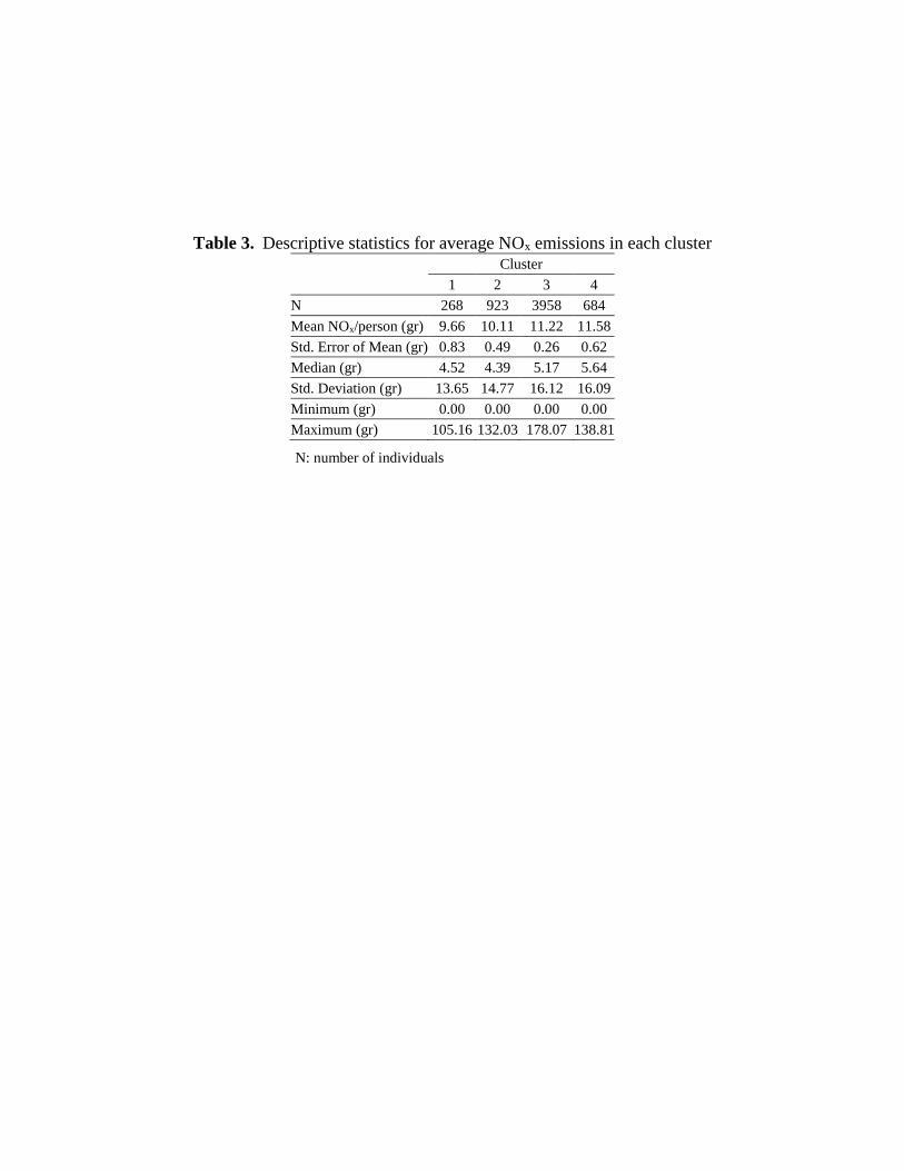
Table 3. Descriptive statistics for average NOx emissions in each cluster

Cluster

1 2 3 4

N 268 923 3958 684

Mean NOx/person (gr) 9.66 10.11 11.22 11.58

Std. Error of Mean (gr) 0.83 0.49 0.26 0.62

Median (gr) 4.52 4.39 5.17 5.64

Std. Deviation (gr) 13.65 14.77 16.12 16.09

Minimum (gr) 0.00 0.00 0.00 0.00

Maximum (gr) 105.16 132.03 178.07 138.81

N: number of individuals

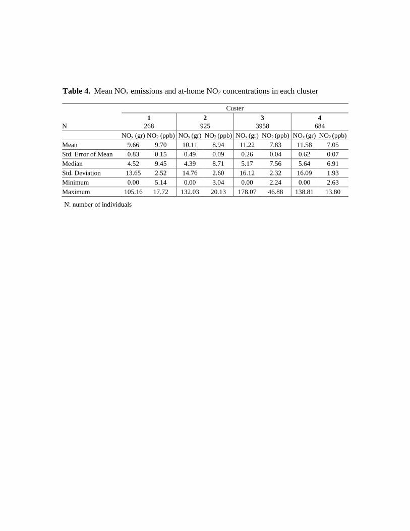
Table 4. Mean NOx emissions and at-home NO2 concentrations in each cluster

Custer

N

1

268

2

925

3

3958

4

684

NOx (gr) NO2 (ppb) NOx (gr) NO2 (ppb) NOx (gr) NO2 (ppb) NOx (gr) NO2 (ppb)

Mean 9.66 9.70 10.11 8.94 11.22 7.83 11.58 7.05

Std. Error of Mean 0.83 0.15 0.49 0.09 0.26 0.04 0.62 0.07

Median 4.52 9.45 4.39 8.71 5.17 7.56 5.64 6.91

Std. Deviation 13.65 2.52 14.76 2.60 16.12 2.32 16.09 1.93

Minimum 0.00 5.14 0.00 3.04 0.00 2.24 0.00 2.63

Maximum 105.16 17.72 132.03 20.13 178.07 46.88 138.81 13.80

N: number of individuals

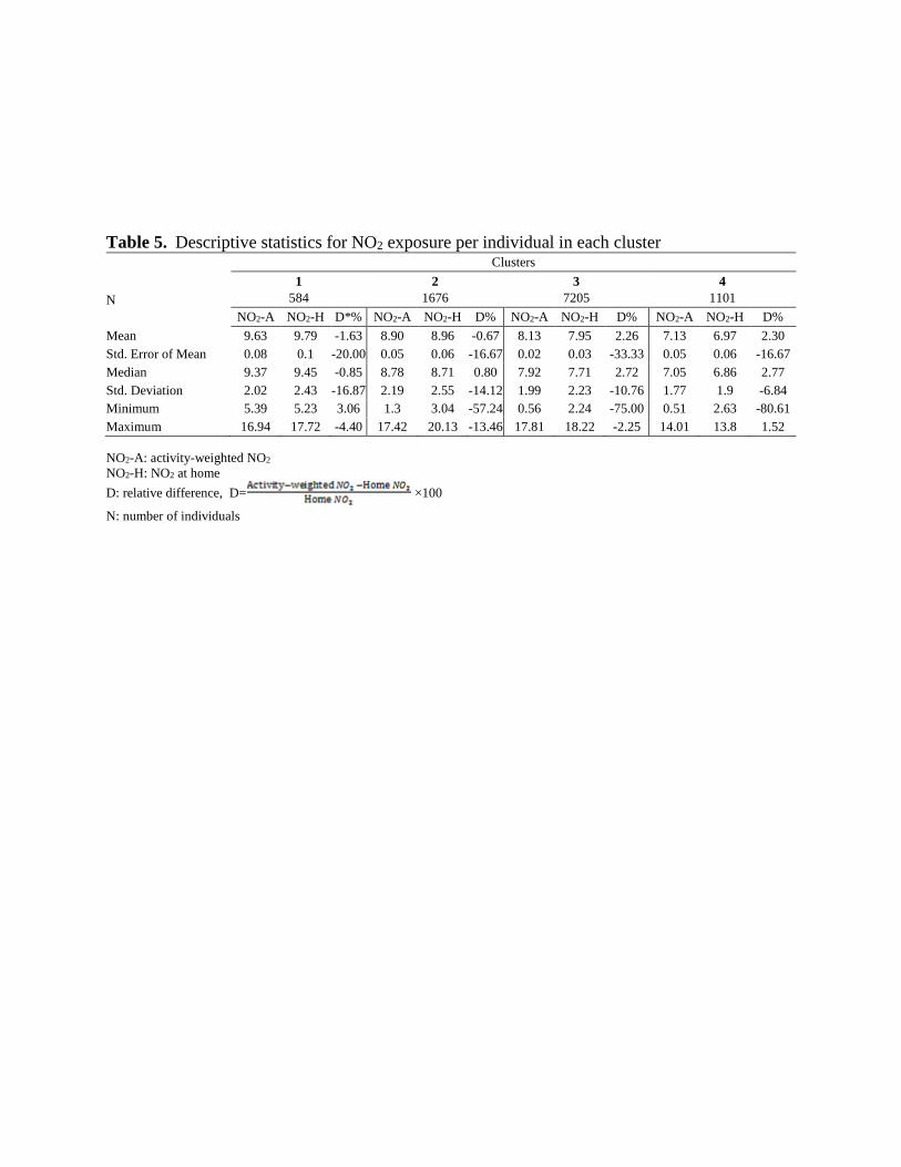
Table 5. Descriptive statistics for NO2 exposure per individual in each cluster

N

Clusters

1

584

2

1676

3

7205

4

1101

NO2-A NO2-H D*% NO2-A NO2-H D% NO2-A NO2-H D% NO2-A NO2-H D%

Mean 9.63 9.79 -1.63 8.90 8.96 -0.67 8.13 7.95 2.26 7.13 6.97 2.30

Std. Error of Mean 0.08 0.1 -20.00 0.05 0.06 -16.67 0.02 0.03 -33.33 0.05 0.06 -16.67

Median 9.37 9.45 -0.85 8.78 8.71 0.80 7.92 7.71 2.72 7.05 6.86 2.77

Std. Deviation 2.02 2.43 -16.87 2.19 2.55 -14.12 1.99 2.23 -10.76 1.77 1.9 -6.84

Minimum 5.39 5.23 3.06 1.3 3.04 -57.24 0.56 2.24 -75.00 0.51 2.63 -80.61

Maximum 16.94 17.72 -4.40 17.42 20.13 -13.46 17.81 18.22 -2.25 14.01 13.8 1.52

NO2-A: activity-weighted NO2

NO2-H: NO2 at home

D: relative difference, D= ×100

N: number of individuals