Proceedings of the 2nd International Workshop on Independent Component Analysis and Blind Signal Separation, 633-44, 2000.

INDEPENDENT COMPONENT ANALYSIS OF BIOMEDICAL SIGNALS*

Tzyy-Ping Jung (1,2), Scott Makeig (1,4), Te-Won Lee (1,2), Martin J. McKeown (5,6,7), Glen Brown (1), Anthony J. Bell (1), and Terrence J. Sejnowski (1,2,3)

(1) Computational Neurobiology Laboratory, Howard Hughes Medical Institute The Salk Institute for Biological

Studies; (2) Institute for Neural Computation, University of California San Diego, La Jolla CA; (3) Department of Biology, University of California San Diego, La Jolla CA. (4) Naval Health Research Center, San Diego CA;

(5) Department of Medicine (Neurology), Duke University (6) Brain Imaging and Analysis Center (BIAC), Duke University; (7) Center for Cognitive Neuroscience, Duke University, Durham, NC

{jung,scott,tewon,martin,glen,tony,terry}@salk.edu

*

A color version of this article can be downloaded from http://www.cnl.salk.edu/~jung/ica.html

ABSTRACT Biomedical signals from many sources including hearts, brains and endocrine systems pose a challenge to researchers who may have to separate weak signals arriving from multiple sources contaminated with artifacts and noise. The analysis of these signals is important both for research and for medical diagnosis and treatment. The applications of Independent Component Analysis (ICA) to biomedical signals is a rapidly expanding area of research and many groups are now actively engaged in exploring the potential of blind signal separation and signal deconvolution for revealing new information about the brain and body. In this review, we survey some recent applications of ICA to a variety of electrical, magnetic and hemodynamic measurements, drawing primarily from our own research.

1. INTRODUCTION

The goal of this review is to provide an overview of recent applications of ICA to biomedical signal processing, with a focus on recordings from the brain. Because it is often difficult to interpret neural recordings, we begin, in Section 2, with an analysis of the electrocardiogram (ECG) whose signals are better understood. This application also illustrates questions concerning the assumptions that are tacitly made in applying ICA to biological data. In Sections 3-6, we show how ICA can be applied to the electroencephalogram (EEG). Although these weak signals recorded from the surface of the scalp have been studied for near 100 years, their origins and relationship to brain function remains obscure. ICA may be helpful in identifying different types of generators of the EEG as well as its magnetic counterpart (MEG). Finally, we show in Section 7 that ICA can also be used to analyze hemodynamic signals from the brain recorded using functional magnetic resonance imaging (fMRI). This exciting new area of research allows neuroscientists to noninvasively measure brain activity in humans

indirectly through changes in blood flow. In all of these examples, great care must be taken to examine the validity of the assumptions that are used by ICA to derive a decomposition of the observed signals. Some new methods are summarized in Appendix. For biomedical time series analysis (EEG, ECG, etc), multiplying the input data matrix by the ‘unmixing’ matrix at the end of ICA training gives a new matrix whose rows, called the component activations, are the time courses of relative strengths or activity levels (and relative polarities) of the respective independent components. The columns of the inverse of the unmixing matrix give the relative projection strengths (and polarities) of the respective components onto each of the sensors. The projection of the ith independent component onto the original data channels is given by the outer product of the ith row of the component activation matrix with the ith column of the inverse unmixing matrix, and is in the original units (e.g. µV).

2. ELECTROCARDIOGRAMS (ECGs)

Several important issues in the application of ICA to biomedical data can be illustrated by the analysis of electrical signals from the heart. Signals recorded from the surface of the chest and abdomen arising from the beating heart are used by physicians to diagnose heart disease. Different parts of the heart such as the atria and ventricles produce different spatial and temporal patterns of electrical activity on the body surface. Recordings are typically made from multiple locations, each reflecting a different mixture of heart components. ECGs appear to satisfy some of the conditions for ICA: 1) Current from the different sources is mixed linearly at the ECG electrodes; 2) Time delays in signal transmission are negligible; 3) There appear to be fewer sources than mixtures; and 4) Sources have non-Gaussian voltage distributions. However, movements of the heart such as contraction of the chambers during beating violates the ICA assumption of spatial stationarity of the

634

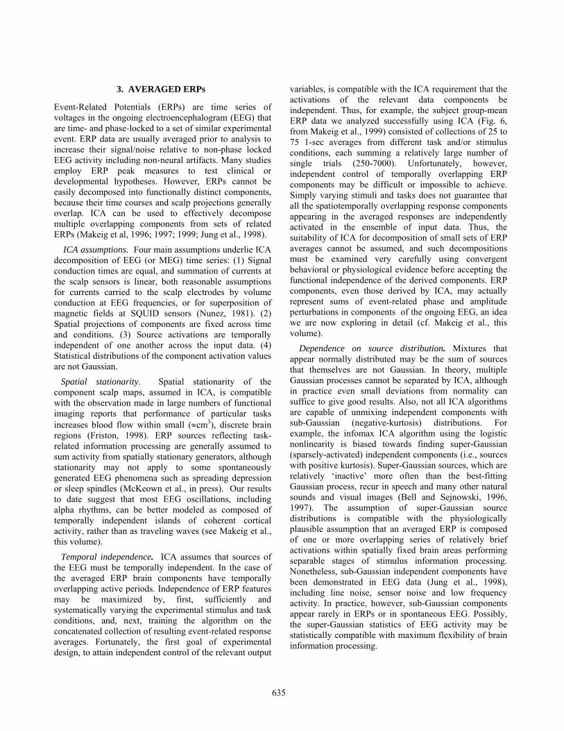
sources. The presence of moving waves of electrical activity across the heart also means that the activity of a single chamber may be taken for multiple sources by ICA. Another assumption of the ICA model, the independence between sources, has also lead to some confusion. For ICA, independence only refers to lack of dependency between coincident source activations, and not to possible time-delay dependencies. Artifacts, such as those introduced by small movements of the electrical contacts should be reasonably independent of signals originating from the heart. Signals generated by different parts of the heart during the cardiac cycle can also be separated by ICA if they are generated at different times or if there is jitter in the relative timing of overlapping signal sources. Here, we illustrate the ICA decomposition of maternal and fetal ECGs recorded simultaneously from cutaneous electrodes placed on the mother’s abdomen and chest (De Moor, 1997; Cardoso, 1998). Each ECG electrode was sampled for 12.5 seconds at 200 Hz (Figure 1A, left panel). In channels 1-5, measured from the abdominal region, the fetal ECG is barely visible. Channels 6-8 were recorded from the mother’s chest region; here the fetal signals are not visible. These ECG data were treated as observed mixtures of independent ECG sources. Figure 1A (right panel) shows the eight independent components derived by the extended infomax ICA algorithm (Lee et al., 1999a). Components 1-4 evidently account for maternal ECG

with a beat rate of ~72, whereas components 6 and 8 account for the fetal ECG beating at ~106/min. The sources of Components 5 and 7 are unknown. To examine the dynamics of each component, we first aligned the data to peaks in the mother’s heartbeats, then averaged the data and overlaid the projections of components 1-4 onto the averaged ECG at electrode 8 (Figure 1B, left panel). It is thought that the P wave in the ECG corresponds to the depolarization of the atria, and the QRS complex to the repolarization of atria overlapped with the depolarization of the ventricles. ICA decomposed the maternal ECG into four components presumably accounting for distinct but overlapping periods of activation of atria and ventricles. The decomposition might potentially be useful to separate the depolarization/repolarization of the ventricles and atria. However, further experiments will be necessary to interpret the ICA decomposition physiologically. Figure 1B (right panel) shows the averaged peak-aligned fetal ECG at electrode 2 plus the projections of components 6 and 8. Since the averaged fetal ECG has a very poor signal-to-noise ratio relative to dominant maternal ECG, averaging failed to eliminate vestiges of the large maternal ECG signals. The projections of components 6 and 8, however, show no sign of this interference, indicating that their activity accounted mainly for the fetal ECG. The ability of ICA to separate small vital signals from dominant cardiac signals may have future applications in the diagnosis of heart disease.

Figure 1: Decomposition of ECG using ICA (see also Cardoso, 1998). (A) (Left panel) A 3-sec portion of ECG time series containing prominent maternal ECG. (Right panel) Eight corresponding ICA components whose activations account for maternal ECG (1-4), fetal ECG (6 and 8) and noise (5 and 7), respectively. (B) (Left panel) The data were aligned to the peaks of the maternal heartbeats and averaged to form an averaged maternal ECG. The signal (faint trace) at one of the chest channels (channel 8) is shown. (Right panel) The same data aligned to the fetal ECG peaks and overlaid at one of the abdominal sites (channel 2), plus the projections of components 6 and 8. Data from Database for the Identification of Systems (De Moor, 1997).

B

A

P

Q

R

S

635

3. AVERAGED ERPs

Event-Related Potentials (ERPs) are time series of voltages in the ongoing electroencephalogram (EEG) that are time- and phase-locked to a set of similar experimental event. ERP data are usually averaged prior to analysis to increase their signal/noise relative to non-phase locked EEG activity including non-neural artifacts. Many studies employ ERP peak measures to test clinical or developmental hypotheses. However, ERPs cannot be easily decomposed into functionally distinct components, because their time courses and scalp projections generally overlap. ICA can be used to effectively decompose multiple overlapping components from sets of related ERPs (Makeig et al, 1996; 1997; 1999; Jung et al., 1998).

ICA assumptions. Four main assumptions underlie ICA decomposition of EEG (or MEG) time series: (1) Signal conduction times are equal, and summation of currents at the scalp sensors is linear, both reasonable assumptions for currents carried to the scalp electrodes by volume conduction at EEG frequencies, or for superposition of magnetic fields at SQUID sensors (Nunez, 1981). (2) Spatial projections of components are fixed across time and conditions. (3) Source activations are temporally independent of one another across the input data. (4) Statistical distributions of the component activation values are not Gaussian.

Spatial stationarity. Spatial stationarity of the component scalp maps, assumed in ICA, is compatible with the observation made in large numbers of functional imaging reports that performance of particular tasks increases blood flow within small (≈cm3), discrete brain regions (Friston, 1998). ERP sources reflecting task-related information processing are generally assumed to sum activity from spatially stationary generators, although stationarity may not apply to some spontaneously generated EEG phenomena such as spreading depression or sleep spindles (McKeown et al., in press). Our results to date suggest that most EEG oscillations, including alpha rhythms, can be better modeled as composed of temporally independent islands of coherent cortical activity, rather than as traveling waves (see Makeig et al., this volume).

Temporal independence. ICA assumes that sources of the EEG must be temporally independent. In the case of the averaged ERP brain components have temporally overlapping active periods. Independence of ERP features may be maximized by, first, sufficiently and systematically varying the experimental stimulus and task conditions, and, next, training the algorithm on the concatenated collection of resulting event-related response averages. Fortunately, the first goal of experimental design, to attain independent control of the relevant output

variables, is compatible with the ICA requirement that the activations of the relevant data components be independent. Thus, for example, the subject group-mean ERP data we analyzed successfully using ICA (Fig. 6, from Makeig et al., 1999) consisted of collections of 25 to 75 1-sec averages from different task and/or stimulus conditions, each summing a relatively large number of single trials (250-7000). Unfortunately, however, independent control of temporally overlapping ERP components may be difficult or impossible to achieve. Simply varying stimuli and tasks does not guarantee that all the spatiotemporally overlapping response components appearing in the averaged responses are independently activated in the ensemble of input data. Thus, the suitability of ICA for decomposition of small sets of ERP averages cannot be assumed, and such decompositions must be examined very carefully using convergent behavioral or physiological evidence before accepting the functional independence of the derived components. ERP components, even those derived by ICA, may actually represent sums of event-related phase and amplitude perturbations in components of the ongoing EEG, an idea we are now exploring in detail (cf. Makeig et al., this volume).

Dependence on source distribution. Mixtures that appear normally distributed may be the sum of sources that themselves are not Gaussian. In theory, multiple Gaussian processes cannot be separated by ICA, although in practice even small deviations from normality can suffice to give good results. Also, not all ICA algorithms are capable of unmixing independent components with sub-Gaussian (negative-kurtosis) distributions. For example, the infomax ICA algorithm using the logistic nonlinearity is biased towards finding super-Gaussian (sparsely-activated) independent components (i.e., sources with positive kurtosis). Super-Gaussian sources, which are relatively ‘inactive’ more often than the best-fitting Gaussian process, recur in speech and many other natural sounds and visual images (Bell and Sejnowski, 1996, 1997). The assumption of super-Gaussian source distributions is compatible with the physiologically plausible assumption that an averaged ERP is composed of one or more overlapping series of relatively brief activations within spatially fixed brain areas performing separable stages of stimulus information processing. Nonetheless, sub-Gaussian independent components have been demonstrated in EEG data (Jung et al., 1998), including line noise, sensor noise and low frequency activity. In practice, however, sub-Gaussian components appear rarely in ERPs or in spontaneous EEG. Possibly, the super-Gaussian statistics of EEG activity may be statistically compatible with maximum flexibility of brain information processing.

636

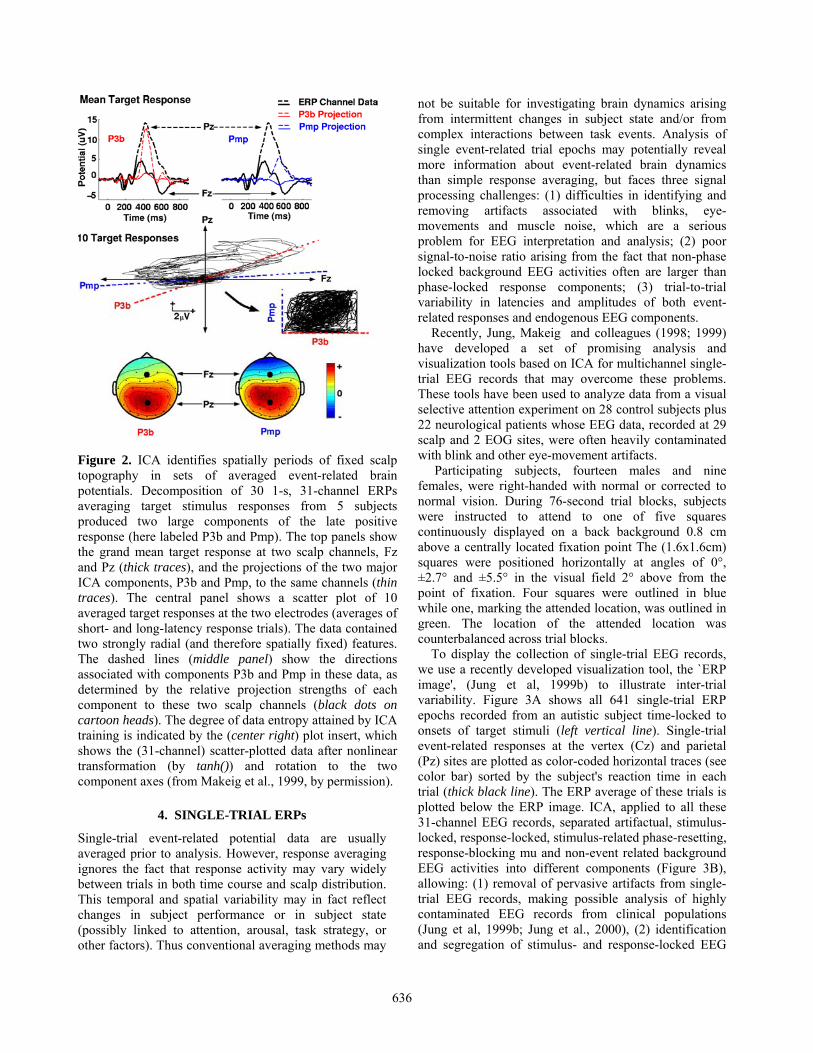
Figure 2. ICA identifies spatially periods of fixed scalp topography in sets of averaged event-related brain potentials. Decomposition of 30 1-s, 31-channel ERPs averaging target stimulus responses from 5 subjects produced two large components of the late positive response (here labeled P3b and Pmp). The top panels show the grand mean target response at two scalp channels, Fz and Pz (thick traces), and the projections of the two major ICA components, P3b and Pmp, to the same channels (thin traces). The central panel shows a scatter plot of 10 averaged target responses at the two electrodes (averages of short- and long-latency response trials). The data contained two strongly radial (and therefore spatially fixed) features. The dashed lines (middle panel) show the directions associated with components P3b and Pmp in these data, as determined by the relative projection strengths of each component to these two scalp channels (black dots on cartoon heads). The degree of data entropy attained by ICA training is indicated by the (center right) plot insert, which shows the (31-channel) scatter-plotted data after nonlinear transformation (by tanh()) and rotation to the two component axes (from Makeig et al., 1999, by permission).

4. SINGLE-TRIAL ERPs

Single-trial event-related potential data are usually averaged prior to analysis. However, response averaging ignores the fact that response activity may vary widely between trials in both time course and scalp distribution. This temporal and spatial variability may in fact reflect changes in subject performance or in subject state (possibly linked to attention, arousal, task strategy, or other factors). Thus conventional averaging methods may

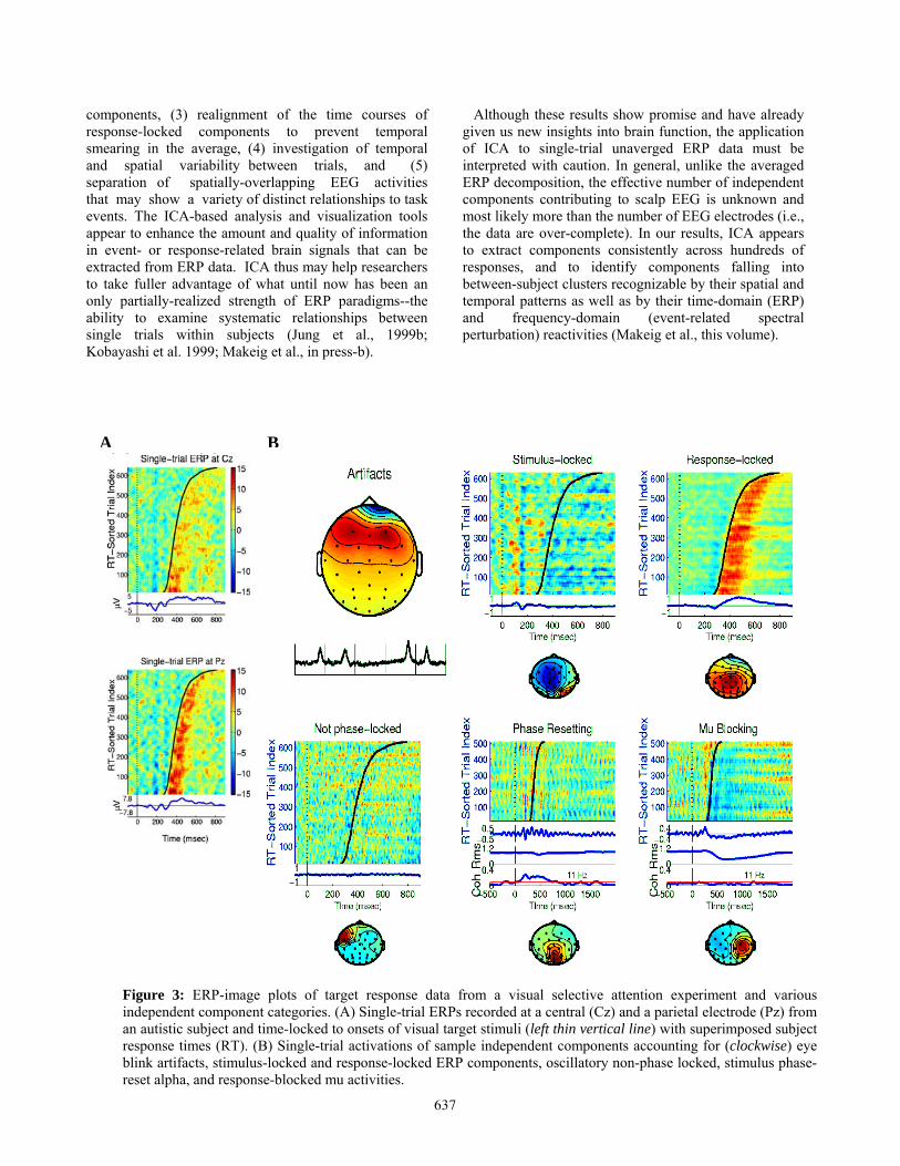
not be suitable for investigating brain dynamics arising from intermittent changes in subject state and/or from complex interactions between task events. Analysis of single event-related trial epochs may potentially reveal more information about event-related brain dynamics than simple response averaging, but faces three signal processing challenges: (1) difficulties in identifying and removing artifacts associated with blinks, eye-movements and muscle noise, which are a serious problem for EEG interpretation and analysis; (2) poor signal-to-noise ratio arising from the fact that non-phase locked background EEG activities often are larger than phase-locked response components; (3) trial-to-trial variability in latencies and amplitudes of both event-related responses and endogenous EEG components. Recently, Jung, Makeig and colleagues (1998; 1999) have developed a set of promising analysis and visualization tools based on ICA for multichannel single-trial EEG records that may overcome these problems. These tools have been used to analyze data from a visual selective attention experiment on 28 control subjects plus 22 neurological patients whose EEG data, recorded at 29 scalp and 2 EOG sites, were often heavily contaminated with blink and other eye-movement artifacts. Participating subjects, fourteen males and nine females, were right-handed with normal or corrected to normal vision. During 76-second trial blocks, subjects were instructed to attend to one of five squares continuously displayed on a back background 0.8 cm above a centrally located fixation point The (1.6x1.6cm) squares were positioned horizontally at angles of 0°, ±2.7° and ±5.5° in the visual field 2° above from the point of fixation. Four squares were outlined in blue while one, marking the attended location, was outlined in green. The location of the attended location was counterbalanced across trial blocks. To display the collection of single-trial EEG records, we use a recently developed visualization tool, the `ERP image', (Jung et al, 1999b) to illustrate inter-trial variability. Figure 3A shows all 641 single-trial ERP epochs recorded from an autistic subject time-locked to onsets of target stimuli (left vertical line). Single-trial event-related responses at the vertex (Cz) and parietal (Pz) sites are plotted as color-coded horizontal traces (see color bar) sorted by the subject's reaction time in each trial (thick black line). The ERP average of these trials is plotted below the ERP image. ICA, applied to all these 31-channel EEG records, separated artifactual, stimulus-locked, response-locked, stimulus-related phase-resetting, response-blocking mu and non-event related background EEG activities into different components (Figure 3B), allowing: (1) removal of pervasive artifacts from single-trial EEG records, making possible analysis of highly contaminated EEG records from clinical populations (Jung et al, 1999b; Jung et al., 2000), (2) identification and segregation of stimulus- and response-locked EEG

637

components, (3) realignment of the time courses of response-locked components to prevent temporal smearing in the average, (4) investigation of temporal and spatial variability between trials, and (5) separation of spatially-overlapping EEG activities that may show a variety of distinct relationships to task events. The ICA-based analysis and visualization tools appear to enhance the amount and quality of information in event- or response-related brain signals that can be extracted from ERP data. ICA thus may help researchers to take fuller advantage of what until now has been an only partially-realized strength of ERP paradigms--the ability to examine systematic relationships between single trials within subjects (Jung et al., 1999b; Kobayashi et al. 1999; Makeig et al., in press-b).

Although these results show promise and have already given us new insights into brain function, the application of ICA to single-trial unaverged ERP data must be interpreted with caution. In general, unlike the averaged ERP decomposition, the effective number of independent components contributing to scalp EEG is unknown and most likely more than the number of EEG electrodes (i.e., the data are over-complete). In our results, ICA appears to extract components consistently across hundreds of responses, and to identify components falling into between-subject clusters recognizable by their spatial and temporal patterns as well as by their time-domain (ERP) and frequency-domain (event-related spectral perturbation) reactivities (Makeig et al., this volume).

Figure 3: ERP-image plots of target response data from a visual selective attention experiment and various independent component categories. (A) Single-trial ERPs recorded at a central (Cz) and a parietal electrode (Pz) from an autistic subject and time-locked to onsets of visual target stimuli (left thin vertical line) with superimposed subject response times (RT). (B) Single-trial activations of sample independent components accounting for (clockwise) eye blink artifacts, stimulus-locked and response-locked ERP components, oscillatory non-phase locked, stimulus phase-reset alpha, and response-blocked mu activities.

(A) (B)

A B

638

5. EVENT-RELATED ‘ALPHA RINGING’

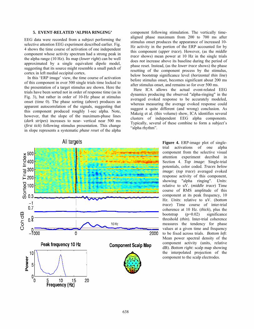
EEG data were recorded from a subject performing the selective attention EEG experiment described earlier. Fig. 4 shows the time course of activation of one independent component whose activity spectrum had a strong peak in the alpha range (10 Hz). Its map (lower right) can be well approximated by a single equivalent dipole model, suggesting that its source might resemble a small patch of cortex in left medial occipital cortex. In this ‘ERP image’ view, the time course of activation of this component in over 500 single trials time locked to the presentation of a target stimulus are shown. Here the trials have been sorted not in order of response time (as in Fig. 3), but rather in order of 10-Hz phase at stimulus onset (time 0). The phase sorting (above) produces an apparent autocorrelation of the signals, suggesting that this component produced roughly 1-sec alpha. Note, however, that the slope of the maximum-phase lines (dark stripes) increases to near- vertical near 500 ms (first tick) following stimulus presentation. This change in slope represents a systematic phase reset of the alpha

component following stimulation. The vertically time-aligned phase maximum from 200 to 700 ms after stimulus onset produces the appearance of increased 10-Hz activity in the portion of the ERP accounted for by this component (upper trace). However, (as the middle trace shows) mean power at 10 Hz in the single trials does not increase above its baseline during the period of phase reset. Instead, (as the lower trace shows) the phase resetting of the component process by the stimulus, below bootstrap significance level (horizontal thin line) before stimulus onset, becomes significant about 200 ms after stimulus onset, and remains so for over 500 ms. Here ICA allows the actual event-related EEG dynamics producing the observed "alpha-ringing" in the averaged evoked response to be accurately modeled, whereas measuring the average evoked response could suggest a quite different (and wrong) conclusion. As Makeig et al. (this volume) show, ICA identifies several clusters of independent EEG alpha components. Typically, several of these combine to form a subject’s “alpha rhythm”.

Figure 4. ERP-image plot of single-trial activations of one alpha component from the selective visual attention experiment decribed in Section 4. Top image: Single-trial potentials, color coded. Traces below image: (top trace) averaged evoked response activity of this component, showing "alpha ringing". Units: relative to uV. (middle trace) Time course of RMS amplitude of this component at its peak frequency, 10 Hz. Units: relative to uV. (bottom trace) Time course of inter-trial coherence at 10 Hz. (thick), plus the bootstrap (p=0.02) significance threshold (thin). Inter-trial coherence measures the tendency for phase values at a given time and frequency to be fixed across trials. Bottom left: Mean power spectral density of the component activity (units, relative dB). Bottom right: scalp map showing the interpolated projection of the component to the scalp electrodes.

639

6. ALERTNESS MONITORING USING AN ICA MIXTURE MODEL

EEG and behavioral data were collected to develop a method of objectively monitoring the alertness of operators listening for weak signals in background noise (Makeig & Inlow, 1993; Jung et al., 1997). Subjects were instructed to keep their eyes closed and to push a button whenever they detected an above-threshold auditory target stimulus. Auditory targets were 350-ms increases in the intensity of a 62-dB white noise background, 6 dB above their threshold of detectability, presented at random time intervals at a mean rate of 10/min, and superimposed on a continuous 39-Hz click train evoking a 39-Hz steady-state response. Short, and task-irrelevant probe tones of two frequencies (568 and 1098 Hz) were interspersed between the target noise bursts at 2-4 s intervals. EEG was collected from thirteen electrodes located at sites of the International 10-20 System, referred to the right mastoid, at a sampling rate of 312.5 Hz. A bipolar diagonal electrooculogram (EOG) channel was also recorded. Hits were defined as targets responded to within a 100-3000 ms post-stimulus window. Lapses were targets not responded to (because of drowsiness or loss of vigilance). A continuous performance measure, local error rate, was computed by convolving the irregularly-sampled performance index time series (Hit=0/Lapse=1) with a 95-sec smoothing window advanced through the data in 1.64 sec steps.

The ICA mixture model can be used for unsupervised classification and tracking non-stationary signals (Lee et al., 1999c, see Appendix). When this model was applied to the 14-channel, 28-min EEG data, the model segregated the data into different states or classes. This automatic switching allowed the model to model the spatial independent component structure in each class.

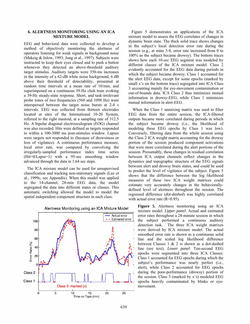
Figure 5 demonstrates an applications of the ICA mixture model to assess the EEG correlates of changes in dynamic brain state. The thick solid trace shows changes in the subject’s local detection error rate during the session (e.g., at mins 3-8, error rate increased from 0 to 100% as the subject became drowsy). The bottom traces shows how each 10-sec EEG segment was modeled by different classes of the ICA mixture model. Class 2 evidently accounted for the EEG data during periods in which the subject became drowsy. Class 1 accounted for the alert EEG data, except for some epochs (marked by small x’s on the bottom trace) segregated into ICA Class 3 accounting mainly for eye-movement contamination or out-of-bounds data. ICA Class 2 thus minimizes mutual information in drowsy-EEG, while Class 1 minimizes mutual information in alert-EEG.

When the Class 1 unmixing matrix was used to filter EEG data from the entire session, the ICA-filtered outputs became more correlated during periods in which the subject became drowsy (i.e., the likelihood of modeling these EEG epochs by Class 1 was low). Conversely, filtering data from the whole session using the Class 2 ICA weight matrix accounting for the drowsy portion of the session produced component activations that were more correlated during the alert portions of the session. Presumably, these changes in residual correlation between ICA output channels reflect changes in the dynamics and topographic structure of the EEG signals between alert and drowsy brain states, and could be used to predict the level of vigilance of the subject. Figure 5 shows that the difference between the log likelihood measures of these two ICA weight matrices could estimate very accurately changes in the behaviorally-defined level of alertness throughout the session. The regressed difference (dot-dashed) was highly correlated with actual error rate (R=0.95).

Figure 5. Alertness monitoring using an ICA mixture model. Upper panel: Actual and estimated error rates throughout a 28-minute session in which the subject performed a continuous auditory detection task. The three ICA weight matrixes were derived by ICA mixture model. The actual smoothed error rate is shown as a continuous solid line and the scaled log likelihood difference between Classes 1 & 2 is shown as a dot-dashed line (see text). Lower panel: Ten-second EEG epochs were segmented into three ICA Classes: Class 1 accounted for EEG epochs during which the subject’s performance was nearly perfect (i.e., alert), while Class 2 accounted for EEG epochs during the poor-performance (drowsy) portion of the session. Class 3 (marked by x’s) modeled EEG epochs heavily contaminated by blinks or eye-movement.

640

7. FUNCTIONAL MAGNETIC RESONANCE IMAGING (fMRI)

The analysis of fMRI brain data is a challenging enterprise, as the fMRI signals have varied, unpredictable time courses that represent the summation of signals from hemodynamic changes as a result of neural activity, from motion and machine artifacts, and from physiological cardiac and respiratory pulsations, as well as possibly other signals. The relative contribution and exact form of each of these components is largely unknown, suggesting a role for blind separation methods, if the data can be placed in a form consistent with these models (McKeown, Jung et al. 1998; McKeown, Makeig et al. 1998; McKeown and Sejnowski 1998; McKeown 2000). The assumptions of ICA apply to fMRI data in a different way than to other time series analysis. Here the principal of brain modularity suggests that, as different brain regions perform distinct functions, these time courses of activity should be separable (though not necessarily independent). This, plus the relatively high 3-D spatial resolution of fMRI, allows ICA to identify spatially independent regions with distinguishable time courses. However, the principle of spatial independence of active brain areas is not absolute, and therefore the functional significance of independent fMRI components must also be validated by convergent physiological or behavioral evidence.

General Linear Model (GLM). Traditional methods of fMRI analysis (Friston 1996) are based on variants of the General Linear Model, i.e., X = Gβ + ε (1)

Where X is an n by v row mean-zero data matrix with n being the number of time points in the experiment and v being the total number of voxels in all slices, G is a specified n by p design matrix containing the time courses of all p factors hypothesized to modulate the BOLD signal, including the behavioral manipulations of the fMRI experiment, β is a p by v matrix of parameters to be estimated, and ε is a matrix of noise or residual errors typically assumed to be independent, zero-mean and Gaussian distributed, i.e. N(0,σ2). Once G is specified, standard regression techniques can be used to provide a least squares estimate for the parameters in β. The statistical significance of these parameters can be considered to constitute spatial maps (Friston 1996), one for each row in β, which correspond to the time courses specified in the columns of the design matrix. GLM assumes: (1) the design matrix is known without error, (2) time courses are white; (3) the β's follow a Gaussian distribution; and (4) the residuals are well-modeled by Gaussian noise.

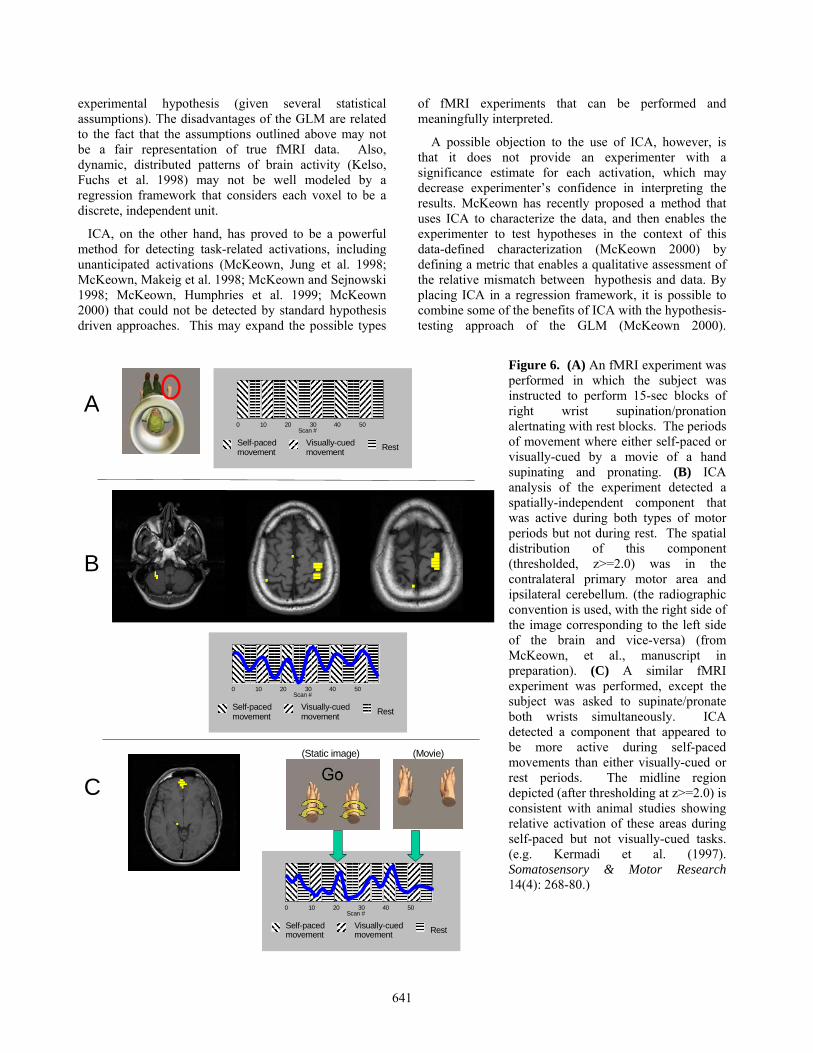
ICA Applied to fMRI Data. Using ICA, we can calculate an unmixing matrix, W, to calculate spatially independent components, C = WX, (2) where again, X is the n by v row mean-zero data matrix with n being the number of time points in the experiment and v being the total number of voxels, W is an n by n unmixing matrix, and C is an n by v matrix of n spatially independent components (sICs). If W is invertible, we may write, X = W-1C (3) An attractive interpretation of eqn (3) is that the columns of W-1 represent basis waveforms that can used to construct the observed voxel time courses described in the columns of X. These basis waveforms can be considered fundamental, as the projection on one basis waveform is independent of the projection on another (i.e., the rows of C are maximally independent). The similarity between ICA and the GLM can be seen by comparing eqns (1) and (3). Starting with equation (3) and performing the initial simple notation substitutions, W-1 → G and C → β, we have X = Gβ (4) which is equivalent to eqn (1) without the Gaussian error term. Note however the important teleological differences between equations (1) and (4): when regression equation is used (eqn 1), the design matrix G is specified by the examiner, while in eqn. (4) the matrix G is calculated from the data by the ICA algorithm, also determines β eqn. 2. That is, ICA does not reply on a priori knowledge about the time courses of brain activation and noise sources, and make only weak assumptions about their probability distributions. A Case Study. Figure 6 shows the results of applying ICA to a fMRI data set. The fMRI data were acquired when a subject performed 15-sec blocks of visually-cued or self-paced right wrist supination/pronation alternating with 15-sec rest blocks. ICA detected a spatially-independent component that was active during either types of motor activity but not during rest (Figure 6B). Figure 6C shows a similar fMRI experiment in which the subject was asked to supinate/pronate both wrists simultaneously. Here ICA detected a component more active during self-paced movements than either visually-cued or rest periods. Its midline, frontal polar location (depicted) is consistent with animal studies showing relative activation in this area during self-paced but not during visually-cued tasks.

Future Direction. In many respects, use of GLM and ICA are complimentary (Friston, 1998; McKeown & Sejnowski, 1998). The advantage of the GLM is that it allows the experimenter to check the statistical significance of activation corresponding to the

641

experimental hypothesis (given several statistical assumptions). The disadvantages of the GLM are related to the fact that the assumptions outlined above may not be a fair representation of true fMRI data. Also, dynamic, distributed patterns of brain activity (Kelso, Fuchs et al. 1998) may not be well modeled by a regression framework that considers each voxel to be a discrete, independent unit.

ICA, on the other hand, has proved to be a powerful method for detecting task-related activations, including unanticipated activations (McKeown, Jung et al. 1998; McKeown, Makeig et al. 1998; McKeown and Sejnowski 1998; McKeown, Humphries et al. 1999; McKeown 2000) that could not be detected by standard hypothesis driven approaches. This may expand the possible types

of fMRI experiments that can be performed and meaningfully interpreted.

A possible objection to the use of ICA, however, is that it does not provide an experimenter with a significance estimate for each activation, which may decrease experimenter’s confidence in interpreting the results. McKeown has recently proposed a method that uses ICA to characterize the data, and then enables the experimenter to test hypotheses in the context of this data-defined characterization (McKeown 2000) by defining a metric that enables a qualitative assessment of the relative mismatch between hypothesis and data. By placing ICA in a regression framework, it is possible to combine some of the benefits of ICA with the hypothesis- testing approach of the GLM (McKeown 2000).

Figure 6. (A) An fMRI experiment was performed in which the subject was instructed to perform 15-sec blocks of right wrist supination/pronation alertnating with rest blocks. The periods of movement where either self-paced or visually-cued by a movie of a hand supinating and pronating. (B) ICA analysis of the experiment detected a spatially-independent component that was active during both types of motor periods but not during rest. The spatial distribution of this component (thresholded, z>=2.0) was in the contralateral primary motor area and ipsilateral cerebellum. (the radiographic convention is used, with the right side of the image corresponding to the left side of the brain and vice-versa) (from McKeown, et al., manuscript in preparation). (C) A similar fMRI experiment was performed, except the subject was asked to supinate/pronate both wrists simultaneously. ICA detected a component that appeared to be more active during self-paced movements than either visually-cued or rest periods. The midline region depicted (after thresholding at z>=2.0) is consistent with animal studies showing relative activation of these areas during self-paced but not visually-cued tasks. (e.g. Kermadi et al. (1997). Somatosensory & Motor Research 14(4): 268-80.)

A

B

C

0 10 20 30 40 50Scan #

Self-pacedmovement

Visually-cuedmovement Rest

0 10 20 30 40 50Scan #

Self-pacedmovement

Visually-cuedmovement Rest

0 10 20 30 40 50Scan #

Self-pacedmovement

Visually-cuedmovement Rest

(Static image) (Movie)

642

8. DISCUSSION

Biomedical signals are a rich source of information about physiological processes, but they are often contaminated with artifacts and noise and are typically mixed in unknown combinations at every available sensor. As we have attempted to show here, ICA holds great promise for blindly separating artifacts from relevant signals and for further decomposing the mixed signals into subcomponents that may index the activity of functionally distinct generators. In addition to the analysis of EEG signals, ICA has also been applied to magnetoencephalographic (MEG) recordings (Vigario and Oja 1999), which carry signals from brain sources and are in part complementary to EEG signals. ICA has also been used to analyze data from Positron Emission Tomography (PET), a method for following changes in blood flow in the brain on slower time scales following the injection of radioactive isotopes into the bloodstream (Petersen et al., 2000). Other interesting applications of ICA are to the electrocorticogram (EcoG), direct measurements of electrical activity from the surface of the cortex (Makeig et al., in press-a), and to optical recordings of electrical activity from the surface of the cortex using voltage-sensitive dyes (Schoener et al., 1999). First clinical research applications of ICA include the analysis of EEG recordings during epileptic seizures (McKeown et al, in press-a). Although these results show promise and have already given us new insights into brain function, the application of ICA to biomedical signals is still in its infancy. Its results must always be validated using other more direct or convergent measures before we can have confidence in their interpretation. Toward this goal, we have analyzed simulated EEG recordings generated from a head model and dipole sources that include intrinsic noise and sensor noise (Makeig et al. in press a). This has given us some understanding of the conditions when ICA will fail to separate correlated sources of EEG signals. Another approach to validating ICA is to record simultaneously several types of signals, such as EEG and fMRI recordings, which should provide good spatial resolution (fMRI) and temporal resolution (EEG) (Jung, et al. 1999a). In sum, ICA has proven to be a valuable new analytic tool that will doubtless be applied fruitfully to many types of biomedical data.

9. APPENDIX: ICA MIXTURE MODEL

The extended version (Lee et al, 1999a) of the infomax ICA algorithm (Bell and Sejnowski, 1995) was used for all of the examples of biomedical signal processing summarized here. Comparisons with other methods can be found in the original papers where these results first

appeared. A Matlab ICA toolbox can be downloaded from http://www.cnl.salk.edu/~scott/ica.html.

In a mixture model (Duda & Hart, 1973), the observed data can be categorized into several mutually exclusive classes. When the data in each class are modeled as multivariate Gaussian, it is called a Gaussian mixture model. We generalize this by assuming the data in each class are generated by a linear combination of independent, non-Gaussian sources as assumed by ICA. We call this model an ICA mixture model. This allows modeling of classes with non-Gaussian structure, e.g., platykurtic or leptokurtic probability density functions. The algorithm for learning the parameters of the model uses gradient ascent to maximize the log likelihood function. In previous applications this approach showed improved performance in data classification problems (Lee et al., 1999a), performed blind signal separation in non-stationary environments (Lee et al., 2000), and learned efficient codes for representing different types of images (Lee et al. 1999b). Assume that the data are drawn independently and generated by a mixture density model (Duda & Hart, 1973). The likelihood of the data is given by the joint density: The mixture density is where Θ are the unknown parameters for each component densities. C denotes the class and it is assumed that the number of classes K, are known in advance. Assume that the component densities are non-Gaussian and the data within each class are described by:

where A is a N x M scalar matrix and b is the bias vector. The A matrix is called the mixing matrix in standard ICA. However, we refer to A as the basis matrix to distinguish this from the word mixture in the mixture model. The vector s is called the source vector and these are also the coefficients for each basis function. It is assumed that the individual sources within each class are mutually independent across a data ensemble. For simplicity, we consider the case where the number of sources is equal to the number of mixtures. Figure A.1 shows a simple example of a dataset describable by an ICA mixture model. Each class was generated using a different A and b. Class ‘o’ was generated by two uniformly distributed sources,

},,,{ 21 TxxxX K=∏=

Θ=ΘT

ttpp

1

)|()|( xX

ktkt bsAx +=

∑=

=ΘK

kkkktt CpCpp

1

)(),|()|( θxx },,,{ 21 Kθθθ K=Θ

643

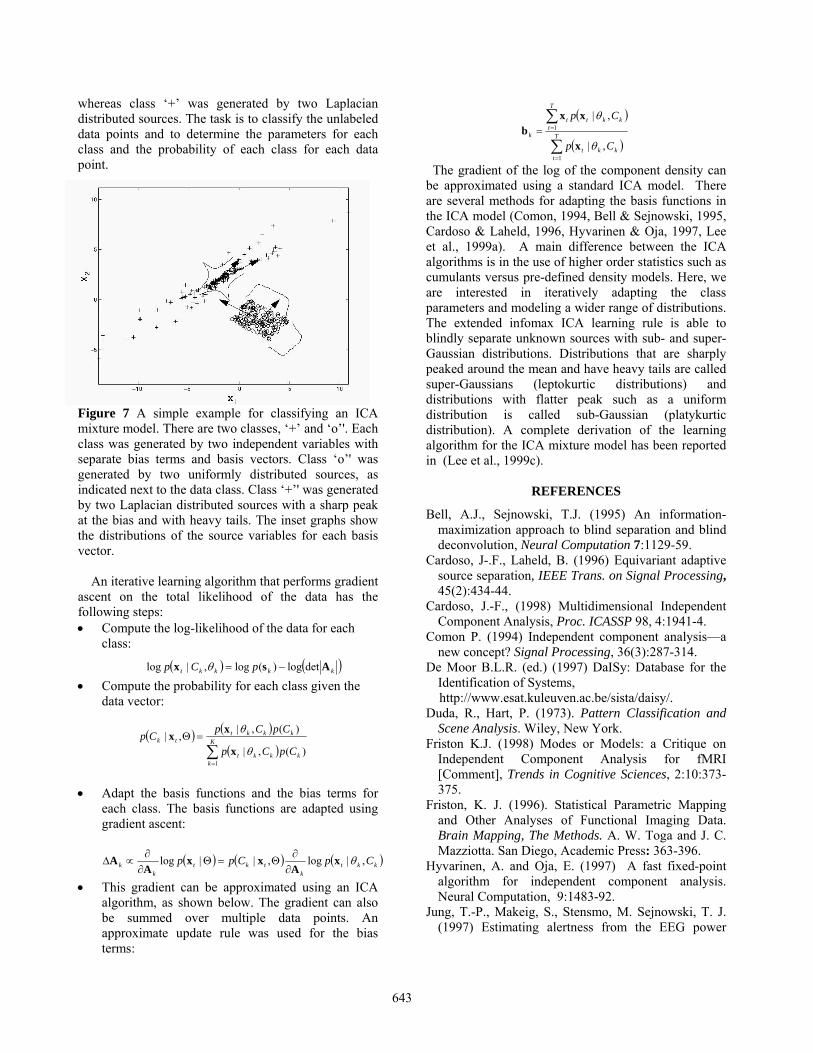
whereas class ‘+’ was generated by two Laplacian distributed sources. The task is to classify the unlabeled data points and to determine the parameters for each class and the probability of each class for each data point.

Figure 7 A simple example for classifying an ICA mixture model. There are two classes, ‘+’ and ‘o’'. Each class was generated by two independent variables with separate bias terms and basis vectors. Class ‘o’' was generated by two uniformly distributed sources, as indicated next to the data class. Class ‘+’' was generated by two Laplacian distributed sources with a sharp peak at the bias and with heavy tails. The inset graphs show the distributions of the source variables for each basis vector. An iterative learning algorithm that performs gradient ascent on the total likelihood of the data has the following steps: • Compute the log-likelihood of the data for each

class:

• Compute the probability for each class given the data vector:

• Adapt the basis functions and the bias terms for

each class. The basis functions are adapted using gradient ascent:

• This gradient can be approximated using an ICA algorithm, as shown below. The gradient can also be summed over multiple data points. An approximate update rule was used for the bias terms:

The gradient of the log of the component density can be approximated using a standard ICA model. There are several methods for adapting the basis functions in the ICA model (Comon, 1994, Bell & Sejnowski, 1995, Cardoso & Laheld, 1996, Hyvarinen & Oja, 1997, Lee et al., 1999a). A main difference between the ICA algorithms is in the use of higher order statistics such as cumulants versus pre-defined density models. Here, we are interested in iteratively adapting the class parameters and modeling a wider range of distributions. The extended infomax ICA learning rule is able to blindly separate unknown sources with sub- and super-Gaussian distributions. Distributions that are sharply peaked around the mean and have heavy tails are called super-Gaussians (leptokurtic distributions) and distributions with flatter peak such as a uniform distribution is called sub-Gaussian (platykurtic distribution). A complete derivation of the learning algorithm for the ICA mixture model has been reported in (Lee et al., 1999c).

REFERENCES

Bell, A.J., Sejnowski, T.J. (1995) An information-maximization approach to blind separation and blind deconvolution, Neural Computation 7:1129-59.

Cardoso, J-.F., Laheld, B. (1996) Equivariant adaptive source separation, IEEE Trans. on Signal Processing, 45(2):434-44.

Cardoso, J.-F., (1998) Multidimensional Independent Component Analysis, Proc. ICASSP 98, 4:1941-4.

Comon P. (1994) Independent component analysis—a new concept? Signal Processing, 36(3):287-314.

De Moor B.L.R. (ed.) (1997) DaISy: Database for the Identification of Systems,

http://www.esat.kuleuven.ac.be/sista/daisy/. Duda, R., Hart, P. (1973). Pattern Classification and

Scene Analysis. Wiley, New York. Friston K.J. (1998) Modes or Models: a Critique on

Independent Component Analysis for fMRI [Comment], Trends in Cognitive Sciences, 2:10:373-375.

Friston, K. J. (1996). Statistical Parametric Mapping and Other Analyses of Functional Imaging Data. Brain Mapping, The Methods. A. W. Toga and J. C. Mazziotta. San Diego, Academic Press: 363-396.

Hyvarinen, A. and Oja, E. (1997) A fast fixed-point algorithm for independent component analysis. Neural Computation, 9:1483-92.

Jung, T.-P., Makeig, S., Stensmo, M. Sejnowski, T. J. (1997) Estimating alertness from the EEG power

( ) ( )kkkkt pCp Asx detlog)(log,|log −=θ

( ) ( )

( )∑=

=Θ K

kkkkt

kkkttk

CpCp

CpCpCp

1

)(,|

)(,|,|

θ

θ

x

xx

( ) ( ) ( )kktk

tktk

k CpCpp ,|log,||log θxA

xxA

A∂∂

Θ=Θ∂∂

∝∆

( )

( )∑

∑

=

== T

tkkt

T

tkktt

k

Cp

Cp

1

1

,|

,|

θ

θ

x

xxb

644

spectrum, IEEE Transactions on Biomedical Engineering 44(1), 60-9.

Jung, T-P., Makeig, S., Bell, A.J., Sejnowski, T. J. (1998) Independent component analysis of electroencephalographic and event-related potential data, In: Poon & Brugge(Ed), Auditory Processing and Neural Modeling, Plenum Press, 160-88.

Jung, T. -P., Makeig, S., Townsend, J., Westerfield, M., Hicks, B., Courchesne, E., and Sejnowski, T. J., (1999a). Single-trial ERPS during continuous fMRI scanning, Society for Neuroscience Abstract 25, 1389

Jung T-P, Makeig S, Westerfield M, Townsend J, Courchesne E, and Sejnowski TJ, (1999b) Analyzing and Visualizing Single-trial Event-related Potentials, In: Advances in Neural Information Processing Systems 11:118-24.

Jung T-P, Humphries C., Lee T-W, McKeown M.J., Iragui V., Makeig S., Sejnowski T.J., (2000) Removing Electroencephalographic Artifacts from by Blind Source Separation, Psychophysiology 37:163-78.

Kobayashi K, James CJ, Nakahori T, Akiyama T, Gotman J (1999). solation of epileptiform discharges from unaveraged EEG by independent component analysis, Clin Neurophysiol. 110(10):1755-63.

Lee, T.-W., Girolami, M., Sejnowski, T.J. (1999a) Independent component analysis using an extended infomax algorithm for mixed sub-Gaussian and super-Gaussian sources, Neural Computation 11(2): 609-633.

Lee, T.-W., Lewicki, M.S. and Sejnowski, T.J. (1999b) A Mixture Models For Unsupervised Classification And Automatic Context Switching, International Workshop on Independent Component Analysis (ICA’99), 209-214.

Lee, T.-W., Lewicki, M.S., Sejnowski, T.J. (1999c) Unsupervised Classification with non-Gaussian Mixture Models using ICA, Advances in Neural Information Processing Systems 11: 508-514.

Lee, T.-W., Lewicki, M.S., Sejnowski, T.J. Unsupervised Classification with non-Gaussian Sources and Automatic Context Switching in Blind Signal Separation, IEEE Transactions on Pattern Analysis and Machine Intelligence (in press)

Makeig, S., Bell, A.J., Jung, T-P., Sejnowski, T.J. (1996) Independent component analysis of Electroencephalographic data, In: Advances in Neural Information Processing Systems 8:145-151.

Makeig S., Inlow, M. (1993) Lapses in alertness: Coherence of fluctuations in performance and EEG spectrum. Electroencephalogr. Clin. Neurophysiol. 86:23-35.

Makeig, S., Jung, T-P., Ghahremani, D., Bell, A.., Sejnowski, T. J. (1997) Blind separation of auditory event-related brain responses into independent components, Proc Natl Acad Sci USA 94:10979-84.

Makeig, S., Westerfield, M., Jung, T.-P., Covington, J., Townsend, J., Sejnowski, T. J. Courchesne, E. (1999), Functionally Independent Components of the Late Positive Event-Related Potentials during Visual Spatial Attention, Journal of Neurosciences 19(7): 2665-80.

Makeig, S., Jung, T.-P., Ghahremani, D., and Sejnowski, T. J., Independent component analysis of simulated ERP data, In: T. Nakada (Ed.) Human Higher Function I: Advanced Methodologies, (in press-a).

Makeig S, Enghoff S, Jung T-P, and Sejnowski TJ, A Natural Basis for Efficient Brain-Actuated Control, IEEE Trans Rehab Eng, (in press-b).

McKeown, M. J. (2000). Detection of consistently task-related activations in fMRI data with HYBrid Independent Component Analysis (HYBICA). NeuroImage 11: 24-35.

McKeown, M., Humphries, C., Iragui, V., Sejnowski, T.J. Spatially Fixed Patterns Account for the Spike and Wave Features in Absence Seizures. Brain Topography: (in press).

McKeown, M. J., Jung, T-P, Makeig, S., Brown, G.G., Lee, T-W, Kindermann, S.S., Sejnowski, T.J. (1998). Spatially independent activity patterns in functional MRI data during the stroop color-naming task. Proceedings of the National Academy of Sciences of the United States of America 95(3): 803-10.

McKeown, M. J., Makeig, S., Brown, G.G., Jung, T-P, Kindermann, S.S., Bell, A.J., Sejnowski, T.J. (1998). Analysis of fMRI data by blind separation into independent spatial components, Human Brain Mapping 6(3): 160-88.

McKeown, M. J., Sejnowski, T.J. (1998). Independent Component Analysis of fMRI Data: Examining the Assumptions. Human Brain Mapping 6: 368-372.

McKeown, M. J., Makeig, S., Brown, G.G., Jung, T-P, Kindermann, S.S., Bell, A.J., Sejnowski, T.J. (1998). Response from Martin McKeown, Makeig, Brown, Jung, Kindermann, Bell and Sejnowski [Comment] Trends in Cognitive Sciences, 1998, 2:10:375.

Petersen, K., Hansen, L., Kolenda, T., Rostrup, E., and Strother, S. (2000) On the independent components of functional neuroimages., ICA-2000, Helsinki, Finland, June 22, 2000.

Schoener, H., Stetter, M., Schießl, I., Lund, J. McLoughlin, N. Mayhew, J.E.W., Obermayer, K. (2000) Application of blind separation of sources to optical recording of brain activity Advances in Neural Information Processing Systems 12.

Vigario, R., Oja, E. (1999) Independent component analysis of human brain waves. In: Engineering Applications of Bio-Inspired Artificial Neural Networks. Int’l Work-Conference on Artificial and Natural Neural Networks (IWANN'99) 2:238-47.