Independent component analysis and nongaussianity for

Integrated Computer-Aided Engineering 15 (2008) 219–2 219IOS Press

Independent component analysis andnongaussianity for blind image deconvolutionand deblurring

Hujun Yin and Israr HussainSchool of Electrical and Electronic Engineering, The University of Manchester, Manchester M60 1QD, UKE-mail: [email protected], [email protected]

Abstract. Blind deconvolution or deblurring is a challenging problem in many signal processing applications as signals andimages often suffer from blurring or point spreading with unknown blurring kernels or point-spread functions as well as noisecorruption. Most existing methods require certain knowledge about both the signal and the kernel and their performance dependson the amount of prior information regarding the both. Independent component analysis (ICA) has emerged as a useful methodfor recovering signals from their mixtures. However, ICA usually requires a number of different input signals to uncover themixing mechanism. In this paper, a blind deconvolution and deblurring method is proposed based on the nongaussianity measureof ICA as well as a genetic algorithm. The method is simple and does not require prior knowledge regarding either the imageor the blurring process, but is able to estimate or approximate the blurring kernel from a single blurred image. Various blurringfunctions are described and discussed. The proposed method has been tested on images degraded by different blurring kernelsand the results are compared to those of existing methods such as Wiener filter, regularization filter, and the Richardson-Lucymethod. Experimental results show that the proposed method outperform these methods.

1. Introduction

Signals and images often suffer from degradationdue to imperfection in the capturing and imaging pro-cess; therefore a recorded signal/image is inevitablya degraded version of the original signal/image. Forinstance, recorded neuronal activities (action poten-tials or local field potentials) are often mixed activitiesof several neurons or a population; satellite/aerial im-ages usually suffer from degradation from atmosphericturbulence and lens defocusing. In addition to theseblurring effects, noise may corrupt any recorded im-age/signal. It can be introduced into the system bythe creating medium or by the recording medium orsimply because of the measurement precision. Undo-ing these imperfections is crucial for many image pro-cessing and multidimensional signal processing tasks.For most signal reconstruction methods, the character-istics of the degrading system and the noise need to beknown or are often assumed to be known a priori. Then

the restoration process may become straightforward oreven trivial. However, this information is not alwaysavailable for various reasons. Therefore the reconstruc-tion requires not only restoration of the image/signalbut also estimation of the blurring parameters from thedegraded image/signal – the procedure is often referredto as blind deconvolution.

Blind deconvolution is not a new area and there ex-ist several approaches and methods [1,2,4,8]. For in-stance, an automatic image deblurring algorithm basedon an adaptive Gaussian model has been proposed andit has been shown robust and to yield satisfactory re-sults on high resolution satellite data [7]. However, it islimited in the sense that it is based on Gaussian modelsand works mainly on satellite images. In [11] an algo-rithm for blind restoration of blurred and noisy imageswas proposed; the technique involves two processingblocks, one for denoising using the singular value de-composition and compression filtering, and one for de-blurring based on a double regularization technique.It has been demonstrated that this technique is effec-

ISSN 1069-2509/08/$17.00 © 2008 – IOS Press and the author(s). All rights reserved

220 H.Yin and I. Hussain / ICA and nongaussianity for blind image deconvolution and deblurring

tive in restoring severely blurred and noise-corruptedimages without exact knowledge of either the noise orimage characteristics. This method, however, is notcompletely blind. It requires certain prior informationon the image degradation function to implement the al-gorithm. An exhaustive list of typical methods for im-age restoration and identification can be found in [9]; afew more methods such as the Richardson-Lucy and itsvariants are described in [3,10,13,16]. These previoustechniques are limited in the sense that they are eitherdomain specific, i.e. for a particular category of imagesor particular type of degrading functions, or requirecertain prior knowledge about the point spread function(PSF), the image and/or the noise.

The motivation of this work is to derive an effectiveand efficient method based on nongaussianity measuresof independent component analysis (ICA), in order toperform a completely blind deblurring or deconvolutionwith or without the presence of noise. ICA has beenpredominantly used for 1-D signals such as speech andEEG signal processing; and it usually requires multi-ple observed signals. Applying to blind deconvolution,especially on a single blurred image/signal is a chal-lenging task. A recent approach has been proposedin [14]. It applies ICA on neighbouring shifted subimages to extract the original images and its deriva-tives [14]. However, the assumption that the originalimage and its derivatives are statistically independentmay not be valid, especially when blurring is mediumto severe. Experimental results of only weak blurringhave been reported. In this paper a different approach isproposed using ICA principle and associated nongaus-sianity measures. The proposed method requires noprior knowledge about image, noise and blurring func-tions and is based on single blurred image. Althoughthis paper focuses on deblurring image, the proposedblind deconvolution method is applicable to other sig-nals in general. A preliminary result on 1-D signalsand images has been reported in [17]. There exist manytypes of degradation function such as misfocus,motion,or atmospheric turbulence. The proposed method cancater to the degradation caused by any kind of blurringfunction.

The layout of the paper is as follows. The conceptsrelated to ICA and nongaussianity measures for decon-volution and deblurring are explained in the next Sec-tion. Then in Section 3, the proposed method is de-scribed in detail with the experimental setups, togetherwith the results on various degradation functions andcomparisons with the existing methods. The discus-sions and conclusions are given in Section 4.

2. ICA and Nongaussianity for Deblurring

A blurred image can be modelled as the convolutionof an original image with a 2-D blurring kernel or point-spread function (PSF) with or without a noise term,

x(i, j) = f(i, j) ⊗ b(i, j) + η(i, j) =m∑

k=−m

n∑l=−n

b(k, l)f(i + k, j + l) + η(i, j), (1)

where ⊗ denotes the convolution operator, x(i, j) isthe degraded image, f(i, j) is the original image; b(k,l) is the PSF; η(i, j) is the added noise; and m and nare the effective ranges of the blurring kernel on i andj axes, respectively.

The PSFs under consideration and experimentedhere are not functions of spatial location; in otherwords, they are spatially invariant, though the proposedtechnique can, in principle, be extended to deal withspatially variant blurring. Essentially, this means thatthe image is blurred in exactly the same way at everyspatial location.

In blind deconvolution, a convoluted version x ofan original signal f is observed, without knowing ei-ther the signal f or the convolution kernel b [12,14].The problem is then to find a deblurring filter h so thatf = h⊗x; this is often an ill-posed mathematical prob-lem. The equalizer or deblurring filter h is assumed tobe or realized as a FIR filter of sufficient length, so thatthe truncation effect can be ignored. A special case ofblind deconvolution that is especially interesting is thecase where it is assumed that the values of the signalf at two different points of space are statistically inde-pendent. Under certain assumptions, this problem canbe solved by simply whitening the observed signal x.However, to solve the problem in full, one must assumethat the signal f is non-Gaussian, and use higher-orderinformation [5,6]. Thus the techniques used for solv-ing this special case of the problem are very similarto those used in other higher-order methods like ICA.ICA is a technique that recovers a set of independentsignals from a set of observed mixed signals without apriori knowledge of the sources, and is also closely as-sociated to blind source separation (BSS). It is assumedthat each observed signal is a linear combination of theindependent source signals, and that the mixing mecha-nism is generally not known. The independency of thesources makes it possible for subsequent application ofICA to recover original source signals.

Further, the distributions of the source signals areassumed to be unknown, except that they may not be

H. Yin and I. Hussain / Independent component analysis and nongaussianity for blind image deconvolution and deblurrin 221

Gaussian, or at most only one source can be Gaussian.Basic working methodology behind such a scheme is tolook for nongaussianity in the recovered signals. Thereis a clear link between ICA and blind deconvolution;more precisely blind deconvolution is a special case ofICA where the original signals are i.i.d over space (ortime in 1-D case). In blind deconvolution, we have on-ly one observed signal (output) and one source (input).The observed signal consists of an unknown source sig-nal mixed with itself at different spatial locations (ortime delays in 1D case). This could be due to echoescaused by the reverberating nature of the environmentor degradations as mentioned before. The task is to es-timate the source signal from the observed signal only,without knowing the mixing or convolving system, thetime delays, or the mixing coefficients.

From the Central Limit Theorem (CLT), we knowthat the output of a linear system tends to be moreGaussian. ICA tries to find a solution that maximizesthe “nongaussianity” of the recovered signal. Becauseof that, the technique does not usually work with Gaus-sian signals, since their higher cumulants are equal tozero. The CLT implies that if we can find a combi-nation of the measured signals with minimal Gaussianproperties, then that signal will be one of the indepen-dent signals. In order to do this a way to measurenongaussianity is required.

Kurtosis is a classical method for measuring non-gaussianity. When data is pre-processed to have unitvariance, kurtosis is related to the fourth moment ofthe data. In an intuitive sense, kurtosis measures how“spikiness” of a distribution or the size of the tails.Kurtosis is simple to calculate; however, it is sensitiveto outliers in the data set. Its values may be dominatedby only few values in the tails, which means that itsstatistical significance is poor. Mathematically kurtosisis defined as

Kurt(y) = E{y4} − 3(E{y2})2. (2)

In cases where y has unit variance, Kurt(y) =E{y4} − 3. In other words, kurtosis is a normalizedversion of the fourth moment. It is zero for Gaussianvariables and is greater or smaller than zero for super-or sub-Gausian variables, respectively. Often the abso-lute value of kurtosis is used to measure the nongaus-sianity. As kurtosis is sensitive to outliers and noise, inmany situations there is need for a more robust measureof nongaussianity. Negentropy is the one and is oftenused for this purpose. Unlike kurtosis, the negentropyis robust but computationally complex. In practice itcan only be approximated.

Negentropy is based on the information theoreticquantity of differential entropy, or simply entropy as itis often called. The entropy of a random variable isrelated to the information that the observation of thevariable gives. The more unpredictable and unstruc-tured the variable is, the larger the entropy. As a re-sult Gaussian variable has the largest entropy; all otherstructured or clustered data sets have entropy less thanthat of the Gaussian. This very fact can be used as ameasure of nongaussianity.

A normalized version of differential entropy is usedfor obtaining a measure of nongaussianity that is ze-ro for Gaussian variable and always nonnegative forothers. This is defined as ‘negentropy’, which can bestated as

J(Y ) = H(Ygauss) − H(Y ), (3)

where H(Y ) is the (differential) entropy of the variableY and H(Ygauss) is the (differential) entropy of theGaussian variable of the same correlation (covariance)matrix as Y . Negentropy is always nonnegative and iszero for Gaussian variables. It is a robust measure ofnongaussianity; however the problem is in its estima-tion for which one requires knowledge of the pdf of thegiven variable. Therefore some approximation tech-niques will have to be used for estimating negentropy.A typical method is to use higher-order cumulants, orpolynomial expansions. This gives,

J(y) ≈ 112

E{y3}2 +148

kurt(y)2, (4)

where y is assumed to be zero mean and unit variance.However, the problem with this approximation is thatone again relies on kurtosis for measuring the nongaus-sianity. As it can be seen that the first term in Eq. (4) un-der symmetric distributions is zero, therefore one is leftwith square of kurtosis. Hence it is prone to the sameproblems of kurtosis. More sophisticated techniquesfor approximation of negentropy are required.

One way could be, to use expectations of generalnon-quadratic functions or non-polynomial moments,to replace polynomial functions ‘y 3’ and ‘y4’ by otherfunctions possibly two or more. This gives a simpleway of approximating negentropy. For a simple casethe approximation becomes [6]

J(y) ≈ k1(E{Go(y)})2 + k2(E{Ge(y)}(5)

−E{Ge(v)})2,where k1 and k2 are positive constants; v is Gaussianvariable and both y and v are of zero mean and unitvariance; Go and Ge are odd and even nonquadratic

222 H. Yin and I. Hussain / Independent component analysis and nongaussianity for blind image deconvolution and deblurring

1 2 3 4 5

-0.75

-0.65

-0.55

σ

Kurto

sis

1 2 3 4 5

-0.6

-0.5

-0.4

-0.3

σKu

rtosi

s1 2 3 4 5

-0.83

-0.81

-0.79

-0.77

σ

Kurto

sis

Fig. 1. Nongaussianity analysis for Barbra (left), Lena (middle) and Cameraman (right) images for increased blurring.

1 2 3 4 50

5

10

15

20

σ

Kur

tosi

s

1 2 3 4 5

2

6

10

14

σ

Neg

entro

py

1 2 3 4 5

0.20

0.21

0.21

0.22

σN

egen

tropy

Fig. 2. Nongaussianity analysis on deblurring Barbra image (kurtosis: Eq. (2)-left, negentropy: Eq. (4)- middle, and negentropy: Eq. (5) withfunctions of Eqs (6) and (7) – right).

functions respectively. This measure is more robustthan the one in Eq. (4). Different choices exist fornonquadratic functions. A useful choice is [6],

Go(y) =1a1

log cosh(a1y), (6)

Ge(y) = − exp(−y2

2

), (7)

where 1� a1 � 2. Thus one can obtain the negentropythat is a good compromise between the properties oftwo classic nongaussianity measures given by kurtosisand negentropy.

The above mentioned measures can be applied forfinding independency and nongaussianity in the sub-sequent deblurring process. The observed signals orimages need to be centred and normalized before ap-plying these measures. The blurring process producescorrelation between the adjacent points of the signalthus making the signal/image more Gaussian than theoriginal. Further, the stronger or wider the blurring themore the degraded signal/image moves towards Gaus-sian. Figure 1 illustrates this very fact where the non-gaussianity measure of Eq. (2) was taken on blurredimages (with a Gaussian kernel of varying width, σ)of Barbra, Lena and Cameraman respectively. Theimages become more Gaussian as the results of blur-

ring and furthermore the stronger the blurring the moreGaussian the images become.

As stated earlier, the CLT implies that the outputof a linear system is more Gaussian than the originalsignal. Therefore if one wishes to recover the origi-nal signal, it would be the one that has the minimumGaussian properties. Therefore a filter that maximizesthe nongaussianity of the mixed/degraded signal wouldbe the inverse filter (if it exists) of the original blurringfilter. An optimization process can be performed onthese nongaussianity measures. Then adaptive learn-ing rules can be obtained for estimating iteratively thedeblurring filter parameters W , the inverse of the blur-ring filter. Following [6], a gradient-based learning al-gorithms can be obtained based on either kurtosis ornegentropy measure,

∆W ∝ sign(Kurt(W⊗X))E{X(W ⊗ X)3},(8)

∆W ∝ (E{G(W ⊗ X)} − E{G(v)})(9)

E{Xg(W ⊗ X)},where G is a nonquadratic function and g is the deriva-tive of G and v is a standardized Gaussian randomvariable. Eq. (9) is derived from a simplified case ofnegentropy measure of Eq. (5), where only the secondterm is considered.

H. Yin and I. Hussain / Independent component analysis and nongaussianity for blind image deconvolution and deblurring 223

1 2 3 4 5

0

2

4

6

σ

Kur

tosi

s

1 2 3 4 5

0.5

1

1.5

2

σ

Neg

entro

py1 2 3 4 5

0.21

0.21

0.21

0.22

0.22

σ

Neg

entro

py

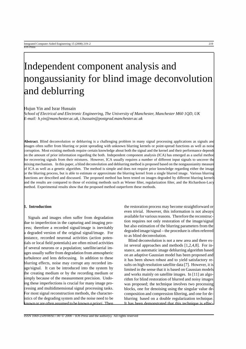
Fig. 3. Nongaussianity analysis on deblurring Cameraman image (left – kurtosis: Eq. (2); middle – negentropy: Eq. (4); and right – negentropy:Eq. (5) with functions of Eqs (6) and (7)).

510

1520

510

1520

0.01

0.030.20.6

-π/2

-π/2 -π/2

00

Fig. 4. Gaussian PSF (with σ=2) and its Fourier transform (magnitude).

Figures 2 and 3 show various nongaussianity mea-sures of a deblurring system on two images (Barbraand Cameraman). Both images have been blurred witha Gaussian PSF. These measures are kurtosis Eq. (2),and negentropy Eqs (4) and (5) respectively, on thedeblurred images of various deblurring kernel width.

It is worthwhile to mention here that the above non-gaussianity analysis is not only true for Gaussian blur-ring filter but also for other point-spread functions, suchas uniform out of focus blur, atmospheric blur or mo-tion blur (see next section). Furthermore, nongaussian-ity analysis can be used to find and optimize the blur-ring filter and its parameters, e.g. Eqs (8) and (9), thuspaving the way for estimation of the degrading filterand thus the blind deconvolution of the signal. Howev-er as shown in Figs 2 and 3, the gradient based methodscan be easily trapped in local minima.

3. Proposed method and experimental results

In this Section, we present a blind image deconvolu-tion and deblurring approach based on nongaussianitymeasures and genetic algorithms. The method makesuse of the difference between blurred (correlated) and

un-blurred (original) images, using the very fact of theCLT. Therefore the original image can be recovered us-ing a nongaussianity measure as ICA and BSS use tofind independent components and to separate the sig-nals. Here the nongaussianity measure is used to dif-ferentiate between the correlated, blurred image andthe uncorrelated image; the restored image is more in-dependent (or uncorrelated) than the blurred one. Theblurring type and parameters of the estimated PSF areoptimized a genetic algorithm in an iterative manner.The operation is conducted in the spatial frequency do-main. The approach is computationally simple and effi-cient. The process can be summarized in the followingsteps:

1. Initialize the genetic algorithm parameters: en-coding bits (e.g. 16 bits), population size (e.g.2000), crossover rate (e.g. 0.25), mutation rate(0.005), etc.

2. Calculate the nongaussianity of the blurred imageand Fourier coefficients of the blurred image.

3. Perform one iteration for different types and val-ues of the blurring kernel parameters; find the re-stored image through inverse/wiener filtering inthe spectral domain based on the current estimate


Fig. 5. Degraded Cameraman image with Gaussian blurring (σ = 3) and restored with the proposed method (estimated σ = 2.91).

24

68

10

24

68

10

0.0050.01 0.5

1

-π/2

0 0

π/2 π/2

Fig. 6. PSF of uniform out of focus (circular) blur (with R=5) and its Fourier transform (magnitude).

of the kernel function. Convert the image to spa-tial domain and calculate its nongaussianity fordifferent population samples.

4. Generate the child population for next iteration byevolving from the parents on the basis of the fittestfunction (that is, the nongaussianity measure),and optimize the fitness function in subsequentiterations (generations).

5. Go back to Step (3) till a convergence criterion ismet or a pre-set maximum number of generation(e.g. 50) is reached.

The proposed method is computationally simple andeasy to implement. It can be applied for estimation ofthe parameters of the blurring filter such as the spread ofGaussian blurring filter or length of motion in the caseof motion blur. Furthermore, different PSFs are appliedfor the blind deconvolution of the blurred images withand without noise. The proposed algorithm has beentested on various image degradation functions.

3.1. Atmospheric turbulence Blur

Atmospheric turbulence is a severe limitation in re-mote sensing. Although the blur introduced by at-

mospheric turbulence depends on a variety of factors(such as temperature, wind speed, exposure time), forlong-term exposures the point-spread function can bedescribed reasonably well by a Gaussian function:

b(i, j; σ) = C exp(− i2 + j2

2σ2

). (10)

Here σ determines the amount of spread of the blurring,and the constant Cis to be chosen so that energy conser-vation rule is satisfied. The discrete version of Eq. (10)is usually obtained by numerical discretization of thecontinuous PSF for each element. Since the spatiallycontinuous PSF does not have a finite support, it hasto be truncated properly. Figure 4 shows such a PSFand its similar shape in the spectral domain (with σ =2). Note that Gaussian blurs do not have exact spectralzeros.

The proposed method has been applied for deblur-ring images of atmospheric (Gaussian) blurring. Fig-ure 5 displays the result for the Cameraman image: theblurred image (blurred with Gaussian PSF with σ = 3)and the estimated, blind-deblurred image by the pro-posed method. The estimated blurring parameter isσ = 2.91).


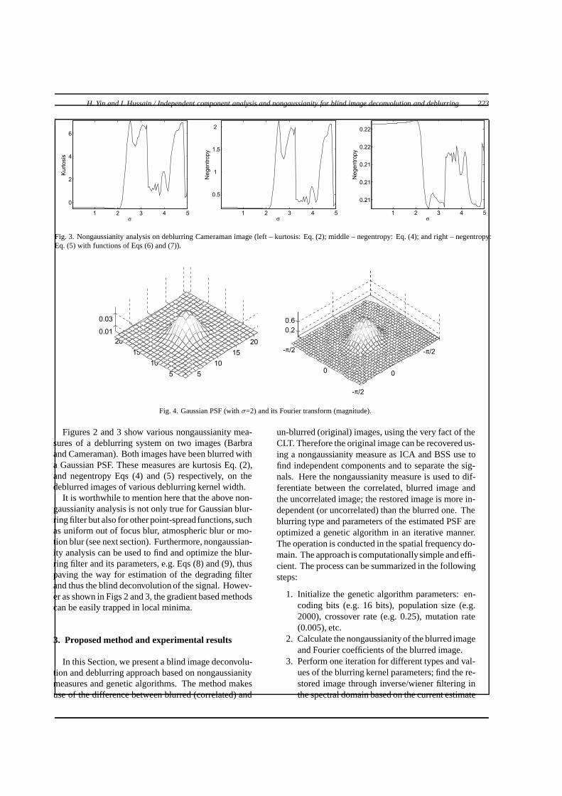
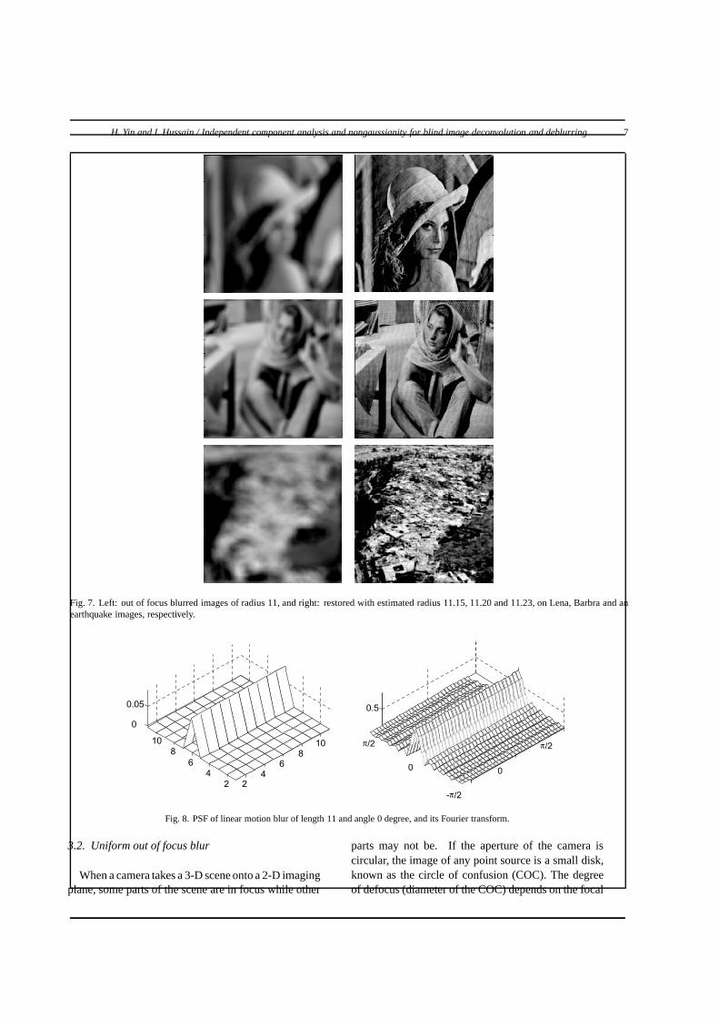
Fig. 7. Left: out of focus blurred images of radius 11, and right: restored with estimated radius 11.15, 11.20 and 11.23, on Lena, Barbra and anearthquake images, respectively.

24

68

10

24

68

10

0

0.05 0.5

-π/2

0

π/2π/2

0

Fig. 8. PSF of linear motion blur of length 11 and angle 0 degree, and its Fourier transform.

3.2. Uniform out of focus blur

When a camera takes a 3-D scene onto a 2-D imagingplane, some parts of the scene are in focus while other

parts may not be. If the aperture of the camera iscircular, the image of any point source is a small disk,known as the circle of confusion (COC). The degreeof defocus (diameter of the COC) depends on the focal


Table 1PSNR comparison of the proposed method with other techniques. Note that in Wiener and Regularised filters and bothRichardson-Lucy methods, the true PSF was supplied as the initial PSF. So their results can only be interpreted the upperlimits. When a random initial PSF was used they do not converge to good results

PSNR (dB)Blurring Blurred and Wiener filter Regularized Richardson- Blind Richardson- Proposedwidthσ noisy image filter Lucy method Lucy method method

Barbra 2 23.56 23.72 23.72 23.40 22.96 24.083 22.82 23.01 23.01 23.46 23.36 23.684 22.23 22.41 22.41 23.19 23.17 23.335 21.81 21.99 21.98 22.87 22.86 22.97

Lena 2 27.68 28.01 28.01 27.83 27.03 29.633 25.66 25.66 25.66 27.72 27.56 28.024 24.40 24.57 24.57 26.78 26.74 26.975 23.61 23.76 23.76 25.70 25.70 25.93

Boat 2 25.71 25.64 25.64 26.82 26.28 27.423 23.87 23.75 23.75 25.95 25.87 26.014 22.81 22.73 22.73 24.77 24.77 23.805 22.16 22.14 22.14 23.71 23.71 22.73

Zelda 2 30.91 32.13 32.13 28.37 25.85 32.853 29.06 30.09 30.09 29.72 28.70 31.404 27.83 28.69 28.69 29.63 29.25 30.425 26.99 27.81 27.81 28.96 28.80 29.47

length, the aperture value of the lens, and the distancebetween the camera and object. An accurate modelwould describe the diameter of the COC and provide theintensity distribution within the COC. However, if thedegree of defocusing is large relative to the wavelengthsconsidered, a geometrical approach can be followed –resulting in a uniform intensity distribution within theCOC. The spatially continuous PSF of this uniformout-of-focus blur with radius Ris given by:

b(i, j; R) ={

1CπR2 if

√i2 + j2 � R2

0 elsewhere, (11)

where Cis a constant that must be chosen so that en-ergy conservation law is satisfied. The approximationof Eq. (11) is incorrect for the fringe elements of thepoint-spread function. A more accurate model for thefringe elements would involve the integration of thearea covered by the spatially continuous PSF that needsto be calculated by integration. Figure 6(a) shows theprofiles of such a PSF and its Fourier transform.

Figure 6(b) shows the modulus of the Fourier trans-form of this type of PSF for R = 5. Again a low passbehaviour can be observed (in this case both horizontal-ly and vertically), as well as a characteristic pattern ofspectral zeros. Figure 7 displays the results of applyingthe proposed method on this type of burring. Here theoriginal images were blurred with uniform out of focusblur of radius 11. The proposed method was applied tooptimize the parameters of the deblurring function byusing kurtosis as the nongaussianity measure.

Fig. 9. Left: linear motion blurred images of length 11 and angle45 degree, and right: restored images with estimated length of linearblur being 11.1 and 11.24 for Lena and Barbra, respectively.

3.3. Linear motion blur

Many types of motion blur are due to relative motionbetween the recording device and the scene. This can bein the form of a translation, a rotation, a sudden changeof scale, or some combination of these. Here only theimportant case of a global translation is considered.When the scene to be recorded translates relative tothe camera at a constant velocity under an angle of ϕ


Fig. 10. Blurred and noisy Barbra image (top left), processed with the proposed method (top middle), the Richardson-Lucy (top right), Regularizedfilter (bottom left), Wiener Filter (bottom middle) and the Blind Richardson Lucy method (bottom right).

Fig. 11. Blurred and noisy Lena images (top left), processed with the proposed method (top middle), processed with Richardson Lucy (to right),processed with Regularized filter (bottom right), processed with Wiener Filter (bottom middle) and processed with Blind Richardson Lucy method(bottom right).

radians with the horizontal axis during the exposureinterval, the distortion is one-dimensional. Denotingthe length of motion by L, the PSF is given by:

b(i, j; L, ϕ) =

⎧⎨⎩

1L if

√i2 + j2 � L

2 and ij

= − tanϕ0 elsewhere

.(12)

Figure 8 shows the PSF of Eq. (12) for linear motionfor length of 11 and angle of zero with the horizontaldirection and its Fourier transform (magnitude).

The proposed method has been tested to estimate theblurring parameters for the subsequent deblurring by

this PSF. In this case there are two parameters that areneeded to be optimized, the length of motion and theangle of motion. In Fig. 9, results are shown for thedegraded images and deblurring results.

3.4. Deblurring and denoising

The proposed method can also be extended to includedenoising capability. The blurred and noisy (for exam-ple, by additive white Gaussian noise) image becomesmore Gaussian compared to the original image. That is,its kurtosis or negentropy becomes more Gaussian as a


result of the blurring and adding noise. Wiener filter-ing can be used to denoise and deblur the image; whilethe proposed algorithm is used to estimate the requiredparameters of the blurring PSF and the noise. Thealgorithm is able to approximate the parameters andsubsequently to denoise and deblur the image. Typicalresults of such experiments are shown in Figs 10 and11, where images were blurred with Gaussian blurringfunction and then added with Gaussian white noise.

A comparison of the proposed method with otherexisting techniques (such as Wiener filter, regularizedfilter, Richardson-Lucy method and blind RichardsonLucy method) has been carried out on several bench-mark images such as Barbra, Lena, Boat and Zelda.They were evaluated on both qualitatively visual quali-ty and PSNR (peak signal-noise ratio) measures. PSNRperformances on these images are given in Table 1. Theproposed method produces markedly superior resultsnot only in terms of improved visual quality but alsoin quantitative PSNR terms over the existing methods.Note that the true PSF was supplied to the Wiener fil-ter, regularization filter and the Richardson-Lucy tech-niques as they are not blind methods. Even for theblind Richardson-Lucy method, it requires good a pri-ori knowledge of the PSF as the initial estimate (thetrue PSF was used in this case). The proposed blindmethod however operates in a truly blind manner andstill outperforms these existing methods in almost allcases.

4. Conclusions

A new method based on ICA, nongaussianity mea-sures and genetic algorithms for blind deconvolutionand deblurring of signals and images has been pro-posed. The proposed method is computationally sim-ple and easy to implement in practice and most impor-tant of all, it is completely blind and works on a singleimage. The method is conducted in spectral domainwhere nongaussianity analysis and genetic algorithmare used for optimizing the parameters of the candidatedegrading functions. The method does not require anya priori knowledge about either the image or the blur-ring function. The proposed method has been testedon a number of images blurred with various PSFs withand without additive noise. The results indicate thatthe proposed method is able to deblur images effective-ly. A comparison with the existing deconvolution anddeblurring methods shows the superior performance ofthe proposed blind method over the others even when

prior knowledge of the PSF is given to these methods.Future endeavours are to tackle heavy noise and ro-bustness against outliners as well as to improve on theefficiency of the parameter optimization processes.

Acknowledgement

We would like to thank anonymous reviewers fortheir helpful and constructive comments, which havehelped the revision of the paper enormously.

References

[1] G.R. Ayers and J.C. Dainty, Iterative blind deconvolutionmethod and its applications, Optics Letters 13 (1988), 547–549.

[2] M.R. Banham and A.K. Katsaggelos, Digital image restora-tion, IEEE Signal Processing Magazine 14(2) (1997), 24–41.

[3] D.A. Fish, A.M. Brinicombe, E.R. Pike and J.C. Walker, Blinddeconvolution by means of the Richardson-Lucy algorithm,Journal of the Optical Society of America A 12 (1995), 58–65.

[4] R.C. Gonzalez and R.E. Woods, Digital Image Processing,Prentice Hall, 2002.

[5] A. Hyvarinen, Survey on independent component analysis,Neural Computing Surveys 2 (1999), 94–128.

[6] A. Hyvarinen, J. Karhunen and E. Oja, Independent Compo-nent Analysis, John Willey & Sons, 2001.

[7] A. Jalobeanu, L.B. Feraud and J. Zerubia, An adaptive Gaus-sian model for satellite image deblurring, IEEE Trans. ImageProcessing 13 (2004), 613–621.

[8] D. Kundur and D. Hatzinakos, Blind image deconvolution,IEEE Signal Processing Magazine 13(3) (1996), 43–64.

[9] R.L. Lagendijk and J. Biemond, Basic methods for imagerestoration and identification, in: Handbook of Image andVideo Processing, A.C. Bovik and J.D. Gibson, eds, 2000.

[10] L.B. Lucy, An iterative technique for the rectification of ob-served images, Astronomical Journal 79 (1974), 745–754.

[11] N. Moayeri and K. Konstantinides, An Algorithm forblind restoration of blurred and noisy images, Hewlett-Packard Labs Technical Report HPL-96-102, available athttp://www.hpl.hp.com/techreports.

[12] T.F. Rabie, R.M. Rangayyan and R.B. Paranjape, Adaptive-neighborhood image deblurring, Journal of Electronic Imag-ing 3 (1994), 368–378.

[13] W.H. Richardson, Bayesian-based iterative method of imagerestoration, Journal of the Optical Society of America 62(1972), 55–59.

[14] S. Umeyama, Blind deconvolution of blurred images by useof ICA, Electronics and Communications in Japan Part III,84 (2001), 1–9.

[15] C. Vural and W.A. Sethares, Blind Deconvolution of NoisyBlurred Images Via Dispersion Minimization, 14th IEEE Int.Conf. on Digital Signal Processing, Santorini, Greece, 2002.

[16] R.L. White, Image restoration using the damped Richardson-Lucy method, in: The Restoration of HST Images and Spec-tra – II, R.J. Hanisch and R.L. White, eds, 1994.

[17] H. Yin and I. Hussain, ICA and Genetic Algorithms for lindSignal and Image Deconvolution and Deblurring, Proc. Inter-national Conference on intelligent Data Engineering and Au-tomated Learning (IDEAL’06), LNCS-4224, 2006, 595–603.

Documents

Independent component analysis and nongaussianity for