Embed Size (px)
Citation preview

Independent component analysis:An introduction
Alaa TharwatFaculty of Computer Science and Engineering,
Frankfurt University of Applied Sciences, Frankfurt am Main, Germany
AbstractIndependent component analysis (ICA) is a widely-used blind source separation technique. ICA has beenapplied to many applications. ICA is usually utilized as a black box, without understanding its internal details.Therefore, in this paper, the basics of ICA are provided to show how it works to serve as a comprehensivesource for researchers who are interested in this field. This paper starts by introducing the definition andunderlying principles of ICA. Additionally, different numerical examples in a step-by-step approach aredemonstrated to explain the preprocessing steps of ICA and the mixing and unmixing processes in ICA.Moreover, different ICA algorithms, challenges, and applications are presented.
Keywords Independent component analysis (ICA), Blind source separation (BSS), Cocktail party problem,
Principal component analysis (PCA)
Paper type Original Article
1. IntroductionMeasurements cannot be isolated from a noise which has a great impact onmeasured signals.For example, the recorded sound of a person in a street has sounds of footsteps, pedestrians,etc. Hence, it is difficult to record a cleanmeasurement; this is due to (1) source signals alwaysare corrupted with a noise, and (2) the other independent signals (e.g. car sounds) which aregenerated from different sources [31]. Thus, the measurements can be defined as acombination of many independent sources. The topic of separating these mixed signals iscalled blind source separation (BSS).The term blind indicates that the source signals can beseparated even if little information is known about the source signals.
One of the most widely-used examples of BSS is to separate voice signals of peoplespeaking at the same time, this is called cocktail party problem [31]. The independentcomponent analysis (ICA) technique is one of the most well-known algorithms which are usedfor solving this problem [23]. The goal of this problem is to detect or extract the sound with asingle object even though different sounds in the environment are superimposed on oneanother [31]. Figure 1 shows an example of the cocktail party problem. In this example, twovoice signals are recorded from two different individuals, i.e., two independent source signals.
ACI17,2
222
© Alaa Tharwat. Published in Applied Computing and Informatics. Published by Emerald PublishingLimited. This article is published under the Creative Commons Attribution (CC BY 4.0) license. Anyonemay reproduce, distribute, translate and create derivative works of this article (for both commercial andnon-commercial purposes), subject to full attribution to the original publication and authors. The fullterms of this license may be seen at http://creativecommons.org/licences/by/4.0/legalcode
Publishers note: The publisher wishes to inform readers that the article “Independent componentanalysis: An introduction” was originally published by the previous publisher of Applied Computingand Informatics and the pagination of this article has been subsequently changed. There has been nochange to the content of the article. This change was necessary for the journal to transition from theprevious publisher to the new one. The publisher sincerely apologises for any inconvenience caused.To access and cite this article, please use Tharwat, A. (2020), “Independent component analysis:An introduction”, New England Journal of Entrepreneurship. Vol. 17 No. 2, pp. 222-249. The originalpublication date for this paper was 31/08/2018.
The current issue and full text archive of this journal is available on Emerald Insight at:
https://www.emerald.com/insight/2210-8327.htm
Received 24 May 2018Revised 26 August 2018Accepted 29 August 2018
Applied Computing andInformaticsVol. 17 No. 2, 2021pp. 222-249Emerald Publishing Limitede-ISSN: 2210-8327p-ISSN: 2634-1964DOI 10.1016/j.aci.2018.08.006

Moreover, two sensors, i.e., microphones, are used for recording two signals, and the outputsfrom these sensors are two mixtures. The goal is to extract original signals1 from mixturesof signals. This problem can be solved using independent component analysis (ICA)technique [23].
ICA was first introduced in the 80s by J. H�erault, C. Jutten and B. Ans, and the authorsproposed an iterative real-time algorithm [15]. However, in that paper, there is no theoreticalexplanation was presented and the proposed algorithm was not applicable in a number ofcases. However, the ICA technique remained mostly unknown till 1994, where the name ofICA appeared and introduced as a new concept [9]. The aim of ICA is to extract usefulinformation or source signals from data (a set of measured mixture signals). These data canbe in the form of images, stockmarkets, or sounds. Hence, ICAwas used for extracting sourcesignals in many applications such as medical signals [7,34], biological assays [3], and audiosignals [2]. ICA is also considered as a dimensionality reduction algorithm when ICA candelete or retain a single source. This is also called filtering operation, where some signals canbe filtered or removed [31].
ICA is considered as an extension of the principal component analysis (PCA) technique[9,33]. However, PCA optimizes the covariance matrix of the data which represents second-order statistics, while ICA optimizes higher-order statistics such as kurtosis. Hence, PCAfinds uncorrelated components while ICA finds independent components [21,33]. As aconsequence, PCA can extract independent sources when the higher-order correlations ofmixture data are small or insignificant [21].
ICA has many algorithms such as FastICA [18], projection pursuit [21], and Infomax [21].The main goal of these algorithms is to extract independent components by (1) maximizingthe non-Gaussianity, (2) minimizing the mutual information, or (3) using maximum likelihood(ML) estimation method [20]. However, ICA suffers from a number of problems such as over-complete ICA and under-complete ICA.
Many studies treating the ICA technique as a black box without understanding theinternal details. In this paper, in a step-by-step approach, the basic definitions of ICA, andhow to use ICA for extracting independent signals are introduced. This paper is divided intoeight sections. In Section 2, an overview of the definition of the main idea of ICA and itsbackground are introduced. This section begins by explaining with illustrative numericalexamples how signals are mixed to form mixture signals, and then the unmixing process ispresented. Section 3 introduces with visualized steps and numerical examples twopreprocessing steps of ICA, which greatly help for extracting source signals. Section 4presents principles of how ICA extracts independent signals using different approaches suchas maximizing the likelihood, maximizing the non-Gaussianity, or minimizing the mutualinformation. This section explains mathematically the steps of each approach. Different ICAalgorithms are highlighted in Section 5. Section 6 lists some applications that use ICA forrecovering independent sources from a set of sensed signals that result from a mixing set of
Figure 1.Example of the cocktail
party problem. Twosource signals (e.g.sound signals) are
generated from twoindividuals and then
recorded by twosensors, e.g.,
microphones. Twomicrophones mixed the
two source signalslinearly. The goal of
this problem is torecover the original
signals from the mixedsignals.
Independentcomponent
analysis
223

source signals. In Section 7, the most common problems of ICA are explained. Finally,concluding remarks will be given in Section 8.
2. ICA background2.1 Mixing signalsEach signal varies over time and a signal is represented as follows, si ¼ fsi1; si2; . . . ; siNg,where N is the number of time steps and sij represents the amplitude of the signal si atthe jth time.2 Given two independent source signals3 s1 ¼ fs11; s12; . . . ; s1Ng ands2 ¼ fs21; s22; . . . ; s2Ng (see Figure 2). Both signals can be represented as follows:
S ¼�s1s2
�¼
� ðs11; s12; . . . ; s1N Þðs21; s22; . . . ; s2N Þ
�(1)
where S∈Rp3N represents the space that is defined by source signals and p indicates thenumber of source signals.4 The source signals (s1 and s2) can be mixed as follows,x1 ¼ a3 s1 þ b3 s2, where a and b are the mixing coefficients and x1 is the first mixturesignal. Thus, the mixture x1 is the weighted sum of the two source signals (s1 and s2).Similarly, another mixture ðx2Þ can be measured by changing the distance between thesource signals and the sensing device, e.g. microphone, and it is calculated as follows,x2 ¼ c3 s1 þ d3 s2, where c and d are mixing coefficients. The two mixing coefficientsa and b are different than the coefficients c and d because the two sensing devices which areused for sensing these signals are in different locations, so that each sensor measures adifferent mixture of source signals. As a consequence, each source signal has a differentimpact on output signals. The two mixtures can be represented as follows:
X ¼�x1
x2
�¼
�as1 þ bs2cs1 þ ds2
�¼
�a b
c d
��s1s2
�¼ As (2)
where X∈Rn3N is the space that is defined by the mixture signals and n is the number ofmixtures. Therefore, simply, the mixing coefficients (a; b; c, and d) are utilized fortransforming linearly source signals from S space to mixed signals in X space as follows,S→X : X ¼ AS, where A∈Rn3p is the mixing coefficients matrix (see Figure 2) and it isdefined as:
Figure 2.An illustrative exampleof the process ofmixing signals. Twosource signals aremixed linearly by themixing matrix ðAÞ toform two new mixturesignals.
ACI17,2
224
A ¼�a b
c d
�(3)
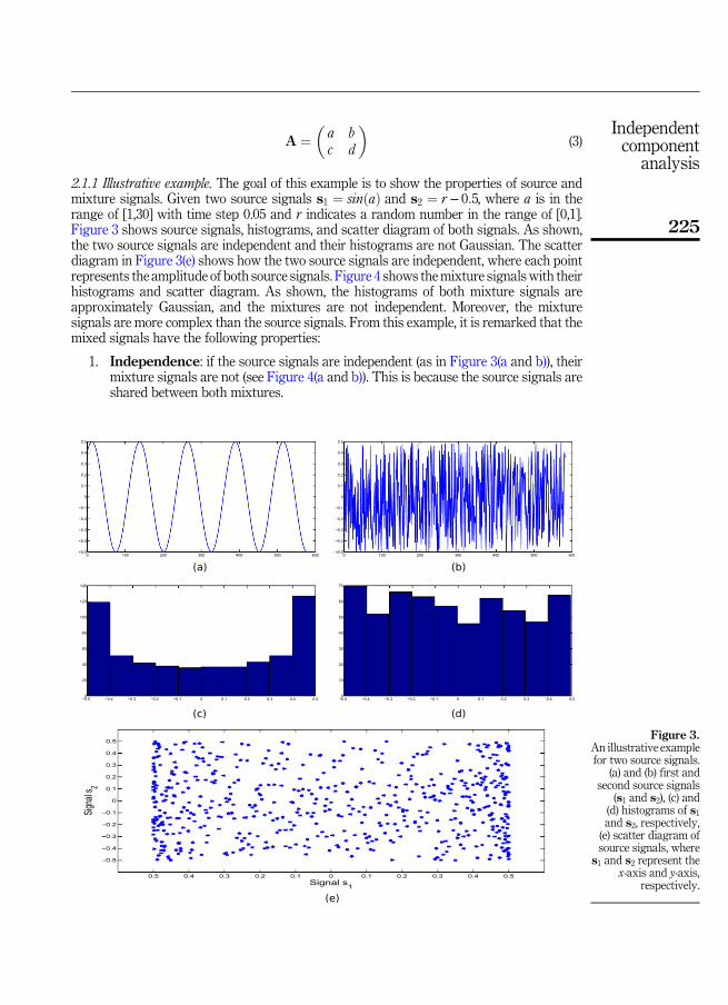
2.1.1 Illustrative example. The goal of this example is to show the properties of source andmixture signals. Given two source signals s1 ¼ sinðaÞ and s2 ¼ r− 0:5, where a is in therange of [1,30] with time step 0.05 and r indicates a random number in the range of [0,1].Figure 3 shows source signals, histograms, and scatter diagram of both signals. As shown,the two source signals are independent and their histograms are not Gaussian. The scatterdiagram in Figure 3(e) shows how the two source signals are independent, where each pointrepresents the amplitude of both source signals. Figure 4 shows themixture signals with theirhistograms and scatter diagram. As shown, the histograms of both mixture signals areapproximately Gaussian, and the mixtures are not independent. Moreover, the mixturesignals are more complex than the source signals. From this example, it is remarked that themixed signals have the following properties:
1. Independence: if the source signals are independent (as in Figure 3(a and b)), theirmixture signals are not (see Figure 4(a and b)). This is because the source signals areshared between both mixtures.
Figure 3.An illustrative examplefor two source signals.
(a) and (b) first andsecond source signals
(s1 and s2), (c) and(d) histograms of s1and s2, respectively,(e) scatter diagram ofsource signals, where
s1 and s2 represent thex-axis and y-axis,
respectively.
Independentcomponent
analysis
225

2. Gaussianity: the histogram of mixed signals are bell-shaped histogram (seeFigure 4e., Gaussian or normal. This property can be used for searching for non-Gaussian signals within mixture signals to extract source or independent signals. Inother words, the source signals must be non-Gaussian, and this assumption is afundamental restriction in ICA. Hence, the ICA model cannot estimate Gaussianindependent components.
3. Complexity: It is clear from the previous example that mixed signals are morecomplex than source signals.
From these properties we can conclude that if the extracted signals from mixture signals areindependent, have non-Gaussian histograms, or have low complexity than mixture signals;then these signals represent source signals.
2.1.2 Numerical example: Mixing signals. The goal of this example5 is to explain howsource signals are mixed to form mixture signals. Figure 5 shows two source signals s1 ands2 which form the space S. The two axes of the S space (s1 and s2) represent the x-axisand y-axis, respectively. Additionally, the vector with coordinates ð 1 0 ÞT lie on the axis s1in S and hence simply, the symbol s1 refers to this vector and similarly, s2 refers to the vectorwith the following coordinates ð 0 1 ÞT. During themixing process, thematrixA transformss1 and s2 in the S space to s
01 and s
02, respectively, in the X space (see Eqs. (4) and (10)).
Figure 4.An illustrative examplefor two mixture signals(a) and (b) first andsecond mixture signalsx1 and x2, respectively,(c) and (d) thehistogram of x1 and x2,respectively, (e) scatterdiagram of bothmixture signals, wherex1 and x2 represent thex-axis and y-axis,respectively.
ACI17,2
226
s01 ¼ As1 ¼
�a b
c d
��10
�¼
�a
c
�(4)
s02 ¼ As2 ¼
�a b
c d
��01
�¼
�b
d
�(5)
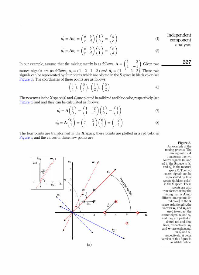
In our example, assume that the mixing matrix is as follows, A ¼�1 21 − 1
�. Given two
source signals are as follows, s1 ¼ ð 1 2 1 2 Þ and s2 ¼ ð 1 1 2 2 Þ. These twosignals can be represented by four points which are plotted in the S space in black color (seeFigure 5). The coordinates of these points are as follows:�
11
�;
�21
�;
�12
�;
�22
�(6)
The new axes in theXspace (s01 and s
02) are plotted in solid red and blue color, respectively (see
Figure 5) and and they can be calculated as follows:
s01 ¼ A
�10
�¼
�1 21 �1
��10
�¼
�11
�(7)
s02 ¼ A
�01
�¼
�1 21 �1
��01
�¼
�2
�1
�(8)
The four points are transformed in the X space; these points are plotted in a red color inFigure 5; and the values of these new points are
(a)
Figure 5.An example of the
mixing process. Themixing matrix A
transforms the twosource signals (s1 ands2) in the S space to (s
01
and s02) in the mixturespace X. The two
source signals can berepresented by four
points (in black color)in the S space. These
points are alsotransformed using themixing matrix A into
different four points (inred color) in the X
space. Additionally, thevectors w1 and w2 are
used to extract thesource signal s1 and s2,and they are plotted in
dotted red and bluelines, respectively. w1
and w2 are orthogonalon s
02 and s
01,
respectively. A colorversion of this figure is
available online.
Independentcomponent
analysis
227

�30
�;
�41
�;
�5
�1
�;
�60
�(9)
Assumed the second source s2 is silent/OFF; hence, the sensors record only the signal that is
generated from s1 (see Figure 6(a)). The mixed signals are laid along s01 ¼ ð a c ÞT and the
distribution of the projected samples onto s01 are depicted in Figure 6(a). Similarly, Figure 6(b)
shows the projection onto s02 ¼ ð b d ÞT when the first source is silent; this projection
represents the mixed data. It is worth mentioning that the new axes s01 and s
02 need not to be
orthogonal on the s1 and s2, respectively. Figure 5 is the combination of Figure 6(a) and (b)when both source signals are played together and the sensors measure the two signalssimultaneously.
A related point to consider is that the number of red points in Figure 6(a) which represent
the projected points onto s01 is three while the number of original points was four. This can be
interpreted mathematically by calculating the coordinates of the projected points onto s01. For
example, the projection of the first point ð 1 1 ÞT is calculated as follows,
s01ð 1 1 ÞT ¼
�11
�ð 1 1 ÞT ¼ 2. Similarly, the projection of the second, third, and fourth
points are 3; 3, and 4, respectively. Therefore, the second and third samples were projected
onto the same position onto s01. This is the reason why the number of projected points is three.
2.2 Unmixing signalsIn this section, the unmixing process for extracting source signals will be presented. Given amixingmatrixA, independent components can be estimated by inverting the linear system asin Eq. (2), but we know neither S nor A; hence, the problem is considerably more difficult.Assume that the matrix (A) is known; hence, source signals can be extracted. For simplicity,we assume that the number of sources and mixture signals are the same and hence theunmixing matrix is a square matrix.
Given two mixture signals x1 and x2. The aim is to extract source signals, and this can beachieved by searching for unmixing coefficients as follows:
y1 ¼ αx1 þ βx2
y2 ¼ γx1 þ δx2(10)
Figure 6.An example of themixing process. Themixing matrix Atransforms sourcesignals as follows: (a) s1is transformed from Sspace to s
01 ¼ ða; cÞT
(solid red line) whichis one of the axes ofthe mixture space X.The red stars representthe projection of thedata points onto s
01.
These red starsrepresent all samplesthat are generated fromthe first source s1. (b) s2is transformed from Sspace to s
02 ¼ ðb; dÞT
(solid blue line) whichis one of the axes of themixture space X. Theblue stars representthe projection of thedata points onto s
02.
These blue starsrepresent all samplesthat are generated fromthe second source s2.A color version of thisfigure is availableonline.
ACI17,2
228

where α; β; γ, and δ represent unmixing coefficients, which are used for transforming the
mixture signals into a set of independent signals as follow, X→Y : Y ¼ WTX, whereW∈Rn3p is the unmixing coefficients matrix as shown in Figure 7. Simply we can say thatthe first source signal, y1, can be extracted from the mixtures (x1 and x2) using two unmixingcoefficients (α and β). This pair of unmixing coefficients defines a point with coordinates
ðα; βÞ, where w1 ¼ ð α β ÞT is a weight vector (see Eq. (11)). Similarly, y2 can be extracted
using the two unmixing coefficients γ and δ which define the weight vector w2 ¼ ð γ δ ÞT(see Eq. (11))
y1 ¼ αx1 þ βx2 ¼ wT1 X
y2 ¼ γx1 þ δx2 ¼ wT2 X
(11)
W ¼ ðw1 w2 ÞT is the unmixing matrix and it represents the inverse of A. The unmixingprocess can be achieved by rotating the rows ofW. This rotation will continue till each row inW (w1 or w2) finds the orientation which is orthogonal on other transformed signals. Forexample, in our example, w1 is orthogonal on s
02 (see Figure 5). The source signals are then
extracted by projecting mixture signals onto that orientation.In practice, changing the length or orientation of weight vectors has a great influence on
the extracted signals (Y). This is the reason why the extracted signals may be not identical tooriginal source signals. The consequences of changing the length or orientation of the weightvectors are as follows:
� Length: The length of the weight vectorw1 is jw1j ¼ffiffiffiffiffiffiffiffiffiffiffiffiffiffiffiα2 þ β2
p, and assume that the
length of w1 is changed by a factor λ as follows, λjw1j ¼ λffiffiffiffiffiffiffiffiffiffiffiffiffiffiffiα2 þ β2
p¼ffiffiffiffiffiffiffiffiffiffiffiffiffiffiffiffiffiffiffiffiffiffiffiffiffiffiffi
ðλαÞ2 þ ðλβÞ2q
. The extracted signal or the best approximation of s1 is denoted by
y1 ¼ wT1 X and it is estimated as in Eq. (12). Hence, the extracted signal is a scaled
version of the source signal and the length of the weight vector affects only theamplitude of the extracted signal.
y1 ¼�λwT
1
�X ¼ ðλαÞx1 þ ðλβÞx2
¼ λðαx1 þ βx2Þ ¼ λs1(12)
� Orientation: As mentioned before, the source signals s1 and s2 in the S space are
transformed to s01 and s
02 (see Eqs. (4) and (5)), respectively, where s
01 and s
02 form the
mixture spaceX. The signal ðs1Þ is extracted only ifw1 is orthogonal to s02 and hence at
different orientations, different signals are extracted. This is because the inner product
Figure 7.An illustrative example
of the process ofextracting signals.Two source signals
(y1 and y2) areextracted from two
mixture signals (x1 andx2) using the unmixing
matrix W.
Independentcomponent
analysis
229
for any orthogonal vectors is zero as follows, y1 ¼ wT1 X ¼ wT
1 AS ¼ wT1 ð s
01 s
02Þ,
wherew1s02 ¼ 0 becausew1 is orthogonal to s
02, and the inner product ofw1 and s
01 is
as follows, wT1 s
01 ¼ jw1j
��s01
��cosθ ¼ jw1jjAs1jcosθ ¼ ks1, where θ is the angle
between w1 and s01 as shown in Figure 5, and k is a constant. The value of k
depends on the length of w1 and s01 and the angle θ. The extracted signal will be as
follows, y1 ¼ wT1 ð s
01 s
02Þ ¼ ðwT
1 s01 þwT
1 s02Þ ¼ ks1. The extracted signal (ks1) is a
scaled version from the source signal (s1), and ks1 is extracted from X by taking the
inner product of all mixture signals with w1 which is orthogonal to s02. Thus, it is
difficult to recover the amplitude of source signals.
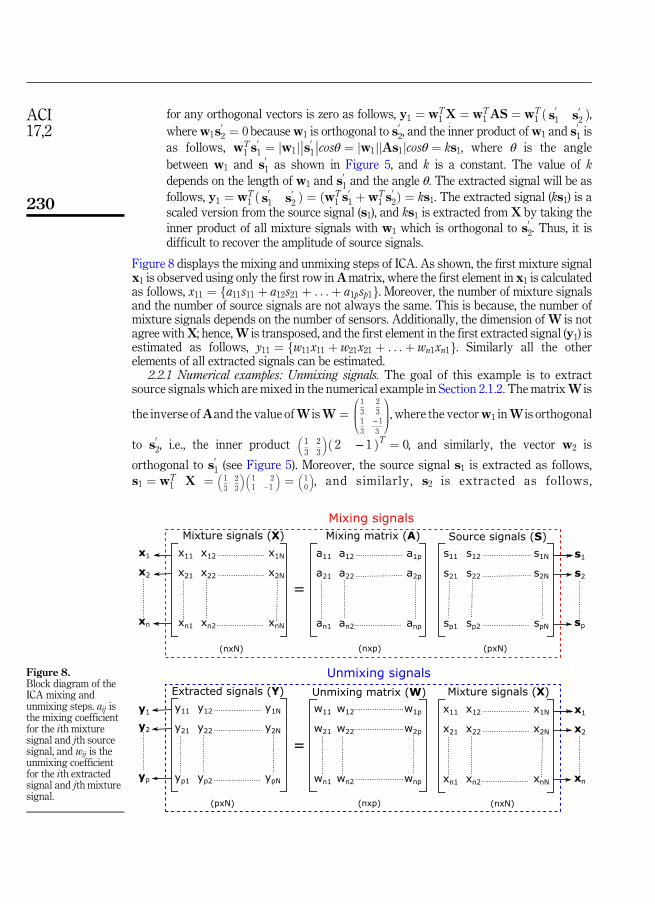
Figure 8 displays the mixing and unmixing steps of ICA. As shown, the first mixture signalx1 is observed using only the first row inAmatrix, where the first element in x1 is calculatedas follows, x11 ¼ fa11s11 þ a12s21 þ . . .þ a1psp1g. Moreover, the number of mixture signalsand the number of source signals are not always the same. This is because, the number ofmixture signals depends on the number of sensors. Additionally, the dimension of W is notagree withX; hence,W is transposed, and the first element in the first extracted signal (y1) isestimated as follows, y11 ¼ fw11x11 þ w21x21 þ . . .þ wn1xn1g. Similarly all the otherelements of all extracted signals can be estimated.
2.2.1 Numerical examples: Unmixing signals. The goal of this example is to extractsource signals which are mixed in the numerical example in Section 2.1.2. The matrixW is
the inverse ofAand the value ofW isW ¼0BB@
1
3
2
31
3
− 1
3
1CCA, where the vectorw1 inW is orthogonal
to s02, i.e., the inner product
�1
3
2
3
�ð 2 − 1 ÞT ¼ 0, and similarly, the vector w2 is
orthogonal to s01 (see Figure 5). Moreover, the source signal s1 is extracted as follows,
s1 ¼ wT1 X ¼ �
1
3
2
3
��1 21 – 1
� ¼ �10
�, and similarly, s2 is extracted as follows,
Figure 8.Block diagram of theICA mixing andunmixing steps. aij isthe mixing coefficientfor the ith mixturesignal and jth sourcesignal, and wij is theunmixing coefficientfor the ith extractedsignal and jth mixturesignal.
ACI17,2
230
s2 ¼ wT2 X ¼ �
1
3–1
3
��1 21 – 1
� ¼ �01
�. Hence, the original source signals are extracted
perfectly. This is because k≈ 1 and hence according to Eq. (12) the extracted signal isidentical to the source signal. As mentioned before, the value of k is calculated
as follows, k ¼ jw1j��s0
1
��cosθ, and the value of jw1j ¼ffiffiffiffiffiffiffiffiffiffiffiffiffiffiffiffiffiffiffiffiffið13Þ2 þ ð23Þ2
q¼
ffiffi5
p3 , and the value
of��s0
1
�� ¼ ffiffiffiffiffiffiffiffiffiffiffiffiffiffiffiffiffiffiffiffiffiffið1Þ2 þ ð1Þ2
q¼ ffiffiffi
2p
. The angle between s01 and the s1 axes is 458 because
s01 ¼ ð 1 1 ÞT; and similarly, the angle betweenw1 and s1 is cos
−1ð 1=3ffiffi5
p=3Þ ¼ cos−1ð 1ffiffi
5p Þ ≈ 638
(see Figure 5 top left corner). Therefore, θ≈ 638− 458≈ 188, and hence k ¼ffiffi59
q ffiffiffi2
pcos188≈ 1.
Hence, changing the orientation of w1 leads to a different extracted signal.
2.3 Ambiguities of ICAICA has some ambiguities such as:
� The order of independent components: In ICA, theweight vector ðwiÞ is initializedrandomly and then rotated to find one independent component. During the rotation, thevalue ofwi is updated iteratively. Thus,wi extracts source signals but not in a specificorder.
� The sign of independent components: Changing the sign of independentcomponents has not any influence on the ICA model. In other words, we can multiplythe weight vectors inW by −1without affecting the extracted signal. In our example,in Section 2.2.1, the value ofw1 was
�1
3
2
3
�. Multiplyingw1 by−1, i.e.,w1 ¼
�–1
3–2
3
�has
no influence becausew1 still in the same direction with the samemagnitude and hencethe value of k will not be changed, and the extracted signal s1 will be with the same
values but with a different sign, i.e., s1 ¼ wT1 X ¼ ð − 1 0 ÞT. As a result, the matrix
W in n-dimensional space has 2n local maxima, i.e., two local maxima for eachindependent component, corresponding to si and −si [21]. This problem isinsignificant in many applications [16,19].
3. ICA: Preprocessing phaseThis section explains the preprocessing steps of the ICA technique. This phase has two mainsteps: centering and whitening.
3.1 The centering stepThe goal of this step is to center the data by subtracting the mean from all signals. Given nmixture signals ðXÞ, the mean is μ and the centering step can be calculated as follows:
D ¼ X� μ ¼
0BB@
d1
d2
..
.
dn
1CCA ¼
0BB@
x1 � μx2 � μ
..
.
xn � μ
1CCA (13)
where D is the mixture signals after the centering step as in Figure 9A) and μ∈R13N is themean of all mixture signals. The mean vector can be added back to independent componentsafter applying ICA.
Independentcomponent
analysis
231
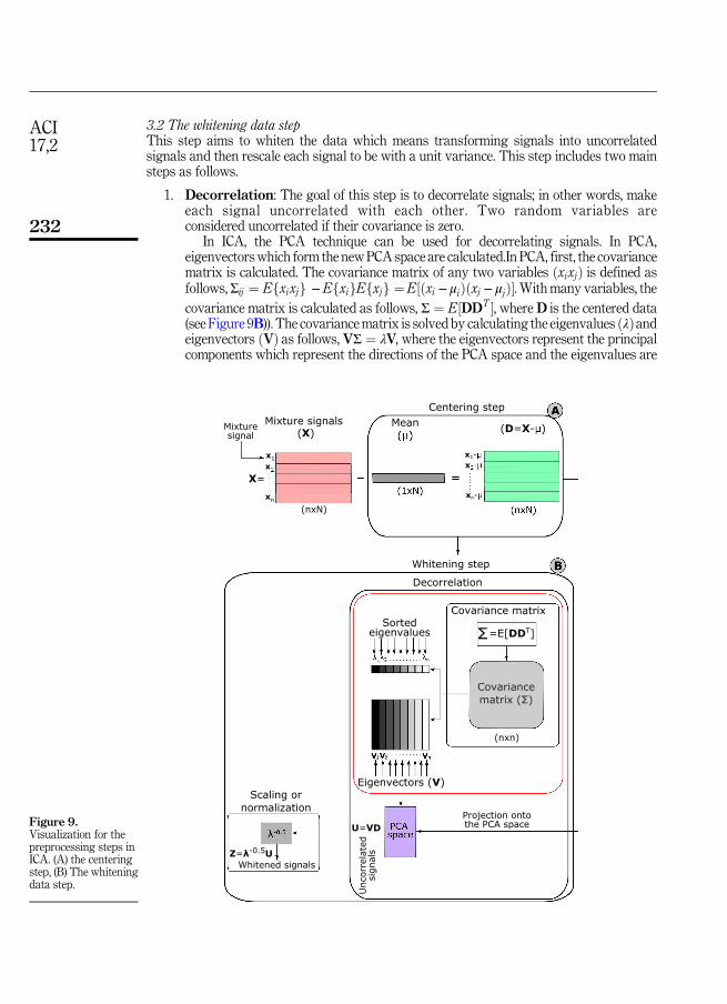
3.2 The whitening data stepThis step aims to whiten the data which means transforming signals into uncorrelatedsignals and then rescale each signal to be with a unit variance. This step includes two mainsteps as follows.
1. Decorrelation: The goal of this step is to decorrelate signals; in other words, makeeach signal uncorrelated with each other. Two random variables areconsidered uncorrelated if their covariance is zero.
In ICA, the PCA technique can be used for decorrelating signals. In PCA,eigenvectorswhich form the newPCA space are calculated.In PCA, first, the covariancematrix is calculated. The covariance matrix of any two variables ðxixjÞ is defined asfollows,Σij ¼ Efxixjg −EfxigEfxjg ¼E½ðxi − μiÞðxj − μjÞ�. Withmany variables, the
covariance matrix is calculated as follows, Σ ¼ E½DDT �, where D is the centered data(see Figure 9B)). The covariancematrix is solved by calculating the eigenvalues ðλÞandeigenvectors ðVÞ as follows, VΣ ¼ λV, where the eigenvectors represent the principalcomponents which represent the directions of the PCA space and the eigenvalues are
Figure 9.Visualization for thepreprocessing steps inICA. (A) the centeringstep, (B) The whiteningdata step.
ACI17,2
232

scalar values which represent the magnitude of the eigenvectors. The eigenvectorwhich has the maximum eigenvalue is the first principal component ðPC1Þ and it hasthe maximum variance [33]. For decorrelating mixture signals, they are projected ontothe calculated PCA space as follows, U ¼ VD.
2. Scaling: the goal here is to scale each decorrelated signal to be with a unitvariance. Hence, each vector in U has a unit length and is then rescaled to be
with a unit variance as follows, Z ¼ λ−12 U ¼ λ−
12VD, where Z is the whitened or
sphered data and λ−12 is calculated by simple component-wise operation as
follows, λ−12 ¼ fλ−1
2
1 ; λ−12
2 ; . . . ; λ−12
n g. After the scaling step, the data becomesrotationally symmetric like a sphere; therefore, the whitening step is also calledsphering [32].
3.3 Numerical exampleGiven eight mixture signalsX ¼ fx1; x2; . . . ;x8g, eachmixture signal is represented by onerow inX as in Eq. (14).6 The mean (μ) was then calculated and its value was μ ¼ 2:63 3:63 .
XT ¼�1:00 1:00 2:00 0:00 5:00 4:00 5:00 3:003:00 2:00 3:00 3:00 4:00 5:00 5:00 4:00
(14)
In the centering step, the data are centered by subtracting the mean from each signal and thevalue of Dwill be as follows:
DT ¼��1:63 �1:63 �0:63 �2:63 2:38 1:38 2:38 0:38�0:63 �1:63 �0:63 �0:63 0:38 1:38 1:38 0:38
(15)
The covariancematrix ðΣÞand its eigenvalues ðλÞand eigenvectors ðVÞare then calculated asfollows:
Σ ¼�3:70 1:701:70 1:13
; λ ¼
�0:28 0:000:00 4:54
; andV ¼
�0:45 �0:90�0:90 �0:45
(16)
From Eq. (16) it can be remarked that the two eigenvectors are orthogonal as shown inFigure 10, i.e., vT1 v2 ¼ ½0:45− 0:9�− 0:90− 0:45T ¼ 0, where v1 and v2 represent the firstand second eigenvectors, respectively. Moreover, the value of the second eigenvalueðλ2Þ was more than the first one ðλ1Þ, and λ2 represents 4:54
0:28þ4:54≈ 94:19% of the totaleigenvalues; thus, v2 and v1 represent the first and second principal components of thePCA space, respectively, and v2 points to the direction of the maximum variance (seeFigure 10).
The two signals are decorrelated by projecting the centered data onto the PCA space asfollows, U ¼ VD. The values of U is
UT ¼��0:16 0:73 0:28 �0:61 0:72 �0:62 �0:18 �0:171:73 2:18 0:84 2:63 �2:29 �1:84 �2:74 �0:50
(17)
Independentcomponent
analysis
233

The matrix U is already centered; thus, the covariance matrix for U is given by
E�UUT
� ¼ �0:28 00 4:54
(18)
From Eq. (18) it is remarked that the twomixture signals are decorrelated by projecting themonto the PCA space. Thus, the covariance matrix is diagonal and the off-diagonal elementswhich represent the covariance between twomixture signals are zeros. Figure 10 displays thecontour of the two mixtures is ellipsoid centered at the mean. The projection of mixturesignals onto the PCA space rotates the ellipse so that the principal components are alignedwith the x1 and x2 axes. After the decorrelation step, the signals are then rescaled to be with aunit variance (see Figure 10). The whitening can be calculated as follows,Z ¼ λ−
12VD, and the
values of the mixture signals after the scaling step are
ZT ¼��0:31 1:38 0:53 �1:15 1:36 �1:17 �0:33 �0:320:81 1:02 0:39 1:23 �1:08 �0:87 �1:29 �0:24
(19)
The covariance matrix for the whitened data is E½ZZT � ¼ E½ðλ−0:5VDÞðλ−0:5VDÞT � ¼E½ðλ−0:5VDÞðDTVTλ−0:5Þ�. λ is diagonal; thus, λ ¼ λT, and ½DDT � is the covariance matrix
ðΣÞwhich is equal to VTλV. Hence, E½ZZT � ¼ E½λ−0:5VVTλVVTλ−0:5� ¼ I, where VVT ¼ IbecauseV is orthonormal.7 This means that the covariance matrix of the whitened data is theidentity matrix (see Eq. (20)) which means that the data are decorrelated and have unitvariance.
E�ZZT
� ¼ �1:00 00 1:00
(20)
Figure 11 displays the scatter plot for twomixtures, where eachmixture signal is representedby 500-time steps. As shown in Figure 11(a), the scatter of the original mixtures forms an
Figure 10.Visualization for ourwhitening example. Inthe left panel, themixture signals areplotted in red stars.This panel also showsthe principalcomponents (PC1 andPC2). In the top rightpanel, the data in a bluecolor represent theprojected data onto thePCA space. The dataare then normalized tobe with a unit variance(the bottom rightpanel). In this panel, thedata in a green colorrepresent the whiteneddata. A color version ofthis figure is availableonline.
ACI17,2
234

)b(
)a(
(c)
Figure 11.Visualization for
mixture signals duringthe whitening step. (a)
scatter plot for twomixture signals x1 andx2, (b) the projection ofmixture signals ontothe PCA space, i.e.,decorrelation, (c)
mixture signals afterthe whitening step arescaled to have a unit
variance.
Independentcomponent
analysis
235

ellipse centered at the origin. Projecting the mixture signals onto the PCA space rotates theprincipal components to be alignedwith the x1 and x2 axes and hence the ellipse is also rotatedas shown in Figure 11(b). After the whitening step, the contour of the mixture signals forms acircle. This is because the signals have unit variance.
4. Principles of ICA estimationIn ICA, the goal is to find the unmixing matrix ðWÞ and then projecting the whitened dataonto that matrix for extracting independent signals. This matrix can be estimated usingthree main approaches of independence, which result in slightly different unmixingmatrices. The first is based on the non-Gaussianity. This can bemeasured by somemeasuressuch as negentropy and kurtosis, and the goal of this approach is to find independentcomponents which maximize the non-Gaussianity [25,30]. In the second approach, the ICAgoal can be obtained byminimizing themutual information [22,14]. Independent componentscan be also estimated by using maximum likelihood (ML) estimation [28]. All approachessimply search for a rotation or unmixing matrixW. Projecting the whitened data onto thatrotation matrix extracts independent signals. The preprocessing steps are calculated fromthe data, but the rotation matrix is approximated numerically through an optimizationprocedure. Searching for the optimal solution is difficult due to the local minima exists in theobjective function. In this section, different approaches are introduced for extractingindependent components.
4.1 Measures of non-GaussianitySearching for independent components can be achieved by maximizing the non-Gaussianityof extracted signals [23]. Twomeasures are used for measuring the non-Gaussianity, namely,Kurtosis and negative entropy.
4.1.1 Kurtosis. Kurtosis can be used as a measure of non-Gaussianity, and the extractedsignal can be obtained by finding the unmixing vector which maximizes the kurtosis of theextracted signal [4]. In other words, the source signals can be extracted by finding theorientation of the weight vectors which maximize the kurtosis.
Kurtosis is simple to calculate; however, it is sensitive for outliers. Thus, it is not robustenough for measuring the non-Gaussianity [21]. The Kurtosis (K) of any probability densityfunction (pdf) is defined as follow,
KðxÞ ¼ Ex4�� 3
E½x2��2 (21)
where the normalized kurtosis ðbKÞ is the ratio between the fourth and second centralmoments, and it is given by
bKðxÞ ¼ E½x4�E½x2�2 � 3 ¼
1N
PN
i¼1ðxi � μÞ41N
PN
i¼1ðxi � μÞ2� 2
� 3 (22)
For whitened data ðZÞ,E½Z2� ¼ 1becauseZwith a unit variance. Therefore, the kurtosis willbe
KðZÞ ¼ bKðZÞ ¼ EZ4
�� 3 (23)
As reported in [20], the fourth moment for Gaussian signals is 3ðE½Z2�Þ2 and
hence bKðxÞ ¼ E½Z4�− 3 ¼ E½3ðE½Z2�Þ2�− 3 ¼ E½3ð1Þ2�− 3 ¼ 0, where E½Z2� ¼ 1. As aconsequence, Gaussian pdfs have zero kurtosis.
ACI17,2
236

Kurtosis has an additivity property as follows:
Kðx1 þ x2Þ ¼ Kðx1Þ þ Kðx2Þ; (24)
and for any scalar parameter α,
Kðαx1Þ ¼ α4Kðx1Þ (25)
where α is a scalar.These properties can be used for interpreting one of the ambiguities of ICA that are
mentioned in Section 2.3, which is the sign of independent components. Given two source
signals s1 and s2, and the matrix Q ¼ ATW ¼ A−1W. Hence,
Y ¼ WTX ¼ WTAS ¼ QS ¼ q1s1 þ q2s2 (26)
Using the kurtosis properties in Eqs. (24) and (25), we have
KðYÞ ¼ Kðq1s1Þ þ Kðq2s2Þ ¼ q41Kðs1Þ þ q4
2Kðs2Þ (27)
Assume that s1; s2, and Y have a unit variance. This implies that E½Y2� ¼q21E½s1� þ q2
2E½s2� ¼ q21 þ q2
2 ¼ 1. Geometrically, this means that Q is constrained to a unitcircle in the two-dimensional space. The aim of ICA is to maximize the kurtosisðKðYÞ ¼ q4
1K ðs1Þ þ q42K ðs2ÞÞ on the unit circle. The optimal solutions, i.e., maxima, are the
points when one ofQ is zero and the other is nonzero; this is due to the unit circle constraint, andthe nonzero element must be 1 or�1 [11]. These optimal solutions are the ones which are used to
extract ±si. Generally, Q ¼ ATW ¼ I means that each vector in the matrix Q extracts onlyone source signal.
The ICs can be obtained by finding the ICs which maximizes kurtosis of extracted signals
Y ¼ WTZ. The kurtosis of Y is then calculated as in Eq. (23), where the term ðE½y2i �Þ
2in
Eq. (22) is equal one because W andZ have a unit length. W has a unit length because it isscaled to be with a unit length, and Z is the whitened data, so, it has a unit length. Thus, thekurtosis can be expressed as:
KðYÞ ¼ Eh�WTZ
�4i� 3 (28)
The gradient of the kurtosis ofY is given by, vKðWTZÞvW
¼ cE½ZðWTZÞ3�, where c is a constant,which we set to unity for convenience. The weight vector is updated in each iteration as
follows,wnew ¼ wold þ ηE½ZðwToldZÞ
3�, where η is the step size for the gradient ascent. Sincewe are optimizing the kurtosis on the unit circle kwk ¼ 1, the gradient method must becomplemented by projecting w onto the unit circle after every step. This can be done bynormalizing the weight vectors wnew through dividing it by its norm as follows,wnew ¼ wnew=kwnewk. The value of wnew is updated in each iteration.
4.1.2Negative entropy.Negative entropy is termed negentropy, and it is defined as follows,JðyÞ ¼ HðyGaussianÞ−HðyÞ, where HðyGaussianÞ is the entropy of a Gaussian random variablewhose covariance matrix is equal to the covariance matrix of y. The entropy of a randomvariable Q which has N possible outcomes is
HðQÞ ¼ −Elog pqðqÞ
� ¼ –1
N
XNt
log pq�qt�
(29)
where pqðqtÞ is the probability of the event qt; t ¼ 1; 2; . . . ; N.
Independentcomponent
analysis
237

The negentropy is zero when all variables are Gaussian, i.e., HðyGaussianÞ ¼ HðyÞ.Negentropy is always nonnegative because the entropy of Gaussian variable is themaximumamong all other random variables with the same variance. Moreover, it is invariant forinvertible linear transformation and it is scale-invariant [21]. However, calculating theentropy from a finite data is computationally difficult. Hence, different approximations havebeen introduced for calculating the negentropy [21]. For example,
JðyÞ≈ 1
12Ey3�2 þ 1
48KðyÞ2 (30)
where y is assumed to be with zero mean. This approximation suffers from the sensitivity ofkurtosis; therefore, Hyvarinen proposed another approximation based on the maximumentropy principle as follows [23]:
JðyÞ≈Xp
i¼1
kiðE½GiðyÞ� � E½GiðvÞ�Þ2; (31)
where ki are some positive constants, v indicates a Gaussian variable with zero mean and unitvariance, Gi represent some quadratic functions [23,20]. The function G has different choicessuch as
G1ðyÞ ¼ 1
a1log cosh a1y andG2ðyÞ ¼ −exp
�−y2
�2�
(32)
where 1≤ a1 ≤ 2. These two functions are widely used, and these approximations give a verygood compromise between the kurtosis and negentropy propertieswhich are the two classicalnon-Gaussianity measures.
4.2 Minimization of mutual informationMinimizing mutual information between independent components is one of the well-known
approaches for ICA estimation. In ICA, maximizing the entropy of Y ¼ WTX can be
achieved by spreading out the points inY as much as possible. Signals bY can be obtained by
transforming Y by g as follows, bY ¼ gðYÞ, where g is assumed to be the cumulative density
function cdf of source signals. Hence, bY have a uniform joint distribution.
The pdf of the linear transformation Y ¼ WTX is, pY ðYÞ ¼ pX ðXÞ=jWj, where jWjrepresents jvY=vXj. Similarly, pbY ðbYÞ ¼ pY ðYÞ=
���� dbYdY���� ¼ pY ðYÞ
pSðYÞ, where���� dbYdY
���� is equal to g0 ðyÞ
which represents the pdf for source signals (pS).This can be substituted in Eq. (29) and the entropy will be
HðbYÞ ¼ –1
N
XNt¼1
log pbYðbYtÞ ¼ –1
N
XNt
logpY ðYÞpSðYÞ ¼ −
1
N
XNt¼1
logpX ðxtÞ
jWjpSðytÞ
¼ 1
N
XNt¼1
log pSðytÞ þ log jWj � 1
N
XNt¼1
log pX ðxtÞ (33)
In Eq. (33), increasing the matching between the extracted and source signals, the ratio pY ðYÞpSðYÞ
will be one. As a consequence, the pbY ðbYÞ ¼ pY ðYÞpS ðYÞ becomes uniform which maximizes the
entropy of pbY ðbYÞ. Moreover, the term −1N
PNt¼1log pX ðXtÞ represents the entropy ofX; hence,
Eq. (33) is given by
ACI17,2
238

HðbYÞ ¼ 1
N
XNt¼1
log pSðytÞ þ log jWj þ HðXÞ (34)
Hence, from Eq. (34),HðYÞ ¼ HðXÞ þ log jWj. This means that in the linear transformation
Y ¼ WTX, the entropy is changed (increased or decreased) by logjWj. As mentioned before,
the entropy HðXÞ is not affected byW andWmaximizes only the entropy HðbYÞ and henceHðXÞ is removed from Eq. (34), and final form of the entropy with M marginal pdfs is
HðbYÞ ¼ 1
N
XNt¼1
XMi¼1
log pS�yit
�þ log jWj (35)
Mutual information measures the independence between random variables. Thus,independent components can be obtained by minimizing the mutual information betweendifferent components [6]. Given two random variables x and y, the mutual information isdenoted by I, and it is given by
Iðx; yÞ ¼Xx;y
pðx; yÞlog pðx; yÞpðxÞpðyÞ
¼ HðxÞ � HðxjyÞ ¼ HðyÞ � HðyjxÞ¼ HðxÞ þ HðyÞ � Hðx; yÞ¼ Hðx; yÞ � HðxjyÞ � HðyjxÞ
(36)
where HðxÞ and HðyÞ represent the marginal entropies, HðxjyÞ and HðyjxÞ are conditionalentropies, and Hðx; yÞ is the joint entropy of x and y. The value of I is zero if and only if thevariables are independent; otherwise, I is non-negative. Mutual information between mrandom variables ðyi; i ¼ 1; 2; . . . ; mÞ is given by
Iðy1; y2; . . . ; ymÞ ¼Xmi¼1
HðyiÞ � HðyÞ (37)
In ICA, where Y ¼ WTX and HðYÞ ¼ HðXÞ þ log jWj, Eq. (37) can be written as
Iðy1;y2; . . . ;ymÞ ¼Xmi¼1
HðyiÞ � HðYÞ
¼Xmi¼1
HðyiÞ � HðXÞ � logjdetWj(38)
where detW is a notation for a determine of the matrix W. When Y is whitened; thus,
E½YYT � ¼ WE½XXT �WT ¼ I0detðWE½XXT �WTÞ ¼ ðdetWÞ ðdetE½XXT �ÞðdetWTÞ0det ðWE½XXT �WTÞ ¼ detI ¼ 1. As a consequence, detW is a constant, and the definition ofmutual information is
Iðy1; y2; . . . ; ymÞ ¼ C �Xi
JðyiÞ (39)
where C is a constant.From Eq. (39), it is clear that maximizing negentropy is related to minimizing mutual
information and they differ only by a sign and a constant C. Moreover, non-Gaussianitymeasures enable the deflationary (one-by-one) estimation of the ICswhich is not possible withmutual information or likelihood approaches.8 Further, with the non-Gaussianity approach,
Independentcomponent
analysis
239

all signals are enforced to be uncorrelated, while this constraint is not necessary usingmutualinformation approach.
4.3 Maximum Likelihood (ML)Maximum likelihood (ML) estimation method is used for estimating parameters of statisticalmodels given a set of observations. In ICA, this method is used for estimating the unmixingmatrix ðWÞwhich provides the best fit for extracted signals Y.
The likelihood is formulated in the noise-free ICA model as follows, X ¼ AS, and this
model can be estimated using ML method [6]. Hence, pX ðXÞ ¼ pS ðSÞjdetAj ¼ jdetWjpSðSÞ. For
independent source signals, ði:e: pSðSÞ ¼ p1ðs1Þp2ðs2Þ . . . ppðspÞ ¼Q
ipiðsiÞÞ, pX ðXÞ isgiven by
pxðXÞ ¼ jdetWjYi
piðsiÞ ¼ jdetWjYi
pi�wT
i X�
(40)
Given T observations of X, the log-likelihood of Wwhich is denoted by LðWÞ is given by
LðWÞ ¼YTt
Ypi
jdetWjpi�wT
i xðtÞ�
(41)
Practically, the likelihood is usually simplified using the logarithm, this is calledlog-likelihood, which makes Eq. (41) more simpler as follows:
logLðWÞ ¼Xp
i¼1
log pi�wT
i xðtÞ�þ TlogjdetWj (42)
Themean of any randomvariable x can be calculated asE½x� ¼ 1T
PTi¼1xt0
PTi¼1xt ¼ TE½x�.
Hence, Eq. (42) can be simplified to
1
TlogLðWÞ ¼ E
Xp
i¼1
log pi�wT
i X�þ logjdetWj (43)
The first term EP
i¼1log piðwTi XÞ ¼ −
Pi¼1HðwT
i XÞ; therefore, the likelihood and mutualinformation are approximately equal, and they differ only by a sign and an additive constant.It is worth mentioning that maximum likelihood estimation will give wrong results if theinformation of ICs are not correct; but, with the non-Gaussianity approach, we need not forany prior information [23].
5. ICA algorithmsIn this section, different ICA algorithms are introduced.
5.1 Projection pursuitProjection pursuit (PP) is a statistical technique for finding possible projections of multi-dimensional data [13]. In the basic one-dimensional projection pursuit, the aim is to find thedirectionswhere the projections of the data onto these directions have distributionswhich aredeviated fromGaussian distribution, and this exactly is the same goal of ICA [13]. Hence, ICAis considered as a variant of projection pursuit.
In PP, one source signal is extracted from each projection, which is different than ICAalgorithms that extract p signals simultaneously from nmixtures. Simply, in PP, after findingthe first projectionwhichmaximizes the non-Gaussianity, the same process is repeated to find
ACI17,2
240

new projections for extracting next source signal(s) from the reduced set of mixture signals,and this sequential process is called deflation [17].
Given nmixture signals which represent the axes of the n-dimensional space ðXÞ. The nthsource signal can be extracted using the vectorwnwhich is orthogonal to the other n− 1axes.These mixture signals in the n-dimensional space are projected onto the ðn− 1Þ-dimensionalspace which has n− 1 transformed axes. For example, assume n ¼ 3, and the third sourcesignal can be extracted by findingw3 which is orthogonal to the plane that is defined by the
other two transformed axes s01 and s
02; this plane is denoted by p
01;2. Hence, the data points in
three-dimensional space are projected onto the plane p01;2 which is a two-dimensional space.
This process is continued until all source signals are extracted [20,32].Given three source signals each source signal has 10000 time-steps as shown in Figure 12.
These signals represent sound signals. These sound signals were collected from Matlab,where the first signal is called Chrip, the second signal is called gong, and the third is calledtrain. Figure 12 (d, e, and f) shows the histogram for each signal. As shown, the histogramsare non-Gaussian. These three signals were mixed, and the mixing matrix was as follows:
A ¼0@ 1:5 0:7 0:2
0:6 0:2 0:90:1 1 0:6
1A (44)
Figure 13 shows the mixed signals and the histogram for these mixture signals. As shown inthe figure, the mixture signals follow all the properties that were mentioned in Section 2.1.1,where (1) source signals are more independent than mixture signals, (2) the histograms ofmixture signals in Figure 13 are much more Gaussian than the histogram of source signals inFigure 12mixtures signals (see Figure 13 aremore complex than source signals (see Figure 12)).
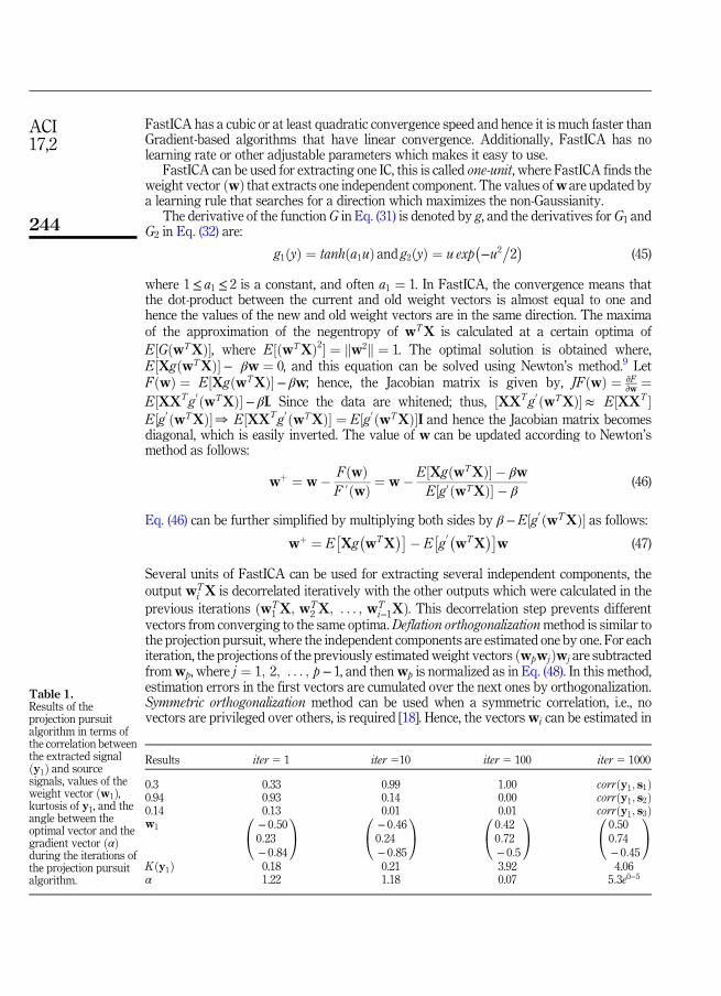
In the projection pursuit algorithm, mixture signals are first whitened, and then the valuesof the first weight vector ðw1Þ are initialized randomly. The value of w1 is listed in Table 1.This weight vector is then normalized, and it will be used for extracting one source signalðy1Þ. The kurtosis for the extracted signal is then calculated and the weight vector is updatedtomaximize the kurtosis iteratively. Table 1 shows the kurtosis of the extracted signal duringsome iterations of the projection pursuit algorithm. It is remarked that the kurtosis increasesduring the iterations as shown in Figure 14(a). Moreover, in this example, the correlationbetween the extracted signal ðy1Þ and all source signals (s1; s2, and s3) were calculated. Thismay help to understand that how the extracted signal is correlatedwith one source signal andnot correlated with the other signals. From the table, it can be remarked that the correlationbetween y1 and source signals are changed iteratively, and the correlation between y1 and s1was 1 at the end of iterations.
Figure 15 shows the histogram of the extracted signal during the iteration. As shown inFigure 15(a), the extracted signal is Gaussian; hence, its kurtosis value which represents themeasure of non-Gaussianity in the projection pursuit algorithm is small (0.18). The kurtosisvalue of the extracted signal increased to 0.21, 3.92, and 4.06 after the 10th, 100th, and 1000thiterations, respectively. This reflects that the non-Gaussianity of y1 increased during theiterations of the projection pursuit algorithm. Additionally, Figure 14(b) shows the anglebetween the optimal vector and the gradient vector ðαÞ. As shown, the value of the angle isdramatically decreased and it reached zero which means that both the optimal and gradientvectors have the same direction.
5.2 FastICAFastICA algorithm extracts independent components bymaximizing the non-Gaussianity bymaximizing the negentropy for the extracted signals using a fixed-point iteration scheme [18].
Independentcomponent
analysis
241

)c()b(
)a(
)e()d(
(f)
Figure 12.Three source signals inour example (a, b, and c)and their histograms(d, e, and f).
ACI17,2
242

)c()b(
)a(
)e()d(
(f)
Figure 13.Three mixture signalsin our example (a, b,
and c) and theirhistograms (d, e, and f).
Independentcomponent
analysis
243
FastICA has a cubic or at least quadratic convergence speed and hence it is much faster thanGradient-based algorithms that have linear convergence. Additionally, FastICA has nolearning rate or other adjustable parameters which makes it easy to use.
FastICA can be used for extracting one IC, this is called one-unit, where FastICA finds theweight vector ðwÞ that extracts one independent component. The values ofw are updated bya learning rule that searches for a direction which maximizes the non-Gaussianity.
The derivative of the function G in Eq. (31) is denoted by g, and the derivatives for G1 andG2 in Eq. (32) are:
g1ðyÞ ¼ tanhða1uÞ and g2ðyÞ ¼ u exp�−u2
�2�
(45)
where 1≤ a1 ≤ 2 is a constant, and often a1 ¼ 1. In FastICA, the convergence means thatthe dot-product between the current and old weight vectors is almost equal to one andhence the values of the new and old weight vectors are in the same direction. The maximaof the approximation of the negentropy of wTX is calculated at a certain optima of
E½GðwTXÞ�, where E½ðwTXÞ2� ¼ kw2k ¼ 1. The optimal solution is obtained where,E½XgðwTXÞ�− βw ¼ 0, and this equation can be solved using Newton’s method.9 LetFðwÞ ¼ E½XgðwTXÞ�− βw; hence, the Jacobian matrix is given by, JFðwÞ ¼ vF
vw¼
E½XXTg0 ðwTXÞ�− βI. Since the data are whitened; thus, ½XXTg
0 ðwTXÞ�≈ E½XXT �E½g 0 ðwTXÞ�0 E½XXTg
0 ðwTXÞ� ¼ E½g 0 ðwTXÞ�I and hence the Jacobian matrix becomesdiagonal, which is easily inverted. The value of w can be updated according to Newton’smethod as follows:
wþ ¼ w� FðwÞF 0 ðwÞ ¼ w� E½XgðwTXÞ� � βw
E½g 0 ðwTXÞ� � β(46)
Eq. (46) can be further simplified by multiplying both sides by β−E½g 0 ðwTXÞ� as follows:wþ ¼ E
Xg
�wTX
��� Eg
0�wTX
��w (47)
Several units of FastICA can be used for extracting several independent components, theoutput wT
i X is decorrelated iteratively with the other outputs which were calculated in the
previous iterations ðwT1 X; wT
2 X; . . . ; wTi−1XÞ. This decorrelation step prevents different
vectors from converging to the same optima.Deflation orthogonalizationmethod is similar tothe projection pursuit, where the independent components are estimated one by one. For eachiteration, the projections of the previously estimated weight vectors ðwpwjÞwj are subtractedfromwp, where j ¼ 1; 2; . . . ; p− 1, and thenwp is normalized as in Eq. (48). In this method,estimation errors in the first vectors are cumulated over the next ones by orthogonalization.Symmetric orthogonalization method can be used when a symmetric correlation, i.e., novectors are privileged over others, is required [18]. Hence, the vectorswi can be estimated in
Results iter 5 1 iter 510 iter 5 100 iter 5 1000
0.3 0.33 0.99 1.00 corrðy1; s1Þ0.94 0.93 0.14 0.00 corrðy1; s2Þ0.14 0.13 0.01 0.01 corrðy1; s3Þw1
0@ − 0:50
0:23− 0:84
1A
0@ − 0:46
0:24− 0:85
1A
0@ 0:42
0:72− 0:5
1A
0@ 0:50
0:74− 0:45
1A
Kðy1Þ 0.18 0.21 3.92 4.06α 1.22 1.18 0.07 5:3e0−5
Table 1.Results of theprojection pursuitalgorithm in terms ofthe correlation betweenthe extracted signalðy1Þ and sourcesignals, values of theweight vector ðw1Þ,kurtosis of y1, and theangle between theoptimal vector and thegradient vector ðαÞduring the iterations ofthe projection pursuitalgorithm.
ACI17,2
244

parallel which enables parallel computation. This method calculates all wi vectors using one-unit algorithm in parallel, and then the orthogonalization step is applied for all vectors using
symmetric method as follows, W ¼ ðWWTÞ−12W, where ðWWTÞ−1
2 is calculated from the
eigenvalue decomposition as follows, VðWWTÞ ¼ λV; thus, ðWWTÞ−12 ¼ VTλ−
12V.
1:wp ¼ wp �Xp
j¼1
wTp wjwj
2:wp ¼ wpffiffiffiffiffiffiffiffiffiffiffiffiwT
p wp
q (48)
6. ApplicationsICA has been used in many applications for extracting source signals from a set of mixedsignals. These applications include:
� Biomedical applications: ICA was used for removing artifacts which mixed withdifferent biomedical signals such as Electroencephalogram (EEG), functional magneticresonance imaging (fMRI), andMagnetoencephalography (MEG) signals [5]. Also, ICAwas used for removing the electrocardiogram (ECG) interference from EEG signals, orfor differentiating between the brain signals and the other signals that are generatedfrom different activities as in [29].
� Audio signal processing: ICA has been widely used in audio signals for removingnoise [36]. Additionally, ICAwas used as a feature extraction method to design robustautomatic speech recognition models [8].
� Biometrics: ICA is for extracting discriminative features in different biometrics suchas face recognition [10], ear recognition [35], and finger print [27].
� Image processing: ICA is used in image segmentation to extract different layersfrom the original image [12]. Moreover, ICA is widely used for noise removing fromraw images which represent the original signals [24].
7. Challenges of ICAICA is used for estimating the unknown matrix W ¼ A−1. When the number of sources (p)and the number of mixture signals (n) are equal, the matrixA is invertible. When the number
)b()a(
Figure 14.Results of the
projection pursuitalgorithm. (a) Kurtosisof the extracted signal
(y1) during someiterations of the
projection pursuitalgorithm, (b) the angle
between the optimalvector and gradient
vector ðαÞ during someiterations of the
projection pursuitalgorithm.
Independentcomponent
analysis
245

(a)
(b)
(c)
(d)
Figure 15.Histogram of theextracted signal ðy1Þ.(a) after the firstiteration, (b) after thetenth iteration, (c) afterthe 100th iteration, and(d) after the 1000thiteration.
ACI17,2
246

of mixtures is less than the number of source signals ðn < pÞ this is called the over-completeproblem; thus, A is not square and not invertible [26]. This representation sometimes isadvantageous as it uses as few “basis” elements as possible; this is called sparse coding. Onthe other hand, when n > pmeans that the number of mixtures is higher than the number ofsource signals and this is called the Under-complete problem. This problem can be solved bydeleting some mixtures using dimensionality reduction techniques such as PCA to decreasethe number of mixtures [1].
8. ConclusionsICA is a widely-used statistical technique which is used for estimating independentcomponents (ICs) through maximizing the non-Gaussianity of ICs, maximizing the likelihoodof ICs, or minimizing mutual information between ICs. These approaches are approximatelyequivalent; however, each approach has its own limitations.
This paper followed the approach of not only explaining the steps for estimating ICs, butalso presenting illustrative visualizations of the ICA steps to make it easy to understand.Moreover, a number of numerical examples are introduced and graphically illustrated toexplain (1) how signals are mixed to formmixture signals, (2) how to estimate source signals,and (3) the preprocessing steps of ICA. Different ICA algorithms are introduced with detailedexplanations. Moreover, ICA common challenges and applications are briefly highlighted.
Notes1 In this paper, original signals, source signals, or independent components (ICs) are the same.2 In this paper, source and mixture signals are represented as random variables instead of time series ortime signals, i.e., the time index is dropped.
3 Two signals s1 and s2 are independent if the amplitude of s1 is independent of the amplitude of s2.4 In this paper, all bold lowercase letters denote vectors and bold uppercase letters indicate matrices.5 In all numerical examples, the numbers are rounded up to the nearest hundredths (two numbers afterthe decimal point).
6 Due to the paper size, Eq. (14) indicates XT instead of X; hence, each column represents one signal/sample. Similarly, D in Eq. (15), U in Eq. (17), and Z in Eq. (19).
7 Two vectors x and y are orthonormal if they are orthogonal, i.e., the dot product x:y ¼ 0, and they areunit vectors, i.e., ðxÞ ¼ ðyÞ ¼ 1.
8 Maximum Likelihood approach will be introduced in the next section.9 Assume f ðxÞ ¼ 0, using Newton’s method, the solution is calculated as follows, xiþ1 ¼ xi −
f ðxÞf0 ðxÞ.
References
[1] S.-I. Amari, Natural gradient learning for over-and under-complete bases in ICA, Neural Comput.11 (8) (1999) 1875–1883.
[2] A. Asaei, H. Bourlard, M.J. Taghizadeh, V. Cevher, Computational methods for underdeterminedconvolutive speech localization and separation via model-based sparse component analysis,Speech Commun. 76 (2016) 201–217.
[3] R. Aziz, C. Verma, N. Srivastava, A fuzzy based feature selection from independent componentsubspace for machine learning classification of microarray data, Genomics data 8 (2016) 4–15.
[4] E. Bingham, A. Hyv€arinen, A fast fixed-point algorithm for independent component analysis ofcomplex valued signals, Int. J. Neural Syst. 10 (01) (2000) 1–8.
Independentcomponent
analysis
247
[5] V.D. Calhoun, J. Liu, T. Adal, A review of group ICA for FMRA data and ICA for joint inference ofimaging, genetic, and ERP data, Neuroimage 45 (1) (2009) S163–S172.
[6] J.-F. Cardoso, Infomax and maximum likelihood for blind source separation, IEEE Sig. Process.Lett. 4 (4) (1997) 112–114.
[7] R. Chai, G.R. Naik, T.N. Nguyen, S.H. Ling, Y. Tran, A. Craig, H.T. Nguyen, Driver fatigueclassification with independent component by entropy rate bound minimization analysis in aneeg-based system, IEEE J. Biomed. Health Inf. 21 (3) (2017) 715–724.
[8] J.-W. Cho, H.-M. Park, Independent vector analysis followed by hmm-based feature enhancementfor robust speech recognition, Sig. Process. 120 (2016) 200–208.
[9] P. Comon, Independent component analysis, a new concept?, Sig. Process. 36 (3) (1994) 287–314.
[10] I. Dagher, R. Nachar, Face recognition using ipca-ica algorithm, IEEE Trans. Pattern Anal.Machine Intell. 28 (6) (2006) 996–1000.
[11] N. Delfosse, P. Loubaton, Adaptive blind separation of independent sources: a deflation approach,Sig. Process. 45 (1) (1995) 59–83.
[12] S. Derrode, G. Mercier, W. Pieczynski, Unsupervised multicomponent image segmentationcombining a vectorial hmc model and ica, in: Proceedings of International Conference on ImageProcessing (ICIP), Vol. 2, IEEE, 2003, pp. II–407.
[13] J.H. Friedman, J.W. Tukey, A projection pursuit algorithm for exploratory data analysis, IEEETrans. Comput. 100 (9) (1974) 881–890.
[14] S.S. Haykin, S.S. Haykin, S.S. Haykin, S.S. Haykin, Neural Netw. Learn. Machines, Vol. 3, PearsonUpper Saddle River, NJ, USA, 2009.
[15] J. H�erault, C. Jutten, B. Ans, D�etection de grandeurs primitives dans un message composite parune architecture de calcul neuromim�etique en apprentissage non supervis�e. In: 10 Colloque sur letraitement du signal et des images, FRA, 1985.GRETSI, Groupe d’Etudes du Traitement duSignal et des Images 1985.
[16] A. Hyv€arinen, Independent component analysis in the presence of gaussian noise by maximizingjoint likelihood, Neurocomputing 22 (1) (1998) 49–67.
[17] A. Hyv€arinen, New approximations of differential entropy for independent component analysisand projection pursuit. In: Advances in neural information processing systems. (1998b)pp. 273–279.
[18] A. Hyvarinen, Fast and robust fixed-point algorithms for independent component analysis, IEEETrans. Neural Networks 10 (3) (1999) 626–634.
[19] A. Hyvarinen, Gaussian moments for noisy independent component analysis, IEEE SignalProcess. Lett. 6 (6) (1999) 145–147.
[20] A. Hyv€arinen, J. Karhunen, E. Oja, Independent Component Analysis, Vol. 46, John Wiley &Sons, 2004.
[21] A. Hyv€arinen, E. Oja, Independent component analysis: algorithms and applications, NeuralNetworks 13 (4) (2000) 411–430.
[22] D. Langlois, S. Chartier, D. Gosselin, An introduction to independent component analysis:Infomax and fastica algorithms, Tutorials Quantit. Methods Psychol. 6 (1) (2010) 31–38.
[23] T.-W. Lee, Independent component analysis, in: Independent Component Analysis, Springer,1998, pp. 27–66.
[24] T.-W. Lee, M.S. Lewicki, Unsupervised image classification, segmentation, and enhancementusing ica mixture models, IEEE Trans. Image Process. 11 (3) (2002) 270–279.
[25] T.-W. Lee, M.S. Lewicki, T.J. Sejnowski, Ica mixture models for unsupervised classification ofnon-gaussian classes and automatic context switching in blind signal separation, IEEE Trans.Pattern Anal. Mach. Intell. 22 (10) (2000) 1078–1089.
[26] M.S. Lewicki, T.J. Sejnowski, Learning overcomplete representations, Learning 12 (2) (2006).
ACI17,2
248

[27] F. Long, B. Kong, Independent component analysis and its application in the fingerprint imagepreprocessing, in: Proceedings. International Conference on Information Acquisition, IEEE, 2004,pp. 365–368.
[28] B.A. Pearlmutter, L.C. Parra, Maximum likelihood blind source separation: A context-sensitivegeneralization of ica. In: Advances in neural information processing systems. 1997, pp. 613–619.
[29] M.B. Pontifex, K.L. Gwizdala, A.C. Parks, M. Billinger, C. Brunner, Variability of icadecomposition may impact eeg signals when used to remove eyeblink artifacts,Psychophysiology 54 (3) (2017) 386–398.
[30] S. Shimizu, P.O. Hoyer, A. Hyv€arinen, A. Kerminen, A linear non-gaussian acyclic model forcausal discovery, J. Mach. Learn. Res. 7 (Oct) (2006) 2003–2030.
[31] J. Shlens, A tutorial on independent component analysis. arXiv preprint arXiv:1404.2986, 2014.
[32] J.V. Stone, 2004. Independent component analysis. A tutorial introduction. A bradford book.
[33] A. Tharwat, Principal component analysis-a tutorial, Int. J. Appl. Pattern Recognit. 3 (3) (2016)197–240.
[34] J. Xie, P.K. Douglas, Y.N. Wu, A.L. Brody, A.E. Anderson, Decoding the encoding of functionalbrain networks: an fmri classification comparison of non-negative matrix factorization (nmf),independent component analysis (ica), and sparse coding algorithms, J. Neurosci. Methods 282(2017) 81–94.
[35] H.-J. Zhang, Z.-C. Mu, W. Qu, L.-M. Liu, C.-Y. Zhang, A novel approach for ear recognition basedon ica and rbf network, in: Proceedings of International Conference on Machine Learning andCybernetics, Vol. 7, IEEE, 2005, pp. 4511–4515.
[36] M. Zibulevsky, B.A. Pearlmutter, Blind source separation by sparse decomposition in a signaldictionary, Neural Computat. 13 (4) (2001) 863–882.
Corresponding authorAlaa Tharwat can be contacted at: [email protected]
For instructions on how to order reprints of this article, please visit our website:www.emeraldgrouppublishing.com/licensing/reprints.htmOr contact us for further details: [email protected]
Independentcomponent
analysis
249