Available online at www.sciencedirect.com

ScienceDirect

Mathematics and Computers in Simulation 178 (2020) 588–602www.elsevier.com/locate/matcom

Original articles

Incremental method for multiple line detection problem — iterativereweighted approach

Kristian Sabo, Danijel Grahovac, Rudolf Scitovski∗

Department of Mathematics, University of Osijek, Trg Ljudevita Gaja 6, HR – 31000 Osijek, Croatia

Received 22 April 2019; received in revised form 13 June 2020; accepted 11 July 2020Available online 16 July 2020

Abstract

In this paper we consider the multiple line detection problem by using the center-based clustering approach, and proposea new incremental method based on iterative reweighted approach. We prove the convergence theorem and construct anappropriate algorithm which we test on numerous artificial data sets. A stopping criterion in the algorithm is defined byusing the parameters from the DBSCAN algorithm. We give necessary conditions for the most appropriate partition, which havebeen used during elimination of unacceptable center-lines that appear in the output of the algorithm. The algorithm is alsoillustrated on a real-world image coming from Precision Agriculture.c⃝ 2020 The Author(s). Published by Elsevier B.V. on behalf of International Association for Mathematics and Computers in

Simulation (IMACS). This is an open access article under the CC BY license (http://creativecommons.org/licenses/by/4.0/).Keywords: Multiple line detection problem; DBSCAN; Incremental algorithm; The most appropriate partition; Modified k-means

1. Introduction

In this paper we consider the Multiple Line Detection (MLD) problem in the plane based on a data point setwhich can be obtained either experimentally or from an image. Such problems appear in applications in variousfields like computer vision and image processing [7,20], robotics, laser range measurements [8], civil engineeringand geodesy [20], crop row detection in agriculture [42,43], etc.

Methods for solving such problems often apply the Hough Transform [7,20,22]. Most of them are applied on adata set without noise. In the case of a data set with noise, one most often uses the Probabilistic Hough Transformor the Randomized Hough Transform (see [16,22,46]).

Another common approach is based on center-based clustering [17,39] and appropriate adjustment of the well-known k-means algorithm [32]. Classical k-means algorithm [17,38] has been modified for the case of clusterswith center-lines, defined as Total Least Squares (TLS) lines. The minimal distance principle in that case usesordinary distance from a point to the line. Solving MLD problem can also be done by an incremental clusteringmethod [2,32,36,37]. In that case, it is important to have a good criterion for recognizing the most appropriatepartition (see also Section 2.1.3).

Special methods for automatic detection of row of plants in agricultural production have also been developed(see [11,42,43]). For example, in [43], for solving this problem, successive application of Total Least Square(TLS)-line is used.

∗ Corresponding author.E-mail addresses: ksabo@mathos.hr (K. Sabo), dgrahova@mathos.hr (D. Grahovac), scitowsk@mathos.hr (R. Scitovski).

https://doi.org/10.1016/j.matcom.2020.07.0130378-4754/ c⃝ 2020 The Author(s). Published by Elsevier B.V. on behalf of International Association for Mathematics and Computers inSimulation (IMACS). This is an open access article under the CC BY license (http://creativecommons.org/licenses/by/4.0/).

K. Sabo, D. Grahovac and R. Scitovski / Mathematics and Computers in Simulation 178 (2020) 588–602 589

In this paper we propose a new incremental clustering method based on iterative reweighted approach anddefine necessary conditions for the most appropriate partition with line-centers. The method is mathematicallywell-grounded and the convergence of the corresponding iterative process is proved. After that, the method wasused in the corresponding incremental algorithm for solving the MLD problem. The special attention was givento defining a convenient stopping criterion and searching for the most appropriate partition. The method has beenillustrated and tested on several artificial data sets, which showed a high recognition rate. According to the consumedCPU-time, our method shows no better efficiency than the known methods [16,22,46], but in the case of data setwith significant noise, it does not stand worse.

The paper is organized as follows. In the next section, MLD problem in the plane is defined and some familiarmethods, which will be used in the paper, are briefly described. In Section 3, the proposed method is describedand convergence theorem is proved. In Section 4, the corresponding algorithm is constructed and the necessaryconditions for the most appropriate partition with line-centers are analyzed. In Section 5, the proposed algorithmis illustrated and tested on numerous examples. Finally, some conclusions are given in Section 6.

2. Multiple line detection problem

Let A = {ai= (xi , yi ) : i = 1, . . . ,m}, A ⊂ ∆ := [α1, β1] × [α2, β2] ⊂ R2 be a set of data points in the plane,

which are considered to be scattered along multiple lines, not known in advance, but which should be reconstructedor detected.

Furthermore, let P = {p = [ξ, η, ζ ]T∈ R3

: ξ 2+ η2

= 1} be the set of parameter-vectors, and let L be theset of all lines in the plane. Note that each line ℓ ∈ L can be written in the form ℓ(ξ, η, ζ ) ≡ ξ x + ηy + ζ = 0,[ξ, η, ζ ]T

∈ P . Obviously, there is a bijection between the sets L and P .If the square of Euclidean distance from the point ai

= (xi , yi ) ∈ A to the line ℓ ∈ L with the parameter-vectorp = [ξ, η, ζ ]T

∈ P is denoted by

D(ai , ℓ(p)) = (ξ xi + η yi + ζ )2, ℓ(p) ≡ ξ x + ηy + ζ = 0, (1)

then the set A ⊂ Rn can be partitioned into several (say k) clusters π1, . . . , πk with line cluster-centers ℓ j (p j ) andparameter-vector p j defined by

p j ∈ argminp∈P

∑ai ∈π j

D(ai , ℓ(p)). (2)

Therefore, a cluster with line-center ℓ j (p j ) will be denoted by π (p j ) or simply by π j .Note that the solution to the Global Optimization Problem (GOP) (2) corresponds to the TLS-line (see [23]). Now,

a Globally Optimal k-partition (k-GOPart) can be defined as the solution to the following GOP (see [2,37,43]):

argminΠ∈Part(A;k)

F(Π ), F(Π ) =

k∑j=1

∑ai ∈π j

D(ai , ℓ j (p j )), (3)

where Part(A; k) is the set of all k-partitions of the set A.It is known (see [36,38]) that the problem of searching for k-GOPart (3) can be replaced with the following GOP

argminp j ∈P

F(p1 . . . ,pk), F(p1 . . . ,pk) =

m∑i=1

min1≤ j≤k

D(ai , ℓ j (p j )), (4)

because their solutions coincide. Generally, the function in (4) is nonconvex and nondifferentiable, but, similarlyas in [33], it can prove to be Lipschitz-continuous.

2.1. The methods for solving MLD problem

In order to solve GOP (4), we can apply one of the known global optimization methods [12,18,19,45]. Forexample, one could try to solve the problem by using the well-known global optimization algorithm DIRECT

(see [13,14]). However, due to the property of the DIRECT algorithm to search for all points of the global minimum,using this algorithm would prove to be a very inefficient procedure (see [33]). Namely, the function F is a symmetricfunction in p1, . . . ,pk , and therefore attains its global minimum in at least k! different points (see [10]).

Several other well-known optimization methods for solving MLD problem are mentioned below.

590 K. Sabo, D. Grahovac and R. Scitovski / Mathematics and Computers in Simulation 178 (2020) 588–602

2.1.1. Weighted total least squares lineSpecifically, for k = 1, the problem (4) reduces to the problem of determining the best TLS-line. We will briefly

define this problem and show how to solve it in the case of weighted data (see also for example [21]), because wewill use that multiple times later. Let wi > 0 be the corresponding weights of the data points ai

∈ A. Since thebest Weighted Total Least Squares (WTLS) line ℓ ∈ L, with parameter-vector [ξ , η, ζ ]T

∈ P , passes through thecentroid (x, y) of the weighted data point set (w,A) [23], it can be written in the form ℓ ≡ ξ (x − x)+ η(y − y) = 0.Hence, we can search for the solution by solving the following problem

argmin[ξ,η]T ∈R2, ξ2+η2=1

G(ξ, η), G(ξ, η) =

m∑i=1

wi (ξ (xi − x) + η(yi − y))2. (5)

It can be shown that the problem (5) attains a unique global minimum (a unique WTLS-line) if and only if at leastone of the following two conditions is fulfilled:

(i)∑m

i=1wi (xi − x)2=∑m

i=1wi (yi − y)2 and(ii)

∑mi=1wi (xi − x)(yi − y) = 0.

Using the notation

B :=

⎡⎢⎣ x1 − x y1 − y...

...

xm − x ym − y

⎤⎥⎦ , D := diag(w1 . . . , wm), t = [ξ, η]T ,

the functional G can be written as G(ξ, η) = ∥√

DBt∥2, ∥t∥ = 1 and its global minimum is attained at every uniteigenvector t = [ξ , η]T corresponding to the smaller eigenvalue of the matrix BT DB (see [23]). Finally, we obtainℓ(ξ , η, ζ ) ≡ ξ (x − x) + η(y − y) = 0, ξ 2

+ η2= 1, where ζ = −ξ x − ηy.

2.1.2. The k-closest line algorithm (KCL)The best known method for searching for k-GOPart is the k-means algorithm, which must be slightly modified

for the case of line-centers (see [2,37,43]). It is known that k-means algorithm depends heavily on the initialapproximation (see e.g. [17,28]), so that the initial approximation must be chosen carefully. The algorithm proceedsin two steps which are repeated iteratively:

Algorithm 1 (The k-closest Line Algorithm (KCL)).

Step A: (Assignment step) For each set of mutually different lines ℓ1, . . . , ℓk ∈ L, the set A should be dividedinto k disjoint unempty clusters π1, . . . , πk by using the minimal distance principle

π j := {a ∈ A : D(a, ℓ j ) ≤ D(a, ℓs), ∀s = j}; (6)

Step B: (Update step) Given a partition Π = {π1, . . . , πk} of the set A, one can define the corresponding linecluster-centers ℓ1, . . . , ℓk ∈ L as corresponding TLS-lines.

Since the sequence of the objective function values (Fn) obtained in the KCL algorithm decreases monotonically(see e.g. [38]), it is reasonable to stop the algorithm when the following condition is met for some small ϵKCL > 0(say .005) (see [3]):

Fn−1−FnF1

< ϵKCL. (7)

2.1.3. An incremental algorithm for multiple line detectionSearching through the literature for a k-GOPart, one can find several modifications of the well-known

incremental algorithm (see e.g. [2,37,43]), but, unfortunately, those are again local optimization methods.What follows is a brief description of a general incremental algorithm for solving the MLD problem. First,

according to Section 2.1.1, the TLS-line of the set A should be determined. Furthermore, if ℓ1, . . . , ℓk−1 are knownlines, the next line ℓk will be obtained by solving the following GOP

argminp∈P

Φk(p), Φk(p) =

m∑i=1

min{δ(i)k−1,D(ai , ℓ(p))}, (8)

K. Sabo, D. Grahovac and R. Scitovski / Mathematics and Computers in Simulation 178 (2020) 588–602 591

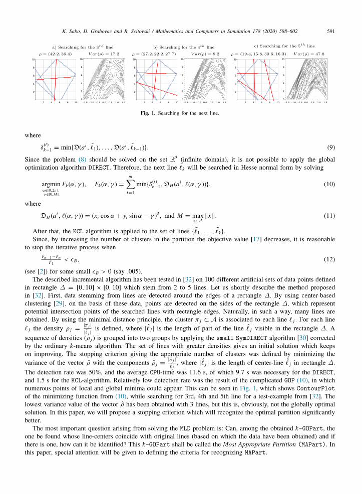
Fig. 1. Searching for the next line.

where

δ(i)k−1 = min{D(ai , ℓ1), . . . ,D(ai , ℓk−1)}. (9)

Since the problem (8) should be solved on the set R3 (infinite domain), it is not possible to apply the globaloptimization algorithm DIRECT. Therefore, the next line ℓk will be searched in Hesse normal form by solving

argminα∈[0,2π ],γ∈[0,M]

Fk(α, γ ), Fk(α, γ ) =

m∑i=1

min{δ(i)k−1,DH (ai , ℓ(α, γ ))}, (10)

where

DH (ai , ℓ(α, γ )) = (xi cosα + yi sinα − γ )2, and M = maxx∈∆

∥x∥. (11)

After that, the KCL algorithm is applied to the set of lines {ℓ1, . . . , ℓk}.Since, by increasing the number of clusters in the partition the objective value [17] decreases, it is reasonable

to stop the iterative process whenFn−1−Fn

F1< ϵB, (12)

(see [2]) for some small ϵB > 0 (say .005).The described incremental algorithm has been tested in [32] on 100 different artificial sets of data points defined

in rectangle ∆ = [0, 10] × [0, 10] which stem from 2 to 5 lines. Let us shortly describe the method proposedin [32]. First, data stemming from lines are detected around the edges of a rectangle ∆. By using center-basedclustering [29], on the basis of these data, points are detected on the sides of the rectangle ∆, which representpotential intersection points of the searched lines with rectangle edges. Naturally, in such a way, many lines areobtained. By using the minimal distance principle, the cluster π j ⊂ A is associated to each line ℓ j . For each lineℓ j the density ρ j =

|π j |

|ℓ j |is defined, where |ℓ j | is the length of part of the line ℓ j visible in the rectangle ∆. A

sequence of densities (ρ j ) is grouped into two groups by applying the small SymDIRECT algorithm [30] correctedby the ordinary k-means algorithm. The set of lines with greater densities gives an initial solution which keepson improving. The stopping criterion giving the appropriate number of clusters was defined by minimizing thevariance of the vector ρ with the components ρ j =

|π j |

|ℓ j |, where |ℓ j | is the length of center-line ℓ j in rectangle ∆.

The detection rate was 50%, and the average CPU-time was 11.6 s, of which 9.7 s was necessary for the DIRECT,and 1.5 s for the KCL-algorithm. Relatively low detection rate was the result of the complicated GOP (10), in whichnumerous points of local and global minima could appear. This can be seen in Fig. 1, which shows ContourPlotof the minimizing function from (10), while searching for 3rd, 4th and 5th line for a test-example from [32]. Thelowest variance value of the vector ρ has been obtained with 3 lines, but this is, obviously, not the globally optimalsolution. In this paper, we will propose a stopping criterion which will recognize the optimal partition significantlybetter.

The most important question arising from solving the MLD problem is: Can, among the obtained k-GOPart, theone be found whose line-centers coincide with original lines (based on which the data have been obtained) and ifthere is one, how can it be identified? This k-GOPart shall be called the Most Appropriate Partition (MAPart). Inthis paper, special attention will be given to defining the criteria for recognizing MAPart.

592 K. Sabo, D. Grahovac and R. Scitovski / Mathematics and Computers in Simulation 178 (2020) 588–602

In hard clustering problems, this partition is typically called a partition with most appropriate number of clusters,and numerous indexes are used for identifying this partition (see e.g. [4,39,41]). For solving the MLD problemor similar problems for circles, ellipses and other curves, there are numerous suggestions (see e.g. [1,9,36]) foridentifying MAPart. The ones used mostly are Calinski–Harabasz and Davies–Bouldin index. Also, we have alreadymentioned the variance stopping criterion used in [32].

3. A new incremental method for solving the MLD problem

By using (see e.g. [17])

|x | = limϵ→0+

ϵ log(2 cosh xϵ),

0 ≤ ϵ log(2 cosh xϵ) − |x | ≤ ϵ log 2, (13)

and the identity

min{x, y} =12 (x + y − |x − y|) ,

we will determine a smooth approximation Φϵk of the function Φk given in (8):

Φk(p) =12

m∑i=1

(δ

(i)k−1 + D(ai , ℓ(p)) − |D(ai , ℓ(p)) − δ

(i)k−1|

)≈

12

m∑i=1

(δ

(i)k−1 + D(ai , ℓ(p)) − ε log

(2 cosh

D(ai ,ℓ(p))−δ(i)k−1

ε

))=: Φϵ

k (p). (14)

By using such smoothing of the function Φk , we propose a simple, efficient local optimization method for solvingthe MLD problem and prove its convergence.

The following lemma shows that the difference of functions Φk and Φϵk is bounded and that, for sufficiently

small ϵ > 0, it makes sense to consider the minimization of the smooth function Φϵk instead of the minimization

of the nondifferentiable function Φk .

Lemma 1. Let ϵ > 0 and suppose that Φk : R3→ R and Φϵ

k : R3→ R are the functions given by (8) and (14),

respectively. Then:

(i) 0 ≤ Φk(p) − Φϵk (p) ≤

mϵ2 log 2

(ii) Φϵk (p) ≥ −

mϵ2 log 2, i.e. function Φϵ

k is bounded below.

Proof. Immediately from inequality (13) we have

Φk(p) − Φϵk (p) =

12

m∑i=1

(ε log

(2 cosh

D(ai ,ℓ(p))−δ(i)k−1

ε

)− |D(ai , ℓ(p)) − δ

(i)k−1|

)≤

12

m∑i=1

ϵ log 2 =mϵ2

log 2,

and consequently inequalities (i) and (ii) hold. □

3.1. The method and pseudocode of the algorithm NextLine

In the following, we define a sequence which will prove to converge to a stationary point of the functionΦϵ

k for any choice of initial approximation. Let p(0)= [ξ (0), η(0), ζ (0)]T

∈ P , and s(0)= [ξ (0), η(0)]T .Denoting

K. Sabo, D. Grahovac and R. Scitovski / Mathematics and Computers in Simulation 178 (2020) 588–602 593

ai:= [xi , yi , 1]T , let us define the following iterative process:

p(n+1)=

⎡⎢⎣ ξ (n+1)

η(n+1)

ζ (n+1)

⎤⎥⎦ =

[s(n+1)

ζ (n+1)

]=

⎡⎣ argmins,∥s∥=1

∥

√

D(n)B(n)s∥2

−ξ (n+1)x (n)− η(n+1) y(n)

⎤⎦ , n = 1, 2, . . . (15)

where

D(n)= Diag

(wϵ1(p(n)), . . . , wϵm(p(n))

), B(n)

=

⎡⎢⎣ x1 − x (n) y1 − y(n)

......

xm − x (n) ym − y(n)

⎤⎥⎦ ,wϵi (p) =

12

(1 − tanh

(pT ai

)2−δ

(i)k−1

ε

), i = 1, . . . ,m,

where δ(i)k−1 is given by (9), and

x (n)=

∑mi=1w

ϵi (p(n))xi∑m

i=1wϵi (p(n))

, y(n)=

∑mi=1w

ϵi (p(n))yi∑m

i=1wϵi (p(n))

.

According to [23], in each iteration of the optimization process (15), the solution s(n+1)= [ξ (n+1), η(n+1)]T is

equal to the right singular vector corresponding to the smaller singular value of the matrix√

D(n)B(n).

Remark 1. Note that the iterative process (15) is equivalent to the following iterative reweighted least squaresprocedure (see also e.g. [24,27])

p(n+1)= argmin

p∈P

m∑i=1

wϵi (p(n))(pT ai)2

, n = 0, 1, . . . (16)

Indeed, it follows immediately from a property of the weighted arithmetical mean that

m∑i=1

wϵi (p(n))(pT ai)2

≥

m∑i=1

wϵi (p(n))(ξ (xi − x (n)) + η(yi − y(n)))2 (17)

= ∥

√

D(n)B(n)s∥2.

Thereby the equality in (17) holds if and only if ζ = −ξ x (n)− ηy(n).

In the proof of convergence, the iterative process will be defined by (15), but in the implementation, instead ofwϵi (p), we will use the limit case ϵ → 0+, that is:

w0i (p) = lim

ϵ→0+

wϵi (p) =12

(1 − sign((pT ai )2

− δik)), i = 1, . . . ,m,

i.e. the weights are 1,0 or 0.5. From the computational point of view, the algorithm with such choice was significantlyfaster. At the same time, the experiments show that there are no differences in the quality of the results for differentvalues of ϵ.

Similarly as with the Multistart k-means algorithm (see [33]), the iterative process (15) will be initiated κ > 0times (say 5) with different random initial approximations and for the solution, we will take the one yielding thesmallest value of the function Φk . Random initial approximation will be obtained by choosing two points from theset A which will help us determine parameter-vector p ∈ P and the corresponding line ℓ(p).

The algorithm for searching for the next line according to the described procedure is stated below. Parameterϵ1 > 0 controls the number of iterations in the while-loop, in which I T ≥ 1 is the maximum number of iterations.

594 K. Sabo, D. Grahovac and R. Scitovski / Mathematics and Computers in Simulation 178 (2020) 588–602

Algorithm 2 (Next Line)

Input: A = {ai= (xi , yi ) : i = 1, . . . ,m} ⊂ ∆ ⊂ R2, ℓ1, . . . , ℓk ∈ L, I T = 15;

1: Set ai= (xi , yi , 1), i = 1, . . . ,m; i t = 0; I t = 10; ϵ1 = .005; Φ0 = +∞;

2: Define δ(i)k = min{D(ai , ℓ1), . . . ,D(ai , ℓk )}, i = 1, . . . ,m;

3: for i ter = 1 to I T do4: Randomly choose two points from A and use them to determine line ν0 with the corresponding parameter-vector

p(0)∈ P;

5: Define weights wi = .5(1 − sign(⟨p(0), ai⟩2

− δ(i)k )), i = 1, . . . ,m;

6: According to Section 2.1.1, determine the WTLS-line ν1 with parameter-vector p(1);7: Define weights wi = .5(1 − sign(⟨p(1), ai

⟩2

− δ(i)k )), i = 1, . . . ,m;

8: According to Section 2.1.1, determine the WTLS-line ν2 with parameter-vector p(2);9: while ∥p(1)

− p(2)∥ > ϵ1 and i t < I t do

10: Set p(1)= p(2);

11: Define weights wi = .5(1 − sign(⟨p(1), ai⟩2

− δ(i)k )), i = 1, . . . ,m;

12: According to Section 2.1.1, determine the WTLS-line ν2 with parameter-vector p(2);13: end while14: if Φk (p(2)) < Φ0 then15: ℓk+1 = ν2; Φ0 = Φk (p(2));16: end if17: end forOutput: {ℓ1, . . . , ℓk+1}.

Remark 2. Numerous numerical experiments on artificial datasets have shown that the iterative process can besignificantly accelerated by a modification of Step 4. Namely, it is possible to randomly choose two points from Aseveral times (say 10) and use them to determine line ν(p), corresponding parameter-vector p ∈ P and Φk(p). Withp(0) we denote the parameter-vector for which the function Φk attains the smallest value and set Φ0 = Φk(p(0)). Inthat case, the number of loops I T = 15 (see Input of Algorithm 2) can be significantly reduced (say I T = 5).

3.2. The convergence of the iterative process

Proposition 1.

(i) For every i = 1, . . . ,m and an arbitrary p ∈ P , the sequence of weights ωϵi (p) =wϵi (p)∑m

j=1 wϵj (p) , i = 1, . . . ,m,

satisfies

0 < ωϵi (p) < 1,m∑

j=1

ωϵj (p) = 1. (18)

(ii) For an arbitrary p(0)= [ξ (0), η(0), ζ (0)]T

∈ P , the sequence(p(n)

), defined by the iterative process (15), is

bounded.

Proof. The assertion (i) can be easily checked. Let us show (i i). In order to do this, note that

x (t−1)=

m∑i=1

ωϵi (p(t−1))xi , y(t−1)=

m∑i=1

ωϵi (p(t−1))yi .

By applying the Cauchy–Schwarz inequality, we have

∥p(n+1)∥

2=(ξ (n+1))2

+(η(n+1))2

+(ζ (n+1))2

= 1 +(ξ (n+1)x (n)

+ η(n+1) y(n))2

≤ 1 +

((ξ (n+1))2

+(η(n+1))2

) ((x (n))2

+(y(n))2

)

K. Sabo, D. Grahovac and R. Scitovski / Mathematics and Computers in Simulation 178 (2020) 588–602 595

= 1 +

(m∑

i=1

ωϵi (p(n))xi

)2

+

(m∑

i=1

ωϵi (p(n))yi

)2

≤ 1 +

m∑i=1

(ωϵi (p(n))

)2

(m∑

i=1

x2i +

m∑i=1

y2i

)

≤ 1 + m

(m∑

i=1

x2i +

m∑i=1

y2i

).

This implies that(p(n+1)

), defined by the iterative process (15), is bounded. □

Proposition 2. Let p(0)= [ξ (0), η(0), ζ (0)]T

∈ P and s(0)= [ξ (0), η(0)]T , and let the sequence

(p(n)

)be given by the

iterative process (15).If p(n+1)

= p(n), then Φϵk (p(n+1)) < Φϵ

k (p(n))

Proof. Let

gϵ(ϑ; p) =

m∑i=1

wϵi (p)(ϑT ai )2.

The function ϑ ↦→ gϵ(ϑ; p(n)) is a convex function and its minimizer is p(n+1). According to our assumption, wehave p(n+1)

= p(n), and therefore,

gϵ(p(n+1); p(n)) ≤ gϵ(p(n)

; p(n)). (19)

Note that the function ψ : R → R, given by ψ(x) = log(2 cosh x), is strictly convex on R and for x = y satisfiesthe gradient inequality

ψ(x) − ψ(y) > (x − y)ψ ′(y),

i.e., since ψ ′(y) = tanh y, we have

logcosh xcosh y

> (x − y) tanh y,

and consequently

ϵ logcosh

((ai )T p(n+1)

)2−δ

(i)k−1

ϵ

cosh(

(ai )T p(n))2

−δ(i)k−1

ε

> ϵ

((ai )T p(n+1)

)2−((ai )T p(n)

)2

ϵtanh

((ai )T p(n)

)2− δ

(i)k−1

ε

=

(((ai )T p(n+1))2

−((ai )T p(n))2

)tanh

((ai )T p(n)

)2− δ

(i)k−1

ε.

Finally,

Φϵk (p(n+1)) − Φϵ

k (p(n)) =12

m∑i=1

⎛⎜⎝((ai )T p(n+1))2−((ai )T p(n))2

− ϵ logcosh

((ai )T p(n+1)

)2−δ

(i)k−1

ϵ

cosh(

(ai )T p(n))2

−δ(i)k−1

ε

⎞⎟⎠< 1

2

m∑i=1

(((ai )T p(n+1))2

−((ai )T p(n))2

)(1−tanh

((ai )T p(n)

)2− δ

(i)k−1

ε

)

=

m∑i=1

(((ai )T p(n+1))2

−((ai )T p(n))2

)wϵi (p(n))

=(gϵ(p(n+1)

; p(n)) − gϵ(p(n); p(n))

)≤ 0. □

596 K. Sabo, D. Grahovac and R. Scitovski / Mathematics and Computers in Simulation 178 (2020) 588–602

Theorem 1. Let p(0)= [ξ (0), η(0), ζ (0)]T

∈ P , and s(0)= [ξ (0), η(0)]T , and let the sequence

(p(n)

)be given by the

iterative process (15). Then

(i) The sequence(p(n)

)has an accumulation point.

(ii) The sequence((Φϵ

k

)(n))

, where(Φϵ

k

)(n):= Φϵ

k (p(n)), converges.

(iii) Every accumulation point p of the sequence(p(n)

)is a stationary point of the functional Φϵ

k .(iv) If p1 and p2 are two accumulation points of the sequence

(p(n)

), then Φϵ

k (p1) = Φϵk (p2).

Proof. (i) According to Proposition 1, the sequence(p(n)

)is bounded, and therefore it has an accumulation point.

(i i) According to Proposition 2, the sequence(Φϵ(n)

k

)is monotonously decreasing, and by Lemma 1, the

functional Φϵk is bounded below. Therefore, there exists Φϵ⋆

k , such that Φϵ⋆k = limn→∞Φϵ(n)

k .(i i i) Let us suppose that p is an accumulation point of the sequence

(p(n)

), i.e.

p = [ξ , η, ζ ]T= argmin

p∈Pgϵ(p; p).

Then p is a stationary point of the function gϵ(·; p), i.e. ∇p,λLgϵ (p, λ; p) = 0, where

∇p,λLgϵ (p, λ; p) =

⎡⎢⎢⎢⎢⎣2∑m

i=1wϵi (p)

(pT ai

)xi + 2λξ

2∑m

i=1wϵi (p)

(pT ai

)yi + 2λη

2∑m

i=1wϵi (p)

(pT ai

)ξ 2

+ η2− 1

⎤⎥⎥⎥⎥⎦ ,and

Lgϵ (p, λ; p) = gϵ(p; p) + λ(ξ 2+ η2

− 1),

is the corresponding Lagrange function.On the other hand,

∇p,λLΦϵk(p; λ) =

⎡⎢⎢⎢⎣2∑m

i=1wϵi (p)

(pT ai

)xi + 2λξ

2∑m

i=1wϵi (p)

(pT ai

)yi + 2λη

2∑m

i=1wϵi (p)

(pT ai

)ξ 2

+ η2− 1

⎤⎥⎥⎥⎦ ,where

LΦϵk(p; λ) = Φϵ

k (p) + λ(ξ 2+ η2

− 1),

is the corresponding Lagrange function.Finally,

∇p,λLgϵ (p, λ; p) = ∇p,λLΦϵk(p; λ) = 0,

i.e. p is a stationary point of the functional Φϵk .

(iv) Let(

p(n)1

)and

(p(n)

2

)be two subsequences of the sequence

(p(n)

), such that p1 = limn→∞p(n)

1 and

p2 = limt→∞ p(n)2 . Since the sequence

(Φϵ(n)

k

)converges, we have

Φϵk (p1) = lim

t→∞Φϵ

k (p(n)1 ) = lim

t→∞Φϵ

k (p(n)2 ) = Φϵ

k (p2). □

4. A new incremental algorithm for the MLD problem

Using the method described in Section 3, we will construct a new incremental algorithm for multiple linedetection by successive application of Algorithm 2. However, the stopping criterion (12) may not always be suitable.It may happen that this condition allows less or significantly more iterations in incremental algorithm, which can,as a result, have smaller or bigger distance from MAPart and significantly longer computing time. Therefore, weshall complement the stopping criterion (12) with a more precise condition.

K. Sabo, D. Grahovac and R. Scitovski / Mathematics and Computers in Simulation 178 (2020) 588–602 597

4.1. The stopping criterion

By using the approach from the DBSCAN-algorithm (see e.g. [6,35,44,47]), for the given Min Pts > 2 and forevery a ∈ A, let ϵa > 0 be the radius of the smallest disc centered at a and containing Min Pts elements of theset A. Based on this information, we will define the ϵ-density of the set A.

Definition 1. Let R(A) = {ϵa : a ∈ A}. We define ϵ-density of the set A to be the 99% quantile of the set R(A)and denote it by ϵ(A).

Note that for almost all points a ∈ A, the corresponding disc with center a and radius ϵ(A) contains at leastMin Pts elements from the set A.

Let Π (k) be the partition obtained in step k of the iterative process. For each cluster π ∈ Π (k) with line-centerℓ(p) let

V (π ) := {D1(ai , ℓ(p)) : ai∈ π}, (20)

where D1(ai , ℓ(p)) = |ξ xi + ηyi + ζ | is the ordinary Euclidean distance from the point ai= (xi , yi ) ∈ π to the

line ℓ(p). We define Quantile of the Data to Line Deviations (QD) of cluster π as 90% quantile of the set V (π ).We expect that the partition Π (k) is near k-GOPart if:

QD[π ] < ϵ(A), ∀π ∈ Π (k). (21)

Therefore, the stopping criterion (12) can be complemented with the condition (21).Note that the condition (21) will be easier to fulfill if QD[π ] is defined as p% (p < 90) quantile of the set V (π ).

In this way, we can influence the number of lines that will appear in the output of the incremental algorithm.

4.2. The construction of the new algorithm

First, for the given data set A, we determine parameter Min Pts(A) := ⌊log |A|⌋ according to [5] and parameterϵB which, according to [3], limits the maximum number of iterations. Starting with TLS-line, we determine the nextline in every subsequent step by applying Algorithm 2 until the stopping condition (21) or (12) is met.

Algorithm 3 (A new incremental algorithm for line detection)

Input: A = {ai= (xi , yi ) : i = 1, . . . ,m} ⊂ ∆ ⊂ R2;

1: Set ϵB = .005; Min Pts = ⌊log |A|⌋;2: Determine ϵ-density, ϵ(A) according to Definition 1;3: According to Section 2.1.1, determine the WTLS-line ℓ1 and the objective function value F1;4: By using Algorithm 2, determine the next line ℓ2 and set k = 2;5: Apply the KCL algorithm to the lines ℓ1, ℓ2 and denote the obtained partition by

Π (2)= {π1(ℓ1), π2(ℓ2)} and the objective function value by F2;

6: Determine QD[π j ], j = 1, 2, as 90% quantile of the set V (π j ) given by (20);7: while max

j=1,...,kQD[π j ] > ϵ(A) and (Fk−1 − Fk )/F1 > ϵB do

8: By using Algorithm 2, determine the next line ℓk+19: Apply the KCL algorithm to the lines ℓ1, . . . , ℓk+1 and denote the obtained partition by

Π (k+1)= {π1(ℓ1), . . . , πk+1(ℓk+1)} and the objective function value by Fk+1;

10: Determine QD[π j ], j = 1, . . . , k + 1, as 90% quantile of the set V (π j ) given by (20);11: Set k := k + 1 and Fk := Fk+1;12: end whileOutput: {ℓ1, . . . , ℓk , ℓk+1}.

4.3. Searching for the most appropriate partition

Since the incremental method described in Section 3 is of local character and it depends on the choice ofinitial points in Algorithm 2, Algorithm 3 will most commonly produce more lines than can be expected from

598 K. Sabo, D. Grahovac and R. Scitovski / Mathematics and Computers in Simulation 178 (2020) 588–602

the configuration of the set A. Hence, the obtained partition is not always MAPart too. This indicates the necessityof eliminating some center-lines from this partition.

We will assume that the data points coming from some line ℓ, not known in advance, satisfy the homogeneityassumption, i.e. we assume that these points are scattered around line ℓ as if they were obtained by adding noiseto the points uniformly distributed along the line segment of ℓ contained in rectangle ∆. We say that such dataare homogeneously scattered around line ℓ. In Section 5, we use this approach to construct synthetic data sets fortesting. There we use bivariate normal distribution with mean zero to model the noise. First, we define the termlocal density of the cluster.

Definition 2. Let π (ℓ) ∈ Π (k) be a cluster of data points obtained from a line ℓ ∈ L and let |ℓ| be the length ofcenter-line ℓ in rectangle ∆. The number ρ(π ) =

|π |

|ℓ|will be called the local density of the cluster π .

Since, for each a ∈ A, the corresponding disc with radius ϵ(A) contains at least Min Pts elements from the setA, the lower bound of the local density for each cluster π ∈ Π (k) can be estimated by

ρ(π ) ≥Min Pts2ϵ(A) . (22)

Therefore, the partition Π (k)= {π1(ℓ1), . . . , πk(ℓk)}, obtained from Algorithm 3, will not be MAPart if (22) does

not hold for at least one π ∈ Π (k).For each cluster π = π (ℓ) ∈ Π (k), for which (22) does not hold, the corresponding line-center ℓ should be

dropped. Elements of these clusters should be distributed to other clusters by using the minimal distance principle.

4.3.1. Necessary conditions for the most appropriate partitionWe are now in the position to define necessary conditions for the partition Π (k) to be MAPart as well:

A0: QD[π ] < ϵ(A) for all clusters π ∈ Π (k);A1: ρ(π ) ≥

Min Pts2ϵ(A) for all clusters π ∈ Π (k).

Remark 3. The stated necessary conditions for MAPart could be easily adapted in other situations while solvingsimilar problems: multiple circle detection problem [31,33], multiple ellipse detection problem [1,9], multiplegeneralized circle detection problem [34], multiple segment detection problem [40], etc.

4.3.2. The solution correctionLet Π (κ) be the partition obtained by executing Algorithm 3 and leaving out center-lines that do not satisfy

condition A1. Typically, it will happen that some of the obtained center-lines no longer meet the condition A0, andso, those lines should be left out too. In this way, we obtain κ1 ≤ κ lines ℓs , s = 1, . . . , κ1, to which we associatethe sets

πs = {a ∈ A : D1(a, ℓs) ≤ ϵ(A)}, s = 1, . . . , κ1,

and we can define the set

B = A \

κ1⋃s=1

πs . (23)

If B = ∅, we will again run Algorithm 3 on it with the same parameters Min Pts and ϵ(A).The obtained partition with κ2 clusters Π (κ2)(B) usually has significantly less clusters, which, however, can have

low density regions. Therefore, we drop center-lines of those clusters π ∈ Π (κ2)(B) for which the correspondingcondition A1 is not fulfilled, i.e. for which ρ(π ) ≥

Min Pts2ϵ(B) does not hold.

By applying the KCL-algorithm to center-lines obtained in this way together with center-lines ℓs , s = 1, . . . , κ1,we expect to get MAPart, which can be checked by using necessary conditions A0 and A1.

5. Illustrating and testing the algorithm

Algorithm 3 will be investigated together with checking the necessary conditions for the MAPart defined inSection 4.3.1 and performing the necessary corrections described in Section 4.3.2.

K. Sabo, D. Grahovac and R. Scitovski / Mathematics and Computers in Simulation 178 (2020) 588–602 599

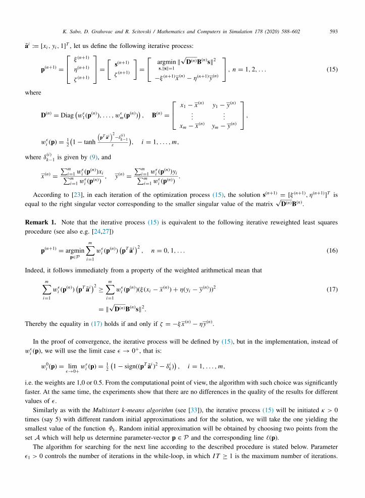
Fig. 2. Results of Algorithm 3.

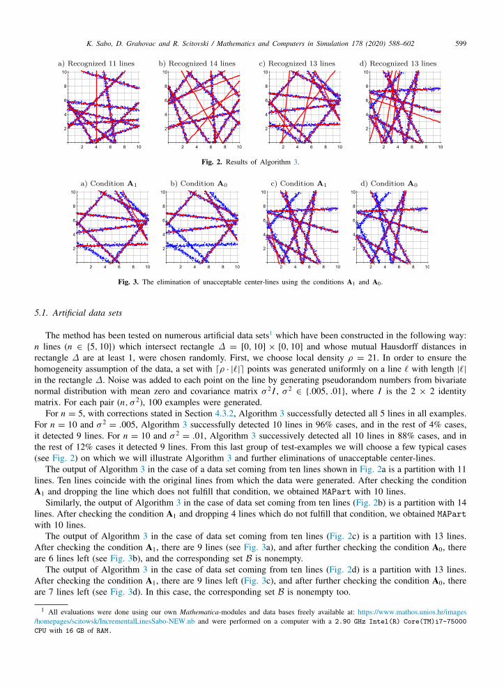
Fig. 3. The elimination of unacceptable center-lines using the conditions A1 and A0.

5.1. Artificial data sets

The method has been tested on numerous artificial data sets1 which have been constructed in the following way:n lines (n ∈ {5, 10}) which intersect rectangle ∆ = [0, 10] × [0, 10] and whose mutual Hausdorff distances inrectangle ∆ are at least 1, were chosen randomly. First, we choose local density ρ = 21. In order to ensure thehomogeneity assumption of the data, a set with ⌈ρ · |ℓ|⌉ points was generated uniformly on a line ℓ with length |ℓ|

in the rectangle ∆. Noise was added to each point on the line by generating pseudorandom numbers from bivariatenormal distribution with mean zero and covariance matrix σ 2 I , σ 2

∈ {.005, .01}, where I is the 2 × 2 identitymatrix. For each pair (n, σ 2), 100 examples were generated.

For n = 5, with corrections stated in Section 4.3.2, Algorithm 3 successfully detected all 5 lines in all examples.For n = 10 and σ 2

= .005, Algorithm 3 successfully detected 10 lines in 96% cases, and in the rest of 4% cases,it detected 9 lines. For n = 10 and σ 2

= .01, Algorithm 3 successively detected all 10 lines in 88% cases, and inthe rest of 12% cases it detected 9 lines. From this last group of test-examples we will choose a few typical cases(see Fig. 2) on which we will illustrate Algorithm 3 and further eliminations of unacceptable center-lines.

The output of Algorithm 3 in the case of a data set coming from ten lines shown in Fig. 2a is a partition with 11lines. Ten lines coincide with the original lines from which the data were generated. After checking the conditionA1 and dropping the line which does not fulfill that condition, we obtained MAPart with 10 lines.

Similarly, the output of Algorithm 3 in the case of data set coming from ten lines (Fig. 2b) is a partition with 14lines. After checking the condition A1 and dropping 4 lines which do not fulfill that condition, we obtained MAPart

with 10 lines.The output of Algorithm 3 in the case of data set coming from ten lines (Fig. 2c) is a partition with 13 lines.

After checking the condition A1, there are 9 lines (see Fig. 3a), and after further checking the condition A0, thereare 6 lines left (see Fig. 3b), and the corresponding set B is nonempty.

The output of Algorithm 3 in the case of data set coming from ten lines (Fig. 2d) is a partition with 13 lines.After checking the condition A1, there are 9 lines left (Fig. 3c), and after further checking the condition A0, thereare 7 lines left (see Fig. 3d). In this case, the corresponding set B is nonempty too.

1 All evaluations were done using our own Mathematica-modules and data bases freely available at: https://www.mathos.unios.hr/images/homepages/scitowsk/IncrementalLinesSabo-NEW.nb and were performed on a computer with a 2.90 GHz Intel(R) Core(TM)i7-75000

CPU with 16 GB of RAM.

600 K. Sabo, D. Grahovac and R. Scitovski / Mathematics and Computers in Simulation 178 (2020) 588–602

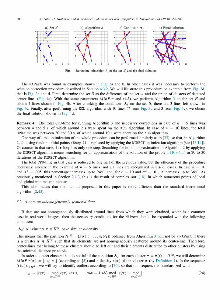
Fig. 4. Rerunning Algorithm 3 on the set B and the final solution.

The MAPart was found in examples shown in Fig. 2a and b. In other cases it was necessary to perform thesolution correction procedure described in Section 4.3.2. We will illustrate this procedure on example from Fig. 2d,that is Fig. 3c and d. First, determine the set B as the difference of the set A and the union of clusters of detectedcenter-lines (Fig. 4a). With the same parameters Min Pts and ϵ(A), we perform Algorithm 3 on the set B andobtain 4 lines shown in Fig. 4b. After checking the conditions A1 on the set B, there are 3 lines left shown inFig. 4c. Finally, after performing the KCL algorithm with 10 lines (7 from Fig. 3d and 3 from Fig. 4c), we obtainthe final solution shown in Fig. 4d.

Remark 4. The total CPU-time for running Algorithm 3 and necessary corrections in case of n = 5 lines wasbetween 4 and 5 s, of which around 2 s were spent on the KCL algorithm. In case of n = 10 lines, the totalCPU-time was between 20 and 30 s, of which around 10 s were spent on the KCL algorithm.

One way of time optimization of the whole procedure can be performed similarly as in [33], so that, in Algorithm2, choosing random initial points (Step 4) is replaced by applying the DIRECT optimization algorithm (see [13,14]).Of course, in that case, for-loop has only one step. Searching for initial approximation in Algorithm 2 by applyingthe DIRECT algorithm means searching for an approximation of the solution of the problem (10)–(11) in 20 to 30iterations of the DIRECT algorithm.

The total CPU-time in that case is reduced to one half of the previous value, but the efficiency of the proceduredecreases: already in the example of n = 5 lines, not all lines are recognized in 8% of cases. In case n = 10and σ 2

= .005, this percentage increases up to 24%, and, for n = 10 and σ 2= .01, it increases up to 36%. As

previously mentioned in Section 2.1.3, this is the result of complex GOP (10), in which numerous points of localand global minima can appear.

This also means that the method proposed in this paper is more efficient than the standard incrementalalgorithm [2,43].

5.2. A note on inhomogeneously scattered data

If data are not homogeneously distributed around lines from which they were obtained, which is a commoncase in real-world images, then the necessary conditions for the MAPart should be expanded with the followingcondition:

A2: All clusters π ∈ Π (k) have similar ϵ-density.

This means that the partition Π (k)= {π1(ℓ1), . . . , πk(ℓk)} obtained from Algorithm 3 will not be a MAPart if there

is a cluster π ∈ Π (k) such that its elements are not homogeneously scattered around its center-line. Therefore,center-lines that belong to these clusters should be left out and their elements distributed to other clusters by usingthe minimal distance principle.

In order to detect clusters that do not fulfill the condition A2, for each cluster π = π (ℓ) ∈ Π (k), we will determineMin Pts(π ) := ⌊log |π |⌋ (according to [5]) and ϵ-density ϵ(π ) of the cluster π (by Definition 1). In the sequence(ϵ(π ))π∈Π (k) , we will try to identify outliers according to [26], so that this sequence is standardized with

νπ := |ϵ(π ) − medπ∈Π (k)

ϵ(π )|/MAD, MAD = 1.483 medπ∈Π (k)

⏐⏐ϵ(π ) − medπ∈Π (k)

⏐⏐. (24)

K. Sabo, D. Grahovac and R. Scitovski / Mathematics and Computers in Simulation 178 (2020) 588–602 601

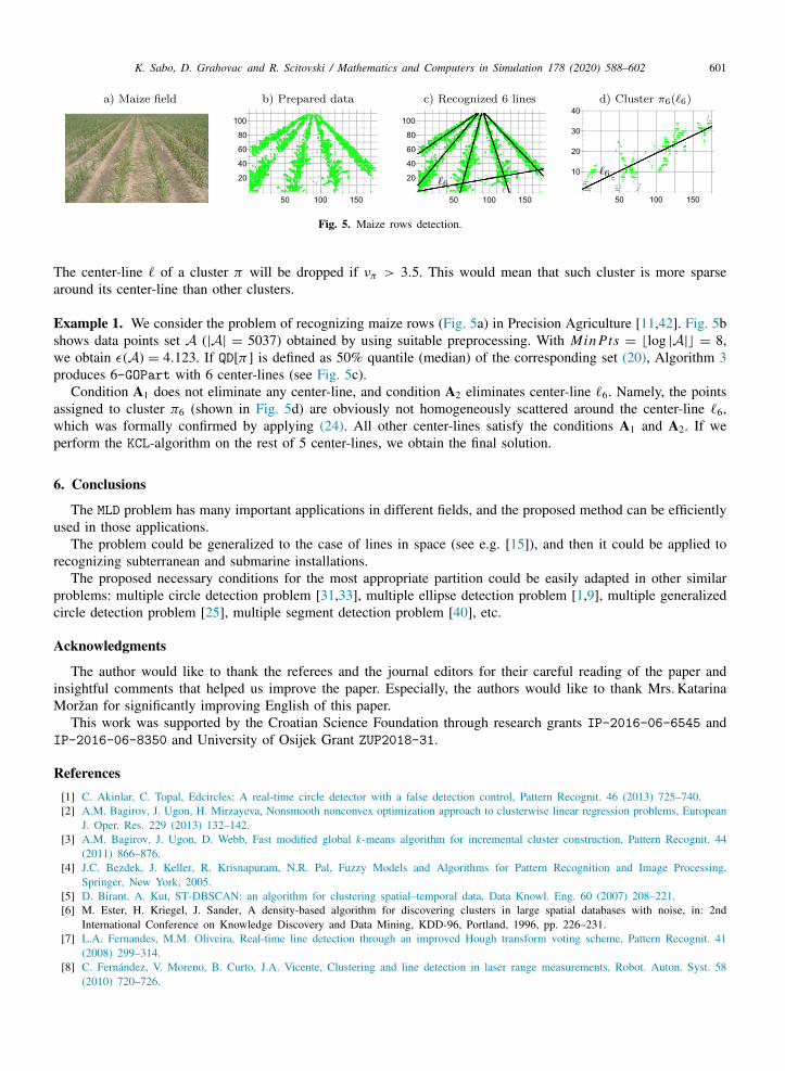
Fig. 5. Maize rows detection.

The center-line ℓ of a cluster π will be dropped if νπ > 3.5. This would mean that such cluster is more sparsearound its center-line than other clusters.

Example 1. We consider the problem of recognizing maize rows (Fig. 5a) in Precision Agriculture [11,42]. Fig. 5bshows data points set A (|A| = 5037) obtained by using suitable preprocessing. With Min Pts = ⌊log |A|⌋ = 8,we obtain ϵ(A) = 4.123. If QD[π ] is defined as 50% quantile (median) of the corresponding set (20), Algorithm 3produces 6-GOPart with 6 center-lines (see Fig. 5c).

Condition A1 does not eliminate any center-line, and condition A2 eliminates center-line ℓ6. Namely, the pointsassigned to cluster π6 (shown in Fig. 5d) are obviously not homogeneously scattered around the center-line ℓ6,which was formally confirmed by applying (24). All other center-lines satisfy the conditions A1 and A2. If weperform the KCL-algorithm on the rest of 5 center-lines, we obtain the final solution.

6. Conclusions

The MLD problem has many important applications in different fields, and the proposed method can be efficientlyused in those applications.

The problem could be generalized to the case of lines in space (see e.g. [15]), and then it could be applied torecognizing subterranean and submarine installations.

The proposed necessary conditions for the most appropriate partition could be easily adapted in other similarproblems: multiple circle detection problem [31,33], multiple ellipse detection problem [1,9], multiple generalizedcircle detection problem [25], multiple segment detection problem [40], etc.

Acknowledgments

The author would like to thank the referees and the journal editors for their careful reading of the paper andinsightful comments that helped us improve the paper. Especially, the authors would like to thank Mrs. KatarinaMorzan for significantly improving English of this paper.

This work was supported by the Croatian Science Foundation through research grants IP-2016-06-6545 andIP-2016-06-8350 and University of Osijek Grant ZUP2018-31.

References[1] C. Akinlar, C. Topal, Edcircles: A real-time circle detector with a false detection control, Pattern Recognit. 46 (2013) 725–740.[2] A.M. Bagirov, J. Ugon, H. Mirzayeva, Nonsmooth nonconvex optimization approach to clusterwise linear regression problems, European

J. Oper. Res. 229 (2013) 132–142.[3] A.M. Bagirov, J. Ugon, D. Webb, Fast modified global k-means algorithm for incremental cluster construction, Pattern Recognit. 44

(2011) 866–876.[4] J.C. Bezdek, J. Keller, R. Krisnapuram, N.R. Pal, Fuzzy Models and Algorithms for Pattern Recognition and Image Processing,

Springer, New York, 2005.[5] D. Birant, A. Kut, ST-DBSCAN: an algorithm for clustering spatial–temporal data, Data Knowl. Eng. 60 (2007) 208–221.[6] M. Ester, H. Kriegel, J. Sander, A density-based algorithm for discovering clusters in large spatial databases with noise, in: 2nd

International Conference on Knowledge Discovery and Data Mining, KDD-96, Portland, 1996, pp. 226–231.[7] L.A. Fernandes, M.M. Oliveira, Real-time line detection through an improved Hough transform voting scheme, Pattern Recognit. 41

(2008) 299–314.[8] C. Fernández, V. Moreno, B. Curto, J.A. Vicente, Clustering and line detection in laser range measurements, Robot. Auton. Syst. 58

(2010) 720–726.

602 K. Sabo, D. Grahovac and R. Scitovski / Mathematics and Computers in Simulation 178 (2020) 588–602

[9] R. Grbic, D. Grahovac, R. Scitovski, A method for solving the multiple ellipses detection problem, Pattern Recognit. 60 (2016)824–834.

[10] R. Grbic, E.K. Nyarko, R. Scitovski, A modification of the DIRECT method for Lipschitz global optimization for a symmetric function,J. Global Optim. 57 (2013) 1193–1212.

[11] J. Guerrero, G. Pajares, M. Montalvo, J. Romeo, M. Guijarro, Support vector machines for crop/weeds identification in maize fields,Expert Syst. Appl. 39 (2012) 11149–11155.

[12] R. Horst, H. Tuy, Global Optimization: Deterministic Approach, third, revised and enlarged ed., Springer, 1996.[13] D.R. Jones, The direct global optimization algorithm, in: C.A. Floudas, P.M. Pardalos (Eds.), The Encyclopedia of Optimization, Kluwer

Academic Publishers, Dordrect, 2001, pp. 431–440.[14] D.R. Jones, C.D. Perttunen, B.E. Stuckman, Lipschitzian optimization without the Lipschitz constant, J. Optim. Theory Appl. 79 (1993)

157–181.[15] D. Jukic, R. Scitovski, Š. Ungar, The best total least squares line in R3, in: I. Aganovic, T. Hunjak, R. Scitovski (Eds.), Proceedings

of the 7th International Conference on Operational Research KOI98, 1999, pp. 311–316.[16] H. Kälviäinen, P. Hirvonen, L. Xu, E. Oja, Probabilistic and non-probabilistic Hough transforms: overview and comparison, Image

Vis. Comput. 13 (1995) 239–252.[17] J. Kogan, Introduction to Clustering Large and High-Dimensional Data, Cambridge University Press, New York, 2007.[18] D.E. Kvasov, Y.D. Sergeyev, Lipschitz gradients for global optimization in a one-point-based partitioning scheme, J. Comput. Appl.

Math. 236 (2012) 4042–4054.[19] M. Locatelli, F. Schoen, Global Optimization: Theory, Algorithms, and Applications, SIAM and the Mathematical Optimization Society,

2013.[20] A. Manzanera, T.P. Nguyen, X. Xu, Line and circle detection using dense one-to-one Hough transforms on greyscale images, EURASIP

J. Image Video Process. (2016) http://dx.doi.org/10.1186/s13640-016-0149-y.[21] I. Markovsky, M.L. Rastello, A. Premoli, A. Kukush, S.V. Huffel, The element-wise weighted total least-squares problem, Comput.

Statist. Data Anal. 50 (2006) 181–209.[22] P. Mukhopadhyay, B.B. Chaudhuri, A survey of Hough transform, Pattern Recognit. 48 (2015) 993–1010.[23] Y. Nievergelt, Total least squares: state-of-the-art regression in numerical analysis, SIAM Rev. 36 (1994) 258–264.[24] M.R. Osborne, Finite Algorithms in Optimization and Data Analysis, John Wiley, Chichester, 1985.[25] U. Radojicic, R. Scitovski, K. Sabo, A fast and efficient method for solving the multiple closed curve detection problem, in: M.D.

Marsico, G.S. di Baja, A. Fred (Eds.), Proceedings of the 8th International Conference on Pattern Recognition Applications andMethods - Vol. 1: ICPRAM, Prague, Czech Republic, volume 1 - 978-989-758-351-3, 2019, pp. 269–276.

[26] P.J. Rousseeuw, M. Hubert, Robust statistics for outlier detection, Wiley Interdiscip. Rev. Data Min. Knowl. Discov. 1 (2011) 73–79.[27] K. Sabo, R. Scitovski, The best least absolute deviations line – properties and two efficient methods, ANZIAM J. 50 (2008) 185–198.[28] K. Sabo, R. Scitovski, An approach to cluster separability in a partition, Inform. Sci. 305 (2015) 208–218.[29] K. Sabo, R. Scitovski, I. Vazler, One-dimensional center-based l1-clustering method, Optim. Lett. 7 (2013) 5–22.[30] R. Scitovski, A new global optimization method for a symmetric Lipschitz continuous function and application to searching for a

globally optimal partition of a one-dimensional set, J. Global Optim. 68 (2017) 713–727.[31] R. Scitovski, T. Maroševic, Multiple circle detection based on center-based clustering, Pattern Recognit. Lett. 52 (2014) 9–16.[32] R. Scitovski, U. Radojicic, K. Sabo, A fast and efficient method for solving the multiple line detection problem, Rad HAZU, Mat.

Znan. 23 (2019) 123–140.[33] R. Scitovski, K. Sabo, Application of the DIRECT algorithm to searching for an optimal k-partition of the set A and its application

to the multiple circle detection problem, J. Global Optim. 74 (1) (2019) 63–77.[34] R. Scitovski, K. Sabo, A combination of k-means and dbscan algorithm for solving the multiple generalized circle detection problem,

Adv. Data Anal. Classif. (2020) http://dx.doi.org/10.1007/s11634-020-00385-9.[35] R. Scitovski, K. Sabo, DBSCAN-like clustering method for various data densities, Pattern Anal. Appl. 23 (2020) 541–554, http:

//dx.doi.org/10.1007/s10044-019-00809-z.[36] R. Scitovski, S. Scitovski, A fast partitioning algorithm and its application to earthquake investigation, Comput. Geosci. 59 (2013)

124–131.[37] H. Späth, Algorithm 48: a fast algorithm for clusterwise linear regression, Computing 29 (1981) 17–181.[38] H. Späth, Cluster-Formation und Analyse, R. Oldenburg Verlag, München, 1983.[39] S. Theodoridis, K. Koutroumbas, Pattern Recognition, fourth ed., Academic Press, Burlington, 2009.[40] J.C.R. Thomas, A new clustering algorithm based on k-means using a line segment as prototype, in: C.S. Martin, S.-W. Kim (Eds.),

Progress in Pattern Recognition, Image Analysis, Computer Vision, and Applications, Springer Berlin Heidelberg, 2011, pp. 638–645.[41] L. Vendramin, R.J.G.B. Campello, E.R. Hruschka, On the comparison of relative clustering validity criteria, in: Proceedings of the

SIAM International Conference on Data Mining, SDM 2009, April 30 – May 2, 2009, Sparks, Nevada, USA, SIAM, 2009, pp.733–744.

[42] I. Vidovic, R. Cupec, e. Hocenski, Crop row detection by global energy minimization, Pattern Recognit. 55 (2016) 68–86.[43] I. Vidovic, R. Scitovski, Center-based clustering for line detection and application to crop rows detection, Comput. Electron. Agric.

109 (2014) 212–220.[44] P. Viswanath, V.S. Babu, Rough-DBSCAN: a fast hybrid density based clustering method for large data sets, Pattern Recognit. Lett.

30 (2009) 1477–1488.[45] T. Weise, Global Optimization Algorithms. Theory and Application, e-book, 2008, http://www.it-weise.de/projects/book.pdf.[46] L. Xu, E. Oja, P. Kultanen, A new curve detection method: Randomized Hough Transform (RHT), Pattern Recognit. Lett. 11 (1990)

331–338.[47] Y. Zhu, K.M. Ting, M.J. Carman, Density-ratio based clustering for discovering clusters with varying densities, Pattern Recognit. 60

(2016) 983–997.