Incremental Elliptical Boundary Estimation for Anomaly Detection inWireless Sensor Networks

Masud Moshtaghi∗, Christopher Leckie∗, Shanika Karunasekera∗, James C. Bezdek†,Sutharshan Rajasegarar‡ and Marimuthu Palaniswami‡

∗NICTA Victoria Research LaboratoriesDepartment of Computer Science and Software Engineering, The University of Melbourne, Australia

†Department of Computer Science and Software EngineeringThe University of Melbourne, Australia

‡Department of Electrical and Electronic EngineeringThe University of Melbourne, Australia

I. ABSTRACT

Wireless Sensor Networks (WSNs) provide a low costoption for gathering spatially dense data from different en-vironments. However, WSNs have limited energy resourcesthat hinder the dissemination of the raw data over thenetwork to a central location. This has stimulated researchinto efficient data mining approaches, which can exploitthe restricted computational capabilities of the sensors tomodel their normal behavior. Having a normal model of thenetwork, sensors can then forward anomalous measurementsto the base station. Most of the current data modelingapproaches proposed for WSNs require a fixed offline train-ing period and use batch training in contrast to the realstreaming nature of data in these networks. In addition theyusually work in stationary environments. In this paper wepresent an efficient online model construction algorithm thatcaptures the normal behavior of the system. Our model iscapable of tracking changes in the data distribution in themonitored environment. We illustrate the proposed algorithmwith numerical results on both real-life and simulated datasets, which demonstrate the efficiency and accuracy of ourapproach compared to existing methods. Keywords-AnomalyDetection; Streaming Data Analysis; Incremental EllipticalBoundary Estimation; IDCAD;

II. INTRODUCTION

A Wireless Sensor Network (WSN) consists of a set ofnodes each equipped with a set of sensing devices. WSNsprovide a cost-effective platform for monitoring and datacollection in environments where the deployment of wiredsensing infrastructure is too expensive or impractical [1].The different sensing elements installed on each node, forexample temperature and humidity sensors, enable the WSNto collect a large volume of multidimensional and correlatedsamples. An important challenge for WSNs is to detectunusual measurements, which are caused by either eventsof interest in the surrounding environment or faults in thenodes. Detection of anomalous measurements at the nodesallows us to conserve limited resources of the wirelessnodes by reducing the communication of raw data over the

network. In order to detect anomalies we need a well-definednotion of the normal behavior of the nodes.

Various data mining approaches have been proposed tobuild a model of the normal behavior of the nodes. In adecentralized approach, each node in WSNs builds a localmodel of its own normal behavior. The parameters of thelocal models are forwarded to the base station or the clusterhead where a global model is calculated based on the localmodels. Many different data modeling methods using thisapproach have been proposed recently. However, most ofthese models are static models and cannot adapt to changesin the environment [2], [3], [4], [5], [6], [7], [8]. Moreover,their accuracy depends on proper selection of the initialtraining period. If the initial training period is not a goodrepresentative of future measurements, the model fails. Anopen research issue is how to continuously learn models ofnormal behavior in non-stationary environments. The focusof this paper is on efficient anomaly detection techniquessuitable for resource constrained wireless sensor nodes todetect unusual events in non-stationary environments.

While anomaly detection is an active research topic inWSNs, a critical issue for the practical use of anomalydetection techniques is how to generalize their use to onlinedata streams with temporal changes. There are well-knownbatch techniques for anomaly detection in multidimensionaldata which use Mahalanobis distance for anomaly detection([9] and [10]). In particular, the authors of [5] proposed ahyperellipsoidal boundary using Mahalanobis distance calledData Capture Anomaly Detection (DCAD) to compute alocal model of the normal data in WSNs. In this paper,we build on the static model of [5] to propose an iterativeapproximation of the Mahalanobis distance and the hyper-ellipsoidal boundary in data streaming environments.

This paper offers three contributions: (1) introduction ofan iterative formula for the estimation of an ellipsoidalboundary, iterative DCAD (IDCAD); (2) introduction of aforgetting factor method to increase the tracking capabilitiesof the model in non-stationary environments; and (3) an

2011 11th IEEE International Conference on Data Mining

1550-4786/11 $26.00 © 2011 IEEE

DOI 10.1109/ICDM.2011.80

467

empirical evaluation of the performance of the proposedapproaches on three real-life and two synthetic datasets. Ourresults demonstrate that the new approach, by adapting tochanges in the environment, can achieve higher accuracythan an existing batch approach in non-stationary environ-ments which makes it more suitable for use in practicalapplications. In contrast to the batch approach, our iter-ative approach does not require all previous raw data tobe buffered at the sensor nodes, thus reducing memoryoverhead. We also show that in the evaluation datasets,the proposed iterative formula without the forgetting factorterminates at the same ellipsoid as the batch approach.The next section summarizes related work. In Section IVwe present the notation used in this paper. In SectionV we derive the formulas for iterative adjustment of thehyperellipsoidal boundary. Section VI develops the methodthat adds tracking capability to the IDCAD. In Section VIIwe evaluate our method on five datasets. A summary andconclusions are given in Section VIII.

III. BACKGROUND AND RELATED WORK

An important challenge in monitoring systems is to detectunexpected events or unusual behavior. Therefore, anomalydetection techniques are an important part of automatedmonitoring systems. In WSNs, anomaly detection techniqueshave been applied in a variety of applications [11], includingintrusion detection [12], event detection [13] and qualityassurance [14], [15]. Numerous factors affect the use ofanomaly detection in these applications, such as mobilityin sensors, the condition of the environment (benign oradverse) [16], the dynamics of the environment, and energyconstraints. In order to detect anomalies in the data weneed to separate them from normal observations. The mostcommon way to perform this task is by modeling the normaldata and then identifying deviations from the model.

The authors of [17] proposed one class support vectormachine models to find anomalies in WSN data. The mainassumption in this approach is that all the training datais available at the sensors, and the training can be donein batch mode, i.e., all the measurements collected areprocessed as a single batch. Although these methods oftenprovide a good decision boundary for the normal data,they impose a computational overhead of O(n3) on eachsensor. The authors of [18] proposed a Discrete WaveletTransform (DWT) combined with a self-organizing map(SOM) technique to detect anomalies. The DWT encodedthe measurements at the nodes, and the SOM was used atthe base station to detect unusual sets of wavelet coefficients.The main drawbacks of this method are firstly, SOM trainingis sensitive to noise in the data and secondly, it is hardto understand what triggered the reported anomaly. Thealarms generated by the anomaly detection systems usuallyrequire further verification by more expensive measures suchas human operators or fault diagnostic systems. Accepted

alarms can then be used as a trigger for other tasks suchas waking up more sensors in the field, or increasing thesampling rate of the sensors to gather more data. Therefore,it is important that the output of an anomaly detectiontechnique be easy to interpret.

In [3], [5] hyperellipsoidal boundaries are used to modelthe normal behavior of the system with batch training. Thismethod tolerates noise in the training data and individualanomalies are reported to users. However, the hyperellip-soidal boundaries are calculated over a training period. Themethods in [3], [5] require the nodes to keep measurementsin the memory during the training period, and further, atthe end of training all measurements are processed in batchmode. These methods are computationally efficient, but theirinability to adapt to changes in the environment and theproblem of choosing a proper training period render themsomewhat impractical.

The authors of [14] demonstrated a need for adaptivemodeling for anomaly detection in WSN. They used a dy-namic Bayesian network that maps to the network structurefor data quality control by using spatial and temporal rela-tionships between the sensors. In [19], the authors proposedan adaptive way of updating the normal model of the sensordata. However, the support vector machine (SVM) basedmodel advocated in [19] is computationally demanding totrain and update in wireless nodes.

There are a set of approaches which look at the datastream and build a regression model or assume a data distri-bution model for the data in the stream and use likelihoodratio or cumulative sum (CUSUM) test to detect changes inthe data model. The authors of [20] proposed a multi classCUSUM algorithm to detect network anomalies. CUSUM-based algorithms for anomaly detection are computationallyefficient; however their threshold-based detection mecha-nisms usually cannot model normal behavior accurately.Ross et al. [21] proposed an iterative estimation of an auto-regressive model of the data stream and used CUSUM foronline detection of anomalies.

In this paper, we propose an iterative approach (IDCAD)to create hyperellipsoidal decision boundaries. Each nodeadjusts its hyperellipsoidal model based on the measure-ments up to the current time. When changes in the param-eters of the boundary become small the IDCAD algorithmterminates, and the final hyperellipsoidal boundary is similarto that found by the batch approach in [5]. An analogyfor the difference between the iterative formulation and thework proposed in [5] is the difference between Least SquaresEstimation (LS) and Recursive Least Squares (RLS). In theliterature, the term recursive is often, rather loosely, usedinstead of iterative. We sidestep this semantic argumentby calling our method iterative. Further, we introduce aforgetting factor in the iterative estimation algorithm toallow the model to track non-stationary behavior in thesampled data distribution.

468

IV. DEFINITIONS AND NOTATIONS

We begin by presenting the definitions that are needed fordescribing the hyperellipsoidal model for anomaly detection.Let Xk = {x1,x2, . . . ,xk} be the first k samples at times{t1, t2, . . . ,tk} in a node in a WSN where each sample isa d×1 vector in ℜd . Each element in the vector representsan attribute of interest measured by the node, for exampletemperature and relative humidity. The sample mean mk ofXk can be calculated using the formula in Eq. 1. The samplecovariance Sk can be calculated using the formula in Eq. 2.

mk =1k

k

∑j=1

x j (1)

Sk =1

k−1

k

∑j=1

(x j −mk)(x j −mk)T (2)

The hyperellipsoid of effective radius t centered at mk

with covariance matrix Sk is defined as

ek(mk,S−1k ; t) =

{x ∈ ℜd |(x−mk)T S−1

k (x−mk) ≤ t2}

(3)

Remark 1: (x−mk)T S−1k (x−mk) is the Mahalonobis distance

from x to mk and S−1k is the characteristic matrix of ek.

The boundary of hyperellipsoid ek is defined as

δek(mk,S−1k ; t) =

{x ∈ ℜd |(x−mk)T S−1

k (x−mk) = t2}

(4)

Remark 2: Using t2 = (χ2d )−1

p (i.e., the inverse of the chi-squared statistic with d-degrees of freedom) with p = 0.98results in a hyperellipsoidal boundary that covers at least98% of the data under the assumption that the data has anormal distribution [22]. We use this value for t2 throughoutthis paper.

Definition 1 - We define a single point first order anomalywith respect to ek as any data vector x ∈ ℜd that is outsideit:

x is anomalous for ek ⇔(x−mk)T S−1

k (x−mk) > t2 (5)

V. ITERATIVE ELLIPTICAL BOUNDARY ESTIMATION

Now we are ready to process the next sample at the node.At tk+1 we record the measurement vector xk+1 ∈ ℜd . Firstwe test xk+1 using Eq. 5 and then use it to increment ek. Ifxk+1 /∈ ek we declare it to be an anomaly and send it to thebase station for further processing.

mk+1 = mk +1

k +1(xk+1 −mk) (6)

S−1k+1 =

kS−1k

k−1

[I − (xk+1 −mk)(xk+1 −mk)T S−1

kk2−1

k +(xk+1 −mk)T S−1k (xk+1 −mk)

](7)

These formulas for iterative updates of the characteristicmatrix and center of ek can be found in [23] (pp.150-151). We call this scheme the iterative ellipsoidal boundaryestimation (IDCAD) method. Instead of using an estimateobtained from the first couple of samples to initialize theiterative method we use S−1 = I where I is the identitymatrix (because the first few samples often result in asingular sample covariance matrix). The identity matrixcorresponds to a hypersphere. An initial hypersphere witha small radius increases the speed of the convergence ofIDCAD. In this paper we do not investigate the effects ofthe initial radius on the convergence of IDCAD.

The formula in Eq. 7 is similar to iterative formulasused in RLS. We use both normal and anomalous measure-ments to increment ek under the assumption that a largemajority of the data is normal and hence, will cancel anyundesired effects of updating with anomalous measurements.However, we can imagine more sophisticated approachesthat handle anomalies differently. Such approaches shouldconsider whether anomalies are a normal change (drift) inthe environment or not. This type of analysis would requireadditional inputs to determine the type of anomaly.

Let Xn = {x1,x2, . . . ,xn} be a sequence of observationsat a node. The IDCAD ellipsoids

{ek(mk,S

−1k ; t)|1 ≤ k ≤ n

}are well defined. If (m,S) are the sample mean andcov(Xn), ens(m,S−1; t) is the ellipsoid used by the batchstatic (DCAD) method in [5] where subscript s indicatesstatic. When every input at the node is used to updatethe IDCAD ellipsoid, en(mn,S−1

n ; t)∼= ens(m,S−1; t). That is,the sequence {ek} should terminate very close to the staticellipsoid ens. We will discuss the asymptotic case shortly.

Fig. 1 contains two graphs that study the behavior of {ek}as k → n. The data underlying these views is the set of n =818 (temperature, humidity) pairs scatter plotted in Fig. 1(a)from the IBRL dataset described in Section VII-A.

Fig. 1(c) shows several of the IDCAD ellipses in thesequence {ek : 1 ≤ k ≤ 818}. The dashed ellipse is the ter-minal ellipse in the sequence, and the convergence of{ek} → e818, is clearly evident. Fig. 1(b) graphs the twoeigenvalues of S−1

k as k → n = 818. The eigenvaluesof S−1

818∼= S−1

818s are {αM,818 = 11.88,αM,818s = 12.09} and{αm,818 = 0.39,αm,818s = 0.39}. Fig. 1(b) shows that thesmaller eigenvalue of S−1

k reaches its terminal value atk = 75, while the larger eigenvalue of S−1

k experiences a verylarge deviation from αM,818s which maximizes at k = 327where |αM,818s − αM,818| = 189.41. The points to the leftof the vertical line in Fig. 1(a) correspond to the first 320samples which result in very narrow ellipses initially inIDCAD as shown by high values for the larger eigenvalue inFig. 1(b). Fig. 1(b) suggests that the sequence {ek} beginsto approximate e818s at about k = 600, roughly 75% of theinput samples. Does this hold (roughly) for other datasets?If yes, this might yield an effective rule of thumb for thesize of training window used in [5]. If not, we will want

469

20 21 22 23 24 25 26 27 2833

34

35

36

37

38

39

40

41

42

Temperature (C°)

Hu

mid

ity

(%)

First 320 samples

(a) n = 818 points from the IBRL data

0 75 200 327 400 600 8000

50

100

150

200

250

# Samples

Eig

enva

lues

of

S−1 k

αm

αM201.5

(c)(b)

(a)

(b) Eigenvalues of S−1k as k → n

20 21 22 23 24 25 26 27 2833

34

35

36

37

38

39

40

41

42

e(a)

e(b)

e(c)

es=e

818

Temperature (C°)

Hu

mid

ity

(%)

(c) Some IDCAD ellipses

Figure 1. Convergence of IDCAD sequence ek to its terminal state e818 = es

more information on the rate of convergence of {ek}→ ens.Now we briefly discuss the limiting case. As k → ∞ in

Eq.6 and 7, ‖mk+1 −mk‖→ 0 and likewise,∥∥S−1

k+1 −S−1k

∥∥→0. The factor k2−1

k in the denominator in Eq. 7 slows theconvergence as k → ∞. Since we always deal with a finiteset of observations, the rate of convergence will be of moreinterest than the limit.

VI. TRACKING CAPABILITY

To enable the iterative algorithm to track data variationin the monitored environment, we introduce a forgettingfactor for the older measurements. We define the weightedsample covariance over a period of k samples by introducingthe forgetting factor 0 < λ < 1 which gives a weight ofλ j to the measurement from j samples ago. This type offorgetting factor with exponential forgetting is widely usedin the estimation literature [24]. An Exponential MovingAverage (EMA) shown in Eq. 8 can be used to update thesample mean for k > 2.

mk+1,λ = λmkλ +(1−λ )xk+1 (8)

The weighted sample covariance with exponential forget-ting factor λ for k samples is shown in Eq. 9.

Skλ =1

k−1

k

∑j=1

(x j −mkλ )(x j −mkλ )T λ k− j. (9)

We start by finding a formula for the iterative covariancematrix updates considering the forgetting factor and thenderive an iterative update formula for the characteristicmatrix. By re-arranging the formula in Eq. 9, we can writethe update formula for the covariance matrix at time k + 1based on the covariance matrix of the previous step plusan update value. Eq. 10 shows the one-step update for thecovariance matrix.

Sk+1,λ =λ (k−1)

kSkλ +

1k(xk+1 −mk+1,λ )(xk+1 −mk+1,λ )T

(10)

We can replace mk+1 in the above formula with its valuefrom Eq. 8 to obtain

Sk+1,λ =λ (k−1)

kSkλ +

λ 2

k(xk+1 −mkλ )(xk+1 −mkλ )T

(11)In order to calculate the direct update formula for the

characteristic matrix, we use the matrix inverse lemmaEq. 12 for the inverse of the sum of two matrices. Theassumption in this equation is that E is invertible and Bis a square matrix. Note that in our case E is a number andC and D are vectors. By applying this lemma to Eq. 11 andafter some re-arrangements we obtain the formula in Eq. 13.

(B+CED)−1 = B−1 −B−1C(E−1 +DB−1C)−1DB−1 (12)

S−1k+1,λ =

kS−1kλ

λ (k−1)×[

I − (xk+1 −mkλ )(xk+1 −mkλ )T S−1kλ

(k−1)λ +(xk+1 −mkλ )T S−1

kλ (xk+1 −mkλ )

] (13)

We call the sequence of updates to ek using Eq. 8 and 13the forgetting factor IDCAD (FFIDCAD).

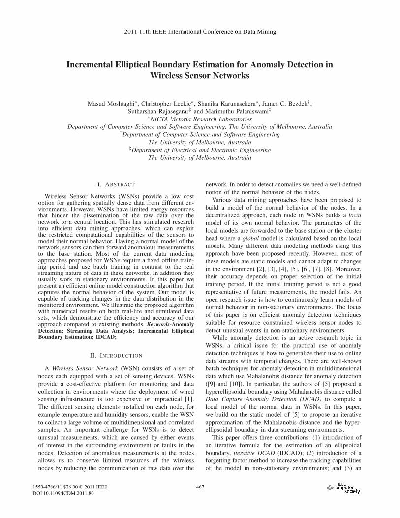
The forgetting factor λ should be close to one. Thesuggested range for λ in the estimation theory literature is[0.9 0.99]. Throughout this paper we use λ = 0.99 and sug-gest that the range for λ for FFIDCAD be [0.99, 0.999]. Thismethod increases the significance of the current measure-ment compared to previous measurements, but for very largek the iterative algorithm becomes unstable. Fig. 2 shows thiseffect on the real-life dataset Grand Saint Bernard (GSB)(see Section VII-A for more details about the GSB dataset).As k →∞ the value in the brackets of (13) approaches I, thus

the characteristic matrix updates approachS−1

kλλ . Therefore, as

k grows large the effects of the new measurement becomes

small andS−1

kλλ controls the change in the characteristic

matrix. As the volume of a hyperellipsoid is proportional to

470

the inverse of the square root of the determinant of its char-acteristic matrix, this update gradually reduces the volumeof the hyperellipsoidal boundary. To deal with this issue, welimit the growth of k by introducing a sliding window basedbenchmark approach and an approximation for it with lowercomputational complexity called the Effective N approach.

0 5000 10000 150000

2000

4000

6000

8000

10000

12000Plot of Eigenvalues of the Characteristic Matrix

GSB Dataset

Samples

Eig

enva

lue

Figure 2. The eigenvalues of the characteristic matrix after each updateusing FFIDCAD. After sample 5000 the larger eigenvalue is very unstable.

A. Benchmark Estimation

To limit the growth of k in the update formulas ofFFIDCAD, we can use FFIDCAD over a sliding windowof size w. To provide a benchmark for comparison werecalculate our overall estimate from the beginning of thewindow to get the exact FFIDCAD ellipsoid after eachinput. This approach is computationally inefficient for anonline algorithm, but it provides the exact value of thehyperellipsoidal boundary using the active measurements,i.e., the measurements in the sliding window, and is used asthe benchmark for comparison of the proposed approach forlimiting the effect of large k in our calculations.

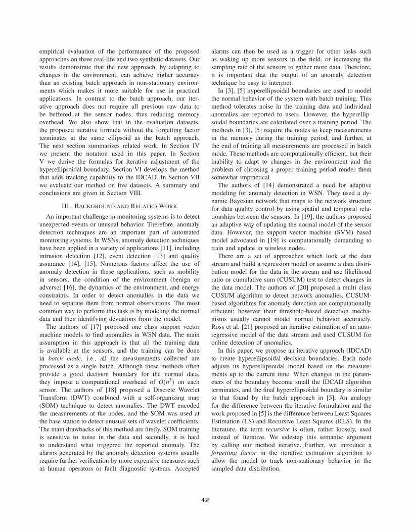
B. Effective N

In this approach, to deal with the issue of large k fortracking, we simply use a constant neff instead of k inEq. 13 when k ≥ neff. The idea is that after k ≥ neff weightsassigned to data samples approach zero, i.e., λ k ∼= 0, sothe corresponding samples have been (almost) forgottencompletely. We suggest neff = 3τ in this paper, whereτ = 1

1−λ is known as the memory horizon of the iterativealgorithm with an exponential forgetting factor λ . A viewof the benchmark and the Effective N tracking approaches isshown in Fig. 3. The boxes show the samples that have beenconsidered in the calculation of the ellipsoidal boundary.In the Effective N approach the weight of older samplesdecreases exponentially, but no cut-off is defined.

kk-n+1k-n-1 k-n k+2k+1k-1……..….

Benchmark: Sliding window of n samples

Time=tk Time=tk+1

kk-n+1k-n-1 k-n k+2k+1k-1……..….

Effective N approach

neff at time=tk

neff at time=tk+1

Discarded samples at tk

Absorbed into

with weight �

1,

−

λkS

0≅effn

λ

Figure 3. A view of the benchmark and the Effective N approaches atsamples k and k +1

VII. EVALUATION

We start this section by introducing the datasets usedin our evaluation of the different methods. Then we showthat IDCAD terminates at the batch approach using all thedatasets. We continue by comparing the proposed EffectiveN approach with the benchmark approach for FFIDCAD.Detection and false alarm rates of the two methods forFFIDCAD on the synthetic datasets are used for comparison.In the synthetic datasets a uniform noise from [−10 10] isadded randomly to 1% of the samples and these samplesare labelled anomalies while the rest are considered normal.Another comparison approach is introduced based on devi-ation from the proposed benchmark approach, which doesnot require a labelled dataset and hence, allows us to usereal-life datasets for comparison. Next, we check the effectsof FFIDCAD on anomaly detection compared to IDCAD.Finally, we compare our proposed FFIDCAD with EffectiveN with a change detection technique proposed in [21].

A. Datasets

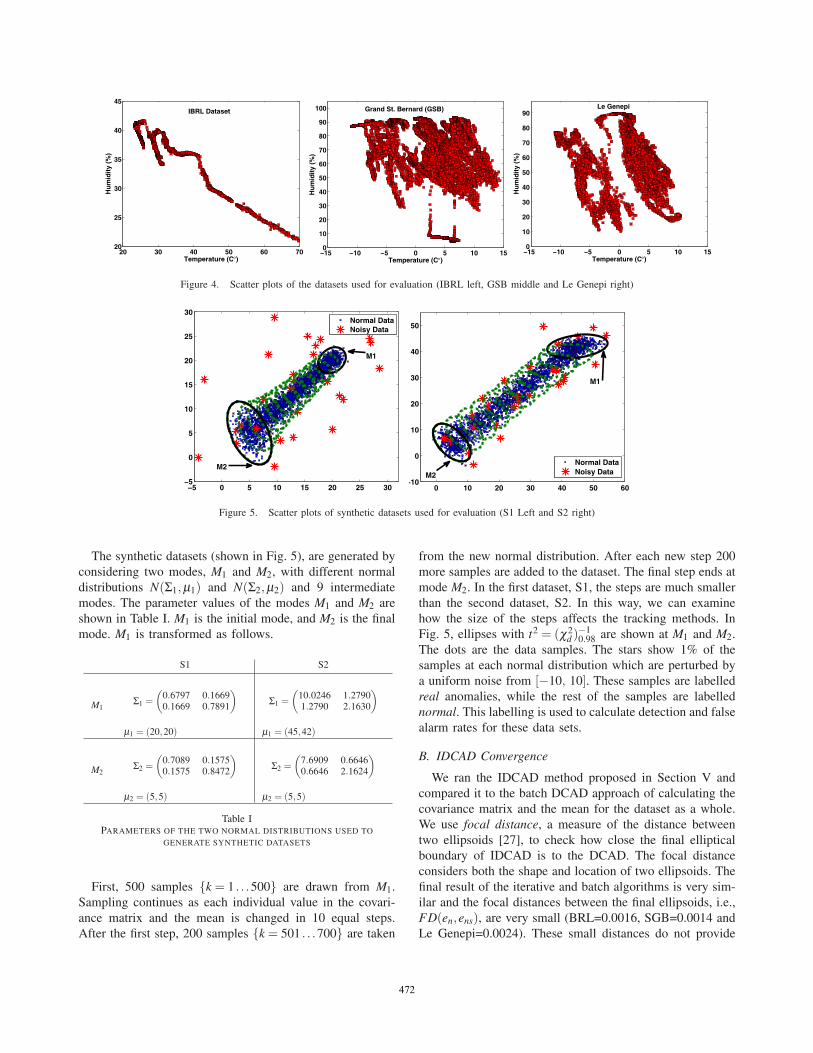
We use three real-life datasets to evaluate our iterativemodel for anomaly detection and compare it with existingmethods. The first dataset (IBRL) consists of measurementscollected by 54 sensors from the Intel Berkeley ResearchLab [25]. In this paper, we used the data from epochs 25000to 30000 of node 18. Fig. 1(a) shows the first 818 samplesin this data. The second dataset (GSB) was gathered in2007 from 23 sensors deployed at the Grand-St-Bernard passbetween Switzerland and Italy [26]. We extracted the datagathered during October by station 10. The third dataset isthe Le Genepi dataset, gathered in 2007 from 16 sensingstations deployed on the rock glacier located at Le Genepiabove Martigny in Switzerland. The data from Station 10 ina twelve days collection period starting at October 10th isused in this paper.

471

20 30 40 50 60 7020

25

30

35

40

45IBRL Dataset

Temperature (C°)

Hu

mid

ity

(%)

−15 −10 −5 0 5 10 150

10

20

30

40

50

60

70

80

90

100 Grand St. Bernard (GSB)

Temperature (C°)

Hu

mid

ity

(%)

−15 −10 −5 0 5 10 150

10

20

30

40

50

60

70

80

90Le Genepi

Temperature (C°)

Hu

mid

ity

(%)

Figure 4. Scatter plots of the datasets used for evaluation (IBRL left, GSB middle and Le Genepi right)

−5 0 5 10 15 20 25 30−5

0

5

10

15

20

25

30

1

1 1

1

2

3

4

5

6

7

8

9

2

3

4

5

6

7

8

9

Normal DataNoisy Data

M1

M2

0 10 20 30 40 50 60−10

0

10

20

30

40

50

1

2

1

5

6

7

8

9

10

1

2

6

7

8

9

10

1112

1

1

1

2

3

4

6

7

2

5

Normal DataNoisy DataM2

M1

Figure 5. Scatter plots of synthetic datasets used for evaluation (S1 Left and S2 right)

The synthetic datasets (shown in Fig. 5), are generated byconsidering two modes, M1 and M2, with different normaldistributions N(Σ1,μ1) and N(Σ2,μ2) and 9 intermediatemodes. The parameter values of the modes M1 and M2 areshown in Table I. M1 is the initial mode, and M2 is the finalmode. M1 is transformed as follows.

S1 S2

M1Σ1 =

(0.6797 0.16690.1669 0.7891

)

μ1 = (20,20)

Σ1 =(

10.0246 1.27901.2790 2.1630

)

μ1 = (45,42)

M2Σ2 =

(0.7089 0.15750.1575 0.8472

)

μ2 = (5,5)

Σ2 =(

7.6909 0.66460.6646 2.1624

)

μ2 = (5,5)

Table IPARAMETERS OF THE TWO NORMAL DISTRIBUTIONS USED TO

GENERATE SYNTHETIC DATASETS

First, 500 samples {k = 1 . . .500} are drawn from M1.Sampling continues as each individual value in the covari-ance matrix and the mean is changed in 10 equal steps.After the first step, 200 samples {k = 501 . . .700} are taken

from the new normal distribution. After each new step 200more samples are added to the dataset. The final step ends atmode M2. In the first dataset, S1, the steps are much smallerthan the second dataset, S2. In this way, we can examinehow the size of the steps affects the tracking methods. InFig. 5, ellipses with t2 = (χ2

d )−10.98 are shown at M1 and M2.

The dots are the data samples. The stars show 1% of thesamples at each normal distribution which are perturbed bya uniform noise from [−10, 10]. These samples are labelledreal anomalies, while the rest of the samples are labellednormal. This labelling is used to calculate detection and falsealarm rates for these data sets.

B. IDCAD Convergence

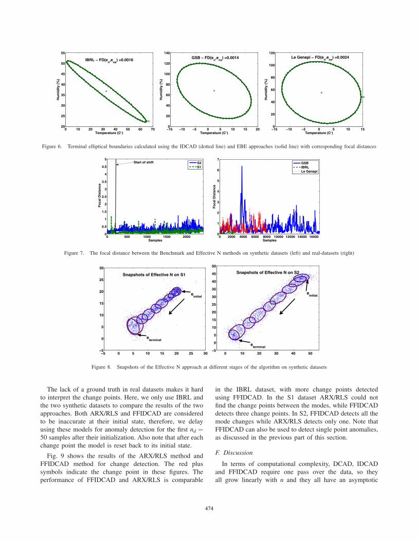
We ran the IDCAD method proposed in Section V andcompared it to the batch DCAD approach of calculating thecovariance matrix and the mean for the dataset as a whole.We use focal distance, a measure of the distance betweentwo ellipsoids [27], to check how close the final ellipticalboundary of IDCAD is to the DCAD. The focal distanceconsiders both the shape and location of two ellipsoids. Thefinal result of the iterative and batch algorithms is very sim-ilar and the focal distances between the final ellipsoids, i.e.,FD(en,ens), are very small (BRL=0.0016, SGB=0.0014 andLe Genepi=0.0024). These small distances do not provide

472

a visually apparent effect on the final boundaries shownin Fig. 6. The dotted-line ellipsoids in Fig. 6 show thefinal ellipsoid obtained from IDCAD and the black solidellipsoids are calculated using the batch approach.

C. Comparison of Tracking

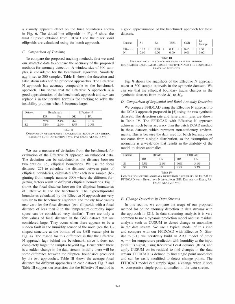
To compare the proposed tracking methods, first we usedour synthetic data to compare the accuracy of the proposedmethods for anomaly detection. A window size of 300 sam-ples is considered for the benchmark algorithm. Similarlyneff is set to 300 samples. Table II shows the detection andfalse alarm rates for the proposed approaches. The EffectiveN approach has accuracy comparable to the benchmarkapproach. This shows that the Effective N approach is agood approximation of the benchmark approach and neff canreplace k in the iterative formula for tracking to solve theinstability problem when k becomes large.

Dataset Benchmark Effective NDR FA DR FA

S1 96% 2.4% 96% 3.1%S2 81% 2.6% 85% 3.3%

Table IICOMPARISON OF DIFFERENT TRACKING METHODS ON SYNTHETIC

DATASETS (DR: DETECTION RATE, FA: FALSE ALARM RATE)

We use a measure of deviation from the benchmark forevaluation of the Effective N approach on unlabeled data.The deviation can be calculated as the distance betweentwo entities, i.e., elliptical boundaries. We use the focaldistance [27] to calculate the distance between pairs ofelliptical boundaries, calculated after each new sample (be-ginning from sample number 300) where the different for-getting factors result in different elliptical boundaries. Fig. 7shows the focal distance between the elliptical boundariesof Effective N and the benchmark. The hyperellipsoidalboundaries calculated by the Effective N approach are verysimilar to the benchmark algorithm and mostly have valuesnear zero for the focal distance (two ellipsoids with a focaldistance of less than 2 in the temperature-humidity inputspace can be considered very similar). There are only afew values of focal distance in the GSB dataset that areconsidered large. They occur when there appears to be asudden fault in the humidity sensor of the node (see the U-shaped structure at the bottom of the GSB scatter plot inFig. 4). The reason for this difference is that the EffectiveN approach lags behind the benchmark, since it does notcompletely forget the samples beyond neff. Hence when thereis a sudden change in the data stream, initially there will besome difference between the elliptical boundaries producedby the two approaches. Table III shows the average focaldistance for different approaches in each dataset. Fig. 7 andTable III support our assertion that the Effective N method is

a good approximation of the benchmark approach for thesedatasets.

Dataset S1 S2 IBRL GSBLeGenepi

EffectiveN

0.13 ±0.00

0.28 ±0.00

0.11 ±0.00

0.65 ±0.01

0.57 ±0.00

Table IIIAVERAGE FOCAL DISTANCE BETWEEN HYPERELLIPSOIDAL

BOUNDARIES CALCULATED USING EFFECTIVE N AND THE BENCHMARK

TRACKING METHODS.

Fig. 8 shows the snapshots of the Effective N approachtaken at 300 sample intervals in the synthetic datasets. Wecan see that the elliptical boundary tracks changes in thesynthetic datasets from mode M1 to M2.

D. Comparison of Sequential and Batch Anomaly Detection

We compare FFIDCAD using the Effective N approach tothe DCAD approach proposed in [5] using the two syntheticdatasets. The detection rate and false alarm rates are shownin Table IV. The FFIDCAD with Effective N approachachieves much better accuracy than the batch DCAD methodin these datasets which represent non-stationary environ-ments. This is because the data used for batch learning doesnot come from a single distribution, so the assumption ofnormality is a weak one that results in the inability of themodel to detect anomalies.

Dataset DCAD FFIDCADDR FA DR FA

S1 55% 2.1% 96% 3.1%S2 29% 1% 85% 3.3%

Table IVCOMPARISON OF THE ANOMALY DETECTION CAPABILITY OF DCAD VS

FFIDCAD WITH EFFECTIVE N APPROACH (DR: DETECTION RATE, FA:FALSE ALARM RATE)

E. Change Detection in Data Streams

In this section, we compare the usage of our proposedmethod for online anomaly detection in data streams withthe approach in [21]. In data streaming analysis it is verycommon to use a dynamic prediction model and use residualanalysis such as CUSUM to detect change or anomaliesin the data stream. We use a typical model of this kindand compare with our FFIDCAD with Effective N. Sim-ilar to [21], we iteratively build an ARX model of ordernp = 4 for temperature prediction with humidity as the input(stimulus signal) using Recursive Least Squares (RLS), andapply CUSUM on its residual to find changes in the datastream. FFIDCAD is defined to find single point anomaliesand can be easily modified to detect change points. TheFFIDCAD model can simply signal a change when it seesna consecutive single point anomalies in the data stream.

473

0 10 20 30 40 50 60 7020

25

30

35

40

45

50

55

IBRL − FD(en,e

ns) =0.0016

800

Temperature (C°)

Hu

mid

ity

(%)

−15 −10 −5 0 5 10 15 200

20

40

60

80

100

120

140GSB − FD(e

n,e

ns) =0.0014

Temperature (C°)

Hu

mid

ity

(%)

−15 −10 −5 0 5 10 150

20

40

60

80

100

120Le Genepi − FD(e

n,e

ns) =0.0024

800

Temperature (C°)

Hu

mid

ity

(%)

Figure 6. Terminal elliptical boundaries calculated using the IDCAD (dotted line) and EBE approaches (solid line) with corresponding focal distances

0 500 1000 1500 20000

0.5

1

1.5

2

2.5

3

3.5

4

4.5

5

Samples

Fo

cal D

ista

nce

S2S1

Start of shift

0 2000 4000 6000 8000 10000 12000 14000 160000

1

2

3

4

5

6

7

Samples

Fo

cal D

ista

nce

GSBIBRLLe Genepi

Figure 7. The focal distance between the Benchmark and Effective N methods on synthetic datasets (left) and real-datasets (right)

−5 0 5 10 15 20 25 30−5

0

5

10

15

20

25

30

Snapshots of Effective N on S1

einitial

eterminal

0 10 20 30 40 50−5

0

5

10

15

20

25

30

35

40

45

50

Snapshots of Effective N on S2

einitial

eterminal

Figure 8. Snapshots of the Effective N approach at different stages of the algorithm on synthetic datasets

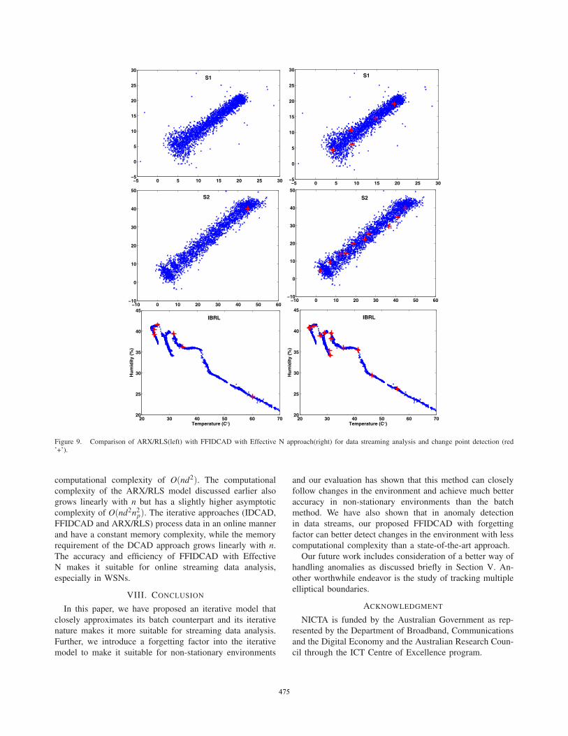
The lack of a ground truth in real datasets makes it hardto interpret the change points. Here, we only use IBRL andthe two synthetic datasets to compare the results of the twoapproaches. Both ARX/RLS and FFIDCAD are consideredto be inaccurate at their initial state, therefore, we delayusing these models for anomaly detection for the first nd =50 samples after their initialization. Also note that after eachchange point the model is reset back to its initial state.

Fig. 9 shows the results of the ARX/RLS method andFFIDCAD method for change detection. The red plussymbols indicate the change point in these figures. Theperformance of FFIDCAD and ARX/RLS is comparable

in the IBRL dataset, with more change points detectedusing FFIDCAD. In the S1 dataset ARX/RLS could notfind the change points between the modes, while FFIDCADdetects three change points. In S2, FFIDCAD detects all themode changes while ARX/RLS detects only one. Note thatFFIDCAD can also be used to detect single point anomalies,as discussed in the previous part of this section.

F. Discussion

In terms of computational complexity, DCAD, IDCADand FFIDCAD require one pass over the data, so theyall grow linearly with n and they all have an asymptotic

474

−5 0 5 10 15 20 25 30−5

0

5

10

15

20

25

30

S1

−5 0 5 10 15 20 25 30−5

0

5

10

15

20

25

30S1

−10 0 10 20 30 40 50 60−10

0

10

20

30

40

50S2

−10 0 10 20 30 40 50 60−10

0

10

20

30

40

50

S2

20 30 40 50 60 7020

25

30

35

40

45

IBRL

Temperature (C°)

Hu

mid

ity

(%)

20 30 40 50 60 7020

25

30

35

40

45

IBRL

Temperature (C°)

Hu

mid

ity

(%)

Figure 9. Comparison of ARX/RLS(left) with FFIDCAD with Effective N approach(right) for data streaming analysis and change point detection (red’+’).

computational complexity of O(nd2). The computationalcomplexity of the ARX/RLS model discussed earlier alsogrows linearly with n but has a slightly higher asymptoticcomplexity of O(nd2n2

p). The iterative approaches (IDCAD,FFIDCAD and ARX/RLS) process data in an online mannerand have a constant memory complexity, while the memoryrequirement of the DCAD approach grows linearly with n.The accuracy and efficiency of FFIDCAD with EffectiveN makes it suitable for online streaming data analysis,especially in WSNs.

VIII. CONCLUSION

In this paper, we have proposed an iterative model thatclosely approximates its batch counterpart and its iterativenature makes it more suitable for streaming data analysis.Further, we introduce a forgetting factor into the iterativemodel to make it suitable for non-stationary environments

and our evaluation has shown that this method can closelyfollow changes in the environment and achieve much betteraccuracy in non-stationary environments than the batchmethod. We have also shown that in anomaly detectionin data streams, our proposed FFIDCAD with forgettingfactor can better detect changes in the environment with lesscomputational complexity than a state-of-the-art approach.

Our future work includes consideration of a better way ofhandling anomalies as discussed briefly in Section V. An-other worthwhile endeavor is the study of tracking multipleelliptical boundaries.

ACKNOWLEDGMENT

NICTA is funded by the Australian Government as rep-resented by the Department of Broadband, Communicationsand the Digital Economy and the Australian Research Coun-cil through the ICT Centre of Excellence program.

475

REFERENCES

[1] A. Willig, “Recent and emerging topics in wireless industrialcommunications: A selection,” IEEE Transactions on Indus-trial Informatics, vol. 4, pp. 102 – 124, 2008.

[2] V. Bhuse and A. Gupta, “Anomaly intrusion detection inwireless sensor networks,” Journal of High Speed Networks,vol. 15, pp. 33–51, 2006.

[3] M. Moshtaghi, S. Rajasegarar, C. Leckie, and S. Karunasek-era, “Anomaly detection by clustering ellipsoids in wirelesssensor networks,” in Fifth International Conference on Intel-ligent Sensors, Sensor Networks and Information Processing(ISSNIP 09), December 2009.

[4] I. Onat and A. Miri, “An intrusion detection system forwireless sensor networks,” in Proc. IEEE International Con-ference on Wireless and Mobile Computing, Networking AndCommunications, August 2005, pp. 253–259.

[5] S. Rajasegarar, J. C. Bezdek, C. Leckie, and M. Palaniswami,“Elliptical anomalies in wireless sensor networks,” ACMTransactions on Sensor Networks (ACM TOSN), vol. 6, no. 1,2009.

[6] S. Rajasegarar, C. Leckie, M. Palaniswami, and J. Bezdek,“Quarter sphere based distributed anomaly detection in wire-less sensor networks,” in Proc. IEEE International Confer-ence on Communication Systems, June 2007, pp. 3864–3869.

[7] S. Rajasegarar, A. Shilton, C. Leckie, R. Kotagiri, andM. Palaniswami, “Distributed training of multiclass conic-segmentation support vector machines on communicationconstrained networks,” in Sixth International Conference onIntelligent Sensors, Sensor Networks and Information Pro-cessing (ISSNIP), December 2010, pp. 211 –216.

[8] B. Sheng, Q. Li, W. Mao, and W. Jin, “Outlier detection insensor networks,” in MobiHoc ’07: Proceedings of the 8thACM International Symposium on Mobile Ad Hoc Networkingand Computing, 2007, pp. 219–228.

[9] V. Hodge and J. Austin, “A survey of outlier detectionmethodologies,” Artif. Intell. Rev., vol. 22, no. 2, pp. 85–126,2004.

[10] S. Rajasegarar, C. Leckie, and M. Palaniswami, “Anomalydetection in wireless sensor networks,” IEEE Wireless Com-munications, vol. 15, no. 4, pp. 34–40, 2008.

[11] V. Chandola, A. Banerjee, and V. Kumar, “Anomaly detection:A survey,” ACM Comput. Surv., vol. 41, pp. 15:1–15:58, July2009.

[12] D. Djenouri, L. Khelladi, and A. Badache, “A survey ofsecurity issues in mobile ad hoc and sensor networks,” IEEEComm. Surveys & Tutorials, vol. 7, no. 4, pp. 2– 28, 2005.

[13] S. Subramaniam, T. Palpanas, D. Papadopoulos, V. Kaloger-aki, and D. Gunopulos, “Online outlier detection in sensordata using nonparametric models,” in 32nd InternationalConference on Very Large Data Bases, September 2006, pp.187–198.

[14] E. W. Dereszynski and T. G. Dietterich, “Spatiotemporalmodels for data-anomaly detection in dynamic environmentalmonitoring campaigns,” ACM Transactions on Sensor Net-works, In Press.

[15] S. Rajasegarar, C. Leckie, and M. Palaniswami, “Detectingdata anomalies in wireless sensor networks,” in Security inAd-hoc and Sensor Networks, July 2009, pp. 231–260.

[16] C. Chong and S. Kumar, “Sensor networks: Evolution, op-portunities, and challenges,” in Proceedings of IEEE, vol. 91,August 2003, pp. 1247–1256.

[17] S. Rajasegarar, C. Leckie, J. Bezdek, and M. Palaniswami,“Centered hyperspherical and hyperellipsoidal one-class sup-port vector machines for anomaly detection in sensor net-works,” IEEE Transactions on Information Forensics andSecurity, vol. 5, no. 3, pp. 518 –533, September 2010.

[18] S. Siripanadorn, W. Hattagam, and N. Teaumroong, “Anomalydetection using self-organizing map and wavelets in wirelesssensor networks,” in Proceedings of the 10th WSEAS Interna-tional Conference on Applied Computer Science, ser. ACS’10,2010, pp. 291–297.

[19] Y. Zhang, N. Meratnia, and P. Havinga, “Adaptive and onlineone-class support vector machine-based outlier detection tech-niques for wireless sensor networks,” International Confer-ence on Advanced Information Networking and ApplicationsWorkshops, vol. 0, pp. 990–995, 2009.

[20] H.-M. Lee and C.-H. Mao, “Finding abnormal events inhome sensor network environment using correlation graph,”in Proceedings of the 2009 IEEE International Conferenceon Systems, Man and Cybernetics. IEEE Press, 2009, pp.1852–1856.

[21] G. J. Ross, D. K. Tasoulis, and N. M. Adams, “Onlineannotation and prediction for regime switching data streams,”in Proceedings of the 2009 ACM Symposium on AppliedComputing. ACM, 2009, pp. 1501–1505.

[22] D. M. Tax and R. P. Duin, “Data description in subspaces,”International Conference on Pattern Recognition, vol. 2, p.2672, 2000.

[23] R. O. Duda, P. E. Hart, and D. G. Stork, Pattern Classification(2nd Edition), 2nd ed. Wiley-Interscience, November 2000.

[24] L. Ljung, System Identification: Theory for the User. PrenticeHall PTR, 1999.

[25] “IBRL-Web,” 2006. [Online]. Available: http://db.lcs.mit.edu/labdata/labdata.html

[26] “SensorScope Web,” 2007. [Online]. Avail-able: http://sensorscope.epfl.ch/index.php/Grand-St-Bernard\Deployment

[27] M. Moshtaghi, T. C. Havens, J. C. Bezdek, L. Park, C. Leckie,S. Rajasegarar, J. M. Keller, and M. Palaniswami, “Clusteringellipses for anomaly detection,” Pattern Recognition, vol. 44,pp. 55–69, January 2011.

476