McCormack | Page 1

Income, weather, and transit dependence: Examining public

transportation ridership in the Chicago Metropolitan Area

Kristen McCormack

April 23, 2015

Pomona College, Claremont, CA

I. Introduction

Weather and Public Transit

In the United States, there is an ongoing debate about the future of public transit systems.

Many factors affect the popularity of public transit, including the quality, price, and convenience

of services, the characteristics of alternatives to services, demographic factors, and cultural

norms. The effects on transit demand of many of these factors, including the price of public

transit, the price of gasoline, service quality and frequency, income, car ownership, and attitudes

towards transit have been studied extensively.

The relationship between weather and public transit ridership, however, has only recently

been explored. Weather is expected to cause changes in transit ridership by affecting the quality

of service, travel time, and experience travelling to and waiting for transit service. The effect of

weather on transit decisions can be characterized by two key behavioral responses. First, people

may substitute one form of transportation for another. For example, if heavy snow increases

traffic congestion or causes roads to seem less safe, people may decide to use public transit

instead of travelling by car. Second, weather may affect ridership by changing the type,

frequency, and timing of discretionary trips. For example, pleasant weather may lead to more

frequent trips to the park while rain may cause cancellations in sporting events or outdoor public

gatherings. People may plan more flexible errands around weather; for example, people may

delay trips to the grocery store if, on a given day, they expect the experience of accessing public

transit to be particularly undesirable. The same type of trip may be more discretionary for some

people than it is for others. For example, some people may have flexible work hours or the

option of working from home while others may face more severe consequences for failing to

appear at their workplace at a designated time.

Previous studies have focused on the relationship between weather and system-wide

public transit ridership. Generally, these studies have observed that adverse weather is correlated

with lower ridership. One study of the relationship between changes in weather and changes in

daily bus and rail ridership in the Chicago area found that warmer temperatures and the existence

of fog led to higher ridership while wind, rain, and snow led to a decrease in ridership; extreme

weather had no significant effect. As expected, the study also found that bus ridership was more

sensitive to weather variation than was rail ridership (Guo et al., 2007). The positive relationship

between temperature and ridership and negative relationship between wind, rain and ridership

was also observed in a study of buses in Gipuzkoa, Spain (Arana et al., 2014). In a study of bus

ridership in Pierce County, Washington, Stover et al. (2012) similarly found that rain, cold

temperatures in winter, snow in fall and winter, and wind in all seasons except summer were

associated with a lower bus ridership. A study of transit choice in Bergen, Norway, found that

wind was the most important variable in explaining travel mode. Generally, however, weather

McCormack | Page 2

was observed to have little effect on decisions to switch between methods of public and private

transportation (Aaheim and Hauge, 2005).

While considerable progress in this area has been made in recent years, there remain

significant gaps in existing literature. Some studies have considered the relationship between

absolute weather conditions and ridership and some have studied the relationship between

relative weather conditions, or changes in conditions from the previous day, and ridership;

however, no studies have considered the effects of both absolute and relative conditions in a

single model. This is concerning because if relative and absolute weather effects are correlated,

models that fail to consider both relative and absolute weather may suffer from omitted-variable

bias. In addition, no studies have compared the effects on ridership of relative and absolute

weather conditions.

Transit Dependence

The effect of transit dependence on the relationship between weather and transit ridership

also remains unexplored. It has been widely observed that the demographic characteristics of a

population affects how that populations uses public transit. In particular, significant differences

have been observed between how people of different levels of income use public transit systems.

Glaeser et al. (2008) suggested that the poor tend to live closer to city centers in order to

have better access to public transit. In the United States, people with low incomes tend to travel

less and take shorter trips than people with higher incomes. While a large proportion of both

low- and high-income populations travels by car, low-income persons are more likely to walk or

bike and are more likely to use bus or rail services than are high-income persons. They are also

more likely to be regular users of public transit (Guiliano, 2005).

Many of these differences may be attributed to lower rates of automobile ownership

among low-income populations. Low-income households are less likely to own a car (Guiliano,

2005) and more likely to share a car among multiple drivers than are high-income households

(Waller, 2005). Lacking access to a car causes lower-income individuals to be more transit

dependent. Their demand for transit is therefore expected to be less responsive to changes in

price or other factors. Indeed, the price elasticity for car owners (-0.41) is more than four times

as large as the price elasticity of non-car owners (-0.10) (Gillen, 1994).

Despite the well-studied differences in transit use by people of different income levels, no

studies have explicitly considered how income may affect the relationship between weather and

transit ridership. Questions concerning transit dependence may be especially important to ask

given the trend over the past century, noted by Garrett & Taylor (1999), in which public transit

ridership has increasingly been comprised of people who are transit dependent due to age,

income, or physical limitations. Over time, public transit systems have been losing market share

to private vehicles, and during this decline, public transit systems have extended services to

wealthier areas rather than improving service for the poor (Garrett & Taylor, 1999). Transit

authorities have received heavy criticism in response to these policies.

Changing Climate

Understanding the relationship between weather and public transit ridership, including

how this relationship is affected by the income of riders and potential riders, is increasingly

important in light of current and future climactic change. Climate change is expected to increase

global mean surface temperatures by 0.3˚C to 4.8˚C by the end of the 21st century (IPCC WG1

McCormack | Page 3

AR5, 2014).1 However, this change is not expected to be uniform across regions or across time.

In addition, climate change will likely increase the variability of weather and frequency and

severity of extreme weather events (Meehl et al., 2000; Greenough et al. 2001; Easterling et al.,

2000). There will likely be fewer days characterized by extreme cold and more days

characterized by extreme heat. In addition, heat waves are expected to occur higher frequently

and to last longer. Precipitation events will also likely occur more frequently and be more

intense. (IPCC WG1 AR5, 2014). Since weather appears to affect ridership and this effect is

likely different for populations of different incomes, gaining a better understanding of how

extreme weather and increased variability in weather will affect ridership may provide insight

into future public transit use.

Policy Relevance

Studying how income affects the relationship between weather and ridership, especially

in a changing climate, is highly relevant to current social, political, and economic debates. A

better understanding of the relationship between weather and transit use may enable improved

transportation system design and superior service provision by transportation authorities. It may

also have significant urban planning and public health implications. For example, understanding

how travel behavior changes in response to extreme weather may inform more targeted

interventions, such as the opening of shelters and public, temperature-controlled buildings in

times of extreme heat or cold. In addition, understanding how different populations may respond

to extreme heat may enable more directed public health warning systems. Therefore, gaining a

better understanding of how extreme weather and increased variability in weather will affect

ridership may enable improved public policy and business practices.

II. Case Study of the Chicago Transit Authority

Overview

This study hopes to addresses the gaps in the weather-transit literature by considering

how income affects the relationship between ridership and absolute and relative weather

conditions. To explore these relationships, the paper focuses on ridership within the Chicago

Transit Authority (CTA) rail system from 2001 to 2013.

Climate of Chicago

The metropolitan area of Chicago is characterized by a continental climate. It has a

significant urban heat island effect that causes the city of Chicago to be warmer than surrounding

areas by, on average, 2°F. The climate of Chicago is also influenced by its proximity to Lake

Michigan, which moderates climate and contributes to high winter precipitation. Weather in

Chicago is highly variable, and Chicago’s location under the polar jet stream causes the area to

experience low-pressure storm systems (Angel, 2009).

Several forms of extreme weather, including heat waves, cold fronts, blizzards, extreme

wind, floods, and tornados affect the Chicago area. Chicago’s most notorious extreme weather

event occurred in the summer of 1995, when a heat wave resulted in 700 heat-related deaths.

1 Temperature projections vary significantly based on future emissions scenarios. Ranges presented in the IPCC

report include the 5% to 95% model ranges. The range represented here includes the ranges from all emission

scenarios.

McCormack | Page 4

People who were isolated and lacked access to transportation were at most risk during this time

(Semanza et al., 1996). The 2012 heat wave, while severe, had much smaller mortality effects.

People, Income, and Transit

In 2013, Chicago was home to 2.7 million people earning a median household income of

$47,270. Nearly a quarter (22.6%) of those people lived below the poverty line. While income

inequality in Chicago ranks it the 8th most unequal city out of the 50 largest cities in the United

States (Berube, 2014), Chicago is not highly segregated by income. Out of the 30 largest

metropolitan areas, Chicago has the 19th highest residential income segregation (Fry and Taylor,

2012).

In 2012, 27.7 percent of households in Chicago do not own a car, ranking Chicago 7th out

of the 30 largest cities in the United States. This percent has also been growing; there was a 2.3

percent decrease in car ownership from 2007 to 2012 (Sivak, 2014).

Chicago Transit Authority

The Chicago Transit Authority (CTA) operates the second largest public transit system in

the United States. The rail system, known as the Chicago ‘L,’ serves 146 stations and the CTA

bus system has over 128 routes (CTA, 2014). Both the rail and the bus systems are the third

largest in the United States by ridership.

The prominence of CTA as a method of transit, the quality of available transit data, and

the variability of weather in Chicago motivated the selection of the CTA for the focus of this

study. In 2007, Guo et al. used system-wide CTA data to observe the effects of changes in

weather on changes in CTA rail and bus ridership. This paper considers both relative and

absolute weather conditions and studies CTA transit system data at the station level, which

allows for the consideration of income differences in the weather-ridership relationship.

III. Data

Sources

Daily station entries for 145 stations were obtained online from the CTA publically

available ridership database.2 Data include daily ‘L’ system ridership by station from January 1,

2001 to December 31, 2013. A review of the ridership data revealed that a noticeable number of

stations were recorded to have 0 riders on a particular day (1.4% of observations). Because this

study does not attempt to capture station closure, these observations were omitted. Observations

with fewer than 20 daily riders were also omitted because the high frequency of these

observations did not appear to reflect true daily ridership (0.3% of observations).

Historic fare data were obtained from the CTA. There were three increases in the base

rail fare over the study period: in 2004 from $1.50 to $1.75, in 2006 to $2.00 and in 2009 to

$2.25. Ultimately, fare information was not used in favor of year fixed effects.

Weather data for the same period from over one hundred stations in the Chicago area

were obtained from the National Oceanic and Atmospheric Administration’s National Climactic

Data Center’s Global Historical Climatology Network (ncdc.noaa.gov). Data include daily totals

for precipitation, snowfall, snow depth, maximum temperature, minimum temperature, average

wind speed, maximum 2-minute and 5-minute wind speeds, among other weather variables. A

dummy variable for fog was calculated from this dataset by combining the data set dummy

2 https://data.cityofchicago.org/Transportation/CTA-Ridership-L-Station-Entries-Daily-Totals

McCormack | Page 5

variables for WT01 (fog, ice fog, or freezing fog), WT02 (heavy fog or heavy freezing fog),

WT21 (ground fog), and WT22 (ice fog or freezing fog).

Demographic data were obtained from the Current Population Survey (CPS) and from the

US Census Bureau. CPS, which is sponsored by the US Census Bureau and the US Bureau of

Labor Statistics, provides nation-wide data related to employment and earnings. For this study,

CPS 5-year data from 2009 to 2013 were used to determine median household income,

unemployment rate, and labor force participation for each census tract in the Chicago area.

Income and employment data were also obtained from 2000 long form Census data on the level

of census tracts. These data were used to linearly interpolate income and employment estimates

for years between 2001 and 2008. Income data were adjusted to 2013 dollars using annual CPI

values for the Chicago-Gary-Kenosha, Ill-Ind-Wisc area (US Department of Labor, Bureau of

Labor Statistics).

Historical gasoline prices were obtained from the U.S. Energy Information

Administration. This dataset includes weekly retail prices for all grades and formulation of

gasoline from 2001 to 2013. Daily values were linearly interpolated from these data. All price

data were adjusted to 2013 dollars using annual CPI values for the Chicago area.

Defining Extreme Weather

To study the effects of weather on ridership, it is necessary to establish definitions for

extreme weather events. Guo et al. (2007) established thresholds to define extreme wind,

temperature, and heavy rain. While a justification for the definition of extreme wind was

provided (“25mph…can blow dust and paper from the ground”), the thresholds provided for

temperature and heavy rain lacked sufficient links to health or safety. The thresholds for

temperature (increase or decrease ≥ 12°F from previous day) appear to be entirely arbitrary. The

threshold for rain similarly lacks support; the threshold was set to the 80th percentile of rainy

days, which corresponds to ≥ 0.6 inches per day, but was not justified further. In addition, an

extreme snow dummy was not included.

Many definitions of extreme heat, rain, snow, and wind have been used in the

meteorological and health literature. To establish the definitions of extreme weather for this

paper, national definitions and local climate deviations were considered. In addition, robustness

checks were performed to test the sensitivity of the model to different definitions of extreme

weather.

Definitions of extreme heat often reference a maximum temperature exceeding a

threshold between 90°F and 100°F (Easterling, 2000; CMAP, 2013). To define extreme heat in

this paper, the 97.5th percentile of maximum temperature over the summer months (June to

August) was determined. This threshold method, when applied to a series of days, has been used

to define a heat wave (Meehl and Tebaldi, 2004). From 2001 to 2013, the 97.5th percentile of

maximum temperatures was 95°F. The National Weather Service typically issues warnings for

extreme heat based on the Heat Index, which is determined both by temperature and by relative

humidity. Excessive heat warnings are issued if a heat index of 105°F persists for more than

three hours or if a heat index of 115°F is ever observed. For all relative humidity levels within a

normal range, a 95°F temperature corresponds to warnings for at least extreme caution, and

potentially danger or extreme danger of heat disorders with “prolonged exposure or strenuous

activity.” A temperature of 100°F, which was used to test the sensitivity of this threshold,

corresponds to danger or extreme danger for all levels of relative humidity.

McCormack | Page 6

Extreme cold is defined by the city of Chicago as days where the minimum temperature

falls below 32°F. Because most travel takes place during the day, the definition provided by

Easterling (2000) was considered. By this definition, days characterized by extreme cold are

those in which the maximum temperature fell below freezing. In Chicago’s winter months

(December to February), however, more than 40% of days fit this definition. Therefore, this

study took an approach similar to that of Medina-Ramon et al. (2006) and tested the model with

definitions extreme cold as the 1st (10°F) and 5th (17°F) percentiles of maximum temperature in

the winter months. The initial test was conducted with extreme cold defined as 15°F, which falls

between these definitions.

Since plowing roads and diverting water can greatly affect the impact of precipitation on

a population, precipitation may be considered to be more dependent on city-specific

infrastructure than is extreme temperature. Therefore, several definitions of extreme rain and

snow were also used. Days with heavy rain were defined as those with greater than 0.6in (81st

percentile of rainy days). Extreme rain was not found to be significant in the model for a 0.6in

cutoff or for a 2in cutoff (99th percentile of rainy days). Days with heavy snow were defined as

those with snowfall greater than 2in (76th percentile of snowy days). To test the sensitivity of the

model to this threshold, a 3in (88th percentile of snowy days) threshold was also considered.

Days with extreme wind were defined as those with a greater than 25mph maximum 2-

minute wind speed (Guo et al., 2007).

Geographic Analysis

For this analysis, median household income, labor force participation, and the

unemployment rate were estimated for the population entering each transit station. People may

walk, bike, or take other forms of public transit to a transit station. Ideally, it would be possible

to capture both those who walk to the metro and those who take a combination of bus and transit

to their destination, but the current data availability would make such an analysis unfeasible.

Therefore, estimates of the demographics of those entering each station were calculated based on

the characteristics of the surrounding community, which was defined as those living within a

ring of a defined radius around each station.

Several studies have estimated the distance that people are willing to walk to access

public transit. Estimates for how far the average person is willing to walk to public transit

typically fall close to 0.4 km (Zhao et al., 2007). In a study of the Toronto Transit Commission,

Alshalalfah and Shalaby (2007) found that 60% of transit users lived within 0.3km airline

distance of a transit station. O’Sullivan and Morrall (1996) found that in Calgary, Canada, people

typically walk farther to train stations than to bus stops and the average walking distance to

stations was 0.6km in the suburbs and 0.3km in the city. The 75th percentile walking distance to

stations was 0.8km in the suburbs and 0.4km in the city.

For this study, yearly census tract data and 0.4km and 1km buffer zones were used to

estimate the demographic characteristics of each station. Using ArcGIS, intersections of these

buffer zones and census tracts were created. Labor force participation, unemployment rate, and

median household income of each buffer zone were then determined assuming uniform

population density across each census tract. Illustrations of how these buffer zones were used to

represent different income levels and different levels of transit ridership is provided in the

appendix.

McCormack | Page 7

Summary Statistics

The following variables were used in this analysis. Summary statistics for per-station

daily ridership, median household income, the unemployment rate, and the size of the labor force

were calculated by determining the average characteristics of the population living within 0.4km

of each station for every day in the study period. Summary statistics for weather and prices are

calculated over the time period of the study.

Table 1: Summary Statistics (0.4km, N=664,615)

Variable Mean Std. Dev Min Max

Daily riders per station 3,155.985 3,003.337 20 36,017

Median household income (2013 dollars) 57,991.61 25,228.52 13,234.58 128,292.4

Unemployment rate (%) 10.685 7.824 1.149 63.664

Size of labor force 1,914.66 1,419.825 155.436 8,010.312

Maximum temperature (°F) 59.544 21.138 -0.94 102.92

Daily precipitation (inches) 0.104 0.325 0 6.858

Daily snowfall (inches) 0.102 0.616 0 13.583

Fastest 2-minute wind speed (mph) 19.542 5.864 6.935 55.029

Retail price of gasoline (2013 dollars/gallon) 2.944 0.816 1.390 4.588

IV. Theoretical Framework

As noted by Guo et al. (2007), ridership can be modeled using two main methods. First, it

may be modeled in absolute terms as the number of riders who entered the system during a given

day. Alternatively, it may be measured as the number of riders who entered the system relative to

ridership from the previous day or from previous months. The second method, which has been

favored by Guo et al. (2007) allows the model to capture short-term behavioral changes

associated with weather but does not capture the impact of absolute weather conditions.

However, the method of measuring absolute weather conditions is problematic because it may be

influenced by seasonal factors unrelated to weather. In addition, other variables influencing

ridership must be included in absolute models because they may study changes over period of

time in which changes in factors, such as price and population, may affect ridership. The

challenge of using absolute models can be mitigated somewhat by creating separate models for

each season (Stover & McCormack, 2012).

In this paper, I present a hybrid approach, which measures absolute ridership as a

function of absolute weather and changes in weather from the previous day. This model therefore

captures both the effect of absolute weather on ridership and the effect of relative weather on

ridership. An individual may make a transit decision based on absolute weather (“It is cold

outside”), previous weather (“It is warmer than it has been), and future weather forecasts (“It is

expected to be warmer tomorrow”). Because expectations of future weather are more difficult to

determine, only absolute weather and changes in weather conditions from the previous day were

included in this analysis.

To study the effect of income on the relationship between weather and ridership, separate

models were also created for income brackets divided along several different income levels.

McCormack | Page 8

Different thresholds, including the 20th, 50th, and 70th percentiles of income were used to test the

sensitivity of these divisions. This analysis attempts to consider the behavioral changes of people

who are dependent on transit because of income, so a division between those with very low

income, defined as those with income lower than the bottom 10th percentile of income, was also

included in this analysis.

To prevent bias in the coefficients, other variables unrelated to weather that affect

ridership were included (Stover & McCormack, 2012). These variables capture the price of

alternatives to transit (price of gasoline), number of workers (size of labor force, unemployment),

as well as time and place (day of the week, station/route). Month fixed effects were included to

account for seasonal variation in ridership. In favor of including a variable for the price of transit

(fare), year fixed effects were also included. These fixed effects, which entirely capture fare

changes, also control for changes in unobserved factors affecting transit over time.

The theoretical model presented in this paper is as follows (i=station-day):

𝑟𝑖𝑑𝑒𝑟𝑠𝑖 = 𝛽0 + (𝛽1𝑔𝑎𝑠𝑝𝑟𝑖𝑐𝑒 + 𝛽2𝑓𝑎𝑟𝑒) + (𝛽3𝑙𝑎𝑏𝑜𝑟𝐹𝑜𝑟𝑐𝑒 + 𝛽4𝑢𝑛𝑒𝑚𝑝𝑅𝑎𝑡𝑒) + (𝛽𝑖𝑤𝑒𝑎𝑡ℎ𝑒𝑟 + 𝛽𝑗Δ𝑤𝑒𝑎𝑡ℎ𝑒𝑟 +

𝛽𝑘𝑒𝑥𝑡𝑟𝑒𝑚𝑒𝑊𝑒𝑎𝑡ℎ𝑒𝑟) + (𝛽𝑙𝑑𝑎𝑦𝑇𝑦𝑝𝑒 + 𝛽𝑚𝑚𝑜𝑛𝑡ℎ𝐷𝑢𝑚𝑚𝑖𝑒𝑠 + 𝛽𝑚𝑦𝑒𝑎𝑟𝐷𝑢𝑚𝑚𝑖𝑒𝑠 + 𝛽𝑚𝑠𝑡𝑎𝑡𝑖𝑜𝑛𝐷𝑢𝑚𝑚𝑖𝑒𝑠) + 𝜀𝑛

V. Methodological Approach

To develop and evaluate a model of transit ridership, the hybrid model proposed in this

paper was tested. Initially, the model was designed to include only non-weather variables.

Weather variables and change in weather variables were added incrementally to this basic, non-

weather model, so that the effect of the addition of each set of variables could be observed.

Absolute weather was included, followed by extreme weather and finally changes in weather

from the previous day.

After this testing, the model was then estimated for populations of different income

levels. The difference in the value and significance of coefficients between these groups was

observed.

VI. Fitting the Model

Model Specifications

Table 2 depicts various model specifications. In the original model (Model 1), non-

weather, non-income explanatory variables were included. In Models 2, 3, and 4, basic absolute

weather, extreme weather, and relative weather were added. In Model 5, extreme wind and rain

were excluded. Because 0.4km buffer zones have the greatest theoretical basis, they were used in

specifying the model. Once the final model was selected (Model 5), model coefficients were

estimated with 1km data. There were very few differences between the 0.4km and 1km models.

In addition, the same variables that were not significant at the 1% level when tested with 0.4km

data were also not significant when tested with the 1km data. Due to the results of a Breush-

Pagen/Cook-Weisberg test, which suggested evidence of heteroskedasticity, robust standard

errors were used in all model estimations.

The selected model (Model 5) reveals that higher ridership is associated with a higher

price of gas and a larger labor force. The relationship between the unemployment rate and

ridership was not significant. However, because only a few fare changes occurred during the

McCormack | Page 9

study period, this coefficient estimate may have little meaning. Robustness checks for the

thresholds of extreme weather were conducted and are included in the appendix.

VI. Results

Model of Ridership for All Income Levels

Ridership is expected to be higher on warmer days with less rain, snow, and wind. An

increase in temperature of 10°F, for example, would, on average, be correlated with an increase

in per station daily ridership of about 50 riders. An increase in rain and snow by 1 inch is

correlated with, on average, a decrease in per station ridership of 65 and 44 riders respectively.

An increase in 2-minute maximum wind speeds of 5mph is associated with 21 fewer riders. The

absolute effects of non-extreme weather on ridership, while not insignificant, do appear to be

small. Given an average daily per-station ridership of 3,156 each of these effects would account

for approximately a 1 to 2 percent change in ridership. The relationship between fog and

ridership is not significant.

Extreme heat and cold are associated with lower ridership, but extreme snow is

associated with higher ridership. Days with extreme heat and cold are associated with about 139

and 169 fewer riders, on average. Days with extreme snow are associated with 146 more riders,

on average. These results should be interpreted as a non-continuous shift in the linearly modeled

relationship between absolute weather conditions and ridership. For example, a day where the

maximum temperature is 10°F would be expected to have, on average, (20 × 5) + 169 = 269

fewer riders than a day when the maximum temperature reaches 30°F.

The interpretation of the relative weather coefficients is less intuitive than is the

interpretation of absolute and extreme weather effects. Ridership is expected to be higher when

the current day is cooler, snowier, windier, and foggier than the previous day. The relationship

between ridership and changes in rain from the previous day was not significant.

Model of Ridership for People of Different Incomes

To determine whether the ridership behavior of stations of different income levels follow

the same or different models, a Chow test was conducted for several income divisions using

Model 5. Once again, 0.4km data were used. Stations were divided into two groups based on the

10th ($27,804), 20th ($32,390), 50th ($54,222), and 70th ($73,330) percentiles of household

income. In all of these divisions, the null hypothesis was rejected at the 1% level indicating that

there is strong evidence that there is a different relationship between ridership and the

explanatory variables for low- and high-income stations.

To examine the differences between the two groups, Model 5 was estimated for low- and

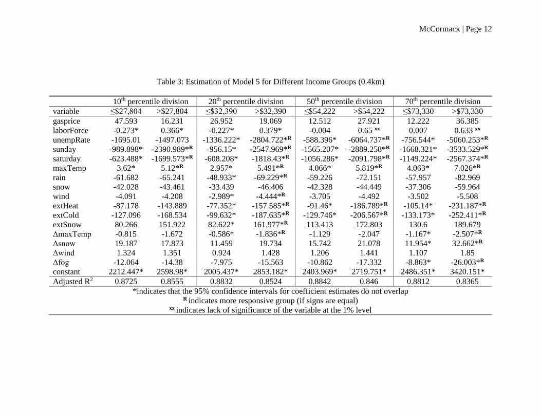
high- income groups of stations. The coefficient estimates for these different groups appear in

Table 3. Without exception, when differences between higher income and lower income models

are significant at the 1% level, ridership at lower-income stations is less sensitive to the

explanatory variable than is ridership at higher-income stations.

Higher income station ridership appears to be more sensitive to both non-weather related

and weather-related factors. Across income divisions, higher income station ridership is

consistently more responsive to the day of the week. In three of four divisions, higher income

stations were more responsive to the unemployment rate.

Across income divisions, higher income station ridership is consistently more sensitive to

temperature. In three out of four divisions, higher income stations appear to be more responsive

McCormack | Page 10

to extreme heat and extreme cold. In half of the income divisions, higher-income stations appear

to more sensitive to a change in temperature from the previous day. When income was divided at

the 20th percentile, ridership at higher-income stations appeared to additionally be more

responsive than lower-income stations to rain, wind, and extreme snow. When income was

divided at the 70th percentile, ridership at higher-income stations was also more responsive to

changes in snow and fog.

Model of Ridership for People of Different Incomes: Accounting for Size

There is a noticeable difference in the number of people per day that enter low- and high-

income stations. This difference is illustrated in the two maps of income and ridership that are

included in the Appendix. Stations closer to the city center tend to have a greater number of

riders and tend to be in areas with higher median income. It is important to note, therefore, that

while the coefficient differences illustrated in Table 3 demonstrate that high-income station

ridership is more responsive to explanatory variables than is the station ridership of low income

stations, it does not necessarily follow that high-income individuals are more responsive to these

factors than are low-income individuals. Indeed, when coefficients are normalized by average

per-day station ridership, as seen in Table 5, the rich appear to be more responsive than the poor

only to the day of the week and, in half of the income divisions, to the unemployment rate.

By contrast, the poor appear to be more responsive than the rich in several ways, all of

which only appear for the 10th and 20th percentile divisions. In these two divisions, the poor

appear to be more responsive to the price of gas and to the size of the labor force than are the

rich. In the 10th percentile division, they also appear to be more responsive to the unemployment

rate. The poor are also more responsive to temperature, rain, and wind in these divisions. In the

10th percentile division, they are also more responsive to snow.

Possible interpretations of these results follow in the conclusion.

McCormack | Page 11

Table 2: Comparison of Regressions (0.4km)

variable Model 1 Model 2 Model 3 Model 4 Model 5 Model 5 (1km)

gasprice 35.757 24.984 22.592 19.554 20.004 20.170

laborForce 0.376 0.376 0.376 0.376 0.376 0.153

unempRate -1461.823 -1459.592 -1459.734 -1459.617 -1459.523 -2135.903

sunday -2243.704 -2246.861 -2247.462 -2246.647 -2246.585 -2245.178

saturday -1590.710 -1589.218 -1589.591 -1588.811 -1588.589 -1587.155

maxTemp - 4.828 4.648 4.970 4.957 4.949

rain - -64.947 -56.458 -49.185 -65.453 -65.613

snow - -2.268 xx -29.164 -44.726 -44.185 -44.171

wind - -3.145 -2.405 -3.890 -4.155 -4.144

fog - -2.879 xx -5.436 xx 3.392 xx - -

extHeat - - -143.928 -139.449 -139.363 -139.355

extCold - - -163.452 -166.787 -168.744 -168.847

extRain - - -18.369 xx -17.593 xx - -

extSnow - - 145.986 143.650 146.110 145.794

extWind - - -9.137 xx -7.833 xx - -

ΔmaxTemp - - - -1.527 -1.566 -1.561

Δrain - - - -9.361 xx - -

Δsnow - - - 19.282 18.476 18.516

Δwind - - - 1.454 1.349 1.346

Δfog - - - -15.217 -14.419 -14.396

Constant (Jan, 2001) 2520.096 2450.616 2458.545 2479.431 2485.796 1585.988

Adjusted R2 0.8553 0.8556 0.8557 0.8557 0.8557 0.8564

all unmarked coefficients are significant at the 1% level

xx indicates lack of significance at the 1% level

McCormack | Page 12

Table 3: Estimation of Model 5 for Different Income Groups (0.4km)

10th percentile division 20th percentile division 50th percentile division 70th percentile division

variable ≤$27,804 >$27,804 ≤$32,390 >$32,390 ≤$54,222 >$54,222 ≤$73,330 >$73,330

gasprice 47.593 16.231 26.952 19.069 12.512 27.921 12.222 36.385

laborForce -0.273* 0.366* -0.227* 0.379* -0.004 0.65 xx 0.007 0.633 xx

unempRate -1695.01 -1497.073 -1336.222* -2804.722*R -588.396* -6064.737*R -756.544* -5060.253*R

sunday -989.898* -2390.989*R -956.15* -2547.969*R -1565.207* -2889.258*R -1668.321* -3533.529*R

saturday -623.488* -1699.573*R -608.208* -1818.43*R -1056.286* -2091.798*R -1149.224* -2567.374*R

maxTemp 3.62* 5.12*R 2.957* 5.491*R 4.066* 5.819*R 4.063* 7.026*R

rain -61.682 -65.241 -48.933* -69.229*R -59.226 -72.151 -57.957 -82.969

snow -42.028 -43.461 -33.439 -46.406 -42.328 -44.449 -37.306 -59.964

wind -4.091 -4.208 -2.989* -4.444*R -3.705 -4.492 -3.502 -5.508

extHeat -87.178 -143.889 -77.352* -157.585*R -91.46* -186.789*R -105.14* -231.187*R

extCold -127.096 -168.534 -99.632* -187.635*R -129.746* -206.567*R -133.173* -252.411*R

extSnow 80.266 151.922 82.622* 161.977*R 113.413 172.803 130.6 189.679

ΔmaxTemp -0.815 -1.672 -0.586* -1.836*R -1.129 -2.047 -1.167* -2.507*R

Δsnow 19.187 17.873 11.459 19.734 15.742 21.078 11.954* 32.662*R

Δwind 1.324 1.351 0.924 1.428 1.206 1.441 1.107 1.85

Δfog -12.064 -14.38 -7.975 -15.563 -10.862 -17.332 -8.863* -26.003*R

constant 2212.447* 2598.98* 2005.437* 2853.182* 2403.969* 2719.751* 2486.351* 3420.151*

Adjusted R2 0.8725 0.8555 0.8832 0.8524 0.8842 0.846 0.8812 0.8365

*indicates that the 95% confidence intervals for coefficient estimates do not overlap R indicates more responsive group (if signs are equal)

xx indicates lack of significance of the variable at the 1% level

McCormack | Page 13

Table 4: Estimation of Model 5 for Different Income Groups by Percent of Average Ridership (0.4km)

10th percentile division 20th percentile division 50th percentile division 70th percentile division

variable ≤$27,804 >$27,804 ≤$32,390 >$32,390 ≤$54,222 >$54,222 ≤$73,330 >$73,330

gasprice 47.593* R 16.231* 26.952* R 19.069* 12.512 27.921 12.222 36.385

laborForce -0.273* R 0.366* -0.227* R 0.379* -0.004 0.65 xx 0.007 0.633 xx

unempRate -1695.01* R -1497.073* -1336.222 -2804.722 -588.396* -6064.737*R -756.544* -5060.253*R

sunday -989.898* -2390.989*R -956.15* -2547.969*R -1565.207* -2889.258*R -1668.321* -3533.529*R

saturday -623.488* -1699.573*R -608.208* -1818.43*R -1056.286* -2091.798*R -1149.224* -2567.374*R

maxTemp 3.62* R 5.12 2.957* R 5.491* 4.066 5.819 4.063 7.026

rain -61.682* R -65.241 -48.933* R -69.229* -59.226 -72.151 -57.957 -82.969

snow -42.028* R -43.461 -33.439 -46.406 -42.328 -44.449 -37.306 -59.964

wind -4.091* R -4.208 -2.989* R -4.444* -3.705 -4.492 -3.502 -5.508

extHeat -87.178 -143.889 -77.352 -157.585 -91.46 -186.789 -105.14 -231.187

extCold -127.096 -168.534 -99.632 -187.635 -129.746 -206.567 -133.173 -252.411

extSnow 80.266 151.922 82.622 161.977 113.413 172.803 130.6 189.679

ΔmaxTemp -0.815 -1.672 -0.586 -1.836 -1.129 -2.047 -1.167 -2.507

Δsnow 19.187 17.873 11.459 19.734 15.742 21.078 11.954 32.662

Δwind 1.324 1.351 0.924 1.428 1.206 1.441 1.107 1.85

Δfog -12.064 -14.38 -7.975 -15.563 -10.862 -17.332 -8.863 -26.003

constant 2212.447* 2598.98* 2005.437* 2853.182* 2403.969* 2719.751* 2486.351 3420.151

avg riders 1705.861 3317.96 1545.986 3557.747 2370.929 3936.327 2434.915 4833.531

Adjusted R2 0.8725 0.8555 0.8832 0.8524 0.8842 0.846 0.8812 0.8365

*indicates that the 95% confidence intervals for coefficient estimates do not overlap R indicates more responsive group (if signs are equal)

xx indicates lack of significance of the variable at the 1% level

McCormack | Page 14

VIII. Conclusion

Relationship between Ridership and Weather

The general model presented in this paper reveals results consistent with the majority of

literature. As temperature increases, there is an increase in ridership, but this effect is very small.

Days with more rain, snow, fog, and wind are associated with a decrease in ridership. Extreme

heat and cold are associated with a decrease in ridership while extreme snow was associated with

an increase in ridership. This may be because extreme snow makes driving conditions unsafe.

When incorporated into a model that also examines absolute weather, the effects of

relative weather on ridership change from those observed by Guo et al. (2007). While Guo found

that an increase in ridership was associated with an increase in temperature from the previous

day and a decrease in precipitation and wind, this model finds that an increase in ridership is

associated with a decrease in temperature and rain and an increase in snow and wind.

Transit Dependence

Without exception, ridership at high-income stations appears to be more responsive to

model parameters than was ridership at lower-income stations. However, when results are

adjusted by average per-station ridership of stations in each grouping, it appears that while

station ridership in rich neighborhoods may be more responsive in absolute terms to the

explanatory variables, a greater percent of potential high-income riders do not appear to be

deterred from or attracted to subway ridership as a result of weather conditions.

Indeed, when coefficient estimates are adjusted by the average per-station ridership of

stations in each income group, it appears that the rich are, by and large not more responsive than

the poor; the rich are only consistently more responsive than the poor to the fixed effect

representing the weekends and holidays. Their ridership may decline more than the ridership of

the poor during weekends because they may work less than the poor on weekends. Alternatively,

stations in rich neighborhoods may correspond to stations in areas where many people of both

low- and high-incomes work.

The results of this analysis suggest that very low-income groups may actually be more

responsive than higher-income groups to weather conditions. For the 10th and 20th percentile

divisions, the poor appear to be more responsive to the price of gasoline, the size of the labor

force, and, for the 10th percentile division, the unemployment rate. The poor also appear to be

more responsive to temperature, rain, wind, and in the 10th percentile division, snow.

This finding does not appear to be consistent with the notion of transit dependence. Since

lower income groups have poorer access to alternative forms of transit, it may be expected that

they will be less responsive to changes in weather.

Several alternative explanations may shed light on this trend. First, the poor may walk

greater distances or take more forms of transit to and from the metro than do the rich. They

therefore may be exposed to weather conditions for a longer period of time than are the rich. The

greater responsiveness of the poor to weather may also be related to the commonly observed

trend that lower-income neighborhoods tend to have poorer infrastructure and public services

than do higher-income neighborhoods (Inman & Rubinfeld, 1979). If the streets of rich

neighborhoods are plowed before the streets of lower-income neighborhoods, high-income

persons may be able to access the metro when doing so remains unfeasible for low-income

persons.

McCormack | Page 15

It is important to note that, while the correspondence of high-income stations with

downtown business districts may explain the greater responsiveness of ridership at high-income

stations to the day of the week, this trend is unlikely to explain the apparent greater

responsiveness of ridership at very low-income stations to temperature, rain, snow and wind. The

majority of stations in the downtown area, as illustrated by the map in the appendix, have a

median household income greater than $100,000. If observed responsiveness were driven by this

trend, significant differences in responsiveness would likely appear in the higher income

divisions, such as the 50th percentile division, where the sample sizes of the two groups are more

even and income divisions correspond more clearly to division between downtown and not-

downtown locations.

While neither the poor nor the rich appear to be more responsive to extreme weather, it is

important to note that, due to the limited number of days with extreme weather, the confidence

intervals around all coefficient estimates were large. For the two lowest percentile divisions, the

poor did appear to be more responsive to these events than the rich, although not significantly so.

Policy Implications

The general model presented in this paper provides evidence for the hypothesis that

public transit ridership is affected by absolute, relative, and extreme weather. People respond

most dramatically to extreme heat, cold, and snow and they have moderate responses to rain,

snow, and temperature. Ridership appears to respond to a lesser extent to wind and changes in

weather from the previous day.

As the climate warms, we may expect to see a greater frequency of warm days and days

characterized by extreme heat, and we may expect fewer days to be characterized by extreme

cold. As more becomes known about the future of climate in the Chicago area and in other cities,

models such as those presented in this paper may be used to enable better service provision and

design of public transit systems.

The comparison of high- and low-income stations reveals a surprising trend: the lowest-

income populations, those who would be expected to be most transit-dependent, are more

responsive to absolute weather than are high-income populations. This paper offers several

potential explanations for this trend. Lower-income individuals may be more exposed to weather

conditions when travelling to and from the metro system, and lower-income neighborhoods may

receive inferior public services that make accessing the metro system difficult.

If the most-transit dependent populations have trouble accessing transportation during

adverse weather conditions, this may raise several concerns. First, lack of mobility has been

widely understood to be a risk-factor in extreme heat events (Semanza et al., 1996). In addition,

this trend is concerning because, if those persons who are most dependent on public transit are

the least able to adapt to changes in weather, it may be possible that the lack of sufficient public

services to low-income neighborhoods or the lack of sufficient transportation to metro stations is

deterring low-income persons from make trips that are important for employment, health, or

general quality of life. This trend therefore merits more extensive exploration.

McCormack | Page 16

VIII. References

Aaheim, H. A., & Hauge, K. E. (2005). Impacts of climate change on travel habits: A national

assessment based on individual choices. Retrieved from

http://brage.bibsys.no/xmlui/handle/11250/191992

Alshalalfah, B. W., & Shalaby, A. S. (2007). Case study: Relationship of walk access distance to

transit with service, travel, and personal characteristics. Journal of Urban Planning and

Development, 133(2), 114-118.

Angel, J. (2009). Climate of Chicago-Description and normals [Prairie Research Institute].

Retrieved February 14, 2015, from

http://www.sws.uiuc.edu/atmos/statecli/General/chicago-climate-narrative.htm

Arana, P., Cabezudo, S., & Peñalba, M. (2014). Influence of weather conditions on transit

ridership: A statistical study using data from Smartcards. Transportation Research Part A:

Policy and Practice, 59, 1–12. doi:10.1016/j.tra.2013.10.019

Berube, A. (2014). All cities are not created unequal. Brookings Institution, Metropolitan

Opportunity Series, 51.

Chicago Metropolitan Agency for Planning (2013). Appendix A: Primary impacts of climate

change in the Chicago region.

Chicago Transit Authority facts at a glance. (Spring 2014). Retrieved February 15, 2015, from

http://www.transitchicago.com/about/facts.aspx

Easterling, D. R., Meehl, G. A., Parmesan, C., Changnon, S. A., Karl, T. R., & Mearns, L. O.

(2000). Climate extremes: observations, modeling, and impacts. Science, 289(5487), 2068-

2074.

Garrett, M., & Taylor, B. (1999). Reconsidering social equity in public transit. Berkeley

Planning Journal, 13(1). Retrieved from http://escholarship.org/uc/item/1mc9t108

Gillen, D. (1994). Peak pricing strategies in transporation, utilities, and tele-communications:

Lessons for road pricing. Curbing Gridlock. Trnsportaiton Research Board: 115-151.

Glaeser, E. L., Kahn, M. E., & Rappaport, J. (2008). Why do the poor live in cities? The role of

public transportation. Journal of Urban Economics, 63(1), 1–24.

doi:10.1016/j.jue.2006.12.004

Greenough, G., McGeehin, M., Bernard, S. M., Trtanj, J., Riad, J., & Engelberg, D. (2001). The

potential impacts of climate variability and change on health impacts of extreme weather

events in the United States. Environmental Health Perspectives, 109(Suppl 2), 191-198.

Giuliano, G. (2005). Low income, public transit, and mobility. Transportation Research Record:

Journal of the Transportation Research Board, 1927(1), 63-70.

Guo, Z., Wilson, N., & Rahbee, A. (2007). Impact of weather on transit ridership in Chicago,

Illinois. Transportation Research Record: Journal of the Transportation Research Board,

2034, 3–10. doi:10.3141/2034-01

Inman, R. & Rubinfeld, D. (1979). The judicial pursuit of local fiscal equity, Harvard Law

Review, 92, 1662-1750.

Intergovernmental Panel on Climate Change (IPCC) (2014), Climate Change 2014: Synthesis

Report. Contribution of Working Groups I, II and III to the Fifth Assessment Report of the

Intergovernmental Panel on Climate Change [Core Writing Team, R.K. Pachauri and L.A.

Meyer (eds.)]. IPCC, Geneva, Switzerland, 151 pp.

Medina-Ramón, M., Zanobetti, A., Cavanagh, D. P., & Schwartz, J. (2006). Extreme

temperatures and mortality: assessing effect modification by personal characteristics and

McCormack | Page 17

specific cause of death in a multi-city case-only analysis. Environmental health

perspectives, 1331-1336.

Meehl, G. A., & Tebaldi, C. (2004). More intense, more frequent, and longer lasting heat waves

in the 21st century. Science, 305(5686), 994-997.

Meehl, G. A., Zwiers, F., Evans, J., Knutson, T., Mearns, L., & Whetton, P. (2000). Trends in

extreme weather and climate events: Issues related to modeling extremes in projections of

future climate change. Bulletin of the American Meteorological Society, 81(3), 427–436.

doi:10.1175/1520-0477(2000)081<0427:TIEWAC>2.3.CO;2

O'Sullivan, S., & Morrall, J. (1996). Walking distances to and from light-rail transit stations.

Transportation Research Record: Journal of the Transportation Research Board, 1538(1),

19-26.

Fry, R. & Taylor, P. (2012). The rise of residential segregation by income. Pew Research Center.

Social and Demographic Trends.

Semenza, J. C., Rubin, C. H., Falter, K. H., Selanikio, J. D., Flanders, W. D., Howe, H. L., &

Wilhelm, J. L. (1996). Heat-related deaths during the July 1995 heat wave in Chicago. New

England Journal of Medicine, 335(2), 84–90. doi:10.1056/NEJM199607113350203

Sivak, M. (2014). Has motorization in the US Peaked? Part 4: Households without a light-duty

vehicle. University of Michigan Transportation Research Institute. No. UMTRI-2014-5.

Stover, V. W., & McCormack, E. D. (2012). The impact of weather on bus ridership in Pierce

County, Washington. Journal of Public Transportation, 15(1), 95–110.

Waller, M. (2005). High cost or high opportunity cost? Transportation and family economic

success. Brookings Institution, Center on Children and Families, 35.

Zhao, F., Chow, L. F., Li, M. T., Ubaka, I., & Gan, A. (2003). Forecasting transit walk

accessibility: regression model alternative to buffer method. Transportation Research

Record: Journal of the Transportation Research Board, 1835(1), 34-41.

McCormack | Page 18

IX. Appendix: L System Map

McCormack | Page 19

L System Map of Income in 2013 (0.4km)

McCormack | Page 20

L System Map of Ridership in 2013 (0.4km)

McCormack | Page 21

Sensitivity Tests

variable Model 5 extCold is >100°F

(v. >95°F)

extSnow is >3in

(v. >2in)

extCold is <10°F

(v. <15°F)

extCold is <17°F

(v. <15°F)

gasprice 20.004 20.113 20.137 20.01697 19.767

laborForce 0.376 0.376 0.376 0.3756342 0.376

unempRate -1459.523 -1459.526 -1459.532 -1459.479 -1459.532

sunday -2246.585 -2246.266 -2246.198 -2246.262 -2245.871

saturday -1588.589 -1588.053 -1588.810 -1588.57 -1588.745

maxTemp 4.957 4.838 5.101 5.17971 4.887

rain -65.453 -64.824 -66.136 -65.43354 -65.523

snow -44.185 -44.573 -22.139 -41.39902 -44.324

wind -4.155 -4.211 -4.246 -4.129455 -4.092

extHeat -139.363 -344.043 -141.279 -143.1273 -138.531

extCold -168.744 -171.904 -164.299 -213.8635 -162.891

extSnow 146.110 145.539 54.434 135.2031 145.465

ΔmaxTemp -1.566 -1.543 -1.577 -1.511853 -1.579

Δsnow 18.476 18.782 14.183 18.20744 18.180

Δwind 1.349 1.319 1.347 1.278241 1.308

Δfog -14.419 -14.467 -15.566 -13.65385 -14.709

Constant

(Jan, 2001) 2485.796 2490.365 2477.583 2472.419 2488.424

Adjusted R2 0.8557 0.856 0.856 0.8557 0.8557

all unmarked coefficients are significant at the 1% level

xx indicates lack of significance at the 1% level