Embed Size (px)
Citation preview

In the IOCCG Report Series:
1. Minimum Requirements for an Operational Ocean-Colour Sensor for the Open Ocean
(1998)
2. Status and Plans for Satellite Ocean-Colour Missions: Considerations for Complementary
Missions (1999)
3. Remote Sensing of Ocean Colour in Coastal, and Other Optically-Complex, Waters (2000)
4. Guide to the Creation and Use of Ocean-Colour, Level-3, Binned Data Products (2004)
5. Remote Sensing of Inherent Optical Properties: Fundamentals, Tests of Algorithms, and
Applications (2006)
6. Ocean-Colour Data Merging (2007)
7. Why Ocean Colour? The Societal Benefits of Ocean-Colour Technology (2008)
8. Remote Sensing in Fisheries and Aquaculture (2009)
9. Partition of the Ocean into Ecological Provinces: Role of Ocean-Colour Radiometry (2009)
10. Atmospheric Correction for Remotely-Sensed Ocean-Colour Products (2010)
11. Bio-Optical Sensors on Argo Floats (2011)
12. Ocean-Colour Observations from a Geostationary Orbit (2012)
13. Mission Requirements for Future Ocean-Colour Sensors (2012)
14. In-flight Calibration of Satellite Ocean-Colour Sensors (2013)
15. Phytoplankton Functional Types from Space (2014)
16. Ocean Colour Remote Sensing in Polar Seas (2015)
17. Earth Observations in Support of Global Water Quality Monitoring (2018)
18. Uncertainties in Ocean Colour Remote Sensing (this issue)
Disclaimer: The opinions expressed here are those of the authors; in no way do they represent
the policy of agencies that support or participate in the IOCCG.
The printing of this report was sponsored and carried out by the European Commission, Joint
Research Centre, which is gratefully acknowledged.
Reports and Monographs of the InternationalOcean Colour Coordinating Group
An Affiliated Program of the Scientific Committee on Oceanic Research (SCOR)
An Associated Member of the Committee on Earth Observation Satellites (CEOS)
IOCCG Report Number 18, 2019
Uncertainties in Ocean Colour Remote Sensing
Edited by: Frédéric Mélin
Report of an IOCCG working group on Uncertainties in Ocean Colour Remote Sensing, chaired
by Frédéric Mélin (EC), Roland Doerffer, and based on contributions from (in alphabetical
order):
Emmanuel Boss School of Marine Sciences, University of Maine, USA
Robert J.W. Brewin College of Life and Environmental Sciences, University of Exeter, UK
Barbara Bulgarelli European Commission, Joint Research Centre, Italy
Prakash Chauhan Indian Institute of Remote Sensing, ISRO, Dehradun, India
Roland Doerffer Helmholtz-Zentrum Geesthacht & Brockmann Consult, Germany
Stephanie Dutkiewicz Massachusetts Institute of Technology, USA
David Ford Met Office, Exeter, Devon, UK
Bryan A. Franz Ocean Ecology Laboratory, NASA Goddard Space Flight Center, USA
Robert Frouin Scripps Institution of Oceanography, University of California San Diego, USA
Martin Hieronymi Institute of Coastal Research, Helmholtz-Zentrum Geesthacht, Germany
Chuanmin Hu College of Marine Science, University of South Florida, USA
Samuel E. Hunt National Physical Laboratory (NPL), Teddington, Middlesex, UK
Thomas Jackson Plymouth Marine Laboratory, Prospect Place, Plymouth, UK
Sylvain Jay Aix Marseille Univ, CNRS, Centrale Marseille, Institut Fresnel, France
Dominique Jolivet HYGEOS, Lille, France
Emlyn Jones CSIRO, Hobart, Tasmania, Australia
Erdem M. Karaköylü Data Scientist, Washington D.C., USA
Hiroshi Kobayashi University of Yamanashi, Japan
Ewa Kwiatkowska EUMETSAT, Darmstadt, Germany
Nicolas Lamquin ACRI-ST, Biot, France
Samantha Lavender Pixalytics Ltd, Plymouth, UK
Stéphane Maritorena Earth Research Institute, University of California Santa Barbara, USA
Victor Martinez-Vicente Plymouth Marine Laboratory, Prospect Place, Plymouth, UK
4 • Uncertainties in Ocean Colour Remote Sensing
Lachlan I.W. McKinna Go2Q Pty Ltd, Queensland, Australia
Frédéric Mélin European Commission, Joint Research Centre, Italy
Griet Neukermans Laboratoire d’Océanographie de Villefranche-sur-Mer, France
Marie-Fanny Racault National Centre for Earth Observation, Plymouth Marine Laboratory, UK
Shubha Sathyendranath National Centre for Earth Observation, Plymouth Marine Laboratory, UK
Himmatsinh U. Solanki Space Applications Centre, ISRO, Ahmedabad, India
Gianluca Volpe Istituto di Scienze Marine, CNR, Italy
Menghua Wang NOAA/NESDIS Center for Satellite Applications and Research, USA
P. Jeremy Werdell Ocean Ecology Laboratory, NASA Goddard Space Flight Center, USA
Guangming Zheng NOAA/NESDIS/STAR / University of Maryland, USA
Series Editor: Venetia Stuart
Correct citation for this publication:
IOCCG (2019). Uncertainties in Ocean Colour Remote Sensing. Mélin F. (ed.), IOCCG Report Series, No. 18,
International Ocean Colour Coordinating Group, Dartmouth, Canada. http://dx.doi.org/10.25607/OBP-
696
The International Ocean Colour Coordinating Group (IOCCG) is an international group of experts in the
field of satellite ocean colour, acting as a liaison and communication channel between users, managers
and agencies in the ocean colour arena.
The IOCCG is sponsored and supported by Centre National d’Etudes Spatiales (CNES, France), Canadian
Space Agency (CSA), Commonwealth Scientific and Industrial Research Organisation (CSIRO, Australia),
Department of Fisheries and Oceans (Bedford Institute of Oceanography, Canada), European Space
Agency (ESA), European Organisation for the Exploitation of Meteorological Satellites (EUMETSAT),
European Commission/Copernicus Programme, National Institute for Space Research (INPE, Brazil),
Indian Space Research Organisation (ISRO), Japan Aerospace Exploration Agency (JAXA), Joint Research
Centre (JRC, EC), Korea Institute of Ocean Science and Technology (KIOST), National Aeronautics and
Space Administration (NASA, USA), National Oceanic and Atmospheric Administration (NOAA, USA),
Scientific Committee on Oceanic Research (SCOR), and the State Key Laboratory of Satellite Ocean
Environment Dynamics (Second Institute of Oceanography, Ministry of Natural Resources, China).
http: //www.ioccg.org
Published by the International Ocean Colour Coordinating Group,
P.O. Box 1006, Dartmouth, Nova Scotia, B2Y 4A2, Canada.
ISSN: 1098-6030
ISBN: 978-1-896246-68-0
©IOCCG 2019
Printed by the European Commission, Joint Research Centre
Contents
1 Introduction 1
2 Terminology and Main Principles 3
3 Sources of Uncertainties 9
3.1 Uncertainties in Input Data . . . . . . . . . . . . . . . . . . . . . . . . . . . . . . . . . . 13
3.1.1 Top-of-Atmosphere Data . . . . . . . . . . . . . . . . . . . . . . . . . . . . . . . . 13
3.1.2 Ancillary Data . . . . . . . . . . . . . . . . . . . . . . . . . . . . . . . . . . . . . . 17
3.2 Uncertainties Associated with Models and Algorithms . . . . . . . . . . . . . . . . . 20
3.2.1 Atmosphere . . . . . . . . . . . . . . . . . . . . . . . . . . . . . . . . . . . . . . . . 20
3.2.2 Effects of Clouds, Ice and Land . . . . . . . . . . . . . . . . . . . . . . . . . . . . 22
3.2.3 Sea Surface . . . . . . . . . . . . . . . . . . . . . . . . . . . . . . . . . . . . . . . . 25
3.2.4 Optical Properties of Water Constituents . . . . . . . . . . . . . . . . . . . . . . 27
3.2.5 Vertical Distribution of Water Constituents . . . . . . . . . . . . . . . . . . . . 33
3.2.6 Effects of the Bottom . . . . . . . . . . . . . . . . . . . . . . . . . . . . . . . . . . 34
3.2.7 Relation Between IOPs and AOPs and Bi-directional Effects . . . . . . . . . . 34
3.2.8 The Case of Empirical Algorithms . . . . . . . . . . . . . . . . . . . . . . . . . . 37
3.3 Uncertainties Associated with Data Editing . . . . . . . . . . . . . . . . . . . . . . . . 38
4 Uncertainty Estimates 43
4.1 Use of Field Observations . . . . . . . . . . . . . . . . . . . . . . . . . . . . . . . . . . . 43
4.1.1 Uncertainties of Field Observations . . . . . . . . . . . . . . . . . . . . . . . . . 43
4.1.2 Validation Protocol . . . . . . . . . . . . . . . . . . . . . . . . . . . . . . . . . . . 48
4.1.3 Comparison between Field and Satellite Data . . . . . . . . . . . . . . . . . . . 51
4.2 Methods for Identifying Out-of-Scope Conditions and Estimating Uncertainties of
Ocean Colour Products . . . . . . . . . . . . . . . . . . . . . . . . . . . . . . . . . . . . . 54
4.2.1 Identification of Out-of-Scope Conditions . . . . . . . . . . . . . . . . . . . . . 54
4.2.2 Assessment from Algorithm Construction . . . . . . . . . . . . . . . . . . . . . 57
4.2.3 Use of Simulated Data . . . . . . . . . . . . . . . . . . . . . . . . . . . . . . . . . 58
4.2.4 Clear Water Approach . . . . . . . . . . . . . . . . . . . . . . . . . . . . . . . . . 58
4.2.5 Approach based on Optical Water Types . . . . . . . . . . . . . . . . . . . . . . 60
4.2.6 Outputs of Non-Linear Inversion Methods . . . . . . . . . . . . . . . . . . . . . 61
4.2.7 Uncertainty Estimates using Neural Networks . . . . . . . . . . . . . . . . . . . 63
4.2.8 Uncertainty Propagation using Expansion-based Methods . . . . . . . . . . . 64
4.2.9 Uncertainty propagation using a Monte-Carlo approach . . . . . . . . . . . . 76
4.2.10 Bayesian Approach . . . . . . . . . . . . . . . . . . . . . . . . . . . . . . . . . . . 78
4.2.11 Use of Cramér-Rao Bounds . . . . . . . . . . . . . . . . . . . . . . . . . . . . . . 80
i
ii • Uncertainties in Ocean Colour Remote Sensing
4.2.12 Comparison of Satellite Products . . . . . . . . . . . . . . . . . . . . . . . . . . 82
4.2.13 Co-location Techniques . . . . . . . . . . . . . . . . . . . . . . . . . . . . . . . . 85
4.2.14 Role of Biogeochemical Models . . . . . . . . . . . . . . . . . . . . . . . . . . . . 88
4.3 Current Knowledge on Uncertainties . . . . . . . . . . . . . . . . . . . . . . . . . . . . 90
4.3.1 Uncertainties in Remote Sensing Reflectance . . . . . . . . . . . . . . . . . . . 90
4.3.2 Derived Products . . . . . . . . . . . . . . . . . . . . . . . . . . . . . . . . . . . . 92
4.3.3 Phytoplankton Groups . . . . . . . . . . . . . . . . . . . . . . . . . . . . . . . . . 94
4.3.4 Aerosol Products . . . . . . . . . . . . . . . . . . . . . . . . . . . . . . . . . . . . 95
4.3.5 Photosynthetically Available Radiation . . . . . . . . . . . . . . . . . . . . . . . 96
4.3.6 Primary Production . . . . . . . . . . . . . . . . . . . . . . . . . . . . . . . . . . . 98
4.4 Verification of Uncertainties . . . . . . . . . . . . . . . . . . . . . . . . . . . . . . . . . . 99
5 Representation and Distribution of Uncertainties 103
5.1 Flags . . . . . . . . . . . . . . . . . . . . . . . . . . . . . . . . . . . . . . . . . . . . . . . . 103
5.2 Uncertainty Distribution . . . . . . . . . . . . . . . . . . . . . . . . . . . . . . . . . . . . 105
5.3 Current Distributions . . . . . . . . . . . . . . . . . . . . . . . . . . . . . . . . . . . . . . 106
5.3.1 MEaSUREs . . . . . . . . . . . . . . . . . . . . . . . . . . . . . . . . . . . . . . . . . 106
5.3.2 GlobColour . . . . . . . . . . . . . . . . . . . . . . . . . . . . . . . . . . . . . . . . 107
5.3.3 NASA Level-3 products . . . . . . . . . . . . . . . . . . . . . . . . . . . . . . . . . 108
5.3.4 Ocean Colour - Climate Change Initiative . . . . . . . . . . . . . . . . . . . . . . 109
5.3.5 CMEMS Quality Control . . . . . . . . . . . . . . . . . . . . . . . . . . . . . . . . . 110
6 Requirements for Different Applications of Ocean Colour Data 113
6.1 Mission Objectives . . . . . . . . . . . . . . . . . . . . . . . . . . . . . . . . . . . . . . . . 113
6.2 Users Requirements . . . . . . . . . . . . . . . . . . . . . . . . . . . . . . . . . . . . . . . 114
6.3 Numerical Biogeochemical/Ecosystem Modeling . . . . . . . . . . . . . . . . . . . . . 115
6.4 Climate Research . . . . . . . . . . . . . . . . . . . . . . . . . . . . . . . . . . . . . . . . . 119
6.5 Environmental Monitoring . . . . . . . . . . . . . . . . . . . . . . . . . . . . . . . . . . . 121
6.6 Phenology Studies . . . . . . . . . . . . . . . . . . . . . . . . . . . . . . . . . . . . . . . . 122
6.7 Fisheries Applications . . . . . . . . . . . . . . . . . . . . . . . . . . . . . . . . . . . . . 125
7 Recommendations 129
Acronyms and Abbreviations 135
Bibliography 139
Chapter 1
Introduction
Frédéric Mélin and Roland Doerffer
The quality of ocean-colour (OC) top-of-atmosphere radiance data and derived products is
not constant over a satellite scene or a time series, but depends on a multitude of factors
that may vary from area to area or with time. Examples are the radiometric properties and
stability of the sensor, the distribution of gases and aerosols in the atmosphere, wind and
waves, the optical properties or the vertical distribution of water constituents. Furthermore,
conditions may exist in the atmosphere or water, for which an algorithm used to determine a
property or concentration has not been designed for. These conditions may lead to spectra
which are out of scope of the algorithm. For standard algorithms, examples are contrails in
the atmosphere, cloud shadows, terrestrial aerosols like dust or smoke, exceptional plankton
blooms such as red tides or macro-algae blooms, strong wind with white caps, Sun glint,
shallow water with bottom reflection, proximity to land, or very high concentrations of water
constituents. In such cases the products may be invalid, show artefacts in water properties,
and in general mislead the interpretation or further use of the data. Besides these sources of
uncertainties, the characteristics of OC remote sensing in terms of spatial/temporal resolution
or captured water volume and depth, and its limitations due to cloud coverage and other
non-optimal observing conditions may also create artefacts when synoptic maps and time
series are produced and used in analyses of marine ecosystems. In short, as is the case for any
observational data, uncertainties are an inherent element of OC remote sensing products and
should be duly considered and quantified (Taylor 1997).
A physical measurement is incomplete and meaningless unless accompanied by a statement
of estimated uncertainty. Indeed, there is no reason to trust a measurement value without an
associated uncertainty: is it reasonable to consider the true value close to that measurement
by 5%? Or could the truth be anywhere around the measurement within an interval defined
by a factor 2 (twice smaller or larger)? In general, the value of the uncertainty allows a user
to decide if the quality of the datum is high enough for the envisioned application, or at
least to treat this datum accordingly. For instance, uncertainty estimates are needed in time
series analysis in order to qualify trends; they are also requested by the modelling community
that takes them as inputs into data assimilation schemes. Moreover, at a higher level and
perhaps counter-intuitively, uncertainty is a source of knowledge (Lewandowsky et al. 2015),
both in its determination, as its characterization through scientific models entail a thorough
understanding of all relevant phenomena, and in its interpretation, as it provides a more
1
2 • Uncertainties in Ocean Colour Remote Sensing
complete view of possible values and scenarios, including extreme ones.
Omitting recent exceptions, OC products have generally been distributed without estimates
of uncertainty. Historically, the community has mostly relied on comparisons with field data
to assess its products. This process of validation generated a reasonable confidence in OC
products as well as identified conditions for which current OC products are less reliable.
However, it has some limitations. First, field data have their own uncertainties and cannot be
treated as truth. These uncertainties depend on the complexity of the measurement method,
the conditions under which the measurements were carried out, and also on strict adherence
to field measurement protocols and community-certified methods for field data processing and
uncertainty reporting. Additionally, in situ and OC observations are collected at different times
and spatial scales (e.g., point measurements versus pixels), which is a source of discrepancy
when they are compared. Thirdly, in situ bio-optical data suitable for validation are still sparse
and often insufficient to derive statistically robust estimates for large ranges of marine and
environmental conditions and ultimately for a pixel-based coverage. Finally, comparisons with
field data only provide comparison statistics at individual data points, while most ocean colour
applications use spatially and/or temporally binned data products. For these reasons, other
approaches must be explored to assess uncertainties associated with OC data at various spatial
and temporal resolutions.
This report on uncertainties of ocean colour remote sensing summarizes the state of the
knowledge on uncertainties related to OC products and identifies ideas and recommendations
to achieve significant progress on how uncertainties are quantified and distributed. The report
starts with a presentation of terminology and concepts (Chapter 2). For a proper use of OC
data, it is necessary to be aware of the potential problems and limitations associated with
OC remote sensing products and to identify the sources contributing to their uncertainties,
from top-of-atmosphere (TOA) data to gridded products. This report makes a review of these
factors (Chapter 3). Even though up to now very few OC products have been distributed
with uncertainty estimates, a number of approaches to quantify OC product uncertainties
have been proposed in recent years; providing a review of these methods and discussing their
respective advantages appear particularly timely (Chapter 4). It is also necessary to discuss how
information on uncertainty could be conveyed to user communities (Chapter 5) and to describe
example requirements from these communities (Chapter 6). General recommendations are
finally provided (Chapter 7).
Chapter 2
Terminology and Main Principles
Frédéric Mélin and Samuel E. Hunt
This Chapter is a short overview of the terminology and main concepts associated with uncer-
tainty and its expression and serves to shed some light on the rest of the report. According
to the Oxford dictionary, uncertainty is the “state of being uncertain”, “not able to be relied
on, not known or definite”. Of course, for scientific applications, a clearer definition of the
concept of uncertainty is required, and particular science communities have proposed their
own typology and classification of uncertainties as deemed suitable for their specific contexts
and needs (e.g., see for the field of environmental modelling and risk assessment, Skinner et al.
2014). The OC community needs to adopt a well-defined and common vocabulary to deal with
this topic. Ocean colour relies on radiometric measurements, so logically it is recommended
that the practices from the field of metrology (the science of measurement) be adopted. The-
refore, the following text essentially draws from the “Guide to the Expression of Uncertainty
in Measurement” (often called GUM 2008) that is itself benefitting from the “International
Vocabulary of Metrology - Basic and general concepts and associated terms” (VIM 2012) and
the International Standard ISO 3534-1 (1993). More details and discussions can be found in
these documents.
A well-defined physical quantity that is to be measured is referred to as a measurand. In
the case of an OC satellite sensor operating in space, the main measurand is the TOA radiance.
As stated in the Introduction (Chapter 1), the value associated with a measurement is really
meaningful only if accompanied by some indicator about its quality or reliability. Providing an
estimate of the uncertainty associated with a measurement serves that purpose. Considering
the centrality of the concept for this report, the definition of uncertainty from the GUM is
reproduced here. The uncertainty of a measurement is “a parameter, associated with the result
of a measurement that characterizes the dispersion of the values that could reasonably be
attributed to the measurand” (GUM 2008). Referring to a dispersion, an uncertainty estimate is
often expressed as a standard deviation, then referred to as standard uncertainty u. Along
the same line, the uncertainty associated with a measurement y of the measurand Y can be
expressed by an interval expected to encompass a large fraction of the distribution of values
that could be obtained for the measurand Y , typically y−U ≤ Y ≤ y+U , where U = k×u, with
k being called the coverage factor (this symmetrical view implying the absence of significant
systematic effects). The value of U can be linked to a level of confidence with specific meaning
if some statistical conditions are met. For instance, if the probability distribution of y is
3
4 • Uncertainties in Ocean Colour Remote Sensing
reasonably approximated by a Gaussian, k can be easily interpreted in probabilistic terms
(e.g., level of confidence of 68% for k=1, or ∼95% for k=2). Let us notice that a complete and
unambiguous definition of a measurand is not necessarily straightforward. This is recognized
by the notion of definitional uncertainty (or intrinsic uncertainty), resulting from the finite
amount of information underlying the definition of the measurand (VIM 2012).
Ideally, determining an uncertainty estimate for a measurand relies on a mathematical
model of the measurement (so-called measurement model or measurement equation) that
combines the various input influence quantities, each having in turn an associated uncertainty
(while the model has its own uncertainty in the way it describes physical phenomena). There
are various methods to evaluate uncertainties related to these quantities, but the GUM dis-
tinguishes those that are based on the statistical analysis of series of observations (Type A
evaluation) from other methods (Type B evaluation, including expert judgment, manufacturer’s
specifications etc.). The uncertainty associated with a measurand can thus be estimated from
the mathematical model coupled with the law of propagation of uncertainty applied to the
influence quantities. More on this will be provided in Chapter 4 dealing with the methods
for uncertainty evaluation. If the measurement result can be related to a reference (such
as a standard provided by metrology institutes) through a complete chain of procedures
(calibrations), then metrological traceability is achieved.
It is noticeable that the term “error” has not appeared so far. In metrological terms, the
error is the difference between the measurement and the true value of the measurand (or a
reference quantity value, assumed to have negligible uncertainty), and thus refers to a different
concept with respect to uncertainty. Since the true value cannot be determined because of
limitations associated with any measurement system, but also because of more fundamental
causes (including Heisenberg’s uncertainty principle in the context of quantum mechanics),
usually the error cannot be quantified (see details in VIM 2012). The word “error” should be
used only in appropriate circumstances adhering to that definition. This is actually not the
case in some publications where “error” should often be replaced by more suitable terms,
typically “uncertainty”, or “difference” in the context of mathematical expressions (for instance
when quantifying the distance between two sets of measurements, see Section 4.1.3).
Although we cannot know the value of the error for a given measurement, there are
important aspects of the nature of measurement errors that we can know and that should be
characterised. For example, an interpretation of measurement uncertainty is that it defines
the probability distribution from which the error is drawn. Another important aspect of
errors to be understood is how they correlate between measurements. This is commonly
described by defining two components of error: the random error, which is uncorrelated
between measurements (the impact of which can be reduced as observations are repeated, for
instance in the case of a white noise from an electronic device), and the systematic error, also
termed bias, which is fully correlated between measurements (difference between the mean of
an infinite number of repeated observations and the true value of the measurand). In the latter
case, if the systematic error can be associated with a recognized effect and can be estimated,
then a correction can be applied. Still related to systematic error is the measurement trueness,
expressing the closeness of agreement between the average of an infinite number of replicate
Terminology and Main Principles • 5
measured values and a reference quantity value. Both random and systematic error effects
contribute a component of uncertainty to the total uncertainty associated with a measurand.
To avoid any confusion, it is stressed that it is components of the error that can be correlated
between measurements, and not the uncertainty values.
Other terms are also useful and often employed in various contexts. Precision refers to
the closeness of agreement between values obtained by replicate measurements performed on
similar targets under specified conditions; it is usually expressed by an inverse parameter (of
imprecision) quantifying a scattering of results. Precision can be used to define repeatability
or reproducibility (VIM 2012), the former referring to the closeness of agreement between
the results of repeated measurements of the same measurand performed in rigorously the
same conditions, while for the latter the measurement conditions may be changed. Finally, the
accuracy of a measurement refers to the closeness of agreement between a measured quantity
value and the true value of the measurand, and is therefore related to the error. As such it
is not quantified and should be referred to only in qualitative terms, e.g., meaning that one
measurement is more accurate than another if it is reasonable to conclude that its error is
lower.
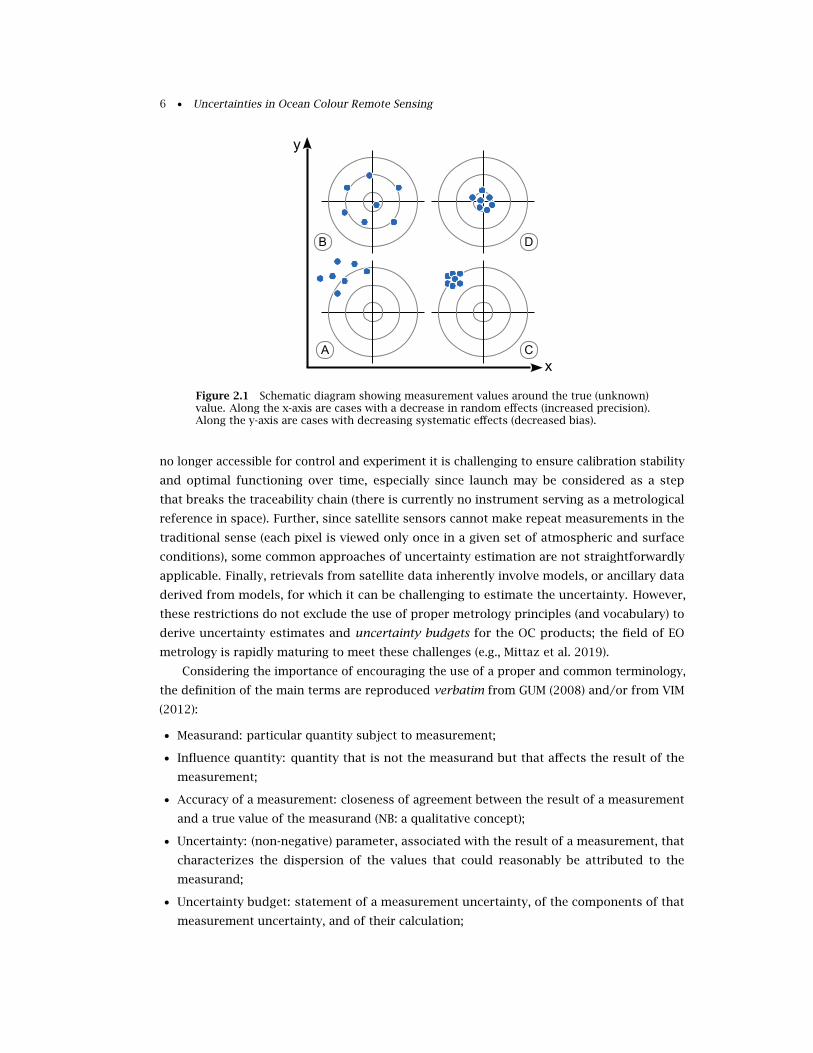
Some of these definitions can be graphically illustrated in Figure 2.1, where measurement
values are displayed around the true value of a measurand. In the case A, repeated measure-
ments show a significant level of dispersion with an average that would also be far from the
true value. Assuming that the measurement values displayed are representative of a much
larger population, both random and systematic errors are high. It is recalled that these error
terms are not known; however, if a proper method to determine uncertainty is set up, the
result would be a high value of uncertainty. The case B is different: even though the dispersion
is still high, the average of the measurement values is actually close to the true value, with a
much smaller systematic error. Along the same line, it means that measurement trueness is
better than for case A, again assuming that the displayed values are representative of a much
larger population. Uncertainty estimate still would be likely high but systematic effects do not
contribute much to it. The case C is opposite to B as far as the relative weight of random and
systematic effects is concerned. In that case the measurement system can be deemed as having
a good precision, a good repeatability if the conditions of measurements are maintained, or a
good reproducibility if some measurement conditions have changed (like a different location,
operator or measuring system). However systematic effects still contribute significantly to the
uncertainty of the measurements. Finally D is the ideal case, with a good precision and a small
bias.
The above metrological concepts have primarily been defined and applied in the context
of practical measurements in science and industry but their application to Earth Observation
(EO) presents a significant challenge for several reasons. Firstly, error-correlation between
pixel measurements is much more complex than the simple laboratory case. Errors in satellite
imagery are typically correlated with different functional forms based on their separation in
different spatial, temporal and spectral dimensions. An understanding of this structure is
important when data processing steps combine data, for example, from different spectral
channels or spatial pixels (e.g., regridding). Additionally, since the measurement instrument is
6 • Uncertainties in Ocean Colour Remote Sensing
Figure 2.1 Schematic diagram showing measurement values around the true (unknown)value. Along the x-axis are cases with a decrease in random effects (increased precision).Along the y-axis are cases with decreasing systematic effects (decreased bias).
no longer accessible for control and experiment it is challenging to ensure calibration stability
and optimal functioning over time, especially since launch may be considered as a step
that breaks the traceability chain (there is currently no instrument serving as a metrological
reference in space). Further, since satellite sensors cannot make repeat measurements in the
traditional sense (each pixel is viewed only once in a given set of atmospheric and surface
conditions), some common approaches of uncertainty estimation are not straightforwardly
applicable. Finally, retrievals from satellite data inherently involve models, or ancillary data
derived from models, for which it can be challenging to estimate the uncertainty. However,
these restrictions do not exclude the use of proper metrology principles (and vocabulary) to
derive uncertainty estimates and uncertainty budgets for the OC products; the field of EO
metrology is rapidly maturing to meet these challenges (e.g., Mittaz et al. 2019).
Considering the importance of encouraging the use of a proper and common terminology,
the definition of the main terms are reproduced verbatim from GUM (2008) and/or from VIM
(2012):
• Measurand: particular quantity subject to measurement;
• Influence quantity: quantity that is not the measurand but that affects the result of the
measurement;
• Accuracy of a measurement: closeness of agreement between the result of a measurement
and a true value of the measurand (NB: a qualitative concept);
• Uncertainty: (non-negative) parameter, associated with the result of a measurement, that
characterizes the dispersion of the values that could reasonably be attributed to the
measurand;
• Uncertainty budget: statement of a measurement uncertainty, of the components of that
measurement uncertainty, and of their calculation;
Terminology and Main Principles • 7
• Error: result of a measurement minus a true value of the measurand (which in practice
will never be known) or minus a reference quantity value (assumed to have a negligible
uncertainty);
• Random error: result of a measurement minus the mean that would result from an infinite
number of measurements of the same measurand carried out under repeatability conditions;
• Systematic error: mean that would result from an infinite number of measurements of
the same measurand carried out under repeatability conditions minus a true value of the
measurand;
• Traceability: property of a measurement result whereby the result can be related to a
reference through a documented unbroken chain of calibrations, each contributing to the
measurement uncertainty.
Besides these fundamental characteristics of the measurands and their uncertainties,
some other terms relevant to the report can be briefly discussed here. According to the
definition in VIM (2012), verification provides objective evidence that a given item fulfills
specific requirements, which becomes validation when the specified requirements are adequate
for an intended use. In remote sensing disciplines “validation” is generally intended as the
“process of assessing, by independent means, the quality of data products” (Justice et al.
2000, as formulated by the Committee on Earth Observation Satellites, CEOS). In that context,
speaking of “validation of uncertainties” is justified if the data products are the uncertainty
estimates. As the “independent means” have often been understood as reference data typically
derived from field observations, “validation” has usually been seen as a comparison between
satellite products and field data, a use that is also employed in this report but that has only
partial adherence to the metrological definition. The concept of validation has also been
extended to a more general quality assessment of OC products (Volpe et al. 2012). The term
“verification” has not been largely employed in OC remote sensing so that the metrological
definition could easily be adopted for the process of checking that stated uncertainties fulfill
the requirements for the considered data product.
Finally, the concept of metrological compatibility refers to the “property of a set of
measurement results, such that the absolute value of the difference of any pair of measured
quantity values from two different measurement results is smaller than some chosen multiple
of the standard measurement uncertainty of that difference” (VIM 2012), which basically means
that the two quantities being compared agree within their stated uncertainty. This term is fully
relevant when comparing two satellite data products, or satellite and field data.

8 • Uncertainties in Ocean Colour Remote Sensing
Chapter 3
Sources of Uncertainties
Frédéric Mélin, Emmanuel Boss, Barbara Bulgarelli, Roland Doerffer, Bryan A.
Franz, Martin Hieronymi, Chuanmin Hu, Ewa Kwiatkowska, Griet Neukermans,
Menghua Wang and P. Jeremy Werdell
Uncertainty terms can be divided into those of epistemic nature, originating from a lack of
knowledge about the processes to be represented, and those related to the inherent (like
stochastic) variability of any natural system (e.g., Walker et al. 2003; Der Kiureghan and
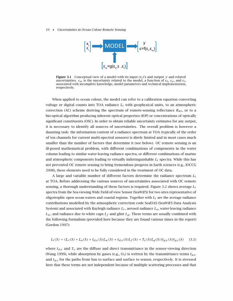
Ditlevsen 2009). Figure 3.1 represents a conceptual view of a model with its input/output
flow and their related uncertainties. The uncertainty ε associated with the output y results
from four main sources. First, input variables (xi)’s (influence quantities in an algorithm)
are characterized by their own uncertainties (εi)’s that are propagated through the model
that is itself a source of uncertainties. The epistemic uncertainty εk (also termed structural
uncertainty) results from phenomena that are insufficiently known or represented in the model,
with the corollary that it can be reduced if additional knowledge or complexity are brought in
the model. Part of this uncertainty may actually be accepted when a particular phenomenon is
ignored or simplified under the assumption that it is responsible for negligible uncertainties.
Even if the model structure is complete in its representation of all phenomena, some model
parameters may not be fully characterized, leading to a parameter uncertainty term εp . Finally,
complex models running on computers often include a discretization in time or space or
various numerical approximations (including those associated with machine precision) that
can contribute a technical (or numerical) uncertainty εt to the model results. To these four
categories, one of representation may be added: in the context of Earth observation, the
primary datum is associated with a satellite footprint while final products usually come as
gridded data for a specific time interval (e.g., daily, monthly), and this process of data editing
(including re-mapping or binning) has its own uncertainty. Eventually sources of uncertainty
can be distributed in the following categories:
v Input uncertainties
v Model structure / parameter uncertainties
v Numerical/technical uncertainties
v Editing uncertainties
9
10 • Uncertainties in Ocean Colour Remote Sensing
Figure 3.1 Conceptual view of a model with its input (xi)’s and output y and relateduncertainties. εm is the uncertainty related to the model, a function of εk, εp , and εt ,associated with incomplete knowledge, model parameters and technical implementation,respectively.
When applied to ocean colour, the model can refer to a calibration equation converting
voltage or digital counts into TOA radiance Lt with geophysical units, to an atmospheric
correction (AC) scheme deriving the spectrum of remote-sensing reflectance RRS , or to a
bio-optical algorithm producing inherent optical properties (IOP) or concentrations of optically
significant constituents (OSC). In order to obtain reliable uncertainty estimates for any output,
it is necessary to identify all sources of uncertainties. The overall problem is however a
daunting task: the information content of a radiance spectrum at TOA (typically of the order
of ten channels for current multi-spectral sensors) is direly limited and in most cases much
smaller than the number of factors that determine it (see below). OC remote sensing is an
ill-posed mathematical problem, with different combinations of components in the water
column leading to similar water-leaving radiance spectra, or different combinations of marine
and atmospheric components leading to virtually indistinguishable Lt spectra. While this has
not prevented OC remote sensing to bring tremendous progress in Earth sciences (e.g., IOCCG
2008), these elements need to be fully considered in the treatment of OC data.
A large and variable number of different factors determine the radiance spectrum Ltat TOA. Before addressing the various sources of uncertainties associated with OC remote
sensing, a thorough understanding of these factors is required. Figure 3.2 shows average Ltspectra from the Sea-viewing Wide Field-of-view Sensor (SeaWiFS) for two sites representative of
oligotrophic open ocean waters and coastal regions. Together with Lt are the average radiance
contributions modelled by the atmospheric correction code SeaDAS (SeaWiFS Data Analysis
System) and associated with Rayleigh radiance Lr , aerosol radiance La, water-leaving radiance
Lw , and radiance due to white caps Lf and glint Lg . These terms are usually combined with
the following formalism (provided here because they are found various times in the report)
(Gordon 1997):
Lt(λ) = (Lr (λ)+ La(λ)+ td,v(λ)Lw(λ)+ td,v(λ)Lf (λ)+ Tv(λ)Lg(λ))tg,v(λ)tg,s(λ) (3.1)
where td,v and Tv are the diffuse and direct transmittance in the sensor-viewing direction
(Wang 1999), while absorption by gases (e.g., O3) is written by the transmittance terms tg,vand tg,s for the paths from Sun to surface and surface to sensor, respectively. It is stressed
here that these terms are not independent because of multiple scattering processes and that
Sources of Uncertainties • 11
possible impacts from clouds or adjacent land are ignored.
gases (O2,N2,O3, NO2,…)aerosols
clouds, cloud reflec�on & shadowscontrails,
…
AAOTMOBYLtLr
La
Lg
Lw
Lf
LtLrLa
Lg
LwLf
water op�cal proper�es(pure water,
phytoplankton,dissolved organic ma�er,
non-algal par�cles…)bo�om reflec�on,
…
sun glintfoam, bubbles
floa�ng materialadjacency (land, ice)
…
Figure 3.2 Average of radiance spectra from SeaWiFS over the Marine Optical Buoy(MOBY, left-hand panel) oligotrophic site near Hawaii and the coastal Acqua Alta Ocea-nographic Tower (AAOT, right-hand panel). Averages are obtained for conditions wherethe SeaDAS atmospheric correction produced a valid water-leaving radiance Lw (thegreen dotted line on the left-hand plot indicate Lw values going to 0, which is not wellrepresented on a logarithmic scale). Lt is the TOA radiance, Lr , La, Lg , Lf are radianceterms due to air molecules (Rayleigh), aerosol, glint, and white caps (foam), respectively.Example actors contributing to Lt are grouped into those associated with atmospheric(blue), surface (grey) and sub-surface (green) processes.
Importantly, the averages shown in Figure 3.2 are computed including only cases where
the AC has produced valid Lw spectra, which means that various atmospheric situations (such
as cloudy skies) are filtered out. Figure 3.2 also names a non-exhaustive list of potential
contributors to Lt grouped into three main categories, as associated with atmospheric actors,
surface phenomena and sub-surface actors. From the comparison of the two sets of radiance
spectra, common points and differences can be noticed. In both cases, the TOA signal is
mostly the result of scattering and absorption by atmospheric constituents (molecules and
aerosols) while Lw accounts for a small fraction of the radiance budget (Gordon 1987), with
differences in amplitude and spectral shape between the two sites (the oligotrophic site showing
characteristically high values in the blue and low values in the red, while the coastal site has
a spectral maximum at 555 nm). Contributions by white caps (or surface foam) and glint
12 • Uncertainties in Ocean Colour Remote Sensing
(specular reflection by the sea surface) are orders of magnitude lower but vary according to
the local wind regime and observation and illumination geometry, respectively. As mentioned
above, the spectra shown in Figure 3.2 are average situations, so that more extreme conditions
can occur; moreover, only conditions leading to a successful atmospheric correction by one
particular code are included, which means that, for instance, strong winds (speed larger than
12 m s−1) or high glint are not considered while they can actually be responsible for significant
radiance contributions.
Level-2 (a)
Level-1
Level-2 (b)
Level-3
TOA radiance Lt
- noise- uncertainties on sensor elements - straylight- polarization- aging
water-leaving radiance Lw
remote sensing reflectance RRS
mapped products
- aerosols - clouds- glint- adjacency effects- waves
- specific optical properties- assumed optical parameters- multiple scattering- inelastic scattering processes- bidirectional effects- vertical structure- bubbles- bottom reflectance
- spatial mismatch and heterogeneity- temporal inhomogeneity
inherent optical properties (a, bb)
concentrations of optically significant constituents(Chl-a, SPM, DOC, POC, ...)
signal at sensor
atmosphericcorrection
bio
-op
tica
lal
go
rith
m
calibration
gridding/binning
Figure 3.3 Schematic representation of ocean colour processing from level-1 to level-3. Itemized blacks elements are non-exhaustive lists of potential contributors to theuncertainty of the derived product.
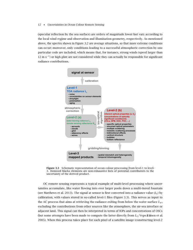
OC remote sensing represents a typical example of multi-level processing where uncer-
tainties accumulate, like water flowing into ever larger pools down a multi-tiered fountain
(see Matthews et al. 2013). The signal at sensor is first converted into a radiance value (Lt) by
calibration, with values stored in so-called level-1 files (Figure 3.3). This serves as input to
the AC process that aims at retrieving the radiance exiting from below the water surface Lw ,
excluding the contributions from other sources like the atmosphere, the air-sea interface or
adjacent land. This signal can then be interpreted in terms of IOPs and concentrations of OSCs
(but some attempts have been made to compute the latter directly from Lt ; Vepsäläinen et al.
2005). When this process takes place for each pixel of a satellite image (constructing level-2
Sources of Uncertainties • 13
files), a further (editing) step required for most user applications is the spatial gridding of the
pixel-wise information onto a geographic grid. The results obtained for each satellite overpass
are then combined for a day or longer periods into time composites (level-3 products). Figure
3.3 shows some of the factors contributing to the uncertainties along these steps. Logically,
as one goes through the successive levels of processing, with more factors playing a role, it
is expected that uncertainties will in general increase or at least that their determination will
become more arduous (Mittaz et al. 2019). For instance it is well accepted that uncertainties
on Lw are typically an order of magnitude higher than for Lt considering the small weight of
Lw in the radiance budget (Figure 3.2). This view of how uncertainties impact the overall OC
processing is simplified but nevertheless useful to start exploring a comprehensive uncertainty
budget.
Having set the stage for OC processing, our present knowledge about various sources of
uncertainties is now presented and discussed. Section 3.1 addresses sources of uncertainties
associated with input data (influence quantities in algorithms), while Section 3.2 focuses on
epistemic uncertainties, related to the incomplete knowledge or understanding of complex na-
tural phenomena, or their simplified representations in models (model structure and parameter
uncertainties). Section 3.3 discusses the issues of representation and editing.
3.1 Uncertainties in Input Data
3.1.1 Top-of-Atmosphere Data
The starting point for all OC products are the TOA spectra. Considering that the signal of
interest for ocean colour (water-leaving radiance) is a fairly small part of the TOA signal (Figure
3.2), it has been recognized early on that ocean colour is particularly demanding in terms
of calibration (Gordon 1987) and related requirements have been stated on calibration and
signal-to-noise ratios (IOCCG 1998). Ocean colour requires a well calibrated sensor with a
high radiometric sensitivity (i.e., a high signal-to-noise ratio, SNR) and a long term stability
(IOCCG 2012). Besides a good knowledge of the platform position and possible orbit drift,
all the sensor radiometric and spectral properties must be well characterized pre-launch and
on-orbit to perform the sensor radiometric calibration: sensor spectral response function, dark
current, radiometric angular dependency (response-versus-scan angle), detector-to-detector
differences, linearity (or variations around it), sensitivity for polarized light and straylight,
out-of-band response (Gordon 1995), temperature dependence, etc. For instance, sensitivity to
the polarization associated with the radiance field exiting the atmosphere can be significant for
some sensors, e.g., ∼3% in the blue for MODIS (Moderate Resolution Imaging Spectroradiometer)
or VIIRS (Visible Infrared Imager Radiometer Suite) (Meister et al. 2005; Sun et al. 2016). As
far as possible, these properties have to be monitored during the life time of the sensor.
Any deviations must be compensated by correction procedures, because a small bias in the
order of a few percent in TOA radiances may have a large impact on the derived water-leaving
radiances. The residual uncertainty has to be quantified and included in the overall uncertainty
budget. For this, all the relevant elements need to be properly represented and modelled in
14 • Uncertainties in Ocean Colour Remote Sensing
the calibration equation. Once on orbit, calibration relies on on-board devices making use
of internal light sources or external targets (Sun, Moon), each set-up having advantages and
limitations (IOCCG 2013). The experience from the CZCS (Coastal Zone Color Scanner) mission
demonstrated the deleterious effects that sensor degradation could have on the OC products
(Evans and Gordon 1994). With more recent missions, the use of on-board solar diffusers and
lunar measurements have been instrumental in guaranteeing stability to the OC record (Barnes
et al. 2001; Sun and Wang 2015; Xiong et al. 2016). For instance, Eplee et al. (2012) evaluate
the long-term stability of the SeaWiFS TOA radiance within 0.13% (0.30% if incorporating the
vicarious calibration process).
Currently the lowest uncertainties associated with TOA radiance are broadly of the order of
3–5%, to be compared with the <5% mission objective for SeaWiFS TOA radiance (Hooker et al.
1992). For instance, Johnson et al. (1999) presented an uncertainty analysis for the prelaunch
calibration of SeaWiFS, leading to a 3% value, and compared two calibration experiments that
agreed within 4%. The differences obtained on-orbit with respect to a radiative model of the
Moon are 2–3% in Eplee et al. (2012). Barnes et al. (2001) proposed to decompose the total
uncertainty for SeaWiFS on-orbit observations into 3% for pre-launch calibration (Johnson
et al. 1999), 3% for the transfer to orbit (Barnes et al. 2000) and 1% for instrument changes
derived from lunar measurements, leading (as root sum square) to 4.4% for SeaWiFS TOA
radiance. From an uncertainty budget conducted for MODIS, Esposito et al. (2004) stated
uncertainties of 5% in radiance and 2% in reflectance factor. IOCCG (2013) evaluates at 3% the
uncertainty associated with a radiance-based calibration of MERIS (Medium Resolution Imaging
Spectrometer) through a solar diffuser, taking into account the uncertainty of solar irradiance
(∼2% as a 2-σ , or k=2, uncertainty for 1-nm resolution spectral values in Thuillier et al. 2003),
a term that can be factored out when working with reflectance spectra. Differences between
1% and 8% were observed between on-orbit lunar observations conducted by SeaWiFS, MODIS
Aqua and Terra (1–3% between the two MODIS, Eplee et al. 2011).
Ultimately, uncertainties of 2% for TOA radiance has been proposed as a realistic target,
although still lower uncertainties would be certainly welcome (IOCCG 2012). To give further
context on these values, it can be noticed that current irradiance standards used for calibration
have an uncertainty close to 1% (Yoon et al. 2002) while uncertainties associated with a
laboratory characterization of a bidirectional reflectance factor of a solar diffuser can be ∼1.5%
(Esposito et al. 2004). However, new developments in instruments or lunar measurements
could help further progress (Cramer et al. 2013; Levick et al. 2014).
Considering the uncertainty values reported above for TOA radiance, together with the
rule of thumb that an uncertainty at TOA is multiplied by 10 when the water-leaving radiance
is obtained (considering the weight of Lw in a typical radiance budget, Figure 3.2), it appeared
that an additional step was needed to better constrain the absolute radiometric calibration
of OC sensors and reach mission objectives like a 5% uncertainty in Lw for open ocean
waters (Hooker et al. 1992). Calibration practices using Earth targets and/or surface and
atmospheric measurements coupled with radiative transfer calculations (Gordon and Zhang
1996; Martiny et al. 2005; IOCCG 2013) provide accuracy estimates (>1%) deemed insufficient
for OC applications. So, a practice of OC vicarious calibration (VC) has been introduced that
Sources of Uncertainties • 15
adjusts calibration coefficients to force agreement with reference field measurements of Lw(Gordon 1987; Zibordi et al. 2015). The standard way of operating VC for OC sensors is to
propagate highly accurate in situ Lw measurements in the visible to TOA using the same
atmospheric radiative model used in the atmospheric correction (e.g., Franz et al. 2007). VC
gain factors are then derived as the ratio between simulated and measured Lt values. For
standard AC codes, NIR bands need to be well calibrated prior to running this procedure for
the visible bands (see Franz et al. 2007 for an example). The overall process is referred to
as System Vicarious Calibration (SVC) since it applies to the system ‘sensor + atmospheric
correction’. The precision associated with SVC (computed as the standard deviation of the
mean, or standard deviation of the gain factors divided by the square root of the number of
samples) can be below 0.1% if a sufficient number of calibration points have been gathered
(Franz et al. 2007).
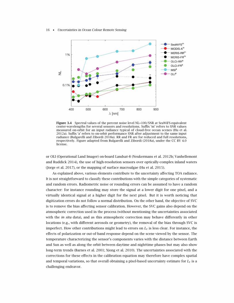
One part of the uncertainty characterizing Lt can be classified as noise, originating from
the electronic noise that affects acquisition system and from rounding errors. TOA noise,
contributing to random error for Lt , has a direct impact on the noise affecting the retrieved
quantity and the capacity to distinguish specific patterns (Hu et al. 2001a, 2013). It is often
quantified by the signal-to-noise ratio (SNR, a TOA typical Lt value divided by the noise signal)
that is listed among the pre-launch specifications (Hooker et al. 1992; Rast et al. 1999; Xiong
et al. 2010; Donlon et al. 2012). Post-launch SNR levels have been checked using on-board
devices (like solar diffusers, Eplee et al. 2012) or homogeneity tests on clear-water regions (Hu
et al. 2012b). SNR values for SeaWiFS are of the order of 420–790 in the visible domain and
around 200 in the near-infrared, while they are higher for later sensors such as MODIS or OLCI
(Ocean and Land Colour Instrument, on-board Sentinel-3) for its reduced-resolution bands (Hu
et al. 2012a; Donlon et al. 2012). Taking the inverse, this means a noise level (NL) for SeaWiFS
Lt of 0.15-0.2% and 0.5% in the visible and NIR (Near Infra-Red), respectively (Hu et al. 2012a;
Eplee et al. 2012). Figure 3.4 illustrates NL for a representative set of satellite missions.
Considering the overall uncertainty on Lt , the contribution from the noise is actually fairly
small. However, depending on the quantity of interest and the associated algorithm, it is
sufficient to generate significant uncertainties in derived products, particularly through the
impact of higher noise levels usually found in the NIR bands used in atmospheric correction
schemes (e.g., Moses et al. 2012; Jorge et al. 2017). For instance, it can easily lead to 10%
or more uncertainty in chlorophyll-a concentration (Chl-a) values derived by a blue-green
band-ratio algorithm in oligotrophic waters (Hu et al. 2013). For general applications, SNR of
1000, 600 and 200 are recommended in the visible, NIR and SWIR (Short-Wave Infra-Red) bands,
respectively (IOCCG 2012; Wang and Gordon 2018); these levels can actually be somewhat
relaxed for standard applications like computing Chl-a in open ocean waters (Gordon 1990;
Hu et al. 2013; Qi et al. 2017b). Additional studies have been carried out to address the
relationship between SNR and uncertainty associated with the derived product of interest
when using sensors or bands not originally developed for ocean colour and/or for specific
applications, including the use of SWIR bands for atmospheric correction (Wang and Shi 2012;
Wang and Gordon 2018), the determination of suspended matter concentration using sensors
of low radiometric sensitivity such as SEVIRI (Spinning Enhanced Visible and Infrared Imager)
16 • Uncertainties in Ocean Colour Remote Sensing
Figure 3.4 Spectral values of the percent noise level NL=100/SNR at SeaWiFS-equivalentcenter-wavelengths for several sensors and resolutions. Suffix ‘m’ refers to SNR valuesmeasured on-orbit for an input radiance typical of cloud-free ocean scenes (Hu et al.2012a). Suffix ‘a’ refers to on-orbit performance SNR after adjustment to the same inputradiance (Bulgarelli and Zibordi 2018a). RR and FR are for reduced and full resolutions,respectively. Figure adapted from Bulgarelli and Zibordi (2018a), under the CC BY 4.0license.
or OLI (Operational Land Imager) on-board Landsat-8 (Neukermans et al. 2012b; Vanhellemont
and Ruddick 2014), the use of high-resolution sensors over optically-complex inland waters
(Jorge et al. 2017), or the mapping of surface macroalgae (Hu et al. 2015).
As explained above, various elements contribute to the uncertainty affecting TOA radiance.
It is not straightforward to classify these contributions with the simple categories of systematic
and random errors. Radiometric noise or rounding errors can be assumed to have a random
character: for instance rounding may store the signal at a lower digit for one pixel, and a
virtually identical signal at a higher digit for the next pixel. But it is worth noticing that
digitization errors do not follow a normal distribution. On the other hand, the objective of SVC
is to remove the bias affecting sensor calibration. However, the SVC gains also depend on the
atmospheric correction used in the process (without mentioning the uncertainties associated
with the in situ data), and as this atmospheric correction may behave differently in other
locations (e.g., with different aerosols or geometry), the removal of the bias through SVC is
imperfect. How other contributions might lead to errors on Lt is less clear. For instance, the
effects of polarization or out-of-band response depend on the scene viewed by the sensor. The
temperature characterizing the sensor’s components varies with the distance between Earth
and Sun as well as along the orbit between daytime and nighttime phases but may also show
long-term trends (Barnes et al. 2001; Xiong et al. 2010). The uncertainties associated with the
corrections for these effects in the calibration equation may therefore have complex spatial
and temporal variations, so that overall obtaining a pixel-based uncertainty estimate for Lt is a
challenging endeavor.
Sources of Uncertainties • 17
A last word is due for the process of sensor inter-calibration that has been regularly
employed to tune the calibration of one space sensor with data from another mission deemed
better calibrated (Wang and Franz 2000; Hu et al. 2001b; Pan et al. 2004; Kwiatkowska et al.
2008; Eplee et al. 2011; Meister et al. 2012). In such a case, determining an uncertainty value
for the target sensor is still more complex since the uncertainty budgets for both sensors are
involved as well as the uncertainty associated with the transfer process.
3.1.2 Ancillary Data
For the interpretation of OC observations ancillary data are necessary, in particular for the
correction of the influence of the atmosphere. Depending on the mission, these data, such as
ozone, pressure, wind speed, water vapour, NO2, come from the re-analysis of weather forecast
data, from other satellite missions, or from a climatology of these variables. In any case all of
them have their own uncertainties and, thus, have an impact on the accuracy of the OC data.
The process of atmospheric correction has been shown to be sensitive, in a varying amount, to
the uncertainties associated with ancillary data (Ramachandran and Wang 2011).
Concentration of sea ice has been mainly used as ancillary information to help in excluding
data from the atmospheric correction process and set up an appropriate flag. Sea ice distribu-
tion could also be used for an improved consideration of the adjacency effects generated by
the bright surface usually associated with sea ice (Bélanger et al. 2007).
Atmospheric pressure (Pa) is an important element for atmospheric correction since it has
a direct impact on Rayleigh scattering and atmospheric transmittance. It is usually provided
by global distributions from Numerical Weather Predictions (NWP) centers such as the US
National Centers for Environmental Predictions (NCEP) or the European Centre for Medium-
Range Weather Forecasts (ECMWF) with a typical 6-hour time resolution. From comparisons
between ECMWF and NCEP analyses and with island data, Ponte and Dorandeu (2003) suggest
uncertainties of the order 1-2 hPa (with values higher in the Southern Ocean). With a good ap-
proximation, Rayleigh radiance can be considered proportional to (1-exp(−τr/ cosθ)) (Gordon
et al. 1988a), where θ is the viewing zenith angle and τr the Rayleigh optical thickness, itself
proportional to Pa (neglecting variations due to acceleration of gravity or molecular weight of
air, Bodhaine et al. 1999). So, an error of 1 hPa or 4 hPa would lead to an error in Rayleigh
radiance Lr in the visible of 0.08-0.09% and 0.34%, respectively, at a wavelength of 440 nm and
for θ=30◦. Even though these numbers are small, it must be recalled that Lr represents a large
share of the radiance budget and is approximately an order of magnitude higher than Lw in
the blue spectral domain (Figure 3.2). Atmospheric pressure may also have an impact on Ltthrough radiatively-significant gases when their concentrations vary with Pa, such as oxygen at
the 765-nm SeaWiFS band (Ding and Gordon 1995).
Wind is pervasive in OC remote sensing. By its impact on the roughness of the sea surface
(expressed by the mean-square slope of the wave field) it modifies the radiance reflectance and
transmittance distribution of the air-sea interface and has therefore an impact on the diffusivity
of the under-water light field near the surface and the water-leaving radiance (Hieronymi 2016).
This modification of the boundary condition needs to be taken into account in the atmospheric
18 • Uncertainties in Ocean Colour Remote Sensing
correction, for instance in the calculation of the Rayleigh radiance (Gordon and Wang 1992;
Wang 2002), while below the surface, the different orientations of the wave surface modulate
the light rays going through it (e.g., by focusing/defocusing effects, Zaneveld et al. 2001;
D’Alimonte et al. 2010). However, the relationship between IOPs and Lw is affected by wind
only at high speeds (Gordon 2005). Through its impact on wave geometry, wind also has an
effect on glint patterns (Cox and Munk 1954; Kisselev and Bulgarelli 2004). It is worth stressing
here that wave characteristics also depend on swell and not only on local wind (Hanley et al.
2010).
Other than geometry the wind regime ultimately impacts the upper ocean by generating
bubbles accumulating at the surface as white caps, the high-latitude regions being characterized
by the highest white cap fractions (Salisbury et al. 2014). Breaking waves also ingest bubbles
below the surface that can have a noticeable impact on the in-water light field (e.g., Terrill et al.
2001; Stramski and Tegoswki 2001; Piskozub et al. 2009). Because of these effects that are
not necessarily easy to model (see below), a threshold on wind speed is enforced for some
standard atmospheric corrections: above that value, the processing is not performed (for
instance, in the case of SeaDAS/l2gen, this limit is set at 12 m s−1, which is fairly strict as some
trade winds may exceed that value). As an implication, a bias affecting the wind field used as
ancillary data has a direct impact on the coverage of the satellite products. As atmospheric
pressure, wind fields for OC processing are usually provided by NWP outputs. Comparisons
between NWP and satellite wind products documented root-mean-square (RMS) differences in
the interval 1–3 m s−1 depending on the region while comparison between wind scatterometry
products and buoy data typically showed RMS differences of the order of 1 m s−1 (Chelton
and Freilich 2005; Chaudhuri et al. 2013). Multi-year biases may reach 0.5 m s−1 for some
NWP products (Chelton and Freilich 2005; Wallcraft et al. 2009). As for wind speed, the Global
Climate Observing System (GCOS) gives an uncertainty target for satellite products of 0.5 m
s−1 (GCOS 2011). Another factor possibly contributing to the uncertainty in the wind products
used for OC processing is the mis-match in spatial resolution: NWP fields are typically provided
with a resolution of the order of a quarter to one degree, which might be insufficient to resolve
specific features associated with coast lines or island wakes (Xie et al. 2001; Risien and Chelton
2008) and might lead to downscaling errors.
As well provided by NWP products, relative humidity (RH) is used by some atmospheric
correction schemes to help in the choice of aerosol models (Ahmad et al. 2010). Uncertainties
associated with RH fields vary regionally but systematic differences of the order of 10% may be
found (John and Soden 2007; Vergados et al. 2015), which might locally affect the choice of
aerosols.
In the visible channels, ozone absorbs light between 500 and 700 nm with maximum
absorption around 600 nm. The two-way absorption (Sun to Earth and Earth to satellite) must
be corrected accurately as it affects the observed Lt (Equation 3.1). In practice, daily ozone
measurements from several satellites (e.g., TOMS, TOVS) or NWP products (ECMWF) are used to
correct the O3 absorption efficiently and compute Lt for a hypothetical ozone-free atmosphere.
Within a range of about 240 – 400 Dobson units (DU), these products have uncertainties
typically within 5% (Bhartia 2002; Lerot et al. 2014) with a GCOS requirement of 5 DU or 2%
Sources of Uncertainties • 19
(GCOS 2011). When such data are not available, daily climatology are used instead, which
contain higher uncertainties due to interannual changes on the same day of the year, the
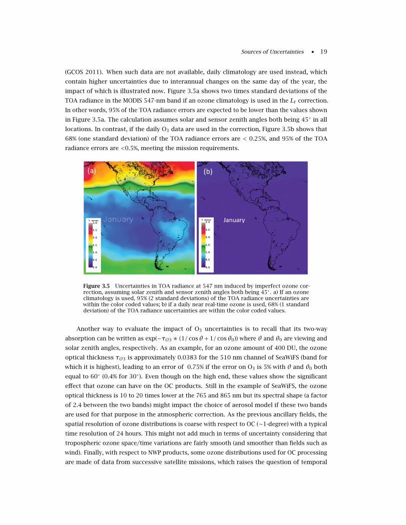
impact of which is illustrated now. Figure 3.5a shows two times standard deviations of the
TOA radiance in the MODIS 547-nm band if an ozone climatology is used in the Lt correction.
In other words, 95% of the TOA radiance errors are expected to be lower than the values shown
in Figure 3.5a. The calculation assumes solar and sensor zenith angles both being 45◦ in all
locations. In contrast, if the daily O3 data are used in the correction, Figure 3.5b shows that
68% (one standard deviation) of the TOA radiance errors are < 0.25%, and 95% of the TOA
radiance errors are <0.5%, meeting the mission requirements.
Figure 3.5 Uncertainties in TOA radiance at 547 nm induced by imperfect ozone cor-rection, assuming solar zenith and sensor zenith angles both being 45◦. a) If an ozoneclimatology is used, 95% (2 standard deviations) of the TOA radiance uncertainties arewithin the color coded values; b) if a daily near real-time ozone is used, 68% (1 standarddeviation) of the TOA radiance uncertainties are within the color coded values.
Another way to evaluate the impact of O3 uncertainties is to recall that its two-way
absorption can be written as exp(−τO3 ∗ (1/ cosθ+ 1/ cosθ0)) where θ and θ0 are viewing and
solar zenith angles, respectively. As an example, for an ozone amount of 400 DU, the ozone
optical thickness τO3 is approximately 0.0383 for the 510 nm channel of SeaWiFS (band for
which it is highest), leading to an error of 0.75% if the error on O3 is 5% with θ and θ0 both
equal to 60◦ (0.4% for 30◦). Even though on the high end, these values show the significant
effect that ozone can have on the OC products. Still in the example of SeaWiFS, the ozone
optical thickness is 10 to 20 times lower at the 765 and 865 nm but its spectral shape (a factor
of 2.4 between the two bands) might impact the choice of aerosol model if these two bands
are used for that purpose in the atmospheric correction. As the previous ancillary fields, the
spatial resolution of ozone distributions is coarse with respect to OC (∼1-degree) with a typical
time resolution of 24 hours. This might not add much in terms of uncertainty considering that
tropospheric ozone space/time variations are fairly smooth (and smoother than fields such as
wind). Finally, with respect to NWP products, some ozone distributions used for OC processing
are made of data from successive satellite missions, which raises the question of temporal
20 • Uncertainties in Ocean Colour Remote Sensing
consistency.
Nitrogen dioxide (NO2) also has an impact on absorption of light with a fairly broad
absorption spectrum with a peak at approximately 412 nm. Some investigations based on
radiative transfer simulations have shown that, in conditions of large NO2 load, neglecting
the impact from NO2 is equivalent to an error at the top-of-atmosphere of ∼1% at 412 nm for
sensors like SeaWiFS or MODIS (Ahmad et al. 2007). Considering that errors at TOA translates
in errors on Lw higher by an order of magnitude, a proper description of the NO2 distribution
and its effect in the process of atmospheric correction is recommended to reduce uncertainties
on Lw . This is further supported by a recent study by Tziortziou et al. (2018) who highlight the
large variability that NO2 can display in coastal regions and the impact on the retrieved Lw of
ten’s of % if this variability is not taken in to account. Uncertainties affecting NO2 fields can be
of a few ten’s of percent (Boersma et al. 2004), but they are only relevant close to NO2 sources
on continents, except for some cases of long range transport or shipping emissions (Richter
et al. 2004). One issue associated with NO2 is the fact that satellite input sources do not cover
the entire OC record, so that climatological fields have been preferred to ensure consistency.
Temperature and salinity ancillary values can also be used in ocean colour processing
(Werdell et al. 2013a) since they affect the inherent optical properties of pure seawater (Sullivan
et al. 2006; Zhang et al. 2009). The backscattering by pure seawater bbw can show variations
of 25% along salinity (primarily) and temperature gradients. Climatological fields have been
used in OC processing, which tends to increase uncertainties, particularly in coastal regions
such as estuaries. On the other hand, those are regions where bbw is much lower than the
backscattering signal associated with particles. Absorption variations due to temperature or
salinity are fairly small and insignificant below 550 nm (Sullivan et al. 2006).
Considering the elements provided in this section, the ocean colour community should
devote more attention for collecting a comprehensive picture of the uncertainties affecting
ancillary data so that they can appropriately be propagated in OC algorithms. In that regard,
the emergence of NWP simulation ensembles might be extremely fruitful (Laloyaux et al. 2018).
3.2 Uncertainties Associated with Models and Algorithms
This Section addresses the sources of structural (epistemic) uncertainties associated with
model structure, model parameters, or insufficient knowledge or description of phenomena.
3.2.1 Atmosphere
The atmosphere is one of the major sources of uncertainties. Since over water, a large part
(often more than 90%) of the measured upward-directed radiance in the visible spectral range at
TOA is light scattered by the atmosphere (by molecules and aerosols in the standard OC cases),
any error in the determination of the atmospheric path radiance and transmittance potentially
leads to large errors in the determination of the water-leaving radiance. Thus, the so-called
atmospheric correction (AC) is key to the success of OC remote sensing while the sources of
uncertainties associated with this process remain complex and multi-faceted (Gordon 1997). A
Sources of Uncertainties • 21
pure “Rayleigh” atmosphere is not considered as a relevant source of uncertainties as long as
multiple scattering, polarization and sensor spectral response are taken into account (Gordon
et al. 1988a; Wang 2016), while current parameterizations can easily represent the effect of
variations in atmospheric pressure with uncertainties below 0.1% (often <0.05%) (Wang 2005).
Including the effects of Earth sphericity is also recommended, particularly for high solar zenith
angles (Ding and Gordon 1994; He et al. 2018).
Among the major atmospheric components, aerosols are the most variable in quantity
and properties. To perform the process of atmospheric correction, it is sufficient to represent
an accurate estimate of the aerosol radiance (or reflectance) in the AC process (explicitly or
not), while deriving other quantities such as aerosol optical thickness or other properties
that might be of interest for atmospheric science is secondary. Even though the practical
impact of including increased refinements about aerosol properties in AC algorithms can
be debatable (e.g., Stamnes et al. 2002), it is nonetheless expected that enhanced knowledge
on aerosol microphysical and optical properties can be translated in improvements in ACs.
Optical measurements of aerosol properties have considerably increased with the advent,
among other programs, of the Aerosol Robotic Network (AERONET). This provides data both
on land and across the oceans with its maritime component (Holben et al. 2001; Smirnov
et al. 2011), leading to a better definition of aerosols, including their marine components
particularly important for OC (Smirnov et al. 2003), and to revised aerosol models (Ahmad
et al. 2010). When explicitly represented in AC codes, these models typically rely on bi-
modal descriptions of the aerosol size distribution (with modes representing fine and coarse
particles) possibly modulated by relative humidity (e.g., Ahmad et al. 2010), from which
optical properties are derived (with appropriate assumptions such as Mie theory). However,
aerosols show a large diversity of shapes and constituents (e.g., Ebert et al. 2002) and faithfully
representing the related properties in AC algorithm is still a major challenge. Dust aerosols
are markedly complex in that respect: assumptions of sphericity often applied for aerosol
models are not always valid and can lead to significant uncertainties on optical properties
(Mishchenko et al. 1997; Kalashnikova and Sokolik 2002). The issue of absorption by aerosols
is specifically challenging: in a single scattering approximation, the radiance due to aerosols is
proportional to the product of single scattering albedo ωa and optical thickness τa, making
the determination of the aerosol component particularly difficult. AC schemes often make
assumptions about the aerosol vertical distribution, including relegating them to a boundary
layer below molecules, a two-layer system that achieves physical uncoupling between the
two components. Such assumptions may imply uncertainties in the AC process, a point that
becomes more relevant for absorbing aerosols (Ding and Gordon 1995; Antoine and Morel
1998; Duforêt et al. 2007). For these reasons the presence of absorbing aerosols is often
among the main reasons mentioned for poor results of the AC (e.g., Schollaert et al. 2003).
Aerosol polarization effects can also be significant (Wang 2006). With low observation and
solar zenith angles and pure maritime atmospheres (small τa), modeling the path radiance
is obviously easier and even single scattering approximations have been shown to provide
acceptable results. But in general, uncertainties related to aerosols tend to increase as soon as
aerosol loads, aerosol absorption and air masses increase.
22 • Uncertainties in Ocean Colour Remote Sensing
The importance of the correction of the path radiance increases with decreasing reflectance
of the water body. In the clear open ocean the reflectance in the red spectral range is low, due
to high absorption by water. The scattering by aerosols and in particular by air molecules is
also decreasing with increasing wavelength. In contrast, waters with high concentrations of
humic substances and phytoplankton have a low reflectance in the blue part of the spectrum.
Since in this spectral range scattering by molecules in the air and also by many aerosol types is
increasing, the ratio of water leaving radiance to the path radiance becomes extremely low and
thus the uncertainty of products such as chlorophyll or absorption by chromophoric dissolved
organic matter (CDOM) may dramatically increase.
The presence of land or clouds in the vicinity of water pixels can affect the radiance
collected by a sensor looking at these water pixels through the so-called adjacency effect (AE).
AEs always occur in the presence of a scattering atmosphere over a non-uniform reflecting
surface, which causes the radiance from high-reflectivity areas to spill over neighboring low-
reflectivity regions, thus modifying their apparent brightness (Otterman and Fraser 1979). If
not properly accounted for, AE leads to increased uncertainties on derived products. AEs are
discussed in more details below. For certain geometries, the effect of clouds can also manifest
itself as shadowing that causes low sensor-measured TOA radiance, leading to biased low
satellite-derived water-leaving radiance spectra.
Another issue is related to the absorption by atmospheric gases, in particular by oxygen,
ozone and water vapour, which are the dominating gases with absorption bands in the visible
to NIR spectral range. For most OC sensors the spectral bands have been placed in regions
outside the strong absorption bands of oxygen and water vapour (which might change with
the advent of sensors with many more bands). However, in some spectral bands there is
still some influence of these gases, e.g. in the range > 680 nm. Most atmospheric correction
algorithms include procedures to correct this influence (e.g., Ding and Gordon 1995), but
their imperfections in modelling the gas absorption contribute to the uncertainty budget.
The absorption by ozone with its broad absorption band in the visible range, which covers
important OC bands, has to be taken into account in any case (see previous Section 3.1.2).
3.2.2 Effects of Clouds, Ice and Land
The effect that bright targets (clouds, land, ice) can have on the retrieval associated with
adjacent pixels has been introduced above and is now discussed in more detail.
A pixel is commonly identified as cloud or ice if its Rayleigh and Sun glint corrected
reflectance in the NIR (∼860 nm) exceeds a certain limit. Although there are other approaches
to define clouds, this thresholding method has been used by NASA for global processing with
a threshold value of 0.027 (2.7% reflectance). The AE associated with clouds that impacts
TOA radiance over the ocean is analysed in this context. The AEs are flagged as straylight
for MODIS data processing, which is technically defined using a 7x5-pixel (along-scan x along-
track) dilation window around the cloud pixels. As a result, ∼50% of the cloud-free ocean
data are flagged as low quality. A recent study used clear-water scenes and statistics over
the North Atlantic and South Pacific to quantify the cloud AEs on TOA radiance and OC data
Sources of Uncertainties • 23
products for MODIS/Terra, MODIS/Aqua, and SeaWiFS measurements (Feng and Hu 2016a).
Results show that the AEs on TOA radiance share similar patterns among the three missions,
with significant AEs around clouds. AEs decrease monotonically with increasing distance
from clouds, but even at five 1-km pixels away the AEs still contribute a few percent to TOA
radiance for most visible bands. In addition, discernable memory effects are also observed on
cloud-adjacency pixels of both MODIS missions, representing >15% of the total AEs in TOA
radiance. The AEs on the retrieved remote sensing reflectance (RRS ) data products are different
among the three missions possibly due to differences in sensor design and uncertainties in
atmospheric correction, but at four 1-km pixels away from clouds the differences between
cloud-adjacent pixels are typically within 5% of pixels further away from clouds for most visible
bands. Large AEs (>50%) are observed in the normalized Fluorescence Line Height (nFLH) of
both MODIS/Terra and MODIS/Aqua. When the recently developed OCI (Ocean Color Index)
Chl-a algorithm (Hu et al. 2012b) is used, the current MODIS stray-light masking window (7x5)
used to flag the AE-contaminated pixels may be relaxed to 3x3 without sacrificing data quality,
leading to >40% of the previously masked low-quality data being recovered for clear waters
(Hu et al. 2019).
A further source of uncertainty are thin clouds and clouds that are smaller than the size of
the footprint or IFOV (Instantaneous Field-Of-View) of the sensor. While thick and large clouds
can easily be detected by simple threshold algorithms and masked out, thin and sub-pixel
clouds are in many cases hard to detect if at all. One example is contrails of aircrafts, which
— if not properly masked out or corrected — can cause artificial structures in OC products.
The effects of clouds and contrails operate through additional brightness but also by creating
shadows. Sea ice can also be a bright target, the adjacency of which can perturb the TOA
signal, either for a water pixel close to a large sea ice mass or through the presence of sub-pixel
structures (Bélanger et al. 2007).
Land can also cause significant AEs on the Lt signals over ocean because of its different
surface reflectance, especially in the NIR and SWIR wavelengths that are used for atmospheric
correction. This effect has been investigated through both radiative transfer simulations and
direct observations. Satellite measurements in the NIR/SWIR over homogeneous clear-water
oceans with adjacent land have been shown to exceed values further offshore by as much as
50% (Feng and Hu 2017). Extensive theoretical analyses of land AE in typical OC observation
conditions were recently performed accounting for multiple scattering, atmospheric stratifica-
tion, sea surface roughness, off-nadir views, coastal morphology, and for the wide range of
terrestrial land covers and water types usually encountered in mid-latitude coastal environ-
ments. Results (illustrated in Figure 3.6) indicate that average AE in data from MODIS-Aqua,
and from MERIS and OLCI in reduced spatial resolution (RR), are still above the sensor noise
level (NL, normalized to the same input radiance) at ∼36 km offshore, except for AE caused by
green vegetation at the red wavelengths. Conversely, in data from the less sensitive SeaWiFS,
OLI and MSI (MultiSpectral Instrument on-board Sentinel-2) sensors, as well as from MERIS and
OLCI in full spatial resolution (FR), only AE caused by highly reflecting land covers (such as
snow, dry vegetation, white sand and concrete) are still above the sensor NL at such a distance
from the coast, while AE from green vegetation and bare soil may become lower than NL at
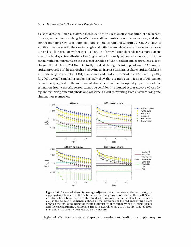
24 • Uncertainties in Ocean Colour Remote Sensing
a closer distance. Such a distance increases with the radiometric resolution of the sensor.
Notably, at the blue wavelengths AEs show a slight sensitivity on the water type, and they
are negative for green vegetation and bare soil (Bulgarelli and Zibordi 2018a). AE shows a
significant increase with the viewing angle and with the Sun elevation, and a dependence on
Sun and satellite position with respect to land. The former (latter) dependence is more evident
when the land spectral albedo is low (high). AE additionally evidences a noteworthy intra-
annual variation, correlated to the seasonal variation of Sun elevation and spectral land albedo
(Bulgarelli and Zibordi 2018b). It is finally recalled the significant dependence of AEs on the
optical properties of the atmosphere, showing an increase with atmospheric optical thickness
and scale height (Tanré et al. 1981; Reinersman and Carder 1995; Santer and Schmechtig 2000;
Sei 2007). Overall simulation results strikingly show that accurate quantification of AEs cannot
be universally applied on the sole basis of atmospheric and marine optical properties, and that
estimation from a specific region cannot be confidently assumed representative of AEs for
regions exhibiting different albedo and coastline, as well as resulting from diverse viewing and
illumination geometries.
Figure 3.6 Values of absolute average adjacency contributions at the sensor (ξLtot=Ladj/Ltot ) as a function of the distance from a straight coast oriented in the North-Southdirection. Error bars represent the standard deviation. Ltot is the TOA total radiance.Ladj is the adjacency radiance, defined as the difference in the radiance at the sensorbetween the case accounting for the non-uniformity of the underlying reflecting surfaceand the case assuming a uniform surface (Bulgarelli et al. 2014). Figure adapted fromBulgarelli et al. (2014) under the CC BY 4.0 license.
Neglected AEs become source of spectral perturbations, leading in complex ways to
Sources of Uncertainties • 25
uncertainties in derived products. Notably, for an atmospheric correction scheme inferring the
aerosol properties from NIR data, perturbations induced by AE at NIR and visible wavelengths
might compensate each other. As a consequence, biases induced by AE on radiometric
products (e.g., Lw ) are not strictly correlated to the intensity of the reflectance of the nearby
land. Theoretical estimates for an AC scheme determining the atmospheric properties from
the NIR region through a power-law spectral extrapolation indicated that percentage over- and
underestimates of the water-leaving radiance from Case-2 moderately sediment-dominated
waters might well exceed 100% at 443 nm at the coast in the presence of snow and green
vegetation, respectively, while misestimates might increase about 4 times for CDOM-dominated
waters (Bulgarelli and Zibordi 2018a). A validation exercise performed with SeaDAS (l2gen AC)
on a sample of cloud-free SeaWiFS images acquired at the AAOT site, and alternatively ingesting
original SeaWiFS data and SeaWiFS TOA data corrected for estimated adjacency contributions,
indicated a significant decrease of annual and intra-annual biases at all wavelengths when
correcting for AE (Bulgarelli et al. 2018). It is also true that the impact of AE on OC algorithm
outputs will vary with the characteristics of the algorithm.
Most proposed methods for the operational correction of AE in satellite images of water
bodies impose restrictions on sensor characteristics and specifications (e.g., Reinersman and
Carder 1995; Guanter et al. 2010; Sei 2015; Sterckx et al. 2015). A recent sensor independent
operational algorithm (Heege et al. 2014), implementing an analytical approximation of the
point-spread function for an arbitrary stratified atmosphere (Kiselev et al. 2015), allows
accounting for the actual angle of observation and coastal morphology. Empirical corrections
accounting for these variable factors can also be achieved through establishing look-up-tables
(LUTs) and processing each individual scene twice (Feng and Hu 2017). These developments
suggest that uncertainties due to land adjacency could be better characterized and reduced in
the future.
3.2.3 Sea Surface
Since the specular reflectance of direct Sun and scattered sky light at the air/sea interface
contributes to the path radiance, it has to be included in the atmospheric correction procedure.
Problems arise when Sun light is directly reflected to the sensor (Sun glint). Dependent on the
Sun and viewing angle and on the wave slope distribution, Sun glint may exceed by far the
water-leaving radiance and atmospheric path radiance. In standard ACs (e.g., l2gen in SeaDAS),
glint radiance is traditionally computed as a function of wind speed following Cox and Munk
(1954). Besides uncertainties on wind itself (Section 3.1.2), there are uncertainties on the
relationship between wind and wave surface-slope distributions. Again, wave distributions also
depend on swell and not only on local wind (Hanley et al. 2010). Additionally, AC algorithms
do not differentiate the effect of wind direction on sea surface roughness, which is incorrect
and may affect the determination of glint intensity. This being said, even though developed
60 years ago, the Cox and Munk parameterization appears to perform satisfactorily (Zhang
and Wang 2010; but see Hu et al. 2008 or Mobley 2015). In conditions deemed of high glint,
pixels are excluded from further processing in most AC schemes (with an appropriate flag)
26 • Uncertainties in Ocean Colour Remote Sensing
leading to potentially large losses of data, while an attempt at correcting for glint radiance
can be performed in moderate glint conditions (Wang and Bailey 2001). From Figure 3.2, the
average contributions from glint to the TOA radiance budget appear small but it is specific to
the geometries encountered as a function of latitude with SeaWiFS (a sensor operating with a
tilt to minimize Sun glint, Gregg and Patt 1994) and limited by the exclusion of situations of
high glint. Differently, some ACs process data in a wider range of glint conditions (Steinmetz
et al. 2011).
Whitecaps (sea foam) are another contributor to the TOA radiance budget. Traditionally,
radiance associated with whitecaps is modelled as a function of wind speed through its action
on whitecap fraction (Stramska and Petelski 2003). Uncertainties are associated with this
scheme since a large variability is observed among relationships between wind and whitecap
fraction (Anguelova and Webster 2006; Brumer et al. 2017); moreover, such relationships
usually ignore the secondary factor of wind history: for instance, sea state may be different
for increasing or decreasing winds (Callaghan et al. 2008). In a model study, Gordon and
Wang (1994a) suggested that whitecap modelling with a spectrally flat whitecap reflectance
was sufficiently accurate for wind speeds lower than 10–12 m s−1 in clear atmospheres; later
on, the decrease of whitecap reflectance towards the NIR has been shown, which might have a
potential impact on atmospheric correction (Frouin et al. 1996; Moore et al. 1998; Dierssen
2019). In the range of wind speed 9–12 m s−1, Moore et al. (2000) documented reflectance (here
defined as the ratio of upwelling radiance and above-water downwelling irradiance multiplied
by π ) of 0.001–0.002 with negligible contribution below 4 m s−1. Of course, strong winds are
often associated with storms and cloudy conditions but this is not general. Although fairly
small (see also Figure 3.2), these contributions might be relevant, again particularly in the
NIR, and improvements to better represent the whitecap radiance term would be certainly
helpful for atmospheric correction and for issues related with air-sea exchange. An area where
such progress would be particularly needed is the Southern Ocean, leading to an improved
distinction between the contribution to relatively high reflectance values from the local high
wind regime and that from the fields of coccolithophores creating a so-called calcite belt in
the region (Balch et al. 2011). It is finally noted that wind is not the only factor generating sea
foam: ship wakes can have a local impact on ocean brightness (Gatabe et al. 2011) that might
be relevant for high resolution imagery.
Besides specular reflectance and white caps, other phenomena can change the nature of the
atmosphere-ocean boundary and be particularly difficult to model or even detect. This might
be the case in polar regions where the presence of sea ice with various states of overlying snow
can impact the OC signal within the pixel (Bélanger et al. 2007; Perovich and Polashenski 2012).
Floating macro-algae such as Sargassum (Gower et al. 2006; Qi et al. 2017a) and Ulva (Hu
et al. 2017), the results of intense algal blooms in the form of surface scums or mats (Kutser
2004; Hu et al. 2010), mucilage or coccoliths (Gordon et al. 2001), or chemical phenomena
such as sulphur plumes (Weeks et al. 2004) are also conditions that standard algorithms are
usually not well prepared to handle. A further limit is set by the solar zenith angle. At low Sun
elevations some of the problems mentioned above increase, in particular those associated with
the transmittance through the atmosphere, the path radiance and the reflection at the surface.
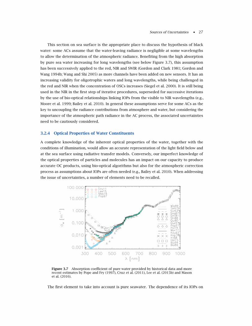
Sources of Uncertainties • 27
This section on sea surface is the appropriate place to discuss the hypothesis of black
water: some ACs assume that the water-leaving radiance is negligible at some wavelengths
to allow the determination of the atmospheric radiance. Benefiting from the high absorption
by pure sea water increasing for long wavelengths (see below Figure 3.7), this assumption
has been successively applied to the red, NIR and SWIR (Gordon and Clark 1981; Gordon and
Wang 1994b; Wang and Shi 2005) as more channels have been added on new sensors. It has an
increasing validity for oligotrophic waters and long wavelengths, while being challenged in
the red and NIR when the concentration of OSCs increases (Siegel et al. 2000). It is still being
used in the NIR in the first step of iterative procedures, superseded for successive iterations
by the use of bio-optical relationships linking IOPs from the visible to NIR wavelengths (e.g.,
Moore et al. 1999; Bailey et al. 2010). In general these assumptions serve for some ACs as the
key to uncoupling the radiance contributions from atmosphere and water, but considering the
importance of the atmospheric path radiance in the AC process, the associated uncertainties
need to be cautiously considered.
3.2.4 Optical Properties of Water Constituents
A complete knowledge of the inherent optical properties of the water, together with the
conditions of illumination, would allow an accurate representation of the light field below and
at the sea surface using radiative transfer models. Conversely, our imperfect knowledge of
the optical properties of particles and molecules has an impact on our capacity to produce
accurate OC products, using bio-optical algorithms but also for the atmospheric correction
process as assumptions about IOPs are often needed (e.g., Bailey et al. 2010). When addressing
the issue of uncertainties, a number of elements need to be recalled.
Figure 3.7 Absorption coefficient of pure water provided by historical data and morerecent estimates by Pope and Fry (1997), Cruz et al. (2011), Lee et al. (2015b) and Masonet al. (2016).
The first element to take into account is pure seawater. The dependence of its IOPs on
28 • Uncertainties in Ocean Colour Remote Sensing
temperature and salinity has been introduced in Section 3.1.2. Scattering by pure seawater is
now well known with strong theoretical underpinning (Zhang and Hu 2009). Much progress has
been made on the determination of absorption properties but uncertainties remain associated
with observational protocols applied to pure water. In the course of time, different absorption
spectra aw have been proposed as illustrated by Figure 3.7 that highlights some recent
determinations upon a historical background. The observed differences may come from
differences in measurement methodology as well as the means employed to obtain a “pure”
water sample. Logically, relative uncertainties are found higher where aw is lower, in the blue
to ultra-violet parts of the spectrum, and below 400 nm large differences still appear between
recent estimates. Mason et al. (2016) provide uncertainty estimates in association with their
aw values, of the order of 3% in the green bands, to ∼10% at 400–420 nm, up to >30% around
350 nm. Higher uncertainties in the lower range of aw values mean that they usually have a
small impact across the visible range when the total absorption budget is considered, but they
might not be negligible. Indeed, Figure 3.8 shows that for standard oligotrophic waters (see
figure caption), aw can weigh half of the total absorption in blue wavelengths.
By the additive principle, total IOPs are the sum of the IOPs associated with a myriad
of constituents found in the water, while in turn these are the results of optical properties
associated with each particle and dissolved samples. Our current capacity to model the
optical properties of natural waters is hampered by some serious issues that ultimately imply
uncertainties in any optical treatment. First of all, there is still ample room for progress to
thoroughly describe how observed IOPs are attributable to specific constituents in natural
waters. For instance, the relative contribution to backscattering bb by constituents with size
covering orders of magnitude (from colloids to zooplankton, dust and bubbles) is not fully
mastered (Stramski et al. 2004). Colloidal material in the size range 1 nm – 1 µm could be
a significant contributor to bb (Stramski and Wozniak 2005 but see Organelli et al. 2018)
and is still insufficiently characterized. A compounding factor is that a relevant part of the
colloids goes through the filters typically used to distinguish the dissolved and particulate
parts found in water. Beyond these operational limitations, representing the optical properties
of well-identified hydrosols is not a straightforward task. As for aerosols, some hydrosols do
not easily lend themselves to calculations of their optical properties using Mie theory, because
of their varied shapes and contents or as chain-forming organisms (e.g., Kirk 1976; Volten
et al. 1998; Clavano et al. 2007; Matthews and Bernard 2013) but progress is underway as
observations of individual particles and modelling techniques improve (e.g., Quirantes and
Bernard 2006; Olson and Sosik 2007; Moutier et al. 2016; Organelli et al. 2018). Still on the
issue of scattering, our main source of reference for measured scattering phase functions in
natural waters has been Petzold (1972) for a long time. Several studies have illustrated the
sensitivity of modelled AOPs to the choice of hydrosol scattering phase function (Mobley et al.
2002; Bulgarelli et al. 2003b; Tonizzo et al. 2017, Section 3.2.7) so that current progress in the
field (e.g., Chami et al. 2006; Berthon et al. 2007; Robertson-Lain et al. 2017) is much needed
for an improved representation of water optical properties.
A word is also due about inelastic processes, Raman scattering and fluorescence by CDOM
and phytoplankton. These phenomena can have a significant impact on the light field, including
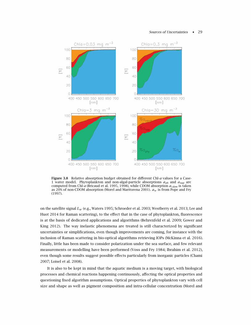
Sources of Uncertainties • 29
Figure 3.8 Relative absorption budget obtained for different Chl-a values for a Case-1 water model. Phytoplankton and non-algal-particle absorptions aph and anap arecomputed from Chl-a (Bricaud et al. 1995, 1998), while CDOM absorption acdom is takenas 20% of non-CDOM absorption (Morel and Maritorena 2001). aw is from Pope and Fry(1997).
on the satellite signal Lw (e.g., Waters 1995; Schroeder et al. 2003; Westberry et al. 2013; Lee and
Huot 2014 for Raman scattering), to the effect that in the case of phytoplankton, fluorescence
is at the basis of dedicated applications and algorithms (Behrenfeld et al. 2009; Gower and
King 2012). The way inelastic phenomena are treated is still characterized by significant
uncertainties or simplifications, even though improvements are coming, for instance with the
inclusion of Raman scattering in bio-optical algorithms retrieving IOPs (McKinna et al. 2016).
Finally, little has been made to consider polarization under the sea surface, and few relevant
measurements or modelling have been performed (Voss and Fry 1984; Ibrahim et al. 2012),
even though some results suggest possible effects particularly from inorganic particles (Chami
2007; Loisel et al. 2008).
It is also to be kept in mind that the aquatic medium is a moving target, with biological
processes and chemical reactions happening continuously, affecting the optical properties and
questioning fixed algorithm assumptions. Optical properties of phytoplankton vary with cell
size and shape as well as pigment composition and intra-cellular concentration (Morel and
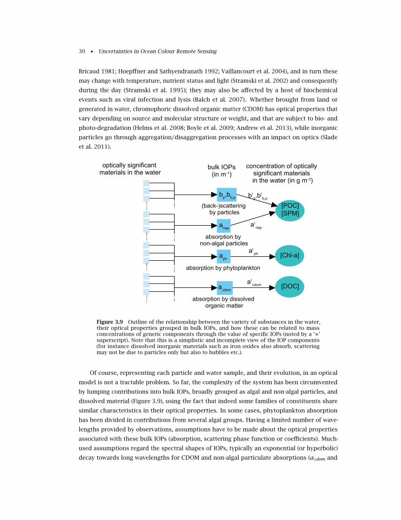
30 • Uncertainties in Ocean Colour Remote Sensing
Bricaud 1981; Hoepffner and Sathyendranath 1992; Vaillancourt et al. 2004), and in turn these
may change with temperature, nutrient status and light (Stramski et al. 2002) and consequently
during the day (Stramski et al. 1995); they may also be affected by a host of biochemical
events such as viral infection and lysis (Balch et al. 2007). Whether brought from land or
generated in water, chromophoric dissolved organic matter (CDOM) has optical properties that
vary depending on source and molecular structure or weight, and that are subject to bio- and
photo-degradation (Helms et al. 2008; Boyle et al. 2009; Andrew et al. 2013), while inorganic
particles go through aggregation/disaggregation processes with an impact on optics (Slade
et al. 2011).
! !
!
!
!
Figure 3.9 Outline of the relationship between the variety of substances in the water,their optical properties grouped in bulk IOPs, and how these can be related to massconcentrations of generic components through the value of specific IOPs (noted by a ‘∗’superscript). Note that this is a simplistic and incomplete view of the IOP components(for instance dissolved inorganic materials such as iron oxides also absorb, scatteringmay not be due to particles only but also to bubbles etc.).
Of course, representing each particle and water sample, and their evolution, in an optical
model is not a tractable problem. So far, the complexity of the system has been circumvented
by lumping contributions into bulk IOPs, broadly grouped as algal and non-algal particles, and
dissolved material (Figure 3.9), using the fact that indeed some families of constituents share
similar characteristics in their optical properties. In some cases, phytoplankton absorption
has been divided in contributions from several algal groups. Having a limited number of wave-
lengths provided by observations, assumptions have to be made about the optical properties
associated with these bulk IOPs (absorption, scattering phase function or coefficients). Much-
used assumptions regard the spectral shapes of IOPs, typically an exponential (or hyperbolic)
decay towards long wavelengths for CDOM and non-algal particulate absorptions (acdom and
Sources of Uncertainties • 31
anap , respectively), and a power law for particulate back-scattering (bbp), while phytoplankton
absorption (aph amplitude and spectral shape) and scattering have often been parameterized
as a function of Chl-a (e.g., Bricaud et al. 1995; Loisel and Morel 1998). Literature abounds with
descriptions of specific parameterizations for the various constituents (see example reviews
in Blough and Del Vecchio 2002; Twardowski et al. 2004; Berthon et al. 2008; Werdell et al.
2018). For oceanic waters, under the assumption that all optical properties are ultimately
driven by phytoplankton, the so-called Case-1 model allows the determination of all IOPs as a
function of Chl-a (Morel and Maritorena 2001) but significant variations around that model
are actually observed. Even though the assumptions employed in ocean optics have allowed
remarkable results, there is no ignoring that they also introduce uncertainties that cannot
easily be reduced. The importance of these uncertainties obviously depends on the weight
that a component IOP has in the overall absorption/scattering budget; conversely the capacity
to discriminate a given component also depends on this weight. Figure 3.8 shows relative
absorption budgets across a Chl-a gradient, with different contributions depending on Chl-a
and wavelength within a Case-1 water framework. Other water types typically found in coastal
regions and marginal seas may show different results (Berthon et al. 2008); in some extreme
cases, a component IOP can be completely obscured by the others (for instance phytoplankton
in very absorbing waters), putting severe limitations on the level of uncertainties that can be
achieved for this specific component.
IOPs are often used as intermediary products to compute concentrations of optically signi-
ficant constituents (OSC), such as Chl-a (through aph), suspended particulate matter (SPM, for
instance through attenuation due to particles cp , bbp or anap), particulate organic carbon (POC,
through cp or bbp) or dissolved organic carbon (DOC, through acdom) (Figure 3.9), by writing
that IOP and concentration [C] can be linked by IOP=IOP∗ ×[C], where IOP∗ is called a specific
IOP (sIOP, in m2 g−1) and is assumed known. Because of the same complexity characterizing
hydrosols and their medium described above, sIOPs vary according to a host of factors, again
being related to sources, chemical compositions, biological status, etc. (Neukermans et al.
2012a), and cover significant intervals of variability (example review in Zheng and DiGiacomo
2017).
Figure 3.10 shows the example of the relationship between aph at 443 nm and Chl-a
obtained using the NASA bio-Optical Marine Algorithm Data set (NOMAD, Werdell and Bailey
2005) for open ocean waters (loosely defined by a bottom depth larger than 100 m). Even
though a linear regression (performed on log-transformed data) performs reasonably well, a
significant dispersion is still seen, in line with other studies (e.g., Bricaud et al. 1998) or with
results obtained for back-scattering versus Chl-a (Huot et al. 2008). Again, this variability can
be explained by different cell sizes and pigment compositions. Both absorptions by CDOM and
non-algal particles can be well represented by an exponential (or hyperbolic) decay towards
long wavelengths, with exponential slopes found in similar ranges, which makes it hard to
separate the two contributions and often leads to considering a bulk absorption acdm for
coloured detrital material (CDM) proportional to exp(-Sλ). The slope S varies significantly
in natural waters, typically in the range 0.01–0.02 nm−1 (see Blough and Del Vecchio 2002;
Twardowski et al. 2004 for CDOM) even though part of this variability comes from the spectral
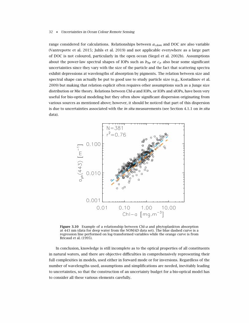
32 • Uncertainties in Ocean Colour Remote Sensing
range considered for calculations. Relationships between acdom and DOC are also variable
(Vantrepotte et al. 2015; Juhls et al. 2019) and not applicable everywhere as a large part
of DOC is not coloured, particularly in the open ocean (Siegel et al. 2002b). Assumptions
about the power-law spectral shapes of IOPs such as bbp or cp also bear some significant
uncertainties since they vary with the size of the particle and the fact that scattering spectra
exhibit depressions at wavelengths of absorption by pigments. The relation between size and
spectral shape can actually be put to good use to study particle size (e.g., Kostadinov et al.
2009) but making that relation explicit often requires other assumptions such as a Junge size
distribution or Mie theory. Relations between Chl-a and IOPs, or IOPs and sIOPs, have been very
useful for bio-optical modeling but they often show significant dispersion originating from
various sources as mentioned above; however, it should be noticed that part of this dispersion
is due to uncertainties associated with the in situ measurements (see Section 4.1.1 on in situ
data).
Figure 3.10 Example of a relationship between Chl-a and phytoplankton absorptionat 443 nm (data for deep water from the NOMAD data set). The blue dashed curve is aregression line performed on log-transformed variables while the orange curve is fromBricaud et al. (1995).
In conclusion, knowledge is still incomplete as to the optical properties of all constituents
in natural waters, and there are objective difficulties in comprehensively representing their
full complexities in models, used either in forward mode or for inversions. Regardless of the
number of wavelengths used, assumptions and simplifications are needed, inevitably leading
to uncertainties, so that the construction of an uncertainty budget for a bio-optical model has
to consider all these various elements carefully.
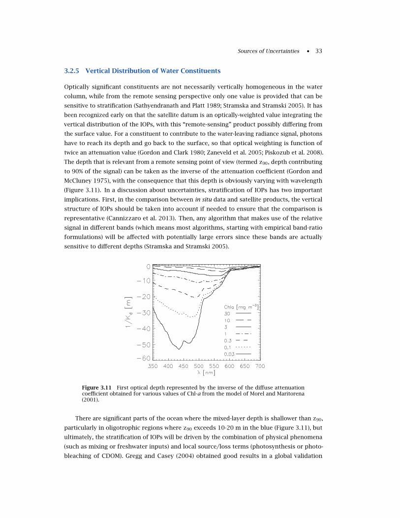
Sources of Uncertainties • 33
3.2.5 Vertical Distribution of Water Constituents
Optically significant constituents are not necessarily vertically homogeneous in the water
column, while from the remote sensing perspective only one value is provided that can be
sensitive to stratification (Sathyendranath and Platt 1989; Stramska and Stramski 2005). It has
been recognized early on that the satellite datum is an optically-weighted value integrating the
vertical distribution of the IOPs, with this “remote-sensing” product possibly differing from
the surface value. For a constituent to contribute to the water-leaving radiance signal, photons
have to reach its depth and go back to the surface, so that optical weighting is function of
twice an attenuation value (Gordon and Clark 1980; Zaneveld et al. 2005; Piskozub et al. 2008).
The depth that is relevant from a remote sensing point of view (termed z90, depth contributing
to 90% of the signal) can be taken as the inverse of the attenuation coefficient (Gordon and
McCluney 1975), with the consequence that this depth is obviously varying with wavelength
(Figure 3.11). In a discussion about uncertainties, stratification of IOPs has two important
implications. First, in the comparison between in situ data and satellite products, the vertical
structure of IOPs should be taken into account if needed to ensure that the comparison is
representative (Cannizzaro et al. 2013). Then, any algorithm that makes use of the relative
signal in different bands (which means most algorithms, starting with empirical band-ratio
formulations) will be affected with potentially large errors since these bands are actually
sensitive to different depths (Stramska and Stramski 2005).
Figure 3.11 First optical depth represented by the inverse of the diffuse attenuationcoefficient obtained for various values of Chl-a from the model of Morel and Maritorena(2001).
There are significant parts of the ocean where the mixed-layer depth is shallower than z90,
particularly in oligotrophic regions where z90 exceeds 10-20 m in the blue (Figure 3.11), but
ultimately, the stratification of IOPs will be driven by the combination of physical phenomena
(such as mixing or freshwater inputs) and local source/loss terms (photosynthesis or photo-
bleaching of CDOM). Gregg and Casey (2004) obtained good results in a global validation
34 • Uncertainties in Ocean Colour Remote Sensing
of SeaWiFS Chl-a product without accounting for possible stratification; nonetheless the
vertical structure of IOPs should be considered as completely as possible to reduce the
related uncertainties. The vertical structure of Chl-a has been already well documented
(Sathyendranath et al. 1995; Uitz et al. 2006) but more knowledge is forthcoming with new
systems such as the BioArgo floats (Sauzède et al. 2016).
3.2.6 Effects of the Bottom
In optically shallow water, defined with bottom depths shallower than the inverse of the
attenuation coefficient, the reflection of Sun light by the bottom can contribute to the water-
leaving radiance. Most algorithms do not take this effect into account. Then, in a strict sense,
such a condition is out of range of the algorithm and causes uncertainty in the retrieval of
IOPs or concentration of water constituents (Bulgarelli et al. 2003b). Since the attenuation
coefficient is wavelength dependent, some of the spectral bands might be affected by bottom
reflection while others are not. In clear water these might be the blue spectral bands, while in
turbid water the green bands might be affected. A correction for bottom effects is challenging
because of the difficulty in disentangling the optical effects of the water column, with its depth
and IOPs, and of the bottom, with its own bidirectional reflectance function, heterogeneity and
slope (e.g., Philpot et al. 2004). The potential increase in re-suspended particles close to the
bottom is a further complicating factor. Corollaries are that hyperspectral data are required to
address this complex problem but that in proper conditions OC data can provide information
on bathymetry and bottom types with acceptable uncertainties (Dierssen et al. 2003; Mobley
et al. 2005).
3.2.7 Relation Between IOPs and AOPs and Bi-directional Effects
AOPs can be expressed as a function of IOPs (and geometry of observation/illumination)
(Zaneveld 1995); this has led to the writing of analytic expressions linking RRS or LW to IOPs
to be used in inverse mode for the retrieval of the latter. At that point it is worth writing the
relationship linking the various quantities of relevance, where the remote sensing reflectance
RRS is:
RRS(θ, θ0,φ) =Lw(θ, θ0,φ)Ed(0+, θ0)
= (1− ρ)(1− ρ)(1− rR)n2
w
R(θ0)Q(θ, θ0,φ)
(3.2)
where Lw is the water-leaving radiance (just above the sea surface, at 0+) observed with the
geometry defined by viewing and solar zenith angles θ and θ0, respectively, and relative
azimuth φ, Ed(0+) is the downwelling irradiance at 0+, R is the ratio of downwelling and
upwelling irradiance just below the surface (0−) and Q is the ratio of upwelling irradiance
and radiance at 0−. Lw is linked to the upwelling radiance just below the water surface,
Lu(0−), by Lw(θ, θ0,φ) = 1−ρ(θ)n2wL−u(θ, θ0,φ) (see Gordon and Voss 2018 for discussion). The
first ratio on the right-hand side of Equation 3.2 contains several non-dimensional quantities
that represent the relevant refraction/reflection effects through the air-water interface: ρ the
air-water Fresnel reflection for Sun+sky downwelling irradiance (typically around 4-5%), ρ the
Sources of Uncertainties • 35
internal Fresnel reflectance (∼0.02 for θ=0 and a flat ocean but depending on the surface state
often parameterized by wind speed), r the water-air reflectance for totally diffuse upwelling
irradiance (often approximated as 0.48-0.49), nw the index of refraction of water. Noted as
a Gothic < by Morel and Gentili (1996), this term still depends on the irradiance reflectance
R. Some of its components are well constrained (Morel and Gentili 1996): 1-ρ is ∼0.957,
±3% depending on atmospheric conditions and solar elevation (Gordon et al. 1988b), 1-rR is
∼0.985, ±1.5% if R is between 0 and 0.06, and nw is ∼1.341 (weakly depending on wavelength,
temperature and salinity, Austin and Halikas 1972). The term < has been modeled as a
function of θ and wind speed (in relation with ρ), but actually the dependence on wind is
very small for speeds up to 20 m s−1 (Gordon 2005) where anyway issues with white caps
become important (see Section 3.2.3). The use of look-up tables for < (Morel et al. 2002, with
correction following Gordon 2005) or assumptions such as (1-ρ)(1-ρ)/n2w ∼0.52-0.54 (Lee et al.
2002) allow a direct link between above- and below-water quantities with a certain degree
of confidence. However, the wavy character of the sea surface has significant effects on the
in-water light field (e.g., D’Alimonte et al. 2010; Hieronymi and Macke 2012) and how these
scale up to the size of a satellite pixel may not be fully well parameterized. Additionally, the
complexity of the interactions between wave distribution and wind field (selected as a predictor
variable because easily available from models or remote sensing) and the importance of swell
(Hanley et al. 2010) make relationships between wave and wind imperfect.
The radiance field in natural waters (represented by below-water radiance Lu) is usually
not isotropic (Morel and Gentili 1993) with the bidirectional reflectance distribution function
(BRDF) of Lu varying with water IOPs (e.g., Loisel and Morel 2001; Zibordi and Berthon 2001;
Chang et al. 2007; Zhai et al. 2015). That makes the construction of relationships between
AOPs and IOPs particularly challenging. Starting with Gordon and Clark (1981), notations
have been introduced leading to the definition of the normalized water-leaving radiance, the
radiance LWN that would be observed with a nadir view and the Sun at zenith, in the absence
of atmosphere and with the Sun at the mean Earth-Sun distance:
Lw(θ, θ0,φ) =(dd
)2
cosθ0td,s(θ0)<(θ, θ0,φ)<(0)
R(θ0)R(0)
Q(0)Q(θ, θ0,φ)
LWN (3.3)
Lw(θ, θ0,φ) =(dd
)2
cosθ0td,s(θ0)<(θ, θ0,φ)<(0)
f (θ0)Q(θ, θ0,φ)
Q(0)f (0)
LWN (3.4)
with td,s the diffuse transmittance (from Sun to surface) and d the Earth-Sun distance (with
d being its mean value). In the form of Equation 3.4, the quantity f has been introduced as
defined by R=f bb/a, linking IOPs and AOPs (Morel and Prieur 1977). The conversion in LWN(or an equivalent RRS ) is particularly relevant as it allows a direct comparison (i.e., with the
same, idealized, conditions of measurement) between data from different satellite missions as
well as with field data, but this process is affected by uncertainties.
In that step, there is an uncertainty associated with the transmittance term that is related
to the atmospheric correction process (see Section 3.2.1). The main issue here is the represen-
tation of the bidirectional nature of the upwelling radiance field in Equations 3.2 to 3.4 (but it
36 • Uncertainties in Ocean Colour Remote Sensing
might be noticed that the BRDF has a secondary effect on td itself, Gordon and Franz 2008).
One limitation on this topic is that relevant in situ data sets, necessitating measurements of
Lu in various geometries, are not common (Tyler 1960; Voss and Chupin 2005; Lewis et al.
2011; Antoine et al. 2013), which partly explains that models of Q or f/Q usually rely on
radiative transfer simulations (Morel et al. 2002; Park and Ruddick 2005; Lee et al. 2011; Hlaing
et al. 2012; Fan et al. 2016) and that validation exercises are few. These show satisfactory
agreements for parameterizations developed for open ocean waters (within a Case-1-water
framework, Morel et al. 2002), with differences between model results and observations within
the uncertainties of the measurements (Morel et al. 1995; Voss et al. 2007), or differences
of ∼7% in Baja California waters (Voss and Morel 2005). Other comparisons show levels of
differences that vary with water types and methods (Lee et al. 2011; Gleason et al. 2012; Fan
et al. 2016; Talone et al. 2018). Published numbers are still significant enough to weigh in un-
certainty budget for LWN and derived IOPs and warrant more developments and observations.
It is worth stressing that a straightforward expression of the BRDF effects actually implies a
knowledge of the in-water IOPs, which is the point of solving the inversion of LWN or RRS in
the first place. It must be kept in mind that the operation of bio-optical algorithms and the
issue of the BRDF effects and the related uncertainties are obviously coupled.
AOPs/IOPs relationships are at the basis of a suite of algorithms, with typically rrs , below-
water remote sensing reflectance, written as simple functions of backscattering and absorption
ratios, bb/a or bb/(bb + a), for instance:
rrs(θ, θ0,φ) =R(θ0)
Q(θ, θ0,φ)= f(θ0)Q(θ, θ0,φ)
bba= f ′(θ0)Q(θ, θ0,φ)
bbbb + a
(3.5)
rrs(θ, θ0,φ) =R(θ0)
Q(θ, θ0,φ)= g0
bbbb + a
+ g1
(bb
bb + a
)2
(3.6)
The first IOP expression (Equation 3.5) follows the work by Morel and co-workers (e.g., Morel
et al. 2002), where the function f (see above) or equivalently f ′, was parameterized as a
function of θ0 and Chl-a as synonymous with all IOPs in a Case-1-water framework. In that
case, Q or the ratio f/Q can be stored in look-up tables (LUTs) that are functions of Chl-a and
geometry, allowing a direct link between rrs and Chl-a. The second IOP expression (Equation
3.6) posits that rrs can be approximated by a second-order polynomial with g0 and g1 constant
(for example, 0.0949 and 0.0794, respectively, for θ=0 and θ0 > 20◦ in Gordon et al. 1988b).
Both cases are therefore characterized by strong hypotheses with assumptions about the
water content or at least about some optical properties leading to simplifications such as the
two-degree polynomial form. More complex formula have been proposed (Albert and Mobley
2003; Park and Ruddick 2005; Van der Woerd and Pasterkamp 2008; Lee et al. 2011) but all
algorithms based on analytical formalisms linking IOPs and AOPs such as those of Equations
3.5 or 3.6 rely to some extent on some assumptions (particularly about the scattering phase
functions of the water) that are sources of uncertainties.
Optical closure experiments, aiming at reaching consistency between IOPs and radiometry,
are efficient benchmarks to assess the accuracy of field measurements together with our capa-
city to model the optical properties of the medium. Considering the sources of uncertainties
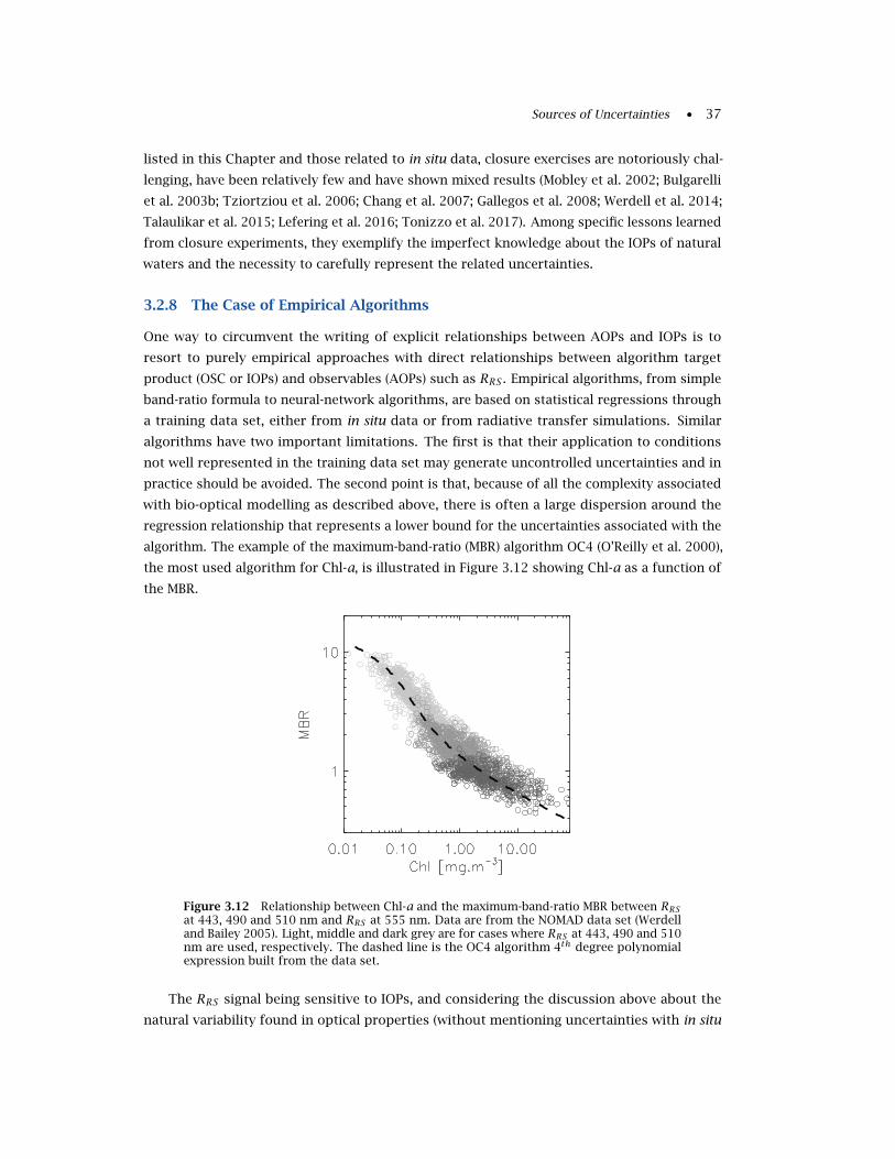
Sources of Uncertainties • 37
listed in this Chapter and those related to in situ data, closure exercises are notoriously chal-
lenging, have been relatively few and have shown mixed results (Mobley et al. 2002; Bulgarelli
et al. 2003b; Tziortziou et al. 2006; Chang et al. 2007; Gallegos et al. 2008; Werdell et al. 2014;
Talaulikar et al. 2015; Lefering et al. 2016; Tonizzo et al. 2017). Among specific lessons learned
from closure experiments, they exemplify the imperfect knowledge about the IOPs of natural
waters and the necessity to carefully represent the related uncertainties.
3.2.8 The Case of Empirical Algorithms
One way to circumvent the writing of explicit relationships between AOPs and IOPs is to
resort to purely empirical approaches with direct relationships between algorithm target
product (OSC or IOPs) and observables (AOPs) such as RRS . Empirical algorithms, from simple
band-ratio formula to neural-network algorithms, are based on statistical regressions through
a training data set, either from in situ data or from radiative transfer simulations. Similar
algorithms have two important limitations. The first is that their application to conditions
not well represented in the training data set may generate uncontrolled uncertainties and in
practice should be avoided. The second point is that, because of all the complexity associated
with bio-optical modelling as described above, there is often a large dispersion around the
regression relationship that represents a lower bound for the uncertainties associated with the
algorithm. The example of the maximum-band-ratio (MBR) algorithm OC4 (O’Reilly et al. 2000),
the most used algorithm for Chl-a, is illustrated in Figure 3.12 showing Chl-a as a function of
the MBR.
Figure 3.12 Relationship between Chl-a and the maximum-band-ratio MBR between RRSat 443, 490 and 510 nm and RRS at 555 nm. Data are from the NOMAD data set (Werdelland Bailey 2005). Light, middle and dark grey are for cases where RRS at 443, 490 and 510nm are used, respectively. The dashed line is the OC4 algorithm 4th degree polynomialexpression built from the data set.
The RRS signal being sensitive to IOPs, and considering the discussion above about the
natural variability found in optical properties (without mentioning uncertainties with in situ
38 • Uncertainties in Ocean Colour Remote Sensing
data), the dispersion around the regression line is not surprising. The residuals that can exceed
a factor of 2 have been related to variations between ocean basins and to variations in the
Chl-a-specific IOPs and weight of acdm in the absorption budget (Dierssen 2010; Szeto et al.
2011). The OC4 algorithm is particularly subject to this variability as it aims at covering the
global open ocean, but to various extents all empirical algorithms are confronted to the same
phenomena.
3.3 Uncertainties Associated with Data Editing
All the previous sections deal with uncertainties that affect a single pixel (i.e., from level-1
to level-2, Figure 3.3). But a vast share of ocean colour data applications rely on level-3 data,
where pixel-wise data are combined into gridded information for a specific amount of time. To
quantify how the uncertainties associated with these level-2 data propagate to level-3 products
is a complex step. Scott and Werdell (2019) have compared validation statistics obtained with
level-2 data and with daily level-3 data (with two different map projections). Statistics are
similar when common data are considered but may differ to some extent as more validation
points are identified for level-3 data, a fact explained by different match-ups selection protocols
(for instance, for level-3 products, a wider temporal window is allowed for the inclusion of in
situ data; see Section 4.1.2 for the presentation of validation protocols). The map projection
selected for level-3 data might also have an impact as variously distorting the location of the
original level-2 pixels (Scott and Werdell 2019).
To describe mathematically the transition from level-2 to level-3, it is worth adopting a
simple model that combines pixel-wise data by spatial averaging (which is actually at the core
of standard level-3 ocean colour data creation) or daily data into temporal composites. In that
case, the model output is:
y = 1N
N∑i=1
xi (3.7)
Before proceeding, it is worth mentioning that the statistical interpretation of the mean
(Equation 3.7) may require some assumptions on the data distribution function (typically
normality).
Applying uncertainty propagation as presented in Section 4.2.8 (Taylor expansion), the
standard (squared) uncertainty on y is:
u2(y) = 1N2
N∑i=1
N∑j=1
u(xi)u(xj)r(u(xi),u(xj)) (3.8)
considering the derivatives with respect to xi are all equal to 1/N , and r(u(xi),u(xj)) being
the error correlation between xi and xj . Equation 3.8 being written in terms of variance,
systematic effects are not included. By introducing an ‘average’, or representative, correlation
coefficient r between the errors in (xi)’s, the equation can be rewritten as:
Sources of Uncertainties • 39
u2(y) = 1N2
N∑i=1
N∑j=1
u(xi)u(xj)[δji + (1− δ
ji )r] (3.9)
where δji is the Kronecker δ (equal to 1 if i=j, 0 otherwise). The expression can be further
developed into:
u2(y) = 1− rN2
N∑i=1
u2(xi)+rN2
N∑i=1
u(xi)
2
(3.10)
From this, two extreme cases can be discussed. If all input errors are uncorrelated (r=0), the
expression becomes:
u(y) = 1√N
√√√√√ 1N
N∑i=1
u2(xi) (3.11)
with the well-known result that the uncertainty of the average is decreasing as a function of
1/√N for uncorrelated errors (again not considering systematic effects). To the opposite, if
the errors in (xi)’s are perfectly correlated (r=1),
u(y) = 1N
N∑i=1
u(xi) (3.12)
meaning that the output uncertainty is the average of the input uncertainties.
More thorough mathematical developments are available to treat that problem (it has been
well addressed for the combination of in situ point measurements into gridded products, e.g,
Morrissey and Greene 2009) but this simple development clearly illustrates one phenomenon
at play when building level-3 products: the standard uncertainty of the level-3 datum tends to
decrease with an increase in the number of input data at a pace defined by the error correlation
structure of the input data. Note that this is equally valid if data are combined in space or in
time. One case where input data errors are well correlated is when the uncertainty is dominated
by systematic effects rather than by random contributions.
Overall, combination of data tends to decrease the uncertainty of the aggregated data
(even though the process implies a loss of information, Pogson and Smith 2015) but this is
only one part of the picture. When creating a gridded product from pixel-based data, it is
possible that part of the associated surface be left uncovered as some pixels do not provide
valid retrievals (because of clouds or any other adverse conditions). This effect, that can be
termed sampling uncertainty, occurs when pixel data are binned into a grid cell, or when
grid cells are further combined into larger cells (for coarser resolutions) if some of them are
missing. The values of grid-box sampling uncertainty and large-scale sampling uncertainty
(following the wording of Kennedy 2014) tend to decrease when aggregating more data and to
increase for more variable data, particularly if the missing data are not randomly distributed
(see Bulgin et al. 2016 for the case of sea surface temperature). Ocean colour products are
impacted by all scales of variability found in the ocean (in relation to physical and biological
phenomena), from microscale turbulence and internal waves to sub-mesoscale and mesoscale
40 • Uncertainties in Ocean Colour Remote Sensing
structures (Franks 1997; Doney et al. 2003; Uz and Yoder 2004; Lévy et al. 2012) and the effect
of sampling will vary as a function of the prevalent conditions. Moses et al. (2016) suggest
that a large part of the variation in coastal areas is associated with scales below a few hundred
meters which is thus averaged out in kilometer-scale pixels. An improved representation of
spatial variability and covariance in ocean colour fields and related uncertainties will help in
addressing sampling uncertainties. New techniques (for instance using fractals, Skákala and
Smyth 2015) could help in that regard.
The same question is valid for temporal binning: in the transition from daily data to
weekly, monthly or seasonal composites, some components of product uncertainty tends
to decrease by averaging out (as per Equations 3.9 or 3.10) while the very process of data
binning introduces sampling uncertainty by inferring a time composite value from incomplete
information (Wiggert et al. 1994; Reuter et al. 2010). Composite (like monthly) OC products
usually rely on a sub-sample of days (Maritorena et al. 2010), to an extent that depends on
spatial resolution, a limitation particularly strong in cloudy regions (like at high latitudes) and
in general where atmospheric conditions are challenging for atmospheric correction (e.g., the
Arabian Sea during the summer monsoon). As for spatial binning, the sampling uncertainty
for temporal binning is higher in conditions of high variability, particularly if the missing data
are not evenly distributed in the considered time period. Managing cases with a significant
number of consecutive days with missing data is particularly challenging as phytoplankton
can evolve rapidly in some circumstances. Moreover, if, for any reason, conditions leading to
data exclusion (flagging) for the atmospheric correction (e.g., desert dust plumes) correlates to
some extent with specific conditions in the ocean, then time composites will end up biased.
The impact of missing days in time composites should not be underestimated: some studies
have shown that inter-mission comparison statistics are degraded when comparing monthly
averages with respect to daily values, particularly when the number of days is relatively low
(e.g., Barnes and Hu 2015). Gregg and Casey (2007) have quantified typical uncertainties
expected from sub-sampling using biogeochemical model outputs (see Section 4.2.14 for more
details).
So far, the transition from level-2 pixel-based data to gridded level-3 data has been
considered only from the point of view of spatial binning. The results of that process are
usually termed daily level-3 data, whereas the observations are mostly timed around local
noon (±3 hours) for polar-orbiting missions (but more satellite orbits overlap at high latitudes).
There is an uncertainty associated with that step as OC related quantities show diurnal
variability. High frequency (hours or less) changes have been documented for apparent and
inherent optical properties, in coastal waters or open ocean (e.g., Wiggert et al. 1999; Binder
and DuRand 2002; Chang et al. 2002; Mélin and Zibordi 2007; Kheireddine and Antoine 2014).
Diurnal changes have also been detected from remote sensing data (Shi et al. 2011; Wang et al.
2013; Arnone et al. 2017; Zhang et al. 2018) with geostationary missions bringing a precious
potential for this type of analysis. These variations are associated with biological phenomena
(in relation to physiological cycles of phytoplankton and zooplankton) and physical variability
(in association with vertical variations, tides, horizontal advection etc.). The “daily” satellite
product should not be assumed to be a 24-hour average, unless more work is performed to
Sources of Uncertainties • 41
quantify the associated uncertainty (that could very well include a bias).
Some work has been done to go beyond simple level-3 data and propose more complete
OC products using gap-filling techniques, for instance based on empirical orthogonal functions
or wavelets (Pottier et al. 2008; Sirjacobs et al. 2011). The development and operation of such
techniques will require some effort to include specific uncertainty propagation schemes.
In general, improvement is needed to compute and document the covariance of error fields
for OC products. Besides being an element required to properly characterize higher-level data,
it may also be distributed as a product in its own right and required for some applications
such as data assimilation. For example, Ford and Barciela (2017) did not use the uncertainty
values distributed with the OC products they selected for data assimilation because of an issue
of representativeness (with small scale processes captured by the observations not resolved
by the model). As similar difficulties are partly model-specific, a close collaboration with the
model community would be beneficial.
To conclude this section on higher-level products, it might be worth discussing the nature
of systematic and random contributions to uncertainties. In the context of a repetition of
measurements in fixed conditions in a laboratory, the distinction is clear. When considering
a given satellite image in natural conditions, this aspect is somewhat less clear-cut. The
uncertainties associated with each pixel are affected by noise from the top-of-atmosphere
data, and this contribution tends to decrease as a function of 1/√N as explained above. On
the other hand, remote sensing reflectance can be associated with systematic errors across
part or the whole of a scene, for instance because of the functioning of a specific camera
or a consistent response of the atmospheric correction in the presence of a certain type of
aerosols. However, this systematic contribution to uncertainties might only be local, in space
if another type of aerosols eliciting another response is found 100 kilometers away, or in
time if this type of aerosols is substituted by another type the day after or in the next season.
An implication is that the distribution of uncertainties in OC products might be significantly
influenced by scales of variability of atmospheric variables. By the same token systematic
differences between satellite products and in situ data that can be noticed during the time of
an oceanographic campaign (often called bias) might just disappear if a full seasonal cycle
is considered. Another implication is that the interpretation of validation statistics in terms
of mission-long properties needs to be done with caution as matchups might not be evenly
distributed in time and space. Time series of RRS have shown a seasonal cycle of the validation
statistics (Zibordi et al. 2012a) and inter-comparison analyses of several satellite missions have
also shown seasonal and spatial variability in inter-mission differences of apparent or inherent
optical properties (e.g., Zhang et al. 2006; Mélin et al. 2009, 2016; Djavidnia et al. 2010; Mélin
2010, 2011). On even longer time scales it is possible to observe a mission bias for a given
region, but a different bias may be found for a successive mission. Eventually, in the context
of Earth observation, the systematic contribution to an uncertainty budget is dependent on the
temporal and spatial scales considered. Finally, it is important to keep track of all sources of
uncertainties: systematic effects can appear fairly small in the first stages of the processing
with respect to total uncertainty, but they may become dominant and significant for higher
level products (averaged over large space and/or time scales) (Merchant et al. 2017).

42 • Uncertainties in Ocean Colour Remote Sensing
Chapter 4
Uncertainty Estimates
Frédéric Mélin, Emmanuel Boss, Robert J.W. Brewin, Roland Doerffer, Bryan A.
Franz, Robert Frouin, Martin Hieronymi, Chuanmin Hu, Thomas Jackson, Sylvain
Jay, Dominique Jolivet, Erdem M. Karaköylü, Hiroshi Kobayashi, Nicolas Lamquin,
Lachlan I.W. McKinna, Griet Neukermans and P. Jeremy Werdell
This Chapter is organized in three main sections. The first section focuses on the field measu-
rements that are so important to link observations from space to ground-based knowledge; it
describes how in situ data are used for validation purposes after a synthesic description of
the uncertainties affecting them. The second section is a review of the methods that, besides
validation with in situ data, have been used to estimate uncertainties associated with satellite
products. Finally, the state of knowledge on uncertainties affecting satellite products is briefly
reviewed.
4.1 Use of Field Observations
4.1.1 Uncertainties of Field Observations
In situ observations have a central and irreplaceable role in evaluating uncertainties of OC
remote sensing products. Besides the information they provide for the development of
algorithms, they have been extensively used for the purpose of validation, defined here as
the comparison between field values and satellite products. However, the interpretation of
validation results in term of uncertainties is not straightforward for two main reasons: i) in situ
data have their own uncertainties and ii) satellite and in situ data may be collected at different
times and different wavelengths (for spectral quantities) and they may differ in spatial scales,
leading to an issue of representativeness (or representation error, Oke and Sakov 2008). These
issues might contribute significantly to the differences observed between satellite and field
data and should be properly considered in validation exercises. Uncertainties of in situ data
are briefly addressed in the following sub-section. Then validation protocols and analysis are
discussed.
v Water-leaving Radiance / Remote Sensing Reflectance
Field data of radiometric quantities that are the primary OC products, water-leaving radiance
Lw or remote sensing reflectance RRS , are affected by various types of uncertainties related to
the instrument itself or its deployment and operation (Zibordi and Voss 2014). Uncertainties
43
44 • Uncertainties in Ocean Colour Remote Sensing
associated with field radiometers can be traced to calibration and some characteristics of the
instrument: straylight, out-of-band response, non-linear response, non-cosine response for
irradiance sensors (Zibordi and Bulgarelli 2007), immersion factor etc. In-water and above-
water measurements are further affected by their specific deployment conditions. The former,
conducted through radiometric profiles, may be affected by tilt, self-shading (Gordon and
Ding 1992; Zibordi and Ferrari 1995; Shang et al. 2017), the impact of waves (Zaneveld et al.
2001; Zibordi et al. 2004a; D’Alimonte et al. 2013), inelastic processes (Li et al. 2016), or
perturbations due to a deployment superstructure (Doyle and Zibordi 2002). A comprehensive
review of how 3-dimension radiative transfer modelling can contribute to estimating these
uncertainties is provided by Bulgarelli and D’Alimonte (2014). Measurements of radiative
properties on profiling floats have their own challenges with respect to uncertainty estimation
(see Gerbi et al. 2016 for a full accounting). Measurements collected in long deployments may
also suffer from bio-fouling. Above-water measurements are also affected by waves (regulating
the glint field, Zibordi et al. 2002b), the effect of sky-light polarization (Harmel et al. 2012)
or perturbations from a superstructure (a ship or a fixed structure, Hooker and Morel 2003;
Hooker and Zibordi 2005). Raw measurements may also need some further elaboration like
the correction for bidirectional effects to express the so-called normalized quantities (Section
3.2.7) or for inelastic processes (Section 3.2.4).
Considering that uncertainty requirements for satellite-derived Lw or RRS in the visible are
typically 5% (see Section 6.1), field data should comply with uncertainties at most equal to that
threshold. The few studies describing a full uncertainty budget for radiometric measurements
are interesting for the final results but also for the approach followed to identify the various
components contributing to the total uncertainty and to combine them. Uncertainty budgets
have been drawn for measurements from reference buoys (Brown et al. 2007; Antoine et al.
2008), fixed observing systems (Zibordi et al. 2004b), autonomous profiling systems (Gerbi et al.
2016), or some oceanographic campaigns (Hooker et al. 2004). Uncertainty estimates are often
provided in relative values (%) but uncertainties in radiometric units have also been provided
(Deschamps et al. 2004; Gergely and Zibordi 2014). The latter might be more appropriate
when the signal is very low. Published budgets usually conclude to uncertainties of the order
of 5% for blue and green wavelengths. The results of comparison exercises where different
measurement systems are operated contemporaneously (Zibordi et al. 2004b, 2012b; Hooker
et al. 2004; Voss et al. 2010; Garaba and Zielinski 2012; de Moraes Rudorff et al. 2014; Vabson
et al. 2019) are also encouraging even though comparison results sometimes exceed the
uncertainty level of 5%, which can be explained by the elements listed above and by particularly
challenging observation conditions.
v Aerosol Optical Thickness
For the sake of completeness, a word is due about the uncertainties on measurements of
aerosol optical thickness, as it is relevant for validation of atmospheric correction schemes.
Typical uncertainty estimates for τa values obtained from hand-held instruments is 0.015–0.02
(Deschamps et al. 2004; Knobelspiesse et al. 2004) while for measurements performed from
fixed platforms such as those from AERONET, slightly lower values are found, ∼0.01 for
Uncertainty Estimates • 45
wavelengths above 440 nm, ∼0.02 for shorter wavelengths (Eck et al. 1999). As for other radio-
metric measurements, these values are applicable in good observation conditions with properly
calibrated instruments and by adhering to strict measurement protocols. Uncertainties tend to
follow the shape of τa, with a decrease with wavelength.
v Inherent Optical Properties
Inherent optical properties (IOPs), describing the absorption and scattering characteristics of
the water, are now among the main OC products. This is only logical as they are ultimately
responsible for the light field observed by a sensor given certain illumination conditions. They
represent the link between apparent optical properties and the content of optically significant
constituents (Figure 3.9). Standard satellite products are the coefficients of absorption (bulk
or of separate components) and backscattering. IOPs are measured at sea or in laboratories
through a diversity of methods and only broad considerations are presented here.
Field spectrophotometers, such as the ac-9 and ac-s (WET Labs, Inc.) are widely used
for the measurements of absorption and attenuation coefficients. These measurements are
based on a flow of water going through the instrument tube which can impact the particles
and consequently the measured IOPs. Additionally absorption values are affected by the
instrument design and the method selected to account for the loss of photons scattered in the
reflective tube of the instrument (scattering correction). As far as attenuation measurements
are concerned, Boss et al. (2009) showed that the beam attenuation coefficient is a strong
function of the acceptance angle of the commercial instrument used for measurements. Using
Monte-Carlo simulations, Leymarie et al. (2010) reported that the attenuation coefficient
measured with ac-9 and ac-s can be underestimated by 10%–40%, depending on the modelled
volume scattering function (VSF). Note, however, that the beam-attenuation and VSF in the
very near-forward angles are affected by ocean turbulence (Bogucki et al. 1998); for this reason
and to obtain a sufficient signal-to-noise ratio, all transmissometers have finite acceptance
angles. In addition, relative errors on the absorption coefficients may vary from 5% to 10% in
absorbing conditions and increase in the red and NIR spectral regions in non-algal particle (NAP)
dominated waters (Leymarie et al. 2010). Using comparisons between measurements from a
field spectrophotometer and a laboratory-based Point Source Integrating Cavity Absorption
Meter (PSICAM) free from scattering errors, Röttgers et al. (2013) observed differences in the
range ±10% in 75% of the cases for wavelengths in the blue and for coastal waters. Also using
PSICAM measurements, Stockley et al. (2017) concluded that uncertainties of 20% on absorption
coefficients are commonly observed even for well-performing scattering correction approaches.
McKee et al. (2013) suggested that uncertainty could be kept <0.025 m−1 (for shelf waters)
with an appropriate scattering correction method like one based on Monte-Carlo simulations
and backscattering measurements. Werdell et al. (2018) conclude that uncertainties of 0.005-
0.01 m−1 and 0.01-0.015 m−1 for absorption and attenuation, respectively, are achievable.
Uncertainties affecting attenuation and absorption are then transferred through the difference
operation (c-a) to the scattering coefficient b. The scattering correction of ac-type instruments
is an active area of research as attested by recent publications (e.g., Stockley et al. 2017). There
is no consensus as of yet on the optimal correction for all types of particulate mixtures.
46 • Uncertainties in Ocean Colour Remote Sensing
The backscattering coefficient is derived from the measurement of the VSF provided by
the detection of light backscattered at a fixed angle or a few angles. Uncertainties are related
to the relationship between bb and the VSF measured at a set of angles, and to accounting for
photon losses due to absorption and scattering between internal light source and detector and
for the effects of multiple scattering. Uncertainties associated with bb can be reduced to a few
percent if the geometry of the VSF is known (e.g., Sullivan et al. 2013, and references herein),
but otherwise can reach 10-20% (e.g., Berthon et al. 2007; Doxaran et al. 2016). Uncertainties
on b and bb have consequences for derived quantities such as the backscattering ratio (bb/b);
for instance McKee et al. (2009) conclude that the variability in magnitude of the ratio can be
explained by these uncertainties. In that context and even though it is not a satellite product,
measurements of VSF are highly necessary. Currently few data sets exist, with measurements
mostly in coastal waters, to describe the variability of this fundamental IOP (Sullivan and
Twardowski 2009; Zhang et al. 2013; Harmel et al. 2016).
For all these radiometric measurements, uncertainties are also associated with electronic
noise and calibration. As the quantities of interest are often the non-water constituents,
the contribution from pure seawater needs to be removed after appropriate correction for
temperature and salinity effects (see Section 3.2.4). When this component is a significant
part of the total signal (in oligotrophic waters or at relatively long wavelengths), uncertainties
related to non-water IOPs can increase considerably if expressed in relative terms (%). When
instruments are not deployed in the field, with measurements taking place in a laboratory,
handling and transport of samples might be responsible for additional uncertainties.
In the laboratory, absorption can be decomposed into components associated with dissol-
ved and particulate components. A standard technique to determine particulate absorption
ap is to filter the sample of interest to concentrate the particles and to place the filter in a
spectrophotometer (filter-pad technique with glass-fiber filters with a pore size of typically
0.7 µm). Various source of uncertainties have been listed, such as path-length amplification
as a result of scattering in the sample/filter matrix, or heterogeneity of the sample on the
filter (Stramski et al. 2015). To determine absorption by dissolved constituents, filters with
a nominal pore size of 0.2 µm are typically used (implying an operational definition for the
absorption by dissolved organic matter, acdom), which leaves part of the sub-micron (0.2–0.7
µm) fraction unaccounted for by the filter-pad technique. This contribution has been shown to
be significant in some cases (Simeon et al. 2003). Partitioning of absorption ap can be carried
out further by applying organic solvent or bleaching to the sample filter in order to remove the
optical contribution from algal pigments. The absorption due to phytoplankton pigments in
vivo (usually termed phytoplankton absorption aph) is then determined by difference between
ap and absorption by non-algal particles anap . Pegau et al. (1995) evaluated the uncertainties
associated with ap and acdom to 7% and 16%, respectively, while Zibordi et al. (2002a) obtained
a variability of 9% and 12% (at 412 nm), respectively, using replicate samples. Using a standard
spectrophotometer, Mannino et al. (2008) evaluated the uncertainty for CDOM absorption at
0.023–0.039 m−1 (with replicate variability below 3%). New instrumentation relying on liquid
waveguide spectroscopy provide an encouraging perspective; an inter-comparison exercise bet-
ween various instruments showed that the agreement could be within 5% at 440 nm (Lefering
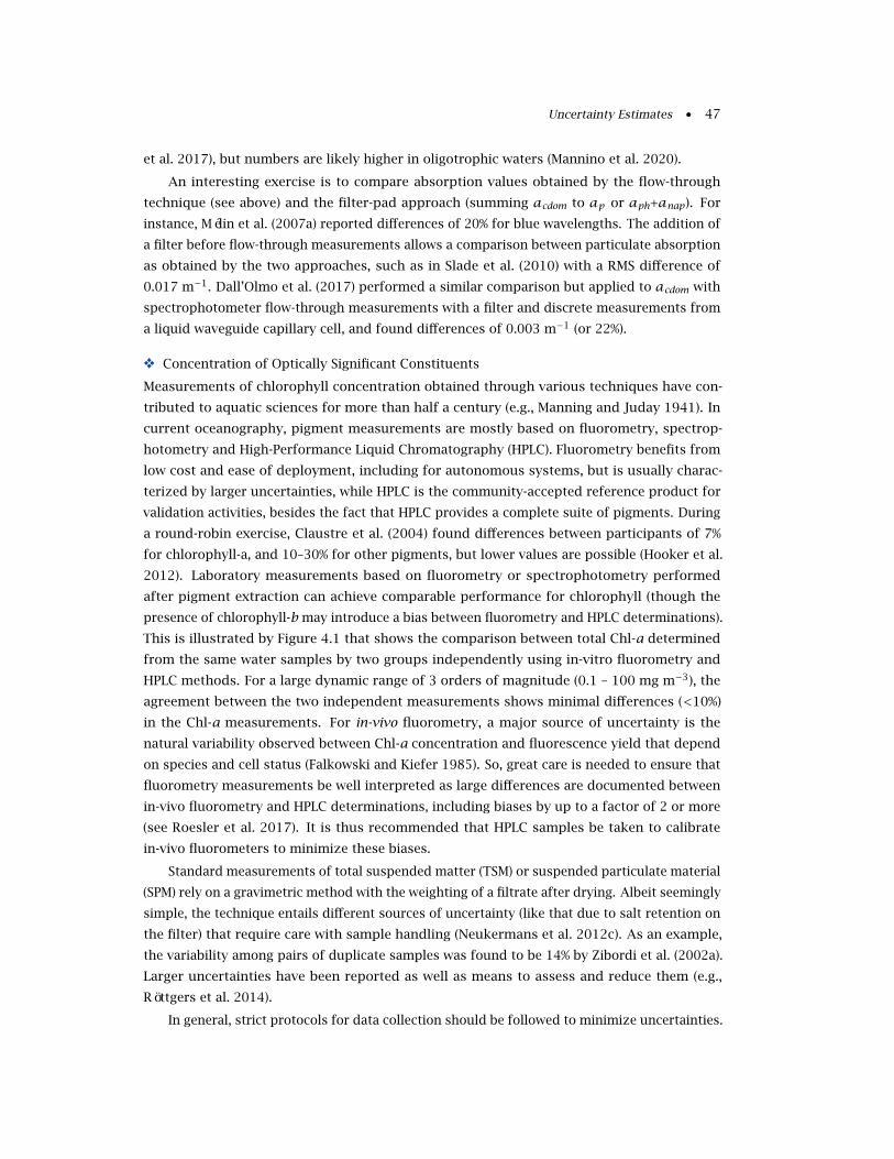
Uncertainty Estimates • 47
et al. 2017), but numbers are likely higher in oligotrophic waters (Mannino et al. 2020).
An interesting exercise is to compare absorption values obtained by the flow-through
technique (see above) and the filter-pad approach (summing acdom to ap or aph+anap). For
instance, Mélin et al. (2007a) reported differences of 20% for blue wavelengths. The addition of
a filter before flow-through measurements allows a comparison between particulate absorption
as obtained by the two approaches, such as in Slade et al. (2010) with a RMS difference of
0.017 m−1. Dall’Olmo et al. (2017) performed a similar comparison but applied to acdom with
spectrophotometer flow-through measurements with a filter and discrete measurements from
a liquid waveguide capillary cell, and found differences of 0.003 m−1 (or 22%).
v Concentration of Optically Significant Constituents
Measurements of chlorophyll concentration obtained through various techniques have con-
tributed to aquatic sciences for more than half a century (e.g., Manning and Juday 1941). In
current oceanography, pigment measurements are mostly based on fluorometry, spectrop-
hotometry and High-Performance Liquid Chromatography (HPLC). Fluorometry benefits from
low cost and ease of deployment, including for autonomous systems, but is usually charac-
terized by larger uncertainties, while HPLC is the community-accepted reference product for
validation activities, besides the fact that HPLC provides a complete suite of pigments. During
a round-robin exercise, Claustre et al. (2004) found differences between participants of 7%
for chlorophyll-a, and 10–30% for other pigments, but lower values are possible (Hooker et al.
2012). Laboratory measurements based on fluorometry or spectrophotometry performed
after pigment extraction can achieve comparable performance for chlorophyll (though the
presence of chlorophyll-b may introduce a bias between fluorometry and HPLC determinations).
This is illustrated by Figure 4.1 that shows the comparison between total Chl-a determined
from the same water samples by two groups independently using in-vitro fluorometry and
HPLC methods. For a large dynamic range of 3 orders of magnitude (0.1 – 100 mg m−3), the
agreement between the two independent measurements shows minimal differences (<10%)
in the Chl-a measurements. For in-vivo fluorometry, a major source of uncertainty is the
natural variability observed between Chl-a concentration and fluorescence yield that depend
on species and cell status (Falkowski and Kiefer 1985). So, great care is needed to ensure that
fluorometry measurements be well interpreted as large differences are documented between
in-vivo fluorometry and HPLC determinations, including biases by up to a factor of 2 or more
(see Roesler et al. 2017). It is thus recommended that HPLC samples be taken to calibrate
in-vivo fluorometers to minimize these biases.
Standard measurements of total suspended matter (TSM) or suspended particulate material
(SPM) rely on a gravimetric method with the weighting of a filtrate after drying. Albeit seemingly
simple, the technique entails different sources of uncertainty (like that due to salt retention on
the filter) that require care with sample handling (Neukermans et al. 2012c). As an example,
the variability among pairs of duplicate samples was found to be 14% by Zibordi et al. (2002a).
Larger uncertainties have been reported as well as means to assess and reduce them (e.g.,
Röttgers et al. 2014).
In general, strict protocols for data collection should be followed to minimize uncertainties.
48 • Uncertainties in Ocean Colour Remote Sensing
Figure 4.1 Chl-a determined from the same water samples by two groups using in-vitrofluorometric and HPLC methods (J. Cannizzaro, University of South Florida, unpublisheddata).
As alluded to in the case of IOPs, uncertainties associated with concentrations of Chl-a or
TSM are not only due to the method of determination but are also affected by various aspects
related to sample collection, handling, transport, storage etc. For instance, tubing and pumping
set-ups (particularly impeller pumps) for underway water collection have been shown to have
a significant impact on phytoplankton determinations (Cetinic et al. 2016) and therefore
comparison of pumped data and non-pumped data should take place (e.g., Figure 3 in Westberry
et al. 2010).
4.1.2 Validation Protocol
Comparison of satellite and in situ values relies on the selection of so-called match-ups,
associating field observations with reasonably coincident satellite data. As explained in Section
3.2.5, if the required data are available, the field observations should be optically weighted
along the vertical to match the response of the sensor. The definition of properties along
the vertical participate to the general issue of definitional differences (see Chapter 2) if the
quantities compared (satellite-derived values versus field observations) are not defined in the
exact same terms. Definitional differences should be avoided or at least clearly identified, and
their potential implications quantified; in other words, comparison should be applied as much
as possible to the same quantities (same pigments, same constituent IOPs, same wavelengths,
etc.).
The construction of the match-up data set is often referred to as a validation protocol.
Typically, S satellite pixels (or grid points in the case of level-3 data) around the location
of the field data are extracted for analysis, usually as a square of S=N×N elements or using
the distance d from the target location (with S proportional to d2). The match-up set can be
characterized by:
i) the time difference between field and satellite data ∆t,
ii) the fraction fv of valid retrievals among the potential satellite elements,
Uncertainty Estimates • 49
iii) the average (or median) value of the satellite data,
iv) the spatial coefficient of variation CVs associated with the satellite data (ratio of standard
deviation and average).
In the case of Nt in situ data collected with a short sampling interval, additional properties can
be defined,
v) the average (or median) value of the field data over an appropriate period,
vi) the temporal coefficient of variation CVt .
The choice of N or S (possibly Nt), the minimum fv required and the maximum allowed for ∆t
and CVs (and possibly CVt) define the validation protocol (Bailey and Wang 2001; Mélin et al.
2003; Bailey and Werdell 2006; Mélin and Franz 2014). Implicit in the protocol is a definition
of what a valid satellite retrieval is, based on the outputs of the flagging system associated
with the atmospheric correction and bio-optical algorithms (Section 5.1). Validation statistics
are relevant for the satellite products distributed to the users only if the flagging schemes
used to discard data in production and validation are identical. For the validation of spectral
quantities like RRS , it is best to run the protocol on the whole spectrum to obtain the same
number of match-up values for all bands and allow the analysis of validation statistics across
the spectrum.
Typical (and recommended) values for these parameters are N from 3 to 5 with fv of
at least 50%, ∆t of less than 1-h up to 4-h, CVs of 15-20% (applied to at least a subset of
wavelengths in case of spectral quantities) (Mélin and Franz 2014). These values should be
adapted according to conditions prevailing at the validation sites (for instance, dynamic coastal
regions versus oligotrophic gyres) to guarantee a comparison as meaningful as possible; on
the other hand, selecting very strict match-up selection criteria might lead to a small number
of match-ups that might no longer offer a suitable statistical basis for a meaningful diagnostic
(e.g., Figure 2 in Haëntjens et al. 2017). In general, it is expected that validation statistics
might change with the adopted selection criteria (Mélin et al. 2007a; Barnes et al. 2019) and the
comparison between validation statistics obtained in various locations must be conducted with
due consideration. The differing characteristics of level-2 or level-3 data also imply different
match-up selection criteria, which in turn may lead to different numbers of match-ups and
validation results (Scott and Werdell 2019); as a corollary, validation statistics obtained with
level-2 data are applicable to higher processing levels only with a degree of caution.
As anticipated above, the differences between field and satellite data are partly explained
by mismatches in time and spatial scales (comparison of pixel-size or grid points with point
measurements or water samples collected at sea), but appropriate values of ∆t and CV might
limit this issue of representativeness. This being said, studies addressing decorrelation
time and space scales of optical properties in the ocean and atmosphere should help better
characterize comparisons between field and satellite data. A more thorough analysis, taking
advantage of measurements collected at fine spatial scales (e.g., Yuan et al. 2005; Brewin et al.
2016) and with a vertical resolution, would certainly be useful to better assess validation
statistics in relation to representativeness. In that regard, measurements collected at scales
of the order of tens of meters and/or minutes could be beneficial if global missions (with
resolution of hundreds of meters) are considered. From the atmospheric point of view,
50 • Uncertainties in Ocean Colour Remote Sensing
some measurements have shown that time lags of 1- to 3-h resulted in small decrease in the
autocorrelation of the aerosol optical thickness τa (Anderson et al. 2003). But still, coefficients
of variation of 5–10% within a couple of hours can be noticed for τa at coastal sites such as
the AAOT (Adriatic Sea) (Mélin et al. 2007b). At the same location, above-water measurements
of RRS indicate variations of 4% in the blue-to-green spectral interval and 9% in the red (Mélin
and Zibordi 2007); it may be noticed that these values are actually similar to the uncertainties
associated with these measurements (Gergely and Zibordi 2014). In regions under strong
influence of tides, temporal variations in optical properties can be larger (Liu and Wang
2016; Zhang et al. 2018). Spatially, some experiments suggest typical length scales of 10s
to 100s meters in coastal regions for turbidity and fluorescence (Blackwell et al. 2008). The
appearance of high-resolution sensors appropriate for OC measurements (even though still
characterized by low signal-to-noise ratios) has the potential to help illustrating the issue of
representativeness. Using imagery over the AERONET-OC sites from OLI on-board Landsat-8,
the results of Pahlevan et al. (2016) suggest differences for RRS of ∼4% (8% in the red) between
scales associated with OLI (30-m resolution) and MODIS or VIIRS-size pixels but in some cases
these differences could reach 18%. These authors also conclude that in coastal waters, selecting
only one pixel (closest to the location of interest) for the comparison with field data is limiting
differences (while it might reinforce issues such as noise or striping). Overall these numbers,
comparable to the uncertainty objectives for RRS (see Section 6.1), are therefore significant and
highlight the importance of well-defined validation protocols together with a good knowledge
of conditions at the validation sites.
Another issue regards the validation of spectral quantities, be it remote sensing reflectance,
inherent optical properties or aerosol optical thickness: the spectral characteristics of field
and satellite data usually differ. This point is particularly relevant as even small differences in
wavelength or spectral response can lead to significant differences in water-leaving radiance
or remote sensing reflectance (Mélin and Sclep 2015; Zibordi et al. 2017). For data sets with
fairly constant spectral shapes, they easily lead to biases in validation statistics. To correct for
these spectral inconsistencies, spectral relationships have often been employed in validation
analyses of LWN and RRS (e.g., Zibordi et al. 2006; Antoine et al. 2008) or τa (Mélin et al. 2007b;
Mélin 2010); in recent years dedicated approaches were proposed to address this issue of
band-shifting (Mélin and Sclep 2015; Pahlevan et al. 2017; Li et al. 2018; Hieronymi 2019). The
uncertainties associated with these procedures should be duly accounted for in an overall
budget as they can be significant, amounting to a few percent when spectral differences exceed
5 nm and/or in optically complex waters (e.g., Mélin and Sclep 2015; Li et al. 2018).
A last point to consider is associated with geometry. If the time differs between satellite
and field acquisitions, the conditions of illumination are different, while the geometry of
observation is usually different. These differences are corrected by working with normalized
quantities (LWN or RRS , Morel and Gentili 1996) for both satellite and field data, but corrections
for the bidirectional effects are affected by uncertainties as discussed in Section 3.2.7. A way
to minimize the impact of bidirectional effects in validation studies is to adopt the same model
for both satellite and in situ data; in practice, this is not necessarily appropriate as bidirectional
corrections can be tuned for in situ data in cases where additional information is available
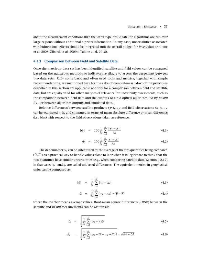
Uncertainty Estimates • 51
about the measurement conditions (like the water type) while satellite algorithms are run over
large regions without additional a priori information. In any case, uncertainties associated
with bidirectional effects should be integrated into the overall budget for in situ data (Antoine
et al. 2008; Zibordi et al. 2009b; Talone et al. 2018).
4.1.3 Comparison between Field and Satellite Data
Once the match-up data set has been identified, satellite and field values can be compared
based on the numerous methods or indicators available to assess the agreement between
two data sets. Only some basic and often used tools and metrics, together with simple
recommendations, are mentioned here for the sake of completeness. Most of the principles
described in this section are applicable not only for a comparison between field and satellite
data, but are equally valid for other analyses of relevance for uncertainty assessments, such as
the comparison between field data and the outputs of a bio-optical algorithm fed by in situ
RRS , or between algorithm outputs and simulated data.
Relative differences between satellite products (yi)i=1,N and field observations (xi)i=1,N
can be expressed in %, and computed in terms of mean absolute difference or mean difference
(i.e., bias) with respect to the field observations taken as reference:
|ψ| = 1001N
N∑i=1
|yi − xi|xi
(4.1)
ψ = 1001N
N∑i=1
yi − xixi
(4.2)
The denominator xi can be substituted by the average of the two quantities being compared
(xi+yi2 ) as a practical way to handle values close to 0 or when it is legitimate to think that the
two quantities have similar uncertainties (e.g., when comparing satellite data, Section 4.2.12).
In that case, |ψ| and ψ are called unbiased differences. The equivalent metrics in geophysical
units can be computed as:
|δ| = 1N
N∑i=1
|yi − xi| (4.3)
δ = 1N
N∑i=1
(yi − xi) = y − x (4.4)
where the overbar means average values. Root-mean-square differences (RMSD) between the
satellite and in situ measurements can be written as:
∆ =
√√√√√ 1N
N∑i=1
(yi − xi)2 (4.5)
∆c =
√√√√√ 1N
N∑i=1
(yi −y − xi + x)2 =√∆2 − δ2 (4.6)
52 • Uncertainties in Ocean Colour Remote Sensing
The total root-mean-square difference ∆ can be partitioned in a part due to the bias δ and
the unbiased (or centered) root-mean-square difference ∆c quantifying non-systematic effects.
RMS differences can also be expressed in relative terms.
In the above equations, the summation operator has been used (which means that quan-
tities are averages), but other operators can be used like the median, or some inter-quantile
statistics. Filtering through the match-up data set to treat outliers can also be appropriate in
some cases. Related to ψ is the average ratio:
ρ = 1N
N∑i=1
yixi
(4.7)
Other metrics can be included like the coefficient of determination r 2, defined as (Pearson
coefficient):
r 2 =
(∑Ni=1(xi − x)(yi −y)
)2
∑Ni=1(xi − x)2
∑Ni=1(yi −y)2
(4.8)
or slope and intercept of linear regression. Model I regression (with its use of ordinary least-
squares criterion) assumes that one variable is error-free, which is not the case when in situ
data are the data of reference. Uncertainties in in situ data can be taken into account by using
a Method II regression, simplifying to a major-axis regression if uncertainties of the data being
compared are assumed similar (Legendre and Legendre 1998). If uncertainty estimates are
available for individual data points, a weighted regression should be used so that points with
large uncertainties weigh less than those with low uncertainties.
For spectral quantities like RRS input to bio-optical algorithms, quantifying how well the
spectral shape is respected by the satellite products is also worthy information, that can be
quantified by a χ2 distribution measuring the goodness of fit between in situ and satellite RRSnormalized at one wavelength of reference.
A logarithmic transformation (typically for Chl-a or IOPs) applied prior to statistical
calculations might be appropriate according to the range and distributions of values. However,
if the data are transformed in logarithmic space before applying the statistical measures above,
relative differences (such as Equations 4.1 and 4.2) are no longer appropriate: metrics written
as simple differences (e.g., Equations 4.3 to 4.5) are already expressed in relative terms (the
difference of logarithms being equal to the logarithm of the ratio of the two arguments). For
radiometric products, experience suggests the importance of documenting both a measure of
uncertainty in radiometric units (sr−1 for RRS ) and a measure of relative uncertainty (Zibordi
et al. 2009a; Mélin et al. 2011b). Indeed, relative differences tend to be large for low signals
(up to tens of percent if the in situ value is near zero, see also Section 4.3.1). In that case, the
difference in radiometric units might be more meaningful; as said above, unbiased relative
differences might also be preferred but this suggests comparable uncertainties for both
quantities being compared. If appropriate, the sensitivity of the validation results to a specific
datum or to subsets of the match-up ensemble can be tested by bootstrapping techniques
(Brewin et al. 2015).
Uncertainty Estimates • 53
Most of the statistics introduced above are pair-wise quantities, typically comparing
a pixel value with a field observation value. Besides being useful to address the issue of
representativeness as discussed in the previous section, the use of measurement systems
with fast temporal acquisition and/or high spatial resolution (for instance with autonomous
devices or flow-through systems, Brewin et al. 2016) might require a pre-processing of the field
observations before the comparison with satellite data can be done and interpreted. Ideally,
time and/or space binning of field data should be conducted taking into account the resolution
of the space sensor as well as time and space scales characteristic of the observed fields.
The selection of one quantity to the detriment of others to assess a product or to rank
algorithms has been the subject of debates (e.g., Chai and Draxler 2014, about RMS and mean
absolute differences); ultimately each quantity has pros and cons (sensitivity to outliers, inter-
pretation when data distributions are not normal etc.) and should be interpreted with caution
in the context of well-defined hypotheses (e.g., normality of the uncertainty distribution). It
seems also clear that only one of these quantities can hardly summarize a complete view of
the distributions between the considered data sets. When documenting a match-up exercise,
besides the number of match-ups, reporting estimates of the scatter and systematic difference
(bias) between the two distributions seems a minimum (Mélin and Franz 2014). Algorithm
performance ranking based on these statistical indicators is certainly not straightforward, as
each can favor a different algorithm. The task is even harder in the case of spectral quantities
as one algorithm can be optimal for a wavelength and not for others. Methods to perform that
ranking have been proposed (Brewin et al. 2015; Mueller et al. 2015a) but ultimately a part of
subjectivity is likely to remain in relation to user applications and requirements.
Various graphical methods have been devised to help in representing validation results.
Obviously, results associated with spectral quantities can be plotted as a function of wavelength.
Target diagrams represent along two axes the centered-RMSD ∆c and the bias δ (and therefore
the RMSD ∆, Equation 4.6, Jolliff et al. 2009; Mélin and Franz 2014). Taylor plots (Taylor 2001)
are based on triangular relationships to contemporaneously illustrate the correlation coefficient
r , the centered-RMSD ∆c and the respective standard deviations of data sets. In the field of
ocean colour, they have been used to compare the performance of bio-optical algorithms (Mélin
et al. 2007a; Werdell et al. 2013). An evolution is proposed by Correa and Lindstrom (2013)
in the form of Mutual Information Diagram that has already been used to compare satellite
products (Belo Couto et al. 2016). Star, or radar, plots also provide an effective graphical
approach for evaluating the behavior of algorithms across multiple uncertainty metrics. Here,
the plot centre represents values indicating poor algorithm performance such that spokes
(rays) for the best performing approach reaches farthest from the center (e.g., Seegers et al.
2018).
Some OC products do not lend themselves easily to the application of the difference
indicators listed above. This is the case for discrete quantities such as membership to classes
(optical water types or multi-variable classes), phytoplankton groups or types, size classes,
cell counts intervals, diversity indices, detection of specific blooms, phenology metrics, etc.
In these cases, other methods may need to be used to assess the performance of algorithms
or the uncertainties of satellite products, for instance relying on contingency matrices or
54 • Uncertainties in Ocean Colour Remote Sensing
classification indices (Congalton 1991; Liu et al. 2007). Such techniques have been used to
assess phytoplankton size classes (Brewin et al. 2011), the occurrences of harmful algal blooms
(Carvalho et al. 2011; Lunetta et al. 2015), the presence of specific algae like Sargassum (Wang
and Hu 2017) or Chl-a trends (Mélin et al. 2017).
Regardless of the quantities used or their graphical display, an important point is to be
kept in mind when interpreting validation results in a larger context: they are really applicable
to a given satellite product only if the frequency distributions of the field and satellite data are
similar.
4.2 Methods for Identifying Out-of-Scope Conditions and Estimating
Uncertainties of Ocean Colour Products
The first sub-section below presents approaches to identification of out-of-scope conditions,
or conversely, the definition of the domain of applicability of an algorithm. This step defines
the framework in which an algorithm can be applied with some degree of confidence and
participates to the process of quality control. Then various approaches that have been applied
in the field of OC remote sensing to provide uncertainty estimates are summarized and
illustrated. Some are fairly specific to the field (e.g., the so-called clear water approach, or
the use of optical water types), while others have been already employed for other types of
geophysical data (e.g., co-location experiments). Some are based on the principles of uncertainty
propagation. Among the forward uncertainty propagation approaches here illustrated are
expansion-based approaches (e.g., relying on Taylor series) and simulation-based methods (e.g.,
Monte-Carlo simulations). The use of a Bayesian framework is also documented as example of
inverse uncertainty quantification. It is stressed that other categories of approaches (including
some advanced techniques) exist for uncertainty quantification (e.g., Padulo et al. 2007; Lee
and Chen 2009) but have not yet received much attention from the OC community.
4.2.1 Identification of Out-of-Scope Conditions
Some conditions in the field of view of a sensor are not conducive to a proper data treatment as
envisioned by algorithm developers. In an operational framework, space agencies have included
so-called flags along the processing chain (Figure 3.3), that is to say, warning diagnostics urging
caution in the use of the data, or go/no-go breaking points where the processing might not
proceed, leading to masked pixels (Robinson et al. 2003; OLCI 2010b,c). The overall objective
is to assure a certain level of quality to the derived products. Some flags are associated
with the functioning of the sensors, in relation to a saturated signal or a navigation failure.
Another tier of flags typically prevents, or at least signals, the operation of the atmospheric
correction algorithm for conditions presumably not well handled by the algorithm, pertaining
to geometry (high zenith angles for Sun or viewing angle) or to atmosphere and water surface
conditions (presence of land, clouds, cloud shadows, thick aerosol plumes, sea ice, Sun glint).
The operation of the atmospheric correction itself might generate its own flags indicating
a non-optimal functioning (lack of convergence, negative RRS , aerosol characteristics out of
Uncertainty Estimates • 55
algorithm bounds etc.). An additional tier of flags similarly informs the use of any bio-optical
algorithm retrieving water properties. Most of these flags are specific to a certain algorithm
and/or to a certain degree of requirements. In general, releasing the thresholds defining the
flagging tests means an increase in spatial coverage but a degradation of product quality, and
space agencies have tended to be rather conservative with regards to global application. One
well-known consequence is that, in the case of standard products, pixels may be masked out
in coastal regions with cloud-free conditions and fairly bright water surface in association with
high sediment concentration (Okana et al. 2003) or intense blooms (Banks and Mélin 2015).
The set of flags applied in the processing defines out-of-scope conditions or, equivalently, the
conditions for which a processing is conducted and for which uncertainty estimates are needed.
This means that a change in the flagging system might entail a revision of the uncertainty
budget. Other remote sensing communities have defined quality flags, where higher values
mean an increased confidence in the data and a consequent extension of the applications
deemed appropriate for that level of confidence (Kilpatrick et al. 2001).
Downstream from the application of flags, out-of-scope conditions may be further detected
considering algorithm inputs and outputs. Purely empirical algorithms are developed from data
bases of field or simulated data and even semi-analytical algorithms may rely on parameters
representative of a given dataset. This has often been the case for regional applications, but
obviously regional empirical algorithms may not be applicable in other regions (e.g., D’Alimonte
et al. 2012). More generally, the application of an algorithm for observation conditions that are
not representative of its training data set is unwarranted. Some easy checks can be performed
in the case of simple algorithms: for instance the direct relationship between a reflectance
band-ratio and Chl-a should not be applied out of the bounds of the training data.
For more complex algorithms such as those based on neural networks (NN), it is possible
to devise an approach using an auto-associative NN to estimate if an input is represented
within the training data set. This has been implemented for a NN-based atmospheric correction
applied to MERIS (4th reprocessing) and OLCI for Case-2 water products (OLCI 2010a; Doerffer
2010, 2015). In practice, the top-of-atmosphere reflectance spectrum, ρTOA (after correction
for gaseous absorption) is fed into an auto-associative NN, which produces ρ′TOA after ρTOA
has passed a bottleneck layer in the NN. The number of neurons of this bottleneck has to be as
small as possible to just reproduce the simulated training data with only a tiny error. In the
case that a measured ρTOA spectrum is out-of-scope of the training data, the deviation between
the input and output spectrum is increased and may exceed a given threshold, triggering the
out-of-scope flag. Out-of-scope water-leaving reflectances ρw resulting from the atmospheric
correction are identified with a different method. The IOPs, derived from ρw using an in-water
NN, are fed into another forward NN to reproduce water-leaving reflectance, ρ′w . ρw and ρ′ware then compared in the same way as ρTOA. If the deviation exceeds a given threshold, a flag
is triggered. Typical out-of-scope conditions for the standard Case-2 water NNs can be found
for example in the estuary of the Rio de la Plata, which contains extremely high concentrations
of particles.
Out-of-scope conditions can also be detected with respect to a set of optical water types
(also called classes). Classification of natural waters, recognizing that different types of water
56 • Uncertainties in Ocean Colour Remote Sensing
can be distinguished on the basis of their optical signature, started early (Arnone et al. 2004),
and includes the types listed by Jerlov (1976) or the distinction between Case-1 and Case-2
waters (Morel and Prieur 1977). Case-1 waters, typically found in the open ocean, are those
where phytoplankton, its derivation products and covarying particles (e.g., bacteria) dominate
the optical properties of the water, and a simplified framework expresses all optical properties
as a function of the concentration of chlorophyll-a (Morel and Maritorena 2001). Conversely,
algorithms developed for Case-1 waters have been considered as unsuitable for application
in coastal waters, or at least subject to high uncertainties, and tests have been developed to
operate the distinction Case-1/Case-2 (e.g., Loisel and Morel 1998; Lee and Hu 2006). Along the
same line, some phenomena in the ocean have been related to specific optical properties and
can be detected accordingly, including blooms of coccolithophores (Brown and Yoder 1994;
Shutler et al. 2010; Moore et al. 2012) or Trichodesmium (Subramaniam et al. 2002; Hu et al.
2010) and patches of floating Sargassum (Gower et al. 2006; Qi et al. 2017a). As a corollary,
these conditions are usually considered out of the scope of application of standard algorithms.
More general classification approaches have been proposed to identify distinct water types
or classes or to operate quality control using training data sets of remote sensing reflectance
obtained from field observations or satellite data (Moore et al. 2001; D’Alimonte et al. 2003;
Martin-Traykovski and Sosik 2003; D’Alimonte and Zibordi 2006; Mélin and Vantrepotte
2015; Wei et al. 2016). Utilizing a class-based approach relies on the assumption that the
optical characteristics and related algorithms associated with a given class are valid for any
RRS spectrum having a high membership in relation to that class. To the contrary, a low
membership means that class-specific properties are unlikely to be verified in the condition
associated with RRS . If a specific algorithm is available for each class, it is possible to combine
the outputs of the class-specific algorithms into a seamless product distribution (Moore et al.
2001, 2014; D’Alimonte et al. 2003; Mélin et al. 2011a; Vantrepotte et al. 2012). In that
operation, the contribution of each algorithm is weighted by the associated class membership
(see also Section 4.2.5). By the same token, this exercise is equivalent to a novelty detection: if
a class membership is low, the observed condition (expressed by RRS ) is novel with respect
to the information content of the class and the class-specific algorithm should be considered
as outside its range of applicability (D’Alimonte et al. 2003, 2014). An important point to
remember in that framework is the dependence on the training data set; if an input spectrum
RRS is associated with low class memberships or considered as an anomaly by a quality control
system, it might not necessarily mean that RRS is an invalid spectrum: it might just be outside
the conditions covered by the training data.
Somewhat extending the definition of out-of-scope conditions, it can be noticed that
post-processing checks can be carried out to detect anomalous conditions, including out-of-
bound output values, unrealistic spatial features (like sharp gradients), values far from local
climatology, or outliers with respect to current conditions. In the latter case, spatial coherence
techniques have been proposed to detect outliers within a spatial distribution (for instance
using empirical orthogonal functions, Alvera-Azcárate et al. 2012).
Uncertainty Estimates • 57
4.2.2 Assessment from Algorithm Construction
There are necessarily subjective choices made about the structure of an algorithm, and the
very process of building an algorithm, if well thought out, should already provide information
on the expected sources and types of uncertainties as well as its domain of applicability. This
step can rely on prior statistical analysis or expert judgment, leading to distinction of Types A
and B uncertainty types (see Chapter 2). As far as possible, uncertainties on specific algorithm
parameters should be defined in that process.
The construction of some algorithms relies on regression analyses, for instance in the
case of a purely empirical ones (using field or simulated data, with simple functional forms or
more complex ones such as neural networks). Statistics characterizing the fit between training
data and model output (RMS of the residuals, correlation coefficient etc.) should be reported
as completely as possible. To some extent the RMS of the residuals might be considered
as minimum values of the uncertainty associated with the algorithm. It should however be
remembered that regression statistics are associated with the overall fit while the quality of
the fit might vary across the range of considered values, so that the related uncertainties
might vary as well. On the other hand, when using field observations for the regression, it is
possible that their own uncertainties degrade the regression statistics. Independently of how
far these interpretations can be carried, they are in any case valid only when the algorithm
is applied to conditions well represented within the training data. When building the OC4v4
maximum-band-ratio algorithm for Chl-a, O’Reilly et al. (2000) reported a RMS value for the
residuals equal to 0.22 on the (log-transformed) training data. As a comparison, Gregg and
Casey (2004) obtained a RMS difference between SeaWiFS-derived and in situ Chl-a of 0.31
using globally distributed match-ups, an increase in value that is easily attributable to the
treatment of satellite data.
The confidence in the statistics obtained through the regression on a training data set
can be enhanced by setting aside part of the data for validation purposes. This is however
limited to cases with large data sets and the impact of the selected division might not be well
controlled. Of more general application is a cross-validation process. The actual technique can
be carried out in various ways (e.g., Arlot and Celisse 2010) but relies on repeated divisions
of the available data set into a training set (used for the construction of the algorithm) and a
validation set (used to evaluate the performance of the algorithm). This operation is repeated
various times with subjective or random selections of the divisions, and validation statistics
(together with regression statistics) are available for each realization. Cross-validation entails
more calculations but lessens the risks of over-fitting and the impact of outliers, and ultimately
provides a more faithful view of the algorithm behavior. Cross-validation has already been
used in the ocean colour community, for instance to construct empirical algorithms for Chl-a
retrieval (D’Alimonte and Zibordi 2003), but a more general application would certainly be
good practice.
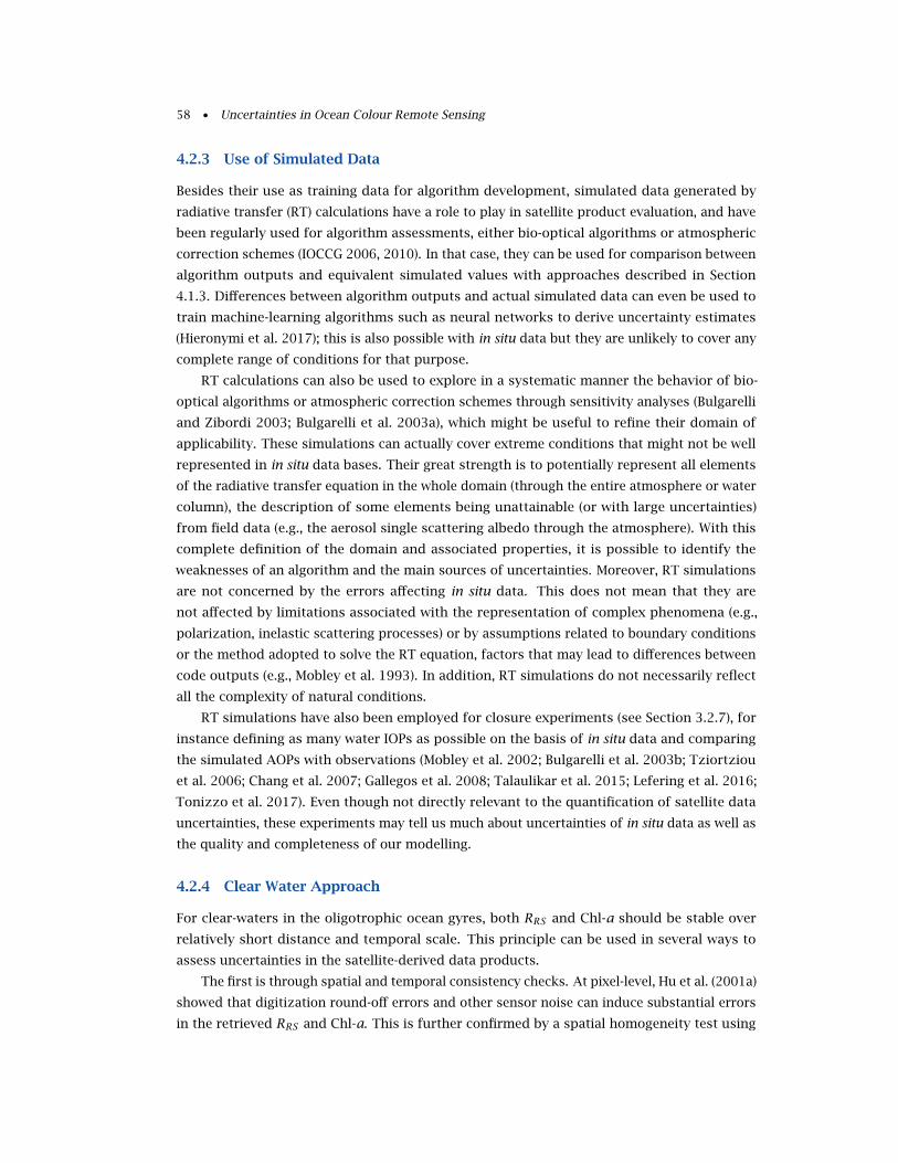
58 • Uncertainties in Ocean Colour Remote Sensing
4.2.3 Use of Simulated Data
Besides their use as training data for algorithm development, simulated data generated by
radiative transfer (RT) calculations have a role to play in satellite product evaluation, and have
been regularly used for algorithm assessments, either bio-optical algorithms or atmospheric
correction schemes (IOCCG 2006, 2010). In that case, they can be used for comparison between
algorithm outputs and equivalent simulated values with approaches described in Section
4.1.3. Differences between algorithm outputs and actual simulated data can even be used to
train machine-learning algorithms such as neural networks to derive uncertainty estimates
(Hieronymi et al. 2017); this is also possible with in situ data but they are unlikely to cover any
complete range of conditions for that purpose.
RT calculations can also be used to explore in a systematic manner the behavior of bio-
optical algorithms or atmospheric correction schemes through sensitivity analyses (Bulgarelli
and Zibordi 2003; Bulgarelli et al. 2003a), which might be useful to refine their domain of
applicability. These simulations can actually cover extreme conditions that might not be well
represented in in situ data bases. Their great strength is to potentially represent all elements
of the radiative transfer equation in the whole domain (through the entire atmosphere or water
column), the description of some elements being unattainable (or with large uncertainties)
from field data (e.g., the aerosol single scattering albedo through the atmosphere). With this
complete definition of the domain and associated properties, it is possible to identify the
weaknesses of an algorithm and the main sources of uncertainties. Moreover, RT simulations
are not concerned by the errors affecting in situ data. This does not mean that they are
not affected by limitations associated with the representation of complex phenomena (e.g.,
polarization, inelastic scattering processes) or by assumptions related to boundary conditions
or the method adopted to solve the RT equation, factors that may lead to differences between
code outputs (e.g., Mobley et al. 1993). In addition, RT simulations do not necessarily reflect
all the complexity of natural conditions.
RT simulations have also been employed for closure experiments (see Section 3.2.7), for
instance defining as many water IOPs as possible on the basis of in situ data and comparing
the simulated AOPs with observations (Mobley et al. 2002; Bulgarelli et al. 2003b; Tziortziou
et al. 2006; Chang et al. 2007; Gallegos et al. 2008; Talaulikar et al. 2015; Lefering et al. 2016;
Tonizzo et al. 2017). Even though not directly relevant to the quantification of satellite data
uncertainties, these experiments may tell us much about uncertainties of in situ data as well as
the quality and completeness of our modelling.
4.2.4 Clear Water Approach
For clear-waters in the oligotrophic ocean gyres, both RRS and Chl-a should be stable over
relatively short distance and temporal scale. This principle can be used in several ways to
assess uncertainties in the satellite-derived data products.
The first is through spatial and temporal consistency checks. At pixel-level, Hu et al. (2001a)
showed that digitization round-off errors and other sensor noise can induce substantial errors
in the retrieved RRS and Chl-a. This is further confirmed by a spatial homogeneity test using
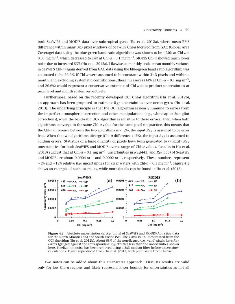
Uncertainty Estimates • 59
both SeaWiFS and MODIS data over subtropical gyres (Hu et al. 2012a), where mean RMS
difference within many 3x3 pixel windows of SeaWiFS Chl-a (derived from GAC (Global Area
Coverage) data using the blue-green band ratio algorithm) was shown to be ∼30% at Chl-a =
0.03 mg m−3, which decreased to 14% at Chl-a = 0.1 mg m−3. MODIS Chl-a showed much lower
noise due to increased SNR (Hu et al. 2012a). Likewise, at monthly scale, mean monthly variance
in SeaWiFS Chl-a (again derived from GAC data using the blue-green band ratio algorithm) was
estimated to be 26.6%. If Chl-a were assumed to be constant within 3×3 pixels and within a
month, and excluding systematic contributions, these measures (14% at Chl-a = 0.1 mg m−3,
and 26.6%) would represent a conservative estimate of Chl-a data product uncertainties at
pixel level and month scales, respectively.
Furthermore, based on the recently developed OCI Chl-a algorithm (Hu et al. 2012b),
an approach has been proposed to estimate RRS uncertainties over ocean gyres (Hu et al.
2013). The underlying principle is that the OCI algorithm is nearly immune to errors from
the imperfect atmospheric correction and other manipulations (e.g., whitecap or Sun glint
corrections), while the band-ratio OCx algorithm is sensitive to these errors. Then, when both
algorithms converge to the same Chl-a value for the same pixel (in practice, this means that
the Chl-a difference between the two algorithms is < 5%), the input RRS is assumed to be error
free. When the two algorithms diverge (Chl-a difference > 5%), the input RRS is assumed to
contain errors. Statistics of a large quantity of pixels have been generated to quantify RRSuncertainties for both SeaWiFS and MODIS over a range of Chl-a values. Results in Hu et al.
(2013) suggest that at Chl-a = 0.1 mg m−3, uncertainties in RRS (443) and RRS (555) of SeaWiFS
and MODIS are about 0.0004 sr−1 and 0.0002 sr−1, respectively. These numbers represent
∼5% and ∼12% relative RRS uncertainties for clear waters with Chl-a = 0.1 mg m−3. Figure 4.2
shows an example of such estimates, while more details can be found in Hu et al. (2013).
Figure 4.2 Absolute uncertainties (in RRS units) of SeaWiFS and MODIS/Aqua RRS datafor the North Atlantic (NA) and South Pacific (SP). The x-axis is Chl-a estimated from theOCI algorithm (Hu et al. 2012b). About 68% of the non-flagged (i.e., valid) pixels have RRSerrors (gauged against the corresponding RRS “truth”) less than the uncertainties shownhere. Pixelization noise has been removed using a 3x3 median filter before uncertaintycalculations. Figure reproduced from Hu et al. (2013) with permission from Elsevier.
Two notes can be added about this clear-water approach. First, its results are valid
only for low Chl-a regions and likely represent lower bounds for uncertainties as not all
60 • Uncertainties in Ocean Colour Remote Sensing
components (such as systematic effects) are taken into account. Then, results suggest that
the RRS errors from individual pixels (as gauged by the RRS “truth”) are spectrally related
rather than spectrally independent. This has significant implications for algorithm design, as
for example the band-subtraction OCI algorithm can suppress nearly all these errors in the
retrieved Chl-a (Hu et al. 2012b). For example, a 100% RRS error at 555 nm would induce only
5% Chl-a error in such an algorithm. Moreover, such spectral relationships can be put to use
into bio-optical algorithms to improve the calculation of IOPs (Chen et al. 2016).
4.2.5 Approach based on Optical Water Types
As introduced in Section 4.2.1, classification techniques, typically applied on RRS spectra, can
be used to detect out-of-scope conditions, or map the range of applicability of class-specific
algorithms, as well as combine their outputs (Moore et al. 2001, 2014; D’Alimonte et al. 2003;
Mélin et al. 2011a). Several investigations have analysed validation results in the framework
of optical water types (OWTs) or classes (Moore et al. 2009, 2015; Goyens et al. 2013; Mélin
and Franz 2014). If enough data are available to define uncertainty values for each class,
this information can be extended through the classification of any input RRS . Here again,
the assumption is that results obtained for a class are valid for any observation with a high
membership with respect to that class. Moore et al. (2009) followed this path to map the
uncertainties associated with the MODIS Chl-a global distributions, using field observations
primarily from the NOMAD data base to construct the set of OWTs, while the MODIS validation
data set (Bailey and Werdell 2006) was used to define validation statistics for each water type.
A similar approach has been adopted by the Ocean Colour Climate Change Initiative (OC-CCI)
of the European Space Agency (ESA) (Jackson et al. 2017). It has also been used for more
advanced products such as phytoplankton groups (Brewin et al. 2017b).
Mathematically, the approach can be summarized as follows. The approach first requires
the definition of uncertainty estimates for each class k of a set of K water types. In the case
of OWTs, these are defined on the basis of RRS data, but the definition of the classes can rely
on other quantities. If these uncertainty estimates are based on validation statistics obtained
from the comparison of match-up satellite products (yi)i=1,N and field observations (xi)i=1,N ,
the same statistics can be computed for each class k. For the examples of the RMS difference
and bias, they are written as weighted averages of the related statistics for each match-up:
∆k =
√√√√∑Ni=1wk,i(yi − xi)2∑Ni=1wk,i
(4.9)
δk =∑Ni=1wk,i(yi − xi)∑N
i=1wk,i(4.10)
where the weight wk,i is the class membership of the matchup i in class k, quantifying how
much match-up i contributes to the definition of the uncertainty estimates associated with
class k. Similar equations can be written for other metrics. It is noted that this approach can be
applied to a variable (represented by x and y) that is different from the classifying quantities:
for instance, class-specific uncertainties can be computed for Chl-a for OWTs defined by RRS
Uncertainty Estimates • 61
data. As far as the latter are concerned, they can come from field observations or from satellite
data (Moore et al. 2012; Mélin and Vantrepotte 2015; Jackson et al. 2017). Using satellite data
to construct the set of classes have some advantages: they are ultimately the data that will be
used for classification at large scales and they potentially allow a more complete sampling of
the full natural variability than a set of field observations. Figure 4.3 shows the ∆’s obtained
for log-transformed Chl-a and for the RRS -based classes used by the OC-CCI project for global
applications (Jackson et al. 2017).
Figure 4.3 RMS differences ∆ obtained from Equation 4.9 in association with the setof classes defined by the OC-CCI project for global applications (Jackson et al. 2017).Increasing class numbers approximately parallels a shift from open ocean to coastalwaters. Figure reproduced from Jackson et al. (2017) with permission from Elsevier.
Once validation statistics are available for each class, similar statistics can be computed
for any input data. Any validation metric for that input can be expressed as a weighted average
of the statistics obtained for the set of classes, where the weights are the class memberships
(wk)k=1,K found for that input. Again for the examples of RMS difference and bias, this gives:
∆ =
√√√√∑Kk=1wk∆2k∑K
k=1wk(4.11)
δ =∑Kk=1wkδk∑Kk=1wk
(4.12)
where again ∆k and δk are values defined for class k.
The strength of this approach is that uncertainty estimates are directly traceable to in situ
data and thus potentially to standards. On the other hand in the current implementation, it
does not take into consideration that in situ data have their own uncertainties, affecting the
construction of the classes (unless satellite data are used for that purpose) and validations
statistics. Moreover, the scheme depends on match-up data that might not be available in large
numbers for all water types and/or all considered variables.
4.2.6 Outputs of Non-Linear Inversion Methods
Non-linear least squares inversion bio-optical algorithms commonly adopt gradient-based
methods to generate uncertainties in their output products (typically, spectral IOPs, namely
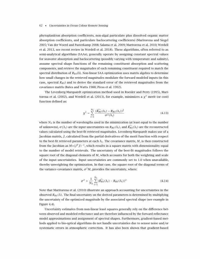
62 • Uncertainties in Ocean Colour Remote Sensing
phytoplankton absorption coefficients, non-algal particulate plus dissolved organic matter
absorption coefficients, and particulate backscattering coefficients) (Maritorena and Siegel
2005; Van der Woerd and Pasterkamp 2008; Salama et al. 2009; Maritorena et al. 2010; Werdell
et al. 2013, see recent review in Werdell et al. 2018). These algorithms, often referred to as
semi-analytical algorithms (SAAs), generally operate by assigning constant spectral values
for seawater absorption and backscattering (possibly varying with temperature and salinity),
assume spectral shape functions of the remaining constituent absorption and scattering
components, and retrieve the magnitudes of each remaining constituent required to match the
spectral distribution of RRS (λ). Non-linear SAA optimization uses matrix algebra to determine
how small changes in the retrieved magnitudes modulate the forward modeled inputs (in this
case, spectral RRS ) and to derive the standard error of the retrieved magnitudes from the
covariance matrix (Bates and Watts 1988; Press et al. 1992).
The Levenberg-Marquardt optimization method used in Roesler and Perry (1995), Mari-
torena et al. (2002), and Werdell et al. (2013), for example, minimizes a χ2 merit (or cost)
function defined as:
χ2 =Nλ∑i=1
(RRS(λi)− RRS(λi))2σ 2(λi)
(4.13)
where Nλ is the number of wavelengths used in the minimization (at least equal to the number
of unknowns), σ(λi) are the input uncertainties on RRS(λi), and RRS(λi) are the reconstructed
values calculated using the best-fit retrieved magnitudes. Levenberg-Marquardt makes use of a
Jacobian matrix, J, calculated from the partial derivatives of the merit function with respect
to the best-fit retrieved parameters at each λi. The covariance matrix, M , is then constructed
from the Jacobian as M=(JTJ)−1, which results in a square matrix with dimensionality equal
to the number of model retrievals. The uncertainty of the best-fit magnitudes follows the
square root of the diagonal elements of M , which accounts for both the weighting and scale
of the input uncertainties. Input uncertainties are commonly set to 1.0 when unavailable,
thereby unweighting the optimization. In that case, the square root of the diagonal terms of
the variance–covariance matrix, σ 2M , provides the uncertainty, where:
σ 2 = 1Nλ
Nλ∑i=1
(RRS(λi)− RRS(λi))2 (4.14)
Note that Maritorena et al. (2010) illustrate an approach accounting for uncertainties in the
observed RRS(λ). The final uncertainty on the derived parameters is determined by multiplying
the uncertainty of the optimized magnitude by the associated spectral shape (see example in
Figure 4.4).
Uncertainty estimates from non-linear least squares generally rely on the difference bet-
ween observed and modeled reflectance and are therefore influenced by the forward reflectance
model approximations and assignment of spectral shapes. Furthermore, gradient-based met-
hods applied to bio-optical algorithms do not handle uncertainties due to sensor noise and/or
systematic errors in atmospheric correction. It has also been shown that gradient-based
Uncertainty Estimates • 63
Figure 4.4 Uncertainty in phytoplankton absorption at 443-nm for SeaWiFS in June 2005from the GIOP framework (Werdell et al. 2013). Image acquired from the NASA OceanBiology Processing Group (https://oceancolor.gsfc.nasa.gov).
uncertainty estimates from SAAs tend to be proportional to the magnitude of the retrieved
variables (Maritorena and Siegel 2005; Salama et al. 2009).
As introduced above, non-linear inversion methods based on the minimum of a cost
function have been extensively used in the field of bio-optical algorithms, but it is worth
mentioning that atmospheric correction schemes relying on this approach have also been
proposed (e.g., Chomko and Gordon 2001; Kuchinke et al. 2009), and can therefore produce
similar uncertainty estimates.
4.2.7 Uncertainty Estimates using Neural Networks
As part of the machine-learning concept, an artificial neural network (NN) is an appropriate
method to recognize the relationship between ocean colour and water constituents. More
precisely, a neural network is a multivariate non-linear regression technique that can be used
to interpret spectral reflectance with regard to several linked optical water properties. Because
of this feature, NN-based OC algorithms show advantages in optically complex (Case-2) waters
with possibly ambiguous interpretations due to masking effects and non-linear relationships
between optical components. A wide variety of NN models have been applied to different
satellite sensors in order to derive remote-sensing reflectance (atmospheric correction), con-
centrations of water constituents, inherent and apparent optical properties, photosynthetically
available radiation (PAR), to discriminate algae species, or for band-shifting purposes (e.g.,
Hieronymi et al. 2017 and references therein). NN-based OC algorithms are partly deployed
for operational and near-real time satellite observations, for instance for the MERIS and OLCI
Case-2 water algorithms (Doerffer and Schiller 2007; Brockmann et al. 2016).
Neural networks must be trained on the basis of a large number of data (several thousand
up to one million cases), either actually observed or simulated through radiative transfer
64 • Uncertainties in Ocean Colour Remote Sensing
modelling, to cover a large range of atmospheric and/or water conditions with sufficient density.
Here appropriate biogeo-optical models of few optical components (e.g., the phytoplankton
absorption coefficient as function of Chl-a; Figure 3.10), with their frequency distribution and
co-variances must be considered. Besides the fact that in situ data have their own determination
uncertainties, data sets might be fragmentary and restricted to regional availability. For that
reason, radiative transfer simulations are frequently used, whereby larger ranges of optical
components and extended availability of complete and consistent data can be provided (Section
4.2.3). As for other algorithms, the success of a NN-retrieval depends to a large extent on the
frequency distribution of the simulated variables and on their co-variances. Under-represented
areas of the distribution may less contribute to the minimization so that the uncertainties in
these ranges are larger than those of ranges that are better populated. Apart from that, a NN
cannot cover the full natural variability of specific IOPs, water constituents, and atmospheric
conditions; it is a regression method, which in view of this natural variability, can lead to
imprecise outputs. In order to cater for this, supplementary NNs can be deployed to identify
input spectra that are out-of-scope of the training data (see Section 4.2.1), and to estimate the
remaining uncertainties of the delivered OC product.
Even if the measured reflectance spectrum is fully in scope, uncertainties of the OC
products must be determined. The procedure of estimating the uncertainty of an in-water
algorithm in the MERIS/OLCI applications is accomplished as follows (Doerffer and Schiller
2007; Brockmann et al. 2016; Hieronymi et al. 2017). The water algorithm is applied to inde-
pendent reflectance data in order to estimate the associated IOPs or other OC characterizing
parameters. Another NN is trained with this algorithm output and the original variables that
determined the corresponding spectral reflectance; thus, it calculates how the outputs should
have been. The uncertainty estimate of the OC product is provided as the percentage deviation
of the value from the water algorithm and the uncertainty NN. Alternatively, these deviations
can already be used for training of the uncertainty NN. The deviations can either be determined
by using the simulated ρw as input or the ρw from the atmospheric correction NN. In the
latter case, the uncertainties include the combined uncertainties of the atmospheric correction
and the IOP retrieval. The OLCI Neural Network Swarm (ONNS) algorithm by Hieronymi et al.
(2017) retrieves several OC variables (IOPs, AOPs, and concentrations) by means of different
NNs, which are moreover specific to different optical water types. An uncertainty NN uses all
12 calculated products as input and provides a set of the same products, which form optical
closure with respect to the original simulated data. Just as for all ONNS products, uncertainties
are estimated per OWT and the results are weighted according to the OWT memberships.
4.2.8 Uncertainty Propagation using Expansion-based Methods
If the quantity of interest y can be modelled analytically, the expression of its uncertainty
can rely on expansion-based techniques that have been used in science for a long time (e.g.,
Ku 1966). If y is a vector of size M , each of its component yk written by an explicit formula
yk = fk(x1, ..., xN), its variance-covariance matrix Σ (size MxM) can be expressed as (assuming
all functions to be differentiable):
Uncertainty Estimates • 65
Σ = J C JT (4.15)
where C is the error covariance matrix of the inputs (xi)i=1,N , J is the Jacobian matrix of the
functions (fk)k=1,M (derivatives of fk with respect to xi), and T is the transpose operator. The
uncertainty associated with yk is the square root of the kth diagonal element of Σ.
Considering one element y (M=1) of standard uncertainty u(y), and u(x) the standard
uncertainty for any x, this expression becomes (GUM 2008):
u2(y) =N∑i=1
N∑j=1
∂f∂xi
∂f∂xj
u(xi, xj) =N∑i=1
(∂f∂xi
)2
u2(xi)+ 2N−1∑i=1
N∑j=i+1
∂f∂xi
∂f∂xj
u(xi, xj) (4.16)
in practice a first-order Taylor series, where u(xi, xj) = u(xj , xi) is the error covariance
associated with xi and xj , that can be written as:
u(xi, xj) = r(xi, xj)u(xi)u(xj) (4.17)
where r(xi, xj) is the correlation coefficient between errors in xi and xj . For uncorrelated
errors, r(xi, xj)=0, so that the second term in the summation (right-hand side) of Equation
4.16 is null and:
u(y) =
√√√√√ N∑i=1
(∂f∂xi
)2
u2(xi) (4.18)
If the function f is significantly non-linear over the considered range of x values, the
Taylor expansion can be completed with higher-order terms (e.g., Mekid and Vaja 2008). In
case of highly non-linear functions, other approaches might be preferred (e.g., Lee and Chen
2009) including Monte-Carlo approaches (see Section 4.2.9).
Analytical expansion-based uncertainty approaches rely on the proper definition of a
(differentiable) function linking inputs and outputs and the definition of the full uncertainty
structure of the input variables (terms u(xi) and u(xi, xj)). These approaches are therefore
based on a good description of all sources of uncertainties and in turn offer a powerful tool to
understand the propagation of uncertainties through the model and their relative weight in
the overall uncertainty budget. Analytical methods can also be efficient from a computational
point of view. But it is worth noting that these developments are written in terms of variance
and thus do not represent systematic effects in a straightforward manner.
Below are examples of the application of this framework for atmospheric correction or
bio-optical algorithms. They all rely on symbolic differentiations with analytical expressions of
the derivatives of interest. Other methods are based on numerical differentiation or automatic
(algorithmic) differentiation. The latter relies on the application of the chain rule of derivatives
along the elementary operations performed in a computer program, is particularly powerful
for complex systems, and can be implemented in most existing codes without large structural
changes. Such an approach has already been used for radiative-transfer codes in geoscience
66 • Uncertainties in Ocean Colour Remote Sensing
(Vossbeck et al. 2010). One of its forms leads to the creation of adjoint models used for data
assimilation.
4.2.8.1 Analytical uncertainty-propagation approach applied to standard atmospheric cor-
rection
Remotely-sensed ocean colour uncertainties come from either radiometric, ancillary, and/or
model uncertainties (Sections 3.1 and 3.2). The uncertainty propagation scheme described
below only considers the contribution of radiometric uncertainties associated with the TOA
signal in standard atmospheric correction (where visible and NIR contributions are uncoupled;
Gordon and Wang 1994b; Antoine and Morel 1999). This approach has been developed for
the MERIS processing and is still used in the Sentinel-3 OLCI operational processing to assess
the uncertainty of the water-leaving reflectance. This illustration is given as a representative
example of analytical uncertainty-propagation approaches; similar schemes have been used
for other atmospheric corrections (Gillis et al. 2018).
Neglecting the effects from white caps, the measured TOA reflectance ρt at wavelength λcan be written as (Gordon 1997; Antoine and Morel 1999):
ρt(λ) = tg(λ)(ρc(λ)+ Tv(λ)ρglint) (4.19)
where tg is the gaseous transmittance (for solar and view paths combined), Tv is the direct
transmittance applied to the glint reflectance ρglint . ρc is a corrected reflectance that can be
considered as input to the atmospheric correction if gaseous absorption, glint or white caps
can be accounted for (typically from ancillary variables and geometry) or neglected:
ρc(λ) = ρpath(λ)+ td,v(λ)ρw(λ) (4.20)
with td,v total diffuse transmittance from surface to sensor, ρw water-leaving reflectance and
ρpath path reflectance (which contains molecular and aerosol contributions). In the framework
of standard ACs, the two terms in the sum are jointly computed from the retrieval of aerosol
atmospheric loading in the near-infrared domain (NIR) from two dedicated wavebands λNIR1
and λNIR2 (e.g., 779 nm and 865 nm, respectively, in MERIS and OLCI) where marine contribution
is either considered negligible (black water assumption, Siegel et al. 2000) or has been estimated
and removed (Bailey et al. 2010; Moore and Lavender 2011). From the values of ρpath at the
two NIR bands λNIR1 and λNIR2 (simply written NIR1 and NIR2 when not ambiguous) and a
discrete set of aerosol models for which all optical spectral properties are known, it is possible
to identify the most appropriate aerosol models for the observed conditions and then calculate
the aerosol contribution to ρpath in the visible (Gordon and Wang 1994b; Antoine and Morel
1999). Ultimately, using the notation ζλ ≡ ρpath/ρR(λ), where ρR is the reflectance due to
multiple scattering by air molecules (Rayleigh reflectance) within an hypothetical aerosol-free
atmosphere, the water-leaving reflectance at λ can be written as a function of three variables
(x,y ,z):
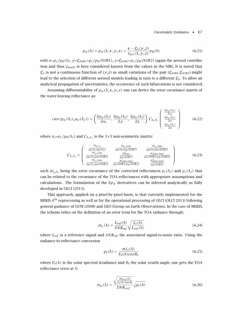
Uncertainty Estimates • 67
ρw(λ) = ρw(λ,x,y, z) =x − ζλ(y, z)td,v(λ,y, z)
ρR(λ) (4.21)
with x=ρc/ρR(λ), y=ζNIR1=ρc/ρR(NIR1), z=ζNIR2=ρc/ρR(NIR2) (again the aerosol contribu-
tion and thus ρpath is here considered known from the values in the NIR). It is noted that
ζλ is not a continuous function of (y ,z) as small variations of the pair (ζNIR1,ζNIR2) might
lead to the selection of different aerosol models leading in turn to a different ζλ. To allow an
analytical propagation of uncertainties, the occurrence of such bifurcations is not considered.
Assuming differentiability of ρw(λ,x,y, z) one can derive the error covariance matrix of
the water-leaving reflectance as:
cov(ρw(λi), ρw(λj)) =(∂ρw(λi)∂xi
,∂ρw(λi)∂y
,∂ρw(λi)∂z
)Cλi,λj
∂ρw(λj)∂xj
∂ρw(λj)∂y
∂ρw(λj)∂z
(4.22)
where xi=ρc/ρR(λi) and Cλi,λj is the 3×3 non-symmetric matrix:
Cλi,λj =
σλi,λj
ρR(λi)ρR(λj)σλi,NIR1
ρR(λi)ρR(NIR1)σλi,NIR2
ρR(λi)ρR(NIR2)σλj ,NIR1
ρR(λj)ρR(NIR1)σ2NIR1
ρ2R(NIR1)
σNIR1,NIR2
ρR(NIR1)ρR(NIR2)σλj ,NIR2
ρR(λj)ρR(NIR2)σNIR1,NIR2
ρR(NIR1)ρR(NIR2)σ2NIR1,NIR2
ρ2R(NIR2)
(4.23)
each σλi,λj being the error covariance of the corrected reflectances ρc(λi) and ρc(λj) that
can be related to the covariance of the TOA reflectances with appropriate assumptions and
calculations. The formulation of the ∂ρw derivatives can be inferred analytically as fully
developed in OLCI (2013).
This approach, applied on a pixel-by-pixel basis, is that currently implemented for the
MERIS 4th reprocessing as well as for the operational processing of OLCI (OLCI 2013) following
general guidance of GUM (2008) and GEO (Group on Earth Observations). In the case of MERIS,
the scheme relies on the definition of an error term for the TOA radiance through:
σLt (λ) =Lref (λ)SNRref
√Lt(λ)Lref (λ)
(4.24)
where Lref is a reference signal and SNRref the associated signal-to-noise ratio. Using the
radiance-to-reflectance conversion
ρt(λ) =πLt(λ)
F0(λ)cosθ0(4.25)
where F0(λ) is the solar spectral irradiance and θ0 the solar zenith angle, one gets the TOA
reflectance error at λ:
σρt (λ) =
√πLref (λ)F0(λ) cosθ0
SNRref
√ρt(λ) (4.26)
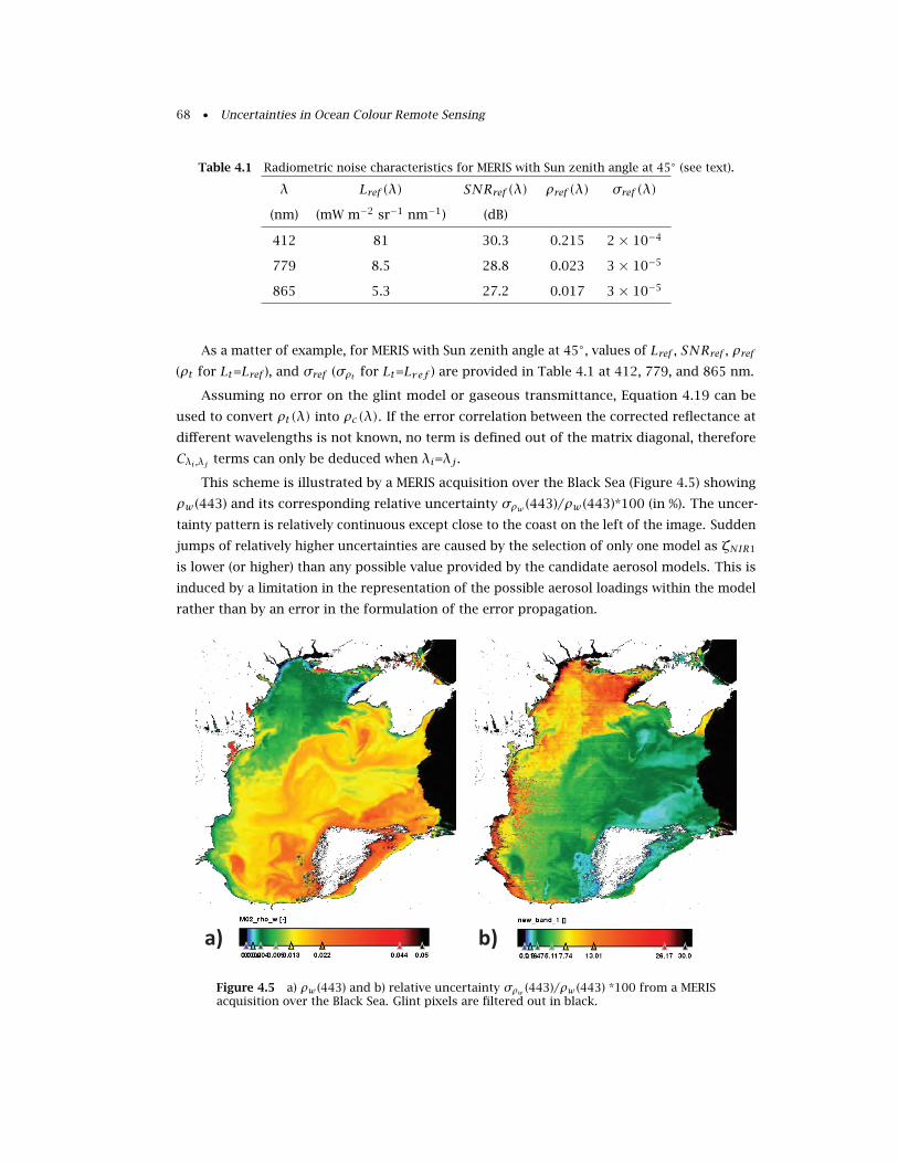
68 • Uncertainties in Ocean Colour Remote Sensing
Table 4.1 Radiometric noise characteristics for MERIS with Sun zenith angle at 45◦ (see text).
λ Lref (λ) SNRref (λ) ρref (λ) σref (λ)
(nm) (mW m−2 sr−1 nm−1) (dB)
412 81 30.3 0.215 2 × 10⁻⁴
779 8.5 28.8 0.023 3 × 10⁻⁵
865 5.3 27.2 0.017 3 × 10⁻⁵
As a matter of example, for MERIS with Sun zenith angle at 45◦, values of Lref , SNRref , ρref
(ρt for Lt=Lref ), and σref (σρt for Lt=Lref ) are provided in Table 4.1 at 412, 779, and 865 nm.
Assuming no error on the glint model or gaseous transmittance, Equation 4.19 can be
used to convert ρt(λ) into ρc(λ). If the error correlation between the corrected reflectance at
different wavelengths is not known, no term is defined out of the matrix diagonal, therefore
Cλi,λj terms can only be deduced when λi=λj .
This scheme is illustrated by a MERIS acquisition over the Black Sea (Figure 4.5) showing
ρw (443) and its corresponding relative uncertainty σρw (443)/ρw (443)*100 (in %). The uncer-
tainty pattern is relatively continuous except close to the coast on the left of the image. Sudden
jumps of relatively higher uncertainties are caused by the selection of only one model as ζNIR1
is lower (or higher) than any possible value provided by the candidate aerosol models. This is
induced by a limitation in the representation of the possible aerosol loadings within the model
rather than by an error in the formulation of the error propagation.
a) b)
Figure 4.5 a) ρw (443) and b) relative uncertainty σρw (443)/ρw (443) *100 from a MERISacquisition over the Black Sea. Glint pixels are filtered out in black.
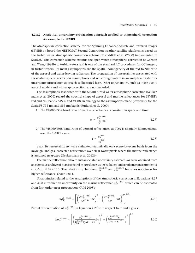
Uncertainty Estimates • 69
4.2.8.2 Analytical uncertainty-propagation approach applied to atmospheric correction:
An example for SEVIRI
The atmospheric correction scheme for the Spinning Enhanced Visible and Infrared Imager
(SEVIRI) on board the METEOSAT Second Generation weather satellite platform is based on
the turbid water atmospheric correction scheme of Ruddick et al. (2000) implemented in
SeaDAS. This correction scheme extends the open water atmospheric correction of Gordon
and Wang (1994b) to turbid waters and is one of the standard AC procedures for OC imagery
in turbid waters. Its main assumptions are the spatial homogeneity of the red-to-NIR ratio
of the aerosol and water-leaving radiances. The propagation of uncertainties associated with
these atmospheric correction assumptions and sensor digitization in an analytical first-order
uncertainty propagation approach is illustrated here. Other uncertainties, such as those due to
aerosol models and whitecap correction, are not included.
The assumptions associated with the SEVIRI turbid water atmospheric correction (Neuker-
mans et al. 2009) regard the spectral shape of aerosol and marine reflectances for SEVIRI’s
red and NIR bands, VIS06 and VIS08, in analogy to the assumptions made previously for the
SeaWiFS 765-nm and 865-nm bands (Ruddick et al. 2000):
1. The VIS06:VIS08 band ratio of marine reflectances is constant in space and time:
σ = ρ0+(0.6)w
ρ0+(0.8)w
(4.27)
2. The VIS06:VIS08 band ratio of aerosol reflectances at TOA is spatially homogeneous
over the SEVIRI scene:
ε = ρ(0.6)a
ρ(0.8)a(4.28)
ε and its uncertainty ∆ε were estimated statistically on a scene-by-scene basis from the
Rayleigh- and gas- corrected reflectances over clear water pixels where the marine reflectance
is assumed near-zero (Neukermans et al. 2012b).
The marine reflectance ratio σ and associated uncertainty estimate ∆σ were obtained from
an extensive archive of hyperspectral in situ above-water radiance and irradiance measurements,
σ ± ∆σ = 6.09±0.16. The relationship between ρ0+(0.8)w and ρ0+(0.6)
w becomes non-linear for
higher reflectance, above 0.011.
Uncertainties related to the assumptions of the atmospheric correction in Equations 4.27
and 4.28 introduce an uncertainty on the marine reflectance ρ0+(0.6)w , which can be estimated
from first-order error propagation (GUM 2008):
∆ρ0+(0.6)w =
(∂ρ0+(0.6)w
∂ε(6,8)∆ε)2
+(∂ρ0+(0.6)w
∂σ∆σ
)21/2
(4.29)
Partial differentiation of ρ0+(0.6)w in Equation 4.29 with respect to σ and ε gives:
∆ρ0+(0.6)w =
ρ0+(0.8)
w σta(0.8)0,v (γσ − ε)
∆ε
2
+(ρ0+(0.8)w εγσ − ε ∆σ
)2
1/2
(4.30)
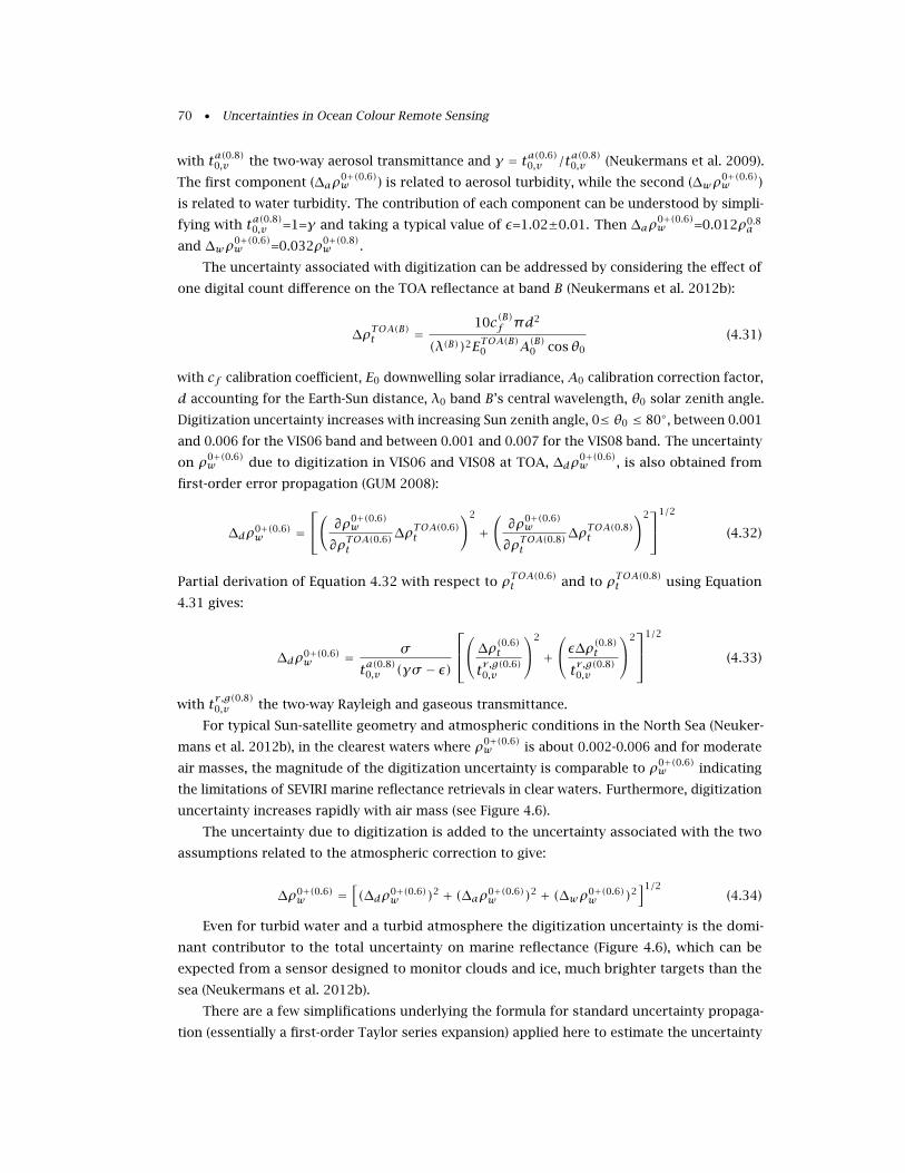
70 • Uncertainties in Ocean Colour Remote Sensing
with ta(0.8)0,v the two-way aerosol transmittance and γ = ta(0.6)0,v /ta(0.8)0,v (Neukermans et al. 2009).
The first component (∆aρ0+(0.6)w ) is related to aerosol turbidity, while the second (∆wρ
0+(0.6)w )
is related to water turbidity. The contribution of each component can be understood by simpli-
fying with ta(0.8)0,v =1=γ and taking a typical value of ε=1.02±0.01. Then ∆aρ0+(0.6)w =0.012ρ0.8
a
and ∆wρ0+(0.6)w =0.032ρ0+(0.8)
w .
The uncertainty associated with digitization can be addressed by considering the effect of
one digital count difference on the TOA reflectance at band B (Neukermans et al. 2012b):
∆ρTOA(B)t =10c(B)f πd2
(λ(B))2ETOA(B)0 A(B)0 cosθ0
(4.31)
with cf calibration coefficient, E0 downwelling solar irradiance, A0 calibration correction factor,
d accounting for the Earth-Sun distance, λ0 band B’s central wavelength, θ0 solar zenith angle.
Digitization uncertainty increases with increasing Sun zenith angle, 0≤ θ0 ≤ 80◦, between 0.001
and 0.006 for the VIS06 band and between 0.001 and 0.007 for the VIS08 band. The uncertainty
on ρ0+(0.6)w due to digitization in VIS06 and VIS08 at TOA, ∆dρ
0+(0.6)w , is also obtained from
first-order error propagation (GUM 2008):
∆dρ0+(0.6)w =
( ∂ρ0+(0.6)w
∂ρTOA(0.6)t∆ρTOA(0.6)t
)2
+(∂ρ0+(0.6)w
∂ρTOA(0.8)t∆ρTOA(0.8)t
)21/2
(4.32)
Partial derivation of Equation 4.32 with respect to ρTOA(0.6)t and to ρTOA(0.8)t using Equation
4.31 gives:
∆dρ0+(0.6)w = σ
ta(0.8)0,v (γσ − ε)
∆ρ(0.6)t
tr ,g(0.6)0,v
2
+ε∆ρ(0.8)t
tr ,g(0.8)0,v
2
1/2
(4.33)
with tr ,g(0.8)0,v the two-way Rayleigh and gaseous transmittance.
For typical Sun-satellite geometry and atmospheric conditions in the North Sea (Neuker-
mans et al. 2012b), in the clearest waters where ρ0+(0.6)w is about 0.002-0.006 and for moderate
air masses, the magnitude of the digitization uncertainty is comparable to ρ0+(0.6)w indicating
the limitations of SEVIRI marine reflectance retrievals in clear waters. Furthermore, digitization
uncertainty increases rapidly with air mass (see Figure 4.6).
The uncertainty due to digitization is added to the uncertainty associated with the two
assumptions related to the atmospheric correction to give:
∆ρ0+(0.6)w =
[(∆dρ0+(0.6)
w )2 + (∆aρ0+(0.6)w )2 + (∆wρ0+(0.6)
w )2]1/2
(4.34)
Even for turbid water and a turbid atmosphere the digitization uncertainty is the domi-
nant contributor to the total uncertainty on marine reflectance (Figure 4.6), which can be
expected from a sensor designed to monitor clouds and ice, much brighter targets than the
sea (Neukermans et al. 2012b).
There are a few simplifications underlying the formula for standard uncertainty propaga-
tion (essentially a first-order Taylor series expansion) applied here to estimate the uncertainty
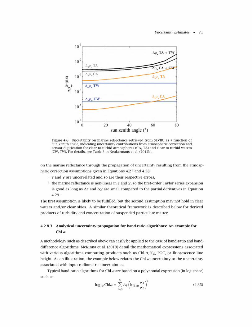
Uncertainty Estimates • 71
Figure 4.6 Uncertainty on marine reflectance retrieved from SEVIRI as a function ofSun zenith angle, indicating uncertainty contributions from atmospheric correction andsensor digitization for clear to turbid atmospheres (CA, TA) and clear to turbid waters(CW, TW). For details, see Table 3 in Neukermans et al. (2012b).
on the marine reflectance through the propagation of uncertainty resulting from the atmosp-
heric correction assumptions given in Equations 4.27 and 4.28:
◦ ε and γ are uncorrelated and so are their respective errors,
◦ the marine reflectance is non-linear in ε and γ, so the first-order Taylor series expansion
is good as long as ∆ε and ∆γ are small compared to the partial derivatives in Equation
4.29.
The first assumption is likely to be fulfilled, but the second assumption may not hold in clear
waters and/or clear skies. A similar theoretical framework is described below for derived
products of turbidity and concentration of suspended particulate matter.
4.2.8.3 Analytical uncertainty-propagation for band-ratio algorithms: An example for
Chl-a.
A methodology such as described above can easily be applied to the case of band-ratio and band-
difference algorithms. McKinna et al. (2019) detail the mathematical expressions associated
with various algorithms computing products such as Chl-a, Kd, POC, or fluorescence line
height. As an illustration, the example below relates the Chl-a uncertainty to the uncertainty
associated with input radiometric uncertainties.
Typical band-ratio algorithms for Chl-a are based on a polynomial expression (in log-space)
such as:
log10 Chla =N∑i=0
Ai(
log10R1
R2
)i(4.35)
72 • Uncertainties in Ocean Colour Remote Sensing
where R is a reflectance value, irradiance reflectance or remote sensing reflectance (O’Reilly
et al. 2000). In some cases, the input bands may vary (e.g., in maximum band-ratio algorithms),
but once they are selected, this is a two-band algorithm.
Assuming no bifurcation in the selection of the two bands (which would cause discon-
tinuities) and not considering model errors (i.e., making the strong assumption of negligible
uncertainties on the polynomial coefficients), an analytical derivation of Chl-a uncertainty
relative to the propagation of radiometric uncertainties can be derived through:
σ 2Chla = Chla2
N∑i=1
iAi(
log10R1
R2
)i−12 (
σ 2R1
R21
− 2σR1R2
R1R2+σ 2R2
R22
)(4.36)
where σR1R2 is the error covariance between reflectances R1 and R2.
This formula shows that the uncertainty on Chl-a is small when the errors of R1 and R2
are positively correlated. In the ideal case of a perfect correlation (admittedly an unrealistic
hypothesis), the uncertainty is minimal with:
σChla = Chla
∣∣∣∣∣∣N∑i=1
iAi(
log10R1
R2
)i−1∣∣∣∣∣∣
∣∣∣∣σR1
R1− σR2
R2
∣∣∣∣ (4.37)
when σR1R2 = σR1σR2 . The uncertainty vanishes if the input uncertainties have close relative
values (i.e.,σR1R1' σR2
R2). This highlights the known interest of band ratio algorithms to retrieve
ocean characteristics as ratios dampen the effect of radiometric errors.
For the same western Black Sea scene as Figure 4.5, Figure 4.7 shows Chl-a obtained from
the OC4Me algorithm used in the MERIS and OLCI processing chains (based on the reflectance
model of Morel and Maritorena 2001) and its associated uncertainty, which can reach about
10% of Chl-a (a low value that does not take into account model errors).
The error associated with Chl-a can be considerably higher if the errors affecting the
reflectance values take different signs, possibly reaching tens of percent when errors on
reflectance is only ±3% (Figure 4.8). In the same Case-1 water framework as above and with an
algorithm such as OC4v6 (O’Reilly et al. 2000), the error of Chl-a is minimal in the range of
concentrations 0.2-0.3 mg m−3 that happens to be close to the most frequent values found in
the oceans. In this theoretical exercise as well as above with the OC4Me algorithm, it is worth
repeating that uncertainties are considered to come only from the input quantity, implicitly
assuming a perfect algorithm.
Fortunately, errors of different signs in a band-ratio algorithm is a worst case scenario.
There is some ground suggesting that errors in R (or RRS ) have a degree of spectral correlation
(Hu et al. 2013; Section 4.3.1) which can be explained by the functioning of AC algorithms (for
instance as the estimate of aerosol radiance can affect the entire visible spectrum). So part of
these errors might be cancelled in Chl-a band-ratio algorithms. For the same reason, these
errors are almost completely eliminated in a band-difference OCI algorithm (Hu et al. 2012b),
making the OCI Chl-a nearly free of these RRS errors regardless of the magnitude of Chl-a
for Chl-a < 0.25 mg m−3 (again assuming no model errors). Similarly, using the same error
propagation principles, Qi et al. (2017b) showed much lower uncertainties in Chl-a obtained by
a band-difference algorithm than those derived from a band ratio.
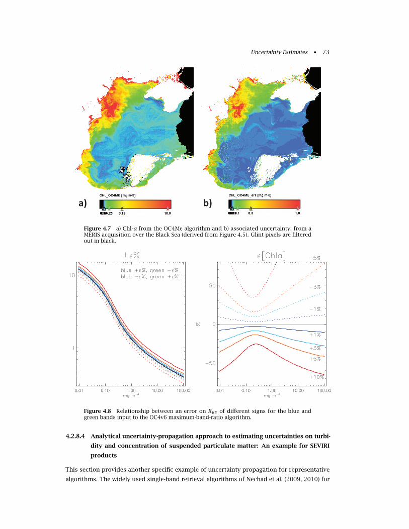
Uncertainty Estimates • 73
a) b)
Figure 4.7 a) Chl-a from the OC4Me algorithm and b) associated uncertainty, from aMERIS acquisition over the Black Sea (derived from Figure 4.5). Glint pixels are filteredout in black.
Figure 4.8 Relationship between an error on RRS of different signs for the blue andgreen bands input to the OC4v6 maximum-band-ratio algorithm.
4.2.8.4 Analytical uncertainty-propagation approach to estimating uncertainties on turbi-
dity and concentration of suspended particulate matter: An example for SEVIRI
products
This section provides another specific example of uncertainty propagation for representative
algorithms. The widely used single-band retrieval algorithms of Nechad et al. (2009, 2010) for
74 • Uncertainties in Ocean Colour Remote Sensing
turbidity and suspended particulate matter concentration [SPM] are, respectively:
T = ATρ0+(0.6)w
C − ρ0+(0.6)w
+ BT (4.38)
[SPM] = ASρ0+(0.6)w
C − ρ0+(0.6)w
+ BS (4.39)
where C is band specific, giving C=0.1639 for the SEVIRI VIS06 band. The coefficients (AT ,
BT ) of the turbidity algorithm and (AS , BS ) of the [SPM] algorithm are derived from non-
linear regression of 68 in situ observations of marine reflectance and T or [SPM] obtained
in the southern North Sea in 2007-2010 (see Nechad et al. 2010, for details on curve fitting).
Regression gives coefficients with standard error AT=35.8±3.8 FNU and BT=-0.1±0.9 FNU for
the T algorithm and AS= 37.1±5.7 mg L−1 and BS= -0.17±1.4 mg L−1 for the [SPM] algorithm.
The offsets BT and BS not being significantly different from zero, the T and [SPM] algorithms
are applied without them.
The uncertainty on the retrieval of T or [SPM] using algorithms of the form 4.38/4.39
resulting from uncertainties on ρ0+(0.6)w and their respective calibration parameters, AT or AS ,
is estimated from first-order uncertainty propagation (GUM 2008) to give:
∆T = 1
C − ρ0+(0.6)w
(ATC∆ρ0+(0.6)w
C − ρ0+(0.6)w
)2
+(ρ0+(0.6)w ∆AT
)2
1/2
(4.40)
This expression can be written analogously for the uncertainty on [SPM], denoted ∆S, by
replacing AT with AS . The relative uncertainty on turbidity can be expressed as follows:
∆TT=( CC − ρ0+(0.6)
w
∆ρ0+(0.6)w
ρ0+(0.6)w
)2
+(∆ATAT
)21/2
(4.41)
where ∆ATAT =0.11. For [SPM], ∆AS
AS =0.15. The two components in Equation 4.41 are of very
different nature. The first component is related to the uncertainty on marine reflectance due
to atmospheric correction and sensor issues like digitization, where the latter is the dominant
source of uncertainty for SEVIRI (see above). The second component is the uncertainty arising
from the calibration of the retrieval algorithms for T and [SPM] and is equal to 11% and 15%,
respectively, everywhere in the scene. Uncertainties in the [SPM] and T algorithm calibration
are caused by various factors such as in situ measurement uncertainties for reflectance, T , and
[SPM] and uncertainties in the optical model underlying Equations 4.38 and 4.39. As discussed
in Nechad et al. (2010), the main source of uncertainty in the T and [SPM] algorithms is the
natural variability of the turbidity- and mass-specific backscattering ratios (Neukermans et al.
2012a), respectively. Depending on the water constituents, these values might have a strong
regional character (associated with natural variability in the relationship between [SPM] and
IOPs) that might necessitate the recalibration of the algorithms (Equations 4.38 and 4.39) in
different regions.
Uncertainty Estimates • 75
4.2.8.5 Analytical uncertainty-propagation approach to estimating IOPs: An example with
the QAA
A similar approach for uncertainties can be applied to bio-optical algorithms based on an
analytical formulation, which is the case of the Quasi-Analytical Algorithm (QAA, Lee et al.
2002). The main input to the QAA is the below-water remote sensing reflectance rrs , writing
(see Section 3.2.7):
rrs(λ) = g0u(λ)+ g1u2(λ) (4.42)
with u=bb/(bb+a) with bb and a being the total backscattering and absorption coefficients,
respectively. The QAA is based on the assumptions: i) total absorption can be derived at a
reference wavelength λ0 (typically around or above 550 nm) where the non-water absorption
coefficient is considered low and without a strong variability (Lee et al. 2002), ii) the spectral
shape of the particulate backscattering coefficient follows a power law of exponent η:
bbp(λ) = bbp(λ0)(λ0
λ
)η(4.43)
In the QAA, both a(λ0) and η are derived from the rrs spectrum using empirical relations-
hips. From Equation 4.42, knowing rrs(λ0) and a(λ0), bbp(λ0) is easily computed, as is bbp(λ)from Equation 4.43. Then from Equation 4.42 again, a(λ) can be derived at all wavelengths.
Adopting an analytical scheme of uncertainty propagation with first-order derivatives
(GUM 2008), Lee et al. (2010) have derived an expression for the uncertainties associated with
a(λ) and bbp(λ) assuming that the uncertainties on rrs can be neglected. In that case, and
noting B=u/(1-u), the uncertainty on bbp and a can be written as:
∆bbp(λ0) = B(λ0)∆a(λ0) (4.44)
∆bbp(λ) =
√√√√(B(λ0)(λ0
λ
)η∆a(λ0)
)2
+([B(λ0)a(λ0)− bbw(λ0)]
(λ0
λ
)ηln(λ0
λ
)∆η)2
(4.45)
∆a(λ) =
√√√√(B(λ0
B(λ)
(λ0
λ
)η∆a(λ0)
)2
+(
1B(λ)
[B(λ0)a(λ0)− bbw(λ0)](λ0
λ
)ηln(λ0
λ
)∆η)2
(4.46)
where ∆a(λ0) and ∆η are the uncertainties associated with a(λ0) and η, respectively. In Lee
et al. (2010), the uncertainty on a(λ0) (λ0 with equal to 547 nm) was estimated from the
distribution of differences between true value and QAA output using a synthetic data set, with
the conclusion that for a(λ0) <0.1 m−1, the difference (in relative terms) is generally less than
16%. This could lead to an uncertainty for bbp(λ0) of approximately 10%. The uncertainty ∆ηwas assumed equal to the conservative (fairly high) value of 0.5. From these definitions, the
uncertainty associated with a can be computed, found usually within 10% for a(443) for low
76 • Uncertainties in Ocean Colour Remote Sensing
absorption waters (a(443) less than 0.05 m−1). ∆a(443)/a(443) increases noticeably for higher
absorption values and the weight of ∆a(λ0) becomes predominant with respect to ∆η.
Total absorption can be further decomposed into components due to phytoplankton aph
and detrital material acdm. The QAA performs that step analytically assuming known the ratios
ζ=aph(λ1)/aph(λ2) and ξ=acdm(λ1)/acdm(λ2) where typically λ1 and λ2 are 412 and 443 nm,
respectively. The assumption about the latter term is equivalent to defining the exponential
slope (and the spectral shape) of acdm. Thus, the uncertainties on the IOPs aph and acdmcan be expressed as a function of ∆a(λ0), ∆η, ∆ζ and ∆ξ and, not surprisingly, they can be
noticeably higher than for total absorption. The formula given in Lee et al. (2010) obtained
for aph and acdm highlight the complexity of deriving uncertainty estimates for IOPs, which
could be further compounded if additional sources of uncertainty were taken into account,
principally from rrs as well as from bio-optical modelling assumptions.
4.2.9 Uncertainty propagation using a Monte-Carlo approach
Ensemble-type methods, such as Monte Carlo (also referred to as bootstrap), provide another
technique for estimating uncertainties in non-linearly derived OC products. Briefly, this
requires perturbing each input reflectance and/or the inverse model parameterization m times,
thus returning a set of m candidate solutions. The distribution of candidate solutions then
provides both the optimal solution (via, e.g., the mean or median of the distribution), as well
as the associated uncertainties (via, e.g., the standard deviation of the distribution). In the
case of the parameterization of a bio-optical algorithm, the basic idea is simple: since inputs
into an algorithm (RRS and the spectral shape of IOPs assumed in the model) always suffer
from uncertainties, rather than solving a single inversion we sample thousands of inversions
each using inputs ± their likely uncertainties. The statistics of the ensemble solutions then
provide information on the likely solution and its uncertainty. This approach assumes the
uncertainties in the inputs and their statistics are known.
A demonstration of this concept on RRS non-linear inversions (both field-data and simula-
ted data) was performed by Wang et al. (2005) and Boss and Roessler (IOCCG 2006, Chapter
8). A standard semi-analytical approach was used where the IOPs were allowed to vary in
shape (absorption by non-algal particles and CDOM, bbp and aph all had 11 types for shapes).
Since under this framework the RRS -IOP relationship can be written as a simple matrix for all
wavelengths, the linear inversion assures a single best solution (in a least-square sense) for
each assumed set of IOP shapes. All solutions satisfying being within 5% of RRS were kept
and their statistics were used to compute the most likely value of a parameter and its uncer-
tainties. Interestingly, concentration parameters (e.g., Chl-a) were retrieved with acceptable
uncertainties while shape parameters (e.g., size parameter associated with aph) were most
often not. Similarly, Salama (2012) used an ensemble-based approach to quantify inherent
optical property uncertainties in a stochastic inverse models.
A similar concept has been applied for an analysis of an atmospheric correction scheme
(NASA standard algorithm), taking into account the noise associated with top-of-atmosphere
radiance Lt for the SeaWiFS instrument (Franz and Karaköylü 2016). Each TOA Lt datum
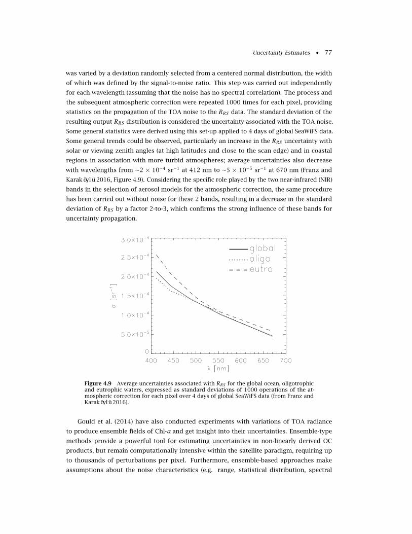
Uncertainty Estimates • 77
was varied by a deviation randomly selected from a centered normal distribution, the width
of which was defined by the signal-to-noise ratio. This step was carried out independently
for each wavelength (assuming that the noise has no spectral correlation). The process and
the subsequent atmospheric correction were repeated 1000 times for each pixel, providing
statistics on the propagation of the TOA noise to the RRS data. The standard deviation of the
resulting output RRS distribution is considered the uncertainty associated with the TOA noise.
Some general statistics were derived using this set-up applied to 4 days of global SeaWiFS data.
Some general trends could be observed, particularly an increase in the RRS uncertainty with
solar or viewing zenith angles (at high latitudes and close to the scan edge) and in coastal
regions in association with more turbid atmospheres; average uncertainties also decrease
with wavelengths from ∼2 × 10⁻⁴ sr−1 at 412 nm to ∼5 × 10⁻⁵ sr−1 at 670 nm (Franz and
Karaköylü 2016, Figure 4.9). Considering the specific role played by the two near-infrared (NIR)
bands in the selection of aerosol models for the atmospheric correction, the same procedure
has been carried out without noise for these 2 bands, resulting in a decrease in the standard
deviation of RRS by a factor 2-to-3, which confirms the strong influence of these bands for
uncertainty propagation.
Figure 4.9 Average uncertainties associated with RRS for the global ocean, oligotrophicand eutrophic waters, expressed as standard deviations of 1000 operations of the at-mospheric correction for each pixel over 4 days of global SeaWiFS data (from Franz andKaraköylü 2016).
Gould et al. (2014) have also conducted experiments with variations of TOA radiance
to produce ensemble fields of Chl-a and get insight into their uncertainties. Ensemble-type
methods provide a powerful tool for estimating uncertainties in non-linearly derived OC
products, but remain computationally intensive within the satellite paradigm, requiring up
to thousands of perturbations per pixel. Furthermore, ensemble-based approaches make
assumptions about the noise characteristics (e.g. range, statistical distribution, spectral
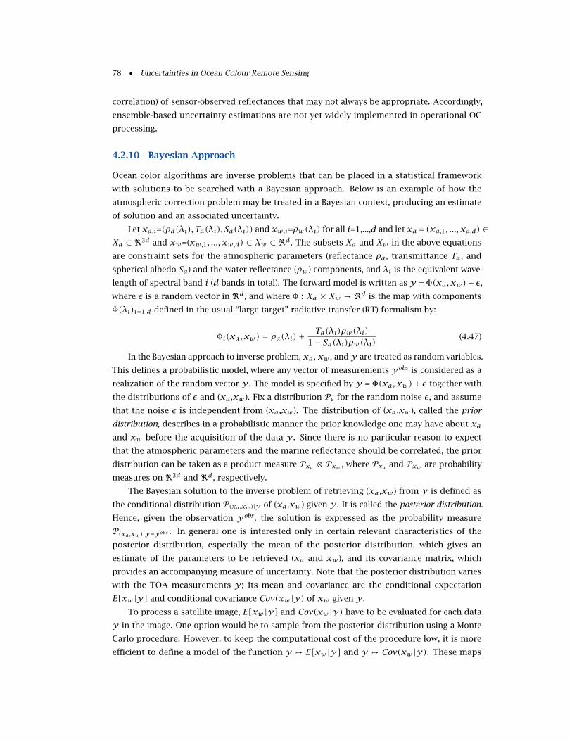
78 • Uncertainties in Ocean Colour Remote Sensing
correlation) of sensor-observed reflectances that may not always be appropriate. Accordingly,
ensemble-based uncertainty estimations are not yet widely implemented in operational OC
processing.
4.2.10 Bayesian Approach
Ocean color algorithms are inverse problems that can be placed in a statistical framework
with solutions to be searched with a Bayesian approach. Below is an example of how the
atmospheric correction problem may be treated in a Bayesian context, producing an estimate
of solution and an associated uncertainty.
Let xa,i=(ρa(λi), Ta(λi), Sa(λi)) and xw,i=ρw(λi) for all i=1,...,d and let xa = (xa,1, ..., xa,d) ∈Xa ⊂ <3d and xw=(xw,1, ..., xw,d) ∈ Xw ⊂ <d. The subsets Xa and Xw in the above equations
are constraint sets for the atmospheric parameters (reflectance ρa, transmittance Ta, and
spherical albedo Sa) and the water reflectance (ρw ) components, and λi is the equivalent wave-
length of spectral band i (d bands in total). The forward model is written as y = Φ(xa, xw) + ε,where ε is a random vector in <d, and where Φ : Xa × Xw → <d is the map with components
Φ(λi)i=1,d defined in the usual “large target” radiative transfer (RT) formalism by:
Φi(xa, xw) = ρa(λi)+Ta(λi)ρw(λi)
1− Sa(λi)ρw(λi)(4.47)
In the Bayesian approach to inverse problem, xa, xw , and y are treated as random variables.
This defines a probabilistic model, where any vector of measurements yobs is considered as a
realization of the random vector y . The model is specified by y = Φ(xa, xw) + ε together with
the distributions of ε and (xa,xw ). Fix a distribution Pε for the random noise ε, and assume
that the noise ε is independent from (xa,xw ). The distribution of (xa,xw ), called the prior
distribution, describes in a probabilistic manner the prior knowledge one may have about xaand xw before the acquisition of the data y . Since there is no particular reason to expect
that the atmospheric parameters and the marine reflectance should be correlated, the prior
distribution can be taken as a product measure Pxa ⊗ Pxw , where Pxa and Pxw are probability
measures on <3d and <d, respectively.
The Bayesian solution to the inverse problem of retrieving (xa,xw ) from y is defined as
the conditional distribution P(xa,xw)|y of (xa,xw ) given y . It is called the posterior distribution.
Hence, given the observation yobs , the solution is expressed as the probability measure
P(xa,xw)|y=yobs . In general one is interested only in certain relevant characteristics of the
posterior distribution, especially the mean of the posterior distribution, which gives an
estimate of the parameters to be retrieved (xa and xw ), and its covariance matrix, which
provides an accompanying measure of uncertainty. Note that the posterior distribution varies
with the TOA measurements y ; its mean and covariance are the conditional expectation
E[xw |y] and conditional covariance Cov(xw |y) of xw given y .
To process a satellite image, E[xw |y] and Cov(xw |y) have to be evaluated for each data
y in the image. One option would be to sample from the posterior distribution using a Monte
Carlo procedure. However, to keep the computational cost of the procedure low, it is more
efficient to define a model of the function y , E[xw |y] and y , Cov(xw |y). These maps
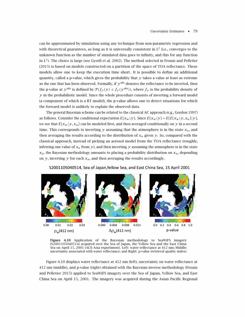
Uncertainty Estimates • 79
can be approximated by simulation using any technique from non-parametric regression and
with theoretical guarantees, as long as it is universally consistent in L2 (i.e., converges to the
unknown function as the number of simulated data goes to infinity, and this for any function
in L2). The choice is large (see Gyorfi et al. 2002). The method selected in Frouin and Pelletier
(2015) is based on models constructed on a partition of the space of TOA reflectance. These
models allow one to keep the execution time short. It is possible to define an additional
quantity, called a p-value, which gives the probability that y takes a value at least as extreme
as the one that has been observed. Formally, if yobs denotes the reflectance to be inverted, then
the p-value at yobs is defined by P(fy(y) ≤ fy(yobs)), where fy is the probability density of
y in the probabilistic model. Since the whole procedure consists of inverting a forward model
(a component of which is a RT model), the p-value allows one to detect situations for which
the forward model is unlikely to explain the observed data.
The general Bayesian scheme can be related to the classical AC approach (e.g., Gordon 1997)
as follows. Consider the conditional expectation E[xw |y]. Since E[xw |y] = E[E[xw |y,xa]|y],we see that E[xw |y,xa] can be modeled first, and then averaged conditionally on y in a second
time. This corresponds to inverting y assuming that the atmosphere is in the state xa, and
then averaging the results according to the distribution of xa given y . So, compared with the
classical approach, instead of picking an aerosol model from the TOA reflectance (roughly,
inferring one value of xa from y), and then inverting y assuming the atmosphere is in the state
xa, the Bayesian methodology amounts to placing a probability distribution on xa, depending
on y , inverting y for each xa, and then averaging the results accordingly.
Figure 4.10 Application of the Bayesian methodology to SeaWiFS imagery(S2001105040514) acquired over the Sea of Japan, the Yellow Sea and the East ChinaSea on April 15, 2001 (ACE-Asia experiment). Left: water reflectance at 412 nm; Middle:uncertainty associated with water reflectance; and Right: p-value (retrieval quality index).
Figure 4.10 displays water reflectance at 412 nm (left), uncertainty on water reflectance at
412 nm (middle), and p-value (right) obtained with the Bayesian inverse methodology (Frouin
and Pelletier 2015) applied to SeaWiFS imagery over the Sea of Japan, Yellow Sea, and East
China Sea on April 15, 2001. The imagery was acquired during the Asian Pacific Regional
80 • Uncertainties in Ocean Colour Remote Sensing
Characterization Experiment (ACE-Asia). The atmosphere contained a variety of aerosols,
including wind-blown dust from the China deserts and particles generated by human activity
and industrial sources (Kahn et al. 2004). The water reflectance at 412 nm exhibits low values
(0.005 to 0.015) in the Sea of Japan, where waters are generally productive, and relatively high
values in the East China Sea, due to sediments from the Yangtze River. The retrieval shows
good spatial continuity, but abnormal values are sometimes encountered in the vicinity of
clouds. Larger uncertainties are generally associated with abnormal water reflectance values.
In the clear sky region between Korea and Japan, uncertainties are also high (> 0.01), which is
due to absorbing aerosols (polluted air and dust from Yellow Sea, North China, and Northeast
Mongolia, see Kahn et al. 2004), and the likely inability of the forward model to represent local
aerosol conditions, especially the effect of aerosol altitude on the aerosol reflectance. Note that
the uncertainties are quite small (0.003–0.004) in the region influenced by the Yangtze River,
even though the optically complex waters in that region are not represented in the forward
model. Such situations may occur, for which part of the marine signal, generally not null
in the near infrared, is interpreted as an aerosol signal, resulting in a posterior probability
distribution with small conditional covariance. This suggests that the conditional covariance is
not a sufficient measure of uncertainty. One needs to take into consideration the adequacy of
the forward model to fit the observations, or the probability that the model takes values as
extreme as the observations, i.e., the p-value, in the assessment of performance. In many parts
of the imagery, the p-value is above 0.5, indicating good compatibility between model and
observations. In the vicinity of clouds, or in non-cloudy regions affected by absorbing aerosols
(Sea of Japan, Korea Strait), the p-values are relatively low, yet acceptable (> 0.1). Unacceptable
values (< 0.05) are encountered in the East China Sea. In these regions, model and observations
are inconsistent, and the retrievals should be rejected, even though the conditional covariance
may be low.
4.2.11 Use of Cramér-Rao Bounds
The uncertainty in a given OC product has several components, each of which arises from
a particular stage of the whole calibration, measurement and processing chain. While all of
these components must be included when evaluating the total uncertainty budget for a given
product, it is also useful to quantify the influence of each component separately in order
to determine which source(s) of uncertainty has (have) the greatest impact on estimation
performance and should be treated first. For example, when computing the experimental
estimation variance obtained by applying a given algorithm to some simulated remote-sensing
data, one only takes into account the uncertainties related to the bio-optical and noise models,
the sensor radiometric configuration and the inverse method. However, this approach may be
computationally expensive, and one cannot know to what extent the obtained uncertainties
could be improved using another algorithm.
Recently, a statistical technique based on Cramér-Rao bounds (CRBs) has been applied to
OC remote sensing, directly providing algorithm-independent uncertainties while not requiring
any inversion (Jay et al. 2018). This theoretical tool actually provides the minimum estimation
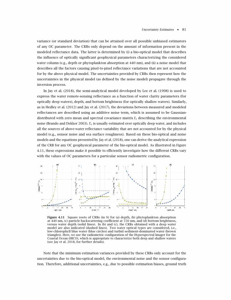
Uncertainty Estimates • 81
variance (or standard deviation) that can be attained over all possible unbiased estimators
of any OC parameter. The CRBs only depend on the amount of information present in the
modeled reflectance data. The latter is determined by (i) a bio-optical model that describes
the influence of optically significant geophysical parameters characterizing the considered
water column (e.g., depth or phytoplankton absorption at 440 nm), and (ii) a noise model that
describes all the factors causing pixel-to-pixel reflectance variations that are not accounted
for by the above physical model. The uncertainties provided by CRBs then represent how the
uncertainties in the physical model (as defined by the noise model) propagate through the
inversion process.
In Jay et al. (2018), the semi-analytical model developed by Lee et al. (1998) is used to
express the water remote-sensing reflectance as a function of water clarity parameters (for
optically deep waters), depth, and bottom brightness (for optically shallow waters). Similarly,
as in Hedley et al. (2012) and Jay et al. (2017), the deviations between measured and modeled
reflectances are described using an additive noise term, which is assumed to be Gaussian-
distributed with zero mean and spectral covariance matrix Γs describing the environmental
noise (Brando and Dekker 2003). Γs is usually estimated over optically deep water, and includes
all the sources of above-water reflectance variability that are not accounted for by the physical
model (e.g., sensor noise and sea surface roughness). Based on these bio-optical and noise
models and the equations presented by Jay et al. (2018), one can derive the analytical expression
of the CRB for any OC geophysical parameter of the bio-optical model. As illustrated in Figure
4.11, these expressions make it possible to efficiently investigate how the different CRBs vary
with the values of OC parameters for a particular sensor radiometric configuration.
Figure 4.11 Square roots of CRBs (in %) for (a) depth, (b) phytoplankton absorptionat 440 nm, (c) particle backscattering coefficient at 550 nm, and (d) bottom brightness,versus water depth (solid lines). In (b) and (c), the CRBs obtained with a deep watermodel are also indicated (dashed lines). Two water optical types are considered, i.e.,low-chlorophyll blue water (blue circles) and turbid sediment-dominated water (browntriangles). Here, we use the radiometric configuration of the Hyperspectral Imager for theCoastal Ocean (HICO), which is appropriate to characterize both deep and shallow waters(see Jay et al. 2018, for further details).
Note that the minimum estimation variances provided by these CRBs only account for the
uncertainties due to the bio-optical model, the environmental noise and the sensor configura-
tion. Therefore, additional uncertainties, e.g., due to possible estimation biases, ground truth
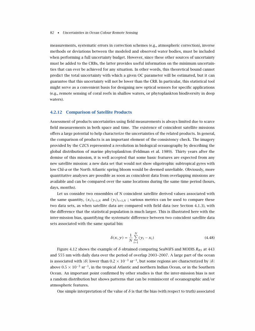
82 • Uncertainties in Ocean Colour Remote Sensing
measurements, systematic errors in correction schemes (e.g., atmospheric correction), inverse
methods or deviations between the modeled and observed water bodies, must be included
when performing a full uncertainty budget. However, since these other sources of uncertainty
must be added to the CRBs, the latter provides useful information on the minimum uncertain-
ties that can ever be achieved for any situation. In other words, this theoretical bound cannot
predict the total uncertainty with which a given OC parameter will be estimated, but it can
guarantee that this uncertainty will not be lower than the CRB. In particular, this statistical tool
might serve as a convenient basis for designing new optical sensors for specific applications
(e.g., remote sensing of coral reefs in shallow waters, or phytoplankton biodiversity in deep
waters).
4.2.12 Comparison of Satellite Products
Assessment of products uncertainties using field measurements is always limited due to scarce
field measurements in both space and time. The existence of coincident satellite missions
offers a large potential to help characterize the uncertainties of the related products. In general,
the comparison of products is an important element of the consistency check. The imagery
provided by the CZCS represented a revolution in biological oceanography by describing the
global distribution of marine phytoplankton (Feldman et al. 1989). Thirty years after the
demise of this mission, it is well accepted that some basic features are expected from any
new satellite mission: a new data set that would not show oligotrophic subtropical gyres with
low Chl-a or the North Atlantic spring bloom would be deemed unreliable. Obviously, more
quantitative analyses are possible as soon as coincident data from overlapping missions are
available and can be compared over the same locations during the same time period (hours,
days, months).
Let us consider two ensembles of N coincident satellite derived values associated with
the same quantity, (xi)i=1,N and (yi)i=1,N ; various metrics can be used to compare these
two data sets, as when satellite data are compared with field data (see Section 4.1.3), with
the difference that the statistical population is much larger. This is illustrated here with the
inter-mission bias, quantifying the systematic difference between two coincident satellite data
sets associated with the same spatial bin:
δ(x,y) = 1N
N∑i=1
(yi − xi) (4.48)
Figure 4.12 shows the example of δ obtained comparing SeaWiFS and MODIS RRS at 443
and 555 nm with daily data over the period of overlap 2003–2007. A large part of the ocean
is associated with |δ| lower than 0.2 × 10⁻³ sr−1, but some regions are characterized by |δ|above 0.5 × 10⁻³ sr−1, in the tropical Atlantic and northern Indian Ocean, or in the Southern
Ocean. An important point confirmed by other studies is that the inter-mission bias is not
a random distribution but shows patterns that can be reminiscent of oceanographic and/or
atmospheric features.
One simple interpretation of the value of δ is that the bias (with respect to truth) associated
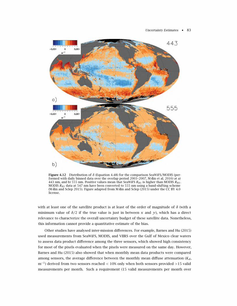
Uncertainty Estimates • 83
Figure 4.12 Distribution of δ (Equation 4.48) for the comparison SeaWiFS/MODIS (per-formed with daily binned data over the overlap period 2003–2007, Mélin et al. 2016) at a)443 nm, and b) 555 nm. Positive values mean that SeaWiFS RRS is higher than MODIS RRS .MODIS RRS data at 547 nm have been converted to 555 nm using a band-shifting scheme(Mélin and Sclep 2015). Figure adapted from Mélin and Sclep (2015) under the CC BY 4.0license.
with at least one of the satellite product is at least of the order of magnitude of δ (with a
minimum value of δ/2 if the true value is just in between x and y), which has a direct
relevance to characterize the overall uncertainty budget of these satellite data. Nonetheless,
this information cannot provide a quantitative estimate of the bias.
Other studies have analysed inter-mission differences. For example, Barnes and Hu (2015)
used measurements from SeaWiFS, MODIS, and VIIRS over the Gulf of Mexico clear waters
to assess data product difference among the three sensors, which showed high consistency
for most of the pixels evaluated when the pixels were measured on the same day. However,
Barnes and Hu (2015) also showed that when monthly mean data products were compared
among sensors, the average difference between the monthly mean diffuse attenuation (Kd,
m−1) derived from two sensors reached < 10% only when both sensors provided >15 valid
measurements per month. Such a requirement (15 valid measurements per month over
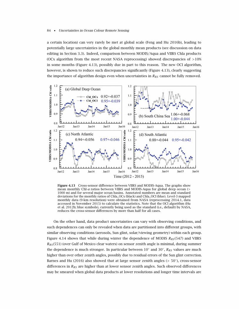
84 • Uncertainties in Ocean Colour Remote Sensing
a certain location) can very rarely be met at global scale (Feng and Hu 2016b), leading to
potentially large uncertainties in the global monthly mean products (see discussion on data
editing in Section 3.3). Indeed, comparison between MODIS/Aqua and VIIRS Chla products
(OCx algorithm from the most recent NASA reprocessing) showed discrepancies of >10%
in some months (Figure 4.13), possibly due in part to this reason. The new OCI algorithm,
however, is shown to reduce such discrepancies significantly (Figure 4.13), clearly suggesting
the importance of algorithm design even when uncertainties in RRS cannot be fully removed.
Figure 4.13 Cross-sensor difference between VIIRS and MODIS-Aqua. The graphs showmean monthly Chl-a ratios between VIIRS and MODIS-Aqua for global deep ocean (>1000 m) and for several major ocean basins. Annotated numbers are mean and standarddeviations for the monthly ratios of Chla_OCx (black) and Chla_OCI (blue). Level-3 mappedmonthly data (9-km resolution) were obtained from NASA (reprocessing 2014.1, dataaccessed in November 2015) to calculate the statistics. Note that the OCI algorithm (Huet al. 2012b; blue symbols), currently being used as the standard (i.e., default) by NASA,reduces the cross-sensor differences by more than half for all cases.
On the other hand, data product uncertainties can vary with observing conditions, and
such dependences can only be revealed when data are partitioned into different groups, with
similar observing conditions (aerosols, Sun glint, solar/viewing geometry) within each group.
Figure 4.14 shows that while during winter the dependence of MODIS RRS (547) and VIIRS
RRS (551) (over Gulf of Mexico clear waters) on sensor zenith angle is minimal, during summer
the dependence is much stronger. In particular between 10◦ and 30◦, RRS values are much
higher than over other zenith angles, possibly due to residual errors of the Sun glint correction.
Barnes and Hu (2016) also showed that at large sensor zenith angles (> 50◦), cross-sensor
differences in RRS are higher than at lower sensor zenith angles. Such observed differences
may be smeared when global data products at lower resolutions and longer time intervals are
Uncertainty Estimates • 85
evaluated.
Figure 4.14 RRS products in the green band from MODIS-Aqua (547 nm) and VIIRS(551 nm), both converted to 555 nm, over clear waters show dependency on sensorzenith angle during summer due to sun glint. The sensor performance and cross-sensorconsistency have been detailed in Barnes and Hu (2015, 2016). Figure adapted fromBarnes and Hu (2015) with permission from Elsevier.
As said above, comparison of satellite products, although it does not give uncertainty
estimates per se, is a large source of information, providing coincident data at high resolu-
tion across the full annual cycle and across the global ocean, at least in the parts regularly
covered by valid OC data. In a future when each OC datum is accompanied by an uncertainty
estimate, comparison between different products can be done in the context of compatibility,
as introduced in Chapter 2, with data expected to agree within their stated uncertainties.
4.2.13 Co-location Techniques
The availability of coincident satellite data can also provide quantitative information through
colocation techniques. Colocation is applied to derive uncertainty estimates in a variety of
Earth sciences, including oceanography (e.g., Stoffelen, 1998) or atmospheric sciences (e.g.,
Toohey and Strong 2001), and in the field of ocean colour it has been applied to Chl-a and RRSglobal distributions (Mélin 2010; Mélin et al. 2016).
Colocation techniques can be applied as soon as two ensembles of N coincident data are
available. Assuming that x and y can be modeled linearly as a function of a reference state rand zero-mean random errors, ε and ξ:
xi = ri + εi (4.49)
yi = α+ βri + ξi (4.50)
where α and β are the additive and multiplicative biases, respectively. Another assumption
is that ε and ξ are uncorrelated and independent of r (implying that all covariance terms
involving ε or ξ are null). The reference state r only serves to relate the two data sets being
analyzed: ideally, r should then be related to the true state in order to complete the uncertainty
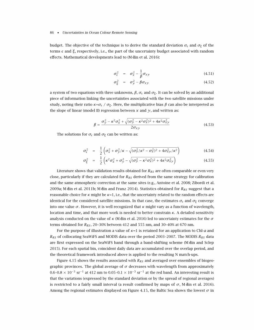
86 • Uncertainties in Ocean Colour Remote Sensing
budget. The objective of the technique is to derive the standard deviation σε and σξ of the
terms ε and ξ, respectively, i.e., the part of the uncertainty budget associated with random
effects. Mathematical developments lead to (Mélin et al. 2016):
σ 2ε = σ 2
x −1βσxy (4.51)
σ 2ξ = σ 2
y − βσxy (4.52)
a system of two equations with three unknowns, β, σε and σξ . It can be solved by an additional
piece of information linking the uncertainties associated with the two satellite missions under
study, noting their ratio κ=σε / σξ . Here, the multiplicative bias β can also be interpreted as
the slope of linear (model II) regression between x and y , and written as:
β =σ 2y − κ2σ 2
x +√(σ 2y − κ2σ 2
x)2 + 4κ2σ 2xy
2σxy(4.53)
The solutions for σε and σξ can be written as:
σ 2ε = 1
2
(σ 2x + σ 2
y/κ −√(σ 2y/κ2 − σ 2
x)2 + 4σ 2xy/κ2
)(4.54)
σ 2ξ = 1
2
(κ2σ 2
x + σ 2y −
√(σ 2y − κ2σ 2
x)2 + 4κ2σ 2xy
)(4.55)
Literature shows that validation results obtained for RRS are often comparable or even very
close, particularly if they are calculated for RRS derived from the same strategy for calibration
and the same atmospheric correction at the same sites (e.g., Antoine et al. 2008; Zibordi et al.
2009a; Mélin et al. 2011b; Mélin and Franz 2014). Statistics obtained for RRS suggest that a
reasonable choice for κ might be κ=1, i.e., that the uncertainty related to the random effects are
identical for the considered satellite missions. In that case, the estimates σε and σξ converge
into one value σ . However, it is well recognized that κ might vary as a function of wavelength,
location and time, and that more work is needed to better constrain κ. A detailed sensitivity
analysis conducted on the value of κ (Mélin et al. 2016) led to uncertainty estimates for the σterms obtained for RRS , 20–30% between 412 and 555 nm, and 30–40% at 670 nm.
For the purpose of illustration a value of κ=1 is retained for an application to Chl-a and
RRS of collocating SeaWiFS and MODIS data over the period 2003–2007. The MODIS RRS data
are first expressed on the SeaWiFS band through a band-shifting scheme (Mélin and Sclep
2015). For each spatial bin, coincident daily data are accumulated over the overlap period, and
the theoretical framework introduced above is applied to the resulting N match-ups.
Figure 4.15 shows the results associated with RRS and averaged over ensembles of biogeo-
graphic provinces. The global average of σ decreases with wavelength from approximately
0.6–0.8 × 10⁻³ sr−1 at 412 nm to 0.05–0.1 × 10⁻³ sr−1 at the red band. An interesting result is
that the variations (expressed by the standard deviation or by the spread of regional averages)
is restricted to a fairly small interval (a result confirmed by maps of σ , Mélin et al. 2016).
Among the regional estimates displayed on Figure 4.15, the Baltic Sea shows the lowest σ in
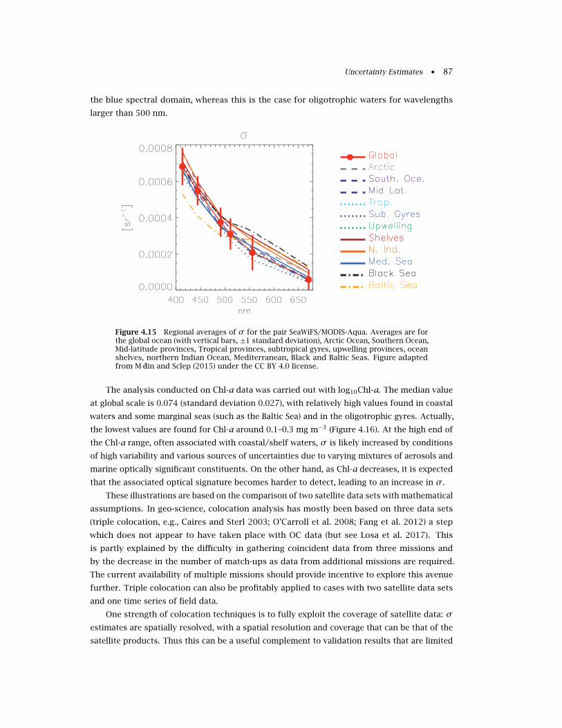
Uncertainty Estimates • 87
the blue spectral domain, whereas this is the case for oligotrophic waters for wavelengths
larger than 500 nm.
Figure 4.15 Regional averages of σ for the pair SeaWiFS/MODIS-Aqua. Averages are forthe global ocean (with vertical bars, ±1 standard deviation), Arctic Ocean, Southern Ocean,Mid-latitude provinces, Tropical provinces, subtropical gyres, upwelling provinces, oceanshelves, northern Indian Ocean, Mediterranean, Black and Baltic Seas. Figure adaptedfrom Mélin and Sclep (2015) under the CC BY 4.0 license.
The analysis conducted on Chl-a data was carried out with log10Chl-a. The median value
at global scale is 0.074 (standard deviation 0.027), with relatively high values found in coastal
waters and some marginal seas (such as the Baltic Sea) and in the oligotrophic gyres. Actually,
the lowest values are found for Chl-a around 0.1–0.3 mg m−3 (Figure 4.16). At the high end of
the Chl-a range, often associated with coastal/shelf waters, σ is likely increased by conditions
of high variability and various sources of uncertainties due to varying mixtures of aerosols and
marine optically significant constituents. On the other hand, as Chl-a decreases, it is expected
that the associated optical signature becomes harder to detect, leading to an increase in σ .
These illustrations are based on the comparison of two satellite data sets with mathematical
assumptions. In geo-science, colocation analysis has mostly been based on three data sets
(triple colocation, e.g., Caires and Sterl 2003; O’Carroll et al. 2008; Fang et al. 2012) a step
which does not appear to have taken place with OC data (but see Losa et al. 2017). This
is partly explained by the difficulty in gathering coincident data from three missions and
by the decrease in the number of match-ups as data from additional missions are required.
The current availability of multiple missions should provide incentive to explore this avenue
further. Triple colocation can also be profitably applied to cases with two satellite data sets
and one time series of field data.
One strength of colocation techniques is to fully exploit the coverage of satellite data: σestimates are spatially resolved, with a spatial resolution and coverage that can be that of the
satellite products. Thus this can be a useful complement to validation results that are limited
88 • Uncertainties in Ocean Colour Remote Sensing
Figure 4.16 Scatter plot of σ as a function of a multi-annual mean Chl-a. The line isconstructed from the median σ in each Chl-a bin of interval 0.05 in logarithmic units.
in terms of spatial and/or temporal distribution (e.g., Gregg and Casey 2004; Bailey and Werdell
2006). Conversely, the approach has a very limited capacity to provide temporally-resolved
information; in general the temporal discrimination that is attainable ultimately depends
on the number of matching pairs available for analysis (typically, seasonal estimates can be
derived when a multi-annual overlap period is considered).
4.2.14 Role of Biogeochemical Models
OC products have been used extensively as a source of validation for biogeochemical or
ecosystem model outputs. They have also been ingested into assimilation schemes to improve
model simulations at regional or global scales (e.g., Ford and Barciela 2017, Section 6.3). Some
assimilation experiments (Ciavatta et al. 2016) have made use of OC products such as Chl-a as
well as associated temporally and spatially resolved uncertainty fields (Jackson et al. 2017).
The converse set-up, whereby numerical models could support OC algorithms, has not been
much explored.
Different experiments have shown how different information sources, remote sensing and
otherwise, can be combined to help the interpretation of ecosystem conditions, particularly
in a three-dimensional context (Gould and Arnone 1998; Weisberg et al. 2004). Gould et al.
(2014) have run ensemble OC calculations (by varying TOA data) and ensemble hydrodynamical
simulations (transporting Chl-a fields) to gain insight into Chl-a product uncertainties. As far
as constraining the functioning of OC algorithms, the use of numerical models is largely an
untapped resource. Atmospheric circulation models can provide information on the type and
vertical structure of clouds and aerosols; even though numerical model outputs and satellite
imagery cannot be easily matched, the former might indicate the likelihood of conditions
Uncertainty Estimates • 89
where the algorithms applied to the latter are challenged (aerosol types not included in the
atmospheric correction, thin clouds etc.). A similar relationship is envisioned for the ocean.
Ecosystem models might detect if conditions are ripe for algal developments and thus provide
information about the probability of a bloom initiation; different approaches exist to model
and forecast blooms of harmful algae (HA) species (McGillicuddy 2010) often associated with
specific optical signatures, so that HA satellite products might be supported with this ancillary
information. Similarly, numerical models with a proper representation of rivers can give a
picture of the extent of a sediment plume in an estuary region. In such a case, if high Chl-a
values are found by OC processing, it is possible that they are largely erroneous. In general,
numerical model outputs could be used more extensively to assert the quality of the OC
products, or even to improve the processing.
Numerical models can also bring a strong added value to investigate how sampling can
affect level-3 satellite products. With increased spatial resolution, models can document finer
structures in biological fields (Lévy et al. 2012); further developments in that direction are
expected, with physical models tackling sub-kilometer scales (e.g., Jacobs et al. 2016), so that
heterogeneity within satellite pixels or grid points might be further investigated. As far as time
binning is concerned, numerical models are definitely a powerful tool to quantify the impact
of irregular sampling by satellite products. As discussed in Section 3.3, daily satellite data are
based on snapshots at certain times of the day (except for the case of geostationary platforms
that at least cover the daylight hours) while temporal (weekly, monthly) composites rely on a
limited number of days, a phenomenon that tends to increase the uncertainties associated with
level-3 data. Gregg and Casey (2007) investigated that issue by producing global time series of
Chl-a with a biogeochemical model (relying on satellite data assimilation) and sampling the
outputs as if observed by SeaWiFS or MODIS. The synthetic satellite time composites could
then be compared with composites based on the full model resolution. High latitudes were
particularly affected by the exclusion of satellite data processing for high solar zenith angles
and cloud cover. Recurrent cloud cover and high aerosol loads (like in the Arabian Sea in
summer or along the western African coasts) were responsible for large differences between
the two data sets, reaching tens of % in extreme cases. More such experiments are needed with
a view on providing realistic uncertainty estimates for level-3 satellite data.
The link between ocean colour and numerical models can be made more direct as some
numerical models include modules with a representation of optical properties providing the
ability to obtain as model outputs IOPs and RRS together with concentrations of optically
significant constituents such as Chl-a (e.g., Dutkiewicz et al. 2015; Baird et al. 2016). This
capability offers a whole range of opportunities for testing and understanding OC products and
model outputs. For instance, Dutkiewicz et al. (2018) compared Chl-a derived from satellite
with Chl-a obtained as direct output of a numerical model as well as Chl-a computed from
the model derived RRS with standard OC algorithms, the latter being closest to the satellite
product. An interesting result is the possible mismatch in annual cycle seen between Chl-a as
direct output of the biology model and Chl-a computed from the model RRS with a band-ratio
algorithm, which provides some potential insight on modeling issues or on how satellite Chl-a
might be affected by varying uncertainties during the annual cycle.
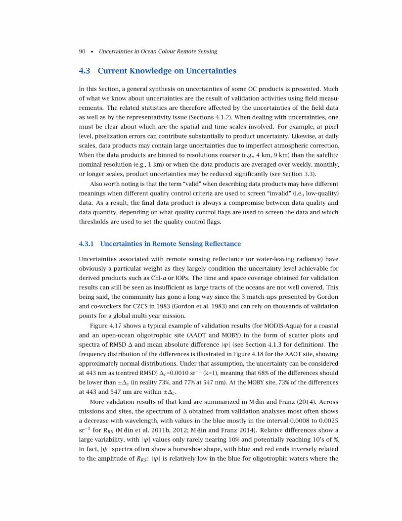
90 • Uncertainties in Ocean Colour Remote Sensing
4.3 Current Knowledge on Uncertainties
In this Section, a general synthesis on uncertainties of some OC products is presented. Much
of what we know about uncertainties are the result of validation activities using field measu-
rements. The related statistics are therefore affected by the uncertainties of the field data
as well as by the representativity issue (Sections 4.1.2). When dealing with uncertainties, one
must be clear about which are the spatial and time scales involved. For example, at pixel
level, pixelization errors can contribute substantially to product uncertainty. Likewise, at daily
scales, data products may contain large uncertainties due to imperfect atmospheric correction.
When the data products are binned to resolutions coarser (e.g., 4 km, 9 km) than the satellite
nominal resolution (e.g., 1 km) or when the data products are averaged over weekly, monthly,
or longer scales, product uncertainties may be reduced significantly (see Section 3.3).
Also worth noting is that the term “valid” when describing data products may have different
meanings when different quality control criteria are used to screen “invalid” (i.e., low-quality)
data. As a result, the final data product is always a compromise between data quality and
data quantity, depending on what quality control flags are used to screen the data and which
thresholds are used to set the quality control flags.
4.3.1 Uncertainties in Remote Sensing Reflectance
Uncertainties associated with remote sensing reflectance (or water-leaving radiance) have
obviously a particular weight as they largely condition the uncertainty level achievable for
derived products such as Chl-a or IOPs. The time and space coverage obtained for validation
results can still be seen as insufficient as large tracts of the oceans are not well covered. This
being said, the community has gone a long way since the 3 match-ups presented by Gordon
and co-workers for CZCS in 1983 (Gordon et al. 1983) and can rely on thousands of validation
points for a global multi-year mission.
Figure 4.17 shows a typical example of validation results (for MODIS-Aqua) for a coastal
and an open-ocean oligotrophic site (AAOT and MOBY) in the form of scatter plots and
spectra of RMSD ∆ and mean absolute difference |ψ| (see Section 4.1.3 for definition). The
frequency distribution of the differences is illustrated in Figure 4.18 for the AAOT site, showing
approximately normal distributions. Under that assumption, the uncertainty can be considered
at 443 nm as (centred RMSD) ∆c=0.0010 sr−1 (k=1), meaning that 68% of the differences should
be lower than ±∆c (in reality 73%, and 77% at 547 nm). At the MOBY site, 73% of the differences
at 443 and 547 nm are within ±∆c .More validation results of that kind are summarized in Mélin and Franz (2014). Across
missions and sites, the spectrum of ∆ obtained from validation analyses most often shows
a decrease with wavelength, with values in the blue mostly in the interval 0.0008 to 0.0025
sr−1 for RRS (Mélin et al. 2011b, 2012; Mélin and Franz 2014). Relative differences show a
large variability, with |ψ| values only rarely nearing 10% and potentially reaching 10’s of %.
In fact, |ψ| spectra often show a horseshoe shape, with blue and red ends inversely related
to the amplitude of RRS : |ψ| is relatively low in the blue for oligotrophic waters where the
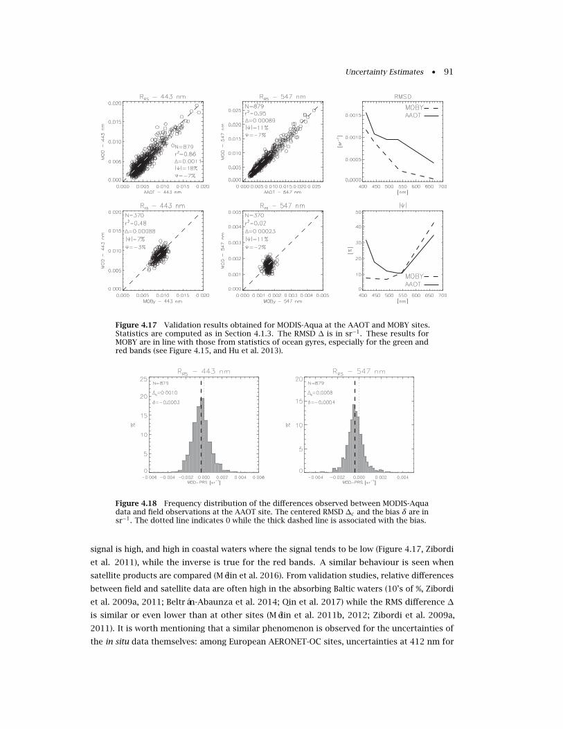
Uncertainty Estimates • 91
Figure 4.17 Validation results obtained for MODIS-Aqua at the AAOT and MOBY sites.Statistics are computed as in Section 4.1.3. The RMSD ∆ is in sr−1. These results forMOBY are in line with those from statistics of ocean gyres, especially for the green andred bands (see Figure 4.15, and Hu et al. 2013).
Figure 4.18 Frequency distribution of the differences observed between MODIS-Aquadata and field observations at the AAOT site. The centered RMSD ∆c and the bias δ are insr−1. The dotted line indicates 0 while the thick dashed line is associated with the bias.
signal is high, and high in coastal waters where the signal tends to be low (Figure 4.17, Zibordi
et al. 2011), while the inverse is true for the red bands. A similar behaviour is seen when
satellite products are compared (Mélin et al. 2016). From validation studies, relative differences
between field and satellite data are often high in the absorbing Baltic waters (10’s of %, Zibordi
et al. 2009a, 2011; Beltrán-Abaunza et al. 2014; Qin et al. 2017) while the RMS difference ∆is similar or even lower than at other sites (Mélin et al. 2011b, 2012; Zibordi et al. 2009a,
2011). It is worth mentioning that a similar phenomenon is observed for the uncertainties of
the in situ data themselves: among European AERONET-OC sites, uncertainties at 412 nm for
92 • Uncertainties in Ocean Colour Remote Sensing
RRS are lowest at the Baltic sites when expressed in radiometric units but highest (15-25%)
when expressed in relative terms (Gergely and Zibordi 2014). Results so far obtained from
spatially-resolved techniques (Section 4.2) need further analysis. First conclusions from the
clear-water and colocation approaches (Sections 4.2.4 and 4.2.13, respectively) suggest that
standard SeaWiFS and MODIS products fulfill a 5% uncertainty only at blue wavelengths and
for oligotrophic waters (Hu et al. 2013; Mélin et al. 2016).
Uncertainty statistics for RRS would need to be further analysed and understood but a
certain number of results have already appeared. For a given site, differences between field
and satellite data appear well correlated, and are therefore not randomly distributed, across
the spectrum. For instance, the correlation coefficient r between differences for the bands 412,
443 and 488 nm is larger than 0.8 for both sites of Figure 4.17 (AAOT and MOBY). At AAOT,
differences at 443 nm are correlated with those at 547 and 667 nm with r equal to 0.72 and
0.64, respectively; these numbers are 0.86 and 0.53 at MOBY (this suggests that part of the
errors affecting RRS do not affect band-ratio algorithms). These results are in line with those
obtained from the clear water approach described in Section 4.2.4 (Hu et al. 2013).
The discussion above suggests that validation results might depend on the water type,
which has been confirmed by studies applying optical classification techniques to characterize
the differences between satellite and field data (Goyens et al. 2013; Mélin and Franz 2014;
Moore et al. 2015), and applied to derive spatially-resolved uncertainty estimates (Jackson et al.
2017, Section 4.2.5). D’Alimonte et al. (2008) have even presented a regional multi-linear model
to predict the difference between field and satellite values as a function of the spectrum of RRS .
How these differences evolve with respect to quantities such as geometry (solar or viewing
zenith angles), aerosol load or type, water single-scattering-albedo, chlorophyll concentration,
distance to the coast, have been investigated (Schollaert et al. 2003; Mélin et al. 2007a; Zibordi
et al. 2012a; Kajiyama et al. 2014; Barnes and Hu 2016; Bulgarelli et al. 2017), but conclusions
are hard to reach as it appears difficult to disentangle the various dependences; the use of
modeled cases might be more efficient in that regard (IOCCG 2010). Some effects can be
mission-dependent, for instance, in terms of cross-track variations (Mueller et al. 2015b).
4.3.2 Derived Products
Once the atmospheric contribution is dealt with, estimates of derived in-water products can be
computed. In association with its varied applications (IOCCG 2008), ocean colour now has a
long list of derived products (chlorophyll concentration, spectral inherent optical properties,
diffuse attenuation coefficient Kd, particulate/dissolved organic carbon, particulate inorganic
carbon, Secchi depth, euphotic depth, phytoplankton functional types and size classes etc.) so
that a complete discussion of the current knowledge associated with each exceeds the capacity
of this report, all the more so that it is a fast evolving subject for the most recent products.
In general, uncertainties of derived products are expected to increase as processing layers
are added (Figure 3.3). In a remote sensing context, the uncertainties of these products are
affected by the uncertainties of the algorithm inputs, the satellite RRS , while algorithms have
often been tested using field data of RRS , knowing that the resulting uncertainty values are
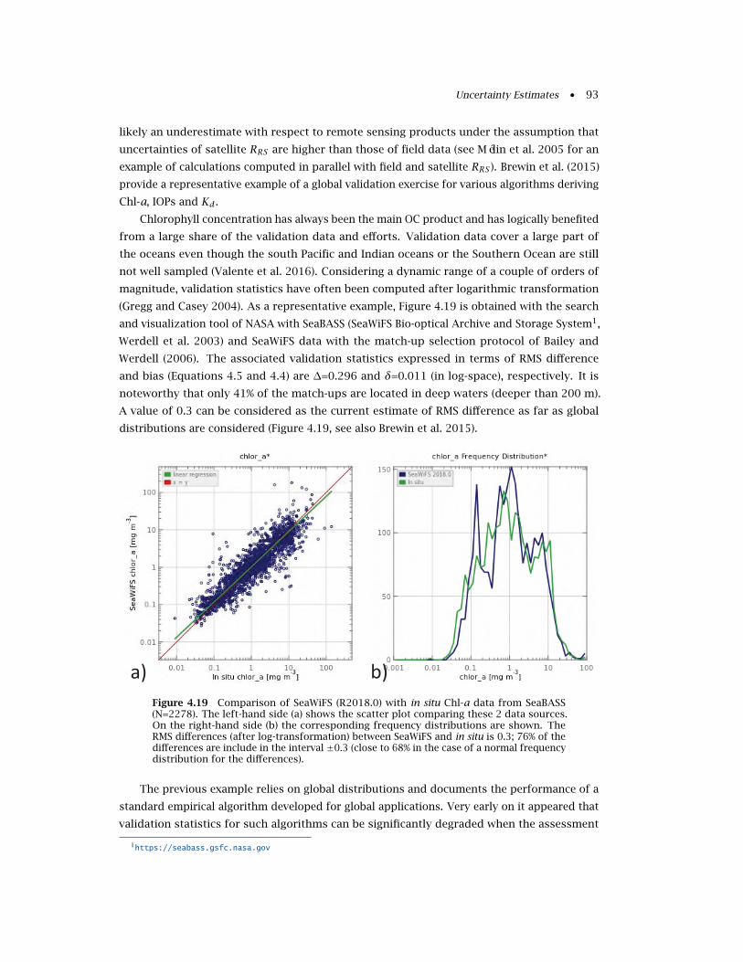
Uncertainty Estimates • 93
likely an underestimate with respect to remote sensing products under the assumption that
uncertainties of satellite RRS are higher than those of field data (see Mélin et al. 2005 for an
example of calculations computed in parallel with field and satellite RRS ). Brewin et al. (2015)
provide a representative example of a global validation exercise for various algorithms deriving
Chl-a, IOPs and Kd.
Chlorophyll concentration has always been the main OC product and has logically benefited
from a large share of the validation data and efforts. Validation data cover a large part of
the oceans even though the south Pacific and Indian oceans or the Southern Ocean are still
not well sampled (Valente et al. 2016). Considering a dynamic range of a couple of orders of
magnitude, validation statistics have often been computed after logarithmic transformation
(Gregg and Casey 2004). As a representative example, Figure 4.19 is obtained with the search
and visualization tool of NASA with SeaBASS (SeaWiFS Bio-optical Archive and Storage System1,
Werdell et al. 2003) and SeaWiFS data with the match-up selection protocol of Bailey and
Werdell (2006). The associated validation statistics expressed in terms of RMS difference
and bias (Equations 4.5 and 4.4) are ∆=0.296 and δ=0.011 (in log-space), respectively. It is
noteworthy that only 41% of the match-ups are located in deep waters (deeper than 200 m).
A value of 0.3 can be considered as the current estimate of RMS difference as far as global
distributions are considered (Figure 4.19, see also Brewin et al. 2015).
a) b)Figure 4.19 Comparison of SeaWiFS (R2018.0) with in situ Chl-a data from SeaBASS(N=2278). The left-hand side (a) shows the scatter plot comparing these 2 data sources.On the right-hand side (b) the corresponding frequency distributions are shown. TheRMS differences (after log-transformation) between SeaWiFS and in situ is 0.3; 76% of thedifferences are include in the interval ±0.3 (close to 68% in the case of a normal frequencydistribution for the differences).
The previous example relies on global distributions and documents the performance of a
standard empirical algorithm developed for global applications. Very early on it appeared that
validation statistics for such algorithms can be significantly degraded when the assessment
1https://seabass.gsfc.nasa.gov
94 • Uncertainties in Ocean Colour Remote Sensing
is performed at a regional scale and/or a specific season. It is now well established that the
performance associated with Chl-a algorithms shows strong regional variations (Dierssen
2010; Szeto et al. 2011), as specific IOPs of phytoplankton as well as the relative importance
of other optically significant constituents vary, as discussed in Section 3.2.4. Specific cases
observed in marginal seas, coastal waters, Arctic or Southern Oceans are well documented (e.g.,
Dierssen and Smith 2000; Cota et al. 2004; Volpe et al. 2007; Johnson et al. 2013), leading to
the development of many regional algorithms or the application of semi-analytical bio-optical
models thought to be more generic (even though their parameters may also be appropriate
only for specific regions). It is in general expected that Chl-a relative uncertainties tend to be
higher in low-Chl-a oligotrophic waters, in relation to sensitivity issues, and in coastal regions,
where the influence of other constituents is increasingly felt, as confirmed by colocation results
(Mélin 2010, Section 4.2.13).
The quantity of match-ups or, in general, of assessment results decreases for variables like
Kd, absorption IOPs and backscattering coefficients. The results of Brewin et al. (2015) indicates
a RMS difference between log-transformed in situ data and algorithm outputs of approximately
0.2 at 412 nm and 0.15 at 490 nm for the total absorption coefficient. These differences tend
to increase when total absorption is partitioned into separate components for phytoplankton
or detrital material. It should be remembered that these estimates of uncertainties could be
still higher for remote sensing data; conversely, they also include components associated with
the issue of representativeness and the uncertainties associated with in situ data.
4.3.3 Phytoplankton Groups
Since the turn of the century, there has been an increasing interest in retrieving information
on the community composition of phytoplankton from satellite measurements of ocean
colour. This research has been driven from the realisation that better understanding of
global cycles of major elements in the ocean (e.g., carbon and nitrogen) requires an improved
representation of the community composition of phytoplankton at synoptic scales. Many
approaches have been presented that target single or multiple phytoplankton groups, some
focused on retrieving dominance, others on the concentrations in chlorophyll or in carbon
units. In general, approaches can be separated into detection-based methods that target
distinct optical signatures of the phytoplankton groups, or extrapolation-based methods that
relate the phytoplankton groups to some variable(s) that can be retrieved with confidence from
space, either directly from ocean colour (e.g., chlorophyll, abundance-based) or in combination
with other ocean satellite products (e.g., sea surface temperature, ecologically-based). IOCCG
(2014) provide a state-of-the-art review of all these techniques and discuss their advantages
and limitations (see also Mouw et al. 2017).
Whereas a wide variety of techniques have been developed, like with many OC products,
uncertainties are rarely provided. In cases where they have been quantified, either error
propagation (model-based) methods have been used (e.g., Kostadinov et al. 2009, 2016; Roy
et al. 2013; Brewin et al. 2017a), or uncertainties have been estimated through comparison of
satellite estimates with in situ data (see Table 4 of Mouw et al. 2017), including approaches that
Uncertainty Estimates • 95
use optical water types or provinces for mapping errors (Brewin et al. 2017b; Losa et al. 2017).
There have also been attempts to use triple collocation analysis of satellite and ecosystem
model data for quantifying uncertainties in phytoplankton groups (Losa et al. 2017).
Estimates of uncertainty through error propagation requires good knowledge of the
uncertainties in the inputs and the parameters of the model, which will depend on the datasets
used to train the model and the range of conditions for which the method was developed. For
detection-based methods, the optical signatures of the phytoplankton groups being targeted
can be small and hard to detect (Garver et al. 1994; Wang et al. 2005), meaning uncertainties will
vary depending on optical environment. In cases where phytoplankton co-vary predictably with
other optically-significant substances (e.g., Case 1 conditions), it can be difficult to determine
whether a change in the reflectance spectrum has been caused by a change in the phytoplankton
community composition or by a change in the chlorophyll concentration (Sathyendranath et al.
2017). All these factors make it challenging to derive model-based estimates of uncertainty. It
is expected that by increasing the spectral resolution of satellite sensors, methods for deriving
phytoplankton groups and model-based uncertainties will improve.
As discussed previously in this report, uncertainties estimated through comparison of
satellite and in situ data typically consider the in situ data to be the truth, when in reality
field data have their own uncertainties (not mentioning the difference in scales discussed
previously). This is particularly true for phytoplankton community structure, considering
there is no standard technique used to measure phytoplankton community structure in situ,
and though different methods have been compared (e.g., Brewin et al. 2014), uncertainties
in field data on phytoplankton groups are not known well (Nair et al. 2008). The difficulty
with developing a standard in situ technique is that approaches have been developed to detect
different phytoplankton groups depending on the scientific question being addressed, using
different metrics of detection (chlorophyll, carbon, cell counts), and with different objectives
(e.g., targeting dominance or concentration). This makes it challenging to inter-compare
approaches (Brewin et al. 2011; Losa et al. 2017) and to derive estimates of uncertainty through
comparison with in situ data. Certainly more work is needed in that regard (Bracher et al.
2017).
4.3.4 Aerosol Products
Through the process of atmospheric correction, OC data may include aerosol products, typically
aerosol optical thickness τa and Ångström exponent α. Strictly speaking the validation of these
products is interesting only insofar as they are quantitatively used for a specific application.
If the aerosol component is explicitly modelled in the atmospheric correction, the quantity
that matters is the impact of the aerosol on the atmospheric path radiance. This being said,
it is legitimate to consider that poor results in terms of τa and/or α suggest an inadequate
functioning of the AC algorithm.
The emergence of measurement networks of Sun photometers has provided a large body
of data suitable for validation. It has been shown that sites from AERONET (Holben et al.
1998) located on small islands or capes can be used for validation of OC data with appropriate
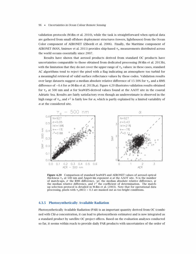
96 • Uncertainties in Ocean Colour Remote Sensing
validation protocols (Mélin et al. 2010), while the task is straightforward when optical data
are gathered from small offshore deployment structures (towers, lighthouses) from the Ocean
Color component of AERONET (Zibordi et al. 2006). Finally, the Maritime component of
AERONET (MAN, Smirnov et al. 2011) provides ship-based τa measurements distributed across
the world oceans essentially since 2007.
Results have shown that aerosol products derived from standard OC products have
uncertainties comparable to those obtained from dedicated processing (Mélin et al. 2013b),
with the limitation that they do not cover the upper range of τa values: in these cases, standard
AC algorithms tend to reject the pixel with a flag indicating an atmosphere too turbid for
a meaningful retrieval of valid surface reflectance values by these codes. Validation results
over large datasets suggest a median absolute relative difference of 15-30% for τa and a RMS
difference of ∼0.4 for α (Mélin et al. 2013b,a). Figure 4.20 illustrates validation results obtained
for τa at 500 nm and α for SeaWiFS-derived values found at the AAOT site in the coastal
Adriatic Sea. Results are fairly satisfactory even though an underestimate is observed in the
high range of τa, and r 2 is fairly low for α, which is partly explained by a limited variability of
α at the considered site.
Figure 4.20 Comparison of standard SeaWiFS and AERONET values of aerosol opticalthickness τa at 500 nm and Ångström exponent α at the AAOT site. N is the numberof match-ups, σ the RMS difference, |ψ| the median absolute relative difference, ψthe median relative difference, and r 2 the coefficient of determination. The match-up selection protocol is detailed in Mélin et al. (2003). Note that for operational dataprocessing, pixels with τa(865) > 0.3 are masked out as too bright conditions.
4.3.5 Photosynthetically Available Radiation
Photosynthetically Available Radiation (PAR) is an important quantity derived from OC (combi-
ned with Chl-a concentration, it can lead to photosynthesis estimates) and is now integrated as
a standard product by satellite OC project offices. Based on the evaluation analyses conducted
so far, it seems within reach to provide daily PAR products with uncertainties of the order of
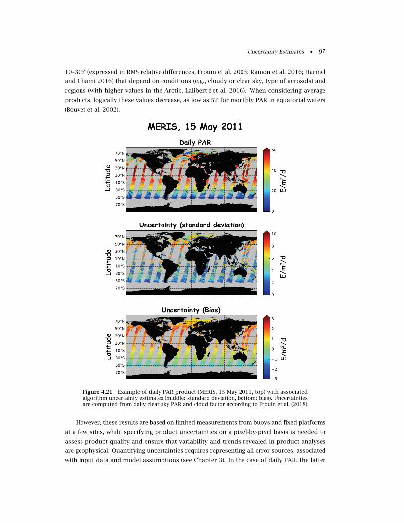
Uncertainty Estimates • 97
10–30% (expressed in RMS relative differences, Frouin et al. 2003; Ramon et al. 2016; Harmel
and Chami 2016) that depend on conditions (e.g., cloudy or clear sky, type of aerosols) and
regions (with higher values in the Arctic, Laliberté et al. 2016). When considering average
products, logically these values decrease, as low as 5% for monthly PAR in equatorial waters
(Bouvet et al. 2002).
Figure 4.21 Example of daily PAR product (MERIS, 15 May 2011, top) with associatedalgorithm uncertainty estimates (middle: standard deviation, bottom: bias). Uncertaintiesare computed from daily clear sky PAR and cloud factor according to Frouin et al. (2018).
However, these results are based on limited measurements from buoys and fixed platforms
at a few sites, while specifying product uncertainties on a pixel-by-pixel basis is needed to
assess product quality and ensure that variability and trends revealed in product analyses
are geophysical. Quantifying uncertainties requires representing all error sources, associated
with input data and model assumptions (see Chapter 3). In the case of daily PAR, the latter
98 • Uncertainties in Ocean Colour Remote Sensing
include elements such as decoupling effects of clouds and clear atmosphere, neglecting diurnal
variability of clouds, or the use of an aerosol climatology. Assuming that the input variables
(TOA reflectance at wavelengths in the PAR spectral range) have little impact on the total
uncertainty budget, a procedure to estimate the uncertainty for each pixel of a product is
described in Frouin et al. (2018). The bias and standard deviation of the daily PAR estimates
are calculated as a function of clear sky PAR and cloud factor (that characterizes the effect of
clouds on daily PAR and varies from 0 to 1) by simulating for a wide range of situations the
satellite measurements and the corresponding daily PAR values.
Figure 4.21 displays an example of global MERIS daily PAR product and associated un-
certainties, expressed as standard deviation and bias. The uncertainty characterization was
done using an extensive simulation dataset covering 2003–2012 with hourly Modern-Era Re-
trospective analysis for Research and Applications version 2 (MERRA-2) data as input. Using
MERRA-2 products, atmospheric variability, in particular diurnal cloudiness, is well sampled
at all latitudes. Standard deviation and bias range approximately from 1 to 8 E m−2 d−1 and
-1 to +2 E m−2 d−1 respectively, with larger values corresponding to higher clear sky PAR
and intermediate (i.e., 0.4–0.8) cloud factor. A complete per-pixel uncertainty budget would
include uncertainties associated with measurement noise and radiometric calibration, which
may require estimating the sensitivity of daily PAR to input reflectance and covariance in the
various spectral bands. Note, however, that comparisons with match-up data at the Chesapeake
Bay CERES Ocean Validation Experiment site, not shown here, have revealed that experimental
uncertainties are similar to the theoretical algorithm uncertainties obtained from simulated
data.
4.3.6 Primary Production
Primary production is not a standard OC product because it needs further elaboration from
quantities such as Chl-a, IOPs and PAR, but it has appeared early on as one of the major
variables that can be obtained from ocean colour (e.g., Platt and Sathyendranath 1988) and it is
interesting to understand how uncertainties on the various OC products are propagated when
they are combined into a higher-level quantity. The structure of primary production models
has taken different levels of complexity, from vertically- and spectrally-integrated empirical
algorithms to vertically- and spectrally-resolved models (Behrenfeld and Falkowski 1997); while
theoretical studies have evaluated the impact of specific simplifying assumptions (for instance
on the spectral character of light or the vertical structure of biomass, Sathyendranath et al.
1989; Kyewalyanga et al. 1992), here the issue of the associated uncertainties can only briefly
be touched upon.
Approximately, primary productivity is a function of biomass that can be represented by
Chl-a (Platt and Sathyendranath 1988), irradiance and photosynthetic parameters, leading Platt
et al. (1988) to propose a lower bound of uncertainties of 42% considering an uncertainty of
35% and 10% for satellite products of Chl-a and irradiance and assuming an uncertainty of 20%
for the biomass-normalized initial slope of the light-photosynthesis curve determined in the
field (and 5% for its assimilation number). Further considering that values of photosynthetic
Uncertainty Estimates • 99
parameters may vary within a given biogeochemical ocean province, Platt et al. (1995) gave
an uncertainty of 50% for satellite-derived primary production estimates, the uncertainty on
Chl-a being the dominant factor. This is actually comparable to the RMS difference of 0.3
in log10-units (equivalent to a factor ∼2) typically obtained for some models participating in
Primary Production Algorithm Round-Robin (PPARR) exercises in widely distributed regions
(Friedrichs et al. 2009; Saba et al. 2010, 2011), while some models or specific areas may show
either larger values (like the Arctic Ocean, Lee et al. 2015a) or better results (Silsbe et al.
2016). However, it is stressed that these evaluation exercises are different. While the estimate
proposed by Platt et al. (1988) assumes that the bio-optical conditions (IOPs, vertical structure
etc.) and the photosynthetic parameters are reasonably well known, the PPARR exercises
usually provide Chl-a values measured in the field (presumably with an uncertainty lower than
that of the satellite value) as model inputs.
4.4 Verification of Uncertainties
Uncertainty estimates attached to remote sensing products in turn need to be verified. In the
field of ocean colour remote sensing, this step is certainly in its infancy. A couple of points
can however be made.
At least for the main OC products, a consistent picture of uncertainty estimates as
obtained by comparison with field data, has emerged (Section 4.3). Certainly, match-ups are
not necessarily evenly distributed in space and time, which is a limitation when it comes to
interpreting validation statistics at the scale of a mission, but there are enough elements to
draw some general conclusions about the magnitudes of differences and their behavior as a
function of wavelength or specific conditions (geometry, water types), locations and seasons.
Most of the methods introduced in Section 4.2 do not make use of field data in a direct
manner (with the exception of the approaches based on optical water types), which has the
advantage of preserving matchup data sets as an independent source of verification, even
though as yet this potential has been insufficiently exploited. Maritorena et al. (2010) compared
validation statistics with estimates obtained from a non-linear least-square inversion applied to
a bio-optical model (see Section 4.2.6). Mélin et al. (2016) confronted validation results for RRSwith outputs from a co-location approach (Section 4.2.13) and an optical-type approach (Section
4.2.5, Jackson et al. 2017) at four sites equipped with autonomous systems, and concluded
to a reasonable agreement (with some exceptions). Ultimately, uncertainty estimates need to
be confronted with validation statistics but this comparison needs to be conducted between
equivalent quantities (i.e., considering the same sources of uncertainty in their budget), which
is not straightforward as the different approaches are based on different hypotheses and
mathematical frameworks (see discussion below). It is clear that validation statistics will play
a key role in the verification of uncertainty estimates but this role will be fulfilled only if i) the
uncertainties associated with the field data are known, and ii) the issue of representativeness
(including potential definitional discrepancies, see Section 4.1.2) is properly taken into account.
The fact that most of the approaches described in Section 4.2 are fairly recent and often
100 • Uncertainties in Ocean Colour Remote Sensing
not included in operational processing partly explains why their outputs mostly have not
been compared. Mélin et al. (2016) compared results from a co-location experiment with
outputs from the clear-water approach (Section 4.2.4, Hu et al. 2013) and an optically-based
approach (Section 4.2.5, Jackson et al. 2017), and the studies of Hu et al. (2013) and Mélin
et al. (2016) concurred to suggest that the SeaWiFS and MODIS data fulfilled the objective of a
5% uncertainty for RRS in the blue in oligotrophic waters. For these two studies uncertainty
estimates for RRS at 443 nm and 555 nm are of the order of approximately 4–5 × 10⁻⁴ sr−1
and 2 × 10⁻⁴ sr−1, respectively (compare Figures 4.2 and 4.15). Results obtained by a Monte
Carlo approach (Section 4.2.9) show significantly lower values (approximately by a factor 2,
see Figure 4.9). But as anticipated above, these techniques are not operating in the same
theoretical framework. The comparison of results obtained from different techniques needs
to be underpinned by a solid understanding of how each method is constructed, particularly
regarding the hypotheses underlying the methods, the considered sources of uncertainty (and
those ignored), and the nature of the uncertainty estimates. A first brief discussion is provided
here.
First some methods have inherent limitations in space or time. The co-location approach
is spatially resolved but is extremely limited in terms of temporal resolution, while the
clear-water approach has a telling name. In their own way, both methods encompass all
sources of uncertainties bearing on RRS (associated with top-of-atmosphere calibration and
atmospheric correction) but without considering systematic contributions. Actually, systematic
contributions to the uncertainty budget are not covered in most cases introduced in Section
4.2. Techniques relying on the outputs of non-linear least-square inversions do not include
structural uncertainty, and their uncertainty estimate has more to do with the fitting quality
of the inversion. Approaches based on uncertainty propagation, either through Monte-Carlo
simulations or Taylor expansions, are very versatile in their ability to represent all sources
of uncertainties (with the exception of systematic contributions in the latter case), but so
far a selection has been made to circumvent the complexity of the problem. When applied
to atmospheric correction, there has been a focus on the uncertainties associated with the
TOA signal (Neukermans et al. 2009; OLCI 2013; Franz and Karaköylü 2016). In the case of
bio-optical algorithms, the uncertainties associated with algorithm parameters and with the
input RRS have rarely been considered together.
Among the various methods illustrated in Section 4.2, those based on optical water types
have the peculiarity of being based on field observations and matchup data sets. Their
operation is actually a way to extend validation statistics (including bias estimates) at larger
scales (Moore et al. 2009; Jackson et al. 2017). They are based on the hypothesis that water
types can be a significant predictor of uncertainty estimates. Having used validation data
for its construction, they are more limited to find independent validation data to assess the
method outputs. While their outputs seem familiar with respect to the well-practiced validation
statistics, they do not represent the uncertainties of the satellite data since the uncertainties
associated with in situ data and the issue of representativeness are not excluded (albeit these
aspects could be considered in future developments). One advantage of this approach is that
its outputs are obviously related to field data and therefore potentially traceable to reference

Uncertainty Estimates • 101
standards more readily available than those associated with a sensor in space.
The diversity of methods producing uncertainty estimates in the field of ocean colour
offers an interesting potential when it comes to covering all aspects of this multi-faceted
problem and ultimately obtaining a full uncertainty budget but certainly a lot more work is
needed to produce and verify uncertainty estimates in a mature way.

102 • Uncertainties in Ocean Colour Remote Sensing
Chapter 5
Representation and Distribution of Uncertainties
Frédéric Mélin, Nicolas Lamquin, Thomas Jackson, Stéphane Maritorena and
Gianluca Volpe
This chapter discusses some issues relevant for the representation and distribution of flag
values and uncertainty estimates, and introduces some data streams that include uncertainty
estimates in their products.
5.1 Flags
Remote sensing products are traditionally accompanied by (quality) flag values1; they represent
additional information to the data documenting how the processing led to the reported data
value. In case the data value is considered not valid (usually marked with a specific code
termed “bad” value), the pixel is masked and the flag typically indicates the reason why the
processing was interrupted (e.g., land; observed radiance beyond what is considered a valid
range, contaminated by stray light or saturated; absence of ancillary or navigation data; failure
of the algorithm). As indicated in Section 4.2.1, some flags are related to the functioning of the
sensor, some are based on specific algorithms independent from the main processing (e.g., the
detection of clouds or glint conditions), while some are directly associated with the functioning
of the retrieval algorithm (e.g., absence of convergence of an algorithm). Other communities
have organized their flagging system through a scale of increasing quality where each level is
associated with specific applications and requirements (Kilpatrick et al. 2001).
The availability of flags is useful to advise users as to the quality of the product and
the applicability of a datum for a particular purpose. As uncertainty distributions become
systematically available for remote sensing products, the question of the connections between
flag values and uncertainty estimates is raised. To some extent, an uncertainty estimate
associated with each datum might render some information brought by flags irrelevant.
However, even with uncertainty estimates, flag arrays will keep most of their merit. First of
all, they inform the user on the reason for a failed processing. Then, even when a retrieval
is given, it is important to make a clear distinction between quality (as suggested by flag
values) and uncertainty (Merchant et al. 2017): a product can be considered of a high quality
regardless of the magnitude of its uncertainty, meaning that the user can have confidence in
1examples in https://oceancolor.gsfc.nasa.gov/atbd/ocl2flags/
103
104 • Uncertainties in Ocean Colour Remote Sensing
the product value within the stated uncertainty (in other words, high uncertainty does not
necessarily mean low quality of the retrieval). On the other hand, out-of-scope conditions
might be detected and coded by flags, suggesting caution or even exclusion of a pixel, again
regardless of the magnitude of the uncertainty. However, there is still a relationship between
uncertainty and flags when flags have a bearing on the domain of applicability of algorithms.
Below are simplified categories of flags (as anticipated above) and how they relate to uncertainty
distribution. Across these categories, flags are of two principal natures, depending on whether
they trigger an invalid value for the product (discarded data). In that case of exclusive flags,
they are expected to explain why the processing did not proceed. If a product is found, a flag
array provides quality indicators or warning notes merely suggesting caution in the use of the
data.
i) The first category of flags records conditions related to the functioning of the sensor
and that are to some extent independent of the scientific algorithms being applied. They
record instances of sensor anomalies, sensor saturation, or the absence of ancillary or
navigation data. Flags can also document the application of the calibration equation that
should produce the spectrum of TOA radiance together with its uncertainty. Flag values
can register cases of observed radiance beyond what is considered a valid range or any
other warning about the calibration process.
ii) Somewhat artificially, we may consider flags associated with specific algorithms or tests
independent of the scientific algorithms (atmospheric correction, bio-optical in-water al-
gorithms). These tests might document conditions of the surface (detection of land or
clouds, cloud shadow, high fraction of white caps, glint conditions etc.) or extreme geo-
metry (high viewing or solar zenith angles). Some of the related conditions hamper any
OC retrieval (presence of land, cloud or high glint for many algorithms) while others only
provide warning messages. Tests are often based on threshold values (on TOA radiance,
angles, wind speed etc.) that have a direct impact on the spatial coverage of the product. If
thresholds are released, the coverage will expand but the uncertainty is likely to increase, a
behavior that should be reflected in the scheme providing the uncertainty estimates. By
the same token, if the process of computing uncertainties has made assumptions on these
thresholds, it might have to be revised if more challenging conditions (lower Sun, higher
wind speed) are allowed in the data processing. For the sake of completeness, it is worth
reminding that ancillary data entering into flagging tests are also characterized by their
own uncertainties (see Section 3.1.2).
iii) Then, other flags are more directly associated with the functioning of the scientific algo-
rithms (atmospheric correction, bio-optical in-water algorithms). They may indicate a failure
of the algorithm (e.g., lack of convergence), or outputs that suggest caution in the interpre-
tation of results (e.g., aerosol type or optical thickness out of the bounds expected for the
algorithm, suspiciously low water-leaving radiance). It is possible that an advanced method
to derive uncertainties might, in these conditions, produce valid (and likely relatively high)
estimates. But as indicated above, it is also possible that both the scientific algorithm and
the method to derive uncertainties be out of their conditions of applicability, in which case
Representation and Distribution of Uncertainties • 105
the uncertainty estimate is as suspicious as the algorithm output.
The flag arrays accompanying the OC products are an important component of the data
streams, the use of which could actually be extended. Whatever the amount of information
that is conveyed by flags, algorithms, uncertainty calculations and flagging systems need to be
fully integrated in a coherent ensemble, both in the development stage and in the distributed
data stream.
5.2 Uncertainty Distribution
Ideally an uncertainty estimate for each datum should inform the user on “the dispersion of the
values that could reasonably be attributed to the measurand” (GUM 2008). Such information
can be conveyed through various means, from providing a complete probability distribution
function (PDF) to giving percentiles, a confidence interval or even a single value (like a multiple
of a standard deviation with its coverage factor, see Chapter 2). In turn, the interpretation
of a single number in terms of PDF relies on assumptions on the properties of the PDF itself
(typically a hypothesis of normality) that should be verified. Discrete quantities might require
specific description of their uncertainties, for instance misclassification rates (Section 4.1.3).
Providing uncertainty estimates in absolute terms (in the same units as the data) or in relative
terms (in %) is equivalent for the pixel-based satellite level-1 and level-2 data (as the conversion
from one to the other is straightforward). This is no longer true when going to level-3 sets that
imply an aggregation of data. For uncertainty propagation through that process, it might be
preferable to express uncertainties in absolute terms as uncertainties are written as standard
deviations (see Section 3.3). Quantifying uncertainties in absolute terms might also be more
convenient when measurands are very low within their range of variability. OC variables
are often associated with a hypothesis of log-normality (Campbell 1995), and consequently
uncertainties have been expressed for log-transformed data, which can be directly related
to uncertainties expressed in relative terms (the difference of logarithms being equal to the
logarithm of the ratio of the two arguments). As explained in the previous Section (5.1), the
flagging set might be revised or completed in relation to the uncertainty fields but it conveys a
different type of (complementary) information, including an indication whether the data value
and its uncertainty are indeed valid.
Additional information about the spatial and temporal structure of the uncertainties
(covariance matrices, length scales) is needed to make full use of their values. Assuming
that the information is available, including a full description of the uncertainty field for each
distributed datum is not practicable because of storage issues, and ways to summarize its
major properties will need to be found (Merchant et al. 2019). It is acknowledged that the
presentation of uncertainties might vary as a function of the variable or application conside-
red. For some users, a single value representing total uncertainty might be sufficient, while
covariance information might be required for other applications, such as data assimilation
(Ford and Barciela 2017). In general, the presentation of uncertainty information faces con-
flicting requirements, of maintaining reasonable data volumes and ease of use by the user
106 • Uncertainties in Ocean Colour Remote Sensing
community while providing complete information about the uncertainty budget, allowing its
propagation through temporal/spatial averages and permitting a control over its long-term
stability (Merchant et al. 2017).
The next Section provides a description of uncertainty fields currently available to the
community.
5.3 Current Distributions
Some methods described in Section 4.2 have been applied to large-scale data sets with uncer-
tainty estimates included in the data records distributed to users. Below is a brief description
of the main available uncertainty products. It is noticeable that three such distributions rely
on the operation of bio-optical algorithms through non-linear inversions (Section 4.2.6). Some
projects or operational activities (e.g., Copernicus Marine Environment Monitoring Service) also
include quality checks in an operational manner to ensure that the quality of the data stream
is not degraded by suspicious conditions.
5.3.1 MEaSUREs
The first OC products distributed with pixel-by-pixel uncertainty estimates were developed
as part of the NASA Ocean Color MEaSUREs (Making Earth System Data Records for Use
in Research Environments) project. These products, namely the sub-surface chlorophyll-
a concentration, Chl-a, the combined absorption of CDOM and non-algal particles at 443
nm, acdm(443), and the backscattering coefficient of particles at 443 nm, bbp(443), and their
associated uncertainties are derived using the Garver-Siegel-Maritorena (GSM) bio-optical model
(Maritorena et al. 2002) with the daily level-3 remote sensing reflectance data of single sensors
(SeaWiFS, MERIS, MODIS-Aqua, Suomi-VIIRS) or combinations of sensors (Maritorena and Siegel
2005; Maritorena et al. 2010). The GSM model retrieves the three variables listed above through
a non-linear fit of the model reflectance to the reflectance measured by the sensor(s). For daily
data, the uncertainty estimates are obtained from the diagonal elements of the covariance
matrix as described in Maritorena and Siegel (2005) and in Section 4.2.6, and are expressed as
the confidence interval at the 95% level for each of the retrievals. For products that cover multi-
day periods (e.g., weekly or monthly products), the uncertainty is estimated from standard
error propagation through the sum of the square reciprocal of daily uncertainties, assuming
day-to-day independence of error at a given pixel (see equation 2 in Maritorena et al. 2010).
The Ocean Color MEaSUREs project also distributes a merged chlorophyll product derived
from the averaging of the operational estimates of individual sensors. For this product, an
uncertainty estimate at each pixel is provided through a procedure adapted from the Optical
Water Type (OWT) approach of Moore et al. (2009). This approach (see section 4.2.5) relies on
individual sensor matchup statistics for predefined optical classes. For data products from
multiple sensors, the matchup statistics should ideally be calculated for each optical class
and each of the possible combinations of sensors contributing to a particular Chl-a estimate
(individual sensors, pairs of sensors, triplets etc.). In practice this results in very few or no
Representation and Distribution of Uncertainties • 107
matchup points for some combinations of optical class and data sources. An alternative
approach from error propagation theory (Taylor 1997) is used here by deriving a weighted
average of uncertainties from the individual sensor match-up statistics at each optical class
and for each of the possible combination of sensors. This approach is very similar to that of
the multi-day uncertainty estimates for the GSM products described above.
The main characteristics of the Ocean Color MEaSUREs products are:
v Main location: http://wiki-measures.eri.ucsb.edu/index.php/Main_Page
v Files and Missions: The GSM merged products and uncertainties are available as mapped
and binned products. The mapped products are in a 2160×4320 (∼9 km) cylindrical
projection if it uses the SeaWiFS data and in a 4320×8640 (∼4.5km) projection in all
other cases (individual sensors or merged products). For mapped data, each product or
uncertainty comes in a specific HDF (Hierarchical Data Format) file (the filename contains
“_sig” for the confidence interval products). The binned data are in a quasi equal-area,
Integerized Sinusoidal (ISIN) grid at a resolution of 1/12th of a degree for products that
involve SeaWiFS and at 1/24th of a degree in all other cases. The binned files are in HDF
format and contain all the GSM products and their associated uncertainties. The daily
files (binned and mapped) also include information about the data sources (= sensors)
used at each pixel. Products for individual sensors or combinations of sensors involve
SeaWiFS, MERIS, MODIS-Aqua and VIIRS and are available for daily, 8-day and monthly
time periods.
v The Merged Operational Chlorophyll product and its associated uncertainties were
obtained from the level-3 Chl-a data of SeaWiFS, MERIS and MODIS-Aqua and are available
as 9 km daily, 8-day and monthly binned data in NetCDF (Network Common Data Form)
files. Each file contains the merged Chl-a, the merged Chl-a RMS value, the Chl-a for
each individual sensor, the bin index and a data source identifier (daily data only) for
each bin.
5.3.2 GlobColour
The GlobColour project distributes uncertainty estimates for some in-water properties in
multi-mission merged products (full details in GlobColour 2017). The project distributes
two types of merged products, one approach using a weighted averaging (AVW) to combine
sensor-specific daily products, a second technique relying on the GSM non-linear inversion
algorithm (Maritorena et al. 2002) accepting as inputs all available spectra of remote sensing
reflectance (Maritorena and Siegel 2005; Maritorena et al. 2010).
For a number of products (remote sensing reflectance, aerosol properties, in-water consti-
tuents, GlobColour 2017), some reference (fixed) uncertainty values are defined from validation
statistics obtained for each satellite mission or in an arbitrary manner (for instance from
another mission). When merging mission-specific daily level-3 binned (sinusoidal projection)
data, the squared inverses of these fixed uncertainties are used as weighting factors for the
weighted averaging, while the corresponding uncertainties for the AVW products are defined
as the average of these reference uncertainties (in inverse variance space, GlobColour 2017).
108 • Uncertainties in Ocean Colour Remote Sensing
These estimates therefore vary as a function of the weight of each mission in the merging
process.
In the case of the GSM-based merging applied to mission-specific daily level-3 binned data,
uncertainty estimates resulting from the non-linear inversion (Maritorena et al. 2010, Section
4.2.6) are associated with the three primary algorithm outputs, Chl-a, absorption by colored
detrital matter at 443 nm (CDOM and non-pigmented material), acdm(443), and backscattering
by particles at 443 nm, bbp(443). Fixed uncertainty estimates (in units of reflectance) defined
from mission-specific validation statistics for the remote sensing reflectance are used as
weighting factors in the inversion (Maritorena et al. 2010).
The main characteristics of the products are:
v Main location: http://www.globcolour.info
v Files: Uncertainty estimates (in %) are given in the merged daily level-3 data, organized
on sinusoidal and equidistant cylindrical projections (GlobColour 2017). The merging
essentially relies on the SeaWiFS, MERIS, MODIS-Aqua and VIIRS missions. For the
GSM-based product, this applies to the products “CHL1”, “CDM” and “BBP” (Chl-a,
acdm(443), and bbp(443), respectively), while weighted-averaging uncertainty estimates
are associated with AVW products (remote sensing reflectance, aerosol properties,
in-water constituents). There are no uncertainty estimates stored in multi-day time
composites.
v Binning: The binned (sinusoidal) products are distributed at resolutions of 1/24th degree
(global coverage) and 1/96th degree (over Europe). The mapped products (equidistant
cylindrical) are derived from the binned distributions at various resolutions (1/24th,
0.25 and 1 degree at global scale, 0.01◦ for Europe). In that case, for each grid cell,
the uncertainty estimate of the mapped product is computed as the weighted average
(in variance space) of the values from the binned product, where the weights are the
fraction of the grid box covered by the input bins (GlobColour 2017).
5.3.3 NASA Level-3 products
NASA distributes uncertainty estimates resulting from the non-linear inversion of the GIOP
bio-optical algorithm following principles described in Werdell et al. (2013) or Section 4.2.6.
Uncertainty estimates are associated with the three primary algorithm outputs at 443 nm:
phytoplankton absorption aph(443), absorption by colored detrital matter (CDOM and non-
pigmented material), acdm(443), and backscattering by particles bbp(443). In the process of
inversion, the uncertainties associated with the input remote sensing reflectance are assumed
constant as a function of wavelength. The main characteristics of the products are:
v Main location: https://oceandata.sci.gsfc.nasa.gov/
v Files: uncertainty estimates are in level-2 files and level-3 binned products, in the “IOP.nc”
files (in NetCDF format) with the variables “aph_unc_443_giop”, “adg_unc_443_giop”
and “bbp_unc_443_giop” (in m−1), and in specific level-3 mapped files with the file name
referring to these three variables. Level-3 binned files are distributed on the standard
NASA sinusoidal grid at a resolution of 1/12th or 1/24th degree for SeaWiFS and the
Representation and Distribution of Uncertainties • 109
other missions, respectively. Level-3 mapped files are on a cylindrical equidistant grid
(constant step in latitude and longitude) at a resolution of 9-km or 4-km (only 9-km for
SeaWiFS) at the Equator.
v Missions: these uncertainty estimates are distributed for the missions SeaWiFS, MODIS
(on-board Aqua and Terra), MERIS, and VIIRS.
v Binning: the uncertainty fields follow the same binning schemes from level-2 to level-3
as the other properties (following the principles described in Campbell et al. 1995, and
IOCCG 2004). Therefore the uncertainty estimate in the binned data is the result of a
weighted average of the available uncertainty values. This is equivalent to assuming
perfectly correlated errors in space and time.
5.3.4 Ocean Colour - Climate Change Initiative
The Climate Change Initiative (CCI) of the European Space Agency (ESA) has put much emphasis
on providing uncertainty estimates in association with the distributed products (Hollmann et al.
2013; Sathyendranath et al. 2019). Through its OC component, CCI distributes the standard
OC products, RRS , Chl-a, IOPs and Kd(490) with algorithms selected on the basis on algorithm
assessment exercises (Brewin et al. 2015; Mueller et al. 2015a). OC-CCI datasets are merged
products with data from the missions SeaWiFS, MODIS (on-board Aqua), MERIS, and VIIRS.
Daily sensor-specific RRS products are first constructed on a 4-km (sinusoidal) global grid.
They are then band-shifted to the SeaWiFS wavelength set and bias-corrected taking SeaWiFS
as a reference mission so as to create a consistent multi-mission RRS series. Merging proceeds
at level-3 with a simple averaging of the RRS data from the missions available for each day and
grid point (Sathyendranath et al. 2019).
OC-CCI products are distributed with uncertainty estimates obtained through a class-based
approach (as described in Section 4.2.5 and in Jackson et al. 2017). Using an extended set of in
situ data (Valente et al. 2016), validation statistics (comparing field data and satellite products)
are computed for each OWT and assumed to be representative of the uncertainty associated
with each type. Then, for any input RRS , the uncertainty is computed as a weighted average of
the class-based uncertainties where the weights are the class memberships. This approach
allows traceability to in situ observations and answered a user requirement survey where a
majority of users expressed their preference for uncertainty estimates based on field data.
However, validation statistics are not well populated for some of the classes or products.
v Main location: https://oceancolour.org/
v Files: uncertainty estimates are distributed together with the level-3 binned and mapped
data, for the daily products as well as for time composites (weekly, monthly). For a given
product ‘xxx’ (e.g., ‘chlor_a’, ‘aph_490’) two associated uncertainty products are provided,
bias (‘xxx_bias’) and root-mean-square-difference (‘xxx_rmsd’). For chlorophyll-a these
are provided for log10(Chl-a) as chlorophyll-a is assumed log-normally distributed. The
primary projection used in the OC-CCI processing chain is a global, sinusoidal equal-area
grid, matching the NASA standard level-3 binned projection. The default number of
latitude rows is 4320, which results in a vertical bin cell size of approximately 4.6 km.
110 • Uncertainties in Ocean Colour Remote Sensing
The products are available in two projections: sinusoidal and geographic (also known
as equidistant cylindrical, equirectangular, Plate Carrée). Sinusoidal projection better
preserves the area covered by a data cell, especially at the poles. Geographic projection
is simplest to use as a simple rectangular array (with a resolution of 8640×4320 pixels,
1/24th degree) but misrepresents the area at the poles unless this is specifically accoun-
ted for. All files contain CF (Climate and Forecast)-compliant latitude and longitude (and
time) dimensions, allowing each data cell to be specifically associated with a location.
All latitudes and longitudes are given in WGS/84 datum.
v Missions: the merged OC-CCI products include data from the missions SeaWiFS, MODIS-
Aqua, MERIS, and VIIRS, and the uncertainty estimates are distributed for the merged
product.
v Binning: level-3 binned (4.6-km sinusoidal projection), mapped (cylindrical). Uncertain-
ties are generated at level-3 for daily products by applying the OWT-based scheme to
the merged daily RRS . There are then some statistical complexities involved in making
a temporal (across N days) or spatial (spatially combining N grid points) composite of
the uncertainty variables. When composites are generated from a number N of valid
binned daily data, with uncertainties characterised by RMSD ∆d, bias δd, and water
class membership Wd,k in class k, the uncertainty fields and class memberships in the
composite product are computed as:
∆ =
√√√∑Nd=1∆2d
N(5.1)
δ =∑Nd=1 δdN
(5.2)
Wk =∑Nd=1Wd,kN
(5.3)
5.3.5 CMEMS Quality Control
The Ocean Colour Thematic Assembly Centre (OC TAC) builds and operates the European Ocean
Colour Service for the Copernicus Marine Environment Monitoring Service (CMEMS) providing
global, pan-European and regional (Atlantic, Arctic, Baltic, Mediterranean, and Black Seas)
ocean colour products. This section describes the effort made within CMEMS for quantifying
the uncertainties associated with the OC products that are operationally made available to
users. The OC TAC Quality Working Group (QWG) performs two types of validation analyses:
the offline and online validation. Offline validation refers to the estimate of basic statistical
quantities for assessing the goodness of the satellite-based observations with respect to in
situ reference data. These quantities are the average from both satellite and in situ data, along
with the type-2 regression slope (S) and intercept (I), the coefficient of determination, the RMS
difference and the bias between the two datasets. CMEMS provides users with global and
regional products whose quality has been proved through the offline validation. These products
are the phytoplankton chlorophyll concentration and AOPs (the remote sensing reflectance
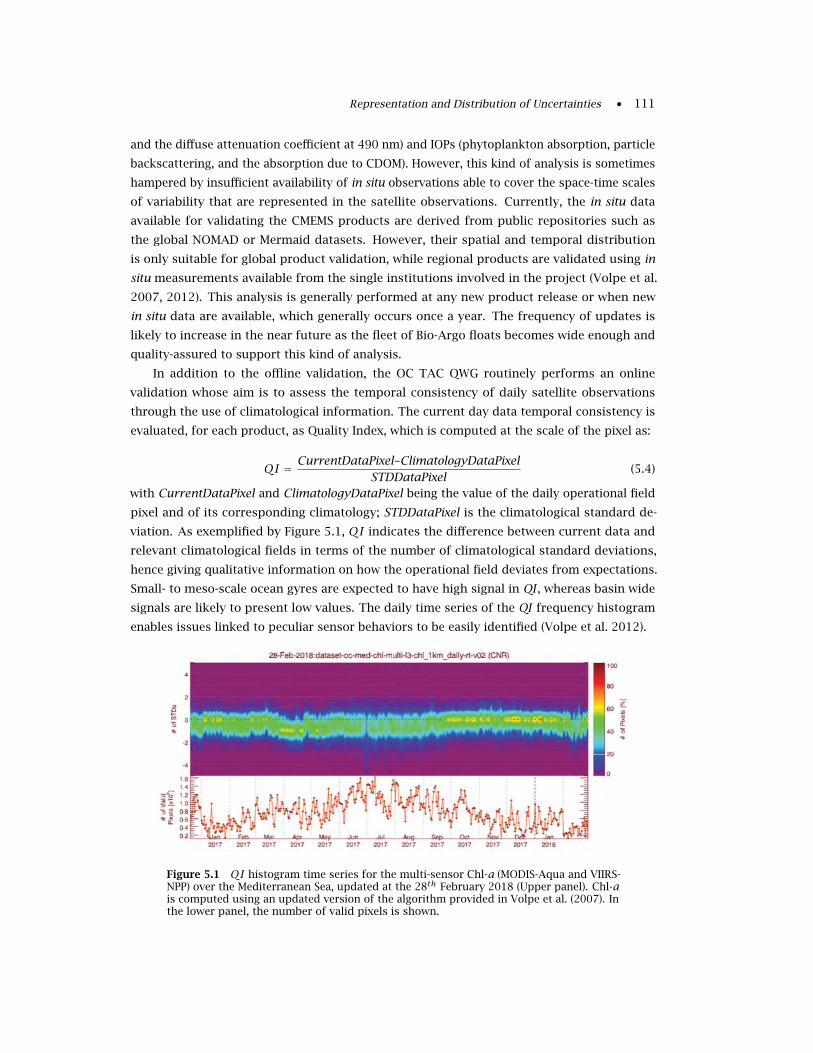
Representation and Distribution of Uncertainties • 111
and the diffuse attenuation coefficient at 490 nm) and IOPs (phytoplankton absorption, particle
backscattering, and the absorption due to CDOM). However, this kind of analysis is sometimes
hampered by insufficient availability of in situ observations able to cover the space-time scales
of variability that are represented in the satellite observations. Currently, the in situ data
available for validating the CMEMS products are derived from public repositories such as
the global NOMAD or Mermaid datasets. However, their spatial and temporal distribution
is only suitable for global product validation, while regional products are validated using in
situ measurements available from the single institutions involved in the project (Volpe et al.
2007, 2012). This analysis is generally performed at any new product release or when new
in situ data are available, which generally occurs once a year. The frequency of updates is
likely to increase in the near future as the fleet of Bio-Argo floats becomes wide enough and
quality-assured to support this kind of analysis.
In addition to the offline validation, the OC TAC QWG routinely performs an online
validation whose aim is to assess the temporal consistency of daily satellite observations
through the use of climatological information. The current day data temporal consistency is
evaluated, for each product, as Quality Index, which is computed at the scale of the pixel as:
QI = CurrentDataPixel–ClimatologyDataPixelSTDDataPixel
(5.4)
with CurrentDataPixel and ClimatologyDataPixel being the value of the daily operational field
pixel and of its corresponding climatology; STDDataPixel is the climatological standard de-
viation. As exemplified by Figure 5.1, QI indicates the difference between current data and
relevant climatological fields in terms of the number of climatological standard deviations,
hence giving qualitative information on how the operational field deviates from expectations.
Small- to meso-scale ocean gyres are expected to have high signal in QI , whereas basin wide
signals are likely to present low values. The daily time series of the QI frequency histogram
enables issues linked to peculiar sensor behaviors to be easily identified (Volpe et al. 2012).
Figure 5.1 QI histogram time series for the multi-sensor Chl-a (MODIS-Aqua and VIIRS-NPP) over the Mediterranean Sea, updated at the 28th February 2018 (Upper panel). Chl-ais computed using an updated version of the algorithm provided in Volpe et al. (2007). Inthe lower panel, the number of valid pixels is shown.

112 • Uncertainties in Ocean Colour Remote Sensing
Chapter 6
Requirements for Different Applications of Ocean Colour
Data
Stephanie Dutkiewicz, Prakash Chauhan, David Ford, Thomas Jackson, Emlyn
Jones, Samantha Lavender, Victor Martinez-Vicente, Frédéric Mélin, Marie-Fanny
Racault, Shubha Sathyendranath, Himmatsinh U. Solanki and Guangming Zheng
Ocean colour has a wide range of applications (IOCCG 2008), in relation to numerical models,
climate research, environmental monitoring and phenological or ecosystem studies. The
uncertainty requirements of each of these applications is likely to be different. As many of
the users in these communities are not ocean colour experts, they are often unaware of the
levels of uncertainties in the products they are using. Thus, when distributing products, it
is particularly important to include uncertainty estimates accompanied by clear and concise
descriptions of what the uncertainty terms represent. Before illustrating non-exhaustive
examples of requirements for specific communities or applications, a short note of the current
mission uncertainty requirements (or objectives) is provided.
6.1 Mission Objectives
Comprehensive mission requirements are defined according to the science questions that need
to be resolved (IOCCG 2012). Some requirements have been phrased in terms of objectives
related to uncertainties. For instance, the following objectives were set for SeaWiFS (McClain
et al. 1992):
• Radiometric accuracy to within 5% absolute and 1% relative
• Water-leaving radiance to within 5% absolute
• Chlorophyll-a concentration to within 35% over the range 0.05–50 mg m−3
• Global primary production to within 50% absolute with a precision to within 10%,
with Hooker and McClain (2000) explicitly stating that the 5% objective for Lw is for clear waters.
These objectives on Lw and Chl-a have been adopted in a large measure by the following
satellite missions and have made their way to the GCOS requirements (see Section 6.4 below).
For instance, requirements for products from OLCI on-board Sentinel-3 are (Drinkwater and
Rebhan 2017):
• Accuracy for marine reflectance of 5× 10⁻⁴ (in the range 0.001–0.004) for both Case-1
and Case-2 waters,
113
114 • Uncertainties in Ocean Colour Remote Sensing
• Accuracy for water-leaving radiance of 5% (up to 1 mW cm−2 µm−1 sr−1) for both Case-1
and Case-2 waters,
• Accuracy for Chl-a (in the range 0.001–150 mg m−3) and for TSM (in the range 0–100 g
m−3) of 30% (threshold) and 10% (goal) for Case-1 waters, 70% (threshold) and 10% (goal)
for Case-2 waters,
• Accuracy for Kd (in the range 0.001–0.1 m−1) of 5% in both Case-1 and Case-2 waters,
• Accuracy for CDOM absorption (412 nm, in the range 0.01–2 m−1) of 50% (threshold)
and 10% (goal) for Case-1 waters, 70% (threshold) and 10% (goal) for Case-2 waters,
• Accuracy for PAR (in the range 0 to 1400 µmol m−2 s−1) of 5%.
For the PACE (Plankton, Aerosol, Cloud, ocean Ecosystem) mission, uncertainty objectives for
water reflectance are expressed as the maximum of a relative value (in %) and an absolute
value (i.e., in reflectance, given in brackets): 20% (0.0057), 5% (0.0020), and 10% (0.0007) in the
spectral ranges 350–400, 400–600, and 600–700 nm, respectively (Werdell et al. 2019).
It should be noted that in metrological vocabulary the accuracy often found in mission
documentation refers to the closeness of agreement between a measured value and the true
value (Chapter 2); in that context it would be more appropriate to state mission objectives in
terms of uncertainties.
6.2 Users Requirements
When it come to uncertainties, user requirements can be extremely varied following each
application or research objective and compilation efforts are welcome. For instance, the OC
user community needs have been assessed within several projects funded by ESA, with the aim
of defining the required characteristics of satellite derived biogeochemical products. In 2010,
the ESA Ocean Colour Climate Change Initiative (OC-CCI) project collected views from the
scientific community using an on-line survey and workshop; in the resulting User Requirements
Document, the analysis of the respondents was separated into modellers and Earth Observation
(EO) scientists. Specifically, respondents were asked about product spatial and temporal
resolution, stability and data access as well as uncertainty (OC-CCI 2016; Sathyendranath et al.
2019). Requirements were divided into “threshold” (minimum requirement to be met to ensure
that data are useful), “goal” (an ideal requirement, above which further improvements are not
necessary) and “breakthrough” (an intermediate level between “threshold” and “goal” which, if
achieved, would result in a significant improvement for the targeted application). Requested
uncertainties were quantified in relative terms (%) by systematic and random contributions
to the uncertainty budget, termed “accuracy” (taken as an estimate of systematic error) and
“precision” (taken as an estimate of the random error). It can be noted here that this vocabulary
does not fully coincide with that introduced in Chapter 2 for metrological definitions.
Typical requested uncertainties are in the range 10–25% for Chl-a. The same range is given
for LWN (or RRS ) within the modelling community (however this value should be interpreted
with care as few modellers use RRS directly) while values less than 10% are requested by EO
scientists. The survey included other OC variables such IOPs, Kd or PFTs. Regardless of the
Requirements for Different Applications of Ocean Colour Data • 115
stated uncertainties, an almost unanimous requirement emerging from the survey was the
necessity of accompanying OC products with uncertainty estimates.
The ESA Pools of Carbon in the Ocean (POCO) project followed up from OC-CCI, attempting
to identify the priorities in the development of algorithms that retrieve carbon pools from
ocean colour. To this end, an on-line questionnaire was designed and circulated among
the ocean colour and modelling communities. Methodology and responses are detailed
elsewhere (POCO 2015). The products of interest for the communities were (in descending
order of interest): phytoplankton carbon, particulate organic carbon, particulate inorganic
carbon, total particulate carbon and dissolved organic carbon. Given the novelty of these
products, uncertainty was not separated in specific components. Instead, an aggregate question
concerning uncertainty in products related to carbon pools was posed to the respondents,
with half of the respondents requiring an uncertainty level of 10–25%. Similarly to the OC-CCI,
uncertainty estimates were required alongside the absolute values of the product.
Increasingly, users are requesting that products be self-evaluated against a set of require-
ments to establish their levels of maturity. Different user groups have established “maturity
index” tables to standardise the responses of product providers to such needs. The maturity
matrix produced by the European Union project CORE-CLIMAX (Su et al. 2018) places conside-
rable importance on the uncertainty characterization available for the product, as an essential
ingredient for establishing its maturity (see also Section 6.4).
On the other hand, some applications might be less demanding in terms of quantitative
uncertainties. Some analyses addressing bloom detection and area estimation, or river plume
monitoring, may focus more on the detection of specific features or contrasts (e.g., Gower
et al. 2006; Hu et al. 2010; Blondeau-Patissier et al. 2014; Fernández-Nóvoa et al. 2015; Qi et al.
2017a; Urquhart et al. 2017). Some physical applications actually need only values of gradients,
for instance to detect fronts and eddies (Wall et al. 2008; Belkin and O’Reilly 2009) or specific
oceanographic features linked to internal waves or turbulence structures (da Silva et al. 2002;
Skákala and Smyth 2015). Similarly (temporal) feature tracking OC analyses, as applied to
current estimation (Liu et al. 2002; Jiang and Wang 2017) or ice drift (Lang et al. 2014), do
not require highly quantitative OC estimates. Studies on oil spill detection also puts more
emphasis on contrast detection in OC data (Hu et al. 2009; Bulgarelli and Djavidnia 2012).
In the rest of this chapter we highlight some illustrative user communities and their
associated uncertainty challenges.
6.3 Numerical Biogeochemical/Ecosystem Modeling
Numerical biogeochemical and ecosystem models, including those involved in climate simulati-
ons, frequently use OC products for evaluation. In general terms, observational data need to
be accompanied by uncertainty estimates to provide a context for the model-data comparison;
only in that case can differences between model outputs and data be confidently appreciated.
Additionally, over the last decade, some numerical models have been using OC products in
data assimilation (e.g., Gregg 2008; Shulman et al. 2013; Ciavatta et al. 2014; Jones et al. 2016;
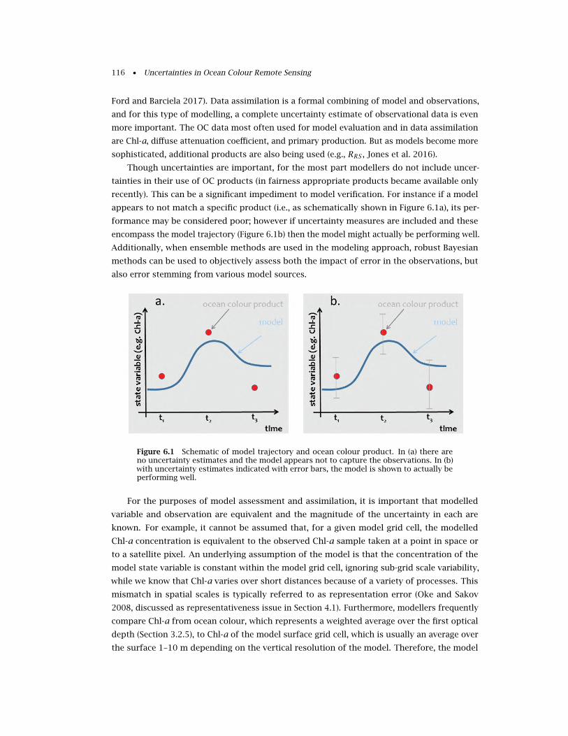
116 • Uncertainties in Ocean Colour Remote Sensing
Ford and Barciela 2017). Data assimilation is a formal combining of model and observations,
and for this type of modelling, a complete uncertainty estimate of observational data is even
more important. The OC data most often used for model evaluation and in data assimilation
are Chl-a, diffuse attenuation coefficient, and primary production. But as models become more
sophisticated, additional products are also being used (e.g., RRS , Jones et al. 2016).
Though uncertainties are important, for the most part modellers do not include uncer-
tainties in their use of OC products (in fairness appropriate products became available only
recently). This can be a significant impediment to model verification. For instance if a model
appears to not match a specific product (i.e., as schematically shown in Figure 6.1a), its per-
formance may be considered poor; however if uncertainty measures are included and these
encompass the model trajectory (Figure 6.1b) then the model might actually be performing well.
Additionally, when ensemble methods are used in the modeling approach, robust Bayesian
methods can be used to objectively assess both the impact of error in the observations, but
also error stemming from various model sources.
Figure 6.1 Schematic of model trajectory and ocean colour product. In (a) there areno uncertainty estimates and the model appears not to capture the observations. In (b)with uncertainty estimates indicated with error bars, the model is shown to actually beperforming well.
For the purposes of model assessment and assimilation, it is important that modelled
variable and observation are equivalent and the magnitude of the uncertainty in each are
known. For example, it cannot be assumed that, for a given model grid cell, the modelled
Chl-a concentration is equivalent to the observed Chl-a sample taken at a point in space or
to a satellite pixel. An underlying assumption of the model is that the concentration of the
model state variable is constant within the model grid cell, ignoring sub-grid scale variability,
while we know that Chl-a varies over short distances because of a variety of processes. This
mismatch in spatial scales is typically referred to as representation error (Oke and Sakov
2008, discussed as representativeness issue in Section 4.1). Furthermore, modellers frequently
compare Chl-a from ocean colour, which represents a weighted average over the first optical
depth (Section 3.2.5), to Chl-a of the model surface grid cell, which is usually an average over
the surface 1–10 m depending on the vertical resolution of the model. Therefore, the model
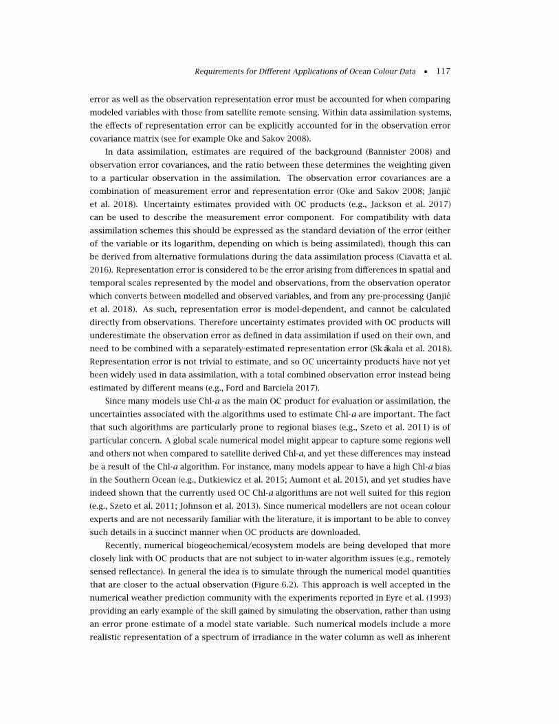
Requirements for Different Applications of Ocean Colour Data • 117
error as well as the observation representation error must be accounted for when comparing
modeled variables with those from satellite remote sensing. Within data assimilation systems,
the effects of representation error can be explicitly accounted for in the observation error
covariance matrix (see for example Oke and Sakov 2008).
In data assimilation, estimates are required of the background (Bannister 2008) and
observation error covariances, and the ratio between these determines the weighting given
to a particular observation in the assimilation. The observation error covariances are a
combination of measurement error and representation error (Oke and Sakov 2008; Janjic
et al. 2018). Uncertainty estimates provided with OC products (e.g., Jackson et al. 2017)
can be used to describe the measurement error component. For compatibility with data
assimilation schemes this should be expressed as the standard deviation of the error (either
of the variable or its logarithm, depending on which is being assimilated), though this can
be derived from alternative formulations during the data assimilation process (Ciavatta et al.
2016). Representation error is considered to be the error arising from differences in spatial and
temporal scales represented by the model and observations, from the observation operator
which converts between modelled and observed variables, and from any pre-processing (Janjic
et al. 2018). As such, representation error is model-dependent, and cannot be calculated
directly from observations. Therefore uncertainty estimates provided with OC products will
underestimate the observation error as defined in data assimilation if used on their own, and
need to be combined with a separately-estimated representation error (Skákala et al. 2018).
Representation error is not trivial to estimate, and so OC uncertainty products have not yet
been widely used in data assimilation, with a total combined observation error instead being
estimated by different means (e.g., Ford and Barciela 2017).
Since many models use Chl-a as the main OC product for evaluation or assimilation, the
uncertainties associated with the algorithms used to estimate Chl-a are important. The fact
that such algorithms are particularly prone to regional biases (e.g., Szeto et al. 2011) is of
particular concern. A global scale numerical model might appear to capture some regions well
and others not when compared to satellite derived Chl-a, and yet these differences may instead
be a result of the Chl-a algorithm. For instance, many models appear to have a high Chl-a bias
in the Southern Ocean (e.g., Dutkiewicz et al. 2015; Aumont et al. 2015), and yet studies have
indeed shown that the currently used OC Chl-a algorithms are not well suited for this region
(e.g., Szeto et al. 2011; Johnson et al. 2013). Since numerical modellers are not ocean colour
experts and are not necessarily familiar with the literature, it is important to be able to convey
such details in a succinct manner when OC products are downloaded.
Recently, numerical biogeochemical/ecosystem models are being developed that more
closely link with OC products that are not subject to in-water algorithm issues (e.g., remotely
sensed reflectance). In general the idea is to simulate through the numerical model quantities
that are closer to the actual observation (Figure 6.2). This approach is well accepted in the
numerical weather prediction community with the experiments reported in Eyre et al. (1993)
providing an early example of the skill gained by simulating the observation, rather than using
an error prone estimate of a model state variable. Such numerical models include a more
realistic representation of a spectrum of irradiance in the water column as well as inherent
118 • Uncertainties in Ocean Colour Remote Sensing
optical properties (e.g., Gregg and Rousseaux 2014; Xiu and Chai 2014; Dutkiewicz et al. 2015;
Baird et al. 2016). Even without resolving a complex radiative transfer component, it is possible
with varying assumptions to implement an optical module in a post-processing step (e.g.,
Baird et al. 2016). The optical module in the numerical model uses physics-based equations
to estimate the IOPs and AOPs and relies on few empirical-statistical relationships. Taking
into account their vertical distribution and spectral characteristics, these optical properties
can be directly related to satellite derived remote sensing products such as reflectance RRS ,a radiometric quantity the uncertainties of which are more tractable compared to products
obtained through empirical algorithms such as standard Chl-a. By adopting this approach,
numerical models are no longer constrained to comparing modeled Chl-a with Chl-a derived
from an OC satellite platform. On the other hand they have to account for the uncertainties
associated with their internal optical model and parameters.
BGC Model Variable(plankton biomass,
nutrients, detritus, Chl-a)
IOPs(absorp�on and
sca�ering)
AOPs(radiance / reflectance)
Derived Products(simulated Chl-a,
simulated true color)
Satellite observa�ons(top of atmosphere
radiance)
AOPs(radiance / reflectance)
AOPs(Kd)
IOPs
Derived Products(Chl-a, true color,
POC, PFT’s)
Figure 6.2 The flow chart of how the model state variables are transformed into IOPsand AOPs compared with the satellite data processing flow.
By simulating directly observable radiometric quantities and circumventing the need to
rely on empirical statistical relationships to convert AOPs to derived Chl-a products, there is
Requirements for Different Applications of Ocean Colour Data • 119
now the opportunity to also make use of newly commissioned satellites, that may not be tuned
specifically for ocean colour. An example of this is Himawari-8, which is primarily used for
meteorological purposes. It does however, have 3 bands dedicated to true color that can be
used for model assessment and assimilation.
6.4 Climate Research
The primary requirements related to climate science for ocean colour are distributed by the
Global Climate Observing System (GCOS). GCOS is co-sponsored by the World Meteorological
Organization (WMO), the Intergovernmental Oceanographic Commission (IOC) of the United
Nations Educational, Scientific and Cultural Organization (UNESCO), the United Nations En-
vironment Programme (UNEP) and the International Council for Science (ICSU). It reports on
the status of the current climate observing capabilities to the United Nations Framework
Convention on Climate Change (UNFCCC). GCOS has identified a set of 54 Essential Climate
Variables (ECVs), the measurements of which exert a high impact on the requirements of the
UNFCCC and climate science. A large part of these ECVs can be determined using space-based
observations, and GCOS recognizes the importance of satellite remote sensing to provide
global observations required for climate science.
GCOS has defined general Climate Monitoring Principles and requirements for data streams,
the fulfilment of which would efficiently support climate science objectives. Relevant to the
issue of uncertainties are a focus on the calibration of the instruments and the operation of in
situ baseline observations. Ultimately, “random errors and time-dependent biases in satellite
observations and derived products should be identified” (GCOS 2011). For each ECV, GCOS
has fixed specific requirements in terms of resolution and uncertainties (GCOS 2011); these
requirements are targets considered sufficient for current climate applications. Two ECVs
are derived from OC remote sensing, water leaving radiance Lw (also termed ocean colour
radiometry) and chlorophyll-a concentration, with the TOA radiance acting as Fundamental
Climate Data Record (FCDR). Table 6.1 reproduces the associated GCOS requirements. In
the original table, the heading for “uncertainty” is actually expressed as “accuracy”, while
GUM (2008) defines “accuracy” as the closeness of agreement between the product value and
the (unknown) true value (Chapter 2). Under that heading are requirements “indicative of
acceptable overall levels for the uncertainties of product values” (GCOS 2011). Values under the
“stability” heading refer to “the maximum acceptable change in systematic error per decade”.
It is important to notice that the requirements are associated with specific resolution, in time
(daily and weekly for Lw and Chl-a, respectively) and space (4-km and 30-km, respectively). It
is however acknowledged that kilometer or sub-kilometer resolution might be necessary for
coastal and regional applications. The uncertainty of 5% for Lw is intended for the blue and
green spectral domain in Case-1 waters; similarly, the uncertainty for Chl-a (35%) is given for
Case-1 waters in the range 0.01–10 mg m−3. It is recalled here that the stated uncertainties for
Lw and Chl-a (even though expressed for different resolutions) can be related, for instance by
considering simple band-ratio empirical algorithms (e.g., Gordon and Clark 1981).
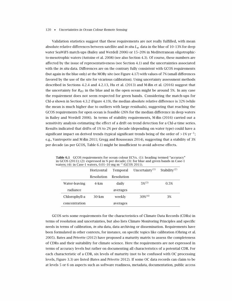
120 • Uncertainties in Ocean Colour Remote Sensing
Validation statistics suggest that these requirements are not really fulfilled, with mean
absolute relative differences between satellite and in situ Lw data in the blue of 10–13% for deep
water SeaWiFS match-ups (Bailey and Werdell 2006) or 15–20% in Mediterranean oligotrophic-
to-mesotrophic waters (Antoine et al. 2008) (see also Section 4.3). Of course, these numbers are
affected by the issue of representativeness (see Section 4.1) and the uncertainties associated
with the in situ data. Differences are on the contrary fully consistent with GCOS requirements
(but again in the blue only) at the MOBy site (see Figure 4.17) with values of 7% (small differences
favored by the use of the site for vicarious calibration). Using uncertainty assessment methods
described in Sections 4.2.4 and 4.2.13, Hu et al. (2013) and Mélin et al. (2016) suggest that
the uncertainty for RRS in the blue and in the open ocean might be around 5%. In any case
the requirement does not seem respected for green bands. Considering the match-ups for
Chl-a shown in Section 4.3.2 (Figure 4.19), the median absolute relative difference is 32% (while
the mean is much higher due to outliers with large residuals), suggesting that reaching the
GCOS requirements for open ocean is feasible (26% for the median difference in deep waters
in Bailey and Werdell 2006). In terms of stability requirements, Mélin (2016) carried out a
sensitivity analysis estimating the effect of a drift on trend detection for a Chl-a time series.
Results indicated that drifts of 1% to 2% per decade (depending on water type) could have a
significant impact on derived trends (typical significant trends being of the order of >1% yr−1;
e.g., Vantrepotte and Mélin 2011; Gregg and Rousseaux 2014), suggesting that a stability of 3%
per decade (as per GCOS, Table 6.1) might be insufficient to avoid adverse effects.
Table 6.1 GCOS requirements for ocean colour ECVs. (1): heading termed “accuracy”in GCOS (2011); (2): expressed in % per decade; (3): for blue and green bands in Case-1waters; (4): in Case-1 waters, 0.01–10 mg m−3 (GCOS 2011).
Horizontal Temporal Uncertainty(1) Stability(2)
Resolution Resolution
Water-leaving 4-km daily 5%(3) 0.5%
radiance averages
Chlorophyll-a 30-km weekly 30%(4) 3%
concentration averages
GCOS sets some requirements for the characteristics of Climate Data Records (CDRs) in
terms of resolution and uncertainties, but also lists Climate Monitoring Principles and specific
needs in terms of calibration, in situ data, data archiving or dissemination. Requirements have
been formulated in other contexts, for instance, on specific topics like calibration (Ohring et al.
2005). Bates and Privette (2012) have proposed a maturity matrix to assess the completeness
of CDRs and their suitability for climate science. Here the requirements are not expressed in
terms of accuracy levels but rather on documenting all characteristics of a potential CDR. For
each characteristic of a CDR, six levels of maturity (not to be confused with OC processing
levels, Figure 3.3) are listed (Bates and Privette 2012). If some OC data records can claim to be
at levels 5 or 6 on aspects such as software readiness, metadata, documentation, public access
Requirements for Different Applications of Ocean Colour Data • 121
and utility, this is generally not the case for product validation for which the levels are defined
as:
1. little or none,
2. minimal,
3. uncertainty estimated for select locations/times,
4. uncertainty estimated over widely distributed times/locations by multiple investigators;
differences understood,
5. consistent uncertainties estimated over most environmental conditions by multiple
investigators,
6. observation strategy designed to reveal systematic errors through independent cross-
checks, open inspection, and continuous interrogation; quantified errors.
It could be argued that OC remote sensing is qualifying for levels 3 to 4 with some elements of
level 6, depending on which variable is considered. Along the same line, a System Maturity
Matrix has been proposed by the CORE-CLIMAX project (Merchant et al. 2017; Su et al. 2018;
Nightingale et al. 2018) listing different levels of maturity for uncertainty characterization of
CDRs, and a framework is put in place for the European Union’s Copernicus Climate Change
Service (Nightingale et al. 2019). These or similar discussions can provide a formal framework
to assess the status of current CDRs and help in defining future strategies.
6.5 Environmental Monitoring
OC remote sensing offers a portfolio of products with applications to environmental or
water quality monitoring, describing water clarity/turbidity, phytoplankton (represented by
concentration of pigments or the detection of algal blooms), suspended sediments, dissolved
material, Secchi Disk depth, light availability for submerged vegetation etc. (Zheng and
DiGiacomo 2017; IOCCG 2018). These products are often derived with empirical or semi-
analytical bio-optical algorithms for which uncertainty calculations can follow the principles
described in Section 4.2. For the sake of illustration, two common products, turbidity in
Nephelometric Turbidity Units (NTUs) and chlorophyll concentration, are discussed here in the
context of specific regulations.
Arguably the most mature (for instance from a U.S. regulatory standpoint) water quality
parameter that can be derived remotely is turbidity. Turbidity (in various nephelometric units)
has been used to indicate water quality for many years by the U.S. Environmental Protection
Agency. Higher turbidity levels are often associated with higher levels of disease-causing
microorganisms, or pathogens, such as viruses, bacteria, and protozoan parasites. In the
U.S., surface water turbidity standards vary from state to state, and may differ among water
bodies within a state. In addition, many standards are given in terms of absolute values of
turbidity exceedance rather than in percentage, making it difficult to propose percent-wise
uncertainty requirements. For example, Alaska requires that aquaculture-induced turbidity
increase “may not exceed 25 NTU above natural conditions” except for all lake waters where no
122 • Uncertainties in Ocean Colour Remote Sensing
exceedance above 5 NTU is allowed 1. Florida requires that turbidity “shall not exceed 29 NTUs
above natural background conditions”. However, restrictions on percent-wise exceedance are
sometimes provided. For example, Alaska and Washington states both forbid >10% artificial
increase in turbidity when the background turbidity is more than 50 NTU for waters designated
for higher use purposes, or >20% increase for lower use purposes. This is also consistent
with federally promulgated water quality standards for Colville Confederated Tribes Indian
Reservation (U.S. Code of Federal Regulations: 40 C.F.R. 131.35, 20182). To summarize, if
satellite-derived turbidity products were to be used for environmental compliance purposes,
relevant regulations on maximum exceedance relative to the limit must be taken into account
to determine “threshold”, “breakthrough”, and “goal” uncertainty requirements. And these
requirements will be site-specific.
Another important satellite water quality product is the chlorophyll concentration, the
regulation of which has recently undergone rapid development for instance in the U.S.3.
While total nitrogen and total phosphorus criteria are preferable for directly determining
eutrophication status and nutrients discharge limits, chlorophyll can be considered as an
indicator of the direct effect of nutrient enrichment. Like turbidity standards, chlorophyll-a
standards in the U.S. are also site-specific. Taking state regulations for estuaries for example,
the upper limit for chlorophyll-a concentration is 15 mg m−3 in Oregon, 40 mg m−3 in
North Carolina, 10–23 mg m−3 in Virginia, 0.3–8.2 mg m−3 in Florida, and 2–20 mg m−3 in
Hawaii. In Europe, target chlorophyll concentrations/ranges are also determined locally for
different water types and water categories, including coastal and transitional water bodies
(defined in the European Commission Decision 2008/915/EC4). Water types in the coastal
and transitional category were determined based on salinity, tidal range, water depth, current
velocity, stratification and mixing, presence of upwelling, whether the waters are sheltered,
enclosed, exposed, fjordic, etc. For the Baltic Sea region, the “High-Good” and “Good-Moderate”
quality boundaries in summer are defined as 1.1–4.3 mg m−3 and 1.6–5.8 mg m−3, respectively,
across different water types. In the North East Atlantic region, these two boundaries are 1–10
mg m−3 and 2–15 mg m−3, respectively. So in the case of satellite-derived chlorophyll product,
the required threshold uncertainty can be determined by calculating the difference between
regulatory limit and most-frequently observed values at a given site. To be able to give a
definitive answer for most cases, the uncertainty shall not surpass the difference normalized
by the regulatory limit.
6.6 Phenology Studies
Phenology relates to the study of timing of events in the periodic growth of phytoplankton
populations as influenced by the environment. A number of phenological indices have been
1https://archive.epa.gov/epa/wqc/developing-water-quality-criteria-suspended-and-bedded-sediments-sabs.
html2www.ecfr.gov/cgi-bin/text-idx?SID=454a7b51118b27f20cef29ff071c1440&node=40:22.0.1.1.18&rgn=div53www.epa.gov/nutrient-policy-data/state-progress-toward-developing-numeric-nutrient-water-quality-criteria4http://eur-lex.europa.eu/LexUriServ/LexUriServ.do?uri=OJ:L:2008:332:0020:0044:EN:PDF
Requirements for Different Applications of Ocean Colour Data • 123
developed to describe the annual cycle of phytoplankton from OC remote sensing observations
(Platt and Sathyendranath 1996, 2008), including the timings of initiation, peak, termination
and duration of the phytoplankton growing period in a given season. These indices carry out
units of time (i.e., days, weeks or months). They are not sensitive to errors in the absolute
values of chlorophyll, and less stringent requirements may apply, which make them particularly
relevant to study long-term changes in phytoplankton seasonality based on different OC
sensors.
The timing of the peak in the phytoplankton growing period corresponds to the time when
Chl-a reaches maximum amplitude in the annual cycle. The duration of the growing period
is estimated as the time elapsed between the timings of initiation and termination. Several
methods have been proposed to estimate the timings of initiation and termination (see Ji et al.
2010 for a review). Conventionally, the methods involve a threshold criterion, which provides
a boundary value to delineate initiation and termination of a phytoplankton growing period.
The threshold criterion can be estimated directly from the remotely-sensed Chl-a time-series
(Siegel et al. 2002a; Henson et al. 2006; Thomalla et al. 2011; Racault et al. 2012), or after
fitting a density function to the Chl-a time-series (Platt et al. 2009; Vargas et al. 2009; Zhai
et al. 2011; Sapiano et al. 2012; González Taboada and Anadón 2014; Ardyna et al. 2014), or
performing a cumulative summation of Chl-a (Brody et al. 2013) or Chl-a anomalies (Racault
et al. 2015, 2017). Although different methods and threshold criteria may yield similar results
(Brody et al. 2013; Ferreira et al. 2014), the choice of method and threshold requires scrutiny of
the shape of the phytoplankton annual cycle and consideration of the research question being
investigated. Once the method is chosen, implementation of phenological studies does require
data well distributed in time (i.e., with few missing data), to enable resolution of timings of
seasonal events with sufficient accuracy (Cole et al. 2012; Land et al. 2014; Racault et al. 2014;
Ferreira et al. 2014).
Missing data arise when the retrieval of remote-sensing reflectance is limited by Sun glint,
clouds, atmospheric aerosol, high solar zenith angle or other excluding conditions. In addition,
during the first OC exploratory mission, performed by the Coastal Zone Color Scanner (CZCS,
1978–1986), the collection of observations was limited for all the reasons above, and also by
power and data recorder limitations, which led to the priority being set on observations in the
coastal regions and in the Northern Hemisphere. An example of estimation of uncertainty in
phenological indices associated with missing data in the CZCS archive is provided in Figure
6.3. When the percentage of missing data is less than 60%, the RMSD in estimates of duration
and timing of initiation is shown to drop below 30% and 30 days respectively, and the bias
(representing systematic effects) drops below 10% and 10 days respectively (Racault et al.
2014). Moreover, the bias in the duration is found to be negative throughout the global oceans,
indicating that the duration tends to be under-estimated when data are missing. Using a
different approach, Cole et al. (2012) estimated the differences between phenology metrics
from a multi-mission remote-sensing time-series (GlobColour, Section 5.3.2) and those from
the NASA Ocean Biogeochemical Model (treated as a gap-free time series). They showed that in
sub-polar regions, where the percentage of missing data is high, typical differences of 30 days
for the timing of initiation were found, whereas in the tropics and the subtropics, where the
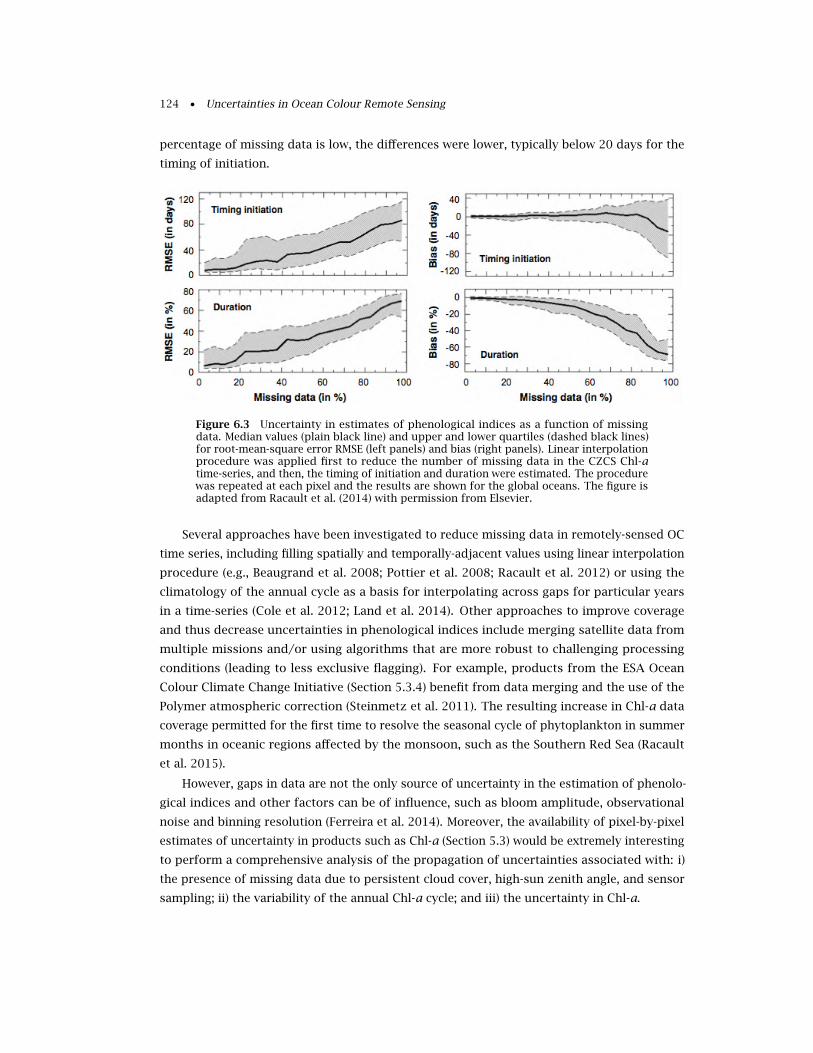
124 • Uncertainties in Ocean Colour Remote Sensing
percentage of missing data is low, the differences were lower, typically below 20 days for the
timing of initiation.
Figure 6.3 Uncertainty in estimates of phenological indices as a function of missingdata. Median values (plain black line) and upper and lower quartiles (dashed black lines)for root-mean-square error RMSE (left panels) and bias (right panels). Linear interpolationprocedure was applied first to reduce the number of missing data in the CZCS Chl-atime-series, and then, the timing of initiation and duration were estimated. The procedurewas repeated at each pixel and the results are shown for the global oceans. The figure isadapted from Racault et al. (2014) with permission from Elsevier.
Several approaches have been investigated to reduce missing data in remotely-sensed OC
time series, including filling spatially and temporally-adjacent values using linear interpolation
procedure (e.g., Beaugrand et al. 2008; Pottier et al. 2008; Racault et al. 2012) or using the
climatology of the annual cycle as a basis for interpolating across gaps for particular years
in a time-series (Cole et al. 2012; Land et al. 2014). Other approaches to improve coverage
and thus decrease uncertainties in phenological indices include merging satellite data from
multiple missions and/or using algorithms that are more robust to challenging processing
conditions (leading to less exclusive flagging). For example, products from the ESA Ocean
Colour Climate Change Initiative (Section 5.3.4) benefit from data merging and the use of the
Polymer atmospheric correction (Steinmetz et al. 2011). The resulting increase in Chl-a data
coverage permitted for the first time to resolve the seasonal cycle of phytoplankton in summer
months in oceanic regions affected by the monsoon, such as the Southern Red Sea (Racault
et al. 2015).
However, gaps in data are not the only source of uncertainty in the estimation of phenolo-
gical indices and other factors can be of influence, such as bloom amplitude, observational
noise and binning resolution (Ferreira et al. 2014). Moreover, the availability of pixel-by-pixel
estimates of uncertainty in products such as Chl-a (Section 5.3) would be extremely interesting
to perform a comprehensive analysis of the propagation of uncertainties associated with: i)
the presence of missing data due to persistent cloud cover, high-sun zenith angle, and sensor
sampling; ii) the variability of the annual Chl-a cycle; and iii) the uncertainty in Chl-a.
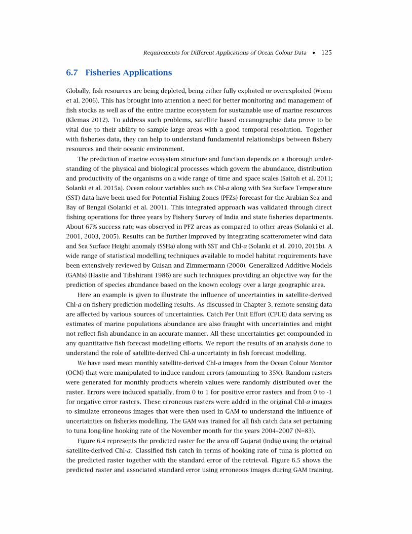
Requirements for Different Applications of Ocean Colour Data • 125
6.7 Fisheries Applications
Globally, fish resources are being depleted, being either fully exploited or overexploited (Worm
et al. 2006). This has brought into attention a need for better monitoring and management of
fish stocks as well as of the entire marine ecosystem for sustainable use of marine resources
(Klemas 2012). To address such problems, satellite based oceanographic data prove to be
vital due to their ability to sample large areas with a good temporal resolution. Together
with fisheries data, they can help to understand fundamental relationships between fishery
resources and their oceanic environment.
The prediction of marine ecosystem structure and function depends on a thorough under-
standing of the physical and biological processes which govern the abundance, distribution
and productivity of the organisms on a wide range of time and space scales (Saitoh et al. 2011;
Solanki et al. 2015a). Ocean colour variables such as Chl-a along with Sea Surface Temperature
(SST) data have been used for Potential Fishing Zones (PFZs) forecast for the Arabian Sea and
Bay of Bengal (Solanki et al. 2001). This integrated approach was validated through direct
fishing operations for three years by Fishery Survey of India and state fisheries departments.
About 67% success rate was observed in PFZ areas as compared to other areas (Solanki et al.
2001, 2003, 2005). Results can be further improved by integrating scatterometer wind data
and Sea Surface Height anomaly (SSHa) along with SST and Chl-a (Solanki et al. 2010, 2015b). A
wide range of statistical modelling techniques available to model habitat requirements have
been extensively reviewed by Guisan and Zimmermann (2000). Generalized Additive Models
(GAMs) (Hastie and Tibshirani 1986) are such techniques providing an objective way for the
prediction of species abundance based on the known ecology over a large geographic area.
Here an example is given to illustrate the influence of uncertainties in satellite-derived
Chl-a on fishery prediction modelling results. As discussed in Chapter 3, remote sensing data
are affected by various sources of uncertainties. Catch Per Unit Effort (CPUE) data serving as
estimates of marine populations abundance are also fraught with uncertainties and might
not reflect fish abundance in an accurate manner. All these uncertainties get compounded in
any quantitative fish forecast modelling efforts. We report the results of an analysis done to
understand the role of satellite-derived Chl-a uncertainty in fish forecast modelling.
We have used mean monthly satellite-derived Chl-a images from the Ocean Colour Monitor
(OCM) that were manipulated to induce random errors (amounting to 35%). Random rasters
were generated for monthly products wherein values were randomly distributed over the
raster. Errors were induced spatially, from 0 to 1 for positive error rasters and from 0 to -1
for negative error rasters. These erroneous rasters were added in the original Chl-a images
to simulate erroneous images that were then used in GAM to understand the influence of
uncertainties on fisheries modelling. The GAM was trained for all fish catch data set pertaining
to tuna long-line hooking rate of the November month for the years 2004–2007 (N=83).
Figure 6.4 represents the predicted raster for the area off Gujarat (India) using the original
satellite-derived Chl-a. Classified fish catch in terms of hooking rate of tuna is plotted on
the predicted raster together with the standard error of the retrieval. Figure 6.5 shows the
predicted raster and associated standard error using erroneous images during GAM training.
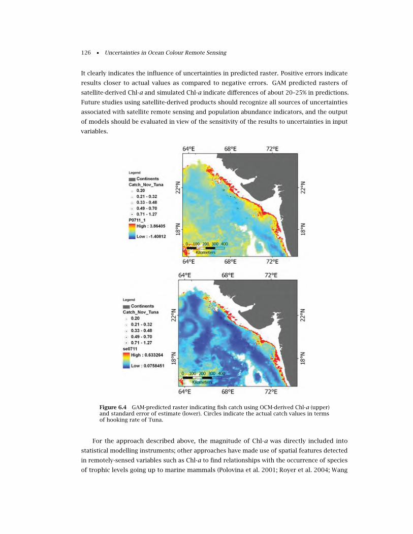
126 • Uncertainties in Ocean Colour Remote Sensing
It clearly indicates the influence of uncertainties in predicted raster. Positive errors indicate
results closer to actual values as compared to negative errors. GAM predicted rasters of
satellite-derived Chl-a and simulated Chl-a indicate differences of about 20–25% in predictions.
Future studies using satellite-derived products should recognize all sources of uncertainties
associated with satellite remote sensing and population abundance indicators, and the output
of models should be evaluated in view of the sensitivity of the results to uncertainties in input
variables.
Figure 6.4 GAM-predicted raster indicating fish catch using OCM-derived Chl-a (upper)and standard error of estimate (lower). Circles indicate the actual catch values in termsof hooking rate of Tuna.
For the approach described above, the magnitude of Chl-a was directly included into
statistical modelling instruments; other approaches have made use of spatial features detected
in remotely-sensed variables such as Chl-a to find relationships with the occurrence of species
of trophic levels going up to marine mammals (Polovina et al. 2001; Royer et al. 2004; Wang
Requirements for Different Applications of Ocean Colour Data • 127
et al. 2010; Panigada et al. 2017). In cases when only the gradient is needed, statistical methods
are immune to systematic relative errors affecting the satellite spatial distributions and in
general fairly robust to uncertainties in Chl-a.
Figure 6.5 GAM-predicted rasters for induced positive and negative errors in originalChl-a images. (a) is prediction of GAM using positively deviated Chl-a values, (b) isprediction of GAM using negatively deviated Chl-a values, (c) and (d) are standard errorsin (a) as well as (b), respectively. Circles indicate the actual catch values in terms ofhooking rate of Tuna.

128 • Uncertainties in Ocean Colour Remote Sensing
Chapter 7
Recommendations
This Chapter lists some recommendations aiming at promoting a better treatment of uncer-
tainties and at reducing the uncertainties associated with ocean colour products, this second
objective depending very much on the first. The focus is on an improved description of uncer-
tainties within the OC community, the creation and dissemination of uncertainty distributions,
and their integration in scientific analyses and other applications. The final objective is to
ensure traceability of OC products to appropriate SI (International System of Units) standards,
meaning a relation to these standards through an unbroken chain of procedures, each contribu-
ting to document uncertainties, ultimately leading to a comprehensive uncertainty budget (VIM
2012). The OC community has gathered large amounts of material on these issues but is still
far from reaching these goals. Developments that could ultimately lead to improved products,
such as better technology for optical sensors, the deployment of optical floats, harnessing new
technology (e.g., Lidar) or more powerful computing facilities, are mostly considered out of the
scope of this Chapter. Itemized below are the major recommendations with prior explanatory
text.
The first recommendation is to adopt and enforce a common terminology appropriate to
describe all issues related to uncertainties. As anticipated in Chapter 2, an obvious choice is to
adopt the vocabulary in use in the metrology community. As this terminology is not necessarily
readily applicable to the situations and issues faced by OC remote sensing, initiatives aiming at
clearly interpreting (“translating”) it in the field of Earth Observation are welcome (e.g., projects
like FIDUCEO, Fidelity and uncertainty in climate data records from Earth Observations 1, or
QA4ECV, Quality Assurance for Essential Climate Variables 2, Nightingale et al. 2018). This
report has already provided a tentative discussion on this topic. An extended dialogue with
communities with expertise on other geophysical variables would also be useful (to benefit
from their experience) and necessary (to avoid that the ocean colour community adopt a
vocabulary different from, for example, aerosol or SST experts). The adoption of well-defined
and agreed terminology and methods would also help the dialogue with the user communities
and foster acceptance of the OC products.
1 ⇒ Adopt an appropriate terminology adapted from, and consistent with, metrology.
A corollary to the first recommendation is to improve the statement of uncertainty require-
ments for missions or project deliverables. Past requirements have often been described in
1http://www.fiduceo.eu2http://www.qa4ecv.eu
129
130 • Uncertainties in Ocean Colour Remote Sensing
rather generic and incomplete terms. Their description should actually follow metrology termi-
nology and also be formulated in unambiguous terms and clear mathematical formulations,
with possible distinctions between random and systematic components, time and space scales
involved, etc.
2 ⇒ State mission or project requirements in unambiguous and complete forms.
The OC community also needs to follow best practices in documenting in a fully transparent
way their field activities and satellite data processing chains (including algorithms and un-
certainty determination). It is better to provide too detailed information (on measurement
procedures or algorithm characteristics) than too little. To be fully integrated in validation
activities, field observations should be accompanied by uncertainty estimates and appropriate
auxiliary information (meta-data). The availability of source codes with proper documenta-
tion, particularly for operational processing chains, favors traceability and is a strong point
supporting the development of techniques to derive uncertainties (the most obvious exam-
ple being the techniques based on automatic, or algorithm, differentiation, Vossbeck et al.
2010; Baydin et al. 2018). Considering that the creation of complete uncertainty budgets
must consider the full processing stream, the point above applies equally to the calibration
procedures, atmospheric corrections and bio-optical algorithms. A logical corollary is that
the data distribution should include TOA uncalibrated data. In general, a tight collaboration
and common practices between investigators working on the calibration of space instruments,
atmospheric corrections, bio-optical algorithms, radiative transfer modelling or deployment of
in situ measurement systems should be promoted.
3 ⇒ Availability of full documentation and source codes for the whole processing chain.
4 ⇒ Distribution of non-calibrated TOA data.
As described in Chapter 3, OC processing is a long chain from uncalibrated TOA data to
derived water products. Work on the uncertainties for the entire chain would benefit from
consistency in processing. For instance, RRS products are usually distributed after bidirecti-
onal normalization, with some assumptions about the water IOPs that are often no longer
considered when RRS is input to bio-optical algorithms. The same is true about bio-optical
relationships sometimes used for atmospheric correction (for instance to take into account
water contributions in the NIR) and not for bio-optical algorithms. The inconsistencies make
the process of uncertainty propagation more cumbersome and might violate principles of
energy conservation.
5 ⇒ Respect overall consistency within the processing chain.
Uncertainty estimates should accompany any data set, from pixel level to higher-level products.
For this, metrology principles should be strictly adhered to, starting from mission planning to
distribution of final products. Calibration modules should produce uncertainties associated
with the TOA data (as Fundamental Climate Data Records, FCDR) with a full model of sensor
uncertainty in flight including error-correlation structure (e.g., Gorroño et al. 2018, to allow
propagation of these uncertainties through the downstream suite of algorithms. Ultimately
Recommendations • 131
traceability should be achieved for the entire processing chain, meaning that the product can
be related to a reference through an unbroken sequence (Chapter 2).
6 ⇒ Include uncertainty estimates associated with each datum (for single pixels and grid
points),
7 ⇒ Application of metrology principles to achieve traceability from TOA data to final
products.
Uncertainty fields should be comprehensive, that is to say, containing contributions from all
known error sources (such as described in Chapter 3) except contributions that are demonstra-
ted to exert a negligible impact on the overall uncertainty budget. However, it is recognized
that this is a daunting task and that the community might well proceed by steps. Uncertainty
fields are already distributed with satellite products (Section 5.3) and this should be encoura-
ged. The fact that current and upcoming products might not be complete in their uncertainty
budgets (e.g., considering only TOA uncertainties) is well accepted as long as this is clearly
communicated to the users. The early availability of uncertainty fields, albeit far from perfect,
will favor their use by the user community and the development of methods to ensure their
proper integration in user applications. However, the possibility that data providers distribute
uncertainty fields including a diverse set of error sources in different forms is a cause for
concern since such a situation is very likely to generate confusion and misunderstanding in
the user community. A dialogue between data providers on the distribution of uncertainty
fields with common characteristics should be promoted.
8 ⇒ Ensure a clear description of the uncertainty fields distributed with satellite data,
particularly from the point of view of the error sources they consider.
9 ⇒ Encourage a dialogue between data providers to promote consistency between distribu-
ted uncertainty fields.
Products distributed to the user community should also contain the right amount of metadata
and all information to propagate uncertainties from level-2 to level-3 (at various compositing
scales) and to more advanced products and indicators (number of pixels used for space binning,
percentage of coverage in each bin, variability, error covariance matrices). As discussed
in Section 5.2, the amount of information about uncertainties required by users might be
extremely diverse, from a simple quality indicator to full covariance matrices. A lot of thinking
will be required to distribute simple and portable, yet complete, information about uncertainty
values for a given application. Achieving success is key to promoting the proper use and
acceptance of the data and their related uncertainties. Beyond the purely technical aspects,
conveying uncertainty on scientific products and diagnostics to downstream users and decision
makers is a challenging task calling for skills in communication science and appropriate
language (Weiss 2003; Fischhoff and Davis 2014). Uncertainty values or probabilities might not
be easy to interpret but this is really an important step to guarantee an appropriate use of data
products. Placing too much faith in a product by ignoring its uncertainty might lead to wrong
decisions and actions and eventually to discrediting this product. On the other hand, it should
be clear to users and decision makers that the uncertainty values associated with data do not
132 • Uncertainties in Ocean Colour Remote Sensing
make them “uncertain” and not worthy of action. A proper use of uncertainty distributions
will require a dialogue between data providers and the user community (Taylor et al. 2015)
with an investment in tools and techniques on how to communicate uncertainties, for instance
relying on infographics (Spiegelhalter et al. 2011).
10 ⇒ Distribution of uncertainty fields allowing diverse applications, from the most advan-
ced, when a full uncertainty propagation is required for expert users, to information
appropriate for end users and decision makers.
As shown in Section 4.2, a number of approaches have already been developed and applied to
derive uncertainty estimates with a spatial and/or temporal resolution. These approaches can
be associated with various categories (based on optical water types, on Monte-Carlo simulations)
and already represent a nice sampling of available techniques for uncertainty determination.
However, the developments in that field should be further encouraged. Considering that
the issue of uncertainty definition and propagation has been studied for a long time and in
disciplines with stringent requirements and the needs for advanced methods (in the field of
safety or insurance), contacts with the corresponding mathematical/statistical community
could be very beneficial and could save a considerable amount of time. In parallel, more effort
should be pursued to understand the pros and cons of the approaches currently available
for ocean colour and to compare their results. Besides the definition of uncertainties, more
emphasis should be given to the issue of the domain of applicability as a function of the
application.
11 ⇒ Further development of techniques to estimate uncertainties of OC products and com-
parison between these approaches.
The propagation of uncertainties from pixel-based estimates to space and time composites has
not been properly addressed in the ocean colour community. The necessary developments
on this issue will require an improved knowledge of the error covariance structure of the OC
fields. As said above and in Section 5.2, the information required at pixel level for a proper
propagation of uncertainty fields into composites will have an impact on size and structure of
data files. A close collaboration with the numerical modelling community could be useful in
that regard, and even necessary if its requirements are to be fully served.
12 ⇒ Investigation on the propagation of uncertainty fields from pixel level into space and
time composites.
Comparison between satellite and field data (usually termed validation) has been historically
the main avenue to obtain uncertainty estimates. The interpretation of comparison results in
terms of uncertainties requires information about the uncertainties associated with the field
data themselves and consideration of the representativeness issue (e.g., mismatch in spatial
scales between field and satellite data, Section 4.1). One could think that field data will be less
needed since uncertainty estimates will be increasingly defined through methods like those
described in Section 4.2 as they become more mature, but this would be deeply erroneous.
Field data will remain a key (actually the only) independent means to ensure verification of
Recommendations • 133
the uncertainty estimates associated with satellite products, and therefore the collection of
high-quality field data should be further supported.
13 ⇒ Availability of field data with uncertainty estimates.
14 ⇒ Quantification of the contribution from imperfect representativeness in comparisons
between satellite and field data.
15 ⇒ Promoting a new paradigm by which field data are increasingly used as independent
means to verify uncertainty estimates associated with satellite data.
Considering the points above, obtaining comprehensive uncertainty budgets is a complex and
multi-faceted problem. Progress on the recommendations listed above could be facilitated
by fully leveraging the OC community’s assets. For instance, there is now a suite of satellite
optical missions offering complementary perspectives (albeit with uneven radiometric quality),
with a gradient of spatial resolutions from meters to a kilometer-scale, together with a
mix of polar-orbiting and geostationary platforms and different wavelength sets. Field data
sampling capabilities are also being extended with systems such as floats and gliders (IOCCG
2011). Together with biogeochemical models of finer resolutions and radiative transfer
models operating as virtual laboratories (e.g., Adams et al. 2016), uncertainty propagation and
upscaling issues can certainly be addressed effectively.
16 ⇒ Fully exploit synergies between different types of satellite missions, new field observati-
ons and modelling capabilities.
As outlined in Chapter 3, the uncertainty of a given product can be split into various compo-
nents, loosely defined as stochastic (as associated with inherent variability within the system,
like noise of the input data), epistemic (or structural) in relation to models and parameters,
and numerical/technical. Other layers are added when data are further edited into space/time
composites. Each component requires specific tools for understanding and improvements. In
the case of the structural uncertainty, processing the same data stream with independent ap-
proaches (the equivalent of ensemble simulations), with their own structures and assumptions,
coupled with systematic comparisons would be certainly fruitful to gain enhanced under-
standing about uncertainty propagation. To obtain ensemble time series of OC products in
general would have additional benefits (Merchant et al. 2017) like exempting users of handling
uncertainty fields and their propagation if the ensemble (through its dispersion) is assumed to
contain the uncertainty associated with the product (see an example for surface temperature
in Morice et al. 2012). Along the same line, the comparison between satellite products from
various missions offers a potential that has been only partially exploited. In that respect, a
strong recommendation is to maintain sufficient overlaps between satellite missions (as found
among the GCOS Climate Monitoring Principles).
17 ⇒ Consider the potential of ensemble OC time series.
18 ⇒ Maintain sufficient overlaps between satellite missions.
Eventually, distributing fully documented uncertainty estimates, comprehensive of all error
sources, adhering to metrology principles (traceable to standards), and in forms readily usable

134 • Uncertainties in Ocean Colour Remote Sensing
for all sorts of user applications, is a formidable challenge requiring substantial efforts. But it
can also be seen as an opportunity to improve the quality of the OC data and the ways they
are treated, enhance their scientific value and strengthen the conclusion derived from their
analysis.
Acronyms and Abbreviations
AAOT Acqua Alta Oceanographic Tower
AC Atmospheric Correction
AE Adjacency Effect
AERONET Aerosol Robotic Network
AOP Apparent Optical Property
BRDF Bidirectional Reflectance Distribution Function
CCI Climate Change Initiative
CDOM Chromophoric Dissolved Organic Matter
CDM Coloured Detrital Material
CDR Climate Data Record
Chl-a Chlorophyll a concentration
CMEMS Copernicus Marine Environment Monitoring Service
CPUE Catch Per Unit Effort
CZCS Coastal Zone Color Scanner
DOC Dissolved Organic Carbon
DU Dobson Unit
ECMWF European Centre for Medium-Range Weather Forecast
ECV Essential Climate Variable
EO Earth Observation
ESA European Space Agency
FCDR Fundamental Climate Data Record
FR Full Resolution
GAC Global Area Coverage
GAM Generalized Additive Model
GCOS Global Climate Observing System
GEO Group on Earth Observations
GUM Guide to the Expression of Uncertainty in Measurement
HA Harmful Algae
HDF Hierarchical Data Format
HPLC High-Performance Liquid Chromatography
ICSU International Council for Science
IFOV Instantaneous Field-Of-View
IOC Intergovernmental Oceanographic Commission
IOP Inherent Optical Property
LUT Look-Up Table
135

136 • Uncertainties in Ocean Colour Remote Sensing
MBR Maximum Band Ratio
MEaSUREs Making Earth System Data Records for Use in Research Environments
MERIS Medium Resolution Imaging Spectrometer
MOBY Marine Optical Buoy
MODIS Moderate Resolution Imaging Spectroradiometer
MSI MultiSpectral Instrument
NAP Non Algal Particle
NASA National Aeronautics and Space Administration
NCEP National Centers for Environmental Predictions
NetCDF Network Common Data Form
nFLH normalized Fluorescence Line Height
NIR Near Infra-Red
NL Noise Level
NN Neural Network
NOMAD NASA bio-Optical Marine Algorithm Data set
NTU Nephelometric Turbidity Unit
NWP Numerical Weather Predictions
OC Ocean Colour
OCI Ocean Colour Index
OCM Ocean Colour Monitor
OLCI Ocean and Land Colour Instrument
OLI Operational Land Imager
ONNS OLCI Neural Network Swarm
OSC Optically Significant Constituents
OWT Optical Water Type
PACE Plankton, Aerosol, Cloud, ocean Ecosystem
PAR Photosynthetically Available Radiation
PFT Phytoplankton Functional Types
PFZ Potential Fishing Zone
POC Particulate Organic Carbon
POCO Pools of Carbon in the Ocean
PPARR Primary Production Algorithm Round-Robin
PSICAM Point Source Integrating Cavity Absorption Meter
QAA Quasi-Analytical Algorithm
QWG Quality Working Group
RH Relative Humidity
RMS Root Mean Square
RR Reduced Resolution
SAA Semi-Analytical Algorithm
SeaBASS SeaWiFS Bio-optical Archive and Storage System
SeaDAS SeaWiFS Data Analysis System
Bibliography • 137
SeaWiFS Sea-viewing Wide Field-of-view Sensor
SEVIRI Spinning Enhanced Visible and Infrared Imager
SI International System of Units
SNR Signal-to-Noise Ratio
SPM Suspended Particulate Matter
SSH Sea Surface Height
SST Sea Surface Temperature
SVC System Vicarious Calibration
SWIR Short-Wave Infra-Red
TAC Thematic Assembly Centre
TOA Top-of-Atmosphere
TOMS Total Ozone Mapping Spectrometer
TOVS TIROS Operational Vertical Sounder
TSM Total Suspended Matter
UNESCO United Nations Educational, Scientific and Cultural Organization
UNEP United Nations Environment Programme
UNFCCC United Nations Framework Convention on Climate Change
VC Vicarious Calibration
VIIRS Visible Infrared Imager Radiometer Suite
VSF Volume Scattering Function
WMO World Meteorological Organization

138 • Uncertainties in Ocean Colour Remote Sensing
Bibliography
Adams, J., N. Gobron, J.-L. Widlowski, and C. Mio (2016). A model-based framewrok for the quality assessment of
surface albedo in situ measurement protocols. J. Quant. Spectroscopy Radiative Transfer, 180: 126–146.
Ahmad, Z., B. Franz, C. McClain, E. Kwiatkowska, P. Werdell, E. Shettle, and B. Holben (2010). New aerosol models
for the retrieval of aerosol optical thickness and normalized water-leaving radiances from the SeaWiFS and
MODIS sensors over coastal regions and open oceans. Appl. Opt., 49: 5545–5560.
Ahmad, Z. et al. (2007). Atmospheric correction for NO2 absorption in retrieving water-leaving reflectances from
the SeaWiFS and MODIS measurements. Appl. Opt., 46: 6504–6512.
Albert, A. and C. Mobley (2003). An analytical model for subsurface irradiance and remote sensing reflectance in
deep and shallow case-2 waters. Opt. Exp., 11: 2873–2890.
Alvera-Azcárate, A., D. Sirjacobs, A. Barth, and J.-M. Beckers (2012). Outlier detection in satellite data using spatial
coherence. Remote Sens. Environ., 119: 84–91.
Anderson, T., R. Charlson, D. Winker, J. Ogren, and K. Holmén (2003). Mesoscale variations of tropospheric aerosols.
J. Atmos. Sci., 60: 119–136.
Andrew, A., R. Del Vecchio, A. Subramaniam, and N. Blough (2013). Chromophoric dissolved organic matter (CDOM)
in the Equatorial Atlantic Ocean: Optical properties and their relation to CDOM structure and source. Mar.
Chem., 148: 33–43.
Anguelova, M. and F. Webster (2006). Whitecap coverage from satellite measurements: A first step toward modelling
the variability of oceanic whitecaps. J. Geophys. Res., 111: C03017, 10.1029/2005JC003158.
Antoine, D., F. d’Ortenzio, S. Hooker, G. Bécu, B. Gentili, D. Tailliez, and A. Scott (2008). Assessment of un-
certainty in the ocean reflectance determined by three satellite ocean color sensors (MERIS, SeaWiFS and
MODIS-A) at an offshore site in the Mediterranean Sea (BOUSSOLE project). J. Geophys. Res., 113: C07013,
10.1029/2007JC004472.
Antoine, D. and A. Morel (1998). Relative importance of multiple scattering by air molecules and aerosols in forming
the atmospheric path radiance in the visible and NIR parts of the spectrum. Appl. Opt., 37: 2245–2259.
— (1999). A multiple scattering algorithm for atmospheric correction of remotely-sensed ocean colour (MERIS
instrument): principle and implementation for atmospheres carrying various aerosols including absorbing
ones. Int. J. Remote Sens., 20: 1875–1916.
Antoine, D. et al. (2013). Underwater radiance distributions measured with miniaturized multispectral radiance
cameras. J. Atmos. Ocean. Tech., 30: 74–95.
Ardyna, M., M. Babin, M. Gosselin, E. Devred, L. Rainville, and J.-E. Tremblay (2014). Recent Arctic Ocean sea-ice loss
triggers novel fall phytoplankton blooms. Geophys. Res. Lett., 41: 6207–6212, 10.1002/2014GL061047.
Arlot, S. and A. Celisse (2010). A survey of cross-validation procedures for cross-validation. Stat. Surveys, 4: 40–79.
Arnone, R., R. Vandermuelen, I. Soto, S. Ladner, M. Ondrusek, and H. Yang (2017). Diurnal changes in ocean color
sensed in satellite imagery. J. Appl. Remote Sens., 11: 10.1117/1.JRS.11.032406.
Arnone, R., A. Wood, and R. Gould (2004). The evolution of optical water mass classification. Oceanography, 17:
14–15.
Aumont, O., E. Ethe, A. Tagliabue, and M. Gehlen (2015). PISCES-v2: an ocean biogeochemical model for carbon and
ecosystem studies. Geosci. Model Delop., 8: 2465–2513.
Austin, R. and G. Halikas (1972). The index of refraction of seawater. In: Rep. SIO 76-1, Scripps Inst. Oceanogr., La
Jolla, US, 121pp.
Bailey, S., B. Franz, and P. Werdell (2010). Estimation of near-infrared water-leaving reflectance for satellite ocean
color data processing. Opt. Exp., 18: 7521–7527.
Bailey, S. and M. Wang (2001). Satellite aerosol optical thickness match-up procedures. In: NASA Technical Memo-
randum, 209982, In-situ aerosol optical thickness collected by the SIMBIOS program (1997-2000): Protocols, and
data QC and analysis, ed. by G. Fargion, R. Barnes, and C. McClain. Vol. 7. NASA Goddard Space Flight Center,
Greenbelt, Maryland, 70–72.
139
140 • Uncertainties in Ocean Colour Remote Sensing
Bailey, S. and P. Werdell (2006). A multi-sensor approach for the on-orbit validation of ocean color satellite data
products. Remote Sens. Environ., 102: 12–23.
Baird, M. et al. (2016). Remote-sensing reflectance and true colour poduced by a coupled hydrodynamic, optical,
sediment, biogeochemical model of the Great Barrier Reef, Australia: Comparison with satellite data. Environ.
Model. Software, 78: 79–96.
Balch, W., D. Drapeau, B. Bowler, E. Lyczskowski, E. Booth, and D. Alley (2011). The contribution of coccolithophores
to the optical and inorganic carbon budgets during the Southern Ocean Gas Exchange Experiment: New evidence
in support of the “Great Calcite Belt” hypothesis. J. Geophys. Res., 116: C00F06, 10.1029/2011JC006941.
Balch, W., J. Vaughn, J. Goes, J. Novotny, D. Drapeau, E. Booth, and C. Vining (2007). Bio-optical consequences of
viral infection of phytoplankton. I. Experiments with the cyanobacterium Synechococcus sp. Limnol. Oceanogr.,
52: 727–738.
Banks, A. and F. Mélin (2015). An assessment of cloud masking schemes for satellite ocean colour data of marine
optical extremes. Int. J. Remote Sens., 36: 797–821.
Bannister, R. (2008). A review of forecast error covariance statistics in atmospheric variational data assimilation. I.
Characteristics and measurements of forecast error covariances. Q. J. R. Meterol. Soc., 134: 1951–1970.
Barnes, B., R. Eplee, S. Biggar, K. Thome, E. Zalewski, P. Slater, and A. Holmes (2000). SeaWiFS transfer-to-orbit
experiment. Appl. Opt., 39: 5620–5631.
Barnes, B., R. Eplee, G. Schmidt, F. Patt, and C. McClain (2001). Calibration of SeaWiFS. I. Direct techniques. Appl.
Opt., 40: 6682–6700.
Barnes, B., J. Cannizzaro, D. English, and C. Hu (2019). Validation of VIIRS and MODIS reflectance data in coastal
and oceanic waters: An assessment of methods. Remote Sens. Environ., 220: 110–123.
Barnes, B. and C. Hu (2015). Cross-sensor continuity of satellite-derived water clarity in the Gulf of Mexico: Insights
into temporal aliasing and implications for long-term water clarity assessment. IEEE Trans. Geosci. Remote
Sens., 53: 1761–1772.
— (2016). Dependence of satellite ocean color data products on viewing angles: A comparison between SeaWiFS,
MODIS, and VIIRS. Remote Sens. Environ., 175: 120–129.
Bates, D. and D. Watts (1988). Nonlinear regression analysis and its applications. Wiley Series in Probability and
Statistics.
Bates, J. and J. Privette (2012). A maturity model for assessing the completeness of climate data records. EOS Trans.
Am. Geophys. Union, 93: 441.
Baydin, A., B. Pearlmutter, A. Radul, and J. Siskind (2018). Automatic differentiation in machine learning: A survey.
J. Machine Learning Res., 18: 1–43.
Beaugrand, G., M. Edwards, K. Brander, C. Luczak, and F. Ibanez (2008). Causes and projections of abrupt climate-
driven ecosystem shifts in the North Atlantic. Ecology Lett., 11: 1157–1168.
Behrenfeld, M. and P. Falkowski (1997). A consumer’s guide to phytoplankton primary production models. Limnol.
Oceanogr., 42: 1479–1491.
Behrenfeld, M. et al. (2009). Satellite-detected fluorescencereveals global physiology of ocean phytoplankton.
Biogeosciences, 6: 779–794.
Bélanger, S., J. Ehn, and M. Babin (2007). Impact of sea ice on the retrieval of water-leaving reflectance, chlorophyll
a concentration and inherent optical properties from satellite ocean color data. Remote Sens. Environ. 111:
51–68.
Belkin, I. and J. O’Reilly (2009). An algorithm for oceanic front detection in chlorophyll and SST satellite imagery. J.
Mar. Sys., 78: 319–326.
Belo Couto, A., V. Brotas, F. Mélin, S. Groom, and S. Sathyendranath (2016). Inter-comparison of OC-CCI chlorophyll-a
estimates with precursor data sets. Int. J. Remote Sens., 37: 4337–4355.
Beltrán-Abaunza, J., S. Kratzer, and C. Brockamnn (2014). Evaluation of MERIS products from Baltic Sea coastal
waters rich in CDOM. Ocean Sci., 10: 377–396.
Berthon, J.-F., F. Mélin, and G. Zibordi (2008). Ocean colour remote sensing of the optically complex European seas.
In: Remote Sensing of the European Seas. Ed. by V. Barale and M. Gade. Springer, 35–52.
Berthon, J.-F., E. Shybanov, M. Lee, and G. Zibordi (2007). Measurements and modeling of the volume scattering
function in the coastal northern Adriatic Sea. Appl. Opt., 46: 5189–5203.
Bhartia, P. (2002). OMI Algorithm Theoretical Basis Document. In: ed. by P. Bhartia. Vol. II. NASA Goddard Space
Flight Center, Greenbelt, Maryland, 91pp.
Bibliography • 141
Binder, B. and M. DuRand (2002). Diel cycles in surface waters of the equatorial Pacific. Deep-Sea Res., I, 49:
2601–2617.
Blackwell, S., M. Moline, A. Schaffner, T. Garrison, and G. Chang (2008). Sub-kilometer length scales in coastal waters.
Cont. Shelf Res., 28: 215–226.
Blondeau-Patissier, D., J. Gower, A. Dekker, S. Phinn, and V. Brando (2014). A review of ocean color remote sensing
methods and statitical techniques for the detection, mapping and analysis of phytoplankton blooms in coastal
and open oceans. Prog. Oceanogr., 123: 123–144.
Blough, N. and R. Del Vecchio (2002). Chromophoric DOM in the coastal environment. In: Biogeochemistry of Marine
Dissolved Organic Matter. Ed. by D. Hansell and C. Carlson. Academic Press, 509–546.
Bodhaine, B., N. Wood, E. Dutton, and J. Slusser (1999). On Rayleigh optical depth calculations. J. Atm. Ocean. Tech.,
16: 1854–1861.
Boersma, K., H. Eskes, and E. Brinksma (2004). Error analysis for tropospheric NO2 retrieval from space. J. Geophys.
Res., 109: D04311, 10.1029/2003JD003962.
Bogucki, D., J. Domaradzki, D. Stramski, and J. Zaneveld (1998). Comparison of near-forward light scattering on
oceanic turbulence and particles. Appl. Opt., 37: 4669–4677.
Boss, E., W. H. Slade, M. Behrenfeld, and G. Dall’Olmo (2009). Acceptance angle effects on the beam attenuation in
the ocean. Opt. Exp., 17: 1535–1550.
Bouvet, M., N. Hoepffner, and M. Dowell (2002). Parameterization of a spectral solar irradiance model for the global
ocean using multiple satellite sensors. J. Geophys. Res., 107: 10.1029/2001JC001126.
Boyle, E., N. Guerriero, A. Thiallet, R. Del Vecchio, and N. Blough (2009). Optical properties of humic substances and
CDOM: Relation to structure. Environ. Sci. Tech., 43: 2262–2268.
Bracher, A. et al. (2017). Obtaining phytoplankton diversity from ocean color: A scientific roadmap for future
development. Frontiers Mar. Sci., 4: 10.3389/fmars.2017.00055.
Brando, V. and A. Dekker (2003). Satellite hyperspectral remote sensing for estimating estuarine and coastal water
quality. IEEE Trans. Geosci. Remote Sens., 41: 1378–1387.
Brewin, R., G. Dall’Olmo, S. Pardo, V. van Dongen-Vogels, and E. Boss (2016). Underway spectrophotometry along
the Atlantic Meridional Transect reveals high performance in satellite chlorophyll retrievals. Remote Sens.
Environ., 183: 82–97.
Brewin, R., S. Sathyendranath, P. Lange, and G. Tilstone (2014). Comparison of two methods to derive the size-
structure of natural populations of phytoplankton. Deep-Sea Res., I, 85: 72–79.
Brewin, R. et al. (2011). An intercomparison of bio-optical techniques for detecting dominant phytoplankton size
class from satellite remote sensing. Remote Sens. Environ., 115: 325–339.
Brewin, R. et al. (2015). The Ocean Colour Climate Change Initiative. III. A round-robin comparison on in-water
bio-optical algorithms. Remote Sens. Environ., 162: 271–294.
Brewin, R. et al. (2017a). An intercomparison of bio-optical techniques for detecting dominant phytoplankton size
class from satellite remote sensing. Prog. Oceanogr., 158: 130–149.
Brewin, R. et al. (2017b). Uncertainties in ocean-color estimates of chlorophyll for phytoplankton groups. Frontiers
Mar. Sci., 4: 104, 10.3389/fmas.2017.00104.
Bricaud, A., M. Babin, A. Morel, and H. Claustre (1995). Variability in the chlorophyll-specific absorption coefficients
of natural phytoplankton: analysis and parameterization. J. Geophys. Res., 100: 13321–13332.
Bricaud, A., A. Morel, M. Babin, K. Allali, and H. Claustre (1998). Variations of light absorption by suspended
particles with chlorophyll a concentration in oceanic (case 1) waters: analysis and implications for bio-optical
models. J. Geophys. Res., 103: 31033–31044.
Brockmann, C., R. Doerffer, M. Peters, K. Stelzer, S. Embacher, and A. Ruescas (2016). Evolution of the C2RCC
neural network for Sentinel 2 and 3 for the retrieval of ocean colour products in normal and extreme optically
complex waters. In: Living Planet Symposium, Prague, Czech Republic, 9-13 May 2016, vol. Proc. ESA SP-740,
p.54.
Brody, S., M. Lozier, and J. Dunne (2013). A comparison of methods to determine phytoplankton bloom initiation. J.
Geophys. Res., 118: 2345–2357, 10.1002/jgrc.20167.
Brown, C. and J. Yoder (1994). Coccolithophorid blooms in the global ocean. J. Geophys. Res., 99: 7467–7482.
Brown, S. et al. (2007). The Marine Optical BuoY (MOBY) radiometric calibration and uncertainty budget for ocean
color satellite sensor vicarious calibration. In: Sensors, Systems, and Next-Generation Satellites XI, Proceedings
SPIE, ed. by R. Meynart, S. P. Neeck, H. Shimoda, and S. Habib. Vol. 6744, pp.67441M.
142 • Uncertainties in Ocean Colour Remote Sensing
Brumer, S. et al. (2017). Whitecap coverage dependence on wind and wave statistics as obsevred during SO GasEx
and HiWinGS. J. Phys. Ocean., 47: 2211–2235.
Bulgarelli, B. and D. D’Alimonte (2014). Simulations of in-situ visible radiometric measurements. In: Optical
Radiometry for Oceans Climate Measurements, ed. by G. Zibordi, C. Donlon, and A. Parr. Academic Press,
Experimental Methods in the Physical Sciences, vol. 47, 407–449.
Bulgarelli, B. and S. Djavidnia (2012). On MODIS retrieval of oil spill spectral properties in the marine environment.
IEEE Geosci. Remote Sens. Lett., 9: 398–402.
Bulgarelli, B., V. Kiselev, and G. Zibordi (2014). Simulation and analysis of adjacency effects in coastal waters: A
case study. Appl. Opt., 53: 1523–1545.
— (2017). Adjacency effects in satellite radiometric products from coastal waters: A theoretical analysis for the
northern Adriatic Sea. Appl. Opt., 56: 854–869.
Bulgarelli, B., F. Mélin, and G. Zibordi (2003a). SeaWiFS-derived products in the Baltic Sea: performance analysis of a
simple atmospheric correction algorithm. Oceanologia, 45: 655–677.
Bulgarelli, B. and G. Zibordi (2003). Remote sensing of ocean colour: Accuracy assessment of an approximate
atmospheric correction method. Int. J. Remote Sens., 24: 491–509.
— (2018a). On the detectability of adjacency effects in ocean color remote sensing of mid-latitude coastal
environments by SeaWiFS, MODIS-A, MERIS, OLCI, OLI and MSI. Remote Sens. Environ., 209: 423–438.
— (2018b). Seasonal impact of adjacency effects in ocean color radiometry at the AAOT validation site. IEEE
Geosci. Remote Sens. Lett., 15: 488–492.
Bulgarelli, B., G. Zibordi, and J.-F. Berthon (2003b). Measured and modeled radiometric quantities in coastal waters:
Toward a closure. Appl. Opt., 42: 5365–5381.
Bulgarelli, B., G. Zibordi, and F. Mélin (2018). On the minimization of adjacency effects in SeaWiFS primary data
products from coastal areas. Opt. Exp., 26: A709–A728.
Bulgin, C., O. Embury, and C. Merchant (2016). Sampling uncertainty in gridded sea surface temperature products
and Advanced Very High Resolution Radiometer (AVHRR) Global Are Coverage (GAC) data. Remote Sens.
Environ., 177: 287–294.
Caires, S. and A. Sterl (2003). Validation of ocean wind and wave data using triple collocation. J. Geophys. Res., 108:
3098, 2002JC001491.
Callaghan, A., G. de Leeuw, L. Cohen, and C. O’Dowd (2008). Relationship of oceanic whitecap coverage to wind
speed and wind history. Geophys. Res. Lett., 35: L23609, 10.1029/2008GL036165.
Campbell, J. (1995). The log-normal distribution as a model for bio-optical variability in the sea. J. Geophys. Res.,
100: 13237–13253.
Campbell, J., J. Blaisdell, and M. Darzi (1995). Level-3 SeaWiFS data products: Spatial and temporal binning
algorithms. In: NASA Technical Memorandum 104566, ed. by S. Hooker and E. Firestone. Vol. 32. Prelaunch
Technical Report Series. NASA Goddard Space Flight Center, Greenbelt, Maryland, 73pp.
Cannizzaro, J. et al. (2013). On the accuracy of SeaWiFS ocean color data products on the West Florida Shelf. J.
Coastal Res., 29: 1257–1272.
Carvalho, G., P. Minnett, V. Banzon, W. Baringer, and C. Heil (2011). Long-term evaluation of three satellite ocean
color algorithms for identifying harmful algal blooms (Karenia brevis) along the west coast of Florida: A
matchup assessment. Remote Sens. Environ., 115: 1–18.
OC-CCI (2016). Ocean Colour Climate Change Initiative, User Requirements Document. In: AO-1/6207/09/I-LG,
70pp.
Cetinic, I., N. Poulton, and W. Slade (2016). Characterizing the phytoplankton soup: pump and plumbing effects in
the particle assemblage in underway optical seawater systems. Opt. Exp., 24: 20703–20715.
Chai, T. and R. Draxler (2014). Root mean square error (RMSE) or mean absolute error (MAE)? Arguments against
avoiding RMSE in literature. Geosci. Model Develop., 7: 1247–1250.
Chami, M. (2007). Importance of the polarization in the retrieval of oceanic constituents from the remote sensing
reflectance. J. Geophys. Res., 112: C05026, 10.1029/2006JC003843.
Chami, M., E. Shybanov, G. Khomenko, M. Lee, O. Martynov, and G. Korotaev (2006). Spectral variation of the volume
scattering function measured over the full range of scattering angles in a coastal environment. Appl. Opt., 45:
3605–3619.
Chang, G., A. Barnard, and J. Zaneveld (2007). Optical closure in a complex coastal environment: Particle effects.
Appl. Opt., 46: 7679–7692.
Bibliography • 143
Chang, G. et al. (2002). Nearshore physical processes and bio-optical properties in the New York Bight. J. Geophys.
Res., 107: 3133, 10.1029/2001JC001018.
Chaudhuri, A., R. Ponte, G. Forget, and P. Heimbach (2013). A comparison of atmospheric reanalysis surface
products over the ocean and implications for uncertainties in air-sea boundary forcing. J. Clim., 26: 154–170.
Chelton, D. and M. Freilich (2005). Scatterometer-based assessment of 10-m wind analyses from the operational
ECMWF and NCEP numerical weather prediction models. Month. Weather Rev. 133: 410–429.
Chen, J., Z.-P. Lee, C. Hu, and J. Wei (2016). Improving satellite data products for open oceans with a scheme to
correct the residual errors in remote sensing reflectance. J. Geophys. Res. 121: 3866–3886.
Chomko, R. and H. Gordon (2001). Atmospheric correction of ocean color imagery: test of the spectral optimization
algorithm with the Sea-viewing Wide Field-of-View Sensor. Appl. Opt., 40: 2973–2984.
Ciavatta, S., S. Kay, S. Saux-Picart, M. Butenschön, and J. Allen (2016). Decadal re-analysis of biogeochemical
indicators and fluxes in the North West European shelf-sea ecosystem. J. Geophys. Res., 121: 1824–1845,
10.1002/2015JC011496.
Ciavatta, S., R. Torres, V. Martinez-Vicente, T. Smyth, G. Dall’Olmo, L. Polimene, and J. Allen (2014). Assimilation
of remotely-sensed optical properties to improve marine biogeochemistry modelling. Prog. Oceanogr., 127:
74–95, 10.1016/j.pocean.2014.06.002.
Claustre, H. et al. (2004). An intercomparison of HPLC phytoplankton pigment methods using in situ samples:
Application to remote sensing and database activities. Mar. Chem., 85: 41–61.
Clavano, W., E. Boss, and L. Karp-Boss (2007). Inherent optical properties of non-spherical marine-like particles –
From theory to observation. Oceanography and Marine Biology: An annual Review, 45: 1–38.
Cole, H., S. Henson, A. Martin, and A. Yool (2012). Mind the gap: The impact of missing data on the calculation of
phytoplankton phenology metrics. J. Geophys. Res., 117: C08030, 10.1029/2012JC008249.
Congalton, R. (1991). A review of assessing the accuracy of classifications of remotely sensed data. Remote Sens.
Environ., 37: 35–46.
Correa, C. and P. Lindstrom (2013). The Mutual Information Diagram for uncertainty visualization. Int. J. Uncertainty
Quant., 3: 187–201.
Cota, G., J. Wang, and J. Comiso (2004). Transformation of global satellite chlorophyll retrievals with a regionally
tuned algorithm. Remote Sens. Environ., 90: 373–377.
Cox, C. and W. Munk (1954). Measurement of the roughness of the sea surface from photographs of the Sun’s
glitter. J. Opt. Soc. Am., 44: 838–850.
Cramer, C., K. Lykke, J. Woodward, and A. Smith (2013). Precise measurement of lunar spectral irradiance at visible
wavelengths. J. Res. Nat. Inst. Stand. Tech., 118: 396–402.
Cruz, R., M. Filadelpho, M. Castro, A. Andrade, C. Souza, and T. Catunda (2011). Very low optical absorptions and
analyte concentrations in water measured by Optimized Thermal Lens Spectrometry. Talanda, 85: 850–858.
da Silva, J., A. New, M. Srokosz, and T. Smyth (2002). On the observability of internal tidal waves in remotely-sensed
ocean colour data. Geophys. Res. Lett., 29: 1569, 10.1029/2001GL013888.
D’Alimonte, D., F. Mélin, G. Zibordi, and J. Berthon (2003). Use of the novelty detection technique to identify the
range of applicability of empirical ocean color algorithms. IEEE Trans. Geosci. Remote Sens., 41: 2833–2843.
D’Alimonte, D., E. Shybanov, G. Zibordi, and T. Kajiyama (2013). Regression of in-water radiometric profile data.
Opt. Exp., 21: 27707–27733.
D’Alimonte, D. and G. Zibordi (2003). Phytoplankton determination in an optically complex coastal region using a
multilayer perceptron neural network. IEEE Trans. Geosci. Remote Sens., 41: 2861–2868.
— (2006). Statistical assessment of radiometric measurements from autonomous systems. IEEE Trans. Geosci.
Remote Sens., 44: 719–728.
D’Alimonte, D., G. Zibordi, J. Berthon, E. Canuti, and T. Kajiyama (2012). Performance and applicability of bio-optical
algorithms in different European seas. Remote Sens. Environ., 124: 402–412.
D’Alimonte, D., G. Zibordi, T. Kajiyama, and J.-F. Berthon (2014). Comparison between MERIS and regional high-level
products in European seas. Remote Sens. Environ., 140: 378–395.
D’Alimonte, D., G. Zibordi, T. Kajiyama, and J. Cunha (2010). Monte Carlo code for high spatial resolution ocean
color simulations. Appl. Opt., 49: 4936–4950.
D’Alimonte, D., G. Zibordi, and F. Mélin (2008). A statistical method for generating cross-mission consistent
normalized water-leaving radiances. IEEE Trans. Geosci. Remote Sens., 46: 4075–4093.
Dall’Olmo, G. et al. (2017). Determination of the absorption coefficient of chromophoric dissolved organic matter
from underway spectrophotometry. Opt. Exp., 25: A1079–A1095.
144 • Uncertainties in Ocean Colour Remote Sensing
de Moraes Rudorff, N., R. Frouin, M. Kampel, C. Goyens, X. Mériaux, B. Schieber, and B. Mitchell (2014). Ocean-color
radiometry across the Southern Atlantic and Southeastern Pacific: Accuracy and remote sensing applications.
Remote Sens. Environ., 149: 13–32.
Der Kiureghan, A. and O. Ditlevsen (2009). Aleatoric or epistemic? Does it matter? Structural Safety, 31: 105–112.
Deschamps, P.-Y., B. Fougnie, R. Frouin, P. Lecomte, and C. Verwaerde (2004). SIMBAD : A field radiometer for
satellite ocean-color validation. Appl. Opt., 43: 4055–4069.
Dierssen, H. (2010). Perspectives on empirical approaches for ocean color remote sensing of chlorophyll in a
changing climate. Proc. Nat. Acad. Sci., 107: 17073–17078.
— (2019). Hyperspectral measurements, parameterizations, and atmospheric correction of whitecaps and
foam from visible to shortwave infrared for ocean color remote sensing. Front. Earth Sci., 7: 10.3389/fe-
art.2019.00014.
Dierssen, H. and R. Smith (2000). Bio-optical properties and remote sensing of ocean color algorithms for Antarctic
Peninsula waters. J. Geophys. Res., 105: 26301–26312.
Dierssen, H., R. Zimmerman, R. Leathers, T. Downes, and C. Davis (2003). Ocean color remote sensing of seagrass
and bathymetry in the Bahamas Banks by high-resolution airborne imagery. Limnol. Oceanogr., 48: 444–455.
Ding, K. and H. Gordon (1994). Atmospheric correction of ocean color sensors: effects of the Earth’s curvature.
Appl. Opt., 33: 7096–7106.
— (1995). Analysis of the influence of O2 A-band absorption on atmospheric correction of ocean-color imagery.
Appl. Opt., 34: 2068–2080.
Djavidnia, S., F. Mélin, and N. Hoepffner (2010). Comparison of global ocean colour data records. Ocean Sci., 6:
61–76.
Doerffer, R. (2010). Sentinel-3 OLCI Ocean Colour Turbid Water. In: S3-L2-SD-03-C11-GKSS-ATBD, OLCI Level 2
Algorithm Theoretical Basis Document, 55pp.
— (2015). Algorithm Theoretical Basis Document (ATBD) for L2 processing of MERIS data of case 2 waters, 4th
reprocessing.
Doerffer, R. and H. Schiller (2007). The MERIS Case 2 water algorithm. Int. J. Remote Sens., 28: 517–535.
Doney, S., D. Glover, S. McCue, and M. Fuentes (2003). Mesoscale variability of Sea-viewing Wide Field-of-view Sensor
(SeaWiFS) satellite ocean color: Global patterns and spatial scales. J. Geophys. Res., 108: 10.1029/2001JC000843.
Donlon, C. et al. (2012). The Global Monitoring for Environment and Security (GMES) Sentinel-3 mission. Remote
Sens. Environ. 120: 37–57.
Doxaran, D., E. Leymarie, B. Nechad, A. Dogliotti, K. Ruddick, P. Gernez, and E. Knaeps (2016). Ocean-color radiometry
across the Southern Atlantic and Southeastern Pacific: Accuracy and remote sensing applications. Opt. Exp.,
24: 3615–3637.
Doyle, G.-P. and G. Zibordi (2002). Optical propagation within a three-dimensional shadowed atmosphere-ocean
field: Application to large deployment structures. Appl. Opt., 41: 4283–4306.
Drinkwater, M. and H. Rebhan (2017). Sentinel-3: Mission requirements document. In: EOP-SMO/1151/MD-md, 60pp.
Duforêt, L., R. Frouin, and P. Dubuisson (2007). Importance and estimation of aerosol vertical structure in satellite
ocean-color remote sensing. Appl. Opt. 46: 1107–1119.
Dutkiewicz, S., A. Hickman, and O. Jahn (2018). Modelling ocean-colour-derived chlorophyll a. Biogeosciences, 15:
613–630.
Dutkiewicz, S., A. Hickman, O. Jahn, W. Gregg, C. Mouw, and M. Follows (2015). Capturing optically important
constituents and properties in a marine biogeochemical and ecosystem model. Biogeosciences, 12: 4447–4481.
Ebert, M., S. Weinbruch, A. Rausch, G. Gorzawski, P. Hoffmann, H. Wex, and G. Helas (2002). Complex refractive
index of aerosols during LACE 98 as derived from the analysis of individual particles. J. Geophys. Res., 107:
8121, 10.1029/2000JD000195.
Eck, T. et al. (1999). Capturing optically important constituents and properties in a marine biogeochemical and
ecosystem model. J. Geophys. Res., 104: 31333–31350.
Eplee, R., G. Meister, F. Patt, R. Barnes, S. Bailey, B. Franz, and C. McClain (2012). On-orbit calibration of SeaWiFS.
Appl. Opt., 51: 8702–8730.
Eplee, R., J. Sun, G. Meister, F. Patt, X. Xiong, and C. McClain (2011). Cross calibration of SeaWiFS and MODIS using
on-orbit observations of the Moon. Appl. Opt., 50: 120–133.
Esposito, J., X. Xiong, A. Wu, J. Sun, and W. Barnes (2004). MODIS reflective solar bands uncertainty analysis. In:
Proc. SPIE Earth Observ. Sys. IX, vol. 5542, 448–458.
Bibliography • 145
Evans, R. and H. Gordon (1994). Coastal Zone color Scanner “system calibration”: A retrospective examination. J.
Geophys. Res., 99: 7293–7307.
Eyre, J., G. Kelly, A. McNally, E. Andersson, and A. Persson (1993). Assimilation of TOVS radiance information
through one-dimensional variational analysis. Quarter. J. Royal Meteo. Soc., 119: 1427–1463.
Falkowski, P. and D. Kiefer (1985). Chlorophyll a fluorescence in phytoplankton: Relationship to photosynthesis
and biomass. J. Plank. Res., 7: 715–731.
Fan, Y., W. Li, K. Voss, C. Gatebe, and K. Stamnes (2016). Neural network method to correct bidirectional effects in
water-leaving radiance. Appl. Opt., 55: 10–21.
Fang, H., S. Wei, C. Jiang, and K. Scipal (2012). Theoretical uncertainty analysis of global MODIS, CYCLOPES, and
GLOBCARBON LAI products using a triple collocation method. Remote Sens. Environ., 124: 610–621.
Feldman, G. et al. (1989). Ocean color: Availability of the global data set. EOS Trans. Am. Geophys. Union, 70:
634–641.
Feng, L. and C. Hu (2016a). Cloud adjacency effects on top-of-atmosphere radiance and ocean color data products:
A statistical assessment. Remote Sens. Environ., 174: 301–313.
— (2016b). Comparison of valid ocean observations between MODIS Terra and Aqua over the global oceans. IEEE
Trans. Geosci. Remote Sens., 54: 1575–1585.
— (2017). Land adjacency effects on MODIS Aqua top-of-atmosphere radiance in the shortwave infrared: Statistical
assessment and correction. J. Geophys. Res., 122: 4802–4818, 10.1002/2017JC012874.
Fernández-Nóvoa, D., R. Mendes, M. deCastro, J. Dias, A. Sánchez-Arcilla, and M. Gómez-Gesteira (2015). Analysis of
the influence of river discharge and wind on the Ebro turbid plume using MODIS-Aqua and MODIS-Terra data.
J. Mar. Sys., 142: 40–46.
Ferreira, A., A. Visser, B. MacKenzie, and M. Payne (2014). Accuracy and precision in the calculation of phenology
metrics. J. Geophys. Res., 119: 8438–8453, 10.1002/2014JC010323.
Fischhoff, B. and A. Davis (2014). Communicating scientific uncertainty. Proc. Nat. Acad. Sci., 111: 13664–13671.
Ford, D. and R. Barciela (2017). Global marine biogeochemical reanalyses assimilating two different sets of merged
ocean colour products. Remote Sens. Environ., 203: 40–54.
Franks, P. (1997). Spatial patterns in dense algal blooms. Limnol. Oceanogr., 42: 1297–1305.
Franz, B., S. Bailey, P. Werdell, and C. McClain (2007). Sensor-independent approach to the vicarious calibration of
satellite ocean color radiometry. Appl. Opt., 46: 5068–5082.
Franz, B. and E. Karaköylü (2016). Estimating uncertainty in the retrieval of water-leaving reflectance from space-
borne ocean color sensors: effect of instrument noise. In: Proc. Ocean Optics XXIII, Victoria, B.C., 23-28 October
2016, 12pp.
Friedrichs, M. et al. (2009). Assessing the uncertainties of model estimates of primary productivity in the tropical
Pacific Ocean. J. Mar. Sys., 76: 113–133.
Frouin, R., B. Franz, and P. Werdell (2003). The SeaWiFS PAR product. In: NASA Technical Memorandum 206892,
Algorithm updates for the fourth SeaWiFS data reprocessing, ed. by S. Hooker and E. Firestone. Vol. 22.
Postlaunch Technical Report Series. NASA Goddard Space Flight Center, Greenbelt, Maryland, 46–50.
Frouin, R. and B. Pelletier (2015). Bayesian methodology for inverting satellite ocean-color data. Remote Sens.
Environ., 159: 332–360.
Frouin, R., M. Schwindling, and P.-Y. Deschamps (1996). Spectral reflectance of sea foam in the visible and near-
infrared: In situ measurements and remote sensing applications. J. Geophys. Res., 101: 14361–14371.
Frouin, R. et al. (2018). Satellite radiation products for ocean biology and biogeochemistry: Needs, state-of-the-art,
gaps, development priorities, and opportunities. Frontiers Mar. Sci., 5: 10.3389/fmars.2018.00003.
Gallegos, C., R. Davies-Colley, and M. Gall (2008). Optical closure in lakes with contrasting extremes of reflectance.
Limnol. Oceanogr., 53: 2021–2034.
Garaba, S. and O. Zielinski (2012). Comparison of remote sensing reflectance from above-water and in-water
measurements west of Greenland, Labrador Sea, Denmark Strait, and west of Iceland. Opt. Exp., 21: 15938–
15950.
Garver, S., D. Siegel, and B. Mitchell (1994). Variability in near-surface particulate absorption spectra: what can a
satellite ocean color imager see? Limnol. Oceanogr., 21: 1349–1367.
Gatabe, C., E. Wilcox, R. Poudyal, and J. Wang (2011). Effects of ship wakes on ocean brightness and radiative forcing
over ocean. Geophys. Res. Lett., 38: L17702, 10.1029/2011GL048819.
146 • Uncertainties in Ocean Colour Remote Sensing
GCOS (2011). Systematic observation requirements for satellite-based products for climate. GCOS-154, Supplemental
details to the satellite-based component of the “Implementation plan for the Global Observing System for
Climate in Support of the UNFCC”, 138pp.
Gerbi, G. et al. (2016). Validation of ocean color remote sensing reflectance using autonomous floats. J. Atmos.
Ocean. Tech., 33: 2331–2352.
Gergely, M. and G. Zibordi (2014). Assessment of AERONET-OC LWN uncertainties. Metrologia, 51: 40–47.
Gillis, D., J. Bowles, M. Montes, and W. Moses (2018). Propagation of sensor noise in oceanic hyperspectral remote
sensing. Opt. Exp., 26: A818–A831.
Gleason, A. et al. (2012). Detailed validation of the bidirectional effect in various Case I and Case II waters. Opt. Exp.,
20: 7630–7645.
González Taboada, F. and R. Anadón (2014). Seasonality of North Atlantic phytoplankton from space: Impact of
environmental forcing on a changing phenology (1998- 2012). Global Change Biol., 20: 698–712.
Gordon, H. (1987). Calibration requirements and methodology for remote sensors viewing the ocean in the visible.
Remote Sens. Environ., 22: 103–126.
— (1990). Radiometric considerations for ocean color remote sensors. Appl. Opt., 29: 3228–3236.
— (1995). Remote sensing of ocean color: A methodology for dealing with broad spectral bands and significant
out-of-band response. Appl. Opt., 34: 8363–8374.
— (1997). Atmospheric correction of ocean color imagery in the Earth Observing System era. J. Geophys. Res.,
102: 17081–17106.
— (2005). Normalized water-leaving radiance: Revisiting the influence of surface roughness. Appl. Opt., 44:
241–248.
Gordon, H., G. Boynton, W. Balch, S. Groom, D. Harbour, and T. Smyth (2001). Retrieval of coccolithophore calcite
concentration from SeaWiFS concentration. Geophys. Res. Lett., 28: 1587–1590.
Gordon, H., J. Brown, and R. Evans (1988a). Exact Rayleigh scattering calculations for use with the Nimbus-7 Coastal
Zone Color Scanner. Appl. Opt., 27: 863–871.
Gordon, H., O. Brown, R. Evans, J. Brown, R. Smith, K. Baker, and D. Clark (1988b). A semi-analytic model of ocean
color. J. Geophys. Res., 27: 10909–10924.
Gordon, H. and D. Clark (1980). Remote sensing optical properties of stratified ocean: an improved interpretation.
Appl. Opt., 19: 3428–3430.
— (1981). Clear water radiances for atmospheric correction of coastal zone color scanner imagery. Appl. Opt., 20:
4175–4180.
Gordon, H., D. Clark, J. Brown, O. Brown, R. Evans, and W. Broenkow (1983). Phytoplankton pigment concentrations
in the Middle Atlantic Bight: comparison between ship determinations and Coastal Zone Color Scanner
estimates. Appl. Opt., 22: 20–36.
Gordon, H. and K. Ding (1992). Self-shading of in-water optical instruments. Appl. Opt., 22: 20–36.
Gordon, H. and B. Franz (2008). New theoretical formulation for the determination of radiance trasmittance at the
air-water interface: Comment. Remote Sens. Environ., 26: 19137–19139.
Gordon, H. and W. McCluney (1975). Estimation of the depth of sunlight penetration in the sea for remote sensing.
Appl. Opt., 14: 413–416.
Gordon, H. and K. Voss (2018). Remote sensing of ocean color: Assessment of the water-leaving radiance bidirectio-
nal effects on the atmospheric diffuse transmittance for SeaWiFS and MODIS intercomparisons. Opt. Exp., 112:
2677–2685.
Gordon, H. and M. Wang (1992). Surface roughness considerations for atmospheric correction of ocean color
sensors. 1. The Rayleigh scattering component. Appl. Opt., 31: 4247–4260.
— (1994a). Influence of oceanic whitecaps on atmospheric correction of SeaWiFS. Appl. Opt., 33: 7754–7763.
— (1994b). Retrieval of water-leaving radiance and aerosol optical thickness over the oceans with SeaWiFS: A
preliminary algorithm. Appl. Opt., 33: 443–452.
Gordon, H. and Zhang (1996). How well can radiance reflected from the ocean-atmosphere system be predicted
from measurements at the sea surface? Appl. Opt., 35: 6527–6543.
Gorroño, J. et al. (2018). Providing uncertainty estimates of the Sentinel-2 top-of-atmosphere measurements for
radiometric validation activities. Eur. J. Remote Sens., 51: 650–666.
Gould, R. and R. Arnone (1998). Three-dimensional modelling of inherent optical properties in a coastal environment:
Coupling ocean colour imagery and in situ measurements. Int. J. Remote Sens., 19: 2141–2159.
Bibliography • 147
Gould, R., S. McCarthy, E. Coelho, I. Shulman, and J. Richman (2014). Combining satellite ocean color and hydrodyn-
amic model uncertainties in bio-optical forecasts. J. Appl. Remote Sens., 8: 1117/1.JRS.8.083652.
Gower, J., C. Hu, G. Borstad, and S. King (2006). Ocean color satellites show extensive lines of floating Sargassum in
the Gulf of Mexico. IEEE Trans. Geosci. Remote Sens. 44: 3619–3625.
Gower, J. and S. King (2012). Use of satellite images of chlorophyll fluorescence to monitor spring bloom in coastal
waters. Int. J. Remote Sens., 33: 7469–7481.
Goyens, C., C. Jamet, and T. Schroeder (2013). Evaluation of four atmospheric correction algorithms for MODIS-Aqua
images over contrasted coastal waters. Remote Sens. Environ., 131: 63–75.
Gregg, W. (2008). Assimilation of SeaWiFS ocean chlorophyll data into a three-dimensional global ocean model. J.
Mar. Sys., 69: 205–225.
Gregg, W. and N. Casey (2004). Global and regional evaluation of the SeaWiFS chlorophyll data set. Remote Sens.
Environ., 93: 463–479.
— (2007). Sampling biases in MODIS and SeaWiFS ocean chlorophyll data. Remote Sens. Environ., 111: 25–35.
Gregg, W. and F. Patt (1994). Assessment of tilt capability for spaceborne global ocean color sensors. IEEE Trans.
Geosci. Remote Sens., 32: 866–877.
Gregg, W. and C. Rousseaux (2014). Decadal trends in global pelagic ocean chlorophyll: A new assessment integrating
multiple satellites, in situ data, and models. J. Geophys. Res., 119: 5921–5933.
Guanter, L. et al. (2010). Atmospheric correction of ENVISAT/MERIS data over inland waters: Validation for European
lakes. Remote Sens. Environ., 114: 467–480.
Guisan, A. and N. Zimmermann (2000). Predictive habitat distribution models in ecology. Ecol. Model., 135: 147–186.
GUM (2008). Evaluation of measurement data – Guide to the expression of uncertainty in measurements. JCGM 100.
Joint Committee for Guides in Metrology, Bureau International des Poids et Mesures, 134pp.
Gyorfi, L., M. Kohler, A. Krzyzak, and H. Walk (2002). A Distribution-Free Theory of Nonparametric Regression.
Springer, New York.
Haëntjens, N., E. Boss, and L. Talley (2017). Revisiting ocean color algorithms for chlorophyll a and particu-
late organic carbon in the Southern Ocean using biogeochemical floats. J. Geophys. Res., 122: 6583–6593,
10.1002/2017JC012844.
Hanley, K., S. Belcher, and P. Sullivan (2010). A global climatology of wind-wave interaction. J. Phys. Oceanogr., 40:
1263–1282.
Harmel, T. and M. Chami (2016). Estimation of daily photosynthetically active radiation (PAR) in presence of low to
high aerosol loads: Application to OLCI-like satellite data. Opt. Exp., 24: A1390–A1407.
Harmel, T., A. Gilerson, A. Tonizzo, J. Chowdhary, A. Weidemann, R. Arnone, and S. Ahmed (2012). Polarization
impacts on the water-leaving radiance retrieval from above-water radiometric measurements. Appl. Opt., 51:
8324–8340.
Harmel, T., M. Hieronymi, W. Slade, R. Röttgers, F. Rouillier, and M. Chami (2016). Laboratory experiments for
inter-comparison of three volume scattering meters to measure angular scattering properties of hydrosols.
Opt. Exp., 24: A234–A256.
Hastie, T. and R. Tibshirani (1986). Generalized additive models. Stat. Sci., 1: 297–310.
He, X., K. Stamnes, Y. Bai, W. Li, and D. Wang (2018). Effects of Earth curvature on atmospheric correction for ocean
color remote sensing. Remote Sens. Environ., 209: 118–133.
Hedley, J., C. Roelfsema, B. Koetz, and S. Phinn (2012). Capability of the Sentinel 2 mission for tropical coral reef
mapping and coral bleaching detection. Remote Sens. Environ., 120: 145–155.
Heege, T., V. Kiselev, M. Wettle, and N. Hung (2014). Operational multi-sensor monitoring of turbidity for the entire
Mekong Delta. Int J. Remote Sens., 35: 2910–2929.
Helms, J., A. Stubbins, J. Ritchie, E. Minor, D. Kieber, and K. Mopper (2008). Absorption spectral slopes and slope
ratios as indicators of molecular weight, source, and photobleaching of chromophoric dissolved organic
matter. Limnol. Oceanogr., 53: 955–969.
Henson, S., I. Robinson, J. Allen, and J. Waniek (2006). Effect of meteorological conditions on interannual variability
in timing and magnitude of the spring bloom in the Irminger Basin, North Atlantic. Deep-Sea Res., I, 53:
1601–1615.
Hieronymi, M. (2016). Polarized reflectance and transmittance distribution functions of the ocean surface. Opt. Exp.,
24: A1045–A1068.
— (2019). Spectral band adaptation of ocean color sensors for applicability of the multi-water biogeo-optical
algorithm ONNS. Opt. Exp., 27: A707–A724.
148 • Uncertainties in Ocean Colour Remote Sensing
Hieronymi, M. and A. Macke (2012). On the influence of wind and waves on underwater irradiance fluctuations.
Ocean Sci., 8: 455–471.
Hieronymi, M., D. Mueller, and R. Doerffer (2017). The OLCI Neural Network Swarm (ONNS): A bio-ego-optical
algorithm for open ocean and coastal waters. Frontiers in Marine Science, 4: 10.3389/fmars.2017.00140.
Hlaing, S., A. Gilerson, T. Harmel, A. Tonizzo, A. Weidemann, R. Arnone, and S. Ahmed (2012). Assessment of a
bidirectional reflectance distribution correction of above-water and satellite water-leaving radiance in coastal
waters. Appl. Opt., 51: 220–237.
Hoepffner, N. and S. Sathyendranath (1992). Bio-optical characteristics of coastal waters: absorption spectra of
phytoplankton and pigment distribution in the western North Atlantic. Limnol. Oceanogr., 37: 1660–1679.
Holben, B. et al. (1998). AERONET – A federated instrument network and data archive for aerosol characterization.
Remote Sens. Environ., 66: 1–16.
Holben, B. et al. (2001). An emerging ground-based aerosol climatology: Aerosol optical depth from AERONET. J.
Geophys. Res., 106: 12067–12097.
Hollmann, R., C. Merchant, R. Saunders, C. Downy, M. Buchwitz, A. Cazenave, and A. Et (2013). The ESA Climate
Change Initiative. Bull. Am. Meteo. Soc. 94: 1541–1552.
Hooker, S., W. Esaias, G. Feldman, W. Gregg, and C. McClain (1992). An overview of SeaWiFS and ocean color. In:
NASA Technical Memorandum 104566, ed. by S. Hooker and E. Firestone. Vol. 1. SeaWiFS Prelaunch Technical
Report Series. NASA Goddard Space Flight Center, Greenbelt, Maryland, 24pp.
Hooker, S. and C. McClain (2000). The calibration and validation of SeaWiFS data. Prog. Oceanogr., 45: 427–465.
Hooker, S. and A. Morel (2003). Platform and environmental effects on above-water determinations of water-leaving
radiances. J. Atmos. Ocean. Tech., 20: 187–205.
Hooker, S. and G. Zibordi (2005). Platform perturbation in above-water radiometry. Appl. Opt., 44: 553–567.
Hooker, S., G. Zibordi, J.-F. Berthon, and J. Brown (2004). Above-water radiometry in shallow waters. Appl. Opt., 43:
4254–4268.
Hooker, S. et al. (2012). The fifth SeaWiFS HPLC analysis round-robin experiment. In: NASA Technical Memorandum
2012-217503, NASA Goddard Space Flight Center, Greenbelt, Maryland, 108pp.
Hu, C., J. Cannizzaro, K. Carder, F. Muller-Karger, and R. Hardy (2010). Remote detection of Trichodesmium blooms
in optically complex coastal waters: Examples with MODIS-full-spectral data. Remote Sens. Environ., 114:
2048–2058.
Hu, C., K. Carder, and F. Muller-Karger (2001a). How precise are SeaWiFS ocean color estimates? Implications of
digitization-noise errors. Remote Sens. Environ., 76: 239–249.
Hu, C., L. Feng, R. Hardy, and E. Hochberg (2015). Spectral and spatial requirements of remote measurements of
pelagic Sargassum macroalgae. Remote Sens. Environ., 167: 229–246.
Hu, C., L. Feng, and Z.-P. Lee (2013). Uncertainties of SeaWiFS and MODIS remote sensing reflectance: Implications
from clear water measurements. Remote Sens. Environ., 133: 163–182.
Hu, C., L. Feng, Z.-P. Lee, C. Davis, A. Mannino, C. McClain, and B. Franz (2012a). Dynamic range and sensitivity
requirements of satellite ocean color sensors: learning from the past. Appl. Opt., 51: 6045–6062.
Hu, C., L. Feng, Z.-P. Lee, B. Franz, S. Bailey, P. WErdell, and C. Proctor (2019). Improving satellite global chlo-
rophyll a data products through algorithm refinement and data recovery. J. Geophys. Res., 124: 1524–1543,
2019JC014491.
Hu, C., Z.-P. Lee, and B. Franz (2012b). Chlorophyll a algorithms for oligotrophic oceans: A novel approach based
on three-band reflectance difference. J. Geophys. Res., 117: C01011, 10.1029/2011JC007395.
Hu, C., X. Li, W. Pichel, and F. Muller-Karger (2009). Detection of natural oil slicks in the NW Gulf of Mexico using
MODIS imagery. Geophys. Res. Lett., 36: L01604, 1029/2008GL036119.
Hu, C., F. Muller-Karger, S. Andréfouët, and K. Carder (2001b). Atmospheric correction and cross-calibration of
LANDSAT-7/ETM+ imagery over aquatic environments: A multiplatform approach using SeaWiFS/MODIS.
Remote Sens. Environ., 78: 99–107.
Hu, L., C. Hu, and M.-X. He (2017). Remote estimation of biomass of Ulva profilera macroalgae in the Yellow Sea.
Remote Sens. Environ., 192: 217–227.
Hu, Y. et al. (2008). Sea surface wind speed estimation from space-based lidar measurements. Atmos. Chem. Phys. 8:
3593–3601.
Huot, Y., A. Morel, M. Twardowski, D. Stramski, and R. Reynolds (2008). Particle optical backscattering along a
chlorophyll gradient in the upper layer of the eastern South Pacific Ocean. Biogeosciences 5: 495–507.
Bibliography • 149
Ibrahim, A., A. Gilerson, T. Harmel, A. Tonizzo, J. Chowdhary, and S. Ahmed (2012). The relationship between
upwelling underwater polarization and attenuation/absorption ratio. Opt. Exp. 20: 25662–25680.
IOCCG (1998). Minimum Requirements for an Operational Ocean-Colour Sensor for the Open Ocean. Ed. by A. Morel.
Vol. No. 1. Reports of the International Ocean Colour Coordinating Group. Dartmouth, Canada: IOCCG.
— (2004). Guide to the creation and use of ocean-colour, Level-3, binned data products. Ed. by D. Antoine. Vol. No.
4. Reports of the International Ocean Colour Coordinating Group. Dartmouth, Canada: IOCCG.
— (2006). Remote Sensing of Inherent Optical Properties: Fundamentals, Tests of Algorithms, and Applications.
Ed. by Z.-P. Lee. Vol. No. 5. Reports of the International Ocean Colour Coordinating Group. Dartmouth, Canada:
IOCCG.
— (2008). Why Ocean Colour? The Societal Benefits of Ocean-Colour Technology. Ed. by T. Platt, N. Hoepffner,
V. Stuart, and C. Brown. Vol. No. 7. Reports of the International Ocean Colour Coordinating Group. Dartmouth,
Canada: IOCCG.
— (2010). Atmospheric Correction for Remotely-Sensed Ocean-Colour Products. Ed. by M. Wang. Vol. No. 10.
Reports of the International Ocean Colour Coordinating Group. Dartmouth, Canada: IOCCG.
— (2011). Bio-Optical Sensors on Argo Floats. Ed. by H. Claustre. Vol. No. 10. Reports of the International Ocean
Colour Coordinating Group. Dartmouth, Canada: IOCCG.
— (2012). Mission Requirements for Future Ocean-Colour Sensors. Ed. by C. R. McClain and G. Meister. Vol. No. 13.
Reports of the International Ocean Colour Coordinating Group. Dartmouth, Canada: IOCCG.
— (2013). In-flight Calibration of Satellite Ocean-Colour Sensors. Ed. by R. Frouin. Vol. No. 14. Reports of the
International Ocean Colour Coordinating Group. Dartmouth, Canada: IOCCG.
— (2014). Phytoplankton Functional Types from Space. Ed. by S. Sathyendranath. Vol. No. 15. Reports of the
International Ocean Colour Coordinating Group. Dartmouth, Canada: IOCCG.
— (2018). Earth observations in support of global water quality monitoring. Ed. by S. Greb, A. Dekker, and C.
Binding. Vol. No. 17. Reports of the International Ocean Colour Coordinating Group. Dartmouth, Canada:
IOCCG.
Jackson, T., S. Sathyendranath, and F. Mélin (2017). An improved optical classification scheme for the Ocean Colour
ECV and its applications. Remote Sens. Environ., 203: 152–161.
Jacobs, G. et al. (2016). Ocean processes underlying surface clustering. J. Geophys. Res., 121: 180–197, 2015JC011140.
Janjic, T. et al. (2018). On the representation error in data assimilation. Q. J. R. Meteorol. Soc., 144: 1257–1278.
Jay, S., M. Guillaume, M. Chami, A. Minghelli, Y. Deville, B. Lafrance, and V. Serfaty (2018). Predicting minimum
uncertainties in the inversion of ocean color geophysical parameters based on Cramer-Rao bounds. Opt. Exp.,
26: A1–A18.
Jay, S., M. Guillaume, A. Minghelli, Y. Deville, M. Chami, B. Lafrance, and V. Serfaty (2017). Hyperspectral remote
sensing of shallow waters: Considering environmental noise and bottom intra-class variability for modeling
and inversion of water reflectance. Remote Sens. Environ., 200: 352–367.
Jerlov, N. (1976). Marine Optics. Elsevier, Amsterdam, 231 pp.
Ji, R., M. Edwards, D. Mackas, J. Runge, and A. Thomas (2010). Marine plankton phenology and life history in a
changing climate: Current research and future directions. J. Plank. Res., 32: 1355–1368.
Jiang, L. and M. Wang (2017). Diurnal currents in the Bohai Sea derived from the Korean Geostationary Ocean Color
Imager. IEEE Trans. Geosci. Remote Sens., 55: 1437–1450.
John, V. and B. Soden (2007). Temperature and humidity biases in global climate models and their impact on
climate feedbacks. Geophys. Res. Lett., 34: L18704, 10.1029/2007GL030429.
Johnson, B., E. Early, R. Eplee, R. Barnes, and R. Caffrey (1999). The 1997 prelaunch radiometric calibration
of SeaWiFS. In: NASA Technical Memorandum 206892, ed. by S. Hooker and E. Firestone. Vol. 4. SeaWiFS
Postlaunch Technical Report Series. NASA Goddard Space Flight Center, Greenbelt, Maryland, 51pp.
Johnson, R., P. Strutton, S. Wright, A. McMinn, and K. Meiners (2013). Three improved satellite chlorophyll algorithms
for the Southern Ocean. J. Geophys. Res., 118: 3694–3703, 10.1002/jgrc.20270.
Jolliff, J., J. Kindle, I. Shulman, B. Penta, M. Friedrichs, R. Helber, and R. Arnone (2009). Summary diagrams for
coupled hydrodynamic-ecosystem models. J. Mar. Sys., 76: 64–82.
Jones, E. et al. (2016). Use of remote-sensing reflectance to constrain a data assimilating marine biogeochemical
model of the Great Barrier Reef. Beogeosciences, 13: 6441–6469.
Jorge, D., C. Barbosa, L. De Carvalho, A. Affonso, F. Lobo, and E. Novo (2017). SNR (Signal-to-Noise Ratio) impact on
water constituent retrieval from simulated images of optically complex Amazon lakes. Remote Sens., 9: 644,
10.3390/rs9070644.
150 • Uncertainties in Ocean Colour Remote Sensing
Juhls, B., P. Overduin, J. Hölemann, M. Hieronymi, A. Matsuoka, B. Heim, and J. Fischer (2019). Dissolved organic
matter at the fluvial-marine transition in the Laptev Sea using in situ data and ocean colour remote sensing.
Biogeosciences, 16: 2693–2713.
Justice, C., A. Belward, J. Morisette, P. Lewis, J. Privette, and F. Baret (2000). Developments in the ‘validation’ of
satellite sensor products for the study of land surface. Int. J. Remote Sens., 21: 3383–3390.
Kahn, R. et al. (2004). Environmental snapshots from ACE-Asia. J. Geophys. Res., 109: D19S14, 10.1029/JD004339.
Kajiyama, T., D. D’Alimonte, and G. Zibordi (2014). Match-up Analysis of MERIS radiometric data in the northern
Adriatic Sea. IEEE Geosci. Remote Sens. Lett., 11: 19–23.
Kalashnikova, O. and I. Sokolik (2002). Importance of shapes and compositions of wind-blown dust particles for
remote sensing at solar wavelengths. Geophys. Res. Lett., 29: 1398, 10.1029/2002GL014947.
Kennedy, J. (2014). A review of uncertainty in in situ measurements and data sets of sea surface temperature. Rev.
Geophys., 52: 1–32.
Kheireddine, M. and D. Antoine (2014). Diel variability of the beam attenuation and backscattering coefficients in the
northwestern Mediterranean Sea (BOUSSOLE site). J. Geophys. Res., 119: 5465–5482, 10.1002/2014JC010007.
Kilpatrick, K., G. Podestá, and R. Evans (2001). Overview of the NOAA/NASA advanced very high resolution
radiometer Pathfinder algorithm for sea surface temperature and associated with matchup data base. J.
Geophys. Res., 106: 9179–9197.
Kirk, J. (1976). A theoretical analysis of the contribution of algal cells to the attenuation of light within natural
waters. New Phytol. 77: 341–358.
Kiselev, V., B. Bulgarelli, and T. Heege (2015). Sensor independent adjacency correction algorithm for coastal and
inland water systems. Remote Sens. Environ., 157: 85–95.
Kisselev, V. and B. Bulgarelli (2004). Reflection of light from a rough water surface in numerical methods for solving
the radiative transfer equation. J. Quantitative Spectroscopy Radiative Transfer, 85: 419–435.
Klemas, V. (2012). Remote sensing of environmental indicators of potential fish aggregation: an overview. Baltica,
25: 99–112.
Knobelspiesse, K. et al. (2004). Sensor independent adjacency correction algorithm for coastal and inland water
systems. Remote Sens. Environ., 93: 97–106.
Kostadinov, T., S. Milutinovic, I. Marinov, and A. Cabré (2016). Retrieval of the particle size distribution from
satellite ocean color observations. Ocean Sci., 12: 561–575.
Kostadinov, T., D. Siegel, and S. Maritorena (2009). Retrieval of the particle size distribution from satellite ocean
color observations. J. Geophys. Res., 114: C09015, 10.1029/2009JC005303.
Ku, H. (1966). Notes on the use of propagation of error formulas. Journal of Research of the National Bureau of
Standards – C. Engineering and Instrumentation, 70C: 263–273.
Kuchinke, C., H. Gordon, and B. Franz (2009). Spectral optimization for constituent retrieval in Case 2 waters. I.
Implementation and performance. Remote Sens. Environ., 113: 571–587.
Kutser, T. (2004). Quantitative detection of chlorophyll in cyanobacterial blooms by satellite remote sensing. Limnol.
Oceanogr., 49: 2179–2189.
Kwiatkowska, E., B. Franz, G. Meister, C. McClain, and X. Xiong (2008). Cross-calibration of ocean-color bands from
Moderate Resolution Imaging Spectroradiometer on Terra platform. Appl. Opt., 47: 6796–6810.
Kyewalyanga, M., T. Platt, and S. Sathyendranath (1992). Ocean primary production calculated by spectral and
broad-band models. Mar. Ecol. Prog. Ser., 85: 171–185.
Laliberté, J., S. Bélanger, and R. Frouin (2016). Evaluation of satellite-based algorithms to estimate photosynthetically
available radiation (PAR) reaching the ocean surface at high northern latitudes. Remote Sens. Environ., 184:
199–211.
Laloyaux, P. et al. (2018). CERA-20C: A coupled reanalysis of the twentieth century. J. Adv. Model. Earth Sys., 10:
1172–1195, 10.1029/2018MS001273.
Land, P., J. Shutler, T. Platt, and M.-F. Racault (2014). A novel method to retrieve oceanic phenology from satellite
data in the presence of data gaps. Ecol. Indicators, 37: 67–80.
Lang, W., Q. Wu, X. Zhang, J. Meng, N. Wang, and Y. Cao (2014). Sea ice drift tracking in the Bohai Sea using
geostationary ocean color imagery. J. Appl. Remote Sens., 8: 10.1117/1.JRS.8.083650.
Lee, S. and W. Chen (2009). A comparative study of uncertainty propagation methods for black-box-type problems.
Structural & Multidisciplinary Optimization, 37: 239–253.
Lee, Y. et al. (2015a). An assessment of phytoplankton primary productivity in the Arctic Ocean from satellite ocean
color / in situ chlorophyll-a based models. J. Geophys. Res., 120: 2015JC011018.
Bibliography • 151
Lee, Z.-P., R. Arnone, C. Hu, P. Werdell, and B. Lubac (2010). Uncertainties of optical parameters and their propagati-
ons in an analytical ocean color inversion algorithm. Appl. Opt., 49: 369–381.
Lee, Z.-P., K. Carder, and R. Arnone (2002). Deriving inherent optical properties from water color: A multiband
quasi-analytical algorithm for optically deep waters. Appl. Opt., 41: 5755–5772.
Lee, Z.-P., K. Carder, C. Mobley, R. Steward, and J. Patch (1998). Hyperspectral remote sensing for shallow waters. I.
A semi-analytical model. Appl. Opt., 37: 6329–6338.
Lee, Z.-P., K. Du, K. Voss, G. Zibordi, B. Lubac, R. Arnone, and A. Weidemann (2011). An inherent-optical-property-
centered approach to correct the angular effects in water-leaving radiance. Appl. Opt., 50: 3155–3167.
Lee, Z.-P. and C. Hu (2006). Global distribution of Case-1 waters: An analysis from SeaWiFS measurements. Remote
Sens. Environ., 101: 270–276.
Lee, Z.-P. and Y. Huot (2014). On the non-closure of particle backscattering coefficient in oligotrophic oceans. Opt.
Exp., 22: 29223–29233.
Lee, Z.-P., J. Wei, K. Voss, M. Lewis, A. Bricaud, and Y. Huot (2015b). Hyperspectral absorption coefficient of “pure”
seawater in the range of 350-550 nm inverted from remote sensing reflectance. Appl. Opt., 54: 546–558.
Lefering, I., R. Röttgers, C. Utschig, and D. McKee (2017). Uncertainty budgets for liquid waveguide CDOM absorption
measurements. Appl. Opt., 56: 6357–6366.
Lefering, I. et al. (2016). Optical closure in marine waters from in situ inherent optical property measurements. Opt.
Exp., 24: 14036–14052.
Legendre, P. and L. Legendre (1998). Numerical Ecology, 2nd Edition. In: Elsevier, 853pp.
Lerot, C. et al. (2014). Homogenized total ozone data records from the European sensors GOME/ERS-2, SCIMA-
CHY/Envisat, and GOME-2/MetOp-A. J. Geophys. Res., 119: 1639–1662, 10.1002/2013JD020831.
Levick, A., C. Greenwell, J. Ireland, E. Woolliams, T. Goodman, A. Bialek, and N. Fox (2014). Spectral radiance source
based on supercontinuum laser and wavelength tunable bandpass filter: The spectrally tunable absolute
irradiance and radiance source. Appl. Opt., 53: 3508–3519.
Lévy, M., R. Ferrari, P. Franks, A. Martin, and P. Rivière (2012). Bringing physics to life at the mesoscale. Geophys.
Res. Lett., 39: L14602, 10.1029/2012GL052726.
Lewandowsky, S., T. Ballard, and R. Pancost (2015). Uncertainty as knowledge. Phil. Trans. Royal Soc., A, 373:
20140462.
Lewis, M., J. Wei, R. Van Dommelen, and K. Voss (2011). Quantitative estimation of the underwater radiance
distribution. J. Geophys. Res., 116: C00H06, 10.1029/2011JC007275.
Leymarie, E., D. Doxaran, and M. Babin (2010). Uncertainties associated to measurements of inherent optical
properties in natural waters. Appl. Opt., 49: 5415–5436.
Li, L., D. Stramski, and R. Reynolds (2016). Effects of inelastic radiative processes on the determination of water-
leaving spectral radiance from extrapolation of underwater near-surface measurements. Appl. Opt., 55: 7050–
7067.
Li, Z. et al. (2018). A reconstruction method for hyperspectral remote sensing reflectance in the visible domain and
applications. J. Geophys. Res., 123: 4092–4109, 10.1029/2017JC013734.
Liu, A., Y. Zhao, W. Esaias, J. Campbell, and T. Moore (2002). Ocean surface layer drift revealed by satellite data.
EOS Trans. Am. Geophys. Union, 83: 61, 62–64.
Liu, C., P. Frazier, and L. Kumar (2007). Comparative assessment of the measures of thematic classification accuracy.
Remote Sens. Environ., 107: 606–616.
Liu, X. and M. Wang (2016). Analysis of ocean diurnal variations from the Korean Geostationary Ocean Color Imager
mesaurements using the DINEOF method. Estuarine Coast. Shelf Sci., 180: 230–241.
Loisel, H., L. Duforêt, D. Dessailly, M. Chami, and P. Dubuisson (2008). Investigation of the variations in the water
leaving polarized reflectance from the POLDER satellite data over two biogeochemical contrasted oceanic
areas. Opt. Exp., 16: 12905–12918.
Loisel, H. and A. Morel (1998). Light scattering and chlorophyll concentration in case 1 waters: A reexamination.
Limnol. Oceanogr., 43: 847–858.
— (2001). Non-isotropy of the upward radiance field in typical coastal (Case2) waters. Int. J. Remote Sens., 22:
275–295.
Losa, S. et al. (2017). Synergistic exploitation of hyper- and multispectral Sentinel measurements to determine
Phytoplankton Functional Types at best spatial and temporal resolution (SynSenPFT). Frontiers Mar. Sci., 4:
203, 10.3389/fmars.2017.00203.
152 • Uncertainties in Ocean Colour Remote Sensing
Lunetta, R., B. Schaeffer, R. Stumpf, D. Keith, S. Jacobs, and M. Murphy (2015). Synergistic exploitation of hyper-
and multispectral Sentinel measurements to determine Phytoplankton Functional Types at best spatial and
temporal resolution (SynSenPFT). Remote Sens. Environ., 157: 24–34.
Manning, W. and R. Juday (1941). The chlorophyll content and productivity of some lakes in northern Wisconsin.
Trans. Wisconsin Acad. Sci. Arts Lett., 33: 363–393.
Mannino, A., M. Russ, and S. Hooker (2008). Algorithm development and validation for satellite-derived distributions
of DOC and CDOM in the US Middle Atlantic Bight. J. Geophys. Res., 113: C070051, 10.019/2007JC004493.
Mannino, A. et al. (2020). Measurement protocol of absorption by chromophoric dissolved organic matter (CDOM)
and other dissolved materials. In: Inherent Optical Property Measurements and Protocols: Absorption Coefficient,
ed. by A. Mannino and M. Novak. Vol. in press. IOCCG Ocean Optics and Biogeochemistry Protocols for Satellite
Ocean Colour Sensor Validation. IOCCG, NS, Canada.
Maritorena, S., O. d’Andon, A. Mangin, and D. Siegel (2010). Merged satellite ocean color data products using a
bio-optical model: Characteristics, benefits and issues. Remote Sens. Environ., 114: 1791–1804.
Maritorena, S. and D. Siegel (2005). Consistent merging of satellite ocean color data sets using a bio-optical model.
Remote Sens. Environ., 94: 429–440.
Maritorena, S., D. Siegel, and A. Peterson (2002). Optimization of a semi-analytical ocean color model for global-scale
applications. Appl. Opt., 41: 2705–2714.
Martin-Traykovski, L. and H. Sosik (2003). Feature-based classification of optical water types in the Northwest
Atlantic based on satellite ocean color data. J. Geophys. Res., 108: 10.1029/2001JC001172.
Martiny, N., R. Frouin, and R. Santer (2005). Feature-based classification of optical water types in the Northwest
Atlantic based on satellite ocean color data. Appl. Opt., 44: 7828–7844.
Mason, J., M. Cone, and E. Fry (2016). Ultraviolet (250-550 nm) absorption spectrum of pure water. Appl. Opt., 55:
7163–7172.
Matthews, J., E. Mannshardt, and P. Gremaud (2013). Uncertainty quantification for climate observations. Bull. Am.
Meteo. Soc., 94: ES21–ES25.
Matthews, M. and S. Bernard (2013). Using a two-layered sphere model to investigate the impact of gas vacuoles on
the inherent optical properties of Microcystis aeruginosa. Biogeosciences, 10: 8139–8157.
McClain, C. et al. (1992). SeaWiFS calibration and validation plan. In: NASA Technical Memorandum 104566, ed. by
S. Hooker and E. Firestone. Vol. 3. Prelaunch Technical Report Series. NASA Goddard Space Flight Center,
Greenbelt, Maryland, 41 pp.
McGillicuddy, D. (2010). Models of harmful algal blooms: Conceptual. Empirical, and numerical approaches. Bull.
Am. Meteo. Soc., 83: 105–107.
McKee, D., M. Chami, I. Brown, V. Sanjuan Calzado, D. Doxaran, and A. Cunningham (2009). Role of measurement
uncertainties in observed variability in the spectral backscattering ratio: A case study in mineral-rich coastal
waters. Appl. Opt., 48: 4663–4675.
McKee, D., J. Piskozub, R. Röttgers, and R. Reynolds (2013). Evaluation and improvement of an iterative scattering
correction scheme for in situ absorption and attenuation measurements. J. Atmos. Ocean. Tech., 30: 1528–
1541.
McKinna, L., I. Cetinic, A. Chase, and P. Werdell (2019). Approach for propagating radiometric data uncertainties
through NASA ocean color algorithms. Opt. Exp., 7: 176, 10.3389/feart.2019.00176.
McKinna, L., P. Werdell, and C. Proctor (2016). Implementation of an analytical Raman scattering correction for
satellite ocean-color processing. Opt. Exp., 24: 1123–1137.
Meister, G., B. Franz, E. Kwiatkowska, and C. McClain (2012). Corrections to the calibration of MODIS Aqua ocean
color bands derived from SeaWiFS data. IEEE Trans. Geosci. Remote Sens., 50: 310–319.
Meister, G., E. Kwiatkowska, B. Franz, F. Patt, G. Feldman, and C. McClain (2005). Moderate-Resolution Imaging
Spectroradiometer ocean color polarization correction. Appl. Opt., 44: 5524–5535.
Mekid, S. and D. Vaja (2008). Propagation of uncertainty: Expresions of second and third order uncertainty with
third and fourth moments. Measurement, 41: 600–609.
Mélin, F. (2010). Global distribution of the random uncertainty associated with satellite derived Chla. IEEE Geosci.
Remote Sens. Lett., 7: 220–224.
— (2011). Comparison of SeaWiFS and MODIS time series of inherent optical properties for the Adriatic Sea.
Ocean Sci., 7: 351–361.
— (2016). Impact of inter-mission differences and drifts on chlorophyll-a trend estimates. Int. J. Remote Sens., 37:
2061–2079.
Bibliography • 153
Mélin, F., J.-F. Berthon, and G. Zibordi (2005). Assessment of apparent and inherent optical properties derived from
SeaWiFS with field data. Remote Sens. Environ., 97: 540–553.
Mélin, F., M. Clerici, G. Zibordi, B. Holben, and A. Smirnov (2010). Validation of SeaWiFS and MODIS aerosol products
with globally-distributed AERONET data. Remote Sens. Environ., 114: 230–250.
Mélin, F. and B. Franz (2014). Assessment of satellite ocean colour radiometry and derived geophysical products. In:
Optical Radiometry for Oceans Climate Measurements. Ed. by G. Zibordi, C. Donlon, and A. Parr. Academic
Press, Experimental Methods in the Physical Sciences, vol. 47, 609–638.
Mélin, F. and G. Sclep (2015). Band-shifting for ocean color multi-spectral reflectance data. Opt. Exp., 23: 2262–2279.
Mélin, F., G. Sclep, T. Jackson, and S. Sathyendranath (2016). Uncertainty estimates of remote sensing reflectance
derived from comparison of ocean color satellite data sets. Remote Sens. Environ., 177: 107–124.
Mélin, F. and V. Vantrepotte (2015). How optically diverse is the coastal ocean? Remote Sens. Environ., 160: 235–251.
Mélin, F., V. Vantrepotte, A. Chuprin, M. Grant, T. Jackson, and S. Sathyendranath (2017). Assessing the fitness-for-
purpose of satellite multi-mission ocean color climate data records : A protocol applied to OC-CCI chlorophyll-a
data. Remote Sens. Environ., 203: 139–151.
Mélin, F., V. Vantrepotte, M. Clerici, D. D’Alimonte, G. Zibordi, J.-F. Berthon, and E. Canuti (2011a). Multi-sensor
satellite time series of optical properties and chlorophyll a concentration in the Adriatic Sea. Prog. Oceanogr.,
91: 229–244.
Mélin, F. and G. Zibordi (2007). Optically-based technique for producing merged spectra of water-leaving radiances
from ocean color remote sensing. Appl. Opt., 46: 3856–3869.
Mélin, F., G. Zibordi, and J.-F. Berthon (2003). Assessment of SeaWiFS atmospheric and marine products for the
northern Adriatic Sea. IEEE Trans. Geosci. Remote Sens., 41: 548–558.
— (2007a). Assessment of satellite ocean color products at a coastal site. Remote Sens. Environ., 110: 192–215.
— (2012). Uncertainties in Remote Sensing Reflectance from MODIS-Terra. IEEE Geosci. Remote Sens. Lett., 9:
432–436.
Mélin, F., G. Zibordi, T. Carlund, B. Holben, and S. Stefan (2013a). Validation of SeaWiFS and MODIS Aqua/Terra
aerosol products in coastal regions of European marginal seas. Oceanologia, 55: 27–51.
Mélin, F., G. Zibordi, and D. Djavidnia (2007b). Development and validation of a technique for merging satellite
derived aerosol optical depth from SeaWiFS and MODIS. Remote Sens. Environ., 108: 436–450.
— (2009). Merged series of normalized water leaving radiances obtained from multiple satellite missions for the
Mediterranean Sea. Adv. Space Res., 43: 423–437.
Mélin, F., G. Zibordi, and B. Holben (2013b). Assessment of the aerosol products from the SeaWiFS and MODIS
ocean color missions. IEEE Geosci. Remote Sens. Lett., 10: 1185–1189.
Mélin, F. et al. (2011b). Assessment of MERIS reflectance data as processed by SeaDAS over the European Seas. Opt.
Exp., 19: 25657–25671.
Merchant, C., G. Holl, J. Mittaz, and E. Woolliams (2019). Radiance uncertainty characterisation to facilitate climate
data record creation. Remote Sens., 11: 474, 10.3390/rs11050474.
Merchant, C. et al. (2017). Uncertainty information in climate data records from Earth observation. Earth Sys. Sci.
Data, 9: 511–527.
Mishchenko, M., L. Travis, R. Kahn, and R. West (1997). Modeling phase functions for dustlike tropospheric aerosols
using a shape mixture of randomly oriented polydisperse spheroids. J. Geophys. Res., 102: 16831–16847.
Mittaz, J., C. Merchant, and E. Woolliams (2019). Applying principles of metrology to historical Earth observations
from satellites. Metrologia, 56: 032002, 10.1088/1681–7575/ab1705.
Mobley, C. (2015). Polarized reflectance and transmittance properties of windblown sea surfaces. Appl. Opt., 54:
4828–4849.
Mobley, C., L. Sundman, and E. Boss (2002). Phase function effects on oceanic light fields. Appl. Opt., 41: 1035–1050.
Mobley, C. et al. (1993). Comparison of numerical models for computing underwater light fields. Appl. Opt., 32:
7484–7504.
Mobley, C. et al. (2005). Interpretation of hyperspectral remote-sensing imagery by spectral matching and look-up
tables. Appl. Opt., 44: 3576–3592.
Moore, G. and S. Lavender (2011). Case II.S Bright Pixel Atmospheric Correction. In: MERIS Algorithm Theoretical
Basis Document 2.6, issue 5.0,
Moore, G., J. Aiken, and S. Lavender (1999). The atmospheric correction of water colour and the quantitative retrieval
of suspended particulate matter in Case II waters: Application to MERIS. Int. J. Remote Sens., 20: 1713–1733.
154 • Uncertainties in Ocean Colour Remote Sensing
Moore, K., K. Voss, and H. Gordon (1998). Spectral reflectance of whitecaps: Instrumentation, calibration, and
performance in coastal waters. J. Atmos. Ocean. Tech., 15: 496–509.
— (2000). Spectral reflectance of whitecaps: Their contribution to water-leaving radiance. J. Geophys. Res., 105:
6493–6499.
Moore, T., J. Campbell, and M. Dowell (2009). A class-based approach to characterizing and mapping the uncertainty
of MODIS ocean chlorophyll product. Remote Sens. Environ., 113: 2424–2430.
Moore, T., J. Campbell, and H. Feng (2001). A fuzzy logic classification scheme for selecting and blending satellite
ocean color algorithms. IEEE Trans. Geosci. Remote Sens., 39: 1764–1776.
— (2015). Characterizing the uncertainties in spectral remote sensing reflectance for SeaWiFS and MODIS-Aqua
based on global in situ matchup data sets. Remote Sens. Environ., 159: 14–27.
Moore, T., M. Dowell, and B. Franz (2012). Detection of coccolithophore blooms in ocean color satellite imagery: A
generalized approach for use with multiple sensors. Remote Sens. Environ., 117: 249–263.
Moore, T., M. Dowell, s. Bradt, and A. Ruiz Verdu (2014). An optical water type framework for selecting and blending
retrievals from bio-optical algorithms in lakes and coastal waters. Remote Sens. Environ., 143: 97–111.
Morel, A., D. Antoine, and B. Gentili (2002). Bidirectional reflectance of oceanic waters: accounting for Raman
emission and varying particle scattering phase function. Appl. Opt., 41: 6289–6306.
Morel, A. and A. Bricaud (1981). Theoretical results concerning light absorption in a discrete medium, and
application to specific absorption of phytoplankton. Deep-Sea Res., 28: 1375–1393.
Morel, A. and B. Gentili (1993). Diffuse reflectance of oceanic waters. II. Bidirectional aspects. Appl. Opt., 32:
6864–6879.
— (1996). Diffuse reflectance of oceanic waters. III. Implication of bidirectionality for the remote-sensing problem.
Appl. Opt., 35: 4850–4862.
Morel, A. and S. Maritorena (2001). Bio-optical properties of oceanic waters: A reappraisal. J. Geophys. Res., 106:
7163–7180.
Morel, A. and L. Prieur (1977). Analysis of variations in ocean color. Limnol. Oceanogr., 22: 709–722.
Morel, A., K. Voss, and B. Gentili (1995). Bidirectional reflectance of oceanic waters: A comparison of modeled and
measured upward radiance fields. J. Geophys. Res., 100: 13143–13150.
Morice, C., J. Kennedy, N. Rayner, and P. Jones (2012). Quantifying uncertainties in global and regional temperature
change using an ensemble of observational estimates: The HadCRUT4 data set. J Geophys. Res., 117: D08101,
10.1029/2011JD017187.
Morrissey, M. and J. Greene (2009). A theoretical framework for the sampling error variance for three-dimensional
climate averages of ICOADS monthly ship data. Theor. Appl. Climatol., 96: 235–248.
Moses, W., S. Ackleson, J. Hair, C. Hostetler, and W. Miller (2016). Spatial scales of optical variability in the coastal
ocean: Implications for remote sensing and in situ sampling. J. Geophys. Res., 121: 10.102/2016JC011767.
Moses, W., J. Bowles, R. Lucke, and M. Corson (2012). Impact of signal-to-noise ratio in a hyperspectral sensor on
the accuracy of biophysical parameter estimation in case II waters. Opt. Exp., 20: 4309–4330.
Moutier, W., L. Duforêt-Gautier, M. Thyssen, H. Loisel, X. Mériaux, L. C. amnd D. Dessailly, and S. Alvain (2016).
Scattering of individual particles from cytometry: Tests on phytoplankton cultures. Opt. Exp., 24: 24188–24212.
Mouw, C. et al. (2017). Consumer’s guide to satellite remote sensing of multiple phytoplankton groups in the global
ocean. Frontiers Mar.Sci., 4: 41, 10.3389/fmars.2017.00041.
Mueller, D. et al. (2015a). The Ocean Colour Climate Change Initiative. I. A methodology for assessing atmospheric
correction processors based on in-situ measurements. Remote Sens. Environ., 162: 242–256.
— (2015b). The Ocean Colour Climate Change Initiative. II. Spatial and temporal homogeneity of satellite data
retrieval due to systematic effects in atmospheric correction processors. Remote Sens. Environ., 162: 257–270.
Nair, A. et al. (2008). Remote sensing of phytoplankton functional types. Remote Sens. Environ., 112: 3366–3375.
Nechad, B., K. Ruddick, and G. Neukermans (2009). Calibration and validation of a generic multisensor algorithm
for mapping of turbidity in coastal waters. In: Remote Sensing of the Ocean, Sea Ice, and Large Water Regions,
Proc. SPIE. Ed. by C. Bostater, S. Mertikas, X. Neyt, and M. Velez-Reyes. Vol. 7473, 11pp.
Nechad, B., K. Ruddick, and Y. Park (2010). Calibration and validation of a generic multisensor algorithm for
mapping of total suspended matter in turbid waters. Remote Sens. Environ., 114: 854–866.
Neukermans, G., H. Loisel, X. Mériaux, R. Astoreca, and D. McKee (2012a). In situ variability of mass-specific beam
attenuation and backscattering of marine particles with respect to particle size, density and composition.
Limnol. Oceanogr., 57: 124–144.
Bibliography • 155
Neukermans, G., K. Ruddick, E. Bernard, D. Ramon, B. Nechad, and P.-Y. Deschamps (2009). Mapping total suspended
matter from geostationary satellites: A feasibility study using SEVIRI in the southern North sea. Opt. Exp. 17:
14029–14052.
Neukermans, G., K. Ruddick, and N. Greenwood (2012b). Diurnal variability of turbidity and light attenuation in the
southern North Sea from the SEVIRI geostationary sensor. Remote Sens. Environ. 124: 564–580.
Neukermans, G., K. Ruddick, H. Loisel, and P. Roose (2012c). Optimization and quality control of suspended
particulate matter concentration measurement using turbidity measurements. Limnol. Oceanogr. Methods, 10:
1011–1023.
Nightingale, J. et al. (2018). Quality assurance framework development nased on six new ECV data products to
enhance user confidence for climate applications. Remote Sens., 10: 1254, 10.3390/rs10081254.
Nightingale, J. et al. (2019). Ten priority science gaps in assessing cliamte data record quality. Remote Sens., 11:
986, 10.3390/rs11080986.
O’Carroll, A., J. Eyre, and R. Saunders (2008). Three-way error analysis between AATSR, AMSR-E, and in-situ sea
surface temperature observations. J. Atmos. Ocean. Tech., 25: 1197–1207.
Ohring, G., B. Wielicki, R. Spencer, B. Emery, and R. Datla (2005). Satellite instrument calibration for measuring
global climate change: Report of a workshop. Bull. Am. Meteo. Soc., 86: 1303–1313.
Okana, Y., S. Mukai, and I. Sano (2003). Modified cloud flag for SeaWiFS data over turbid water regions. Geophys.
Res. Lett., 30: 1193, 10.1029/2002GL015714.
Oke, P. and P. Sakov (2008). Representation error of oceanic observations for data assimilation. J. Atmos. Ocean.
Tech., 25: 1004–1017.
OLCI (2010a). Alternative atmospheric correction. In: S3-L2-SD-03-C17-GKSS-ATBD, OLCI Level 2 Algorithm Theore-
tical Basis Document, 10pp.
— (2010b). Confidence check. In: S3-L2-SD-03-C05-ARG-ATBD, OLCI Level 2 Algorithm Theoretical Basis Document,
13pp.
— (2010c). Pixel classification. In: S3-L2-SD-03-C01-LISE-ATBD, OLCI Level 2 Algorithm Theoretical Basis Docu-
ment, 69pp.
— (2013). Sentinel-3 optical products and algorithm definition - Pixel-by-pixel uncertainty propagation in OLCI
clear water branch. In: S3-L2-SD-01-C01-ACR-TN, 51pp.
Olson, R. and H. Sosik (2007). A submersible imaging-in-flow instrument to analyze nano- and micro-plankton:
Imaging FlowCytobot. Limnol. Oceanogr. Methods, 5: 195–203.
O’Reilly, J. et al. (2000). Ocean color chlorophyll-a algorithms for SeaWiFS, OC2 and OC4. In: NASA Technical
Memorandum 2000-206892, ed. by S. Hooker and E. Firestone. Vol. 11. Postlaunch Technical Report Series.
NASA Goddard Space Flight Center, Greenbelt, Maryland, 9–23.
Organelli, E., G. Dall’Olmo, R. Brewin, G. Tarran, E. Boss, and A. Bricaud (2018). The open-ocean missing backscatte-
ring is in the structural complexity of particles. Nature Comm., 9: 5439, 5439.
Otterman, J. and R. Fraser (1979). Adjacency effects on imaging by surface reflection and atmospheric scattering:
cross radiance to zenith. Appl. Opt., 18: 2852–2860.
Padulo, M., M. Campobasso, and M. Guenov (2007). Comparative analysis of uncertainty propagation methods for
robust engineering design. In: International Conference on Engineering Design, Paris, F., 28-31 Aug. 2007,
12pp.
Pahlevan, N., S. Sarkar, and B. Franz (2016). Uncertainties in coastal ocean color products: Impacts of spatial
sampling. Remote Sens. Environ., 181: 14–26.
Pahlevan, N., B. Smith, C. Binding, and M. O’Donnell (2017). Spectral band adjustments for remote sensing reflectance
spectra in coastal/inland waters. Opt. Exp., 25: 28650–28667.
Pan, D., X. He, and Q. Zhu (2004). In-orbit cross-calibration of HY-1A satellite sensor. Chin. Sci. Bull., 49: 2521–2526.
Panigada, S. et al. (2017). Satellite tagging of Mediterranean fin whales: Working towards the identification of critical
habitats and the focussing of mitigation measures. Nature Sci. Rep., 7: 3365, 3365.
Park, Y.-J. and K. Ruddick (2005). Model of remote-sensing reflectance including bidirectional effects for case 1 and
case 2 waters. Appl. Opt., 44: 1236–1249.
Pegau, W., J. Zaneveld, and K. Voss (1995). Toward closure of the inherent optical properties of natural waters. J.
Geophys. Res., 100: 13193–13199.
Perovich, D. and C. Polashenski (2012). Albedo evolution of seasonal Arctic sea ice. Geophys. Res. Lett., 39: L08501,
10.1029/2012GL051432.
156 • Uncertainties in Ocean Colour Remote Sensing
Petzold, T. (1972). Volume scattering function for selected ocean waters. In: Rep. SIO 72-78, Scripps Inst. Oceanogr.,
La Jolla, US.
Philpot, W. et al. (2004). Bottom characterization from hyperspectral image data. Oceanography, 17: 76–85.
Piskozub, J., T. Neumann, and L. Wozniak (2008). Ocean color remote sensing: Choosing the correct depth weighting
function. Opt. Exp., 16: 14683–14688.
Piskozub, J., D. Stramski, E. Terrill, and W. Melville (2009). Small-scale effects of underwater bubble clouds on ocean
reflectance: 3-D modeling results. Opt. Exp., 17: 11747–11752.
Platt, T. and S. Sathyendranath (1988). Oceanic primary production: Estimation by remote sensing at local and
regional scales. Science, 241: 1613–1620.
— (1996). Modelling primary production. Aquabiology, 18: 378–380.
— (2008). Ecological indicators for the pelagic zone of the ocean from remote sensing. Remote Sens. Environ.,
112: 3426–3436.
Platt, T., S. Sathyendranath, C. Caverhill, and M. Lewis (1988). Ocean primary production and available light: Further
algorithms for remote sensing. Deep-Sea Res., 35: 855–879.
Platt, T., S. Sathyendranath, and A. Longhurst (1995). Remote sensing of primary production in the ocean: Promise
and fulfilment. Phil. Trans. R. Soc. Lond., B, 348: 191–202.
Platt, T., S. Sathyendranath, G. White, C. Fuentes-Yaco, L. Zhai, E. Devred, and C. Tang (2009). Diagnostic properties
of phytoplankton time series from remote sensing. Estuaries and Coasts, 33: 428–439.
POCO (2015). Pools of Carbon in the Ocean, Requirements Baseline Document (D1.1) and initial Algorithm Theoretical
Baseline Document (D1.2). 100pp.
Pogson, M. and P. Smith (2015). Effect of spatial data resolution on uncertainty. Environ. Model. Software, 63: 87–96.
Polovina, J., E. Howell, D. Kobayashi, and M. Seki (2001). The transition zone chlorophyll front, a dynamic global
feature defining migration and forage habitat for marine resources. Prog. Oceanogr., 49: 469–483.
Ponte, R. and J. Dorandeu (2003). Uncertainties in ECMWF surface pressure fields over the ocean in relation to sea
level analysis and modeling. J. Atmos. Ocean. Tech., 20: 301–307.
Pope, R. and E. Fry (1997). Absorption spectrum (380-700nm) of pure water, II, Integrating cavity measurements.
Appl. Opt., 36: 8710–8723.
Pottier, C., A. Turiel, and V. Garçon (2008). Inferring missing data in satellite chlorophyll maps using turbulent
cascading. Remote Sens. Environ., 112: 4242–4260.
Press, W., S. Teukolsky, W. Vettering, and B. Flannery (1992). Numerical Recipes in C: The Art of Scientific Computing.
New York: Cambridge University Press, 2nd Ed.
Qi, L., C. Hu, M. Wang, S. Shang, and C. Wilson (2017a). Floating algae blooms in the East China Sea. Geophys. Res.
Lett., 44: 11501–11509, 10.1002/2017GL075525.
Qi, L., Z.-P. Lee, C. Hu, and M. Wang (2017b). Requirement of minimal signal-to-noise ratios of ocean color sensors
and uncertainties of ocean color products. J. Geophys. Res., 122: 2595–2611, 10.1002/2016JC012558.
Qin, P., S. Simis, and G. Tilstone (2017). Radiometric validation of atmospheric correction for MERIS in the Baltic
Sea based in continuous observations from ships and AERONET-OC. Remote Sens. Environ., 200: 263–280.
Quirantes, A. and S. Bernard (2006). Light-scattering methods for modelling algal particles as a collection of coated
and/or nonspherical scatterers. J. Quant. Spectro. Radiat. Transfer 100: 315–324.
Racault, M.-F., C. L. Quéreé, E. Buitenhuis, S. Sathyendranath, and T. Platt (2012). Phytoplankton phenology in the
global ocean. Ecol. Indicators, 14: 152–164.
Racault, M.-F., D. Raitsos, M. Berumen, R. Brewin, T. Platt, S. Sathyendranath, and I. Hoteit (2015). Phytoplankton
phenology indices in coral reef ecosystems: Application to ocean-color observations in the Red Sea. Remote
Sens. Environ., 160: 222–234.
Racault, M.-F., S. Sathyendranath, N. Menon, and T. Platt (2017). Phenological responses to ENSO in the global
oceans. Surv. Geophys., 38: 277–293.
Racault, M.-F., S. Sathyendranath, and T. Platt (2014). Impact of missing data on the estimation of ecological
indicators from satellite ocean-colour time-series. Remote Sens. Environ., 152: 15–28.
Ramachandran, S. and M. Wang (2011). Near-real time ocean color data processing using ancillary data from the
Global Forecast System model. IEEE Trans. Geosci. Remote Sens., 49: 1485–1495.
Ramon, D., D. Jolivet, J. Tan, and R. Frouin (2016). Estimating photosynthetically available radiation at the ocean
surface for primary production (3D project): modeling, evaluation, and application to global MERIS. In: Remote
Sensing of the Oceans and Inland Waters: Techniques, Applications, and Challenges, Proceedings SPIE, vol. 9878,
13pp.
Bibliography • 157
Rast, M., J. Bézy, and S. Bruzzi (1999). The ESA Medium Resolution Imaging Spectrometer MERIS – A review of the
instrument and its mission. Int. J. Remote Sens., 20: 1681–1702.
Reinersman, P. and K. Carder (1995). Monte Carlo simulation of the atmospheric point-spread function with an
application to correction for the adjacency effect. Appl. Opt., 34: 4453–4471.
Reuter, M., W. Thomas, S. Mieruch, and R. Hollmann (2010). A method for estimating the sampling error applied
to CM-SAF monthly mean cloud fractional cover data retrieved from MSG SEVIRI. IEEE Trans. Geosci. Remote
Sens., 48: 2469–2481.
Richter, A., V. Eyring, J. Burrows, H. Bovensmann, A. Lauer, B. Sierk, and P. Crutzen (2004). Satellite measurements
of NO2 from international shipping emissions. Geophys. Res. Lett., 31: L23110, 10.1029/2004GL020822.
Risien, C. and D. Chelton (2008). A global climatology of surface wind and wind stress fields from eight years of
QuikSCAT scatterometer data. J. Phys. Ocean. 38: 2379–2413.
Robertson-Lain, L., S. Bernard, and M. Matthews (2017). Understanding the contribution of phytoplankton phase
functions to uncertainties in the water colour signal. Opt. Exp., 25: A151–A165.
Robinson, W., B. Franz, and F. Patt (2003). Masks and flags updates. In: NASA Technical Memorandum 206892,
ed. by S. Hooker and E. Firestone. Vol. 22. Postlaunch Technical Report Series. NASA Goddard Space Flight
Center, Greenbelt, Maryland, 34–40.
Roesler, C. and M. Perry (1995). In situ phytoplankton absorption, fluorescence emission, and particulate backscat-
tering spectra determined from reflectance. J. Geophys. Res., 100: 13279–13294.
Roesler, C. et al. (2017). Recommendations for obtaining unbiased chlorophyll estimates from in situ chlorophyll
fluorometers: A global analysis of WET Labs ECO sensors. Limnol. Oceanogr. Methods, 15: 572–585.
Röttgers, R., K. Heymann, and H. Krasemann (2014). Suspended matter concentrations in coastal waters: Metho-
dological improvements to quantify individual measurement uncertainty. Estuarine Coast. Shelf Sci., 151:
148–155.
Röttgers, R., D. McKee, and S. Wozniak (2013). Evaluation of scatter corrections for ac-9 absorption measurements
in coastal waters. Methods Oceanogr., 7: 21–39.
Roy, S., S. Sathyendranath, and T. Platt (2013). The global distribution of phytoplankton size spectrum and size
classes from their light absorption spectra derived from satellite data. Remote Sens. Environ., 139: 185–197.
Royer, F., J. Fromentin, and P. Gaspar (2004). Association between bluefin tuna schools and oceanic features in the
western Mediterranean. Mar. Ecol. Prog. Series, 269: 249–263.
Ruddick, K., F. Ovidio, and M. Rijkeboer (2000). Atmospheric correction of SeaWiFS imagery for turbid coastal and
inland waters. Appl. Opt., 39: 897–912.
Saba, V. et al. (2010). The challenges of modeling depth integrated marine primary productivity over multiple
decades: A case study at BATS and HOT. Global Biogeochem. Cycles, 24: GB3020, 10.1029/2009GB03655.
Saba, V. et al. (2011). An evaluation of ocean color model estimates of marine primary productivity in coastal and
pelagic regions across the globe. Biogeosciences, 8: 489–503.
Saitoh, S.-I. et al. (2011). Some operational uses of satellite remote sensing and marine GIS for sustainable fisheries
and aquaculture. ICES J. Mar. Sci., 68: 687–695.
Salama, M. (2012). Current advances in uncertainty estimation of Earth observation products of water quality. In:
Earth Observation. Ed. by R. Rustamov, 229–254.
Salama, M., A. Dekker, Z. Su, C. Mannaerts, and W. Verhoef (2009). Deriving inherent optical properties and
associated inversion-uncertainties in the Dutch Lakes. Hydrol. Earth Syst. Sci., 13: 1113–1121.
Salisbury, D., M. Anguelova, and I. Brooks (2014). Global distribution and seasonal dependence of satellite-based
whitecap fraction. Geophys. Res. Lett., 41: 1610–1623, 10.1002/2014GL059246.
Santer, R. and C. Schmechtig (2000). Adjacency effects on water surfaces: Primary scattering approximation and
sensitivity study. Appl. Opt., 39: 361–375.
Sapiano, M., C. Brown, S. Schollaert Uz, and M. Vargas (2012). Establishing a global climatology of marine phy-
toplankton phenological characteristics. J. Geophys. Res., 117: C08026, 10.1029/2012JC007958.
Sathyendranath, S., R. Brewin, T. Jackson, F. Mélin, and T. Platt (2017). Ocean-colour products for climate-change
studies: what are their ideal characteristics? Remote Sens. Environ., 203: 125–138.
Sathyendranath, S., A. Longhurst, C. Caverhill, and T. Platt (1995). Regionally and seasonally differentiated primary
production in the North Atlantic. Deep-Sea Res., 42: 1773–1802.
Sathyendranath, S. and T. Platt (1989). Remote sensing of ocean chlorophyll: Consequence of non-uniform pigment
profile. Appl. Opt., 28: 490–495.
158 • Uncertainties in Ocean Colour Remote Sensing
Sathyendranath, S., T. Platt, C. Caverhill, R. Warnock, and M. Lewis (1989). Remote sensing of oceanic primary
production: computations using a spectral model. Deep-Sea Res., 36: 431–453.
Sathyendranath, S. et al. (2019). An ocean-colour time series for use in climate studies: The experience of the
Ocean-Colour Climate Change Initiative (OC-CCI). Sensors, 19: 4285, 10.3390/s19194285.
Sauzède, R. et al. (2016). A neural network-based method for merging ocean color and Argo data to extend surface
bio-optical properties to depth: Retrieval of the particulate backscattering coefficient. J. Geophys. Res., 121:
2552–2571, 10.1002/2015JC011408.
Schollaert, S., J. Yoder, J. O’Reilly, and D. Westphal (2003). Influence of dust and sulfate aerosols on ocean color
spectra and chlorophyll-a concentrations derived from SeaWiFS off the U.S. east coast. J. Geophys. Res., 108:
3191, 10.1029/2000JC000555.
Schroeder, M., H. Barth, and R. Reuter (2003). Effect of inelastic scattering on underwater daylight in the ocean:
model evaluation, validation, and first results. Appl. Opt., 42: 4244–4260.
Scott, J. and P. Werdell (2019). Comparing level-2 and level-3 satellite ocean color retrieval validation methodologies.
Opt. Exp., 27: 30140–30157.
Seegers, B., R. Stumpf, B. Schaeffer, K. Loftin, and P. Werdell (2018). Performance metrics for the assessment of
satellite data products: An ocean color case study. Opt. Exp., 26: 7404–7422.
Sei, A. (2007). Analysis of adjacency effects for two Lambertian half-spaces. Int. J. Remote Sens., 28: 1873–1890.
— (2015). Efficient correction of adjacency effects for high-resolution imagery: integral equations, analytic
continuation, and Padé approximants. Appl. Opt., 54: 3748–3758.
Shang, Z., Z.-P. Lee, Q. Dong, and J. Wei (2017). Self-shading associated with a skylight-blocked approach system for
the measurement of water-leaving radiance and its correction. Appl. Opt., 56: 7033–7040.
Shi, W., M. Wang, and L. Jiang (2011). Spring-neap tidal effects on satellite ocean color observations in the Bohai Sea,
Yellow Sea, and East China Sea. J. Geophys. Res., 116: C12032, 10.1029/2011JC007234.
Shulman, I., S. Frolov, S. Anderson, B. Penta, R. Gould, P. Sakalaukus, and S. Ladner (2013). Impact of bio-optical data
assimilation on short-term coupled physical, bio-optical model predictions. J. Geophys. Res., 118: 2215–2230,
10.1002/jgrc.20177.
Shutler, J., M. Grant, P. Miller, E. Rushton, and K. Anderson (2010). Coccolithophore bloom detection in the northeast
Atlantic using SeaWiFS: Algorithm description, application and sensitivity analysis. Remote Sens. Environ., 114:
1008–1016.
Siegel, D., S. Doney, and J. Yoder (2002a). The North Atlantic spring phytoplankton bloom and Sverdrup’s critical
depth hypothesis. Science, 296: 730–733.
Siegel, D., S. Maritorena, N. Nelson, D. Hansell, and M. Lorenzi-Kayser (2002b). Global distribution and dynamics of
colored dissolved and detrital organic materials. J. Geophys. Res., 107: 3228, 10.1029/2001JC000965.
Siegel, D., M. Wang, S. Maritorena, and W. Robinson (2000). Atmospheric correction of satellite ocean color imagery:
The black pixel assumption. Appl. Opt., 39: 3582–3591.
Silsbe, G., M. Behrenfeld, K. Halsey, A. Milligan, and T. Westberry (2016). The CAFE model: A net production model
for global ocean phytoplankton. Global Biogeochem. Cycles, 30: 1756–1777, 10.1002/2016GB005521.
Simeon, J., C. Roesler, W. Pegau, and C. Dupouy (2003). Sources of spatial variability in light absorbing components
along an equatorial transect from 165◦E to 150◦W. J. Geophys. Res., 108: 3333, 10.1029/2002JC001613.
Sirjacobs, D. et al. (2011). Cloud filling of ocean colour and sea surface temperature remote sensing products over
the North Sea by the Data Interpolating Empirical Orthogonal Functions methodology. J. Sea Res., 65: 114–130.
Skákala, J. and T. Smyth (2015). Complex coastal oceanographic fields can be described by universal fractals. J.
Geophys. Res., 120: 6253–6265, 10.1002/2015JC011111.
Skákala, J. et al. (2018). The assimilation of phytoplankton functional types for operational forecasting in the
northwest European Shelf. J. Geophys. Res., 123: 5230–5247, 10.1029/2018JC014153.
Skinner, D., S. Rocks, S. Pollard, and G. Drew (2014). Identifying uncertainty in environmental risk assessments: The
development of a novel typology and its implications for risk characterization. Hum. Ecol. Risk Assess., 20:
607–640.
Slade, W., E. Boss, and C. Russo (2011). Effects of particle aggregation and disaggregation on their inherent optical
properties. Opt. Exp., 19: 7945–7959.
Slade, W. et al. (2010). Underway and moored methods for improving accuracy in measurement of spectral
particulate absorption and attenuation. J. Atmos. Ocean. Tech., 27: 1733–1746.
Smirnov, A., B. Holben, O. Dubovik, R. Frouin, T. Eck, and I. Slutsker (2003). Maritime component in aerosol optical
models derived from Aerosol Robotic Network data. J. Geophys. Res., 108: 4033, 10.1029/2002JD002701.
Bibliography • 159
Smirnov, A. et al. (2011). Maritime aerosol network as a component of AERONET - First results and comparison
with global aerosol models and satellite retrievals. Atmos. Meas. Tech., 4: 583–597.
Solanki, H., D. Bhatpariya, and P. Chauhan (2015a). Integrated analysis of Altika-SSHa , MODIS-SST , and OCM –
Chlorophyll Signatures for fisheries application. Marine Geodesy, 38: 672–683.
— (2015b). Signature analysis of Satellite derived SSHa, SST and chlorophyll concentration and their linkage with
marine fishery sources. J. Mar. Sys., 150: 12–21.
Solanki, H., R. Dwivedi, and S. Nayak (2001). Synergistic analysis of SeaWiFS chlorophyll concentration and NOAA-
AVHRR SST features for exploring marine living resources. Int. J. Remote Sens., 22: 3877–3882.
Solanki, H., R. Dwivedi, S. Nayak, V. Somvanshi, D. Gulati, and S. Pattnayak (2003). Fishery forecast using OCM
chlorophyll concentration and AVHRR SST: validation results Off Gujarat Coast, India. Int. J. Remote Sens., 24:
3691–3699.
Solanki, H., P. Mankodi, S. Nayak, and V. Somvanshi (2005). Evaluation of remote-sensing-based potential fishing
zones (PFZs) forecast methodology. Cont. Shelf Res, 25: 2163–2173.
Solanki, H., P. Prakash, R. Dwivedi, S. Nayak, A. Kulkarni, and V. Somvanshi (2010). Synergistic application of
oceanographic variables from multi-satellite sensors for forecasting potential fishing zones: methodology and
validation results. Int. J. Remote Sens., 31: 775–789.
Spiegelhalter, D., M. Pearson, and I. Short (2011). Visualizing uncertainty about the future. Science, 333: 1393–1400.
Stamnes, K., B. Yan, W. Li, J. Stamnes, and S.-C. Tsay (2002). Pitfalls in atmospheric correction of ocean color
imagery: How should aerosol optical properties be computed? Reply to comment. Appl. Opt., 42: 545–549.
Steinmetz, F., P.-Y. Deschamps, and D. Ramon (2011). Atmospheric correction in presence of sun glint: Application
to MERIS. Opt. Exp., 19: 571–587.
Sterckx, S., E. Knaeps, S. Kratser, and K. Ruddick (2015). SIMilarity Environment Correction (SIMEC) applied to MERIS
data over inland and coastal waters. Remote Sens. Environ., 157: 96–110.
Stockley, N., R. Röttgers, D. McKee, I. Lefering, J. Sullivan, and M. Twardowski (2017). Assessing uncertainties in
scattering correction algorithms for reflective tube absorption measurements made with a WET Labs ac-9. Opt.
Exp., 25: A1139–A1153.
Stramska, M. and T. Petelski (2003). Observations of oceanic whitecaps in the north polar waters of the Atlantic. J.
Geophys. Res., 108: 3086, 10.1029/2002JC001321.
Stramska, M. and D. Stramski (2005). Effects of a non uniform vertical profile of chlorophyll concentration on
remote sensing reflectance of the ocean. Appl. Opt., 44: 1735–1747.
Stramski, D., E. Boss, D. Bogucki, and K. Voss (2004). The role of seawater constituents in light backscattering in the
ocean. Prog. Oceanogr., 61: 27–56.
Stramski, D., A. Sciandra, and H. Claustre (2002). Effects of temperature, nitrogen, and light limitation on the optical
properties of the marine diatom Thalassiosira pseudonana. Limnol. Oceanogr., 47: 392–403.
Stramski, D., A. Shalapyonok, and R. Reynolds (1995). Optical characterization of the oceanic unicellular cyano-
bacterium Synechococcus grown under a day-night cycle in natural irradiance. J. Geophys. Res., 100: 13295–
13307.
Stramski, D. and J. Tegoswki (2001). Effects of intermittent entrainment of air bubbles by breaking wind waves on
ocean reflectance and underwater light field. J. Geophys. Res. 106: 31345–31360.
Stramski, D. and S. Wozniak (2005). On the role of colloidal particles in light scattering in the ocean. Limnol.
Oceanogr., 50: 1581–1591.
Su, Z. et al. (2018). An overview of European efforts in generating climate data records. Bull. Am. Meteo. Soc., 99:
349–359.
Subramaniam, A., C. Brown, R. Hood, E. Carpenter, and D. Capone (2002). Detecting Trichodesmium in SeaWiFS
imagery. Deep-Sea Res., II, 49: 107–121.
Sullivan, J., M. Twardowksi, J. Zaneveld, and C. Moore (2013). Measuring optical backscattering in water. In: Light
Scattering Review 7: Radiative Transfer and Optical Properties of Atmosphere and Underlying Surface, ed. by
A. Kokhanosvky. Springer-Verlag, 189–224.
Sullivan, J. and M. Twardowski (2009). Angular shape of the oceanic particulate volume scattering function in the
backward direction. Appl. Opt., 48: 6811–6819.
Sullivan, J., M. Twardowski, J. Zaneveld, C. Moore, A. Barnard, P. Donaghay, and B. Rhoades (2006). Hyperspectral
temperature and salt dependencies of absorption by water and heavy water in the 400-750 nm spectral range.
Appl. Opt., 45: 5294–5309.
160 • Uncertainties in Ocean Colour Remote Sensing
Sun, J. and M. Wang (2015). On-orbit calibration of Visible Infrared Imaging Radiometer suite reflective solar bands
and its challenges using a solar diffuser. Appl. Opt., 2015: 7210–7223.
Sun, J., X. Xiong, E. Waluschka, and M. Wang (2016). Suomi National Polar-Orbiting Partnership Visible Infrared
Imaging Radiometer Suite polarization sensitivity analysis. Appl. Opt., 55: 7645–7658.
Szeto, M., P. Werdell, T. Moore, and J. Campbell (2011). Are the world’s oceans optically different? J. Geophys. Res.,
116: C00H04, 10.1029/2011JC007230.
Talaulikar, M., T. Suresh, E. Desa, and A. Inamdar (2015). Optical closure of apparent optical properties in coastal
waters off Goa. J. Ind. Soc. Remote Sens., 43: 163–171.
Talone, M., G. Zibordi, and Z.-P. Lee (2018). Correction for the non-nadir viewing geometry of AERONET-OC
above-water radiometry data: An estimate of uncertainties. Opt. Exp., 26: A541–A561.
Tanré, D., M. Herman, and P. Deschamps (1981). Influence of background contribution upon space measurements
of ground reflectance. Appl. Opt., 20: 3676–3684.
Taylor, A., S. Dessai, and W. B. de Bruin (2015). Communicating uncertainty in seasonal and internnual climate
forecasts in Europe. Phil. Trans. R. Soc. A, 373: 20140454.
Taylor, J. (1997). An introduction to error analysis - The study of uncertainties in physical measurements. Sausalito,
CA: University Science Books, 2nd Edition, 327 pp.
Taylor, K. (2001). Summarizing multiple aspects of model performance in a single diagram. J. Geophys. Res., 106:
7183–7192.
Terrill, E., W. Melville, and D. Stramski (2001). Bubble entrainment by breaking waves and their influence on optical
scattering in the upper ocean. J. Geophys. Res. 106: 16815–16823.
Thomalla, S., N. Fauchereau, S. Swart, and P. Monteiro (2011). Regional scale characteristics of the seasonal cycle of
chlorophyll in the Southern Ocean. Biogeosciences, 8: 2849–2866.
Thuillier, G. et al. (2003). The solar spectral irradiance from 200 to 2400 nm as measured by the SOLSPEC
spectrometer from the ATLAS and EURECA missions. Sol. Phys., 214: 1–22.
Tonizzo, A., M. Twardowski, S. MacLean, K. Voss, M. Lewis, and C. Trees (2017). Closure and uncertainty assessment
for ocean color reflectance using measured volume scattering functions and reflective tube absorption
coefficients with novel correction for scattering. Appl. Opt., 56: 130–146.
Toohey, M. and K. Strong (2001). Estimating biases and error variances through the comparison of coincident
satellite measurements. J. Geophys. Res., 112: D13306, 10.1029/2006JD008192.
Twardowski, M., E. Boss, J. Sullivan, and P. Donaghay (2004). Modeling the spectral shape of absorption by
chromophoric dissolved organic matter. Mar. Chem., 89: 69–88.
Tyler, J. (1960). Radiance distribution as a function of depth in an underwater environment. Bull. Scripps Inst.
Ocean., 7: 363–411.
Tziortziou, M., J. Herman, C. Gallegos, P. Neale, A. Subramaniam, L. Harding, and Z. Ahmad (2006). Bio-optics of the
Chesapeake Bay from measurements and radiative transfer closure. Estuarine, Coast. Shelf Sci., 68: 348–362.
Tziortziou, M., O. Parker, B. Lamb, J. Herman, L. Lamsal, R. Stauffer, and N. Abuhassan (2018). Atmospheric trace
gas (NO2 and O3) variability in South Korean coastal waters, and implications for remote sensing of coastal
ocean color dynamics. Remote Sens., 10: 1587, 10.3390/rs10101587.
Uitz, J., H. Claustre, A. Morel, and S. Hooker (2006). Vertical distribution of phytoplankton communities in open
ocean: An assessment based on surface chlorophyll. J. Geophys. Res., 111: C08005, 10.1029/205JC003207.
Urquhart, E., B. Schaeffer, R. Stumpf, K. Loftin, and P. Werdell (2017). A method for examining temporal changes in
cyanobacterial harmful algal bloom spatial extent using satellite remote sensing. Harmful Algae, 67: 144–152.
Uz, B. and J. Yoder (2004). High frequency and mesoscale variability in SeaWiFS chlorophyll imagery and its relation
to other remotely sensed oceanographic variables. Deep-Sea Res., II, 51: 1001–1017.
Vabson, V. et al. (2019). Field intercomparison of radiometers used for satellite validation in teh 400-900 nm range.
Remote Sens., 11: 1129, 10.3390/rs11091129.
Vaillancourt, R., C. Brown, R. Guillard, and W. Balch (2004). Light backscattering properties of marine phytoplankton:
Relationships to cell size, chemical composition and taxonomy. J. Plank. Res., 26: 191–212.
Valente, A. et al. (2016). A Compilation of global bio-optical in situ data for ocean-colour satellite applications.
Earth Sys. Sci. Data., 8: 235–252.
Van der Woerd, H. and R. Pasterkamp (2008). HYDROPT: A fast and flexible method to retrieve chlorophyll-a
from multispectral satellite observations of optically complex coastal waters. Remote Sens. Environ., 112:
1795–1807.
Bibliography • 161
Vanhellemont, Q. and K. Ruddick (2014). Turbid wakes associated with offshore wind turbines observed with
Landsat 8. Remote Sens. Environ., 145: 105–115.
Vantrepotte, V., F.-P. Danhiez, H. Loisel, S. Ouillon, X. Mériaux, A. Cauvin, and D. Dessailly (2015). CDOM-DOC
relationship in contrasted coastal waters: Implication for DOC retrieval from ocean color remote sensing
observation. Opt. Exp., 23: 33–54.
Vantrepotte, V., H. Loisel, D. Dessailly, and X. Mériaux (2012). Optical classification of constrated coastal waters.
Remote Sens. Environ., 123: 306–323.
Vantrepotte, V. and F. Mélin (2011). Inter-annual variations in the SeaWiFS global chlorophyll-a concentration
(1997-2007). Deep Sea Res., I, 58: 429–441.
Vargas, M., C. Brown, and M. Sapiano (2009). Phenology of marine phytoplankton from satellite ocean color
measurements. Geophys. Res. Lett., 36: L01608, 10.1029/2008GL036006.
Vepsäläinen, J. et al. (2005). The combined use of optical remote sensing data and unattended flow-through
fluorometer measurements in the Baltic Sea. Int. J. Remote Sens., 26: 261–282.
Vergados, P., A. Mannucci, C. Ao, J. Jiang, and H. Su (2015). On the comparisons of tropical relative humidity in the
lower and middle troposphere among COSMIC radio occultations and MERRA and ECMWF data sets. Atmos.
Meas. Tech., 8: 1789–1797.
VIM (2012). International vocabulary of metrology - Basic and general concepts and associated terms. JCGM 200.
Joint Committee for Guides in Metrology, Bureau International des Poids et Mesures, 108pp.
Volpe, G., S. Colella, V. Forneris, C. Tronconi, and R. Santoleri (2012). The Mediterranean Ocean Colour Observing
System – system development and product validation. Ocean Sci., 8: 869–883.
Volpe, G., R. Santoleri, V. Vellucci, M. R. d’Alcalá, S. Marullo, and F. D’Ortenzio (2007). The colour of the Mediterranean
Sea: Global versus regional bio-optical algorithms evaluation and implication for satellite chlorophyll estimates.
Remote Sens. Environ., 107: 625–638.
Volten, H. et al. (1998). Laboratory measurements of angular distributions of light scattered by phytoplankton and
silt. Limnol. Oceanogr., 43: 1180–1197.
Voss, K. and A. Chupin (2005). Upwelling radiance distribution camera system, NURADS. Opt. Exp., 13: 4250–4262.
Voss, K. and E. Fry (1984). Measurement of the Mueller matrix for ocean water. Appl. Opt., 23: 4427–4439.
Voss, K. and A. Morel (2005). Bidirectional reflectance function for oceanic waters with varying chlorophyll
concentrations: Measurements versus predictions. Limnol. Oceanogr., 50: 698–705.
Voss, K., A. Morel, and D. Antoine (2007). Detailed validation of the bidirectional effect in various Case 1 waters for
application to ocean color imagery. Biogeosciences, 4: 781–789.
Voss, K. et al. (2010). An example crossover experiment for testing new vicarious calibration techniques for satellite
ocean color radiometry. J. Atmos. Ocean. Tech., 27: 1747–1759.
Vossbeck, M., M. Clerici, T. Kaminski, T. Lavergne, B. Pinty, and R. Giering (2010). An inverse radiative transfer model
of the vegetation canopy based in automatic differentiation. Inverse Problems, 26: 095003, 10.1088/0266–
5611/26/9/095003.
Walker, W., P. Harremoës, J. Rotmans, J. van der Sluijs, M. van Asselt, P. Janssen, and M. K. von Krauss (2003).
Defining uncertainty – A conceptual basis or uncertainty management in model-based decision support.
Integrated Assess. 4: 5–17.
Wall, C., F. Muller-Karger, M. Roffer, C. Hu, W. Yao, and M. Luther (2008). Satellite remote sensing of surface oceanic
fronts in coastal waters off west-central Florida. Remote Sens. Environ., 112: 2963–2976.
Wallcraft, A., A. Kara, C. Barron, E. Metzger, R. Pauley, and M. Bourass (2009). Comparisons of monthly mean 10-m
wind speeds from satellites and NWP products over the global ocean. J. Geophys. Res., 114: 10.1029/2008JD011696.
Wang, M. (1999). Atmospheric transmittance of ocean color sensors: Computing atmospheric diffuse transmittance.
Appl. Opt., 38: 451–455.
— (2002). The Rayleigh look-up tables for the SeaWiFS data processing: Accounting for the effects of ocean
surface roughness. Int. J. Remote Sens., 23: 2693–2702.
— (2005). A refinement for the Rayleigh radiance computation with variation of the atmospheric pressure. Int. J.
Remote Sens., 24: 5651–5663.
— (2006). Aerosol polarization effects on atmospheric correction and aerosol retrievals in ocean color remote
sensing. Appl. Opt., 45: 8951–8963.
— (2016). Rayleigh radiance computations for satellite remote sensing: Accounting for the effect of sensor
spectral response function. Opt. Exp., 24: 12414–12429.
162 • Uncertainties in Ocean Colour Remote Sensing
Wang, M., J.-H. Ahn, L. Jiang, W. Shi, S.-H. Son, Y.-J. Park, and J.-H. Ryu (2013). Ocean color products from the Korean
Geostationary Ocean Color Imager (GOCI). Opt. Exp., 21: 3835–3849.
Wang, M. and S. Bailey (2001). Correction of Sun glint contamination on the SeaWiFS ocean and atmospheric
products. Appl. Opt., 40: 4790–4798.
Wang, M. and B. Franz (2000). Comparing the ocean color measurements between MOS and SeaWiFS: A vicarious
intercalibration approach for MOS. IEEE Trans. Geosci. Remote Sens., 38: 184–197.
Wang, M. and H. Gordon (2018). Sensor performance requirements for atmospheric correction of satellite ocean
color remote sensing. Opt. Exp., 26: 7390–7403.
Wang, M. and C. Hu (2017). Predicting Sargassum blooms in the Caribbean Sea from MODIS observations. Geophys.
Res. Lett., 44: 3265–3273, 10.1002/2017GL072932.
Wang, M. and W. Shi (2005). Estimation of ocean contribution at the MODIS near-infrared wavelengths along the
East coast of the U.S.: Two case studies. Geophys. Res. Lett., 32: L13606, 10.1029/2005GL022917.
— (2012). Sensor noise effects of the SWIR bands on MODIS-derived ocean color products. IEEE Trans. Geosci.
Remote Sens., 50: 3280–3292.
Wang, P., E. Boss, and C. Roesler (2005). Uncertainties of inherent optical properties obtained from semi-analytical
inversions of ocean color. Appl. Opt., 44: 4074–4085.
Wang, W., C. Zhou, Q. Shao, and D. Mulla (2010). Remote sensing of sea surface temperature and chlorophyll-a:
Implications for squid fisheries in the northwest Pacific. Int. J. Remote Sens., 31: 4515–4530.
Waters, K. (1995). Effects of Raman scattering on the water-laving radiance. J. Geophys. Res. 100: 13151–13161.
Weeks, S., B. Currie, A. Bakun, and K. Peard (2004). Hydrogen sulphide eruptions in the Atlantic Ocean off southern
Africa: Implications of a new view based on SeaWiFS satellite imagery. Deep-Sea Res., I, 51: 153–172.
Wei, J., Z.-P. Lee, and S. Shang (2016). A system to measure the data quality of spectral remote-sensing reflectance
of aquatic environments. J. Geophys. Res., 121: 8189–8207, 10.1002/2016JC012126.
Weisberg, R., R. He, G. Kirkpatrick, F. Mueller-Karger, and J. Walsh (2004). Coastal ocean circulation influences on
remotely sensed optical properties: A West Florida Shelf case study. Oceanography 17: 68–75.
Weiss, C. (2003). Expressing scientific uncertainty. Law, Probability and Risk 2: 25–46.
Werdell, P. and S. Bailey (2005). An improved bio-optical data set for ocean color algorithm development and
satellite data product validation. Remote Sens. Environ., 98: 122–140.
Werdell, P., S. Bailey, G. Fargion, K. Knobelspiesse, G. Feldman, and C. McClain (2003). Unique data repositery
facilitates ocean color satellite validation. EOS. Trans. Am. Geophys. Union, 84, 38: 377.
Werdell, P., C. Roeseler, and J. Goes (2014). Discrimination of phytoplankton functional groups using an ocean
reflectance inversion model. Appl. Opt., 53: 4833–4849.
Werdell, P. et al. (2013). Generalized ocean color inversion model for retrieving marine inherent optical properties.
Appl. Opt., 52: 2019–2037.
Werdell, P. et al. (2018). An overview of approaches and challenges for retrieving marine inherent optical properties
from ocean color remote sensing. Prog. Oceanogr., 160: 186–212.
Werdell, P. et al. (2019). The Plankton, Aerosol, Cloud, ocean Ecosystem mission - Status, science, advances. Bull.
Am. Meteorol. Soc., 9: 1775–1794.
Westberry, T., E. Boss, and Z.-P. Lee (2013). Influence of Raman scattering on ocean color inversion models. Appl.
Opt., 52: 5552–5561.
Westberry, T., G. Dall’Olmo, E. Boss, M. Behrenfeld, and T. Moutin (2010). Coherence of particulate beam attenuation
an backscattering coefficients in diverse open ocean environments. Opt. Exp., 18: 15419–15425.
Wiggert, J., T. Dickey, and T. Granata (1994). The effect of temporal undersampling on primary production estimates.
J. Geophys. Res., 99: 3361–3371.
Wiggert, J., T. Granata, T. Dickey, and J. Marra (1999). A sesonal susccession of physical/biological interaction
mechanisms in the Sargasso Sea. J. Mar. Sys., 57: 933–966.
Worm, B. et al. (2006). Impacts of biodiversity loss on ocean ecosystem services. Science, 314: 787–790.
Xie, S.-P., W. Liu, Q. Liu, and M. Nonaka (2001). Far-reaching effects of the Hawaiian Islands on the Pacific ocean-
atmosphere system. Science 292: 2057–2060.
Xiong, X., J. Sun, J. Fulbright, Z. Wang, and J. Butler (2016). Lunar calibration and performance for S-NPP VIIRS
reflective solar bands. IEEE Trans. Geosci. Remote Sens., 54: 1052–1061.
Xiong, X., J. Sun, X. Xie, W. Barnes, and V. Salomonson (2010). On-orbit calibration and performance of Aqua MODIS
reflective solar bands. IEEE Trans. Geosci. Remote Sens., 48: 535–546.
Bibliography • 163
Xiu, P. and F. Chai (2014). Connections between physical, optical and biogeochemical processes in the Pacific Ocean.
Prog. Oceanogr, 122: 30–53.
Yoon, H., C. Gibson, and P. Barnes (2002). Realization of the National Institute of Standards and Technology detector
based spectral irradiance scale. Appl. Opt., 41: 5879–5890.
Yuan, J., M. Dagg, and C. Del Castillo (2005). In-pixel variations of Chl-a fluorescence in the northern Gulf of
Mexico and their implications for calibrating remotely sensed Chl-a and other products. Cont. Shelf Res., 25:
1894–1904.
Zaneveld, J. (1995). A theoretical derivation of the dependence of the remotely sensed reflectance of the ocean on
the inherent optical properties. J. Geophys. Res., 100: 13135–13142.
Zaneveld, J., A. Barnard, and E. Boss (2005). Theoretical derivation of the depth average of remotely sensed optical
parameters. Opt. Exp., 13: 9052–9061.
Zaneveld, J., E. Boss, and A. Barnard (2001). Influence of surface waves on measured and modeled irradiance
profiles. Appl. Opt., 40: 1442–1449.
Zhai, L., T. Platt, C. Tang, S. Sathyendranath, and R. Hernaández Walls (2011). Phytoplankton phenology on the
Scotian Shelf. ICES J. Mar. Sci., 68: 781–791.
Zhai, P., Y. Hu, C. Trepte, D. Winker, P. Lucker, Z.-P. Lee, and D. Josset (2015). Uncertainty in the bidirectional
reflectance model for oceanic waters. Appl. Opt., 54: 4061–4069.
Zhang, C. et al. (2006). Bridging between SeaWiFS and MODIS for continuity of chlorophyll-a concentration
assessments off Southeastern China. Remote Sens. Environ., 102: 250–263.
Zhang, H. and M. Wang (2010). Evaluation of Sun glint models using MODIS measurements. J. Quant. Spectros.
Radiative Transfer, 111: 492–506.
Zhang, M., C. Hu, J. Cannizzaro, M. Kowalewski, and S. Janz (2018). Diurnal changes of remote sensing reflectance
over Chesapeake Bay: Observations from the Airborne Compact Atmospheric Mapper. Estuarine Coast. Shelf
Sci., 200: 181–193.
Zhang, X. and L. Hu (2009). Estimating scattering of pure water from density fluctuation of the refractive index.
Opt. Exp., 17: 1671–1678.
Zhang, X., L. Hu, and X.-M. He (2009). Scattering by pure seawater: Effect of salinity. Opt. Exp., 17: 5698–5710.
Zhang, X., Y. Huot, D. Gray, A. Weidemann, and W. Rhea (2013). Biogeochemical origins of particles obtained from
the inversion of the volume scattering function and spectral asborption in coastal waters. Biogeosciences, 10:
6029–6043.
Zheng, G. and P. DiGiacomo (2017). Uncertainties and applications of satellite-derived coastal water quality products.
Prog. Ocean., 159: 45–72.
Zibordi, G. and J.-F. Berthon (2001). Relationships between Q-factor and seawater optical properties in a coastal
region. Limnol. Oceanogr., 46: 1130–1140.
Zibordi, G., J.-F. Berthon, J.-P. Doyle, S. Grossi, D. van der Linde, C. Targa, and L. Alberotanza (2002a). Coastal
atmosphere and sea time series (CoASTS), Part 1: a tower-based, long- term measurement program. In: NASA
Technical Memorandum 206892, ed. by S. Hooker and E. Firestone. Vol. 19. Postlaunch Technical Report Series.
NASA Goddard Space Flight Center, Greenbelt, Maryland, 1–29.
Zibordi, G., J.-F. Berthon, F. Mélin, and D. D’Alimonte (2011). Cross-site consistent in-situ measurements for satellite
ocean color applications: the BiOMaP radiometric dataset. Remote Sens. Environ., 115: 2104–2115.
Zibordi, G., J.-F. Berthon, F. Mélin, D. D’Alimonte, and S. Kaitala (2009a). Validation of satellite ocean color primary
products at optically complex coastal sites: northern Adriatic Sea, northern Baltic Proper, Gulf of Finland.
Remote Sens. Environ., 113: 2574–2591.
Zibordi, G. and B. Bulgarelli (2007). Effects of cosine error in irradiance measurements from field ocean color
radiometers. Appl. Opt., 46: 5529–5538.
Zibordi, G., D. D’Alimonte, and J.-F. Berthon (2004a). An evaluation of depth resolution requirements for optical
profiling in coastal waters. J. Atmos. Ocean. Tech., 21: 1059–1073.
Zibordi, G. and G. Ferrari (1995). Instrument self-shading in underwater optical measurements: Experimental data.
Appl. Opt., 34: 2750–2754.
Zibordi, G., S. Hooker, J.-F. Berthon, and D. D’Alimonte (2002b). Autonomous above-water radiance measurements
from an offshore platform: A field assessment experiment. J. Atmos. Ocean. Tech., 19: 808–819.
Zibordi, G., F. Mélin, and J.-F. Berthon (2012a). Intra-annual variations of biases in remote sensing primary ocean
color products at a coastal site. Remote Sens. Environ., 124: 627–636.
164 • Uncertainties in Ocean Colour Remote Sensing
Zibordi, G., F. Mélin, S. Hooker, D. D’Alimonte, and B. Holben (2004b). An autonomous above-water system for the
validation of ocean color radiance data. IEEE Geosci. Remote Sens., 42: 401–415.
Zibordi, G., K. Ruddick, I. Ansko, G. Moore, S. Kratzer, J. Icely, and A. Reinart (2012b). In situ determination of the
remote sensing reflectance: An inter-comparison. Ocean Sci., 8: 567–586.
Zibordi, G., M. Talone, K. Voss, and B. Johnson (2017). Impact of spectral resolution of in situ coean color radiometric
data in satellite matchups analyses. Opt. Exp., 25: A798–A812.
Zibordi, G. and K. Voss (2014). In-situ optical radiometry in the visible and near infrared. In: Optical Radiometry
for Oceans Climate Measurements, ed. by G. Zibordi, C. Donlon, and A. Parr. Academic Press, Experimental
Methods in the Physical Sciences, vol. 47, 247–304.
Zibordi, G. et al. (2006). A network for standardized ocean color validation measurements. EOS Trans. Am. Geophys.
Union, 87,30: 293, 297.
Zibordi, G. et al. (2009b). AERONET-OC: A network for the validation of ocean color primary products. J. Atmos.
Ocean. Tech., 26: 1634–1651.
Zibordi, G. et al. (2015). System vicarious calibration for ocean color climate change applications: Requirements for
in situ data. Remote Sens. Environ., 159: 361–369.


![[Report] Young India Series BFSI Report](https://img.pdfslide.us/doc/110x75/5492f29cb47959514d8b4708/report-young-india-series-bfsi-report.jpg)