Improving Vehicle Handling Behaviour with Active … Vehicle Handling Behaviour with Active ... De strategie is gebaseerd op het herkennen van situaties ... One can think of active

Improving Vehicle HandlingBehaviour with Active

Toe-controlM.J.P. Groenendijk

DCT 2009-130

Master’s thesis

Coach: Dr. Ir. I.J.M. BesselinkSupervisor: Prof. Dr. H. Nijmeijer

Eindhoven University of TechnologyDepartment Mechanical EngineeringDynamics and Control Group

Eindhoven, December, 2009

ii

iii

Summary

With modern multilink suspensions the end of the kinematic possibilities are reached. Addingactive elements gives engineers the opportunity to improve vehicle behaviour even further. Onecan think of active front steering (BMW), or active rear steering systems (currently Renault, BMWand in the 80’s: Honda, Mazda, Nissan). In the 80’s four wheel steering was an important topic,but at that time it was too expensive. Nowadays prices of electronic components have come downand other techniques have been exploited (e.g. ABS, ESP). This gives new opportunities to applyactive steering systems as part of a chassis control system.

Goal of the research is to explore the advantages of individual wheel steering in comparison to aconventional steering system, with the main attention on dynamic behaviour of the vehicle. Thefollowing conditions are considered: step steer test, lane change or braking (µ-split or in a corner).

To analyze vehicle handling behaviour a real vehicle is needed or a simulation model can be used.A vehicle model is developed on the basis of a BMW 5 series. The model consists of a chassis,drive line, braking system and front and rear axle. The front and rear axle have complex ge-ometries and consists of a McPherson front suspension and an integral multilink suspension atthe rear. In literature data is available on the kinematics and compliance (k&c) characteristics ofvehicles in the same class as the BMW. Using this k&c data the front and rear suspension arevalidated. The parameters of the front and rear suspension are tuned to gain a feasible layoutand kinematic characteristics comparable with literature. The suspension stiffness include thecompliance characteristics of the bushings. The complete model is validated with full vehiclehandling tests, the results from these tests show that the vehicle model is an accurate represen-tation of the real vehicle.

For improving vehicle behaviour rear wheel steering is chosen since it has more effect than usingthe front wheels. Targets have been set on which the improvements in vehicle behaviour will bebased. The vehicle model is used as a baseline, to this model a system is added to be able to steerthe rear wheels. With the ability to steer the rear wheels a control strategy has been developed.The method used to steer the rear wheels is called toe-control, here the rear wheels are activelycontrolled to adjust the toe-angle. The control strategy is based on a number of vehicle signals,like yaw rate, lateral and longitudinal acceleration. With these signals one is able to recognizesituations and adjust the toe-angle accordingly. All kind of signals have been evaluated but inthe final controller only longitudinal acceleration and yaw rate are used. From simulation resultsone can conclude that toe-control improves vehicle handling behaviour. Toe-control decreasesthe vehicle side slip angle during vehicle tests, next to this the vehicle response is quicker thanalternative systems when changing direction.

iv

v

Samenvatting

Moderne wielophangingen zijn ver doorontwikkeld en eigenlijk zijn er constructief gezien nietveel verbeteringen meer mogelijk. Door het toevoegen van actieve elementen kan het voertuiggedrag verbeterd worden. Men kan denken aan actieve besturing van de voorwielen (BMW), ofsystemen die gebruik maken van vierwielbesturing (Renault, BMW en in de jaren 80: Honda,Mazda, Nissan). In de jaren 80 was vier wielbesturing een belangrijk onderzoeksonderwerp.In die tijd waren de kosten te hoog om het in massa productie te nemen. Tegenwoordig is detechniek vooruitgegaan en is de prijs van elektronische componenten gedaald. Dit geeft nieuwemogelijkheden om actieve stuursystemen te ontwikkelen.

Doel van dit onderzoek is om de voordelen te vinden van individueel sturen van de wielen tenop zichten van conventionele stuursystemen. En dan voornamelijk kijken naar de invloed op hetdynamische voertuiggedrag. Hieronder vallen de volgende situaties: J-turn, lane change en rem-men (µ-split of in een bocht).

Om het voertuig gedrag te analyseren is er een voertuig nodig of een simulatie model van eenvoertuig. Aangezien er geen voertuig beschikbaar was, is er gekozen om een model te maken.Het voertuigmodel is gemodelleerd op basis van een BMW 5 serie. Het model bestaat uit eenchassis, aandrijflijn, remsysteem en een voor- en achteras. De voor- en achteras zijn complexeconstructies. De vooras bestaat uit een McPherson wielophanging en de achteras bestaat uit eenintegral multilink wielophanging. In literatuur is data beschikbaar over de kinematics en com-pliance (k&c) karakteristieken van voertuigen in dezelfde klasse als de BMW. Op basis van dezedata zijn de voor- en achteras gemodelleerd. De wielophangingen zijn zo gemodelleerd dat dezeop de voor- en achteras van de BMW lijken en dat de resultaten van de k&c simulaties in de buurtliggen van de data in de literatuur. Het complete model is gevalideerd aan de hand van metingenmet de BMW. De resultaten laten zien dat het model een goede weergave is van het echte voertuig.

Om het voertuig gedrag te verbeteren is er gekozen om een stuursysteem te ontwikkelen waarmeede achteras kan worden gestuurd. Een belangrijk punt voor het verbeteren van het voertuigge-drag zijn de criteria waarop dit wordt gebaseerd. Het belangrijkste criterium is dat de grootte vande voertuigsignalen wordt beperkt. Het model is aangepast om het mogelijk te maken om metde achterwielen te kunnen sturen. De methode die gebruikt is voor het sturen van het achterwielwordt toe-control genoemd. Met toe-control kan de spoorhoek van de achterwielen actief wordenaangepast. De strategie is gebaseerd op het herkennen van situaties door middel van het anal-yseren van voertuig signalen. De uiteindelijke regelaar stuurt de achterwielen op basis van delangsversnelling en de gierhoeksnelheid. Op basis van simulaties is te concluderen dat het voer-tuig gedrag is verbeterd. Door het gebruik van toe-control neemt met name de voertuig sliphoekaf. Daarnaast is bij snelle stuurveranderingen het voertuig gedrag sneller dan bij alternatievesystemen.

vi

vii

List of symbols

α tyre side slip angleβ vehicle body side slip angleδ steer angleδf steer angle of the front wheelsδp angle of the pinionδr steer angle of the rear wheelsδsw steering wheel angleµ friction coefficientψ toe-angleψps pseudo look ahead angleσ relaxation lengthϕ anglea distance from front axle to center of gravityax longitudinal accelerationay lateral accelerationb distance from rear axle to center of gravityc steering stiffnessC cornering stiffnessCFα tyre cornering stiffnessd steering damping

Fmax maximum forceFrack force on steering rackFx longitudinal forceFy lateral forceFz vertical forceis steering ratioIsw steering wheel inertiaIxx roll moment of inertiaIzz yaw moment of inertiaKp proportional gainl wheelbase (a+b)

L x W x H length x width x heightm vehicle massMz steering torquer yaw raterp pinion radiusS laplace operatort timeV, v forward velocityw trackwidthx vehicle signal

viii

Contents

Summary iii

Samenvatting v

List of symbols vii

1 Introduction 11.1 Introduction and background . . . . . . . . . . . . . . . . . . . . . . . . . . . . . 11.2 Outline of report . . . . . . . . . . . . . . . . . . . . . . . . . . . . . . . . . . . . 2

2 Literature overview 32.1 Introduction . . . . . . . . . . . . . . . . . . . . . . . . . . . . . . . . . . . . . . 32.2 Driver and vehicle interaction . . . . . . . . . . . . . . . . . . . . . . . . . . . . . 32.3 Steering and suspension geometry . . . . . . . . . . . . . . . . . . . . . . . . . . 5

2.3.1 Kinematics . . . . . . . . . . . . . . . . . . . . . . . . . . . . . . . . . . . 82.3.2 Compliance . . . . . . . . . . . . . . . . . . . . . . . . . . . . . . . . . . 10

2.4 Active steering . . . . . . . . . . . . . . . . . . . . . . . . . . . . . . . . . . . . . 122.4.1 Four wheel steering and chassis control . . . . . . . . . . . . . . . . . . . 122.4.2 Integrated control . . . . . . . . . . . . . . . . . . . . . . . . . . . . . . . 20

2.5 Discussion . . . . . . . . . . . . . . . . . . . . . . . . . . . . . . . . . . . . . . . 22

3 Vehicle model 233.1 Modeling . . . . . . . . . . . . . . . . . . . . . . . . . . . . . . . . . . . . . . . . 233.2 Front axle . . . . . . . . . . . . . . . . . . . . . . . . . . . . . . . . . . . . . . . . 25

3.2.1 Steering system . . . . . . . . . . . . . . . . . . . . . . . . . . . . . . . . 253.2.2 Suspension model . . . . . . . . . . . . . . . . . . . . . . . . . . . . . . . 273.2.3 Kinematics and Compliance . . . . . . . . . . . . . . . . . . . . . . . . . 283.2.4 Results . . . . . . . . . . . . . . . . . . . . . . . . . . . . . . . . . . . . . 30

3.3 Rear axle . . . . . . . . . . . . . . . . . . . . . . . . . . . . . . . . . . . . . . . . 323.3.1 Modeling . . . . . . . . . . . . . . . . . . . . . . . . . . . . . . . . . . . . 323.3.2 Results . . . . . . . . . . . . . . . . . . . . . . . . . . . . . . . . . . . . . 34

3.4 Four wheel steering . . . . . . . . . . . . . . . . . . . . . . . . . . . . . . . . . . 363.5 Driver model . . . . . . . . . . . . . . . . . . . . . . . . . . . . . . . . . . . . . . 373.6 Full vehicle model validation . . . . . . . . . . . . . . . . . . . . . . . . . . . . . 39

x CONTENTS

3.6.1 Steady state circular test . . . . . . . . . . . . . . . . . . . . . . . . . . . . 393.6.2 Pseudo random steer test . . . . . . . . . . . . . . . . . . . . . . . . . . . 393.6.3 Loaded vehicle model . . . . . . . . . . . . . . . . . . . . . . . . . . . . . 423.6.4 Additional tests . . . . . . . . . . . . . . . . . . . . . . . . . . . . . . . . 44

3.7 Discussion . . . . . . . . . . . . . . . . . . . . . . . . . . . . . . . . . . . . . . . 45

4 Toe-control 514.1 Criteria . . . . . . . . . . . . . . . . . . . . . . . . . . . . . . . . . . . . . . . . . 514.2 Control strategy . . . . . . . . . . . . . . . . . . . . . . . . . . . . . . . . . . . . . 52

4.2.1 Toe-control based on the steering wheel angle . . . . . . . . . . . . . . . . 554.2.2 Toe-control based on other signals . . . . . . . . . . . . . . . . . . . . . . 574.2.3 Final strategy . . . . . . . . . . . . . . . . . . . . . . . . . . . . . . . . . . 60

4.3 Results of the final strategy . . . . . . . . . . . . . . . . . . . . . . . . . . . . . . 614.4 Alternatives for toe-control . . . . . . . . . . . . . . . . . . . . . . . . . . . . . . 66

4.4.1 Individual wheel steering . . . . . . . . . . . . . . . . . . . . . . . . . . . 664.4.2 Four wheel steering . . . . . . . . . . . . . . . . . . . . . . . . . . . . . . 66

4.5 Discussion . . . . . . . . . . . . . . . . . . . . . . . . . . . . . . . . . . . . . . . 69

5 Conclusions and Recommendations 715.1 Vehicle model . . . . . . . . . . . . . . . . . . . . . . . . . . . . . . . . . . . . . 715.2 Toe-control . . . . . . . . . . . . . . . . . . . . . . . . . . . . . . . . . . . . . . . 72

Appendices

A Vehicle model 77A.1 Parameters . . . . . . . . . . . . . . . . . . . . . . . . . . . . . . . . . . . . . . . 77A.2 Pictures of the vehicle . . . . . . . . . . . . . . . . . . . . . . . . . . . . . . . . . 78

B Bicycle model 81

C Tyre utilization 83

Bibliography 87

Chapter 1Introduction

1.1 Introduction and background

With modern suspensions the end of the kinematic possibilities are reached. For example with amultilink suspension, toe, camber, roll-center and anti-effects can be setup independently fromeach other. Adding active elements gives engineers the opportunity to improve the vehicle dynam-ics even further. One can think of active front steering (BMW), or active rear steering systems(currently Renault, BMW and in the 80’s: Honda, Mazda, Nissan). In the 80’s four wheel steer-ing was an important topic, but in that time it was too expensive. Nowadays prices of electroniccomponents have come down and other techniques have been exploited (e.g. ABS, ESP). Thisgives new opportunities to apply active steering systems as part of a chassis control system.

The question is if these systems can improve steering behaviour and the handling dynamics ofthe vehicle. One can think of the following conditions: step steer test, braking (µ-split or in acorner) and crosswind disturbances. The main idea is that the driver gives input to the steeringwheel and the control system makes sure that the vehicle responds in an appropriate fashion.

An active steering system can be used on both the front (active front steering) and rear axle (rearwheel steering). The basic steering system will still be present, where the driver controls thesteer angle of the front wheels. Active elements are added which can superimpose a steeringangle. When using active steering on the front axle one can add or subtract an angle from theinitial steering angle given by the driver. On the rear axle the normal suspension can be usedand actuators can be applied to existing rods, or additional rods can be made to introduce anadditional steering angle. Thus, by actively changing the geometry to make it possible to steer therear wheels. To improve turn-in behaviour the rear wheels are statically set under a small inwardsteer angle, toe-in angle. This increases tyre wear and rolling resistance when driving straightahead. When making this setting active one can have both good turn-in behaviour and less tyrewear during straight line driving.

Main goal of the research is to find the advantages of individual wheel steering in comparison toa conventional steering system, with the main attention to the dynamic behaviour of the vehicle.Individual steering in this case is active toe-control on the rear axle. In conventional suspensionsthe kinematic and compliance setting is a compromise setting. Because toe-control is an active

2 Introduction

geometry device, this compromise setting is not necessary. The toe-angle can be adjusted to suitevery situation. Recently there are developments in this field, Prodrive is designing a system andHyundai already uses such a toe-control system called AGCS (Active Geometry Control Suspen-sion). Another reason to select toe-control is the quicker vehicle response when changing fromone direction to another. The main idea of using rear wheel steering is that during cornering,the rear axle can only establish a side slip angle when a yaw angle is available. The rear tyre cancontribute to a quicker vehicle response when cornering, since the lateral forces build up morerapidly when steering the rear wheels.

The research presented here will be a bottom-up approach, from the viewpoint of the conventionalvehicle in an attempt to extend the functionality of a conventional suspension. Since no prototype(vehicle) is available, a multibody vehicle model will be developed. The model will be based on aBMW 5 series, with detailed modeling of the front and rear axle. Moreover, an important part inanalyzing steering behaviour and vehicle handling dynamics is the influence of compliance in thesuspension and steering system. Therefore, also the front axle with steering system is modeled indetail. With this vehicle model it will be possible to test a designed strategy for actively controllingthe toe-angle.

1.2 Outline of report

To analyse what already has been done in the field of active steering, a literature overview isgiven in chapter 2. In this chapter the driver is analyzed first, as it is important to know whata driver prefers. Then the influence of suspension geometry on vehicle handling is analyzed, itis important to know how the geometry of the suspension can contribute or influence vehiclehandling behaviour. Finally, a review is made on active steering systems and the contributionof steering systems to integrated chassis control is analyzed. To analyze toe-control a model isneeded to perform simulations. Therefore, a multibody model is build with special attentionfor the front and rear axle geometry, as described in chapter 3. The model is validated on thebasis of vehicle tests. In chapter 4 a strategy for toe-control is developed and compared with thebaseline vehicle model. Furthermore, toe-control is compared to alternatives. In the final chapterconclusions and recommendations are given.

Chapter 2Literature overview

2.1 Introduction

The task of the steering system is to convert the steering wheel angle into a steering angle of thewheels and to give feedback of the vehicle’s state of movement back to the steering wheel. Thedriver uses the steering wheel angle to follow a desired course. The main feedback the driver usesto stay on this course is his vision. Next to vision the driver also uses roll of the vehicle body, thefeeling of being held steady in the seat and the self centering torque the driver will feel throughthe steering wheel. There is a relationship between the steering wheel angle and the change indriving direction. The steering wheel is a yaw rate demand, a demand for rotational velocity ofthe vehicle when viewed from above, the combination of yaw rate and forward velocity gives riseto a curved path, [1, 2].

Vehicle safety and driving pleasure are dependent on vehicle handling characteristics and steer-ing feel. To deliver such vehicle qualities requires a lot of effort from the car industry. Due toa lack of reliable links between subjective evaluation and objective measurements, the tuningprocess is still mainly based on subjective evaluation by test drivers in the vehicle developmentprocess.

In this chapter a review is given on literature available on the steering system, four wheel steeringand active steering. First the driver interaction with the steering system is treated and how thesystem influences handling behaviour. Continued with a review of literature on active steeringfrom the history to integrated chassis control systems.

2.2 Driver and vehicle interaction

As described above an important part of steering systems is the interaction of the driver withthe system and what a driver expects from the system. In [3], research is done on the subjectivejudgment of the steering system when driving straight ahead at high velocity. The conclusionfrom a driving test with typical drivers is that an important factor is the delay between steeringwheel angle and lateral acceleration. The phase angle between yaw rate, lateral acceleration andthe steering wheel angle must be small. Less friction and free play in the steering system leads

4 Literature overview

to a small phase lag. In [4], test persons have driven three tests with different vehicles and havegiven their opinion. Conclusions from the steady state corner, step steer and impulse test are:

• Phase lag of yaw rate and lateral acceleration and dynamical reaction times must preferablybe small.

• Light steering vehicle, low steer-torque, is appreciated.

• Understeered vehicles are preferred over oversteered vehicles.

In [5], it is stated that not enough studies have been conducted on what vehicle dynamics are mostdesirable to drivers. Therefore, a study is done to find these dynamics. Vehicle handling qualitiesreflect the degree of ease and precision with which the driver is able to perform some particulartasks with a vehicle. The driver is able to access information from the motion of human limbsand muscle tissue as well as visual information. In this paper a reference is made to Weir andMcRuer [6], they conclude that it is reasonable to assume that a driver controls the vehicle basedon the perception of lateral-position error and yaw-angle.

Handling qualities are defined as those qualities of the vehicle which affect ease and accuracy inperforming any assigned task:

• Task performance: A larger deviation of the vehicle from the desired path may be con-sidered to indicate lower task performance and a smaller deviation may be considered torepresent higher task performance.

• Drivers workload: Evaluation of handling qualities requires the consideration of how mucheffort/workload the driver has to put in during an assigned task. Workload can be dividedin physical and mental workload, with a small steering wheel angle physical workload isconsidered to be small.

From the tests they performed the following conclusions are taken, [6]:

• In a lane change task, the handling qualities are affected more significantly by the charac-teristics of lateral acceleration response than by those of yaw rate response. This meansthat a faster lateral acceleration response is effective in improving the handling qualities ina lane change.

• As the speed of the lateral acceleration response increases, the driver aims his attention tolateral position error, whereas as the speed of the yaw rate response increases, the driveraims his attention to the yaw angle.

• A slower vehicle response results in an increased mental workload of the driver. This im-plies that a faster vehicle response is effective in reducing the driver his mental workload.

In [7], Weir and DiMarco describe driver subjective evaluation which is translated into objectivevehicle criteria. Important for driver control is task difficulty and workload. Subjective measure-ments involving driver opinion and ratings, provide connection between task difficulty, systemperformance and vehicle dynamic parameters. In feedback control system context, the objectivemeasures which characterize these features of the driver and driver/vehicle system include suchthings as: system bandwidth, phase margin, driver effective time delays and lead equalization.From test results, the typical drivers seem to accept a wider range of steady state steering gains

2.3 Steering and suspension geometry 5

satisfactory. In figure 2.1, one can see the test results. Here the steady-state gain between yawvelocity and driver steering input versus the time constant is shown. The effective time constantgives a overal description of the dominant time response properties important in driver steeringcontrol. The upper lines are in the region of neutral steer and the lower lines in the understeeringregion. The vertical line for typical drivers is more to the left which corresponds to a more rapidlyresponding vehicle. For the directional or steering control task a few response properties can beselected whose effective values largely describe what the human must do as a controller:

• Steady-state gain between yaw velocity and driver steering input.

• Oversteer/understeer gradient.

• Yaw time constant.

• Directional damping ratio.

• Effective time constant of the directional mode.

The parameters gain and time constant (directional mode) describe the key handling characteris-tics.

Figure 2.1: Optimum yaw response parameters, [7]

2.3 Steering and suspension geometry

Chassis design for new vehicles consists of setting priorities and making compromises. In [8],an interesting story about the chassis concept of the Audi A5 is described. In the development ofthe Audi, some important features of the chassis are:

• Agility/driver involvement: Neutral steering characteristics, more direct steering response,continuous rate of change of the steering force, increased steering precision.


• Comfort: Reduced braking dive, improved harshness, reduced sensitivity, improved rollingcomfort.

• Stability/safety: Increased braking stability, reduced braking distance, optimize steeringand braking behaviour.

The design space of the steering system is important, because of all the components present inthe front of the vehicle the available space is limited. The main focus in front axle and steer-ing development is high agility, steering precision of the vehicle and driving pleasure, which ismaintained by:

• Direct introduction of the steering force, changing the steering rack position to underneathand in front of the middle of the wheel.

• Increased steering stiffness, for better utilization of the lateral force potential of the tyre

• Adapt toe-angle changes during side forces, for harmonic steering behaviour.

From all these conflicting requirements a new chassis is developed, including new front and rearsuspension, new steering rack and column.

For safety, it is important to assess the precision with which the driver can follow a path. Thedriver has to have a secure feeling that the vehicle will react to his inputs. Because the steeringsystem is dependent on many parameters there is no single best steering system. However, fromthe driver viewpoint there are criteria for a good steering system, [9]:

• Light parking efforts, small steering angles of the steering wheel.

• Good straight line stability, direct response.

• Feedback of the force from the interaction of the tyres on the road.

• Stable behaviour during all driving maneuvers.

• Disturbance rejection, crosswind, driving, braking.

During driving, the driver comes into expected or unexpected situations. In figure 2.2 an overviewof situations which can occur is given versus the forward velocity. The demands on the steeringsystem are different in each situation. One can think of low velocity maneuverability where thedriver prefers small steering angles, or when the driver has to make a lane change the driverwants direct and accurate response of the steering system.

It is important to understand what is happening when the driver turns the steering wheel. In[1, 10], the process of a step steer input is described. In figure 2.3, one can see the signals whena step steer input is given by the driver. Cornering begins with a steering input. The steeringangle is transformed into a tyre side slip angle at the front wheels. After a delay associatedwith the front tyre relaxation length, side force is applied at the front of the vehicle. Lateral andyaw acceleration start to develop. The lateral force increases proportional to the steering angleand with it the lateral acceleration. At the final steering angle, the side slip angle at the frontwheels therefore increases no further and is slightly reduced by the increasing yaw velocity, thiscauses a temporarily reduction of the lateral force at the front axle and of the lateral acceleration.


Figure 2.2: Situations in relation to forward velocity

Figure 2.3: Vehicle response during step steer input, 1 [deg] at 100 [km/h]


The rear axle cannot establish a tyre slip angle until the vehicle acquires a yaw angle. Aftera delay associated with the rear tyre relaxation lengths, side force is applied at the rear of thevehicle. In what follows, lateral acceleration is increased, yaw acceleration is reduced to zerothus leading to steady state cornering. One can see that the rear lateral force begins negative,delaying the lateral forces. A solution to reduce this is to increase the wheelbase (more weightand bad maneuverability) or steer the rear wheels to achieve quicker establishment of the lateralforce. Using the rear wheels, one can also decrease the overshoot of lateral acceleration and yawvelocity. The overshoot is undesirable since it can lead to dangerous situations, an overshoot onthe lateral acceleration can lead to a spin of the vehicle.

2.3.1 Kinematics

The function of the steering system is to steer the front wheels in response to driver commandinputs, to provide overall directional control of the vehicle. However, the actual steering anglesare modified by the geometry of the suspension system, the geometry and reactions within thesteering system and the geometry and reactions of the drive-train, [11]. In figure 2.4, the geom-etry is visible. The basic characteristics of the steering system can be described by geometricalparameters, these parameters are lever-arms for the external forces acting on the steering system,[9, 10, 11, 12]:

Figure 2.4: Parameters in side and front view of the wheel geometry

• Scrub radius is important during braking (effective lever arm for braking force). It canhave a stabilizing effect during braking on µ-split conditions. When driving with a fixedsteering wheel on a µ-split road one wheel looses traction, the opposing wheel will toe-out and tends to steer the vehicle in a straight line under braking. Negative scrub radius(stabilizing effect) causes an opposite yaw moment which will work against the brakingforces. The scrub radius must be close to zero, to suppress the influence during non-stationary braking. Driving and braking forces introduce steer angles proportional to thescrub radius. If the forces on the left and right wheel are different, the steering torque willbe felt by the driver.

• The mechanical trail is the lever arm for side force. Lateral forces caused by positive me-


chanical trail produce an opposite yaw moment, this leads to stable straight line driving.More trail will give higher steering forces, manual steering can be used if the mechanicaltrail is reduced to almost zero.

• Pneumatic trail adds mechanical trail, affects steering torque and driver feel. Near the limit,pneumatic trail reaches zero thus lowering the self aligning torque.

• Kingpin inclination angle (KPI) and caster angle are of essential importance for wheel cam-ber change relative to steering angle. When a wheel is steered (away from the vehicle center)it will lean out at the top towards positive camber.

• The caster angle gives the outside wheel in a curve a negative camber angle, which is goodfor maximizing the side force. The caster angle affects steer camber, favorable setting ispositive caster then, the outside wheel will camber in negative direction. Positive casterproduces a moment attempting to steer the vehicle out of the turn.

• Caster offset is the lever arm for a lateral force.

• Wheel center offset is the lever arm for disturbance forces, for example impact forces andaqua-planning forces.

In figure 2.5, one can see a top view of the front axle. In this figure the tyre side slip angles aredepicted (α) and the toe-angle (ψ) on the front axle. As one can see toe-angles are symmetricwhere side slip angles are asymmetric. For tyre wear zero toe-angle is preferable. On the frontaxle, for cornering toe-out is preferable but in reality, a toe-in angle on the front angle is usedfor straight line stability. On the rear axle a toe-in angle is applied for cornering, toe-in gives aquicker vehicle response on steering inputs.

Figure 2.5: Toe-in on front axle, [13]

Following are some facts on the geometry of the steering and suspension system, [9, 10, 11, 12].

• The layout of the suspension and steering geometry can cause errors (self steering). Selfsteering depends primarily on wheel travel and not on external forces. Because of this itis always preferable to achieve the desired steering effects for the case of braking, tractionor cornering by elasto-kinematics measures ratter than by kinematic ones. An importantpart herein is the steering rod (tie-rod). Toe-angle changes may occur due to a wrong placedball linkage or variation in steering angle during jounce and rebound. When the linkage is


placed too far inboard, toe-in may be the result. The toe-angle also changes during corner-ing (roll), with the steering rod higher than ideal, oversteer is introduced.

• The vertical force has a component capable to produce a moment attempting to steer thewheel. This moment comes from caster and the kingpin inclination angle. Vertical loadand caster angle may affect wheel toe-in.

• In general, steering that results from bump, roll and pitch is undesirable. If the wheel steerswhen it runs over a bump, the vehicle will travel on a path the driver did not select. Rideand roll steer are a function of the suspension geometry and the steering system geometry.Choice of tie-rod location and length are both important. By adjusting the height it ispossible to cancel ride steer. Adding roll understeer improves driver feel and compensatesfor undesirable compliance effects.

• A small degree of camber is preferable, tyres will run preloaded and respond more quicklyto steering inputs. For maximum traction on ice, zero camber and toe-in are ideal.

• The restoring torque due to weight is the most important precondition for self aligningsteering in straight ahead position. The effect of a traction or braking force on the steeringangle is usually assessed by the wheel center offset. Deflection angles of the drive shaft orthe two wheels cause disturbance moments at the steering wheel.

• A toe-in angle leads to different outer and inner tyre slip angles and a greater difference inlateral tyre forces, in general toe-in gives an axle better lateral stability. With small toe-inthe elastics of the suspension cause pre-tensing on the front axle, eliminating the free play,the steering system is able to steer quicker, the vehicle has better stability during straightahead driving.

• A positive steer angle on the rear axle (toe-in) increases the cornering radius which leads toundersteer, a positive steering angle (toe-in) on a front wheel induces oversteer.

• An understeering vehicle is self stabilizing through its tendency to return to straight aheadmotion after any external disturbances.

Next to the wheel geometry also the suspension design has a large influence on the steering be-haviour. As Milliken [12] writes, any particular geometry must be designed to meet the needs ofthe particular vehicle, there is no single best geometry. A body has six degrees of freedom. Awheel has only one degree of freedom, rotation around the y-axis compared to the upright. Thesuspension provides five degrees of restraint, it severely limits the motion in five directions, toobtain five degrees of restraint requires exactly five tension components. For all five characteris-tics (roll centre, anti-lift/squat, anti-dive/rise, toe-angle, camber angle) to be freely dimensioned,the suspension must be based on a mechanism that is defined by five parameters. Multilink sus-pensions offer more scope for variety and hence of elasto-kinematic harmonization. Best suitedfor optimum elasto-kinematic atonement is the multilink suspension, [14].

2.3.2 Compliance

The compliance characteristics of the steering system are very significant factors that influencethe overall steering feel. Compliance steer can be defined as the motion of the front wheels with


respect to the sprung mass due to flexibility of the steering system components. Overall compli-ance throughout the steering system can be divided in four parts. In the following summationthe four parts are given with their influence on the total compliance in percentage, [15].

• Tires, 64%

• Steering compliance, 31.7%

• Roll-steer and camber, 4.3%

• Suspension compliance, nil.

Testing with higher side forces on the tires, such as hard cornering, has shown that the sus-pension compliance will have some effect on total compliance. Also, at higher side forces, thesteering compliance will contribute less, resulting in more nonlinear effects.

A suspension set-up is a compromise setting that works in all situations. A solution for this areelasto-kinematics (rubber). The rubber joints of the suspension links allow the system to complywith forces from obstacles. They are for noise isolation, are maintenance and friction free andcheap. These mountings allow displacements of suspension links under external forces. Elasto-kinematics compensates for elastic displacements or convert them in wanted displacements. Ifa suspension is elastically displaced, it stores energy delivered by the external force causing thedisplacement. During cornering the lateral force at the outer wheel generates an elastic toe-inangle with increasing wheel travel. For a rear suspension this is equal to understeer. The elasticresponse of the suspension to lateral-, braking- and traction forces has an essential influence onthe driver’s overall impression of handling and driving safety.

• Lateral force: Toe-out on the front axle is advantageous because it acts in an understeeringsense and softens the vehicle’s reaction to a steering input. On a rear suspension toe-outwould imply oversteer and this is unfavorable.

• Traction force: A wheel that is setup for toe-in under a traction force will swivel towardstoe-out if the accelerator pedal is released. On the outside rear wheel this would be equiv-alent to oversteering behaviour. The preferable set-up is toe-out under traction to get anundersteering toe-in reaction with power change.

• Braking force: During cornering on the outer front wheel a understeering toe-out angle andtoe-in on the outer rear wheel is desirable. Toe-out that occurs even in the normal positionduring a braking event is disadvantageous on the rear wheel, since it reinforces the yawingbehaviour of the vehicle under one sided braking.

These effects can be compensated by a suitable angle of the track rod or of any transverse link.However, because the geometry can only have one setting, this measure may perhaps not be avail-able, [10]. In table 2.1, an overview is given of the toe-angle setting during driving situations. Allthe settings will lead to an understeering vehicle, this is good for both safety and handling. Anoversteering vehicle can lead to an uncontrollable vehicle.

During power off or braking in a corner (weight transfer), the front tyres have a larger lateral forcecompared to the rear tyres. Because of the yaw moment, the vehicle moves towards the insideof the corner. Due to braking the front axle will toe-out and the rear-axle toe-in, because the load


Table 2.1: Overview of driving situations and toe setting, [9, 10]Toe set-up Front Rear Remarklateral force toe-out toe-in

traction force (cornering) toe-out toe-out understeering toe-in with power changebraking/driving straight toe-in toe-in

µ-split braking toe-in toe-outpower-off/braking in a turn toe-out toe-in obtain an opposite yaw moment

crosswind toe-in toe-outin reality, under braking toe-out toe-in

on the outer tires is higher, this causes an opposite yaw moment (compensating). Within nar-row limits the power-off effect can be influenced by kinematic or elasto-kinematic self steeringmeasures using the spring deflections or the traction-force changes that occur during the powerchange.

In the last part of this section the influence of the toe-angle is discussed, which is importantand ideally changes during different situations, the problem is that only one suspension set-upis available, therefore active control can be used to adjust the toe-angle and achieve the desiredcharacteristics. In the next section active steering is discussed.

2.4 Active steering

2.4.1 Four wheel steering and chassis control

A common form of chassis control is four wheel steering (4WS). In 1907, a patent applicationwas made in Japan for a four wheel steering system in which the front and rear wheel steeringmechanism where connected by means of a shaft (see figure 2.6), [16]. The main idea behind thiswas to reduce a vehicle’s turning radius by steering the rear wheels. In 1989 Furukawa made areview of four wheel steering studies, [17]. As vehicle performance improved the need for quickerresponse emerged. The cornering force of tires mainly depends on their side slip angle but itis also affected by their vertical load and longitudinal force. The rear tires generate a corneringforce only by the side slip angle, resulting from vehicle motion. The rear tires are not directlyinvolved in controlling the path of the vehicle. This observation has led to the concept that if therear wheels were directly steered, to control the side slip angle, vehicle lateral movement couldbe managed more quickly. Steering the rear wheels could help not only to reduce a delay in thegeneration of cornering force but also permits the vehicle path and yaw attitude to be controlledindependently of each other. If rear wheels are steered the lateral movement of the vehicle couldbe changed more quickly.

In [18], an overview is given of the history of chassis control systems. Until the 80’s chassiscontrol took place within a mechanical framework. Through development and implementationof four wheel steering during the mid 80’s the dynamic performance became a focus of controltechnology. The first generation of four wheel steering systems transmitted the front wheel angleto the rear wheels mechanically with a shaft and with planetary gears between front and rear axle.The rear wheel steer angle was mechanically linked to the front wheel angle. Second generation

2.4 Active steering 13

Figure 2.6: Patent from 1907, [16]

chassis control focused more on active front steering, steer by wire and variable cams were usedto vary the steering ratio (Honda, VGS). Nowadays, integrated control between different chassiscomponents is common. In the future the improvement of physical dynamics will become im-portant, reduction of the operating load.

Ackermann et al., [19, 20, 21] wrote different articles on active steering systems where the vehiclehelps the driver during emergency situations. Forty years ago, the first research was performedon active steering. In the 80’s the topic began in Germany, and between 1980-1990 it was an im-portant topic. The main obstacle for implementation was the cost of the hardware and possibleinstability problems. Meanwhile cost of sensors have come down, and they are now frequentlyused in ESP systems. Active front steering was designed to make the steering behaviour easierfor drivers. Maneuvering at low velocity becomes easier and also a reduction of working loadfor driving at high velocity is achieved. The human driver is very good at controlling vehicle dy-namics, if the decisions can wait for a second. Therefore active steering is also used for assistingthe driver in unwanted situations, especially during this first period when a disturbance torqueis acting on the vehicle. A driver needs at least 500 milliseconds (dead time) to react to unex-pected yaw motions. After the reaction time an overreaction can occur (high closed loop gain).It is important to assist the driver during this first period of time, after this the driver is able tocontrol the vehicle again. The main control idea of active front steering is: feedback of the yawrate to a controller which is coupled to an actuator that can increase or decrease the driver appliedsteering angle. The system used can be steer by-wire or a mechanical link with planetary gearsand an electric motor which adds the additional angle. Important is that the driver expects thesame steering behaviour from the steering system between controlled and uncontrolled situation.The controller is only used during the panic reaction time of the driver. According to [22], manyaccidents involve only one vehicle, where the driver lost control. Benefits of active front and rearsteering are suppression of open loop oscillations for yaw rate and lateral velocity, enlarged band-width from drive steering angle, increased controllability, increased comfort, reduced phase lagbetween lateral acceleration and yaw-rate versus steering wheel angle and reduced lateral velocityand side slip angle.


In [23], a single track vehicle model with nonlinear tyre characteristics is used for research onideal steering dynamics and yaw stability using four wheel steering. The goal is to improve com-fort for parking and safe handling at medium and high velocities, faster reaction and less yawmotion. A problem in designing a controller for four wheel steering are the uncertain param-eters, velocity, vehicle mass, road condition and tyre side force characteristics. In this research,the influence of yaw rate on side slip angle is decoupled. The yaw-rate is not observable from thefront lateral acceleration, this leads to well damped yaw dynamics for all velocities and masses.

In recent research [24], a review is given on yaw rate and side slip control for passenger vehicles.These two are chosen as they exemplify vehicle lateral handling. The yaw rate control objectiveis primarily concerned with improving steering feel. Most studies employ a yaw rate trackingapproach, where the target yaw rate is usually generated from a first-order lag on the steeringinput. Side slip control relates more to the vehicle stability and is important near the limit ofvehicle handling. The combined approach is usually employed with two systems, braking andsteering, and should offer the benefits of improved handling feel as well as increased stabilitynear the limit. Yaw rate following studies are dominated by the application of active steeringsystems. The problem with controlling the side slip angle is the determination of the actualside slip angle. In literature there are some approaches: integration of the lateral accelerationmeasurement or using an on-board tyre model. Studies on integrated yaw rate and side slipcontrol can be summarized as follows, [24]:

• Good theoretical work with no indication of the practical implications.

• Excellent practical work with little indication of control algorithms used.

Control technology is improved and therefore all sorts of controllers are now used to control thesteer angle of the front axle and the rear axle. The steering response is represented by two degreesof freedom, [17]:

• Yaw response (rotation)

• Lateral acceleration (translation)

In control technology there are two approaches of control:

• Feedforward: Canmake corrections against external disturbances, crosswind or rough road.

• Feedback: Settle to desired course more quickly and reduce the effect even if the driver doesnot correct.

Early studies on active rear steering focused on a feedforward control aiming to minimize thevehicle’s side slip angle. Later a feedback loop for the vehicle yaw rate was added to increasestability against external disturbances. Recent papers use a reference model to approach thedesired steering response. Both feedforward and feedback control is used to reach this goal. Infigure 2.7 a feedforward and feedback control scheme are shown.


Figure 2.7: Feedforward and feedback control scheme

In [17], some desirable control objectives are given for a good control system.

• Reduced phase lag for the lateral acceleration and yaw response:When the forward velocity of a vehicle increases, the time delay in lateral acceleration andyaw responses to steering increase. The driver has to increase phase lead to compensate fordelays in vehicle response, which is experienced as an additional workload. Feedforwardcontrol may be applied to reduce the delay in lateral acceleration. Steering the rear wheelsin the same direction decreases the phase lag in yaw rate response in an understeeringvehicle.

• Reduction of the side slip angle of the vehicle body:Lateral acceleration consists of yaw rate and side slip angular velocity. Changing rear tofront steering angle ratio according to vehicle velocity, the body side slip angle can be keptzero, phase lag in yaw rate and lateral acceleration are kept equal. When using a linearbicycle model, the steering ratio becomes:

δrδf

= −b− ma

Crlv2

a+ mbCf lv

2(2.1)

Where δ is the steer angle, a, b are the distances from center of gravity to the front andrear axle, l is the wheelbase m is the vehicle mass, C is the cornering stiffness and v isthe forward velocity. In a steady-state response the vehicle side slip angle will be zero. Intransient state, the side slip angle may not necessarily be zero. To also include the transientstate the following idea is developed. When the steering wheel is turned quickly the rearwheel rotates opposite to the front wheel. At low steering velocity the rear wheels are steeredin the same direction. This leads to the following transfer function:

∆r

∆f= −

b− maCrlv

2 − IzCrlvS

a+ mbCf lv

2 + IzCf lvS

(2.2)

Here, Iz is the yaw moment of inertia and S the laplace operator.


• Stability augmentation:Controlling the rear wheels by feeding back the side slip angle of the rear tyres and addingthe rear steer angle to the front one, results in a smaller body side slip angle, better steeringresponse and greater stability. The characteristic equation of the system will change. Withthe feedback of the vehicle signal, the characteristic root shifts toward the negative directionof the real axis making the open loop characteristics of the vehicle more stable.

• Better maneuverability at low velocity:Opposite steering angles during low velocity reducing the turning radius.

• Achievement of the desired steering response:Model-following control, combination of feedforward and feedback compensation, tomatchsteering response to a desired reference model.

• Maintaining the steering response when vehicle parameters change:Use a control method that can adjust control system parameters in response to changes inconditions: loading, road and environmental conditions.

• Better response near limit of adhesion:With increasing lateral acceleration during cornering, the frictional force saturates, result-ing in a decrease in tyre cornering stiffness. When cornering on a µ-split road, deviationof the vehicle from the desired path could be reduced by steering left and right wheels inopposite direction.

In the 80’s Honda, Mazda, Nissan and Mitsubishi provided some vehicle models equipped withfour wheel steering. The main difference was that the first two use steering wheel angle depen-dent rear wheel steer angle, where the latter two use the front wheel aligning torque to determinethe rear wheel steer angle, [17].

Ackermann et al. [19, 21, 25, 26] carried out several studies on active front steering (AFS) andactive rear steering (ARS). Steering consists of path following and yaw stabilization under a dis-turbance torque. By decoupling of path following and yaw stabilization one makes the yaw rateunobservable from the lateral acceleration of the front axle. The aim of this decoupling law is toallow the driver to complete path-following tasks while the control will reject disturbances due tocrosswinds or µ-split road surfaces. The more recent work on AFS has been evaluated throughboth simulation and road tests with a BMW 735i. The controller concept applies an additionalpositive feedback element from the yaw rate to the steer angle. It is this feedback element that re-moves the yaw dynamics from the driver’s control and gives a direct lateral acceleration responseto steer angle inputs. This system is successful at dealing with unexpected yaw disturbances suchas crosswinds and driving on µ-split surfaces. To make it easier for the control design a space isdefined in which the controller should function, this is between 20 [km/h] and 250 [km/h]. Inte-gral feedback is applied to achieve zero steady state error, a fading integrator helps to prevent lowyaw damping at high velocity. The driver is only assisted for about one second. Next to that a fil-ter is used as compromise between a conventional vehicle (bad yaw disturbance) and a decoupledvehicle (poor yaw damping at high velocities). A solution for low yaw damping at high velocityis using 4WS. In [27], other solutions to increase yaw damping are given, longer wheelbase, lowmass, forward location of the center of gravity and large rear cornering stiffness.


In [28], the author decouples the side slip angle by using 4WS. In this way the yaw response be-comes first order and a relative simple controller can be used. A feedforward controller is unableto control an unstable vehicle. With feedback control the response is improved and the controlleris robust with respect to parameter variations. In [29], based on a yaw rate feedback controller afeedforward approach is designed, using the front wheel steer angle and the forward velocity. Thestrategy comes from the observation of a yaw rate feedback controller, where the signal needed toeliminate the yaw oscillation is a rather smooth signal. The controller settings are only dependenton the forward velocity. The resulting controller is a second order transfer function. The resultsshow a yaw rate response without overshoot. Although, the lateral acceleration response is slow.

Next to control of the front and rear axle steer angle, also the individual wheels can be controlledand used during steering maneuvers. Vehicle cornering behaviour is depending on the outerwheel. With independent control less energy consumption and better control responsiveness canbe achieved. The rear toe-angle is an important factor in cornering stability, improving stabilityby reducing the side slip angle. The wheel that is not steered is always ready to steer (reservecontrol) and actuated more quickly, less consumed power with similar behaviour of normal fourwheel steering, [30].

In currently available vehicles active steering systems are more often used, also 4WS is returning.Hyundai motors has a system called AGCS (Active Geometry Control Suspension). This systemuses toe-control to improve vehicle stability. The AGCS controller estimates the lateral accelera-tion based on the vehicle velocity and steer angle. Based on lateral acceleration, a map is chosenand then the ECU uses this map to calculate the stroke of the actuator. Both the left and the rightwheel are actuated at the same time (toe-in), [31]. In figure 2.8, one can see the system as it isused by Hyundai. As one can see the actuator is acting on one of the rods of the suspension.The results show that the handling is improved during a step input test and subjective tests, onlyat high lateral accelerations the poor yaw damping makes the response too quick and difficult tocontrol.

Renault recently put its four wheel steering system in production on the Laguna GT (active chas-sis control). This system consists of a relative simple rear axle with a steering actuator. The rearwheels steer in opposite direction to the front wheels with a maximum angle of 3.5 degrees, whenthe velocity is under 60 [km/h]. Above 60 [km/h] the steering angles are in the same directionas the front wheels. In this situation the rear wheels rotate with two degrees and in emergencysituations this can get up to 3.5 degrees, [32]. In figures 2.9 and 2.10 the system is shown. Thesystem is open loop and consists of two parts: a static part which looks at the steering wheel angleand forward velocity and a dynamic part which is automatically adjusted to steering velocity, [33].

BMW introduced active front steering on the BMW 5 series in 2003. The active front steeringsystem is developed by ZF. BMW developed the safety concept, the application and associatedhigh level safety functions. Yaw-rate control, yaw torque and disturbance rejection function aredeveloped and implemented by the manufacturer, [34]. Recently BMW launched their new 7 se-ries. This vehicle has an option for four wheel steering, with a maximum degree of 3.0 degrees.Like the Renault system the rear wheels steer in the opposite direction under 60 [km/h] of thefront and in the same direction above 60 [km/h], [35]. In figure 2.11, one can see the rear axlewith the spindle which can adjust the steer angle of the rear wheels.


Figure 2.8: AGCS system of Hyundai, [31]

Figure 2.9: Renault active drive system, one wheel, [32]


Figure 2.10: Renault active drive system, rear axle, [32]

Figure 2.11: Rear axle of BMW 7 series, [36]


2.4.2 Integrated control

In the future, the focus of chassis control will be on integrated control and intelligent vehicles.Most of the recent papers report on integrated control. In [37], Ackermann states that yaw androll dynamics can be controlled by active steering and braking. The torque available from frontwheel braking is Fmax ·w/2 and front wheel steering, 2Fmax ·w. Here Fmax is the maximum tyreforce and w is the trackwidth. Steering requires one fourth of all the front wheel force comparedto asymmetric braking. Steering has the advantage over braking, in particular for comfort andsafety. A steering input has direct influence on dynamics, deceleration involves delay. With activesteering the maximum force between tyre and road can be further exploited. An advantage ofindividual wheel braking is that it requires less hardware. In [38], more advantages of steeringare given. Having a large lever arm, with the capability of generating the required moment byonly a small steering angle (corrective action). Steering control can be applied continuously (com-pensation of small errors).

A method used to improve handling is direct yaw moment control (DYC). If the traction forceand braking force are properly distributed to the right and left wheels, yawmoment in accordancewith the forces distributed will be obtained and thus the vehicle lateral motion can be accuratelycontrolled. The effect that four wheel steering and DYC have on the limit of performance is de-scribed in [39]. DYC is more effective in vehicle motion with larger side slip angles and or higherlateral acceleration. DYC controls the longitudinal force of each tire in relationship with the ve-hicle motion. Four wheel steering is used to decouple lateral and yaw responses. An advantageof DYC is that the yawmoment can be directly produced without being affected by vehicle motion.

Different systems in chassis control exist including braking, suspension and driving systems. Awell known system using braking is electronic stability control (ESC). To produce a controlledlongitudinal brake slip at the wheel, the algorithm regulates the applied brake torque. Singlewheel braking is an uncomfortable way of interfering. Active and semi active suspension sys-tems are primarily used to influence the vertical bounce, the roll and the pitch of the vehicle. Soenhancement of ride comfort is a crucial factor. Active roll control (ARC) is used to reduce the rollangle of the vehicle during cornering. The demanded anti-roll torque is provided by active anti-roll bars to compensate the effect of centrifugal forces. Full active suspensions, like active bodycontrol (ABC), provide four independent actuators at each vehicle corner. Besides the damperand passive spring, a hydraulic cylinder works in series with the vehicle passive suspension. Thecylinders produce controllable vertical forces on the vehicle body. Control of pitch and roll angleas well as the vehicle height is achievable. Active limited slip differentials (aLSD) usually consistof a standard differential and an additional clutch mechanism. Engaging the clutch compensatesthe wheel velocity differences at the respective axle. If the actual transferred friction torque getsbigger than the maximum transferable clutch torque, the aLSD starts slipping. Torque vectoringdifferentials (TVD) for the rear axle refer also to systems based on a standard differential. Thoughdifferent system designs are available, their working principle is similar. They allow for torquetransfer from one wheel to the other and vice versa without slowing down the vehicle. To analyzetorque vectoring by braking (TVbB) one wheel of the driven rear axle has been braked similar tothe ESC simulation. The maximum available engine torque simultaneously has been generatedby applying the throttle. Therefore, a drive torque could be applied opposite to the none-brakedwheel. Compared to ESC, similar yaw torque characteristics are obtained. Braking the inner rearwheel and additionally applying the maximum engine torque provides an averaged additional


yaw torque of 1000 [Nm] more then just braking the wheel. Of course, the yaw torque potentialdepends highly on the available engine torque. In [40], the different systems are compared onthe basis of the amount of yaw torque they can produce. Generation of additional yaw torque is abalance between comfort, handling, stability and agility. The results of the individual systems aregiven in figure 2.12. As one can see, steering systems produce the most additional yaw torque,and are thus the most effective systems for generating additional yaw torque.

Figure 2.12: Overview of additional yaw torque [Nm] produced by different systems, [40]

Another paper where different systems are compared is [41]. In figure 2.13, an overview is givenof the different systems and their working area. After the introduction of active front steering,now also research is done on the rear axle, especially on front wheel driven vehicles, since theyhave more space available around the rear axle. Two systems are compared: Torque vectoringand active rear steering. Torque vectoring has an actuator with a reaction time of 100 [ms] anda weight of 15 [Kg]. Rear wheel steering is the fastest way to directly influence vehicle dynamics.The wheels steer in parallel direction to the front wheels above 50 [km/h] and opposite directionunder 50 [km/h] the maximum angle is around three to four degrees. The weight of the system is5,5 [Kg]. The goal of integrated control is to improve vehicle reaction in lateral movement, betterroad following, quicker and safer driving, improve the stable area of the vehicle (limit furtheraway) and to improve controllability in dangerous situations. From tests performed with torquevectoring and ARS, the conclusion is that during a step steer test torque vectoring is the bestperforming system, during a lane change and slalom at high velocity ARS is the better system.

Figure 2.13: Overview of different systems and their working area, [41]


2.5 Discussion

In general the steering system is judged by the subjective evaluation of the driver. However, thereare objective criteria for a good system as for example: small phase delay between steering wheelangle and yaw rate, light parking efforts, stability during straight line driving. Next to this, stud-ies have shown that the driver also prefers a direct response and an understeering vehicle. Animportant part in realizing these criteria is the geometry of the suspension. The steering sys-tem is dependent on this geometry and how the suspension influences handling behaviour. Thelayout of the suspension is important for steering behaviour due to wheel travel, the reaction ofthe vehicle on steering inputs and feedback from the road to the steering wheel. The layout ofthe suspension is a compromise between settings for different situations (braking, cornering),where the focus is most of the time on safety. Because of this it is always preferable to achievethe desired steering effects for the case of braking. The toe-angle of a vehicle is important sincethis can improve cornering behaviour. The toe-angle can be used when braking, in the form ofbushings which steer the wheels during braking. When the toe-angle is actively controlled it canimprove vehicle handling behaviour in all situations.

In the early years of active steering, rear wheel steering was based on feedforward control. Laterfeedback control was used to improve the vehicle behaviour. Nowadays a combination of feedfor-ward and feedback control is common. Important is to understand the need for active steeringfrom the viewpoint of the vehicle. When one looks from this viewpoint one can suggest that ac-tively controlling toe-angles can contribute to improved vehicle handling behaviour. Next to thisrear wheel steering has more advantages, reduction of the phase delay for the lateral accelerationand yaw response, reduction of the side slip angle β, improve stability and improve maneuver-ability at low velocity.

Recent developments show that rear wheel steering is introduced on several vehicles (BMW, Re-nault, Hyundai). There are a lot of advantages for using active steering over other systems. Forexample steering requires less force from the tyres compared to braking, also no delay is involvedand the comfort is better than with braking. The amount of yaw torque which can be generatedwith steering is higher than other systems, like braking or torque vectoring. The weight of a steer-ing system is also lower than torque vectoring. Steering has the advantage during quick changeswhen maneuvering, like lane change and slalom tests.

The geometry of the suspension system is complex. Both kinematics and compliance have largeeffect on the geometry. Therefore, when doing research on the steering system a prototype vehicleis needed or a detailed model needs to be created. To analyze active steering in the next chapter,first a full vehicle model is described with which this can be researched.

Chapter 3Vehicle model

To analyze active steering a simulation model or prototype vehicle is needed to simulate/measurevarious conditions and draw conclusions. In this case a prototype is not available. Therefore, avehicle model is developed. In most literature, the bicycle model is used to validate controllersand strategies for active steering. Only when steering the rear axle and also steering the rightand left wheel individually the bicycle model is not sufficient. Since the steering system and thesuspension model have a large influence on steering behaviour also the extended bicycle modelis not sufficient. The model built is a multibody model, the main advantage of a multibodymodel is low complexity and less demand on computational power. Next to that, because of lowercomplexity, the model is easy to adapt or to expand.

3.1 Modeling

In figure 3.1, one can see a picture of the vehicle modeled. The vehicle is a BMW 5 series (e39),which was produced between 1995 and 2003. Detailed information of the model can be found inappendix A.

Figure 3.1: Vehicle on which the model is based, BMW 5 series (e39), [42]

24 Vehicle model

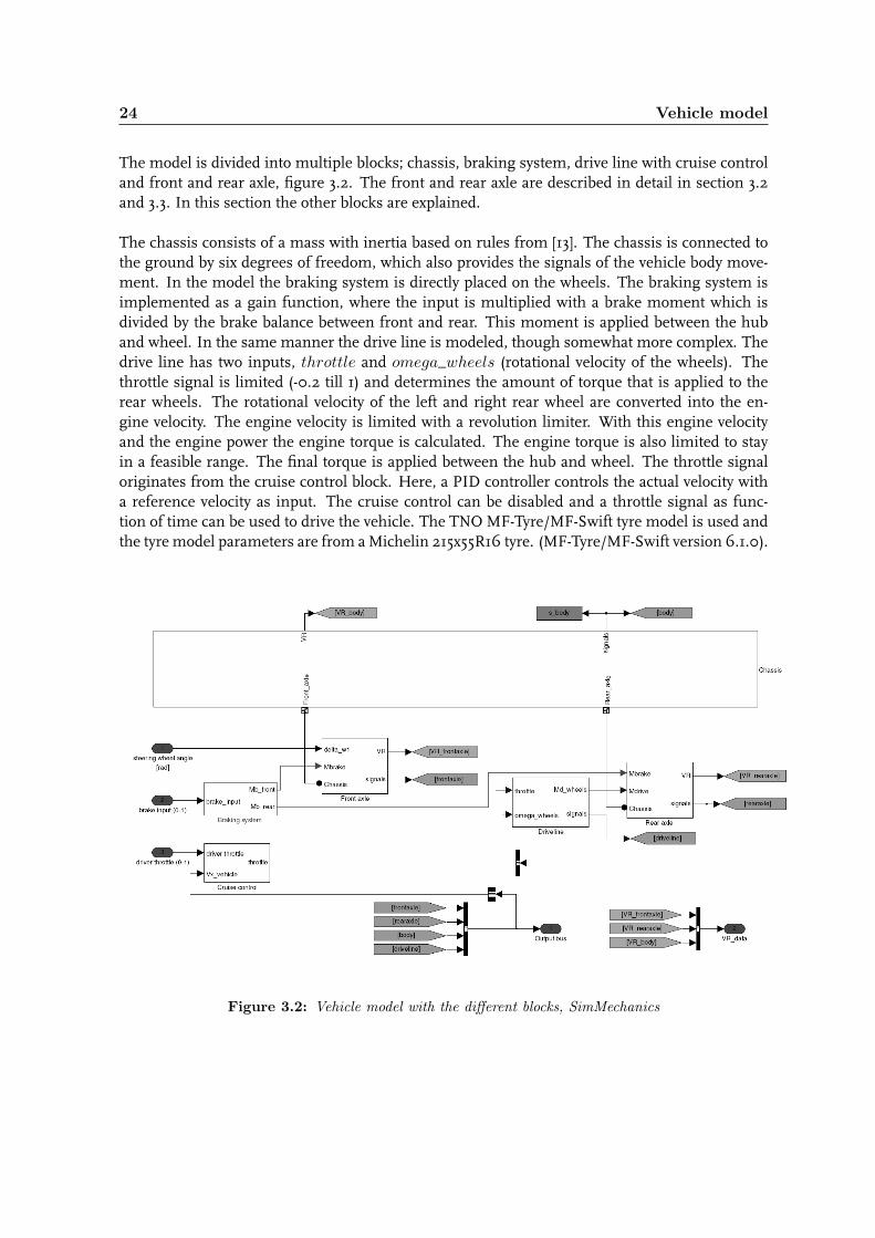
The model is divided into multiple blocks; chassis, braking system, drive line with cruise controland front and rear axle, figure 3.2. The front and rear axle are described in detail in section 3.2and 3.3. In this section the other blocks are explained.

The chassis consists of a mass with inertia based on rules from [13]. The chassis is connected tothe ground by six degrees of freedom, which also provides the signals of the vehicle body move-ment. In the model the braking system is directly placed on the wheels. The braking system isimplemented as a gain function, where the input is multiplied with a brake moment which isdivided by the brake balance between front and rear. This moment is applied between the huband wheel. In the same manner the drive line is modeled, though somewhat more complex. Thedrive line has two inputs, throttle and omega_wheels (rotational velocity of the wheels). Thethrottle signal is limited (-0.2 till 1) and determines the amount of torque that is applied to therear wheels. The rotational velocity of the left and right rear wheel are converted into the en-gine velocity. The engine velocity is limited with a revolution limiter. With this engine velocityand the engine power the engine torque is calculated. The engine torque is also limited to stayin a feasible range. The final torque is applied between the hub and wheel. The throttle signaloriginates from the cruise control block. Here, a PID controller controls the actual velocity witha reference velocity as input. The cruise control can be disabled and a throttle signal as func-tion of time can be used to drive the vehicle. The TNO MF-Tyre/MF-Swift tyre model is used andthe tyre model parameters are from aMichelin 215x55R16 tyre. (MF-Tyre/MF-Swift version 6.1.0).

Figure 3.2: Vehicle model with the different blocks, SimMechanics

3.2 Front axle 25

3.2 Front axle

The front axle of the model is of the McPherson type, see figure 3.3 for a basic layout of this typeof suspension.

Figure 3.3: Basic design of a McPherson suspension, [43]

This type of suspension consists of a lower wishbone (control arm), a spring-damper strut and ahub to which the wheel is connected. An important part of the front axle is the steering systemwhich is also connected to the hub.

3.2.1 Steering system

The steering system used in the BMW 5 series is of the rack and pinion type, an example is shownin figure 3.4.

Figure 3.4: Rack and pinion steering system, including the flexible parts, [44]

The steering wheel is connected by a flexible steering shaft and flexible coupling to the pinion.

26 Vehicle model

The pinion is connected to the rack. When the steering wheel is rotated, the pinion will rotateand translates the rack, the rack is connected to the wheel hub and will rotate the wheels. Thesteering system is modeled on the basis of the following momentum equilibrium, [45]:

Isw · δsw + d(δsw − δp) + c(δsw − δp) = Frack · rp (3.1)

In this equation steering compliance is introduced with the stiffness c, d is the steering dampingand Isw is the steering wheel inertia, Frack is the force with which the rack is actuated and rpis the pinion radius. δsw is the steering wheel angle and δp the angle of the pinion. Steeringcompliance originates from flexible parts in the steering system, as shown in figure 3.4. Theseflexible parts are added to the steering system to filter out vibrations from the road/tyres to thesteering wheel, but also results in a loss of steering angle. This means, some of the input to thesteering system, whether steering wheel or road/tyre input, will be lost due to deformations inthese flexible parts. The effect of implementing compliance can be seen in figure 3.5 where theresponse of the system to a step-input is shown.

Figure 3.5: Steering response of a step-input at 50 km/h

The connections of the steering links to the hub are placed in such a way that Ackerman steeringis introduced. A line is taken from the center of the rear axle to the contact point of the front tyres.The connection of the steering linkage to the hub has to be on this line to achieve Ackermansteering. Ackerman is used to get a difference in steer angle between the outer wheel and innerwheel during cornering. Complete Ackerman steering is usually not feasible, this has to do withpackaging space in wheel bays. In figure 3.6 one can see the effect of Ackerman steering inthe model. The toe-out line corresponds to 50 percent of Ackerman steering. This figure is inagreement with literature, [2].

3.2 Front axle 27

Figure 3.6: Ackerman principle

3.2.2 Suspension model

For the model, the geometry of the McPherson suspension is based on literature, [46], and pic-tures of the vehicle, see appendix A. The basic setup of the front axle can be seen in figure 3.7.

Figure 3.7: Setup of the front axle, left front

For NVH (Noise, Vibration and Harshness) reasons a suspension is equipped with rubber parts,so-called bushings. In the model a bushing is introduced at the front of the lower control arm, seefigure 3.7. The rear connection of the lower control arm to the chassis is connected by a universal

28 Vehicle model

joint. The lower control arm is connected to the hub with a spherical joint, which is also the casefor the connection of the steering linkage to the hub and steering rack. Not shown in figure 3.7is the spring/damper-strut, which is modeled with a prismatic joint. The spring is modeled asa constant stiffness and the damper with a look-up table where the damping force is dependenton the velocity of the joint movement, see figure 3.8. The roll stabilizer is modeled as a stiffnessmultiplied with the difference in the vertical movement of the left and right strut.

Figure 3.8: Front axle damper characteristic, [47]

3.2.3 Kinematics and Compliance

The geometry of a suspension is important for vehicle handling, steering and ride comfort. Kine-matics and compliance (K&C) determine how the suspension geometry changes due to wheelmotions (kinematics) and wheel loads (compliance). Different sources are used to verify the K&Cof the front and rear axle, [2, 48]. K&C tests are performed on a test-rig where the vehicle bodyis attached to a table and the wheels are placed on pads. The movement of the axle is measuredat the wheel center, the forces on the axle are deployed by moving the wheel pads. The followingtests are used to verify the front and rear axle, [49]:

• Bounce: The wheel pads move the vehicle through a sinusoidal vertical motion. During thismotion the wheel pads are controlled to maintain zero force and moments in the horizontalplane, to ensure that the measured displacements are purely kinematic. The bounce test isperformed with locked brakes.

• Roll: The vehicle is put through a roll motion, controlled in such a way that the total load(vehicle force) remains constant. This is to reproduce the kinematics of a vehicle duringcornering. The simulation is performed with a sinusoidal vertical motion as the bouncetest. Only the left and right wheel have an opposing force.

3.2 Front axle 29

• Lateral compliance: The pads perform a lateral motion to generate lateral forces. During thesimulations the forces are both in opposite direction. Equal (but opposite) forces are appliedleft and right to determine the lateral stiffness of the suspension and steering system. Thistest also delivers a lateral compliance steer gradient, which is derived from the measuredtoe-angle. In the simulations, instead of moving the pads, a lateral force is applied at thetyre contact patch. When the forces on one axis are both in opposite direction the steeringsystem stiffness (steering column) will not be included in the results. When the forces arein the same direction and the steering wheel is kept fixed, the steering system stiffness isincluded.

• Longitudinal compliance: Similar to the lateral compliance test but with a longitudinal forceapplied (both wheels symmetrical). Results are the longitudinal suspension complianceand compliance steer.

• Turning compliance: In the contact patch a moment around the z-axis is deployed and thewheel angle is measured. In the simulation the steering wheel is kept fixed, both momentsare in the same direction, this makes that the steering system stiffness is also taken in withthe results.

Some points of attention with respect to the kinematics and compliance tests are, [49]:

• Toe-angle, in principle one wants to keep the toe-angle as small as possible, to preventtyre wear and high lateral forces during jounce. A small toe-change is useful to induceundersteer behaviour. During bounce toe-out on the front axle is desirable.

• Camber change influences the understeer behaviour. For increased lateral grip in corneringnegative camber during jounce is needed.

• Longitudinal; the wheel will move rearwards during jounce and forward during rebound.When driving over a bump, one wants the wheel to move backward. This improves impactharshness (ride). The forces on the suspension are lower compared to the simulation wherethe wheel moves forward, this is preferable for both low as high road load (ride height).

• Lateral displacement at the road contact point. This characteristic equals half the trackchange, track change causes a rolling tyre to slip which introduces lateral forces. Theseforces result in increased rolling resistance. It is desirable to have minimal track change.

• In relation to longitudinal compliance, toe-in during braking and toe-out during driving isa common setup. For the rear axle almost no compliance during braking and driving isdesired.

• Lateral compliance; toe-out for the front axle and toe-in for the rear axle is desired when thewheel is moved inward. This reduces the side slip angle, and generates more understeer.Lateral stiffness needs to be as high as possible to meet vehicle requirements for steeringand handling.

• In reality the vehicle will dive/squat during braking and driving, so toe-angle changes occurthrough jounce, compliance and the static toe-angle.

30 Vehicle model

The model was tuned by hand. First a suspension model was build on the basis of pictures of thesuspension. When the kinematics were comparable with the figures from [2, 48], the model wasmodified to include the compliance. During the tuning process the following assumptions wereused:

• The kinematic toe-angle is mainly dependent on the placement of the steering linkage.Making the steering linkage longer/shorter results in a less/more circular characteristic.The imaginary center of the circular characteristic is determined by the height of the con-nections of the steering linkage (hub and rack) in relation to the placement of the underwishbones, [12]. To achieve the desired toe-changes through compliance, the bushing andsteering system are placed in front of the center of the front axle.

• Camber can be tuned by adjusting the length and placement of the lower control arm (wish-bones).

• The lateral displacement is coupled to the camber angle. The more circular the character-istic (shorter wishbones) the more lateral displacement.

• Longitudinal displacement is mainly determined by the difference in height between thefront and rear connection of the lower control arm to the chassis. Since a backward move-ment during jounce is desired, the front connection of the lower control arm to the chassisis placed a little higher than the rear connection.

• One leg of the lower control arm was at first modeled as a spring to introduce compliance,later on this is replaced by a rod and bushing configuration as this gives better resultsduring the K&C tests. The bushing gives the opportunity to define stiffness and dampingin all six DOF, the damping has an influence on the hysteresis in the K&C characteristics.In the x, y plane the stiffness is determinative in z-direction the spring damper systemcontrol the behaviour therefore, the stiffness in of the bushing in z-direction is relativelystiff. In reality, all connection points to the chassis are mounted in rubber elements, butthis will increase simulation time which is not preferable. Therefore, only one bushing ismodeled.

• Compliance depends on the stiffness used in the bushing and on the layout of the suspen-sion. Since only one bushing is used in the model, the angle of the rod of the lower controlarm connected to this bushing determines (with the stiffness) the ratio between longitudi-nal and lateral compliance. The position of the connection of the steering linkage to thehub in relation to the bushing position largely influences the direction of the toe-changesthat occur during the compliance simulations.

3.2.4 Results

From the final model the following results are obtained. In figure 3.9 the results for the bounceand roll test are visible. The toe-angle is kept within limits.

Also the other results are comparable with data from literature, [2, 49]. In table 3.1, the results ofthe compliance tests are given. When these data are compared with the literature, the values arecomparable with vehicle ten of [48].

3.2 Front axle 31

Figure 3.9: Kinematics and compliance characteristics of the front axle

Table 3.1: Compliance characteristics of the front axleBounce stiffness 24 [N/mm]

Roll stiffness 44 [N/mm]Lateral stiffness 1.40 [kN/mm]

Toe-angle due to lateral force (toe-out) 0.31 [deg/kN]Longitudinal stiffness 0.2 [kN/mm]

Toe-angle due to longitudinal force (toe-out) 0.625 [deg/kN]Steering stiffness, Mz 0.003 [deg/Nm]

32 Vehicle model

3.3 Rear axle

The rear axle of the BMW 5 series is an integral multilink suspension. In figure 3.10, one can seean example of the integral multilink suspension.

Figure 3.10: Integral multilink suspension, BMW 5 series (e39), [46]

The integral suspension in this case consists of a lower arm (wishbone) where one link is con-nected directly to the hub and the other is connected to the hub via the integral link. On top,two rods connect the hub with the chassis, the leading link and rear link. The spring-damperstrut is mounted between these two upper links. In figure 3.11 a schematic representation of theintegral link suspension is shown. An interesting aspect of this axle is the integral link, which isresponsible for the torsional stiff support of braking torques [50].

3.3.1 Modeling

Geometrical data from the rear-axle is not available. Therefore, pictures of the vehicle (appendixA) and papers on this rear axle are used to estimate the dimensions of the rear axle, [46, 50, 51].First a rectangular outlay is chosen, with this suspension a bounce test is performed to obtain thekinematics. Since these kinematics were not good, with each iteration, a single rod is changed toobtain a better result. The targets for the kinematics come from literature [2, 48, 49]. After thekinematics simulations were satisfying, the suspension is modified to test the compliance of theaxle. In figure 3.13, one can see a sketch of the rear axle. Here one can see where the complianceis modeled. A bushing is used (on the front rod of the lower wishbone) and stiffness is added todegrees of freedom of the chassis-connection of the rear link (x-, y-, z-direction) and leading link(only y-direction). Like with the front axle, the spring is modeled as a constant stiffness and forthe damper a look-up table is used, figure 3.12. The assumptions used during tuning are:

3.3 Rear axle 33

Figure 3.11: Model of an integral multilink suspension, [50]

Figure 3.12: Rear axle damper characteristic, [47]

• The longitudinal displacement during bounce is dependent on the angle of the lower wish-bone. The angle determines if the wheel will move rearward during bounce or forward.The length of the rod determines the curvature of the movement.

• Y- and z-position of the leading link on both hub and chassis side have an influence on thecambermovement. The cambermovement is coupled with the lateral displacement. There-fore, one makes a compromise between the camber and lateral displacement motion. Aswith the longitudinal displacement the length of the leading link determines the curvatureof the characteristics.

• The toe-angle during bounce is not depending on a single rod. The whole layout determinesthe toe movement. The toe-angle is coupled to the longitudinal displacement, damperplacement and notably the x-position of all the rods, since these determine toe-out or toe-

34 Vehicle model

in during bounce. Next to that the toe-angle also depends on the stiffness of the differentbushings.

• Without the use of bushings or stiffness the whole rear suspension is infinitely stiff. Firstonly one bushing was modeled but this proved to be insufficient. Since the suspensionexists of three stiff rods additional stiffness is modeled in the form of additional degrees offreedom of the upper links.

• Lateral and longitudinal compliance is tuned with the stiffness of the bushing and thestiffness applied to the additional degrees of freedom. Another point which has influenceon the stiffness is the layout of the suspension. Increasing the angle of the rods moreoutward (x-position on the chassis) gives a stiffer structure. Also the angles of the rods havean influence on the stiffness.

Figure 3.13: Sketch of the rear axle

3.3.2 Results

Similar to the front axle also the rear axle is simulated on the K&C test rig. The kinematics of therear axle are obtained by performing a vertical bounce test. In figure 3.14, one can see the resultsof this test. In the same figure the roll of the axle is depicted.

The compliance of the rear axle is validated by performing tests where longitudinal force, lateralforce and a turning moment are applied at the tyre road contact patch. In table 3.2, the resultsof the compliance tests is given. As with the front axle the characteristics of the rear axle arecomparable with the data from literature, [2, 48, 49].

3.3 Rear axle 35

Figure 3.14: Kinematics and compliance characteristics of the rear axle

Table 3.2: Kinematics and compliance, characteristics of the rear axleBounce 26 [N/mm]

Roll 31 [N/mm]Lateral stiffness 0.82 [kN/mm]

Toe-angle due to lateral force (toe-in) 0.048 [deg/kN]Longitudinal stiffness 0.35 [kN/mm]

Toe-angle due to longitudinal force (toe-in) 0.34 [deg/kN]Steering stiffness, Mz 0.0027 [deg/Nm]

36 Vehicle model

3.4 Four wheel steering

For analyzing four wheel steering, it is important that the model is able to steer with the rearwheels. Because the rear wheel in figure 3.13 can not be steered, the suspension needs to be mod-ified. Therefore, one rod of the multilink suspension is adapted and is equipped with an actuator.The actuator displaces the rod, thus pulling or pushing the wheel. The rod which is used is theleading link. This link is mainly responsible for the toe-angle adjustment during tuning of theK&C settings. In figure 3.15, one can see the adapted rear suspension.

Figure 3.15: Rear axle including actuator

Now that the vehicle is able to steer the rear wheels, the displacement which corresponds withthe steering angle is determined with the K&C model. Here, a static displacement is given to theactuator and this results in a toe-angle, a stroke of 1 [mm] corresponds to a toe-angle angle of ap-proximately 0.38 degrees. The maximum steering angle which is applied is limited to 3.5 degrees(stroke of the actuator, approximately 20 [mm]). This corresponds to steering angles found inliterature, see section 2.4.

Since the suspension is changed, the new model needs to be validated. The rear axle is testedwith K&C simulations to see if there is a change in the behaviour. The actuator has no influenceon the kinematics and compliance of the rear axle. The results of vehicle tests are identical to theoriginal model (lane change, j-turn, braking in a turn).

3.5 Driver model 37

3.5 Driver model

When analyzing a steering system or vehicle steering behaviour, it is important to include driverdynamics. For instance, to include, [5]:

• Dead time resulting from information processing in the central nervous system.

• A delay due to the dynamics of the muscular system.

• Including steering wheel dynamics.

• Predictive action of the driver.

• A gain representing the drivers proportional action.

The system becomes closed loop by including a driver in the model see figure 3.16. An importantfactor is also that a driver will react to deviations from the path, with an open loop simulation thiseffect can not be observed.

Figure 3.16: Open en closed loop

Figure 3.17: Look-ahead driver model, [13]

Figure 3.17, illustrates the driver model which is used in this thesis. A good driver model wasnot available therefore, this basic driver model is used. The model works as follows; first a pathhas to be given on the basis of x, y and z coordinates. Three parameters are measured on the

38 Vehicle model

vehicle model, position of the front- and rear axle in x, y direction and the longitudinal velocity ofthe vehicle. On the basis of the forward velocity and the lookahead time, the length of the vehicleheading vector is calculated. First it is determined which point of the open loop steering trajectory(see figure 3.17) is closest to the model (preview point), then the distance between preview pointand driver path is calculated on the basis of vector projection. The angle ψps is then calculatedbetween these lines and multiplied with the steering ratio and steering sensitivity to arrive at thefinal steering wheel angle. Parameters which can be adjusted are:

• Steering sensitivity: Scaling factor for the final steering angle.

• Number of discrete points: The number of points which are used in the calculation of thedistance between the vectors. The points are a part of the total driver path close to thevehicle. Increasing the number of points will increase calculation time.

• Look-ahead time: Time to calculate the length of the heading vector (also using the vehicleforward velocity).

• Steering ratio: Ratio between steering wheel angle and front wheel angle.

Figure 3.18, shows results from a simulation including the driver model. The simulation is firstperformed with the normal vehicle model (open loop). After that the x, y and z coordinates of thepreview point from this test are used as driver path for the model equipped with the driver model(closed loop).

Figure 3.18: Double lane change test with model with (driver) and without driver model (normal)

As one can see, there is a difference between the two simulations. This is mainly the delay inresponse using the driver model. The driver model steers toward the path, where the normalmodel is already on this path, this causes a delay.

3.6 Full vehicle model validation 39

3.6 Full vehicle model validation

The model including the front and rear axle is build1. In figure 3.19, the virtual reality representa-tion of the model can be seen. To validate the complete model, driving tests have been performed.These tests have been executed according to the ISO standards, [47]. The tests are simulated withthe model of the unloaded vehicle and the results are compared with measurements on the realvehicle.

Figure 3.19: Virtual Reality representation (wheels are not depicted)

3.6.1 Steady state circular test

During this test, the vehicle follows a circular path with a radius of 100 [m] with constant velocity,(ISO 4138). The test is repeated at different velocities giving a velocity-dependent characteristic.With increasing velocities the lateral acceleration will increase, till approximately 8 [m/s2]. In fig-ure 3.20, one can see the final result of the simulation, compared with the measurement. As onecan see, the side slip angle β is somewhat higher than the measurement and the model is slightlymore understeered in comparison to the real vehicle. Overall the model is good in comparisonwith the real vehicle.

Some considerations in relation to simulating the steady state circular test: The steering wheelangle starting point (at low lateral accelerations) is determined by the steering ratio, the curvatureis dependent on the steering and suspension compliance, a stiffer front suspension makes thevehicle less understeered. The side slip angle β is mainly dependent on the rear axle and for alarge part on the lateral compliance toe-angle (rear axle). The roll angle can be influenced by thecenter of gravity. Changing the anti-roll bar stiffness has an influence on both steering behaviourand roll angle of the vehicle body.

3.6.2 Pseudo random steer test

This test is one where a random steering input is generated by the test driver, (ISO 7401). Thegoal of this test is to excite the vehicle and measure the response over the entire frequency rangeof interest, so the transfer functions can be calculated between steering input and response data.The lateral acceleration during the test remains below 4 [m/s2], the boundary below which vehi-cle behaviour can be regarded as being linear. The forward velocity of the vehicle is kept constant

1Model used during validation is without the four wheel steering system, this is tested separately.

40 Vehicle model

at 100 [km/h]. In figure 3.21, one can see the results of the pseudo random steer test, the simula-tion results are quite close to the measurement.

Figure 3.20: Steady state circular test, measurement versus simulation

As with the steady state test, the steering compliance determines the graphs of the steering wheelangle versus lateral acceleration and roll angle, at the lower frequencies. By changing the inertiaof the vehicle on the basis of rules from [13], the simulation results will change. The rules makesure that the inertia’s stay in a feasible range. Mainly, the place of the peaks and dips can betuned in this manner. The whole graph can be shifted horizontally over the x-axis by changingthe inertia around the z-axis, Izz . The peak of the roll angle versus lateral acceleration can bemoved by changing the inertia in x-direction, Ixx. The peaks/dips themselves can be tuned byincreasing/decreasing the damping of the compliance parts which are modeled in the suspensionfront and rear. The vehicle dampers are measured on a test bench and therefore not changed. Theinfluence of the relaxation length is small, influence on roll response is negligible. The influenceon steering response is noticeable, where the phase angle of lateral acceleration to steering wheelangle becomes better with decreasing relaxation length (10 percent), the magnitude peak of yawvelocity response to steering wheel angle becomes better, the phase angle deviates more from themeasurement.


Figure 3.21: Random steer test, unloaded

42 Vehicle model

3.6.3 Loaded vehicle model

An additional validation is performed to see how the loaded model behaves compared to vehicletests. The mass is increased, the center of gravity moves backward and the inertia is adapted.In figure 3.22, one can see the results of the steady state circular test with the loaded vehicle.Steering angle and roll angle are comparable with the measurement, only the side slip angle β istoo high. The side slip angle was already high with the unloaded model, but during the measure-ment the sensor is mounted in the middle of the vehicle, instead of in the center of gravity whereit should be. For the unloaded situation this is not really a problem since the center of gravity isalmost at the center of the vehicle. For the loaded simulation the sensor is placed forward (as inthe measurements) but there is still a deviation.

Figure 3.22: Steady state circular test, loaded situation

In figure 3.23, one can see the results of the random steer test with the loaded model and vehicle.The height of the sensor was not documented. Therefore, this is tuned to give the peaks the rightheight. The inertia is adapted to get a better result from the simulation. Izz is increased to movethe transfer functions of yaw and lateral acceleration to steering wheel angle to the left, next tothat the lateral acceleration peaks increase and yaw peaks decrease. Ixx is changed (lowered) toget the figure of roll angle to lateral acceleration good. The height of the center of gravity hasan effect on the roll angle. The simulation show comparable results. Only in the graph of yawvelocity to steering wheel angle, the simulation gives too high results.


Figure 3.23: Random steer test, loaded situation

44 Vehicle model

3.6.4 Additional tests

The previous tests are performed to validate the model, additional tests are performed to see if themodel is representative for the real vehicle during different maneuvers. The tests are performedwith the unloaded model, the following tests are performed:

• Double lane change (ISO/TR 3888 ): Double lane change is a discrete, closed loop, handlingtest. Closed loop in the sense that the driver has to follow a prescribed path. The simulationis performed with cruise control on, and the steering angle of the measurement is used asinput.

• J-turn (ISO 7401): with the step input, the overshoot in yaw and lateral acceleration, re-sponse time and rise time of lateral acceleration, yaw velocity and roll angle are analyzed.The simulation is performed with cruise control on and the steering angle of the measure-ment is used as input.

• Straight line braking (ISO 6597): with this test the braking behaviour is tested. The dis-tance needed to come to a standstill from an average velocity of 100 [km/h] is an importantparameter in this test. For the simulation, the brake input is tuned to fit the measurement.

• Braking in turn (ISO 7975): This is a complex test and uses almost all relevant parame-ters of the vehicle: mass, geometrical parameters, suspension system, steering system andbraking system etc. Important are the conflicting aims between stability and attainable de-celeration during the braking. Like the straight line braking test, the brake input for thesimulation is tuned in comparison with the measurement (on both the forward velocityand longitudinal deceleration signal).

• Power off (ISO 7975): This test is similar to the braking in a turn test. In this case insteadof braking at a constant lateral acceleration of 4 [m/s2] the throttle pedal is released ona circular path with radius of 100 [m]. Similarly to the braking in a turn test, this testevaluates vehicle stability and predictability in response to the change in longitudinal tireforces. For the simulation, a negative throttle signal is used instead of a brake input.

• Cross wind behaviour (ISO 12021-1): wind speed 18 [m/s], length of wind zone 28.3 [m].Importance of this test is the stability of the vehicle during external disturbances. Duringthe simulation a force is applied to the center of gravity of the chassis. This is different tothe measurement where first the front of the vehicle is influenced by the wind force and inthe end the rear of the vehicle.

Figures 3.24, 3.25, 3.26, 3.27, 3.28 and table 3.3 give the results of the additional tests. As one cansee, the simulation results are comparable with the measurements. Both lane-change and J-turnsimulations are comparable with the measurement, although the model has a faster responsecompared to the measurement. With straight line braking the model comes close to the vehicle,only the deceleration is lower. During the simulation the deceleration is more constant thanduring the measurements. For the braking in turn test, the model shows a similar behaviourcompared to the vehicle test. This is somewhat improved by changing the brake balance more tothe rear, and decrease the brake input. The relaxation effect can be seen when the vehicle comesto a hold. There is a resonance at the end, where without using the relaxation length the signalcomes directly to a hold. With the Power off test the deceleration shows an effect that is different

3.7 Discussion 45

from the measurement. The lower starting point is because the model is cornering which causesthe vehicle to slow down. The accelerations are comparable, both about 1 [m/s2]. An attempt hasbeen made to approximate the effect of the crosswind, but it is clear that this is only a very roughanalysis.

Table 3.3: Straight line brakingparameter measurement simulation

braking distance 43.6 [m] 44.4[m]braking time 3.1 [s] 3.2 [s]

average deceleration 9.36 [m/s2] ≈ 8.4 [m/s2]

3.7 Discussion

The vehicle model is validated on the basis of vehicle tests. The front and rear axle are build on thebasis of their kinematics and compliance characteristics. With these characteristic within feasibleranges, the complete vehicle model is compared with measurements. All vehicle tests show asimilar behaviour between the simulation and measurements. One can conclude that the modelis a accurate representation of the real vehicle. However, the model can be improved by designinga more realistic drive-line including axles or by the introduction of aerodynamics. Aerodynamicscan improve the model behaviour during braking, power off and crosswind tests. A good drivermodel was not available. The driver model should be improved by including both driving andbraking and improve the accuracy of the model. The driver model does not perform good whenapplying constant steer angles, also the deviation from the desired path has to be limited.

46 Vehicle model

Figure 3.24: Double lane change

3.7 Discussion 47

Figure 3.25: J-turn

48 Vehicle model

Figure 3.26: Braking in a turn, brake input is the force on the brake pedal measured during the vehicletest

3.7 Discussion 49

Figure 3.27: Power off

50 Vehicle model

Figure 3.28: Crosswind behaviour

Chapter 4Toe-control

As written in chapter 2 there are different reasons to use active steering on vehicles. In this chap-ter a form of active steering is investigated, known as toe-control. Toe-control is chosen since thiscan be used as addition to compliance characteristics of a vehicle (section 3.2). Next to this alsorecent developments from Hyundai and Prodrive show the potential of toe-control. The effect ofchanging the rear toe-angle is larger than changing the front toe-angle. Therefore, toe-control onthe rear axle is investigated.

In this chapter first section 4.1 is dedicated to asses the desirable toe characteristics and how thiscan be judged. Afterwards, a control strategy is developed to improve the vehicle behaviour. Withthe controller a number of simulations are performed to see how the controlled vehicle model isimproved with respect to the baseline vehicle. Both open loop and closed loop simulations areperformed. Especially during a lane change it is important that a vehicle follows a path, whereaswith a given steer angle (open loop) the vehicle can deviate from the initial path. The modelequipped with toe-control is also compared to alternative rear wheel steering systems. Finally theresults are summarized in a discussion.

4.1 Criteria

In this first section the criteria for an improved vehicle are determined. The baseline vehicle onwhich the improvements will be based is the model from chapter 3. Toe-control is analyzed onthe basis of simulation results, no vehicle tests are performed with a real vehicle. In chapter 3already a rear steering device is described which will be used for toe-control.

A number of representative tests have been selected to evaluate active toe-control. To includeall dynamic features, cornering, braking and straight line stability the following tests are used tojudge toe-control:

• J-turn

• Lane change

• Braking in a turn

52 Toe-control

• µ-split braking test

• Crosswind test

It is difficult to gain an objective criterion to judge improvements in vehicle behaviour. In thefollowing list some possibilities are given:

• Side slip angle β; with an increasing side slip angle the vehicle stability will decrease andthe driver can lose control. Therefore a small side slip angle β is preferable, [52].

• Yaw rate; overshoot in yaw rate is undesirable and can lead to fishtailing, which leads to anincreased workload for the driver, [29].

• Lateral acceleration; a direct response to steer angle inputs. Faster response is effective inimproving handling qualities in a lane change, [5].

• Driver workload; small steering angle is preferred.

• Understeered vehicle is preferred over an oversteered vehicle.

• Tyre utilization; the amount of tyre force (Fx and Fy combined) which is obtained duringdriving in comparison to the maximum tyre force available. Small utilization means onecan utilize the tyres more, and one is further away from the adhesion limits of the tyre(appendix C).

• Delay in yaw velocity and lateral acceleration versus the steering angle, less delay is desir-able.

The items above lead to the following criteria on which improvements will be based. Lowermagnitude of vehicle signals is an improvement, especially a decrease in side slip angle. Anundersteered vehicle, less tyre utilization and a quicker responding vehicle are improvements.Next to these objectives also ideal toe settings are known, recall table 2.1. On the basis of thesetests and objectives a control strategy is developed.

4.2 Control strategy

With toe-control one can actively influence the dynamic behaviour of the vehicle by applying anadditional toe-angle. From literature it is known that the toe-angle setting depends on the sit-uation. First the influence of static toe-angles is analyzed. Simulations are performed with thebaseline vehicle model where the static toe-angle is changed from toe-in to toe-out. From thesesimulations the preferred toe-angle setting for different conditions is obtained, table 4.1. Here themain criterion for an improvement of vehicle handling behaviour was the decrease in magnitudeof the vehicle signals.

When changing the static toe-angle one is basically changing the cornering stiffness. A toe-inangle increases the cornering stiffness. The effect on vehicle dynamics can be demonstrated us-ing the bicycle model, (appendix B). Simulations are performed with the bicycle model. Here thebaseline model, from appendix B, is compared with the bicycle model where the rear corneringstiffness is increased with 20 percent. In figure 4.1 one can see the effect of increasing the rear

4.2 Control strategy 53

Table 4.1: Desirable toe-angle settingssituation front rearcornering toe-out toe-in

accelerating in corner toe-out toe-inbraking in corner toe-out toe-in

external disturbance - toe-indriving straight (braking/driving) none none

cornering stiffness during a step steer test. The magnitudes of the vehicle signals, lateral accel-eration and yaw rate, decrease. In figure 4.2, one can see the results a random steer test. As onecan see, the magnitudes of the vehicle signals decrease as well as the phase lag between yaw rateand lateral acceleration to steering wheel angle.

Figure 4.1: Lateral acceleration and yaw rate response of the bicycle model during a step input test,35 degrees steering wheel angle

Till now only the static toe-angle is changed. This is not preferable. When driving straight aheadan angle of the wheels increases tyre wear. Therefore, a control strategy is made in which thetoe-angle changes when it is preferable.

54 Toe-control

Figure 4.2: Results of random steer test with the bicycle model


4.2.1 Toe-control based on the steering wheel angle

At first a controller is developed on the basis of the steering wheel angle (driver input). In theearly years of research on four wheel steering this was a common signal to determine the rearsteer angle. The controller is a proportional feedforward controller, the steering wheel angle isconverted into a toe-angle of the rear wheels. In figure 4.3, the control scheme is given and informula 4.1, one can see the control expression. Here, δr is the toe-angle, Kp is the proportionalgain, x is the vehicle signal (in this case steering wheel angle, δsw) and sat is the saturationcriterion. In the control strategy the toe-angle is limited (saturation) to 3.5 degrees, formula 4.2,this is comparable with maximum steer angles on the rear axle found in literature ([33, 35]). Thetoe-angle is converted into a stroke of the actuator with gain c (a ratio of 0.0026).

Figure 4.3: Control scheme of the proportional controller

δr = sat(Kp · |x|) (4.1)

sat(Kp · |x|) ={Kp · |x| if Kp · |x| < 3.53.5 if Kp · |x| ≥ 3.5

(4.2)

In table 4.2, Kp is given. The proportional gain is based on simulations and literature, [30],where the rear steer angle is approximately 50 percent of the front steer angle. In this case thetoe-angle is around 40 percent of the front wheel steer angle1. With the controller simulationsare performed to see the influence of toe-control.

Table 4.2: Proportional gain, based on the steering wheel anglex Kp

δsw [deg] 0.02052

In figure 4.4a, one can see the effect of the controller during a step test. The simulation isperformed with a steering wheel angle of 35 degrees, the corresponding toe-angle is around 0.7degrees. Both lateral acceleration and yaw rate decrease in magnitude. However, the decreasein the side slip angle is the main advantage. The same test is performed with the driver modelincluded, figure 4.4b. The results with the driver model are comparable with the simulationwithout the driver model. One can see that the real effect of rear toe-control is reducing theside slip angle. The main difference between open- and closed loop is that the open loop modelresponds faster, overall the signals are comparable.

1Because of tuning of the gain, to compare different controllers, the steer angle is not identical to the angleused in literature

56 Toe-control

(a) Without driver model (b) Including driver model

Figure 4.4: J-turn simulation based on control with the steering wheel angle


Table 4.3: Comparison between control on different signalssituation ay δsw r

magnitude ± + −response time + ± −

overshoot − ± +settling time − ± +

4.2.2 Toe-control based on other signals

As one can see in the previous subsection, the toe-controller on the basis of the steering wheel an-gle works and vehicle behaviour is improved. The problem is that this only works when a steeringangle is applied. For instance, when braking or during external disturbances the controller willhave no influence. Therefore, other signals are used as an input for the controller. The followingsignals are used:

• Longitudinal acceleration, ax

• Lateral acceleration, ay

• Yaw rate, r

These signals are chosen since they are relatively easy to measure. Sensors which can measurethese signals are available. For example, the vehicle side slip angle β is difficult to obtain (it re-quires an estimator). Longitudinal acceleration will occur during braking and driving. Especiallyduring braking this signal has advantages. During braking the other signals will decrease (de-creasing forward vehicle velocity) where the longitudinal acceleration will remain constant, tillthe forward velocity becomes zero.

The other two signals, yaw rate and lateral acceleration, are comparable with the steering wheelangle. Both occur during cornering. The lateral acceleration and yaw rate also occur during ex-ternal disturbances. Here the steering wheel angle has no influence. In table 4.3, an overviewis given of the (dis)advantages of using these signals for toe-control. The results are based onsimulations with the different control strategies. As with the controller based on the steeringwheel angle, the vehicle signals are measured during simulation and multiplied with a propor-tional gain, formula 4.1 and table 4.4. The toe-angle is converted into a stroke of the actuator. Theproportional gains are a compromise regarding the following considerations:

• The maximum vehicle signals occurred during the vehicle tests (chapter 3), lead to thevalues where the the maximum toe-angle of 3.5 degrees will be reached.

• When the vehicle is maneuvering and the magnitudes of the vehicle signals is small thecontroller should also work.

• The different controllers should be comparable, the gains are tuned to give approximatelythe same toe-angle during the same vehicle tests.

58 Toe-control

(a) Based on yaw rate (b) Based on lateral acceleration

Figure 4.5: J-turn simulations, baseline vehicle compared to controlled vehicle

Table 4.4: Proportional gain, based on the yaw rate and the lateral and longitudinal accelerationx Kp

r [deg/sec] 0.0977ay [m/s2] 0.35ax [m/s2] 0.2

In figure 4.5 and 4.6, simulations of the control strategy based on the yaw rate and lateral accel-eration are shown. To get a fair comparison between the different controllers, the proportionalgains are tuned to get the same toe-angle as with the controller based on the steering wheel angle.Thus, the results of the simulations between the different controllers are comparable since theyhave the same steer angle, the difference between the controllers depends on the form of thesignals. As one can see in the simulations of the J-turn, control based on the lateral accelerationis faster but it has a longer settling time and the overshoot is higher when compared to controlbased on the yaw rate. Overall the steady state values are approximately the same. The lanechange simulation is performed with driver model (closed loop). In the results of the lane changesimulation the differences are larger, especially at the last steer input where the reaction of thecontrolled vehicle is faster. In the next section the results are combined and one final controlleris made.


(a) Based on yaw rate (b) Based on lateral acceleration

Figure 4.6: Lane change simulations, baseline vehicle compared to controlled vehicle (closed loop)

60 Toe-control

4.2.3 Final strategy

With the knowledge obtained on toe-control the following controller is designed, figure 4.7. Thecontroller is based on vehicle signals to determine the condition of the vehicle, whether it issteering, driving or braking. When the condition is known the signals are used as control inputto improve vehicle handling behaviour.

Figure 4.7: Control strategy

To include all situations the choice is made to use two signals, yaw rate and longitudinal acceler-ation. It is preferable to use yaw rate over lateral acceleration, since is it has less overshoot anda shorter settling time. Although the yaw rate is less responsive than the steering wheel angle, itis chosen since it also works when disturbances act on the vehicle. Longitudinal acceleration ischosen since this gives a clear indication of the behaviour of the vehicle in longitudinal direction.Next to that a third factor is used in the control strategy, the forward velocity of the vehicle. Thisis done since the effect of toe-control is not preferable at low velocity. At low velocity one wantsthe whole rear axle to steer opposite to the front to improve maneuverability. Therefore, below40 [km/h] the controller is disabled. In the block Gain, formula 4.3 is used with the conditionsgiven in formula 4.4, from 40 [km/h] till 60 [km/h], the output is increased from zero to one.

GainVx = sat(0.05 ∗ (Vx − 40)) (4.3)

sat(0.05 ∗ (Vx − 40)) =

0 if V x ≤ 40(0.05 ∗ (Vx − 40)) if V x > 401 if V x ≥ 60

(4.4)

The control law is given in formula 4.5. In table 4.5 the gains Kp1 and Kp2 are given. The toe-angle is limited, see formula 4.6 for the saturation conditions. The controller is a combinationof longitudinal acceleration and yaw rate. For both steering (left/right) and braking/traction toe-in is the preferred setting. Therefore, the absolute values of the vehicle signals are taken. Thegains and limits of the controller are based on simulations with the controlled model. Fromsimulations using a controller based on the longitudinal acceleration the toe-angle during brakingis tuned. The maximum toe-angle when decelerating is two degrees. When the toe-angle is largeror smaller the vehicle signals during braking in a turn deviate from the desired values. The valuesfor the yaw rate are chosen as described in subsection 4.2.2. As one can see during cornering,

4.3 Results of the final strategy 61

with an increasing yaw rate, the toe-angle increases till the maximum of 3.5 degrees. In the nextsection the simulation results of the model with controller are compared to the baseline vehicle.

δr = sat(Kp1 · |ax|+Kp2 · |r|) (4.5)

sat(Kp1 · |ax|+Kp2 · |r|) =

(Kp1 · |ax|+Kp2 · |r|) if ax ≤ 102 if |ax| > 100 if |r| ≤ 1(Kp1 · |ax|+Kp2 · |r|) if r ≤ 303.5 if |r| > 303.5 if (Kp1 · |ax|+Kp2 · |r|) ≥ 3.5

(4.6)

Table 4.5: Proportional gain, longitudinal acceleration and yaw rateKp1 0.2Kp2 0.0977

4.3 Results of the final strategy

The model equipped with the controller is compared to the baseline model from chapter 3. Firstsimulation that is analyzed is the J-turn test. During the test the rear steer angle is approximately0.7 degrees, which is around 40 percent of the front steer angle. In figure 4.8, the results areshown in the form of the vehicle signals. Toe-control improves the behaviour of the vehicle, sig-nal magnitudes decrease. In figure 4.9, one can see the tyre utilization of the model, (appendixC). On the front tyres a small change is visible, on the rear tyres a larger change is visible. Theleft tyre (inside) is less used while the utilization is increased on the right rear tyre (outside). Thisis because of the increase in side slip angle on the right rear tyre, which increases the lateral force.

In figure 4.10 the lane change simulation is shown. The lane change simulation is performedincluding the driver model, closed loop. The side slip angle is decreased, also the other vehi-cle signals are slightly lower compared to the baseline vehicle. The rear steering wheel angle isaround two degrees, which is around 40 percent of the front steer angle. The tyre utilization iscomparable with the j-turn simulation. Utilization of the front tyres is unchanged and on the rearaxle the tyre on the inside is less used and the tyre on the outside is used more.

With the braking in a turn test the controller is used on both longitudinal acceleration and yawrate. In figure 4.11, one can see the results. Because the controller also acts on the yaw ratea small difference between the signals is already visible before the braking begins. From fourseconds the vehicle is braking and till 6.5 seconds the controller is applying a toe-angle. Afterthis the velocity is decreased to below 40 [km/h]. The rear toe-angle is approximately 1.5 degrees.During the first period the benefit of control is clearly visible. Instead of increasing, the signalsdecrease to zero. This behaviour results in an increase of the corner radius which is safer thenwhen the corner radius becomes smaller. A decrease in corner radius can lead to an increase inworkload for the driver. In figure 4.11 also reference data is plotted for lateral acceleration and

62 Toe-control

Figure 4.8: J-turn, vehicle signals, step input of 35 degrees steering wheel angle

Figure 4.9: J-turn, tyre utilization, step input of 35 degrees steering wheel angle

yaw rate. For lateral acceleration the controlled model is close to the reference value. The yaw ratedeviates from the reference value, although the sign is in the right direction. In figure 4.12, thetyre utilization is plotted. As with the other two tests toe-control does not have a large influenceon the front tyres. On the rear tyres more differences are visible. The utilization is more constantwith the controlled model, also the faster response of the controlled model can be seen.


Figure 4.10: Lane change, vehicle signals, maximum steer angle is approximately 60 degrees (closedloop)

Figure 4.11: Braking in a turn, vehicle signals

The following tests are done to see how the model reacts to disturbances, crosswind test and µ-split braking test. As can be seen in figure 4.13, no differences occur during the crosswind tests,only at the peak values small differences are visible. During the crosswind test the disturbance isnot large enough to create a large yaw rate.

64 Toe-control

Figure 4.12: Braking in a turn, tyre utilization

Figure 4.13: Crosswind test, vehicle signals

During µ-split braking toe-control does improve the behaviour of the vehicle, figure 4.14. Inthe same manner as with the braking in a turn test the vehicle signals are decreased. Creatingundersteer instead of oversteer so that the vehicle becomes more stable.


Figure 4.14: µ-split braking, vehicle signals

66 Toe-control

4.4 Alternatives for toe-control

In this section the results from toe-control are compared with individual toe-control and fourwheel steering (4WS).

4.4.1 Individual wheel steering

Besides toe-control on the rear axle, one can also perform control on each wheel individually. Herethe control strategy from the previous section is used and applied individually to the rear wheels.As can be seen in the tyre utilization plots (figure 4.9, rear left tyre) the inner rear wheel has alarge decrease in utilization. The point of using four wheels steering is to reduce the negativelateral force of the rear tyres during turn-in. With toe-control the inner wheel is only increasingthe negative lateral force. When steering only the outer wheel the decrease in tyre utilization isless, though the utilization on the outer wheel remains approximately the same. Therefore, in acorner only the outer wheel is actuated. The outer wheel is detected by the vehicle signals. Lateralacceleration, steering wheel angle and yaw rate can be used. In this case the steering wheel angleis chosen since the chosen simulations use the steering wheel angle as an input. When the steer-ing wheel angle is positive the vehicle is steered to the left and otherwise to the right. Since thecontrol strategy is the same as with toe-control, both controllers have the same gain, only with in-dividual steering one wheel is actuated. In figure 4.15, one can see the results of the comparisonbetween toe-control and individual toe-control. During toe-control the wheel is steered oppositeto the outer wheel and now the inner wheel is kept straight, it is visible that keeping the wheelstraight has an advantage over applying a toe-angle.

4.4.2 Four wheel steering

Four wheel steering mainly consists of normal front wheel steering with the addition that the rearwheels are able to steer. Based on literature [33, 53], a proportional control strategy is developedfor four wheel steering. On the basis of the forward velocity the steer angle ratio between thefront and rear steer angle is changed. The steering ratio is determined in the same manner as informula 2.1. At low velocity in opposite direction and from approximately 40 [km/h] the wheelssteer in the same direction as the front ones. In figure 4.16, the ratio is shown as a function ofthe forward velocity. The main difference between toe-control and four wheel steering is that withfour wheel steering both wheels are steered in one direction. The advantage is that the negativelateral force of the inner wheel on turn in will decrease.

In figure 4.17 the result of a j-turn and lane change simulation are shown. During the J-turnsimulation the steer angle of the four wheel steering controller is the same as toe-control. Whenusing the driver model to stay on a desired path the differences between toe-control and fourwheel steering decrease. With a equal steer angle four wheel steering has more effect on reduc-ing the sideslip angle then toe-control. The response of four wheel steering is slower especiallyduring the lane change, that is because with toe-control the inner wheel is ready to steer to theother direction.

4.4 Alternatives for toe-control 67

(a) J-turn (b) Lane change (closed loop)

Figure 4.15: Comparison between individual steering and toe-control

Figure 4.16: Steering ratio versus forward velocity, four wheel steering

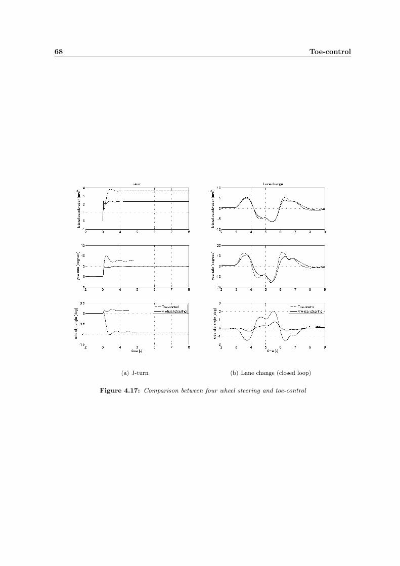
68 Toe-control

(a) J-turn (b) Lane change (closed loop)

Figure 4.17: Comparison between four wheel steering and toe-control

4.5 Discussion 69

4.5 Discussion

The difficulty of improving vehicle handling behaviour is the criterion on which an improvementis based. These criteria should be objective and possible to be measured. The main reason isthat the main objective of this research is to see how toe-control can improve vehicle behaviour.Therefore, the control strategy is kept simple with a proportional controller. The final controlstrategy consists of two signals, the longitudinal acceleration seems to work good during brakingin maneuvers. The other signal, yaw rate, maybe arguable since the effect of the controller dur-ing disturbances is not noticeable, and during steering maneuvers the results do not differ muchfrom the other signals, lateral acceleration and the steering wheel angle.

When on the basis of the criteria the controlled model is compared to the baseline vehicle, onecan conclude that vehicle behaviour is improved. During the steering maneuvers the magnitudeof the vehicle signals is decreased, especially the side slip angle. The vehicle response is quickerespecially when changing from one direction to another (lane change). Since the side slip angleis reduced the model becomes more understeered which is preferable over an oversteering ve-hicle. When looking to the tyre utilization one can argue if this is an improvement, the outsiderear tyre is more utilized and the inside tyre less. Because of applying an additional angle to theouter rear wheel the lateral force increases therefore, the utilization increases. Increasing the tyreutilization increases tyre wear. During extreme situations, braking in a turn, the maximum tyreforce of the front wheels is reached. Because handling behaviour is improved the increased tyreutilization is not a problem.

When comparing toe-control to its alternatives one can conclude that individual steering and fourwheel steering both have their advantages. When comparing the controllers, the initial reactionof four wheel steering is faster and during the j-turn the vehicle signals are lower in magnitude.The real advantage of toe-control is that when the vehicle is steered from one direction to theother, the inner wheel is ready to steer in the right direction, while four wheel steering is slower.Individual steering behaves between these two steering strategies.

An important point is that the results are based on simulations. For accurate conclusions on toe-control one should perform real-life vehicle tests, because with the steering systems the driverfeel is important.

70 Toe-control

Chapter 5Conclusions and Recommendations

The goal of the research was to find the advantages of individual wheel steering in comparison toa conventional steering system, with the main attention to the dynamic behaviour of the vehicle.One can think of the following conditions: step steer test, braking (µ-split or in a corner) or cross-wind disturbances. With this in mind a vehicle model is build which is validated. The validatedmodel performed as baseline model. On the rear axle of the vehicle model a steering actuator ismodeled to make it possible to steer the rear wheels. Criteria is determined on which improve-ments in vehicle handling behaviour will be based. A control strategy is developed on the basis ofvehicle signals. The final control strategy consists of a proportional feedforward controller. In thenext sections conclusions and recommendations are formulated for the two main parts, vehiclemodel and toe-control.

5.1 Vehicle model

From the results of the kinematic and compliance and vehicle tests, one can conclude that themodel is a accurate representation of the real vehicle. In the following summations some conclu-sions and recommendations are given.

Conclusions

• The results from the kinematic and compliance tests show that the front and rear axlebehave within realistic ranges.

• From the steady state test, one can conclude that the model is slightly more understeeredat higher lateral accelerations, and the vehicle side slip angle β is slightly higher than thereal vehicle for the unloaded simulation.

• The results from the random steer test are good, although at higher frequencies the simu-lation deviates from the measurement.

• For the loaded situation the steady state simulation shows some deviations, especially forthe vehicle side slip angle. The Random steer test is comparable with the measurements.

72 Conclusions and Recommendations

Although, here also deviations are present. One of the factors making a comparison diffi-cult, between the loaded vehicle and the model, is that the locations of sensors on the testvehicle are not exactly known.

• The additional full vehicle handling tests show a similar behaviour between the model andthe vehicle.

Recommendations

• A general recommendation is, when one is making a model with this level of detail in thesuspension system it is advisable to have all the (exact) data from the vehicle or have thereal vehicle present. In this way parameters can be measured instead of estimated. For thisvehicle model, the tuning started with kinematics, and after that the compliance was tuned.It is advisable to first collect all the data and then tune the model, for both kinematics andcompliance, since all parameters in some way influence each other.

• The model can be improved by designing a more realistic drive-line including axles or bythe introduction of aerodynamics. Aerodynamics can improve the model behaviour duringbraking, power off and crosswind tests. Power steering can be added to the steering systemmodel when this is desired.

• The driver model used can be improved, for instance by including driving and braking.Next to that the accuracy of the driver model can be improved, limiting the deviation fromthe desired vehicle path and improve the driver behaviour when when applying constantsteer angles.

5.2 Toe-control

From literature, it is known that the toe-angle of a vehicle is important since this can improvecornering behaviour. The toe-angle can be used when braking, in the form of bushings whichallow the wheels to steer during braking. When the toe-angle is actively controlled it can improvevehicle handling behaviour in all situations. This and recent research (Hyundai, Prodrive) led tothe decision to develop an active toe-control system. In the following summations conclusionsand recommendations on the developed active toe-control system are given:

Conclusions

• From literature it is known that the geometry of the suspension is a compromise settingthat has to work in different situations. When designing an active control system thiscompromise is no longer necessary.

• Rear wheel steering has advantages, reduction of the phase delay for the lateral accelera-tion and yaw response, reduction of the side slip angle β, improve stability and improvemaneuverability at low velocity.

• There are advantages for using active steering over other systems. For example steeringrequires less force from the tyre compared to braking. Also no delay is involved and thecomfort is better. The yaw torque which can be generated with steering is higher than othersystems, like braking or torque vectoring.

5.2 Toe-control 73

• Toe-control improves vehicle behaviour. During different vehicle handling tests, the mag-nitudes of vehicle signals decrease significantly. The response of the vehicle on steeringinputs is quicker, especially when steering from one side to another (lane change).

• When toe-control is compared with alternatives, four wheel steering and individual steer-ing, the response of toe-control system is faster then both alternatives.

Recommendations

• Toe-control is now based on simulations but it is interesting is to see how toe-control worksin real-life situations mounted on a vehicle. It is also important to fine-tune the controller(gains) in these situations.

• Since the goal was not to design an advanced controller, the controller used is a relativesimple proportional controller. One can further improve vehicle handling behaviour bydesigning a more advanced controller.

• From the comparison between toe-control and alternatives, it could be interesting to domore research into individual toe-control.

74 Conclusions and Recommendations

Appendices

Appendix AVehicle model

A.1 Parameters

In table A.1, the parameters of the model are given.

Table A.1: Global vehicle parametersVehicle parameters BMW, 1996, 523iGross vehicle weight 1495 [kg]Max. vehicle weight 1955 [kg]

L x W x H 4.775 x 1.800 x 1.435 [m]Wheelbase 2.830 [m]

Track front/rear 1.516 / 1.530 [m]Engine 2.5 liter, 6 Cylinder

Max Power 125 [kW] at 5500 [rev/min]Max Torque 245 [Nm] at 3950 [rev/min]steer ratio 18.3 [-]

78 Vehicle model

A.2 Pictures of the vehicle

Photo’s of the front and rear axle.

Figure A.1: Photo of the front axle (e39), left side front of the vehicle (Driving direction is to theleft)

Figure A.2: Photo of the rear axle, side view, (e60)

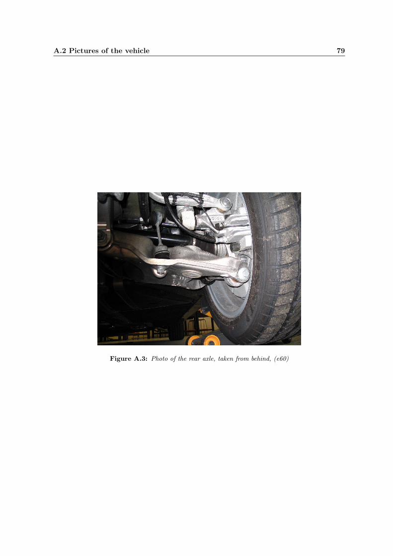
A.2 Pictures of the vehicle 79

Figure A.3: Photo of the rear axle, taken from behind, (e60)

80 Vehicle model

Appendix BBicycle model

In chapter 4 is referred to a bicycle model, figure B.1. In this appendix the equations of motionare given, [29]:

Figure B.1: Bicycle model, [13]

m(v + ur) = Fy1 + Fy2 (B.1)

Izz r = aFy1 − bFy2 (B.2)

Wherem equals the mass of the vehicle, Izz is the yaw moment of inertia, u the forward velocity,v the lateral velocity and r the yaw rate. The lateral force is given by:

Fyi = CFα,iα′i (B.3)

82 Bicycle model

CFα,i represents the tyre cornering stiffness, the index i refer to front and rear tyre. The dy-namic tyre side slip angle α′ is calculated using the following differential equations, includingthe relaxation length σ and the steering compliance c:

σ1

uα′

1 + α′1 = δ1− v + ar

u− CFα,1α

′1c1 (B.4)

σ2

uα′

2 + α′2 = δ2− v − br

u− CFα,2α

′2c2 (B.5)

In table B.1 the values of the vehicle parameters are given.

Table B.1: Vehicle parametersvehicle parameter symbol value

vehicle mass m 1659 kgyaw moment of inertia Izz 2259 kgm2

wheelbase l 2.83 mdistance CG to front a 1.42 m

cornering stiffness front CFα,1 3030 N/deg (2 tyres)cornering stiffness rear CFα,2 3038 N/deg (2 tyres)relaxation length front σ1 0.45 mrelaxation length rear σ2 0.45 m

steering compliance front c1 0.35 deg/kNsteering compliance rear c2 0.05 deg/kN

steering ratio is 19.2

Appendix CTyre utilization

Tyre utilization is the amount of force the tyre uses in comparison to themaximal force obtainablewith a tyre at a specific vertical force. This can be shown in the friction ellips, figure C.1. Whencalculating the tyre utilization the forces from the tyre model are used, Fx, Fy, Fz . With theabsolute values of Fx and Fy the angle ϕ and length of the force in the x-, y-plane are calculated:

ϕ = arctan(Fy

Fx) (C.1)

length =√F 2

x + F 2y (C.2)

To calculate the utilization the maximum force is needed. The maximum force is µFz . Thefriction coefficient is different for longitudinal and lateral force. In figure C.2, one can see thefriction coefficient versus the vertical force. The data for the friction coefficient originates fromthe tyre property file of the tyre. As one can see the friction coefficient decreases with increasingvertical force. The lateral friction coefficient has a steeper decline than the longitudinal frictioncoefficient. With the friction coefficient known the maximum force is calculated:

Fx,max = µx · Fz (C.3)

Fy,max = µy · Fz (C.4)

An ellipse can be described by:

(x

a)2 + (

y

b)2 = 1 (C.5)

Here a is the semi-major axis and b is the semi-minor axis. If a = b, the ellipse is a circle centeredat the origin with radius a. Using the polar coordinates:

x = a · cos(ϕ) (C.6)

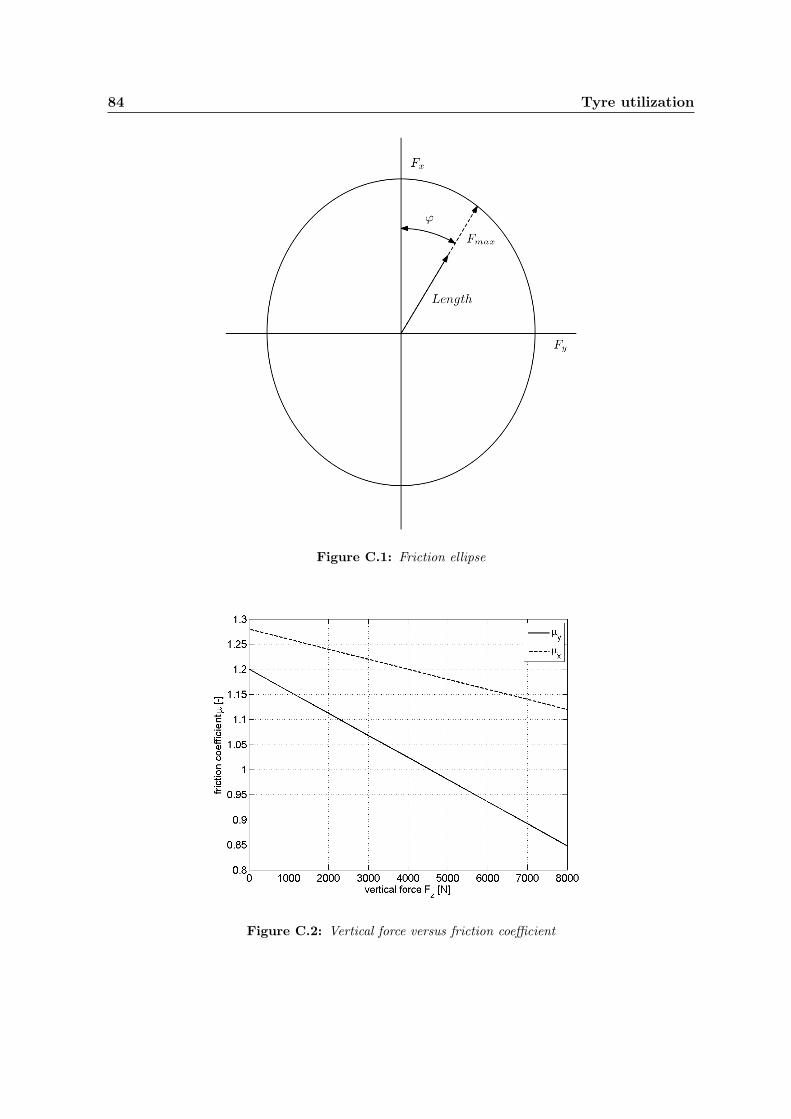
84 Tyre utilization

Figure C.1: Friction ellipse

Figure C.2: Vertical force versus friction coefficient

85

y = b · sin(ϕ) (C.7)

The radius of the ellipse is given by:

Fmax =ab√

b2cos2(ϕ) + a2sin2(ϕ)(C.8)

This maximum force is compared with the force (length) from equation C.2. The percentageused from the maximum force is then calculated:

percentage = (length

Fmax) ∗ 100 (C.9)

86 Tyre utilization

Bibliography

[1] M. Blundell and D. Harty, Multibody systems approach to vehicle dynamics. Amsterdam : Else-vier Butterworth Heinemann, 2004. ISBN: 0-7506-5112-1.

[2] J. Reimpell, H. stoll, and J. W. Betzler, The Automotive Chassis: Engineering principles. Oxford: Butterworth Heinemann, second ed., 2001. ISBN: 0 7506 5054 0.

[3] S. Loth, “Fahrdynamische einflussgrössen beim geradeauslauf van pkw,” Master’s thesis,Technischen Universität Braunschweig, 1997.

[4] R. P. King, D. A. Crolla, and H. A. S. Ash, “Identification of subjective-objective vehiclehandling links using neural networks for the foresight vehicle,” SAE paper, no. 2002-01-1126, 2002.

[5] S. Horiuchi and N. Yuhara, “An analytical approach to the prediction of handling qualitiesof vehicles with advanced steering control system using multi-input driver model,” Journalof Dynamic Systems, Measurement and Control, vol. 122, pp. 490–497, 2000.

[6] D. H. Weir and D. T. McRuer, “Dynamics of driver vehicle steering control,” Automatica,vol. 6, pp. 87 –98, 1970.

[7] D. H. Weir and R. J. Dimarco, “Correlation and evaluation of driver/vehicle directional han-dling data,” SAE paper, no. 780010, 1978.

[8] R. Schindlmaister, J. Dietz, P. Kainz, and T. Kriegel, “The Chassis Concept of the AUDI A5From Ideas to Realisation,” VDI-Berichte, no. 2014, pp. 401–430, 2007.

[9] H.-H. Breass and U. Seiffert, Vieweg Handbuch Kraffahrzeugtechnik. Braun-schwieg/Wiesbaden: Vieweg & Sohn Verlagsgesellschaft mbH, Germany, second ed.,2001. ISBN: 3-526-13114-4.

[10] W. Matschinsky, Road Vehicle Suspensions. St Edmundsbury Press Limited, Suffolk, UK,first ed., 2000. ISBN: 1 86058 202 8.

[11] T. D. Gillespie, Fundamentals of Vehicle Dynmaics. Society of Automotive Engineers, Inc,Warrendale, US, 1992. ISBN: 1-56091-199-9.

[12] W. F. Milliken, D. L. Milliken, and L. D. Metz, Race car vehicle dynamics. Warrendale : SAEInternational, 1995-1998. ISBN: 1-56091-526-9.

88 BIBLIOGRAPHY

[13] I. J. M. Besselink, “Vehicle dynamics.” Lecture notes, 2005. Eindhoven University of Tech-nology.

[14] W. Lamers, “Development and analysis of a multi-link suspension for racing applications,”dct 2008.077, Eindhoven University of Technology, 2008.

[15] M. Y. Rupp, “Passive dynamic steering system model for use in vehicle dynamics simula-tion,” Master’s thesis, Ohio State University, 1994.

[16] N. Irie and J. Kuroki, “4WS Technology and the Prospects for Improvement of Vehicle Dy-namics,” SAE, no. 901167, pp. –, 1990.

[17] Y. Furukawa, N. Yuhara, S. Sano, H. Takeda, and Y. Matsushita, “A Review of Four-WheelSteering Studies from the Viewpoint of Vehicle Danamics and Control,” Vehical Systems Dy-namics, vol. 18, pp. –, 1989.

[18] Y. Shibahata, “Progress and future of chassis control technology,” Annual Reviews in Control,vol. 29, 2005.

[19] J. Ackermann and T. Bünte, “Automatic car steering control bridges over the driver reactiontime,” 1995. DLR.

[20] J. Ackermann, T. Bünte, W. Sienel, H. Jeebe, and K. Naab, “Driving safety by robust steeringcontrol,” 1996. DLR.

[21] J. Ackermann, “Active steering for better safety, handling and comfort,” 1998. DLR.

[22] R. Marino, S. Scalzi, and F. Cinili, “Nonlinear PI front and rear steering control in four wheelsteering vehicles,” International Journal of Vehicle Mechanics and Mobility, vol. 45, no. 12,2007.

[23] J. Ackermann, “Robust Decoupling, Ideal Steering Dynamics and Stabilization of 4WSCars,” Automatica, vol. 30, no. 11, pp. 1761–1768, 1994.

[24] W. J. Manning and D. A. Crolla, “A review of yaw rate and sideslip controllers for passengervehicles,” Transactions of the Institute of Measurement and Control, vol. 29, pp. 117–135, 2007.

[25] J. Ackermann and T. Bünte, “Handling improvement of robust car steering,” 1998. DLR.

[26] J. Ackermann and T. Bünte, “Automatic car steering control bridges over the driver reactiontime,” 1996. DLR.

[27] J. Ackermann, “Robust car steering by yaw rate control,” Proceedings of the 29th conference onDecision and Control, pp. 2033–2034, 1990.

[28] S. Kleine and J. L. V. Niekerk, “Modelling and control of a steer-by-wire vehicle,” InternationalJournal of Vehicle Mechanics and Mobility, vol. 29, pp. 114–142, 1998.

[29] I. Besselink, T. Veldhuizen, and H. Nijmeijer, “Improving yaw dynamics by feedforward rearwheel steering,” 2008. Eindhoven University of Technology.

[30] S.-H. Lee, U.-K. Lee, S.-K. Ha, and C.-S. Han, “Four-wheel independent steering (4wis) sys-tem for vehicle handling improvement by active rear toe control,” JSME International journal,vol. 42, no. 4, pp. 947–956, 1999.

BIBLIOGRAPHY 89

[31] S. H. Lee, H. Sung, J. W. Kim, and U. K. Lee, “Enhancement of vehicle stability by activegeometry control suspension system,” International Journal of Automotive Technology, vol. 7,no. 3, pp. 303–307, 2006.

[32] Renault, “Renault lagune gt, intense pleasure and absolute efficacy.” internet, press release,march 2008.

[33] “Renault steers laguna upmarket,” Automotive Engineer, p. 53, October 2007.

[34] W. Klier, G. Reimann, and W. Reinelt, “Concept and functionality of the active front steeringsystem,” SAE international, no. 2004-21-0073, 2003.

[35] H. Hemmes, “Bmw 7 series offers new styling, lots of in-novation.” http://www.washingtontimes.com/news/2008/aug/01/bmw-7-series-offers-new-styling-lots-of-innovation/, August 2008.

[36] http://www.ae-plus.com/Carcompanies/BMWpics/BMW-7-Series--pic-rear-axle.jpg.

[37] J. Ackermann, T. Bünte, and D. Odenthal, “Advantages of active steering for vehicle dynam-ics control,” 1998. DLR.

[38] B. A. Güvenç, T. Bünte, D. Odenthal, and L. Güvenç, “Robust two degree-of-freedom vehiclesteering controller design,” IEEE Transactions on Control Systems Technology, vol. 12, no. 4,pp. 627–636, 2004.

[39] Y. Furukawa and M. Abe, “Advanced chassis control systems for vehicle handling and activesafety,” Vehicle System Dynamics, vol. 28, pp. 59–86, 1997.

[40] M. Schiebahn, P. W. A. Zegelaar, and O. Hofmann, “Yaw torque control for vehicle dynamicssystems,” VDI-Berichte, no. 2014, pp. 101–119, 2007.

[41] W. Kober and F. Ramusch, “Fahrdynamikbeeinflussung durch kombinierten einsatz vonhinterachsregelungssystemen,” VDI-Berichte, no. 2014, pp. 49–64, 2007.

[42] http://www.topspeed.com/cars/bmw/5-series/1997-2003-bmw-e39-ar1369/picture30678.html.

[43] http://www.sarapars.com/photo/howstuffworks/car-suspension-11.gif.

[44] http://www.carx.com/Portals/0/images/RackandPinion.jpg.

[45] D.-Y. Pang, B.-C. Jang, and S.-C. Lee, “Steering wheel torque control of electric power steer-ing by pd-control,” ICCAS, june 2005.

[46] “Bmw x5 suspension systems.” http://www.bmwclub.lv/files/BMW_X5_Suspension_Systems.pdf.

[47] J. van Honk, C. W. Klootwijk, and F. W. Laméris, “TNO report, Results of handling behaviourtest program,” 1995. TNO Road-Vehicles Research Institute.

[48] T. Best, S. J. Neads, J. P. Whitehead, and I. R. Willows, “Design and operation of a newvehicle suspension kinematics and compliance facility,” SAE, no. 970096, pp. 55–65, 1997.

http://www.washingtontimes.com/news/2008/aug/01/bmw-7-series-offers-new-styling-lots-of-innovation/

http://www.washingtontimes.com/news/2008/aug/01/bmw-7-series-offers-new-styling-lots-of-innovation/

http://www.ae-plus.com/Car companies/BMW pics/BMW-7-Series--pic-rear-axle.jpg

http://www.ae-plus.com/Car companies/BMW pics/BMW-7-Series--pic-rear-axle.jpg

http://www.topspeed.com/cars/bmw/5-series/1997-2003-bmw-e39-ar1369/picture30678.html

http://www.topspeed.com/cars/bmw/5-series/1997-2003-bmw-e39-ar1369/picture30678.html

http://www.sarapars.com/photo/howstuffworks/car-suspension-11.gif

http://www.carx.com/Portals/0/images/RackandPinion.jpg

http://www.bmwclub.lv/files/BMW_X5_Suspension_Systems.pdf

http://www.bmwclub.lv/files/BMW_X5_Suspension_Systems.pdf

90 BIBLIOGRAPHY

[49] P. Zandbergen, A composite beam as a multifunctional suspension component. Ponsen &Looijenbv., Wageningen, The Netherlands, 2004. ISBN: 90-365-2104-1.

[50] M. Hiller, C. Schuster, and D. Adamski, “FASIM C++ - A versatile developing environ-ment for vehicle dynamics simulation,” International Journal of Crashworthiness, vol. 2, no. 1,pp. 91–106, 1997.

[51] P. Zandbergen, “Design guidelines for advanced automotive rear suspensions.” 6. Tag desFahrwerks, Oktober 2008.

[52] A. T. van Zanten, “Seminar fahrdynamikregelung bosch.” Bosch presentation, 2004.

[53] H. B. Pacejka, Tyre and Vehicle Dynamics. Butterworth Heinemann, 2005. ISBN: 0-7506-6918-7.

[54] S. Sano, Y. Furukawa, and Y. Ogughi, “The effect of improved vehicle dynamics on driverscontrol performance,” 7th International Technical Conference on Experimental Safety Vehicles,Paris, 1979.

[55] S. Brennan and A. Alleyne, “The illinois roadway simulator: A mechatronic testbed for vehi-cle dynamics and control,” Trans. On Mechatronics, 1999.

[56] J. Ackermann and W. Sienel, “Robust yaw damping of cars with front and rear wheel steer-ing,” IEEE Transactions on Control Systems Technology, vol. 1, no. 1, pp. 15–20, 1993.

[57] M. Harada and H. Harada, “Analysis of lateral stability with integrated control of suspensionand steering systems,” JSAE Review, vol. 20, pp. 465–570, 1999.

[58] C. Villegas and R. Shorten, “State of the art of integrated chassis control,” Complex EmbeddedAutomotive Control Systems, February 2005.

[59] G. J. Heydinger, R. A. Bixel, W. R. Garrot, M. Pyne, J. Howe, and D. A. Guenther, “Measuredvehicle inertial parameters nhtsa’s data through november 1998,” SAE, no. 1999-01-1336,1999.

Documents

Improving Vehicle Handling Behaviour with Active … Vehicle Handling Behaviour with Active ... De strategie is gebaseerd op het herkennen van situaties ... One can think of active