Improving the convergence of the back-propagation algorithm using

LETTER Communicated by Nicol Schraudolph

Improving the Convergence of the BackpropagationAlgorithm Using Learning Rate Adaptation Methods

G. D. MagoulasDepartment of Informatics, University of Athens, GR-157.71, Athens, GreeceUniversity of Patras Artificial Intelligence Research Center (UPAIRC), University ofPatras, GR-261.10 Patras, Greece

M. N. VrahatisG. S. AndroulakisDepartment of Mathematics, University of Patras, GR-261.10, Patras, GreeceUniversity of Patras Artificial Intelligence Research Center (UPAIRC), University ofPatras, GR-261.10 Patras, Greece

This article focuses on gradient-based backpropagation algorithms thatuse either a common adaptive learning rate for all weights or an individualadaptive learning rate for each weight and apply the Goldstein/Armijoline search. The learning-rate adaptation is based on descent techniquesand estimates of the local Lipschitz constant that are obtained withoutadditional error function and gradient evaluations. The proposed algo-rithms improve the backpropagation training in terms of both conver-gence rate and convergence characteristics, such as stable learning androbustness to oscillations. Simulations are conducted to compare andevaluate the convergence behavior of these gradient-based training al-gorithms with several popular training methods.

1 Introduction

The goal of supervised training is to update the network weights iterativelyto minimize globally the difference between the actual output vector of thenetwork and the desired output vector. The rapid computation of such aglobal minimum is a rather difficult task since, in general, the number ofnetwork variables is large and the corresponding nonconvex multimodalobjective function possesses multitudes of local minima and has broad flatregions adjoined with narrow steep ones.

The backpropagation (BP) algorithm (Rumelhart, Hinton, & Williams,1986) is widely recognized as a powerful tool for training feedforward neu-ral networks (FNNs). But since it applies the steepest descent (SD) method

Neural Computation 11, 1769–1796 (1999) c© 1999 Massachusetts Institute of Technology

1770 G. D. Magoulas, M. N. Vrahatis, and G. S. Androulakis

to update the weights, it suffers from a slow convergence rate and oftenyields suboptimal solutions (Gori & Tesi, 1992).

A variety of approaches adapted from numerical analysis have been ap-plied in an attempt to use not only the gradient of the error function butalso the second derivative in constructing efficient supervised training al-gorithms to accelerate the learning process. However, training algorithmsthat apply nonlinear conjugate gradient methods, such as the Fletcher-Reeves or the Polak-Ribiere methods (Møller, 1993; Van der Smagt, 1994),or variable metric methods, such as the Broyden-Fletcher-Goldfarb-Shannomethod (Watrous, 1987; Battiti, 1992), or even Newton’s method (Parker,1987; Magoulas, Vrahatis, Grapsa, & Androulakis, 1997), are computation-ally intensive for FNNs with several hundred weights: derivative calcu-lations as well as subminimization procedures (for the case of nonlinearconjugate gradient methods) and approximations of various matrices (forthe case of variable metric and quasi-Newton methods) are required. Fur-thermore, it is not certain that the extra computational cost speeds up theminimization process for nonconvex functions when far from a minimizer,as is usually the case with the neural network training problem (Dennis &More, 1977; Nocedal, 1991; Battiti, 1992).

Therefore, the development of improved gradient-based BP algorithmsis a subject of considerable ongoing research. The research usually focuseson heuristic methods for dynamically adapting the learning rate duringtraining to accelerate the convergence (see Battiti, 1992, for a review on thesemethods). To this end, large learning rates are usually utilized, leading, incertain cases, to fluctuations.

In this article we propose BP algorithms that incorporate learning-rateadaptation methods and apply the Goldstein-Armijo line search. They pro-vide stable learning, robustness to oscillations, and improved convergencerate. The article is organized as follows. In section 2 the BP algorithm ispresented, and three new gradient-based BP algorithms are proposed. Ex-perimental results are presented in section 3 to evaluate and compare theperformance of these algorithms with several other BP methods. Section 4presents the conclusions.

2 Gradient-based BP Algorithms with Adaptive Learning Rates

To simplify the formulation of the equations throughout the article, weuse a unified notation for the weights. Thus, for an FNN with a total ofn weights, Rn is the n–dimensional real space of column weight vectorsw with components w1,w2, . . . ,wn, and w∗ is the optimal weight vectorwith components w∗1,w∗2, . . . ,w∗n; E is the batch error measure defined asthe sum-of-squared-differences error function over the entire training set;∂iE(w) denotes the partial derivative of E(w) with respect to the ith vari-able wi; g(w) = (g1(w), . . . , gn(w)) defines the gradient ∇E(w) of the sum-

Improving the Convergence of the Backpropagation Algorithm 1771

of-squared-differences error function E at w, while H = [Hij] defines theHessian ∇2E(w) of E at w.

In FNN training, the minimization of the error function E using the BPalgorithm requires a sequence of weight iterates {wk}∞k=0, where k indicatesiterations (epochs), which converges to a local minimizer w∗ of E. The batch-type BP algorithm finds the next weight iterate using the relation

wk+1 = wk − ηg(wk), (2.1)

where wk is the current iterate, η is the constant learning rate, and g(w) isthe gradient vector, which is computed by applying the chain rule on thelayers of an FNN (see Rumelhart et al., 1986). In practice the learning rateis usually chosen 0 < η < 1 to ensure that successive steps in the weightspace do not overshoot the minimum of the error surface.

In order to ensure global convergence of the BP algorithm, that is, conver-gence to a local minimizer of the error function from any starting point, thefollowing assumptions are needed (Dennis & Schnabel, 1983; Kelley, 1995):

1. The error function E is a real–valued function defined and continuouseverywhere in Rn, bounded below in Rn.

2. For any two points w and v ∈ Rn, ∇E satisfies the Lipschitz condition,

‖∇E(w)−∇E(v)‖ ≤ L‖w− v‖, (2.2)

where L > 0 denotes the Lipschitz constant.

The effect of the above assumptions is to place an upper bound on thedegree of the nonlinearity of the error function, via the curvature of E, and toensure that the first derivatives are continuous at w. If these assumptions arefulfilled, the BP algorithm can be made globally convergent by determiningthe learning rate in such a way that the error function is exactly submini-mized along the direction of the negative of the gradient in each iteration.To this end, an iterative search, which is often expensive in terms of errorfunction evaluations, is required. To alleviate this situation, it is preferableto determine the learning rate so that the error function is sufficiently de-creased on each iteration, accompanied by a significant change in the valueof w.

The following conditions, associated with the names of Armijo, Gold-stein, and Price (Ortega & Rheinboldt, 1970), are used to formulate theabove ideas and to define a criterion of acceptance of any weight iterate:

E(

wk − ηkg(wk))− E(wk) ≤ −σ1ηk

∥∥∥∇E(wk)

∥∥∥2, (2.3)

∇E(

wk − ηkg(wk))>

g(wk) ≥ σ2

∥∥∥∇E(wk)

∥∥∥2, (2.4)


where 0 < σ1 < σ2 < 1. Thus, by selecting an appropriate value for thelearning rate, we seek to satisfy conditions 2.3 and 2.4. The first conditionensures that using ηk, the error function is reduced at each iteration of thealgorithm and the second condition prevents ηk from becoming too small.

Moreover, conditions 2.3–2.4 have been shown (Wolfe, 1969, 1971) to besufficient to ensure global convergence for any algorithm that uses localminimization methods, which is the case of Fletcher-Reeves, Polak-Ribiere,Broyden-Fletcher-Goldfarb-Shanno, or even Newton’s method-based train-ing algorithms, provided the search directions are not orthogonal to the di-rection of steepest descent at wk. In addition, these conditions can be usedin learning-rate adaptation methods to enhance BP training with tuningtechniques that are able to handle arbitrary large learning rates.

A simple technique to tune the learning rates, so that they satisfy con-ditions 2.3–2.4 in each iteration, is to decrease ηk by a reduction factor 1/q,where q > 1 (Ortega & Rheinboldt, 1970). This means that ηk is decreasedby the largest number in the sequence {q−m}∞m=1, so that condition 2.3 is sat-isfied. The choice of q is not critical for successful learning; however, it hasan influence on the number of error function evaluations required to obtainan acceptable weight vector. Thus, some training problems respond wellto one or two reductions in the learning-rate by modest amounts (such as1/2), and others require many such reductions, but might respond well toa more aggressive learning-rate reduction (for example, by factors of 1/10,or even 1/20). On the other hand, reducing ηk too much can be costly sincethe total number of iterations will be increased. Consequently, when seek-ing to satisfy condition 2.3, it is important to ensure that the learning rateis not reduced unnecessarily so that condition 2.4 is not satisfied. Since, inthe BP algorithms, the gradient vector is known only at the beginning ofthe iterative search for an acceptable weight vector, condition 2.4 cannotbe checked directly (this task requires additional gradient evaluations ineach iteration of the training algorithm), but is enforced simply by placinga lower bound on the acceptable values of the ηk. This bound on the learn-ing rate has the same theoretical effect as condition 2.4 and ensures globalconvergence (Shultz, Schnabel, & Byrd, 1982; Dennis & Schnabel, 1983).

Another approach to perform learning-rate reduction is to estimate theappropriate reduction factor in each iteration. This is achieved by modelingthe decrease in the magnitude of the gradient vector as the learning rateis reduced. To this end, quadratic and cubic interpolations are suggestedthat exploit the available information about the error function. Relativetechniques have been proposed by Dennis and Schnabel (1983) and Battiti(1989). A different approach to decrease the learning rate gradually is the so-called search–then–converge schedules that combine the desirable featuresof the standard least-mean-square and traditional stochastic approximationalgorithms (Darken, Chiang, & Moody, 1992).

Alternatively, several methods have been suggested to adapt the learn-ing rate during training. The adaptation is usually based on the following


approaches: (1) start with a small learning rate and increase it exponen-tially if successive iterations reduce the error, or rapidly decrease it if asignificant error increase occurs (Vogl, Mangis, Rigler, Zink, & Alkon, 1988;Battiti, 1989), (2) start with a small learning rate and increase it if succes-sive iterations keep gradient direction fairly constant, or rapidly decreaseit if the direction of the gradient varies greatly at each iteration (Chan &Fallside, 1987) and (3) for each weight an individual learning rate is given,which increases if the successive changes in the weights are in the samedirection and decreases otherwise. The well-known delta-bar-delta method(Jacobs, 1988) and Silva and Almeida’s method (1990) follow this approach.Another method, named quickprop, has been presented in Fahlman (1989).Quickprop is based on independent secant steps in the direction of eachweight. Riedmiller and Braun (1993) proposed the Rprop algorithm. Thealgorithm updates the weights using the learning rate and the sign of thepartial derivative of the error function with respect to each weight. Thisapproach accelerates training mainly in the flat regions of the error function(Pfister & Rojas, 1993; Rojas, 1996).

Note that all the learning-rate adaptation methods mentioned employheuristic coefficients in an attempt to secure converge of the BP algorithmto a minimizer of E and to avoid oscillations.

A different approach is to exploit the local shape of the error surface asdescribed by the direction cosines or the Lipschitz constant. In the first case,the learning rate is a weighted average of the direction cosines of weightchanges at the current and several previous successive iterations (Hsin, Li,Sun, & Sclabassi, 1995), while in the second case ηk is an approximation ofthe Lipschitz constant (Magoulas, Vrahatis, & Androulakis, 1997).

In what follows, we present three globally convergent BP algorithmswith adaptive convergence rates.

2.1 BP Training Using Learning Rate Adaptation. Goldstein’s andArmijo’s work on steepest–descent and gradient methods provides the basisfor constructing training procedures with adaptive learning rate.

The method of Goldstein (1962) requires the assumption that E ∈ C2 (i.e.,twice continuously differentiable) on S(w0), where S(w0) = {w: E(w) ≤E(w0)} is bounded, for some initial vector w0. It also requires that η is chosento satisfy the relation sup ‖H(w)‖ ≤ η−1 <∞ in some bounded region wherethe relation E(w) ≤ E(w0) holds. The kth iteration of the algorithm consistsof the following steps:

Step 1. Choose η0 to satisfy sup ‖H(w)‖ ≤ η−10 < ∞ and δ to satisfy

0 < δ ≤ η0.

Step 2. Set ηk = η, where η is such that δ ≤ η ≤ 2η0 − δ and go to thenext step.

Step 3. Update the weights wk+1 = wk − ηkg(wk).


However, the manipulation of the full Hessian is too expensive in com-putation and storage for FNNs with several hundred weights (Becker & LeCun, 1988). Le Cun, Simard, & Pearlmutter (1993) proposed a technique,based on appropriate perturbations of the weights, for estimating on–linethe principal eigenvalues and eigenvectors of the Hessian without calculat-ing the full matrix H. According to experiments reported in Le Cun et al.(1993), the largest eigenvalue of the Hessian is mainly determined by theFNN architecture, the initial weights, and short–term, low–order statisticsof the training data. This technique could be used to determine η0, in step 1of the above algorithm, requiring additional presentations of the trainingset in the early training.

A different approach is based on the work of Armijo (1966). Armijo’smodified SD algorithm automatically adapts the rate of convergence andconverges under less restrictive assumptions than those imposed by Gold-stein. In order to incorporate Armijo’s search method for the adaptation ofthe learning rate in the BP algorithm, the following assumptions are needed:

1. The function E is a real–valued function defined and continuous ev-erywhere in Rn, bounded below in Rn.

2. For w0 ∈ Rn define S(w0) = {w: E(w) ≤ E(w0)}, then E ∈ C1 onS(w0) and ∇E is Lipschitz continuous on S(w0), that is, there exists aLipschitz constant L > 0, such that

‖∇E(w)−∇E(v)‖ ≤ L‖w− v‖, (2.5)

for every pair w, v ∈ S(w0),

3. r > 0 implies that m(r) > 0, where m(r) = infw∈Sr(w0) ‖∇E(w)‖,Sr(w0) = Sr ∩ S(w0), Sr = {w: ‖w− w∗‖ ≥ r}, and w∗ is any point forwhich E(w∗) = infw∈Rn E(w), (if Sr(w0) is void, we define m(r) = ∞).

If the above assumptions are fulfilled and ηm = η0/qm−1, m = 1, 2, . . . ,with η0 an arbitrary initial learning rate, then the sequence 2.1 can be writ-ten as

wk+1 = wk − ηmk g(wk), (2.6)

where mk is the smallest positive integer for which

E(

wk − ηmk g(wk))− E(wk) ≤ −1

2ηmk

∥∥∥∇E(wk)

∥∥∥2, (2.7)

and it converges to the weight vector w∗, which minimizes the functionE (Armijo, 1966; Ortega & Rheinboldt, 1970). Of course, this adaptationmethod does not guarantee finding the optimal learning rate but only anacceptable one, so that convergence is obtained and oscillations are avoided.


This is achieved using the inequality 2.7 which ensures that the error func-tion is sufficiently reduced at each iteration.

Next, we give a procedure that combines this method with the batch BPalgorithm. Note that the vector g(wk) is evaluated over the entire trainingset as in the batch BP algorithm, and the value of E at wk is computed witha forward pass of the training set through the FNN.

Algorithm-1: BP with Adaptive Learning Rate.

Initialization. Randomly initialize the weight vector w0 and set the max-imum number of allowed iterations MIT, the initial learning rate η0, thereduction factor q, and the desired error limit ε.

Recursion. For k = 0, 1, . . . ,MIT.

1. Set η = η0, m = 1, and go to the next step.

2. If E(wk − ηg(wk)

) − E(wk) ≤ − 12η‖∇E(wk)‖2, go to step 4; otherwise,

set m = m+ 1 and go to the next step.

3. Set η = η0/qm−1, and return to step 2.

4. Set wk+1 = wk − ηg(wk).

5. If the convergence criterion E(wk − ηg(wk)

) ≤ ε is met, then terminate;otherwise go to the next step.

6. If k < MIT, increase k and begin recursion; otherwise terminate.

Termination. Get the final weights wk+1, the corresponding error valueE(wk+1), and the number of iterations k.

Clearly, algorithm-1 is able to handle arbitrary learning rates, and, in thisway, learning by neural networks on a first-time basis for a given problembecomes feasible.

2.2 BP Training by Adapting a Self-Determined Learning Rate. Thework of Cauchy (1847) and Booth (1949) suggests determining the learningrate ηk by a Newton step for the equation E(wk − ηdk) = 0, for the case thatE: Rn → R satisfies E(w) ≥ 0 ∀w ∈ Rn. Thus

ηk = E(wk)/g(wk)>(dk),

where dk denotes the search direction. When dk = g(wk), the iterativescheme 2.1 is reformulated as:

wk+1 = wk −[

E(wk)

‖∇E(wk)‖2]

g(wk). (2.8)


The iterations (see equation 2.8) constitute a gradient method that has beenstudied by Altman (1961). Obviously, the iterative scheme, 2.8, takes intoconsideration information from both the error function and the gradientmagnitude. When the gradient magnitude is small, the local shape of E isflat; otherwise it is steep. The value of the error function indicates how closeto the global minimizer this local shape is. Taking into consideration theabove pieces of information, the iterative scheme, 2.8, is able to escape fromlocal minima located far from the global minimizer.

In general, the error function has broad, flat regions adjoined with narrowsteep ones. This causes the iterative scheme, 2.8, to create very large learningrates due to the small values of the denominator, pushing the neurons intosaturation, and thus it exhibits pathological convergence behavior. In orderto alleviate this situation and eliminate the possibility of using an unsuitableself-determined learning rate, denoted by η0, we suggest a proper learningrate “tuning.” Therefore, we decide whether the obtained weight vector isacceptable by considering if condition 2.7 is satisfied. Unacceptable vectorsare redefined using learning rates defined by the relation ηk = η0/qmk−1,for mk = 1, 2, . . . Moreover, this strategy allows using one-dimensionalminimization of the error function without losing global convergence. Ahigh-level description of the proposed algorithm that combines BP trainingwith the learning-rate adaptation method follows:

Algorithm-2: BP with Adaptation of a Self-Determined Learning Rate.

Initialization. Randomly initialize the weight vector w0 and set the max-imum number of allowed iterations MIT, the reduction factor q and thedesired error limit ε.


1. Set m = 1, and go to the next step.

2. Set η0 = E(wk)/‖∇E(wk)‖2; also set η = η0.

3. If E(wk − ηg(wk)) − E(wk) ≤ − 12η‖∇E(wk)‖2 go to step 5; otherwise,

set m = m+ 1 and go to the next step.

4. Set η = η0/qm−1 and return to step 3.

5. Set wk+1 = wk − ηg(wk).

6. If the convergence criterion E(wk − ηg(wk)

) ≤ ε is met, then terminate;otherwise go to the next step.




2.3 BP Training by Adapting a Different Learning Rate for Each WeightDirection. Studying the sensitivity of the minimizer to small changes byapproximating the error function quadratically, it is known that in a suffi-ciently small neighborhood of w∗, the directions of the principal axes of thecorresponding elliptical contours (n-dimensional ellipsoids) will be givenby the eigenvectors of∇2E(w∗), while the lengths of the axes will be inverselyproportional to the square roots of the corresponding eigenvalues. Hence, avariation along the eigenvector corresponding to the maximum eigenvaluewill cause the largest change in E, while the eigenvector corresponding tothe minimum eigenvalue gives the least sensitive direction. Thus, in gen-eral, a learning rate appropriate in one weight direction is not necessarilyappropriate for other directions. Moreover, it may not be appropriate for allthe portions of a general error surface.

Thus, the fundamental algorithmic issue is to find the proper learningrate that compensates for the small magnitude of the gradient in the flatregions and dampens the large weight changes in highly deep regions. Acommon approach to avoid slow convergence in the flat directions andoscillations in the steep directions, as well as to exploit the parallelism in-herent in the evaluation of E(w) and g(w) by the BP algorithm, consists ofusing a different learning rate for each direction in weight space (Jacobs,1988; Fahlman, 1989; Silva & Almeida, 1990; Pfister & Rojas, 1993; Ried-miller & Braun, 1993). However, attempts to find a proper learning rate foreach weight usually result in a trade-off between the convergence speedand the stability of the training algorithm. For example, the delta-bar-deltamethod (Jacobs, 1988) or the quickprop method (Fahlman, 1989) introducesadditional highly problem-dependent heuristic coefficients to alleviate thestability problem.

Below, we derive a new method that exploits the local information re-garding the direction and the morphology of the error surface at the currentpoint in the weight space in order to adapt dynamically a different learningrate for each weight. This learning-rate adaptation is based on estimationof the local Lipschitz constant along each weight direction.

It is well known that the inverse of the Lipschitz constant L can be usedto obtain the optimal learning rate, which is 0.5L−1 (Armijo, 1966). Thus, inthe steep regions of the error surface, L is large, and a small value for thelearning rate is used in order to guarantee convergence. On the other hand,when the error surface has flat regions, L is small, and a large learning rateis used to accelerate the convergence speed. However, in neural networktraining, neither the morphology of the error surface nor the value of L isknown a priori. Therefore, we take the maximum (infinity) norm in orderto obtain a local estimation of the Lipschitz constant L (see relation 2.5) asfollows:

3k = max1≤j≤n

|∂jE(wk)− ∂jE(wk−1)|/ max1≤j≤n

|wkj − wk−1

j |, (2.9)


where wk and wk−1 are a pair of consecutive weight updates at the kthiteration.

In order to take into consideration the shape of the error surface to adaptdynamically a different learning rate for each weight, we estimate3k alongthe ith direction, i = 1, . . . ,n, at the kth iteration by

3ki = |∂iE(wk)− ∂iE(wk−1)|/|wk

i − wk−1i |, (2.10)

and we use the inverse of3ki to estimate the learning rate of the ith coordinate

direction.The reason for choosing3k

i instead of3k is that when large changes of theith weight occur and the error surface along the ith direction is flat, we haveto take a larger learning rate along this direction. This can be done by takingequation 2.10 instead of 2.9, since in this case equation 2.10 underestimates3k. On the other hand, when small changes of the ith weight occur and theerror surface along the ith direction is steep, equation 2.10 overestimates3k,and thus the learning rate to this direction is dynamically reduced in orderto avoid oscillations. Therefore, the larger the value of 3k

i is, the smallerlearning rate is used and vice versa. As a consequence, the iterative scheme,equation 2.1, is reformulated as:

wk+1 = wk − γk diag{

1/3k1, . . . , 1/3k

n

}∇E(wk), (2.11)

where γk is a relaxation coefficient. By properly running γk, we are able toavoid temporary oscillations and/or to enhance the rate of convergencewhen we are far from a minimum.

A search technique for γk consists of finding the weight vectors of thesequence {wk}∞k=0 that satisfy the following condition:

E(wk+1)− E(wk) ≤ −12γmk

∥∥∥diag{

1/3k1, . . . , 1/3k

n

}∇E(wk)

∥∥∥2. (2.12)

If a weight vector wk+1 does not satisfy the above condition, it has to beevaluated again using Armijo’s search method. In this case, Armijo’s searchmethod gradually reduces inappropriate γk values to acceptable ones byfinding the smallest positive integer mk = 1, 2, . . . such that γmk = γ0/qmk−1

satisfies condition 2.12.The BP algorithm, in combination with the above learning-rate adap-

tation method, provides an accelerated training procedure. A high-leveldescription of the new algorithm is given below.

Algorithm-3: BP with Adaptive Learning Rate for Each Weight.

Initialization. Randomly initialize the weight vector w0 and set the maxi-mum number of allowed iterations MIT, the initial relaxation coefficient γ0,


the initial learning rate for each weight η0, the reduction factor q, and thedesired error limit ε.


1. Set γ = γ0, m = 1, and go to the next step.

2. If k ≥ 1 set 3ki = |∂iE(wk) − ∂iE(wk−1)|/|wk

i − wk−1i |, i = 1, . . . ,n;

otherwise set 3k = η−10 I.

3. If E(wk − γ diag{1/3k1, . . . , 1/3k

n}∇E(wk))− E(wk) ≤− 1

2γ ‖diag{1/3k1, . . . , 1/3k

n}∇E(wk)‖2, go to step 5; otherwise, set m =m+ 1 and go to the next step.

4. Set γ = γ0/qm−1, and return to step 3.

5. Set wk+1 = wk − γ diag{1/3k1, . . . , 1/3k

n}∇E(wk).

6. If the convergence criterion E(wk− γ diag{1/3k1, . . . , 1/3k

n}∇E(wk)) ≤ε is met then terminate; otherwise go to the next step.



A common characteristic of all the methods that adapt a different learningrate for each weight is that they require at each iteration the global informa-tion obtained by taking into consideration all the coordinates. To this end,learning-rate lower and upper bounds are usually suggested (Pfister & Ro-jas, 1993; Riedmiller & Braun, 1993) to avoid the usage of an extremely smallor large learning-rate component, which misguides the resultant search di-rection. The learning-rate lower bound (ηlb) is related to the desired accuracyin obtaining the final weights and helps to avoid unsatisfactory convergencerate. The learning-rate upper bound (ηub) helps limiting the influence of alarge learning-rate component on the resultant descent direction and de-pends on the shape of the error function; in the case ηub is exceeded fora particular weight, its learning rate in the kth iteration is set equal to theprevious one of the same direction. It is worth noticing that the values ofneither ηlb nor ηub affect the stability of the algorithm, which is guaranteedby step 3.

3 Experimental Study

The proposed training algorithms were applied to several problems. TheFNNs were implemented in PC-Matlab version 4 (Demuth & Beale, 1992),and 1000 simulations were run in each test case. In this section, we givecomparative results for eight batch training algorithms: backpropagationwith constant learning rate (BP); backpropagation with constant learningrate and constant momentum (BPM) (Rumelhart et al., 1986); adaptive back-


propagation with adaptive momentum (ABP) proposed by Vogl et al. (1988);backpropagation with adaptive learning rate for each weight (SA), proposedby Silva and Almeida (1990); resilient backpropagation with adaptive learn-ing rate for each weight (Rprop), proposed by Riedmiller and Braun (1993);backpropagation with adaptive learning rate (Algorithm-1); backpropaga-tion with adaptation of a self-determined learning rate (Algorithm-2); andbackpropagation with adaptive learning rate for each weight (Algorithm-3).

The selection of initial weights is very important in FNN training (Wessel& Barnard, 1992). A well-known initialization heuristic for FNNs is to selectthe weights with uniform probability from an interval (wmin,wmax), whereusually wmin = −wmax. However, if the initial weights are very small, thebackpropagated error is so small that practically no change takes place forsome weights, and therefore more iterations are necessary to decrease theerror (Rumelhart et al., 1986; Rigler, Irvine, & Vogl, 1991). In the worst casethe error remains constant and the learning stops in an undesired localminimum (Lee, Oh, & Kim, 1993). On the other hand, very large valuesof weights speed up learning, but they can lead to saturation and to flatregions of the error surface where training is considerably slow (Lisboa &Perantonis, 1991; Rigler et al., 1991; Magoulas, Vrahatis, & Androulakis,1996).

Thus, in order to evaluate the performance of the algorithms better, theexperiments were conducted using the same initial weight vectors that havebeen randomly chosen from a uniform distribution in (−1, 1), since conver-gence in this range is uncertain in conventional BP. Furthermore, this weightrange has been used by others (see Hirose, Yamashita, & Hijiya, 1991; Hoe-hfeld & Fahlman, 1992; Pearlmutter 1992; Riedmiller, 1994). Additional ex-periments were performed using initial weights from the popular interval(−0.1, 0.1) in order to investigate the convergence behavior of the algo-rithms in an interval that facilitates training. In this case, the same heuristiclearning parameters as in (−1, 1) have been employed (see Table 1), so as tostudy the sensitivity of the algorithms to the new interval.

The reduction factor required by the Goldstein/Armijo line search is q =2, as proposed by Armijo (1966). The values of the learning parametersused in each problem are shown in Table 1. The initial learning rate waskept constant for each algorithm tested. It was chosen carefully so thatthe BP algorithm rapidly converges without oscillating toward a globalminimum. Then all the other learning parameters were tuned by tryingdifferent values and comparing the number of successes exhibited by threesimulation runs that started from the same initial weights. However, if analgorithm exhibited the same number of successes out of three runs for twodifferent parameter combinations, then the average number of epochs waschecked, and the combination that provided the fastest convergence waschosen.

To obtain the best possible convergence, the momentum term m is nor-mally adjusted by trial and error or even by some kind of random search


Table 1: Learning Parameters Used in the Experiments.

Algorithm 8× 8 font sin(x) cos(2x) Vowel Spotting

BP η0 = 1.2 η0 = 0.002 η0 = 0.0034BPM η0 = 1.2 η0 = 0.002 η0 = 0.0034

m = 0.9 m = 0.8 m = 0.7ABP η0 = 1.2 η0 = 0.002 η0 = 0.0034

m = 0.1 m = 0.8 m = 0.1ηinc = 1.05 ηinc = 1.05 ηinc = 1.07ηdec = 0.7 ηdec = 0.65 ηdec = 0.8ratio = 1.04 ratio = 1.04 ratio = 1.04

SA η0 = 1.2 η0 = 0.002 η0 = 0.0034u = 1.005 u = 1.005 u = 1.3d = 0.6 d = 0.5 d = 0.7

Rprop η0 = 1.2 η0 = 0.002 η0 = 0.0034u = 1.3 u = 1.1 u = 1.3d = 0.7 d = 0.5 d = 0.7ηlb = 10−5 ηlb = 10−5 ηlb = 10−5

ηub = 1 ηub = 1 ηub = 1Algorithm-1 η0 = 1.2 η0 = 0.002 η0 = 0.0034Algorithm-2 a a a

Algorithm-3 η0 = 1.2 η0 = 0.002 η0 = 0.0034γ0 = 15 γ0 = 1.5 γ0 = 1.5ηlb = 10−5 ηlb = 10−5 ηlb = 10−5

ηub = 1 ηub = 0.01 ηub = 1a No heuristics required.

(Schaffer, Whitley, & Eshelman, 1992). Since the optimal value is highly de-pendent on the learning task, no general strategy has been developed todeal with this problem. Thus, the optimal value of m is experimental butdepends on the learning rate chosen. In our experiments, we have tried ninedifferent values for the momentum ranging from 0.1 to 0.9, and we haverun three simulations combining all these values with the best availablelearning rate for the BP. On the other hand, it is well known that the “op-timal” learning rate must be reduced when momentum is used. Thus, wealso tested combinations with reduced learning rates.

Much effort has been made to tune properly the learning-rate incrementand decrement factors ηinc, u, ηdec, and d. To be more specific, various differ-ent values in steps of 0.05 to 2.0 were tested for the learning-rate incrementfactor, and different values between 0.1 and 0.9, in steps of 0.05, were triedfor the learning-rate decrement factor. The error ratio parameter, denotedratio in Table 1, was set equal to 1.04. This value is generally suggested inthe literature (Vogl et al., 1988), and indeed it has been found to work bet-ter than others tested. The lower and upper learning-rate bound, ηlb andηub, respectively, were chosen so as to avoid unsatisfactory convergencerates (Riedmiller & Braun, 1993). All of the combinations of these parame-


ter values were tested on three simulation runs starting from the same initialweights. The combination that exhibited the best number of successes outof three runs was finally chosen. If two different parameter combinationsexhibited the same number of successes (out of three), then the combinationwith the smallest average number of epochs was chosen.

3.1 Description of the Experiments and Presentation of the Results.Here we compare the performance of the eight algorithms in three exper-iments: (1) a classification problem using binary inputs and targets, (2) afunction approximation problem, and (3) a real-world classification taskusing continuous-valued training data that contain random noise.

A consideration that is worth mentioning is the difference in cost be-tween gradient and error function evaluations in each iteration: for the BP,the BPM, the ABP, the SA, and the Rprop, one gradient evaluation and oneerror function evaluation are necessary in each iteration; for Algorithm-1,Algorithm-2, and Algorithm-3, there are a number of additional error func-tion evaluations when the Goldstein/Armijo condition, 2.3, is not satisfied.Note that in training practice, a gradient evaluation is usually consideredthree times more costly than an error function evaluation (Møller, 1993).Thus, we compare the algorithms in terms of both gradient and error func-tion evaluations.

The first experiment refers to the training of a 64-6-10 FNN (444 weights,16 biases) for recognizing an 8× 8 pixel machine-printed numeral rangingfrom 0 to 9 in Helvetica Italic (Magoulas, Vrahatis, & Androulakis, 1997).The network is based on neurons of the logistic activation model. Numeralsare given in a finite sequence C = (c1, c2, . . . , cp) of input–output pairscp = (up, tp) where up are the binary input vectors in R64 determining the8 × 8 binary pixel and tp are binary output vectors in R10, for p = 0, . . . , 9determining the corresponding numerals. The termination condition for allalgorithms tested is an error value E ≤ 10−3.

The average performance is shown in Figure 1. The first bar correspondsto the mean number of gradient evaluations and the second to the meannumber of error function evaluations. Detailed results are presented inTable 2, where µ denotes the mean number of gradient or error functionevaluations required to obtain convergence, σ the corresponding standarddeviation, Min/Max the minimum and maximum number of gradient orerror function evaluations, and % the percentage of simulations that con-verge to a global minimum. Obviously the number of gradient evaluationsis equal to the number of error function evaluations for the BP, the BPM, theABP, the SA, and the Rprop.

The second experiment concerns the approximation of the function f (x) =sin(x) cos(2x)with domain 0 ≤ x ≤ 2π using 20 input-output points. A 1-10-1 FNN (20 weights, 11 biases) that is based on hidden neurons of hyperbolictangent activations and on a linear output neuron is used (Van der Smagt,


Figure 1: Average of the gradient and error function evaluations for the numericfont learning problem.

Table 2: Comparative Results for the Numeric Font Learning Problem.

Algorithm Gradient Evaluation Function Evaluation Success

µ σ Min/Max µ σ Min/Max %

BP 14,489 2783.7 9421/19,947 14,489 2783.7 9421/19,947 66BPM 10,142 2943.1 5328/18,756 10,142 2943.1 5328/18,756 54ABP 1975 2509.5 228/13,822 1975 2509.5 228/13,822 91SA 1400 170.6 1159/1897 1400 170.6 1159/1897 68Rprop 289 189.1 56/876 289 189.1 56/876 90Algorithm-1 12,225 1656.1 8804/16,716 12,229 1687.4 8909/16,950 99Algorithm-2 304 189.9 111/1215 2115 1599.5 531/9943 100Algorithm-3 360 257.9 124/1004 1386 388.5 1263/3407 100

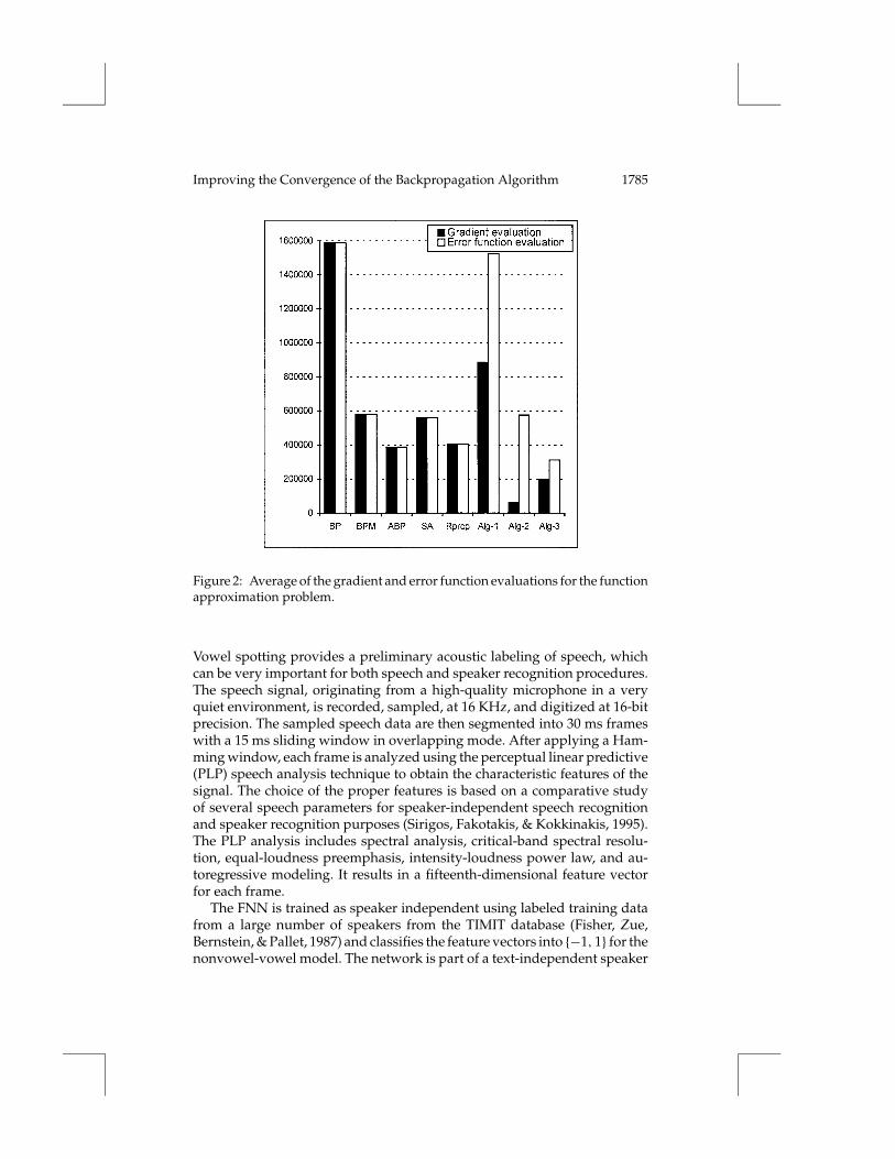
1994). Training is considered successful when E ≤ 0.0125. Comparative re-sults are shown in Figure 2 and in Table 3, where the abbreviations are as inTable 2.

In the third experiment a 15-15-1 FNN (240 weights and 16 biases), basedon neurons of hyperbolic tangent activations, is used for vowel spotting.

1784G

.D.M

agoulas,M.N

.Vrahatis,and

G.S.A

ndroulakis

Table 3: Comparative Results for the Function Approximation Problem.



BP 1,588,720 1,069,320 284,346/4,059,620 1,588,720 1,069,320 284,346/4,059,620 100BPM 578,848 189,574 243,111/882,877 578,848 189,574 243,111/882,877 100ABP 388,457 160,735 99,328/694,432 388,457 160,735 99,328/694,432 100SA 559,684 455,807 94,909/1,586,652 559,684 455,807 94,909/1,586,652 85Rprop 405,033 93,457 60,162/859,904 405,033 93,457 60,162/859,904 80Algorithm-1 886,364 409,237 287,562/1,734,820 1,522,890 852,776 495,348/352,5231 100Algorithm-2 62,759 15,851 25,282/81,488 576,532 1 48,064 244,698/768,254 100Algorithm-3 198,172 82,587 101,460/369,652 311,773 116,958 148,256/539,137 100


Figure 2: Average of the gradient and error function evaluations for the functionapproximation problem.

Vowel spotting provides a preliminary acoustic labeling of speech, whichcan be very important for both speech and speaker recognition procedures.The speech signal, originating from a high-quality microphone in a veryquiet environment, is recorded, sampled, at 16 KHz, and digitized at 16-bitprecision. The sampled speech data are then segmented into 30 ms frameswith a 15 ms sliding window in overlapping mode. After applying a Ham-ming window, each frame is analyzed using the perceptual linear predictive(PLP) speech analysis technique to obtain the characteristic features of thesignal. The choice of the proper features is based on a comparative studyof several speech parameters for speaker-independent speech recognitionand speaker recognition purposes (Sirigos, Fakotakis, & Kokkinakis, 1995).The PLP analysis includes spectral analysis, critical-band spectral resolu-tion, equal-loudness preemphasis, intensity-loudness power law, and au-toregressive modeling. It results in a fifteenth-dimensional feature vectorfor each frame.

The FNN is trained as speaker independent using labeled training datafrom a large number of speakers from the TIMIT database (Fisher, Zue,Bernstein, & Pallet, 1987) and classifies the feature vectors into {−1, 1} for thenonvowel-vowel model. The network is part of a text-independent speaker


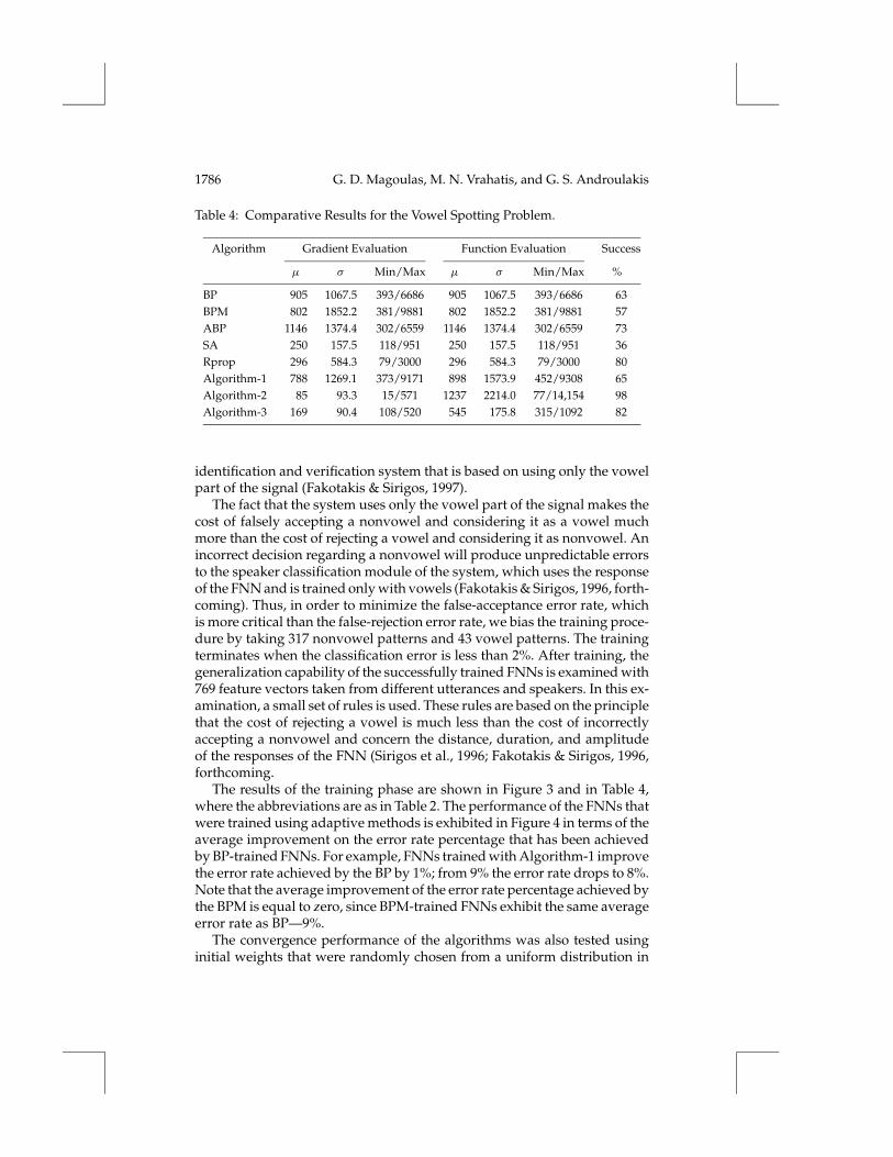
Table 4: Comparative Results for the Vowel Spotting Problem.



BP 905 1067.5 393/6686 905 1067.5 393/6686 63BPM 802 1852.2 381/9881 802 1852.2 381/9881 57ABP 1146 1374.4 302/6559 1146 1374.4 302/6559 73SA 250 157.5 118/951 250 157.5 118/951 36Rprop 296 584.3 79/3000 296 584.3 79/3000 80Algorithm-1 788 1269.1 373/9171 898 1573.9 452/9308 65Algorithm-2 85 93.3 15/571 1237 2214.0 77/14,154 98Algorithm-3 169 90.4 108/520 545 175.8 315/1092 82

identification and verification system that is based on using only the vowelpart of the signal (Fakotakis & Sirigos, 1997).

The fact that the system uses only the vowel part of the signal makes thecost of falsely accepting a nonvowel and considering it as a vowel muchmore than the cost of rejecting a vowel and considering it as nonvowel. Anincorrect decision regarding a nonvowel will produce unpredictable errorsto the speaker classification module of the system, which uses the responseof the FNN and is trained only with vowels (Fakotakis & Sirigos, 1996, forth-coming). Thus, in order to minimize the false-acceptance error rate, whichis more critical than the false-rejection error rate, we bias the training proce-dure by taking 317 nonvowel patterns and 43 vowel patterns. The trainingterminates when the classification error is less than 2%. After training, thegeneralization capability of the successfully trained FNNs is examined with769 feature vectors taken from different utterances and speakers. In this ex-amination, a small set of rules is used. These rules are based on the principlethat the cost of rejecting a vowel is much less than the cost of incorrectlyaccepting a nonvowel and concern the distance, duration, and amplitudeof the responses of the FNN (Sirigos et al., 1996; Fakotakis & Sirigos, 1996,forthcoming.

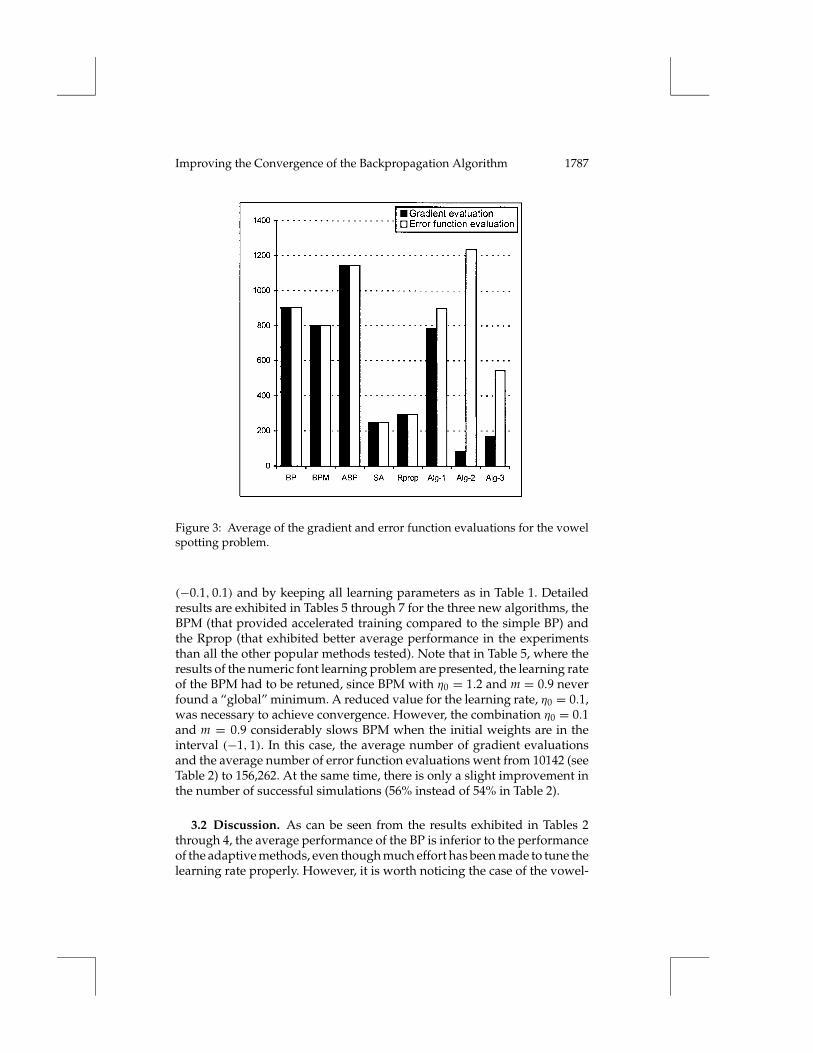
The results of the training phase are shown in Figure 3 and in Table 4,where the abbreviations are as in Table 2. The performance of the FNNs thatwere trained using adaptive methods is exhibited in Figure 4 in terms of theaverage improvement on the error rate percentage that has been achievedby BP-trained FNNs. For example, FNNs trained with Algorithm-1 improvethe error rate achieved by the BP by 1%; from 9% the error rate drops to 8%.Note that the average improvement of the error rate percentage achieved bythe BPM is equal to zero, since BPM-trained FNNs exhibit the same averageerror rate as BP—9%.

The convergence performance of the algorithms was also tested usinginitial weights that were randomly chosen from a uniform distribution in


Figure 3: Average of the gradient and error function evaluations for the vowelspotting problem.

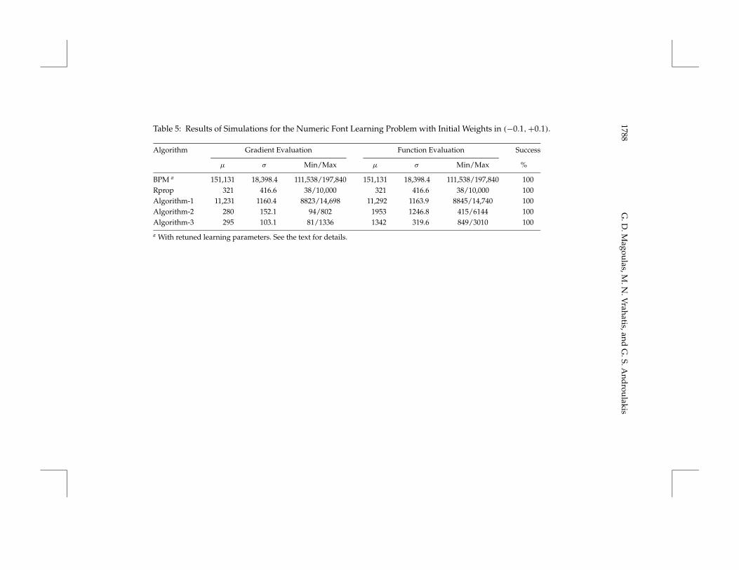
(−0.1, 0.1) and by keeping all learning parameters as in Table 1. Detailedresults are exhibited in Tables 5 through 7 for the three new algorithms, theBPM (that provided accelerated training compared to the simple BP) andthe Rprop (that exhibited better average performance in the experimentsthan all the other popular methods tested). Note that in Table 5, where theresults of the numeric font learning problem are presented, the learning rateof the BPM had to be retuned, since BPM with η0 = 1.2 and m = 0.9 neverfound a “global” minimum. A reduced value for the learning rate, η0 = 0.1,was necessary to achieve convergence. However, the combination η0 = 0.1and m = 0.9 considerably slows BPM when the initial weights are in theinterval (−1, 1). In this case, the average number of gradient evaluationsand the average number of error function evaluations went from 10142 (seeTable 2) to 156,262. At the same time, there is only a slight improvement inthe number of successful simulations (56% instead of 54% in Table 2).

3.2 Discussion. As can be seen from the results exhibited in Tables 2through 4, the average performance of the BP is inferior to the performanceof the adaptive methods, even though much effort has been made to tune thelearning rate properly. However, it is worth noticing the case of the vowel-

1788G

.D.M

agoulas,M.N

.Vrahatis,and

G.S.A

ndroulakis

Table 5: Results of Simulations for the Numeric Font Learning Problem with Initial Weights in (−0.1,+0.1).



BPM a 151,131 18,398.4 111,538/197,840 151,131 18,398.4 111,538/197,840 100Rprop 321 416.6 38/10,000 321 416.6 38/10,000 100Algorithm-1 11,231 1160.4 8823/14,698 11,292 1163.9 8845/14,740 100Algorithm-2 280 152.1 94/802 1953 1246.8 415/6144 100Algorithm-3 295 103.1 81/1336 1342 319.6 849/3010 100

a With retuned learning parameters. See the text for details.

Improving

theC

onvergenceofthe

Backpropagation

Algorithm

1789

Table 6: Results of Simulations for the Function Approximation Problem with Initial Weights in (−0.1,+0.1).



BPM 486,120 76,102 139,274/1028,933 486,120 76,102 139,274/1,028,933 100Rprop 350,732 83,734 64,219/553,219 350,732 83,734 64,219/553,219 48Algorithm-1 1,033,520 419,016 484,846/1,633,410 2,341,300 1,102,970 917,181/4,235,960 100Algorithm-2 65,028 21,625 30,067/129,025 495,796 238,001 227,451/979,000 100Algorithm-3 146,166 54,119 73,293/245,255 222,947 88,980 107,292/389,373 100


Figure 4: Average improvement of the error rate percentage achieved by theadaptive methods over BP for the vowel spotting problem.

Table 7: Results of Simulations for the Vowel Spotting Problem with InitialWeights in (−0.1,+0.1).



BPM 1493 837.2 532/15,873 1493 837.2 532/15,873 62Rprop 513 612.8 53/11,720 513 612.8 53/11,720 82Algorithm-1 1684 1267.2 864/9286 2148 1290.3 1214/9644 74Algorithm-2 88 137.8 44/680 1909 2105.9 327/14,742 98Algorithm-3 206 127.7 117/508 566 176.5 321/1420 92

spotting problem, where the BP algorithm is sufficiently fast, needing, onaverage, fewer gradient and function evaluations than the ABP algorithm.It also exhibits less error function evaluations but needs significantly more(820) gradient evaluations than Algorithm-2.

The use of a fixed momentum term helps accelerate the BP training butdeteriorates the reliability of the algorithm in two out of the three experi-ments, when initial weights are in the interval (−1, 1). BPM with smaller ini-tial weights, in the interval (−0.1, 0.1), provides more reliable training (see


Tables 5 through 7). However, the use of small weights results in reducedtraining time only in the function approximation problem (see Table 6).

In the vowel spotting problem, BPM outperforms ABP with respect tothe number of gradient and error function evaluations. It also outperformsAlgorithm-1 and Algorithm-2 regarding the average number of error func-tion evaluations. Unfortunately, BPM has a smaller percentage of successand requires more gradient evaluations than Algorithm-1 and Algorithm-2.Regarding the generalization capability of the algorithm, it is almost similarto the BP generalization in both weight ranges and is inferior to all the otheradaptive methods.

Algorithm-1 has the ability to handle arbitrary large learning rates. Ac-cording to the experiments we performed, the exponential schedule ofAlgorithm-1 appears fast enough for certain neural network applications,resulting in faster training when compared with the BP, but in slower train-ing when compared with BPM and the other adaptive BP methods. Specif-ically, Algorithm-1 requires significantly more gradient and error functionevaluations in the function approximation problem than all the other adap-tive methods when the initial weights are in the range (−0.1, 0.1). In thevowel spotting problem, its convergence speed is also reduced comparedto its own speed in the interval (−1, 1). However, it reveals a higher per-centage of successful runs.

In conclusion, regarding training speed, Algorithm-1 can only be con-sidered as an alternative to the BP algorithm since it allows training witharbitrary large initial learning rates and reduces the necessary number ofgradient evaluations. In this respect, steps 2 and 3 of Algorithm-1 can serveas a heuristic free tuning mechanism that can be incorporated into an adap-tive training algorithm to guarantee that a weight update provides sufficientreduction in the error function at each iteration. In this way, the user canavoid spikes in the error function as result of the “jumpy” behavior of theweights. It is well known that this kind of behavior pushes the neurons intosaturation, causing the training algorithm to be trapped in an undesiredlocal minimum (Kung, Diamantaras, Mao, & Taur, 1991; Parlos, Fernandez,Atiya, Muthusami, & Tsai, 1994). Regarding convergence reliability andgeneralization, Algorithm-1 outperforms BP and BPM.

On average, Algorithm-2 needs fewer gradient evaluations than all theother methods tested. This fact is considered quite important, especially inlearning tasks that the algorithm exhibits a high percentage of success. In ad-dition Algorithm-2 does not heavily depend on the range of initial weights,provides better generalization than BP, BPM, and ABP, and does not useany initial learning rate. This algorithm exhibits the best performance withrespect to the percentage of successful runs in all problems tested, includingthe vowel spotting problem, where it had the highest percentage of success.The algorithm takes advantage of its inherent mechanism to prevent entrap-ment in the neighborhood of a local minimum. With respect to the meannumber of gradient evaluations, Algorithm-2 exhibits the best average in


the second and third experiments. In addition, it clearly outperforms BPand BPM in the first two experiments with respect to the mean number oferror function evaluations. However, since fewer runs have converged toa global minimum for the BP in the third experiment, BP reveals a lowermean number of function evaluations for the converged runs.

Algorithm-3 exploits knowledge related to the local shape of the errorsurface in the form of the Lipschitz constant estimation. The algorithm ex-hibits a good average behavior with regard to the percentage of success andthe mean number of error function evaluations. Regarding the mean num-ber of gradient evaluations, which are considered more costly than errorfunction evaluations, it outperforms all other methods tested in the secondand third experiments (except Algorithm-2). In the case of the first experi-ment, Algorithm-3 needs more gradient and error function evaluations thanRprop, but provides more stable learning and thus a greater possibility ofsuccessful training, when the initial weights are in the range (−1, 1). In addi-tion, the algorithm appears, on average, less sensitive to the range of initialweights than the other methods that adapt a different learning rate for eachweight, SA and Rprop.

It is also interesting to observe the performance of the rest of the adaptivemethods. The method of Vogl et al. (1988), ABP, has a good average perfor-mance on all problems, while the method of Silva and Almeida (1990), SA,although it provides rapid convergence, has the lowest percentage of successof all adaptive algorithms tested in the two pattern recognition problems(numeric font and vowel spotting). This algorithm exhibits stability prob-lems because the learning rates increase exponentially when many iterationsare performed successively. This behavior results in minimization steps thatincrease some weights by large amounts, pushing the outputs of some neu-rons into saturation and consequently into convergence to a local minimumor maximum. The Rprop algorithm is definitely faster than the other al-gorithms in the numeric font problem, but it has a lower percentage ofsuccess than the new methods. In the vowel spotting experiment, it exhibitsa lower mean number of error function evaluations than the proposed meth-ods. However, it requires more gradient evaluations than Algorithm-2 andAlgorithm-3, which are considered more costly. When initial weights in therange (−0.1, 0.1) are used, the behavior of the Rprop highly depends on thelearning task. To be more specific, in the numeric font learning experimentand in vowel spotting, its percentages of successful runs are 100% and 82%,respectively, with a small additional cost in the average error function andgradient evaluations. On the other hand, in the function approximation ex-periment, Rprop’s convergence speed is improved, but its percentage of suc-cess is significantly reduced. This seems to be caused by shallow local min-ima that prevent the algorithm from reaching the desired global minimum.

Finally, the results in the vowel spotting experiment, with respect tothe generalization performance of the tested algorithms, indicate that theincreased convergence rates achieved by the adaptive algorithms by no


means affect their generalization capability. On the contrary, the generaliza-tion performance of these methods is better than the BP method. In fact, theclassification accuracy achieved by Algorithm-3 and Rprop is the best of allthe tested methods.

4 Conclusions

In this article, we reported on three new gradient-based training methods.These new methods ensure global convergence, that is, convergence to alocal minimizer of the error function from any starting point. The proposedalgorithms have been compared with several training algorithms, and theirefficiency has been numerically confirmed by the experiments we presented.The new algorithms exhibit the following features:

• They combine inexact line search techniques with second-order relatedinformation without calculating second derivatives.

• They provide accelerated training without oscillation by ensuring thatthe error function is sufficiently decreased with every iteration.

• Algorithm-1 and Algorithm-3 allow convergence for wide variationsin the learning-rate values, while Algorithm-2 eliminates the need foruser-defined learning parameters.

• Their convergence is guaranteed under suitable assumptions. Specifi-cally, the convergence characteristics of Algorithm-2 and Algorithm-3are not sensitive to the two initial weight ranges tested.

• They provide stable learning and therefore a greater possibility of goodperformance.

Acknowledgments

We acknowledge the contributions of N. Fakotakis and J. Sirigos in thevowel spotting experiments. We also thank the reviewers for helpful com-ments and careful readings. This work was partially supported by the GreekGeneral Secretariat for Research and Technology of the Greek Ministry ofIndustry under a 5ENE1 grant.

References

Altman, M. (1961). Connection between gradient methods and Newton’smethod for functionals. Bull. Acad. Polon. Sci. Ser. Sci. Math. Astronom. Phys.,9, 877–880.

Armijo, L. (1966). Minimization of functions having Lipschitz continuous firstpartial derivatives. Pacific Journal of Mathematics, 16, 1–3.

Battiti, R. (1989). Accelerated backpropagation learning: Two optimizationmethods. Complex Systems, 3, 331–342.


Battiti, R. (1992). First- and second-order methods for learning: Between steepestdescent and Newton’s method. Neural Computation, 4, 141–166.

Becker, S., & Le Cun, Y. (1988). Improving the convergence of the back–propagation learning with second order methods. In D. S. Touretzky, G. E.Hinton, & T. J. Sejnowski (Eds.), Proceedings of the 1988 Connectionist ModelsSummer School (pp. 29–37). San Mateo, CA: Morgan Kaufmann.

Booth, A. (1949). An application of the method of steepest descent to the solutionof systems of nonlinear simultaneous equations. Quart. J. Mech. Appl. Math.,2, 460–468.

Cauchy, A. (1847). Methode generale pour la resolution des systemesd’equations simultanees. Comp. Rend. Acad. Sci. Paris, 25, 536–538.

Chan, L. W., & Fallside, F. (1987). An adaptive training algorithm for back–propagation networks. Computers, Speech and Language, 2, 205–218.

Darken, C., Chiang, J., & Moody, J. (1992). Learning rate schedules for fasterstochastic gradient search. In Proceedings of the IEEE 2nd Workshop on NeuralNetworks for Signal Processing (pp. 3–12).

Demuth, H., & Beale, M. (1992). Neural network toolbox user’s guide. Natick, MA:MathWorks.

Dennis, J. E., & More, J. J. (1977). Quasi-Newton methods, motivation and theory.SIAM Review, 19, 46–89.

Dennis, J. E., & Schnabel, R. B. (1983). Numerical methods for unconstrained opti-mization and nonlinear equations. Englewood Cliffs, NJ: Prentice-Hall.

Fahlman, S. E. (1989). Faster-learning variations on back–propagation: An em-pirical study. In D. S. Touretzky, G. E. Hinton, & T. J. Sejnowski (Eds.), Proceed-ings of the 1988 Connectionist Models Summer School (pp. 38–51). San Mateo,CA: Morgan Kaufmann.

Fakotakis, N., & Sirigos, J. (1996). A high-performance text-independent speakerrecognition system based on vowel spotting and neural nets. In Proceedingsof the IEEE International Conference on Acoustic Speech and Signal Processing, 2,661–664.

Fakotakis, N., & Sirigos, J. (forthcoming). A high-performance text-independentspeaker identification and verification system based on vowel spotting andneural nets. IEEE Trans. Speech and Audio processing.

Fisher, W., Zue, V., Bernstein, J., & Pallet, D. (1987). An acoustic-phonetic database. Journal of Acoustical Society of America, Suppl. A, 81, 581–592.

Goldstein, A. A. (1962). Cauchy’s method of minimization. Numerische Mathe-matik, 4, 146–150.

Gori, M., & Tesi, A. (1992). On the problem of local minima in backpropagation.IEEE Trans. Pattern Analysis and Machine Intelligence, 14, 76–85.

Hirose, Y., Yamashita, K., & Hijiya, S. (1991). Back–propagation algorithm whichvaries the number of hidden units. Neural Networks, 4, 61–66.

Hoehfeld, M., & Fahlman, S. E. (1992). Learning with limited numerical precisionusing the cascade-correlation algorithm. IEEE Trans. on Neural Networks, 3,602–611.

Hsin, H.-C., Li, C.-C., Sun, M., & Sclabassi, R. J. (1995). An adaptive training al-gorithm for back–propagation neural networks. IEEE Transactions on System,Man and Cybernetics, 25, 512–514.


Jacobs, R. A. (1988). Increased rates of convergence through learning rate adap-tation. Neural Networks, 1, 295–307.

Kelley, C. T. (1995). Iterative methods for linear and nonlinear equations. Philadel-phia: SIAM.

Kung, S. Y., Diamantaras, K., Mao, W. D., Taur, J. S. (1991). Generalized percep-tron networks with nonlinear discriminant functions. In R. J. Mammone &Y. Y. Zeevi (Eds.), Neural networks theory and applications (pp. 245–279). NewYork: Academic Press.

Le Cun, Y., Simard, P. Y., & Pearlmutter, B. A. (1993). Automatic learning ratemaximization by on–line estimation of the Hessian’s eigenvectors. In S. J.Hanson, J. D. Cowan, & C. L. Giles (Eds.), Advances in neural informationprocessing systems, 5 (pp. 156–163). San Mateo, CA: Morgan Kaufmann.

Lee, Y., Oh, S.-H., & Kim, M. W. (1993). An analysis of premature saturation inbackpropagation learning. Neural Networks, 6, 719–728.

Lisboa, P. J. G., & Perantonis S. J. (1991). Complete solution of the local minimain the XOR problem. Network, 2, 119–124.

Magoulas, G. D., Vrahatis, M. N., & Androulakis, G. S. (1996). A new methodin neural network supervised training with imprecision. In Proceedings of theIEEE 3rd International Conference on Electronics, Circuits and Systems (pp. 287–290).

Magoulas, G. D., Vrahatis, M. N., & Androulakis, G. S. (1997). Effective back–propagation with variable stepsize. Neural Networks, 10, 69–82.

Magoulas, G. D., Vrahatis, M. N., Grapsa, T. N., & Androulakis, G. S. (1997). Neu-ral network supervised training based on a dimension reducing method.In S. W. Ellacot, J. C. Mason, & I. J. Anderson (Eds.), Mathematics of neu-ral networks: Models, algorithms and applications (pp. 245–249). Norwell, MA:Kluwer.

Møller, M. F. (1993). A scaled conjugate gradient algorithm, for fast supervisedlearning. Neural Networks, 6, 525–533.

Nocedal, J. (1991). Theory of algorithms for unconstrained optimization. ActaNumerica, 199–242.

Ortega, J. M., & Rheinboldt, W. C. (1970). Iterative solution of nonlinear equationsin several variables. New York: Academic Press.

Parker, D. B. (1987). Optimal algorithms for adaptive networks: Second orderback–propagation, second order direct propagation, and second order Heb-bian learning. In Proceedings of the IEEE International Conference on NeuralNetworks, 2, 593–600.

Parlos, A. G., Fernandez, B., Atiya, A. F., Muthusami, J., & Tsai, W. K. (1994).An accelerated learning algorithm for multilayer perceptron networks. IEEETrans. on Neural Networks, 5, 493–497.

Pearlmutter, B. (1992). Gradient descent: Second–order momentum and saturat-ing error. In J. E. Moody, S. J. Hanson, & R. P. Lippmann (Eds)., Advances inneural information processing systems, 4 (pp. 887–894). San Mateo, CA: MorganKaufmann.

Pfister, M., & Rojas, R. (1993). Speeding-up backpropagation—A comparisonof orthogonal techniques. In Proceedings of the Joint Conference on Neural Net-works. (pp. 517–523). Nagoya, Japan.


Riedmiller, M. (1994). Advanced supervised learning in multi-layer percept-rons—From backpropagation to adaptive learning algorithms. InternationalJournal of Computer Standards and Interfaces, special issue, 5.

Riedmiller, M., & Braun, H. (1993). A direct adaptive method for faster backprop-agation learning: The Rprop algorithm. In Proceedings of the IEEE InternationalConference on Neural Networks. (pp. 586–591). San Francisco, CA.

Rigler, A. K., Irvine, J. M., & Vogl, T. P. (1991). Rescaling of variables in back-propagation learning. Neural Networks, 4, 225–229.

Rojas, R. (1996). Neural networks: A systematic introduction. Berlin: Springer-Verlag.

Rumelhart, D. E., Hinton, G. E., & Williams, R. J. (1986). Learning internal rep-resentations by error propagation. In D. E. Rumelhart, & J. L. McClelland(Eds.), Parallel distributed processing: Explorations in the microstructure of cogni-tion (Vol. 1, pp. 318–362). Cambridge, MA: MIT Press.

Schaffer, J., Whitley, D., & Eshelman, L. (1992). Combinations of genetic algo-rithms and neural networks: A survey of the state of the art. In Proceedingsof the International Workshop on Combinations of Genetic Algorithms and NeuralNetworks (pp. 1–37). Los Alamitos, CA: IEEE Computer Society Press.

Shultz, G. A., Schnabel, R. B., & Byrd, R. H. (1982). A family of trust region based al-gorithms for unconstrained minimization with strong global convergence properties(Tech. Rep. No. CU-CS216-82). University of Colorado.

Silva, F., & Almeida, L. (1990). Acceleration techniques for the back–propagationalgorithm. Lecture Notes in Computer Science, 412, 110–119.

Sirigos, J., Darsinos, V., Fakotakis, N., & Kokkinakis, G. (1996). Vowel/non-vowel decision using neural networks and rules. In Proceedings of the 3rd IEEEInternational Conference on Electronics, Circuits, and Systems (pp. 510–513).

Sirigos, J., Fakotakis, N., & Kokkinakis, G. (1995). A comparison of several speechparameters for speaker independent speech recognition and speaker recog-nition. In Proceedings of the 4th European Conference of Speech Communicationsand Technology.

Van der Smagt, P. P. (1994). Minimization methods for training feedforwardneural networks. Neural Networks, 7, 1–11.

Vogl, T. P, Mangis, J. K., Rigler, J. K., Zink, W. T., & Alkon, D. L. (1988). Acceler-ating the convergence of the backpropagation method. Biological Cybernetics,59, 257–263.

Watrous, R. L. (1987). Learning algorithms for connectionist networks: Appliedgradient of nonlinear optimization. In Proceedings of the IEEE InternationalConference on Neural Networks, 2, 619–627.

Wessel, L. F., & Barnard, E. (1992). Avoiding false local minima by proper ini-tialization of connections. IEEE Trans. Neural Networks, 3, 899–905.

Wolfe, P. (1969). Convergence conditions for ascent methods. SIAM Review, 11,226–235.

Wolfe, P. (1971). Convergence conditions for ascent methods. II: Some correc-tions. SIAM Review, 13, 185–188.

Received April 8, 1997; accepted September 21, 1998.

Documents

Improving the convergence of the back-propagation algorithm using