Error Back Propagation Algorithm

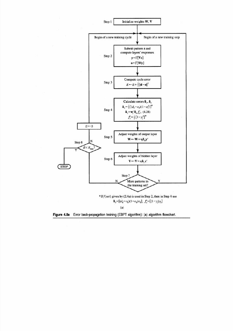
8/7/2019 Error Back Propagation Algorithm

http://slidepdf.com/reader/full/error-back-propagation-algorithm 1/14

ERROR BACKPROPAGATION ALGORITHM

Why Error Back Propagation Algorithm is required?

Lack of suitable training methods for multilayer perceptrons (MLP)s led to a waning of

interest in NN in 1960s and 1970s. This was changed by the reformulation of the

backPropagation training method for MLPs in the mid-1980s by Rumelhart et al.

Backpropagation was created by generalizing the Widrow-Hoff learning rule to multiple-layer networks and nonlinear differentiable transfer functions. Standard

backpropagation is a gradient descent algorithm, as is the Widrow-Hoff learning rule, in

which the network weights are moved along the negative of the gradient of the

performance function. The term backpropagation refers to the manner in which the

gradient is computed for nonlinear multilayer networks.

As in simple cases of the delta learning rule training studied before, input patterns are

submitted during the back-propagation training sequentially. If a pattern is submitted

and its classification or association is determined to be erroneous, the synaptic weights

as well as the thresholds are adjusted so that the current least mean square classification

error is reduced. The input l output mapping, comparison of target and actual values,and adjustment, if needed, continue until all mapping examples from the training set are

learned within an acceptable overall error. Usually, mapping error is cumulative and

computed over the full training set.

During the association or classification phase, the trained neural network itself operates

in a feedforward manner. However, the weight adjustments enforced by the learning

rules propagate exactly backward from the output layer through the so-called "hidden

layers" toward the input layer.



The input and output values of the network are denoted y j and ok , respectively. We thus,

denote yj, for j = 1, 2, . . . , J, and ok, for k = 1, 2, . . . , K, as signal values at the j'th

column of nodes, and k'th column of nodes, respectively. As before, the weight wkj

connects the output of the j'th neuron with the input to the k'th neuron.

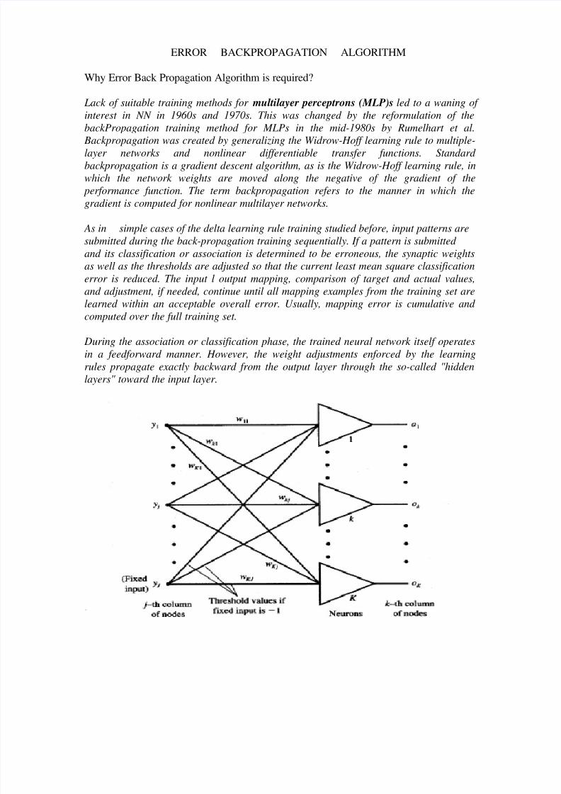
The activation function netk

of layer k is expressed as

The error expression generalized to include all squared errors at the outputs k=1,2,3…K

Where p is a specific pattern and p=1 2……P

Delta learning rule can be formally derived for a multiperceptron layer. Assumptions

made are

1. gradient descent search is performed to reduce the error Ep through adjustments

of weights

2. threshold values are adjustable with other weights and no distinction is made

between threshold and weights during learning

3. Fixed input of value during both the training and recall phases

Minimization of error requires the weight changes to be in the negative gradient

direction. Individual weight adjustments are computed as follows

Error E is defined in Eqn:2.

Now for each node in layer k where k=1,2,….K

Eqn. 1

Eqn:2

Eqn:3



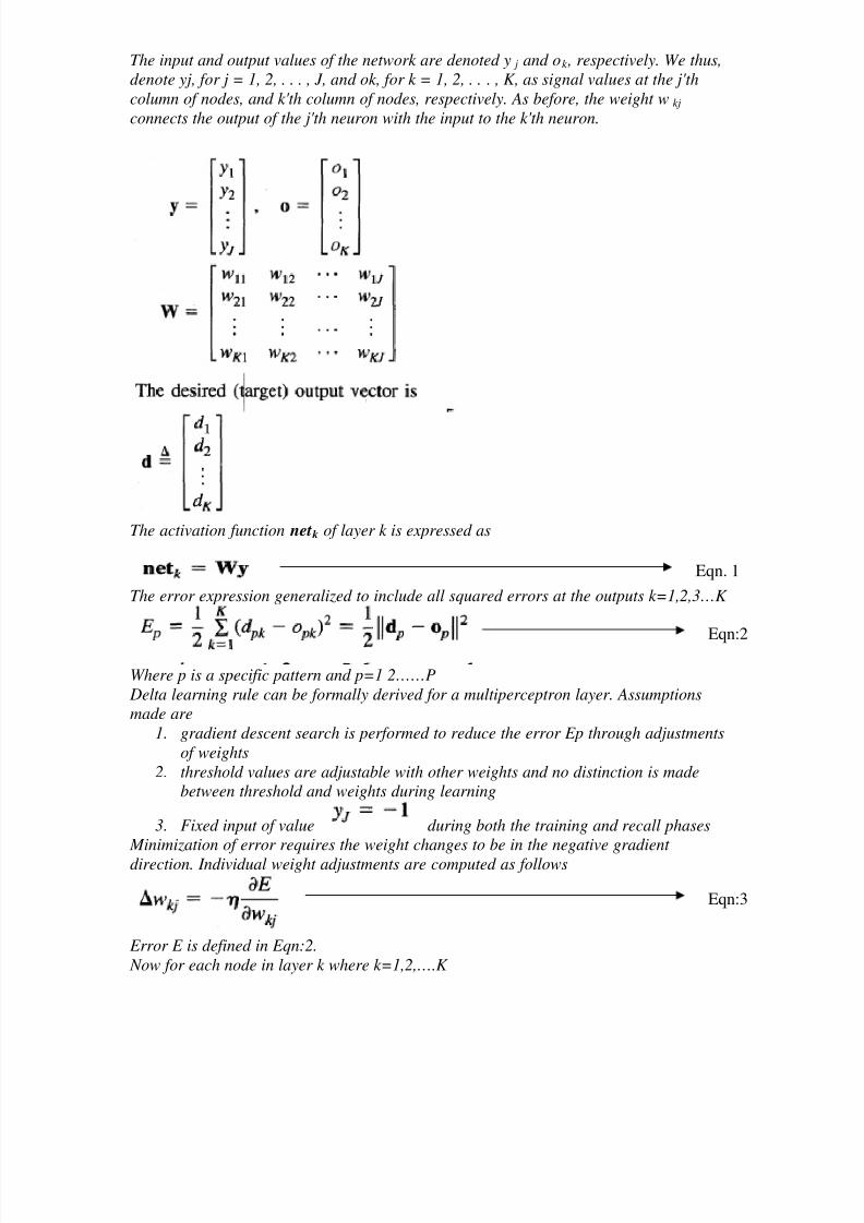
And the corresponding neuron output is given by

Since

Substituting Eqn 8, Eqn 6 in Eqn 7 we get

The weight adjustment formula of Eqn 3 can accordingly be rewritten as

Eqn 10 represents the general formula for delta training/learning weight adjustments for a single-layer network. It also follows that the adjustments of weight wkj is proportional

to the input activation yj, and to the error signal value at the kth neuron’s output.

The delta value needs to be explicitly computed for specifically chosen activation

functions.

Eqn:4

Eqn:5

Eqn:6

Eqn:7

Eqn:8

Eqn:9

Eqn: 10



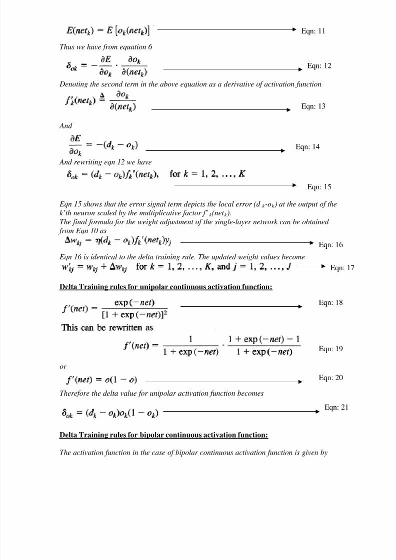
Thus we have from equation 6

Denoting the second term in the above equation as a derivative of activation function

And

And rewriting eqn 12 we have

Eqn 15 shows that the error signal term depicts the local error (d k -ok ) at the output of the

k’th neuron scaled by the multiplicative factor f’k (net k

The final formula for the weight adjustment of the single-layer network can be obtained

from Eqn 10 as

).

Eqn 16 is identical to the delta training rule. The updated weight values become

Delta Training rules for unipolar continuous activation function:

or

Therefore the delta value for unipolar activation function becomes

Delta Training rules for bipolar continuous activation function:

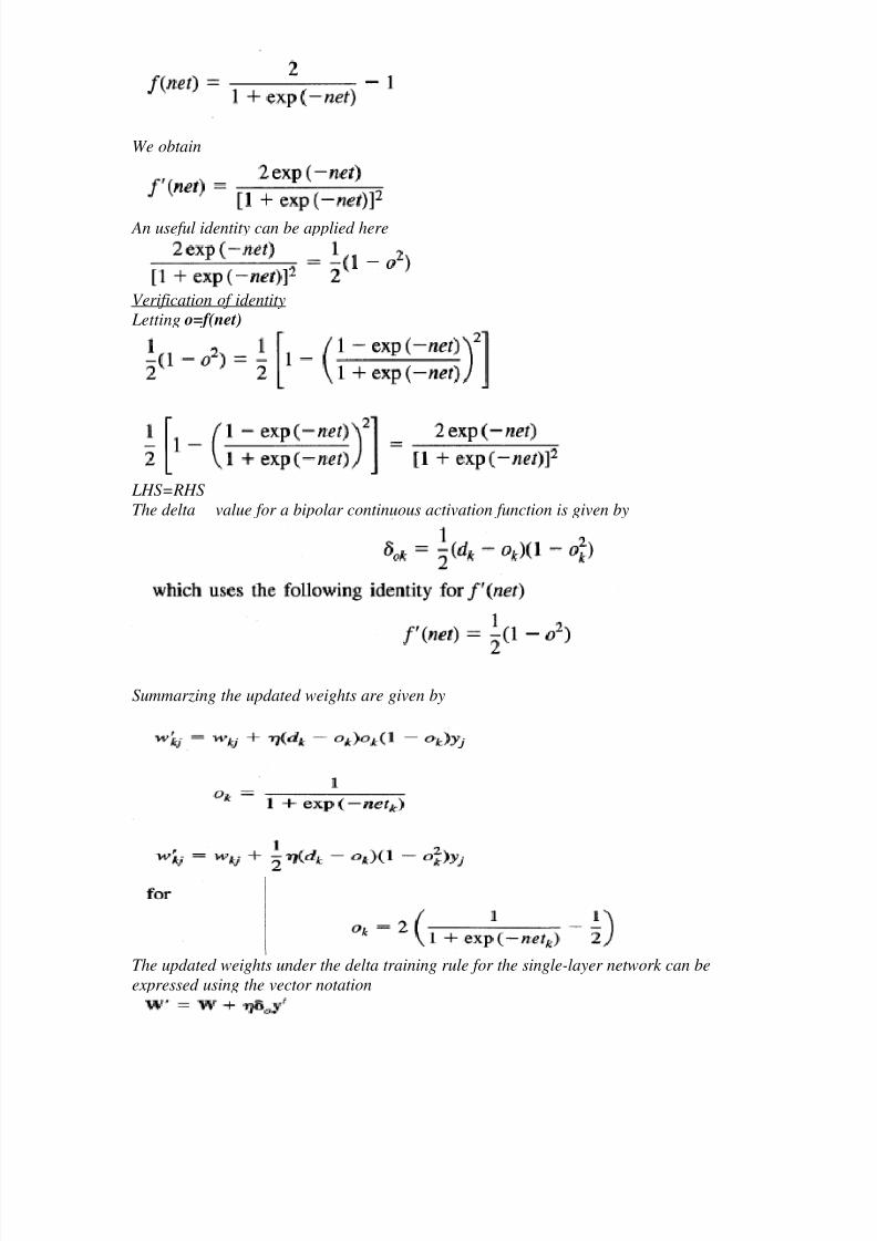
The activation function in the case of bipolar continuous activation function is given by

Eqn: 11

Eqn: 12

Eqn: 13

Eqn: 14

Eqn: 15

Eqn: 16

Eqn: 17

Eqn: 18

Eqn: 19

Eqn: 20

Eqn: 21



We obtain

An useful identity can be applied here

Letting o=f(net)

Verification of identity

LHS=RHS

The delta value for a bipolar continuous activation function is given by

Summarzing the updated weights are given by

The updated weights under the delta training rule for the single-layer network can be

expressed using the vector notation



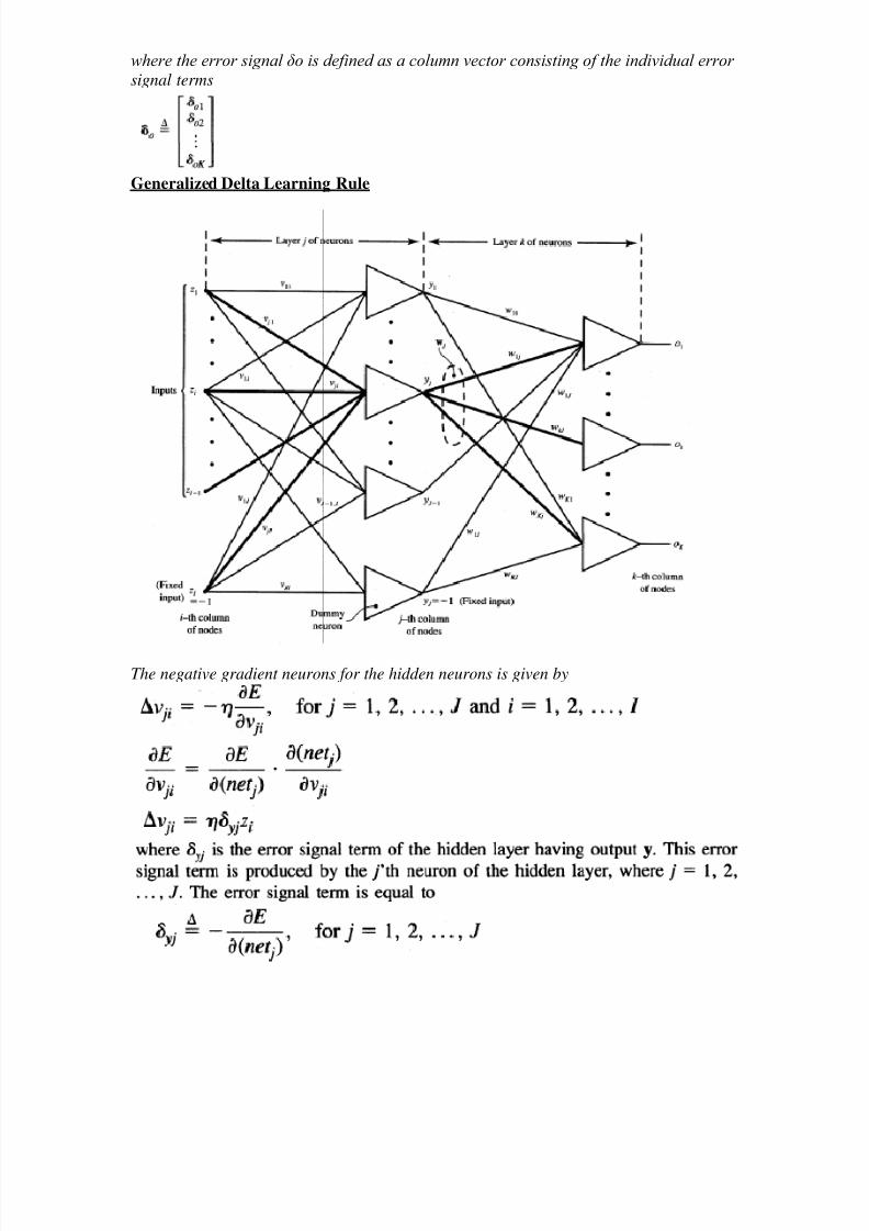
where the error signal δo is defined as a column vector consisting of the individual error signal terms

Generalized Delta Learning Rule

The negative gradient neurons for the hidden neurons is given by









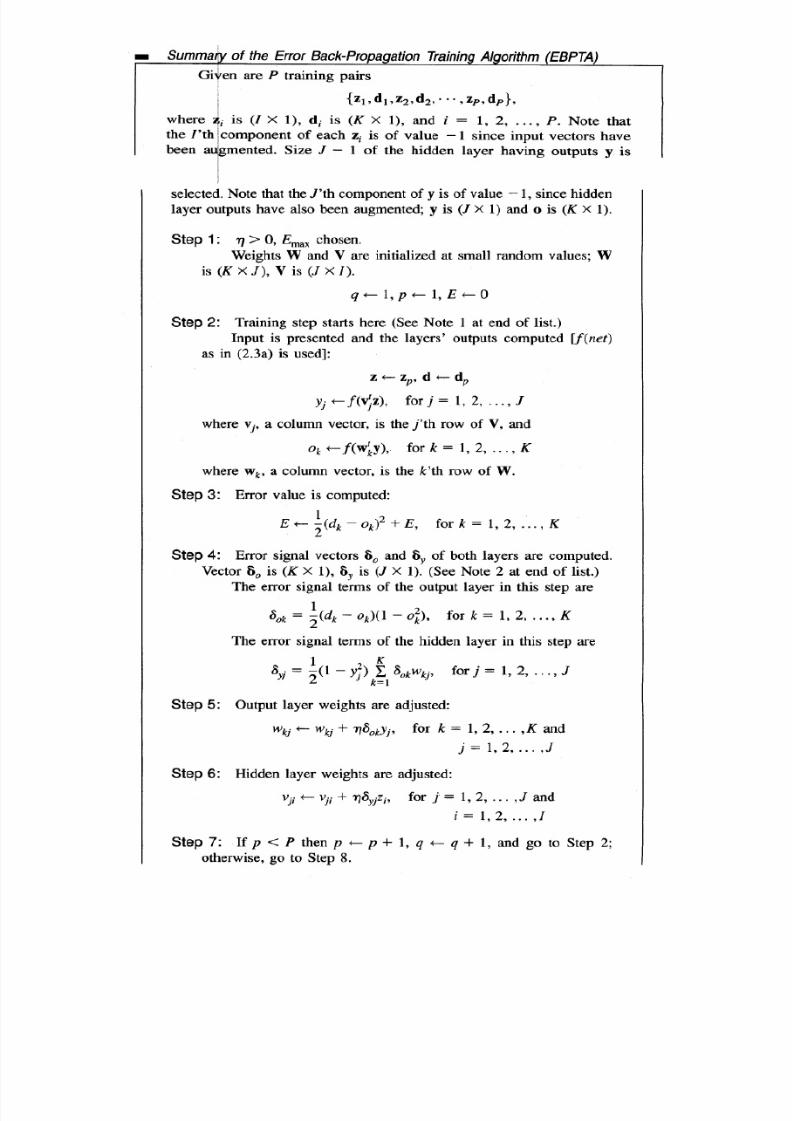
There are two modes of updation of weights1. Batch mode

2. Incremental mode

When the weights are being changed immediately after a training pattern is presented

then it is called as incremental approach.

When the weights are changed only after all the training patterns are presented then it is

called as batch mode. This mode requires additional local storage for each connection to

maintain the immediate weight changes.

The BP learning algorithm is an example of optimization problem. [Note:- an

optimization problem is the problem of finding the best solution from all feasiblesolutions]. The essence of the error back-propagation algorithm is the evaluation of the

contribution of each particular weight to the output error. There are many difficulties

that arise in the implementation of the algorithm. One of the problems is that the error

minimization procedure may produce only a local minimum of the error function.



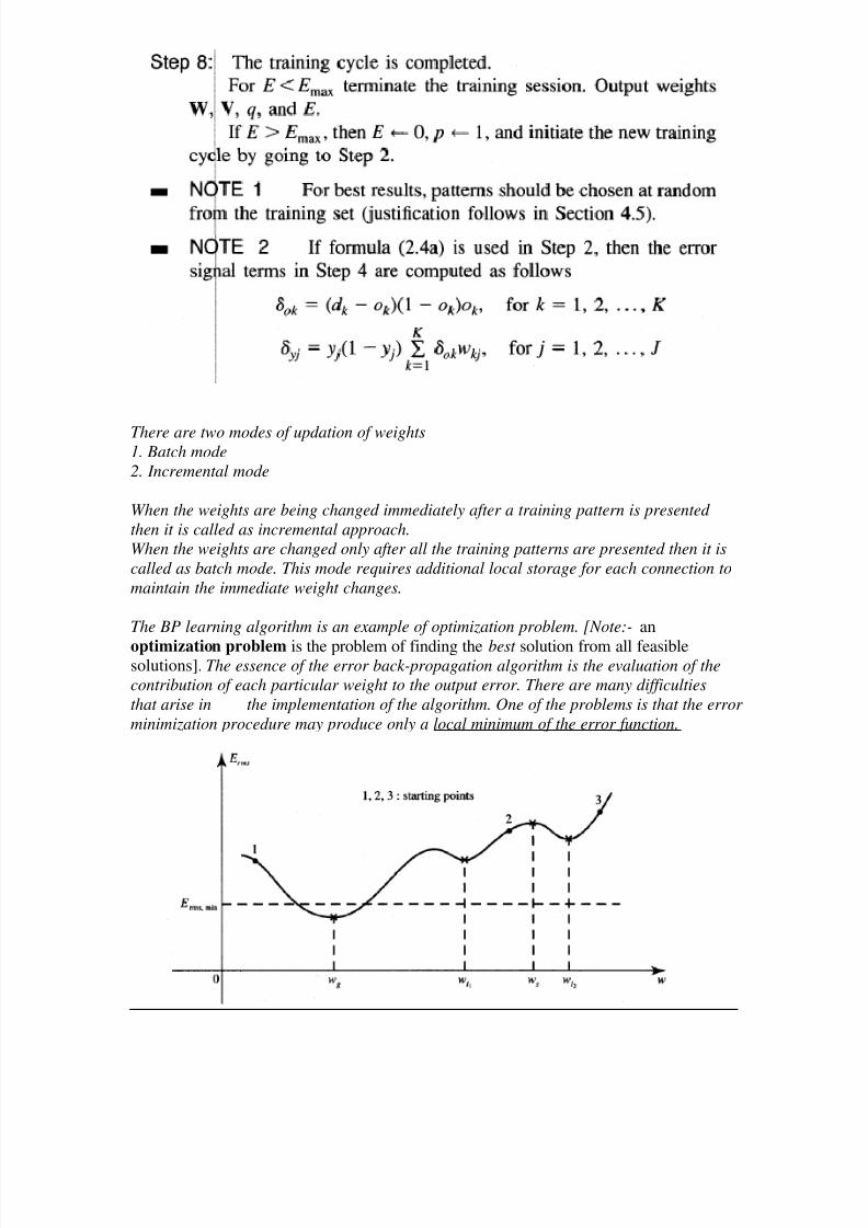
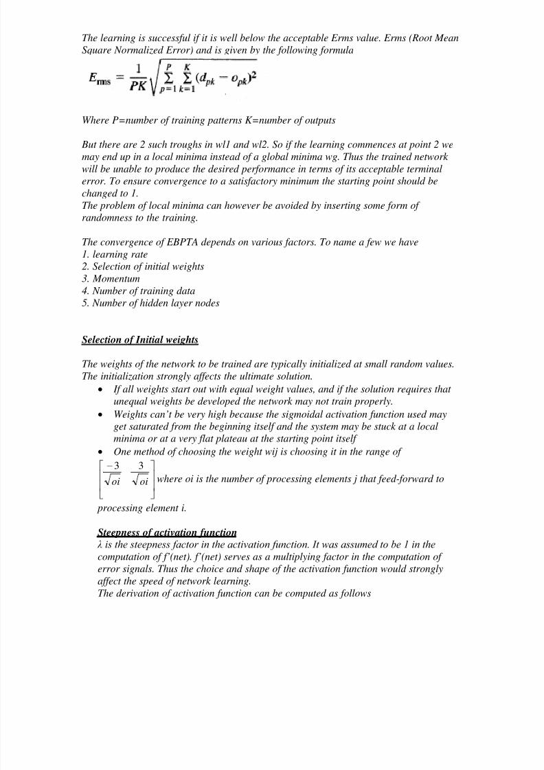
The learning is successful if it is well below the acceptable Erms value. Erms (Root Mean

Square Normalized Error) and is given by the following formula

Where P=number of training patterns K=number of outputs

But there are 2 such troughs in wl1 and wl2. So if the learning commences at point 2 we

may end up in a local minima instead of a global minima wg. Thus the trained network

will be unable to produce the desired performance in terms of its acceptable terminal

error. To ensure convergence to a satisfactory minimum the starting point should be

changed to 1.

The problem of local minima can however be avoided by inserting some form of

randomness to the training.

The convergence of EBPTA depends on various factors. To name a few we have

1. learning rate

2. Selection of initial weights3. Momentum

4. Number of training data

5. Number of hidden layer nodes

Selection of Initial weights

The weights of the network to be trained are typically initialized at small random values.

The initialization strongly affects the ultimate solution.

• If all weights start out with equal weight values, and if the solution requires that

unequal weights be developed the network may not train properly.• Weights can’t be very high because the sigmoidal activation function used may

get saturated from the beginning itself and the system may be stuck at a local

minima or at a very flat plateau at the starting point itself

• One method of choosing the weight wij is choosing it in the range of

−

oioi

33

where oi is the number of processing elements j that feed-forward to

processing element i.

λ is the steepness factor in the activation function. It was assumed to be 1 in the

computation of f’(net). f’(net) serves as a multiplying factor in the computation of

error signals. Thus the choice and shape of the activation function would strongly

affect the speed of network learning.

Steepness of activation function

The derivation of activation function can be computed as follows



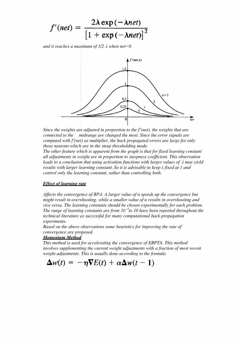
and it reaches a maximum of 1/2 λ when net=0.

Since the weights are adjusted in proportion to the f’(net), the weights that are

connected to the midrange are changed the most. Since the error signals are

computed with f’(net) as multiplier, the back propagated errors are large for only

those neurons which are in the steep thresholding mode.

The other feature which is apparent from the graph is that for fixed learning constant

all adjustments in weight are in proportion to steepness coefficient. This observation

leads to a conclusion that using activation functions with larger values of λ may yield

results with larger learning constant. So it is advisable to keep λ fixed at 1 and

control only the learning constant, rather than controlling both.

Effect of learning rate

Affects the convergence of BPA. A larger value of α speeds up the convergence but

might result in overshooting, while a smaller value of α results in overshooting and

vice versa. The learning constants should be chosen experimentally for each problem.

The range of learning constants are from 10-3

Based on the above observations some heuristics for improving the rate of

convergence are proposed.

to 10 have been reported throughout the

technical literature as successful for many computational back-propagation

experiments.

This method is used for accelerating the convergence of EBPTA. This method

involves supplementing the current weight adjustments with a fraction of most recent

weight adjustments. This is usually done according to the formula

Momentum Method



where t and t-1 represents the current and most recent training step respectively and

a is user-selected positive momentum constant. This second term is called as

momentum term. For N steps using momentum method, the current weight is

expressed as

Typically a is choosen between 0.1 and 0.8.

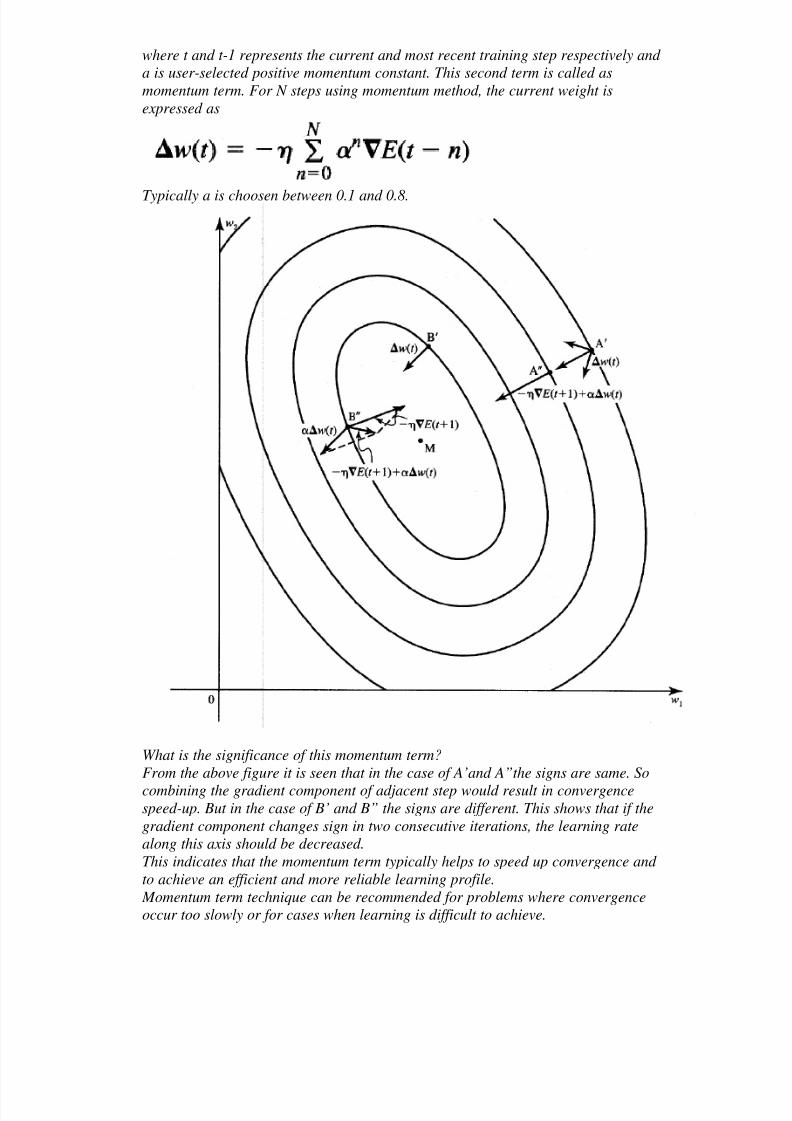
What is the significance of this momentum term?

From the above figure it is seen that in the case of A’and A”the signs are same. So

combining the gradient component of adjacent step would result in convergencespeed-up. But in the case of B’ and B” the signs are different. This shows that if the

gradient component changes sign in two consecutive iterations, the learning rate

along this axis should be decreased.

This indicates that the momentum term typically helps to speed up convergence and

to achieve an efficient and more reliable learning profile.

Momentum term technique can be recommended for problems where convergence

occur too slowly or for cases when learning is difficult to achieve.



Network architecture versus data representation

Starting from a simple case of single hidden layer the number of input nodes are

determined by the dimension, size of the input vector to be classified, generalized or

associated with a certain output quantity.

The input vector size corresponds to the number of inputs to be classified, generalized

or associated with a certain output quantity.

In planar images, size of input vector is sometimes made equal to the total number of pixels in the evaluated images.

The conditions for selecting the number of output neurons depends on the type of

neural processing. In the case of auto-associator which associates the distorted input

vector with undistorted class prototype then we have I=K.

In the case of classifier the number of output neurons are equal to the number of

classes.

Necessary number of Hidden neurons

The number of Hidden neurons depends on the dimension n of the input vector and on

the number of separable regions in n-dimensional input space.

Documents

Error Back Propagation Algorithm