Belief Propagation convergence in networksyuksel/BeliefPropStabCLJ.pdf · Belief Propagation convergence in ... haviour in networks containing cyclic paths is not fully understood

Belief Propagation convergence in networks:

April 6, 2009

Lisa Farnell, Jessica Havelock, and Claudette Yungwirth

Supervisor: Professor Serdar Yuksel

1

1 ABSTRACT

The belief propagation algorithm is an algorithm which attempts to drawconclusions from a network based off of limited information. In this project,we examine the algorithm in detail, analyzing its behaviour as certain in-put parameters are varied. Particularly, we are interested in the algorithm’sconvergence behaviours. This project aims to answer the questions: ”Whenwill the belief propagation algorithm converge to yield inferred results?” and”When will these inferred results be correct?”. The properties of the be-lief propagation algorithm are not fully understood in loopy systems. Ourresearch allows the use of the algorithm to be extended and applied to cer-tain loopy networks. This is accomplished by understanding the algorithm’sspecific convergence properties.

First we analyzed an area of the algorithm that is currently well understoodin order to gain comprehension of its processes. This consisted of analyzingthe algorithm’s performance under Markov Chain and Tree-Structured net-works as other parameters are altered while the network structures remainconstant. MATLAB simulations were then created to confirm convergenceas found in initial research.

Secondly, our analysis was extended to loopy networks, meaning those con-taining cycles. The algorithm’s behaviour in loopy networks is quite different.In order to understand when the algorithm will converge, we’ve developed aprocedure which can be applied to all loopy networks, yielding areas wherethe belief propagation algorithm will converge locally. We will also identifypoints to which the algorithm can converge for a number of situations. Theresults allow the belief propagation algorithm to be used in certain loopynetworks with a greater certainty of accurate results.

1

2 ACKNOWLEDGEMENTS

We would like to thank Dr. Serdar Yuksel for his guidance, time and supportthroughout this project.

2

Contents

1 ABSTRACT 1

2 ACKNOWLEDGEMENTS 2

3 INTRODUCTION 63.1 Background Information . . . . . . . . . . . . . . . . . . . . . 63.2 Objective . . . . . . . . . . . . . . . . . . . . . . . . . . . . . 83.3 Initial Research . . . . . . . . . . . . . . . . . . . . . . . . . . 83.4 Defining Variables . . . . . . . . . . . . . . . . . . . . . . . . . 9

4 DESCRIPTION, THEORY, AND APPROACH 94.1 Message Passing in Markov Chains, Tree structures, and Loops 94.2 Analysis of Belief Convergence . . . . . . . . . . . . . . . . . . 14

5 DESIGN 145.1 Design Goal . . . . . . . . . . . . . . . . . . . . . . . . . . . . 145.2 Design: Procedure for Showing Local Convergence . . . . . . . 15

5.2.1 Constructing the Update Function T . . . . . . . . . . 155.2.2 Examining Fixed Points of T and Contractions . . . . 185.2.3 Fixed Point Argument . . . . . . . . . . . . . . . . . . 195.2.4 Contraction Argument . . . . . . . . . . . . . . . . . . 205.2.5 Linearizing . . . . . . . . . . . . . . . . . . . . . . . . 215.2.6 Norm Discussion . . . . . . . . . . . . . . . . . . . . . 21

6 RESULTS 226.1 Convergence of Markov and Tree-Structured Networks in MAT-

LAB Simulation . . . . . . . . . . . . . . . . . . . . . . . . . . 226.2 Convergence in a Fully Connected Network . . . . . . . . . . . 23

6.2.1 Determining Fixed Points . . . . . . . . . . . . . . . . 236.2.2 Showing Convergence To Fixed Points . . . . . . . . . 24

6.3 Extending Our Analysis . . . . . . . . . . . . . . . . . . . . . 26

7 DISCUSSION 27

8 CONCLUSION 288.1 Concluding Remarks . . . . . . . . . . . . . . . . . . . . . . . 288.2 Future Work . . . . . . . . . . . . . . . . . . . . . . . . . . . . 29

3

A APPENDIX - Proofs, Derivations and Long Equations 31A.1 Markov Derivation . . . . . . . . . . . . . . . . . . . . . . . . 31A.2 Tree-Structure Derivation . . . . . . . . . . . . . . . . . . . . 31

B APPENDIX - Maple code and Results 33B.1 Maple Code for the Three-Node Fully-Connected Loop . . . . 33B.2 Maple Code for the Five-Node Fully-Connected Loop . . . . . 40B.3 Summary of Fixed Points from Maple Results . . . . . . . . . 47

C APPENDIX - MATLAB Simulations and Maple analysis Code 53C.1 Markov network code . . . . . . . . . . . . . . . . . . . . . . . 53

C.1.1 Markov network code . . . . . . . . . . . . . . . . . . . 53C.1.2 Tree-Structured network code . . . . . . . . . . . . . . 56

C.2 Fully Connected graph network code . . . . . . . . . . . . . . 59

4

List of Figures

1 Interconnected network . . . . . . . . . . . . . . . . . . . . . . 92 Markov interconnected network . . . . . . . . . . . . . . . . . 103 Tree structured graph featuring both observable and unob-

servable nodes . . . . . . . . . . . . . . . . . . . . . . . . . . . 114 Tree structured graph used for analysis . . . . . . . . . . . . . 115 Simple loopy graph . . . . . . . . . . . . . . . . . . . . . . . . 126 Illustration of message passing considered when analyzing dif-

ferent nodes of a loopy network . . . . . . . . . . . . . . . . . 137 Fully-connected five-node network . . . . . . . . . . . . . . . . 178 Local contraction around a fixed point B∗. Specifically, this

is the effect of the update function T (x) in a small neighbour-hood around B∗. . . . . . . . . . . . . . . . . . . . . . . . . . 19

9 Tree node Markov Chain MATLAB simulation output . . . . . 23

5

3 INTRODUCTION

3.1 Background Information

Belief propagation algorithms are currently used in order to analyze sys-tems which are modelled by networks. Whenever graph theory can be usedto model information with nodes and connecting communications channels,the belief propagation algorithm can be used to infer information. This ismost applicable when the information of the system - or nodal beliefs of thenetwork - are limited or unclear, possibly due to noise. Such systems canbe modelled by networks that include both nodes with observable and withunobservable beliefs.

The belief propagation algorithm can be used in a vast range of networkmodelling areas. When analysis is needed for systems with limited or noisyinformation, the belief propagation algorithm can be used to infer neededinformation or to draw conclusions based on initial observed beliefs. Mod-els used in sensor networking, weather predictions, gossip algorithms, error-correcting codes, speech recognition, and many other areas make use of thebelief propagation algorithm [1][2][3].

A system that is modelled in a graph will consist of several nodes - whichcan have observable or unobservable beliefs - and connecting lines or ”paths”.During the belief propagation algorithm, observed nodes only transmit theirinformation, and do not receive information from neighbouring nodes to up-date their belief [4]. Each unobserved node is updated at each iteration basedon the information received from neighbours [5].

In graghical reptesentation of a network, a node i is a neighbour to a node jif there is a line connecting them, implying belief information can be passedalong the path from one node to the other [6]. Connecting lines betweennodes therefore indicate conditional dependence between nodes[2][1].For agiven node in a network, any node that passes information to it is consid-ered it’s parent node, while any node to which the given node passes itsinformation to is considered it’s child node.

Networks can have directed or undirected paths. In directed paths, infor-mation can only be passed in the indicated direction. For example, if node i

6

and node j are connected with a path directed from i to j, then it is impliedthat node j can receive information from node i, but node i cannot receiveinformation from node j [2]. Graphs studied within in the scope of thisproject are primarily undirected, implying that communication can occur inboth directions on any given path.

In modelled networks, each node has its own initial belief at some time, t.Given the structure of a network, each node can share this initial belief withits neighbouring nodes during the first iteration of the algorithm. Each nodewill then update its own belief based on its received information, and willpass this updated belief to its neighbours during the next iteration, at timet + 1 [1][7][8][9]. Since each node may only share data with its neighbours,information from one node may need to pass through several others beforeits information is received by a non-neighbouring node. The message passingworks in iterative steps, until each node’s belief remains constant at successiveiterations [1][7][9].

As information is being passed during an iteration of the algorithm, anode will receive the beliefs from each of its neighbours. Its belief is thenupdated. This updated belief is then passed to its neighbours in the nextiteration, while at the same time new information is received from each ofits neighbours which is used to update its belief once again. Thus, the beliefpropagation algorithm is a recursive process which continues until a node’sbelief remains constant after multiple successive iterations.

When beliefs of all nodes remain constant after a number of algorithm it-erations, the beliefs are said to have converged[1]. The idea of convergence innetworks causes certain questions to arise as the belief propagation algorithmis implemented, such as: ”Do beliefs always converge?” and ”Which networkstructures will allow for convergence?”. It is important to note that eachnode has a probability distribution describing how much it trusts its ownopinion, and how much it trusts the messages received from each of it itsneighbours. These probability distributions are utilized by a node to updateits personal belief upon the receipt of information from its neighbours.

The algorithm is currently known to converge in linear networks such asMarkov chains and tree structured networks [7], although convergence in net-

7

works with cyclic structures remains unclear. Background research indicatesthat in networks involving cycles, the algorithm does not necessarily converge[5]. Sometimes the algorithm causes the belief of a node to be an oscillationbetween two beliefs at successive iterations [10][4]. In other instances, thealgorithm has been seen to converge to an answer that is incorrect, while inothers convergence does not occur at all [4].

3.2 Objective

Our objective is to analyze the belief propagation algorithm in detail in or-der to understand its behaviour. To be more specific, our goal is to determinethe structure of networks for which the algorithm will converge. This consistsof analyzing how convergence of the algorithm behaves as network structuresand probability distributions of variables are varied. The algorithm’s be-haviour in networks containing cyclic paths is not fully understood in beliefpropagation. Due to this fact, loopy belief will be the focus this project.

3.3 Initial Research

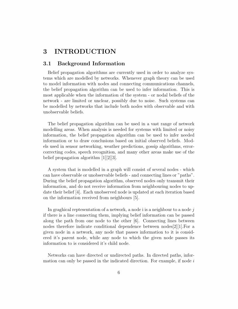
The first task of this project was to understand the belief propagationalgorithm. Dr. Yuksel provided our team with some basic examples ofapplications, and some background information about the algorithm andinterconnected networks to which it can be applied. Networks to which thealgorithm can be applied vary in complexity and structure. Figure 1, seenbelow, is an example of a complex interconnected network.

Networks are constructed of nodes and interconnecting lines. In beliefnetworks, each node has a certain belief and the lines between neighbouringnodes represent inter-nodal communication. Initially, unobservable nodesbase beliefs off the values of observable nodes. As the algorithm progresses,beliefs are communicated between nodes, and updated beliefs are generated.Convergence occurs when beliefs stay constant as updates continue to occur.

Preliminary research was conducted in order to understand the main ideasand applications behind the belief propagation algorithm. The initial generalrelationship which is further analyzed in great detail can be seen below inEquation 1.

8

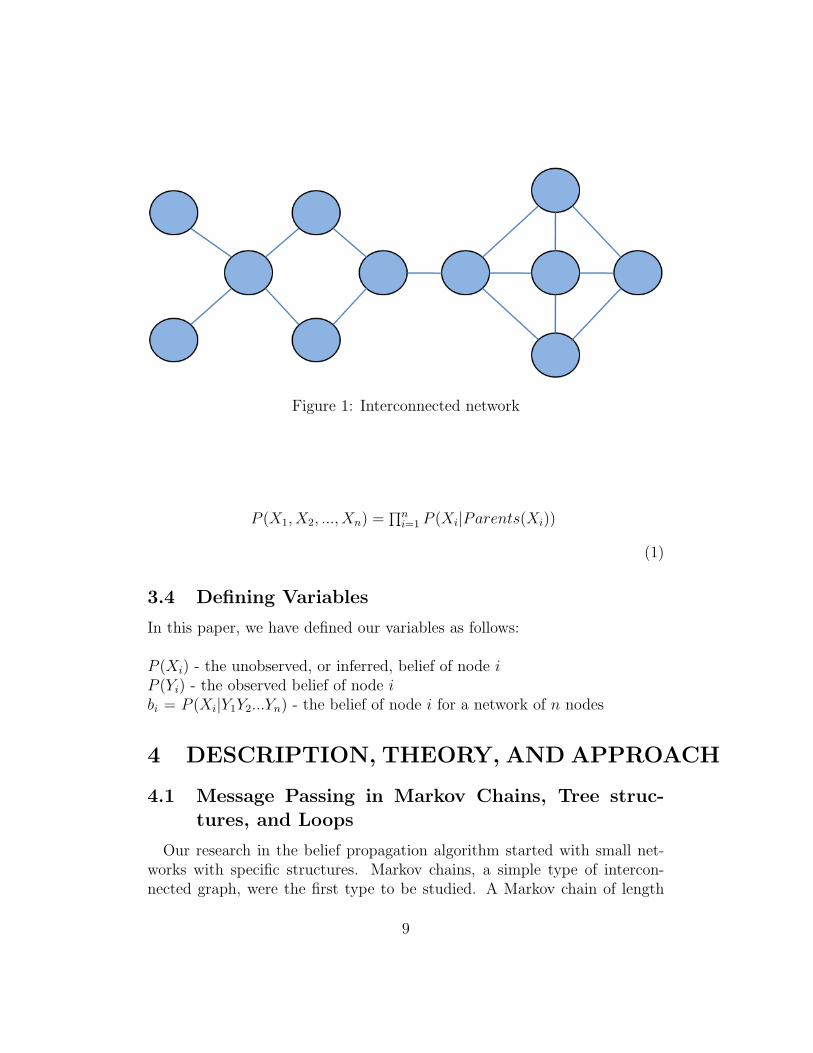
Figure 1: Interconnected network

P (X1, X2, ..., Xn) =∏n

i=1 P (Xi|Parents(Xi))

(1)

3.4 Defining Variables

In this paper, we have defined our variables as follows:

P (Xi) - the unobserved, or inferred, belief of node iP (Yi) - the observed belief of node ibi = P (Xi|Y1Y2...Yn) - the belief of node i for a network of n nodes

4 DESCRIPTION, THEORY, AND APPROACH

4.1 Message Passing in Markov Chains, Tree struc-tures, and Loops

Our research in the belief propagation algorithm started with small net-works with specific structures. Markov chains, a simple type of intercon-nected graph, were the first type to be studied. A Markov chain of length

9

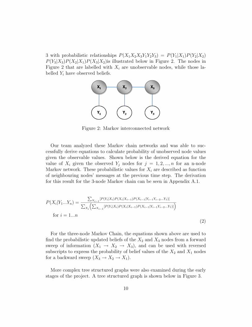
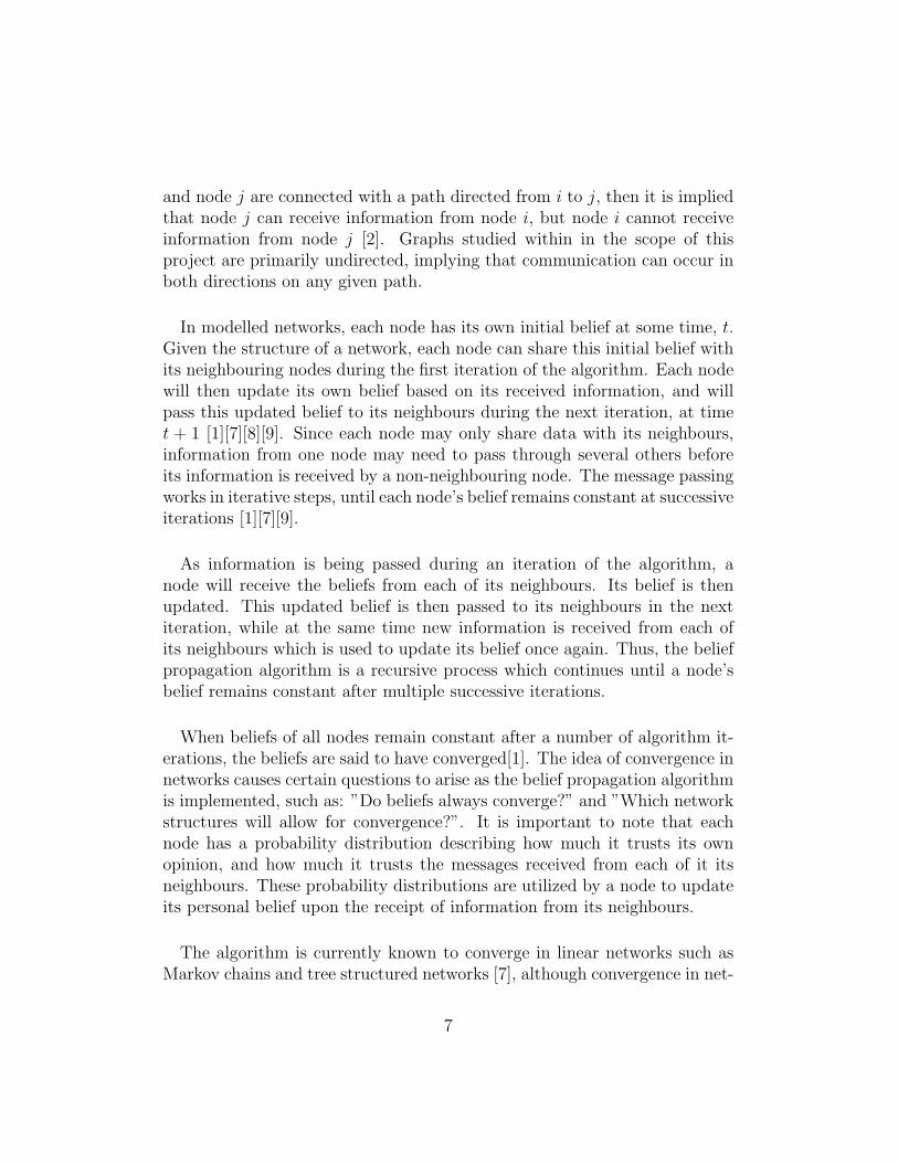
3 with probabilistic relationships P (X1X2X3Y1Y2Y3) = P (Y1|X1)P (Y2|X2)P (Y3|X3)P (X2|X1)P (X3|X2)is illustrated below in Figure 2. The nodes inFigure 2 that are labelled with Xi are unobservable nodes, while those la-belled Yi have observed beliefs.

Figure 2: Markov interconnected network

Our team analyzed these Markov chain networks and was able to suc-cessfully derive equations to calculate probability of unobserved node valuesgiven the observable values. Shown below is the derived equation for thevalue of Xi given the observed Yj nodes for j = 1, 2, ..., n for an n-nodeMarkov network. These probabilistic values for Xi are described as functionof neighbouring nodes’ messages at the previous time step. The derivationfor this result for the 3-node Markov chain can be seen in Appendix A.1.

P (Xi|Y1...Yn) =

∑Xi−1

[P (Yi|Xi)P (Xi|Xi−1)P (Xi−1|Yi−1Yi−2...Y1)]∑Xi

(∑Xi−1

[P (Yi|Xi)P (Xi|Xi−1)P (Xi−1|Yi−1Yi−2...Y1)]

)for i = 1...n

(2)

For the three-node Markov Chain, the equations shown above are used tofind the probabilistic updated beliefs of the X2 and X3 nodes from a forwardsweep of information (X1 → X2 → X3), and can be used with reversedsubscripts to express the probability of belief values of the X2 and X1 nodesfor a backward sweep (X3 → X2 → X1).

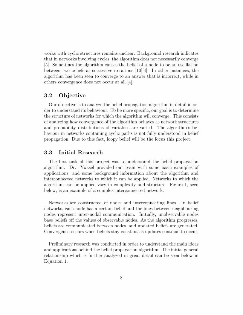
More complex tree structured graphs were also examined during the earlystages of the project. A tree structured graph is shown below in Figure 3.

10

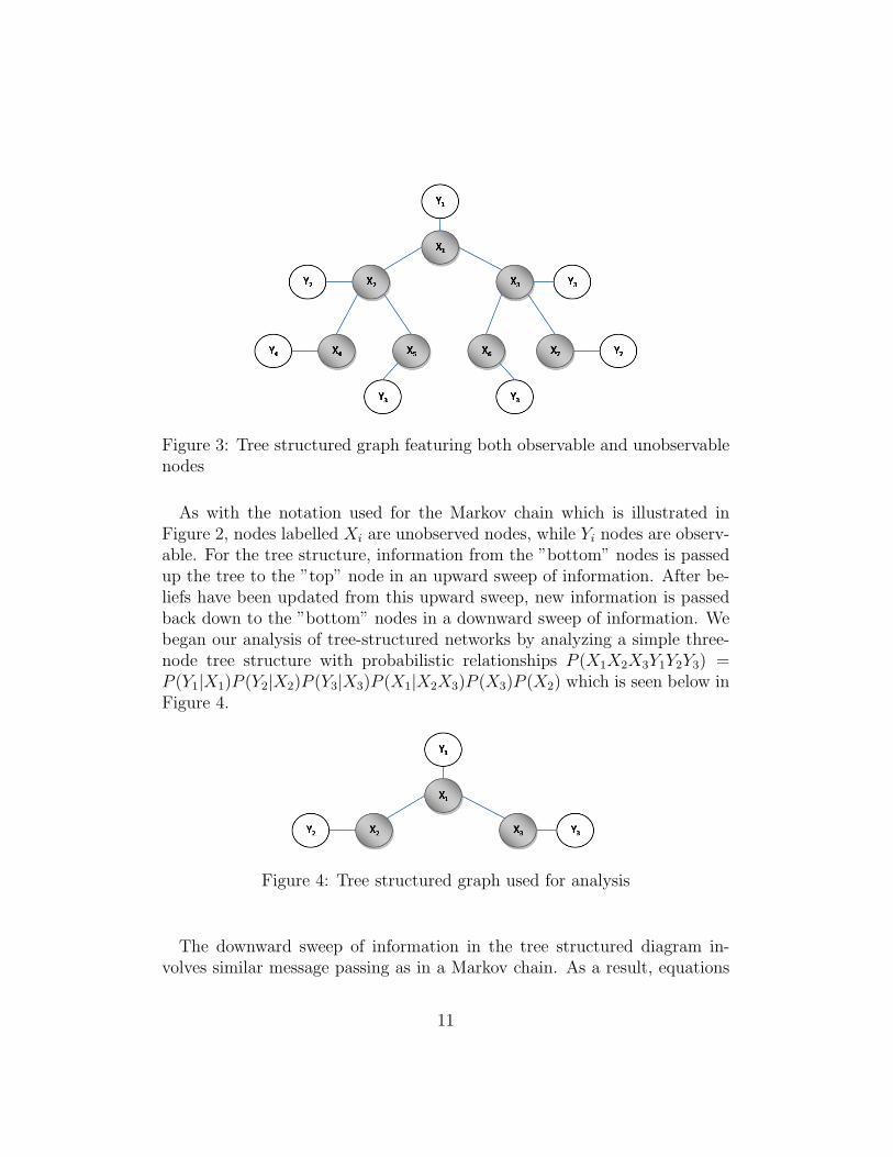
Figure 3: Tree structured graph featuring both observable and unobservablenodes

As with the notation used for the Markov chain which is illustrated inFigure 2, nodes labelled Xi are unobserved nodes, while Yi nodes are observ-able. For the tree structure, information from the ”bottom” nodes is passedup the tree to the ”top” node in an upward sweep of information. After be-liefs have been updated from this upward sweep, new information is passedback down to the ”bottom” nodes in a downward sweep of information. Webegan our analysis of tree-structured networks by analyzing a simple three-node tree structure with probabilistic relationships P (X1X2X3Y1Y2Y3) =P (Y1|X1)P (Y2|X2)P (Y3|X3)P (X1|X2X3)P (X3)P (X2) which is seen below inFigure 4.

Figure 4: Tree structured graph used for analysis

The downward sweep of information in the tree structured diagram in-volves similar message passing as in a Markov chain. As a result, equations

11

expressing the probabilistic beliefs of the Xi nodes as information is passedin a downward sweep through the ”branches” of the tree have the same formas the equations shown above for Markov chains.

An expression for an upwards sweep of a general tree-structured graph wasalso derived and can be seen below in Equation 3. This method of derivationallows for tree structured networks with n nodes to be analyzed. Note thatnodes that are ”above” the subject node are considered its parents, whilenodes that are ”below” it are considered its children. The derivation for thisequation can be seen in Appendix A.2.

P (Xi|Y1..Yn) =P (Xi|Yi)

∏c OF Xi

[∑Xj

P (Xj)P (Xj |Yj)P (Xi|Xj)

][P (Xi)]

# c OF Xi∑

Xi

P (Xi|Yi)

[P (Xi)]# c OF Xi

[∏Xj∈c OF Xi

∑Xj

P (Xi|Xj)P (Xj |Yj)P (Xj)

]where c=children

(3)

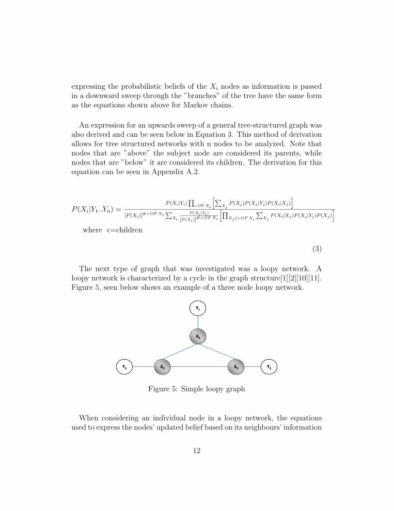
The next type of graph that was investigated was a loopy network. Aloopy network is characterized by a cycle in the graph structure[1][2][10][11].Figure 5, seen below shows an example of a three node loopy network.

Figure 5: Simple loopy graph

When considering an individual node in a loopy network, the equationsused to express the nodes’ updated belief based on its neighbours’ information

12

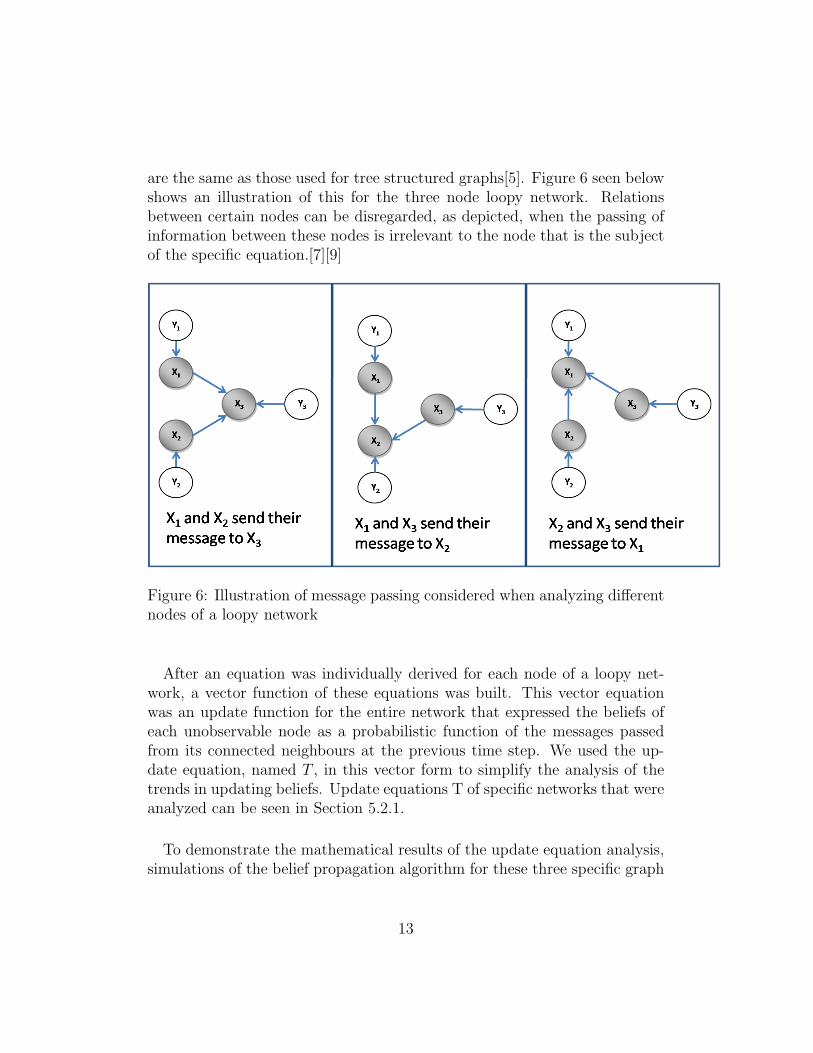
are the same as those used for tree structured graphs[5]. Figure 6 seen belowshows an illustration of this for the three node loopy network. Relationsbetween certain nodes can be disregarded, as depicted, when the passing ofinformation between these nodes is irrelevant to the node that is the subjectof the specific equation.[7][9]

Figure 6: Illustration of message passing considered when analyzing differentnodes of a loopy network

After an equation was individually derived for each node of a loopy net-work, a vector function of these equations was built. This vector equationwas an update function for the entire network that expressed the beliefs ofeach unobservable node as a probabilistic function of the messages passedfrom its connected neighbours at the previous time step. We used the up-date equation, named T , in this vector form to simplify the analysis of thetrends in updating beliefs. Update equations T of specific networks that wereanalyzed can be seen in Section 5.2.1.

To demonstrate the mathematical results of the update equation analysis,simulations of the belief propagation algorithm for these three specific graph

13

structures were created using MATLAB. A description of these simulationsand their results can be found in Section 6.

4.2 Analysis of Belief Convergence

Graphs with Markov chain or tree structures have been previously shownto converge under the belief propagation algorithm [8][7], and can intuitivelybe realized when considering how information is passed within these graphs.In both of these structures, sweeps of information in opposing directions willcause information from all nodes to be passed to every other node, and allowfor belief updates to occur with a complete set of neighbouring information.For both of these graph structures, the probabilistic beliefs of the unobserv-able nodes remain constant after a finite number of algorithm iterations.

Loopy networks have a more complicated structure than Markov chainsand tree networks; the issue of double-counting arises. Double countingoccurs when a node receives information from another node from two differentpaths. In the case of the network depicted in Figure 5 above, node X1 willreceive information from X3 that is passed directly. Node X1 will also receiveinformation from X2 that has previously been influenced by X3’s information.In this way, the information fromX3 will be sent toX1 via two different paths.

The effects of double counting on convergence were investigated by con-sidering the update function, T, of a loopy network. A fixed point was foundmathematically by solving the vector equation shown below. T was thenlinearized around this fixed point and analyzed for beliefs in a small neigh-bourhood around the fixed point. The creation and analysis of the updatefunction further is discussed in Sections 5.2.1 and 6.2.2.

(Bt) = T (Bt−1)

5 DESIGN

5.1 Design Goal

Our goal for our design is to construct a procedure to determine whena simple loopy network will converge to a belief under specific conditions.

14

These conditions will possibly restrict the following: communication betweennodes, how much one node’s belief depends on another’s belief, ie P (X1|X2),the accuracy of initial conditions, the distribution of the beliefs and possibleothers.

5.2 Design: Procedure for Showing Local Convergence

5.2.1 Constructing the Update Function T

Our designed procedure begins with the construction of a vector updatefunction which we call T. In order to analyze the methodology behind theconstruction of T, we first looked at a specific loopy network. This net-work is the simple three-node loop depicted in Figure 5. The transformationfunction, T, for this loopy network is seen below in Equation 4.

T (B) =

b11[∑1

i=0P (Y2)bi

2P (X1|X2=i)][∑1

j=0P (Y3)bj

3P (X1|X3=j)

][P (X1)]2

∑1

k=0

bk1

[P (X1=k)]2[∑1

l=0P (X1=k|X2=l)bl

2P (X2=l)][∑1

m=0P (X1=k|X3=m)bm

3 P (X3=m)]

b12[∑1

i=0P (Y1)bi

1P (X2|X1=i)][∑1

j=0P (Y3)bj

3P (X2|X3=j)

][P (X2)]2

∑1

k=0

bk2

[P (X2=k)]2[∑1

l=0P (X2=k|X1=l)bl

1P (X1=l)][∑1

m=0P (X2=k|X3=m)bm

3 P (X3=m)]

b13[∑1

i=0P (Y2)bi

2P (X3|X2=i)][∑1

j=0P (Y1)bj

1P (X3|X1=j)

][P (X3)]2

∑1

k=0

bk3

[P (X3=k)]2[∑1

l=0P (X3=k|X2=l)bl

2P (X2=l)][∑1

m=0P (X3=k|X1=m)bm

1 P (X1=m)]

(4)

This function was derived from the update equations for a tree structuredgraph that was determined in the first half of the project. Due to the natureof message passing involving only neighbouring nodes, the conditional prob-ability P (X1|Y1, Y2, Y3) found for the tree-structured network seen in Figure4 is also the first entry of the update function for the three-node loopy graphseen in Figure 5. This reasoning is also illustrated in Figure 6 as describedearlier. The transformation function T will be the updating function for allunobserved nodes at time t, where its input parameters will be the beliefs at

15

time t− 1. The equation from which the T-vector was created is of the formBt = TBt−1, as shown in Equation 5.

b1t

b2t

b3t

= T

b1t−1

b2t−1

b3t−1

(5)

Where,Bt = the beliefs of unobserved nodes at time tBt−1=the beliefs of unobserved nodes at time t− 1T= generated transformation

Since Bi is a probability distribution of beliefs, for bi ∈ Bt, we know thatbi ∈ [0, 1] for i = 1, 2, 3. This means that for Bt ∈ R3, Bt = [b1, b2, b3]

T .More generally for a loop of size n, bi ∈ [0, 1] i = 1, 2, ..., n and bt ∈ Rn with

Bt =

b1|bn

(6)

The updating function T is updating the belief at nodes X1, X2, and X3

based off of each Xi’s own belief and the belief of its neighbours at time t−1.This is done simultaneously for each node in the network. This simultaneouspassing of information is illustrated in Figure 6.

In a similar manner, probabilities can be found for any structure of net-work in order to produce the network’s update function T. This analysis wasextended to the fully-connected five-node network which is illustrated belowin Figure 7.

16

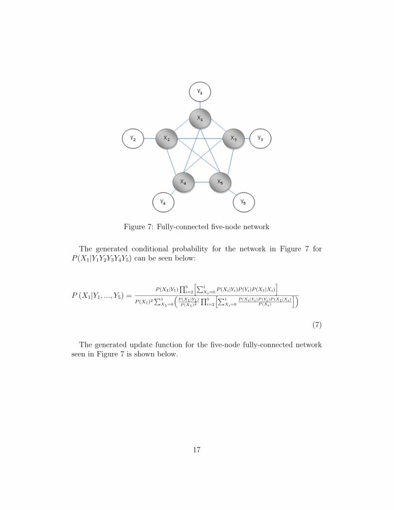
Figure 7: Fully-connected five-node network

The generated conditional probability for the network in Figure 7 forP (X1|Y1Y2Y3Y4Y5) can be seen below:

P (X1|Y1, ..., Y5) =P (X1|Y1)

∏5

i=2

[∑1

Xi=0P (Xi|Yi)P (Yi)P (X1|Xi)

]P (X1)2

∑1

X1=0

(P (X1|Y1)

P (X1)2

∏5

i=2

[∑1

Xi=0

P (Xi|Yi)P (Yi)P (X1|Xi)

P (Xi)

])

(7)

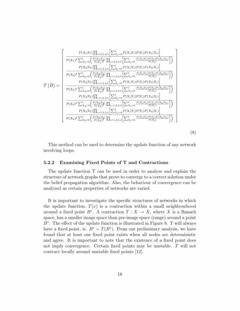
The generated update function for the five-node fully-connected networkseen in Figure 7 is shown below.

17

T (B) =

P (X1|Y1)∏

i=2,3,4,5

[∑1


]P (X1)2

∑1

X1=0

(P (X1|Y1)

P (X1)2

∏i=2,3,4,5

[∑1

Xi=0


P (Xi)

])P (X2|Y2)

∏i=1,3,4,5

[∑1


]P (X2)2

∑1

X2=0

(P (X2|Y2)

P (X2)2

∏i=1,3,4,5

[∑1

Xi=0


P (Xi)

])P (X3|Y3)

∏i=1,2,4,5

[∑1


]P (X3)2

∑1

X3=0

(P (X3|Y3)

P (X3)2

∏i=1,2,4,5

[∑1

Xi=0


P (Xi)

])P (X4|Y4)

∏i=1,2,3,5

[∑1


]P (X4)2

∑1

X4=0

(P (X4|Y4)

P (X4)2

∏i=1,2,3,5

[∑1

Xi=0


P (Xi)

])P (X5|Y5)

∏i=1,2,3,4

[∑1


]P (X5)2

∑1

X5=0

(P (X5|Y5)

P (X5)2

∏i=1,2,3,4

[∑1

Xi=0


P (Xi)

])

(8)

This method can be used to determine the update function of any networkinvolving loops.

5.2.2 Examining Fixed Points of T and Contractions

The update function T can be used in order to analyze and explain thestructure of network graphs that prove to converge to a correct solution underthe belief propagation algorithm. Also, the behaviour of convergence can beanalyzed as certain properties of networks are varied.

It is important to investigate the specific structures of networks in whichthe update function, T (x) is a contraction within a small neighbourhoodaround a fixed point B∗. A contraction T : X → X, where X is a Banachspace, has a smaller image space than pre-image space (range) around a pointB∗. The effect of the update function is illustrated in Figure 8. T will alwayshave a fixed point, ie. B∗ = T (B∗). From our preliminary analysis, we havefound that at least one fixed point exists when all nodes are deterministicand agree. It is important to note that the existence of a fixed point doesnot imply convergence. Certain fixed points may be unstable. T will notcontract locally around unstable fixed points [12].

18

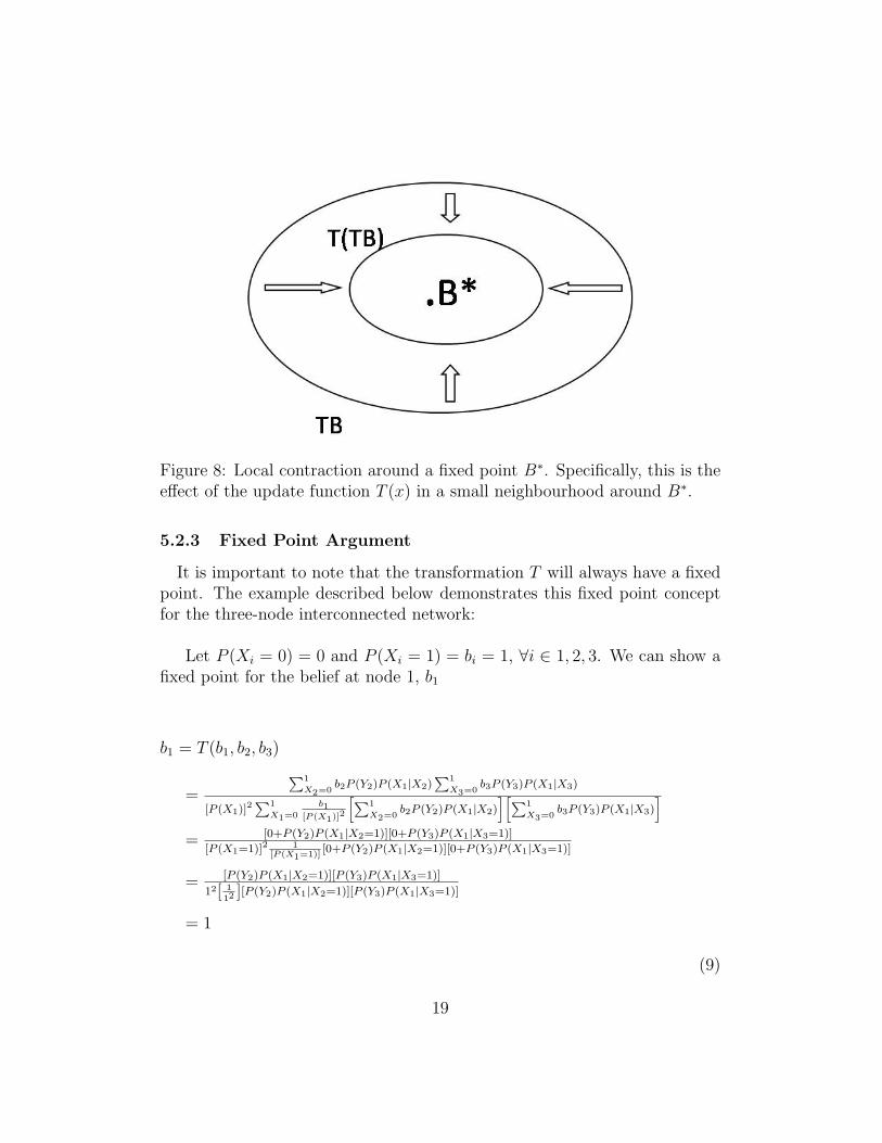
Figure 8: Local contraction around a fixed point B∗. Specifically, this is theeffect of the update function T (x) in a small neighbourhood around B∗.

5.2.3 Fixed Point Argument

It is important to note that the transformation T will always have a fixedpoint. The example described below demonstrates this fixed point conceptfor the three-node interconnected network:

Let P (Xi = 0) = 0 and P (Xi = 1) = bi = 1, ∀i ∈ 1, 2, 3. We can show afixed point for the belief at node 1, b1

b1 = T (b1, b2, b3)

=

∑1

X2=0b2P (Y2)P (X1|X2)

∑1

X3=0b3P (Y3)P (X1|X3)

[P (X1)]2∑1

X1=0

b1[P (X1)]2

[∑1

X2=0b2P (Y2)P (X1|X2)

][∑1

X3=0b3P (Y3)P (X1|X3)

]= [0+P (Y2)P (X1|X2=1)][0+P (Y3)P (X1|X3=1)]

[P (X1=1)]2 1[P (X1=1)]

[0+P (Y2)P (X1|X2=1)][0+P (Y3)P (X1|X3=1)]

= [P (Y2)P (X1|X2=1)][P (Y3)P (X1|X3=1)]

12[ 112

][P (Y2)P (X1|X2=1)][P (Y3)P (X1|X3=1)]

= 1

(9)

19

Similarly, we can show that bi = P (Xi = 1) = 1, and P (Xi = 0) =1− bi = 0, ∀i ≤ n ∈ [2, 3]

This implies that Bt = TBt−1, indicating that [1,1,1] is a fixed point. Wewill later show the existence of other fixed points.

5.2.4 Contraction Argument

Banach’s Fixed Point Theorem states that, in general, within a com-plete metric space, if T : X −→ X is a contraction and if there existsa B ∈ X such that T (B∗) = B∗, then T n(B) will converge to B∗ asn −→ ∞. That is for all B ∈ [0, 1]n, the sequence of iterates of T givenby (B, TB, T (T (B)), T (T (T (B))), .....) converges to the point B∗ within aBanach space [12].

More precisely,If B ∈ {x : ||x−B∗|| ≤ δ}, where B∗ is a fixed pointand if ||T (B)− T (B∗)|| ≤ ρ||B −B∗||, for some 0 ≤ ρ < 1Then T is a contraction and [T n(B)]converge to B∗.

Proof:

Let T be a contraction,where B∗ = T (B∗) and ρ ≤ 1so

||T (B)− T (B∗) || ≤ ρ ||B −B∗ ||||T (B)−B∗ || ≤ ρ ||B −B∗ ||||T 2(B)−B∗ || ≤ ρ2 ||B −B∗ ||||T n(B)−B∗ || ≤ ρn ||B −B∗ ||Hence [T n (B)] converges to B∗

(10)

20

5.2.5 Linearizing

To analyze the contraction properties of T we will use linear approximation.If the linearized T mapping is a contraction, then this implies that T is acontraction within a small region around B∗. This method of linearizationis valid because T is both continuous and differentiable.

5.2.6 Norm Discussion

To show convergence of the belief propagation algorithm, we must showthat the T mapping is a contraction in our discrete time space. A number ofnorms can be used to investigate T, such as the L1 norm and the L∞ norm,which are described below for a vector X with entries x1, x2, x3, ... xn.

L1 norm:

‖X‖1 =∑i |xi| , i = 1, ..., n

L∞ norm:

‖X‖∞ = max(xi), i = 1, ..., n

Our investigation of the contraction properties of T will require a completenormed space. We will consider Rn and two norms, L∞ norm and L1 whichare seen above. Under both of these norms Rn is a complete space. Thismeans that Banach’s fixed point theorem holds. For the purposes of ouranalysis, we will only look at these two norms. It easy to see that our analysisand results hold under the general Lp norm for any positive integer p. Ouranalysis can be extended to include all Lp norms because all possible beliefvalues are positive and less than one. So, our restriction to the two statednorms is without loss of generality. The general Lp norm is seen below.

21

Lp norm

‖X‖p = (∑i |xi|p)1/p

, i = 1, ..., n

6 RESULTS

(ALL MATLAB CODE IS CONTAINED IN APPENDIX C)

In this section we will present our proof of convergence and existence offixed points. Results are from mathematical analysis using pencil and paper,Maple and three MATLAB simulations, one for each analyzed network (aMarkov network, a tree network and a fully connected network).

6.1 Convergence of Markov and Tree-Structured Net-works in MATLAB Simulation

In both the Markov model and the tree structured networks, a computersimulation was created using MATLAB in order to test the algorithm andgenerated equations as well as to confirm analytical results. These simu-lations provided a more thorough understanding of the algorithm’s processof updating beliefs under different structures that were known to converge.This information assisted in formulating the approach for analysis whichwas used in the design portion of our project. The computer simulationsconfirmed that the algorithm converged to the correct answer in both theMarkov structured network and the tree structured network.

An example of the output values from the Markov model simulation isdisplayed in section Equation 9. The output shows that this Markov chainconverges after nine iterations. For this simulation, our network was setrwith the following parameters: P (Xi = 1) = 0.5, P (Xi = k|Y i = k) = 0.75and initial beliefs P (Xi = k|Y i = k) = 0.75. Also, Y -values were randomlygenerated with the use of MATLAB.

22

Figure 9: Tree node Markov Chain MATLAB simulation output

6.2 Convergence in a Fully Connected Network

In this subsection we will discuss the process of finding fixed points andthe properties of convergence around such fixed points for a fully connectednetwork. It should be noted that although other structures were not ana-lyzed in this report this analysis can be extended to include various networkstructures.

6.2.1 Determining Fixed Points

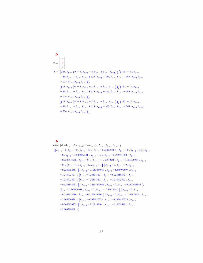
The MATLAB simulation for the fully connected network was used in orderto determine if any fixed points exist under the update function at specificparameterizations. The simulation was successful in finding fixed points butthe algorithm tended to converge on the outer regions (when the belief ofeach node is zero or one). To further our analysis, it became necessary tofind other, non-trivial fixed points. To solve this problem the beliefs weremanually initialized. The system of equations resulting from B = TB, whereB is the belief vector and T is the transformation, was solved under differentparameterizations using Maple. A summary of fixed point results can alsobe seen in Appendix B.3.

23

6.2.2 Showing Convergence To Fixed Points

The next step in our procedure is to show that T converges in a smallneighbourhood around the determined fixed point B∗. Fixed points werefound by solving B = TB with the aid of Maple software, and T was thentested for local convergence by setting initial beliefs close to the fixed point.It was found that there could be many points to which the algorithm suc-cessfully converges under a given parameterization of input variables. Inaddition, many fixed points were found that could only be reached if theywere set as the initial network belief. This implied that the algorithm doesnot necessarily converge locally around fixed points, which led to a closerlook at the contraction properties of T around various fixed points.

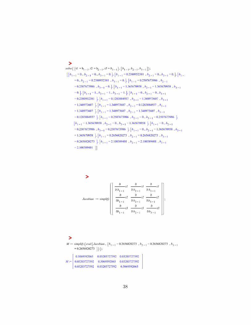
Using the linear approximation of T around the fixed points, we wereable to further examine the update function’s contraction properties aroundspecific fixed points. An example of a fixed point in the three-node fullyconnected loop, as found from the procedure explained in section 6.2.1 canbe seen below. In this case, T is a contraction within a close region of thefixed point.

Let there be three nodes, in a fully connected network, and let B∗ be thefixed point.

B∗ =

0.26568202730.26568202730.2656820273

(11)

With the help of Maple we found the Jacobian of T evaluated at B∗. Forthis particular example, the Jacobian evaluated at B∗ is given by:

24

0.50695920650 0.03203727592 0.032037275920.03203727592 0.50695920650 0.032037275920.03203727592 0.03203727592 0.50695920650

(12)

A proof of this contraction property for the example stated above can beseen below:

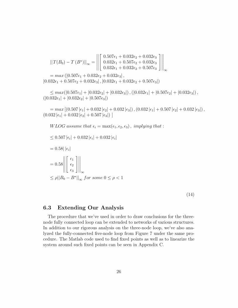
Proof of contraction property ‖T (Bo)− T (B∗)‖ ≤ ρ ‖Bo −B∗‖ under L1

norm, for fixed B∗ and initial belief vector B0 = B∗ + [ε1, ε2, ε3]T

‖T (B0)− T (B∗)‖1 =

∥∥∥∥∥∥∥ 0.507ε1 + 0.032ε2 + 0.032ε3

0.032ε1 + 0.507ε2 + 0.032ε30.032ε1 + 0.032ε2 + 0.507ε3

∥∥∥∥∥∥∥1

= |0.507ε1 + 0.032ε2 + 0.032ε3|+|0.032ε1 + 0.507ε2 + 0.032ε3|+|0.032ε1 + 0.032ε2 + 0.507ε3|

≤ |0.507ε1| + |0.032ε2| + |0.032ε3| + |0.032ε1| + |0.507ε2| + |0.032ε3| +|0.032ε1|+ |0.032ε2|+ |0.507ε3|

= 0.507 |ε1| + 0.032 |ε2| + 0.032 |ε3| + 0.032 |ε1| + 0.507 |ε2| + 0.032 |ε3| +0.032 |ε1|+ 0.032 |ε2|+ 0.507 |ε3|

≤ 0.58 |ε1|+ 0.58 |ε2|+ 0.58 |ε3|

= 0.58 (|ε1|+ |ε2|+ |ε3|)

= 0.58

∣∣∣∣∣∣∣∣∣∣∣∣∣∣ ε1ε2ε3

∣∣∣∣∣∣∣∣∣∣∣∣∣∣1

≤ ρ||B0 −B∗||1 for some 0 ≤ ρ < 1

(13)

This shows that T is a contraction within a small region of the fixed point.Thois is also true for the L∞ norm as seen below.

25

||T (B0)− T (B∗)||∞ =

∣∣∣∣∣∣∣∣∣∣∣∣∣∣ 0.507ε1 + 0.032ε2 + 0.032ε3

0.032ε1 + 0.507ε2 + 0.032ε30.032ε1 + 0.032ε2 + 0.507ε3

∣∣∣∣∣∣∣∣∣∣∣∣∣∣∞

= max (|0.507ε1 + 0.032ε2 + 0.032ε3| ,|0.032ε1 + 0.507ε2 + 0.032ε3| , |0.032ε1 + 0.032ε2 + 0.507ε3|)

≤ max(|0.507ε1|+ |0.032ε2|+ |0.032ε3|) , (|0.032ε1|+ |0.507ε2|+ |0.032ε3|) ,(|0.032ε1|+ |0.032ε2|+ |0.507ε3|)

= max [(0.507 |ε1|+ 0.032 |ε2|+ 0.032 |ε3|) , (0.032 |ε1|+ 0.507 |ε2|+ 0.032 |ε3|) ,(0.032 |ε1|+ 0.032 |ε2|+ 0.507 |ε3|) ]

WLOG assume that εi = max(ε1, ε2, ε3) , implying that :

≤ 0.507 |εi|+ 0.032 |εi|+ 0.032 |εi|

= 0.58| |εi|

= 0.58

∣∣∣∣∣∣∣∣∣∣∣∣∣∣ ε1ε2ε3

∣∣∣∣∣∣∣∣∣∣∣∣∣∣∞

≤ ρ||B0 −B∗||∞ for some 0 ≤ ρ < 1

(14)

6.3 Extending Our Analysis

The procedure that we’ve used in order to draw conclusions for the three-node fully connected loop can be extended to networks of various structures.In addition to our rigorous analysis on the three-node loop, we’ve also ana-lyzed the fully-connected five-node loop from Figure 7 under the same pro-cedure. The Matlab code used to find fixed points as well as to linearize thesystem around such fixed points can be seen in Appendix C.

26

7 DISCUSSION

Over the course of our project, we created a new systematic approach foranalyzing convergence of the loopy belief propagation algorithm. The beliefpropagation algorithm was analyzed under a three-node loopy network, andthe generated method of analyzing the algorithm under loopy systems forlocal convergence proved to be successful.

The developed method consists of determining a transfer function, whichis then used to find a fixed point. The system is then linearized around afixed point and this result is used to show existence of a local contraction.The successful proof the existence of a continuous contraction can be usedto determine the amount of error allowable in initial beliefs that will allowthe algorithm to converge. This implies that given a set range of allowableerror in initial beliefs, the algorithm will converge for loopy systems.

Our research has shown that fixed beliefs are present in all loopy three-node networks, and they depend on predefined parameters. However, incertain cases, there may not exist a fixed point under which the algorithmconverges locally. A detailed table of fixed points found for loopy graphswith varying parameters (such as distributions for variables and dependenceon neighbouring beliefs) is included in Appendix B.3.

The created methodology for mathematical analysis proved to displaypromising results. Preliminary research indicated that the algorithm willalways converge under Markov chains or tree-structured networks. Gener-ated MATLAB simulations confirm convergence in these cases after a finitenumber of iterations.

These simulations utilized random number generators in order to set andvary the observations. It was then determined that the update of beliefs attime t could be modelled as a function of previous beliefs at time t− 1. Thisfunction, which was defined as a matrix T , was then used in order to findthe existence of fixed points in the system via the use of a Maple program.

In order to demonstrate local convergence, the system was linearized arounda chosen fixed point. The result was then used to prove the existence of a

27

local contraction around the fixed point under different norms. This indi-cates that the algorithm generates positive results for the loopy case given acertain level of disagreement, or error, in original beliefs.

8 CONCLUSION

8.1 Concluding Remarks

The original methodology created and analyzed in this project is used todetermine if each node will reach a conclusion -or if the belief propagationalgorithm will converge- after a finite number of iterations. We have dis-played the existence of a small neighbourhood around a fixed point wherethe algorithm will converge in loopy networks. This result, as well as themethodology that was used, has been generated independently and, to ourknowledge, has not been seen in this form in previous research papers.

To be more specific, our methodology has been proven to show the exis-tence of a continuous local contraction around a fixed point in loopy networks.

In order to obtain this result, we first needed to find a fixed point. Todo this, concepts of probability were used to determine the general form ofa transfer function when a system involves loops. This transfer functionevaluated at an arbitrary point was set to be equal to the same arbitrarypoint, and the resulting system of equations was solved in order to find afixed point of the transformation. The system was then linearized aroundthe fixed point and the result was used in order to show the existence of alocal contraction.

We have proven that the algorithm will converge in a loopy network givena small amount of error in initial probabilities. More generally, given a initialnodal beliefs within a sufficiently small range of the fixed point, the beliefpropagation algorithm will converge to a fixed point in loopy systems. Wehave also managed to successfully extend the set of models to which thealgorithm can be used to infer accurate results.

In addition to our generated method of mathematical analysis, we’ve cre-ated MATLAB simulations which experimentally confirm results that were

28

proven mathematically. The simulations were created for four networks: aMarkov chain, a tree-structure, a three node loop, and a fully-connected fivenode network. Random number generators are used to create initial beliefsin the simulations for the Markov chain and the tree structure. In each case,as these simulations are run multiple times with varying initial beliefs, theprogram illustrates convergence.

In simulations for the three node loop and fully connected five node net-work, initial beliefs are set to be within a small neighbourhood of generatedfixed points. Again, the simulations confirm the results seen from our math-ematical methodology as convergence occurs in these cases as well.

8.2 Future Work

For networks providing update functions with fixed points, it is not alwaysthe case that there exists a contraction around such fixed points. However,the demonstration of the update function, T , being a contraction within alocal neighbourhood of an example fixed point, as shown in Section 6 showsthat convergence of the belief propagation algorithm can indeed occur ingraphs with loopy structures. Further research in this area could be per-formed in order to examine the initial parameterization of variables thatwould result in fixed points to which beliefs in local neighbourhoods willalways converge. Investigation into the size and boundaries of these localneighbourhoods could also be performed.

29

References

[1] Michael Ghil Andrew W. Robertson Padhraic Smyth Alexander T. Ihler,Sergey Kirshner. Graphical models for statistical inference and dataassimilation. Physica D, 2006.

[2] Kevin P. Murphy. An introduction to graphical models. May 2001.

[3] Balaji Prabhakar Devavrat Shah Stephen Boyd, Arpita Ghosh. Gossipalgorithms: Design, analysis, and applications. 2005.

[4] William T. Freeman Yair Weiss. On the optimality of solutions of themax-product belief propagation algorithm in arbitrary graphs. Infor-mation Theory, IEEE Transactions on, 47(2):736–744, Feb 2001.

[5] Shigeru Mase Nobuyuki Taga. On the convergence of belief propagationalgorithm for stochastic networks with loops. March 2004.

[6] William T. Freeman Jonathan S. Yedidia and Yair Weiss. Understandingbelief propagation and its generalizations. 2002.

[7] Brendan J. Frey Hans-Andrea Loeliger Frank R. Kschichang. Factorgraphs and the sum-product algorithm. Transaction on InformationTheory, 47(2), Feb 2001.

[8] Alex Olshevky John N. Tsitsiklis Vincent D. Blondel, Julien M. Hen-drickx. Convergence in multiagent coordination, consensus, and flocking.Proceedings of the 44th IEEE Conference on Decision and Control, andthe European Control Conference, Dec 2005.

[9] Buyurman Baykal Muhammet Fatih Bayramoglu, Ali Ozgur Yilmaz.Sub graph approach in iterative sum-product algorithm. 2006.

[10] Michael I. Jordan Kevin P. Murphy, Yair Weiss. Loopy belief propaga-tion for approximate inference: An empirical study. 1999.

[11] Casey Boardman. Pearl’s belief propagation algorithm and loopybayesian networks. Apr 2004.

[12] Joris M. Mooij and Hilbert J. Kappen. Sufficient conditions for conver-gence of the sum-product algorithm. May 2007.

30

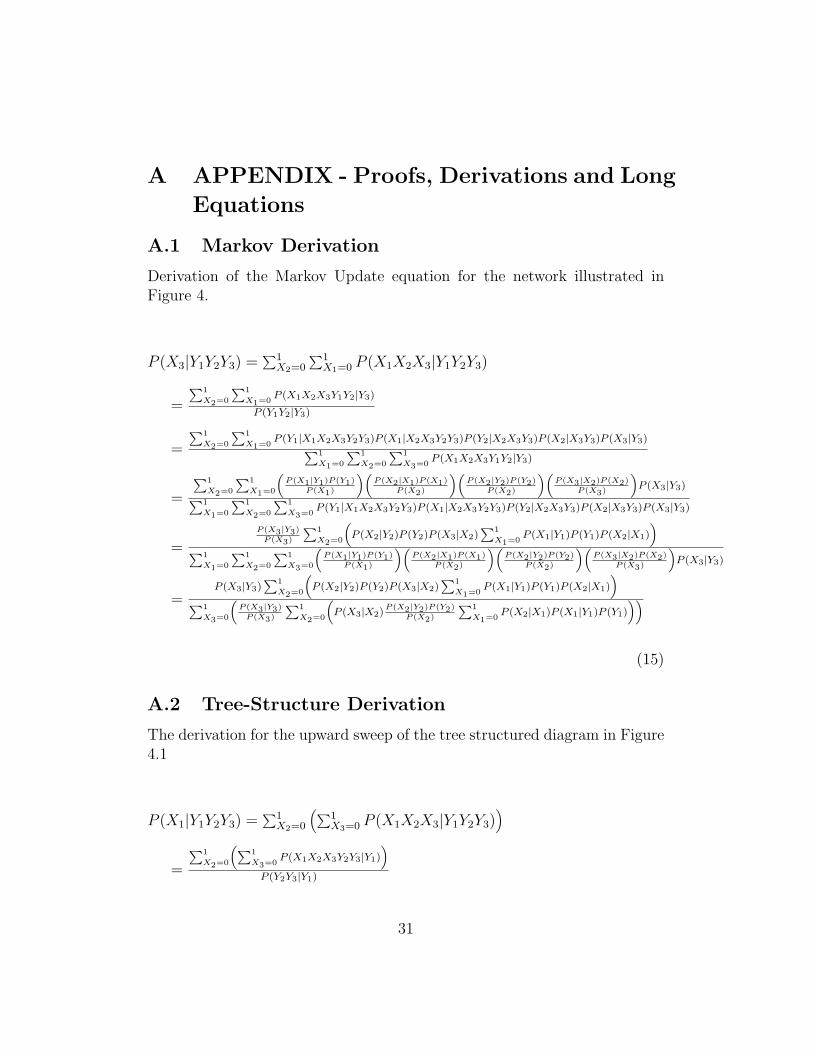
A APPENDIX - Proofs, Derivations and Long

Equations

A.1 Markov Derivation

Derivation of the Markov Update equation for the network illustrated inFigure 4.

P (X3|Y1Y2Y3) =∑1

X2=0

∑1X1=0 P (X1X2X3|Y1Y2Y3)

=

∑1

X2=0

∑1

X1=0P (X1X2X3Y1Y2|Y3)

P (Y1Y2|Y3)

=

∑1

X2=0

∑1

X1=0P (Y1|X1X2X3Y2Y3)P (X1|X2X3Y2Y3)P (Y2|X2X3Y3)P (X2|X3Y3)P (X3|Y3)∑1

X1=0

∑1

X2=0

∑1

X3=0P (X1X2X3Y1Y2|Y3)

=

∑1

X2=0

∑1

X1=0

(P (X1|Y1)P (Y1)

P (X1)

)(P (X2|X1)P (X1)

P (X2)

)(P (X2|Y2)P (Y2)

P (X2)

)(P (X3|X2)P (X2)

P (X3)

)P (X3|Y3)∑1

X1=0

∑1

X2=0

∑1

X3=0P (Y1|X1X2X3Y2Y3)P (X1|X2X3Y2Y3)P (Y2|X2X3Y3)P (X2|X3Y3)P (X3|Y3)

=P (X3|Y3)

P (X3)

∑1

X2=0

(P (X2|Y2)P (Y2)P (X3|X2)

∑1

X1=0P (X1|Y1)P (Y1)P (X2|X1)

)∑1

X1=0

∑1

X2=0

∑1

X3=0

(P (X1|Y1)P (Y1)

P (X1)

)(P (X2|X1)P (X1)

P (X2)

)(P (X2|Y2)P (Y2)

P (X2)

)(P (X3|X2)P (X2)

P (X3)

)P (X3|Y3)

=P (X3|Y3)

∑1

X2=0

(P (X2|Y2)P (Y2)P (X3|X2)

∑1

X1=0P (X1|Y1)P (Y1)P (X2|X1)

)∑1

X3=0

(P (X3|Y3)

P (X3)

∑1

X2=0

(P (X3|X2)

P (X2|Y2)P (Y2)

P (X2)

∑1

X1=0P (X2|X1)P (X1|Y1)P (Y1)

))

(15)

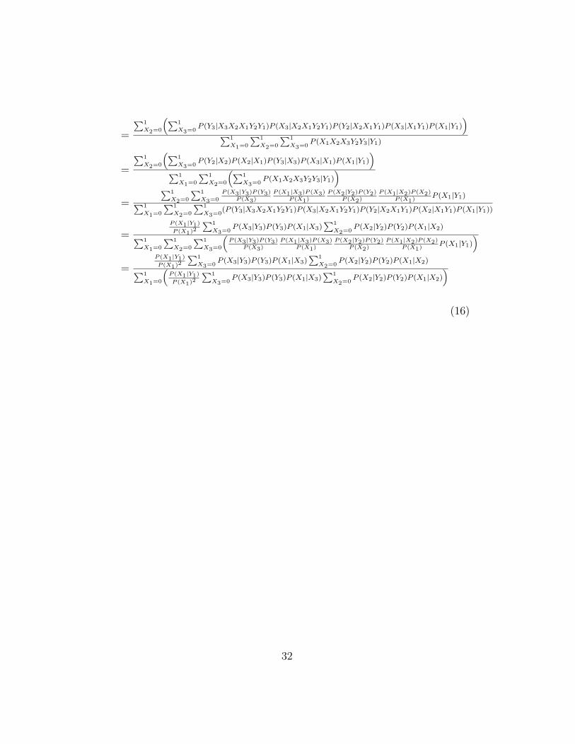
A.2 Tree-Structure Derivation

The derivation for the upward sweep of the tree structured diagram in Figure4.1

P (X1|Y1Y2Y3) =∑1

X2=0

(∑1X3=0 P (X1X2X3|Y1Y2Y3)

)

=

∑1

X2=0

(∑1

X3=0P (X1X2X3Y2Y3|Y1)

)P (Y2Y3|Y1)

31

=

∑1

X2=0

(∑1

X3=0P (Y3|X3X2X1Y2Y1)P (X3|X2X1Y2Y1)P (Y2|X2X1Y1)P (X3|X1Y1)P (X1|Y1)

)∑1

X1=0

∑1

X2=0

∑1

X3=0P (X1X2X3Y2Y3|Y1)

=

∑1

X2=0

(∑1

X3=0P (Y2|X2)P (X2|X1)P (Y3|X3)P (X3|X1)P (X1|Y1)

)∑1

X1=0

∑1

X2=0

(∑1

X3=0P (X1X2X3Y2Y3|Y1)

)=

∑1

X2=0

∑1

X3=0

P (X3|Y3)P (Y3)

P (X3)

P (X1|X3)P (X3)

P (X1)

P (X2|Y2)P (Y2)

P (X2)

P (X1|X2)P (X2)

P (X1)P (X1|Y1)∑1

X1=0

∑1

X2=0

∑1

X3=0(P (Y3|X3X2X1Y2Y1)P (X3|X2X1Y2Y1)P (Y2|X2X1Y1)P (X2|X1Y1)P (X1|Y1))

=P (X1|Y1)

P (X1)2

∑1

X3=0P (X3|Y3)P (Y3)P (X1|X3)

∑1

X2=0P (X2|Y2)P (Y2)P (X1|X2)∑1

X1=0

∑1

X2=0

∑1

X3=0

(P (X3|Y3)P (Y3)

P (X3)

P (X1|X3)P (X3)

P (X1)

P (X2|Y2)P (Y2)

P (X2)

P (X1|X2)P (X2)

P (X1)P (X1|Y1)

)=

P (X1|Y1)

P (X1)2

∑1

X3=0P (X3|Y3)P (Y3)P (X1|X3)

∑1

X2=0P (X2|Y2)P (Y2)P (X1|X2)∑1

X1=0

(P (X1|Y1)

P (X1)2

∑1

X3=0P (X3|Y3)P (Y3)P (X1|X3)

∑1

X2=0P (X2|Y2)P (Y2)P (X1|X2)

)

(16)

32

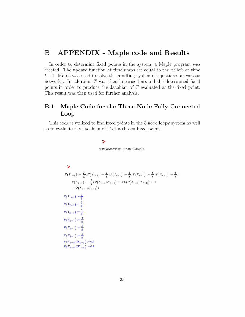
B APPENDIX - Maple code and Results

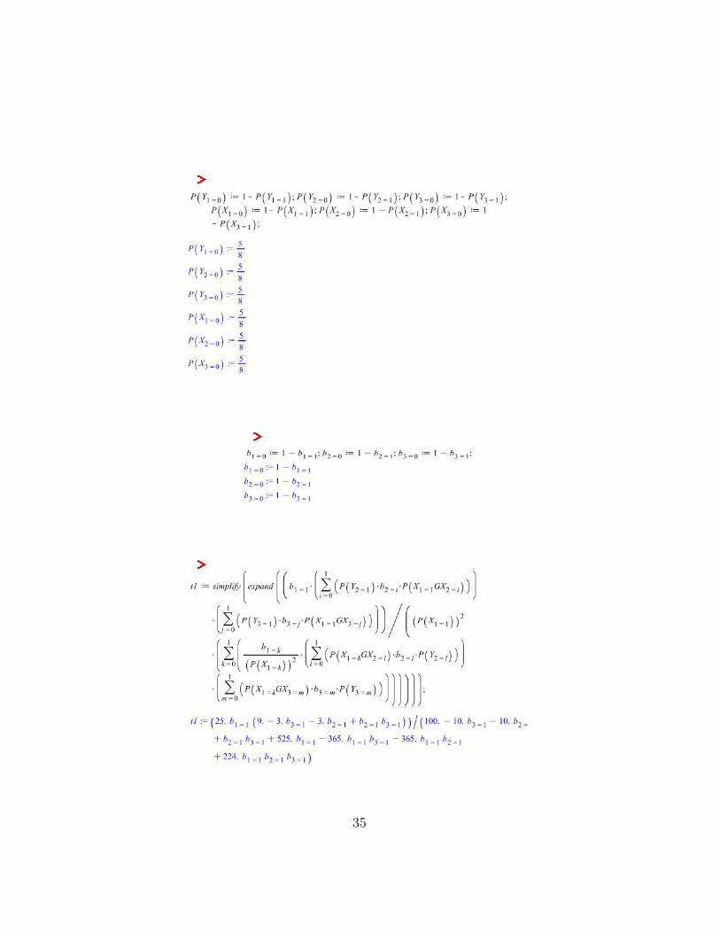
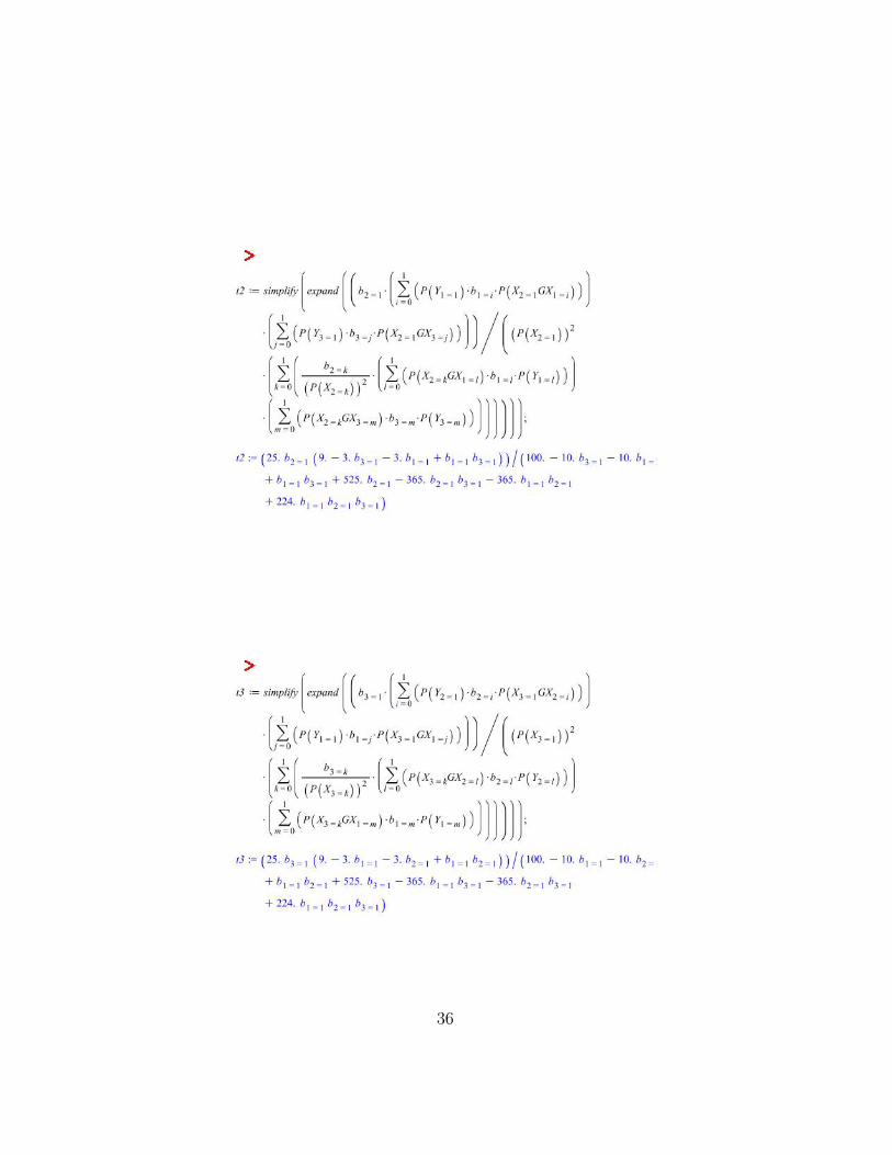
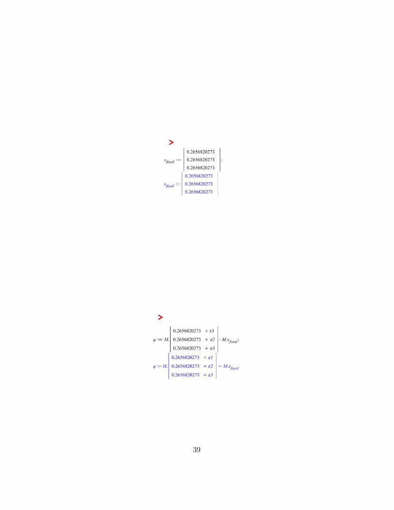
In order to determine fixed points in the system, a Maple program wascreated. The update function at time t was set equal to the beliefs at timet− 1. Maple was used to solve the resulting system of equations for variousnetworks. In addition, T was then linearized around the determined fixedpoints in order to produce the Jacobian of T evaluated at the fixed point.This result was then used for further analysis.

B.1 Maple Code for the Three-Node Fully-ConnectedLoop

This code is utilized to find fixed points in the 3 node loopy system as wellas to evaluate the Jacobian of T at a chosen fixed point.

33

34

35

36

37

38

39

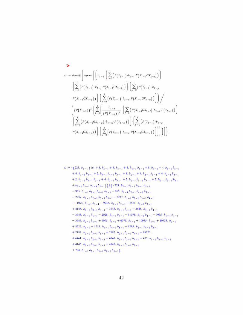
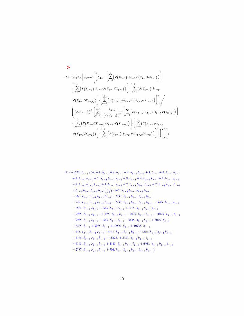
B.2 Maple Code for the Five-Node Fully-ConnectedLoop

This code is utilized to find fixed points in the 5 node fully connected sys-tem as well as to evaluate the Jacobian of T at a chosen fixed point.

Including only the real domain will eliminate solving for imaginary fixedpoints.

40

41

42

43

44

45

46

B.3 Summary of Fixed Points from Maple Results

The following tables summarize fixed points which were found for the three-node fully-connected loop as input parameters were varied.

47

48

49

50

51

52

C APPENDIX - MATLAB Simulations and

Maple analysis Code

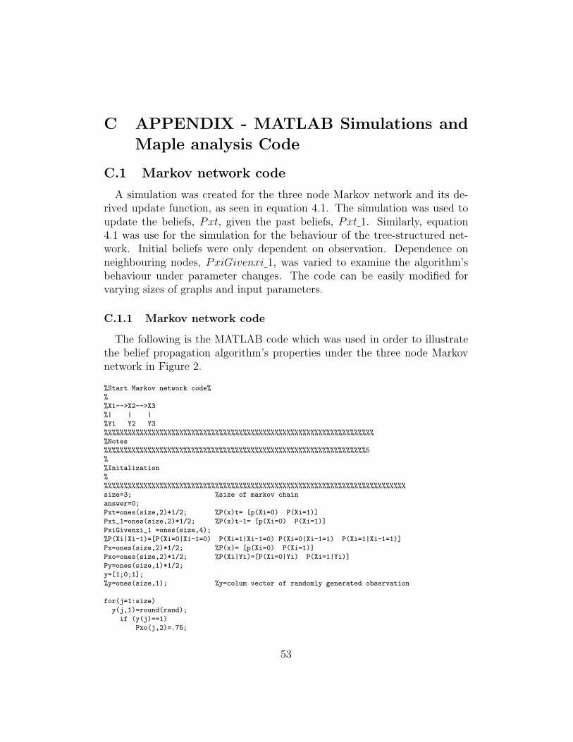
C.1 Markov network code

A simulation was created for the three node Markov network and its de-rived update function, as seen in equation 4.1. The simulation was used toupdate the beliefs, Pxt, given the past beliefs, Pxt 1. Similarly, equation4.1 was use for the simulation for the behaviour of the tree-structured net-work. Initial beliefs were only dependent on observation. Dependence onneighbouring nodes, PxiGivenxi 1, was varied to examine the algorithm’sbehaviour under parameter changes. The code can be easily modified forvarying sizes of graphs and input parameters.

C.1.1 Markov network code

The following is the MATLAB code which was used in order to illustratethe belief propagation algorithm’s properties under the three node Markovnetwork in Figure 2.

%Start Markov network code%

%

%X1-->X2-->X3

%| | |

%Y1 Y2 Y3

%%%%%%%%%%%%%%%%%%%%%%%%%%%%%%%%%%%%%%%%%%%%%%%%%%%%%%%%%%%%%%%%%%%%

%Notes

%%%%%%%%%%%%%%%%%%%%%%%%%%%%%%%%%%%%%%%%%%%%%%%%%%%%%%%%%%%%%%%%%%5

%

%Initalization

%

%%%%%%%%%%%%%%%%%%%%%%%%%%%%%%%%%%%%%%%%%%%%%%%%%%%%%%%%%%%%%%%%%%%%%%%%%%%%

size=3; %size of markov chain

answer=0;

Pxt=ones(size,2)*1/2; %P(x)t= [p(Xi=0) P(Xi=1)]

Pxt_1=ones(size,2)*1/2; %P(x)t-1= [p(Xi=0) P(Xi=1)]

PxiGivenxi_1 =ones(size,4);

%P(Xi|Xi-1)=[P(Xi=0|Xi-1=0) P(Xi=1|Xi-1=0) P(Xi=0|Xi-1=1) P(Xi=1|Xi-1=1)]

Px=ones(size,2)*1/2; %P(x)= [p(Xi=0) P(Xi=1)]

Pxo=ones(size,2)*1/2; %P(Xi|Yi)=[P(Xi=0|Yi) P(Xi=1|Yi)]

Py=ones(size,1)*1/2;

y=[1;0;1];

%y=ones(size,1); %y=colum vector of randomly generated observation

for(j=1:size)

y(j,1)=round(rand);

if (y(j)==1)

Pxo(j,2)=.75;

53

Pxo(j,1)=.25;

else

Pxo(j,1)=.75;

Pxo(j,2)=.25;

end

Pxt_1(j,2)=Pxo(j,2);

end

%%%%%%%%%%%%%%%%%%%%%%%%%%%%%%%%%%%%%%%%%%%%%%%%%%%%%%%%%%%%%%%%%%%%%%%%%%%%%%%%%%%%%%%%%%%%%%%%

%

%loop

%

%%%%%%%%%%%%%%%%%%%%%%%%%%%%%%%%%%%%%%%%%%%%%%%%%%%%%%%%%%%%%%%%%%%%%%%%%%%%%%%%%%%%%%%%%%%%%

for(k=1:10)

%%%%%%%%%%%%%%%%%%%%%%%%%%%%%%%%%%%%%%%%%%%%%%%%%%%%%%%%%%%%%%%%%%%%%%%%%%%%%%%%%%%%%%%%%%%%%%%%

%Forwards part

%%%%%%%%%%%%%%%%%%%%%%%%%%%%%%%%%%%%%%%%%%%%%%%%%%%%%%%%%%%%%%%%%%%%%%%%%%%%%%%%%%%%%%%%%%%%%

for(j=2:size)

if (round(Pxo(j,2))==round(Pxo(j-1,2)))

PxiGivenxi_1(j,1)=.75;




else





end

end

Pxt(1,2)=Pxt_1(1,2);

for(i=2:size)

top=Pxo(i,2)*(Pxt_1(i-1,1)*PxiGivenxi_1(i,4))+(Pxt_1(i-1,2)*PxiGivenxi_1(i,2));

Pyigiveny=(Py(i)*((Pxo(i,2)/Px(i,2))*((PxiGivenxi_1(i,4)*Pxt_1(i-1,2))+(PxiGivenxi_1(i,2)

*Pxt_1(i-1,1))))+((((Pxo(i,1))/Px(i,1))*((PxiGivenxi_1(i,3)*Pxt_1(i-1,2))

+(PxiGivenxi_1(i,1)*Pxt_1(i-1,1))))));

Pxt(i,2)=top/Pyigiveny;

end

%%%%%%%%%%%%%%%%%%%%%%%%%%%%%%%%%%%%%%%%%%%%%%%%%%%%%%%%%%%%%%%%%%%%%%%%%%%%%%%%%%%%

%

%update-forwards

%

%%%%%%%%%%%%%%%%%%%%%%%%%%%%%%%%%%%%%%%%%%%%%%%%%%%%%%%%%%%%%%%%%%%%%%%%%%%%%%%%%

for(j=1:size)

Pxt_1(j,2)=Pxt(j,2); %

Pxt_1(j,1)=1-Pxt(j,2); %update p(x) at t-1

if (y(j)==1) %update P(xi|yi)

Pxo(j,2)=.75;

Pxo(j,1)=.25;

else

Pxo(j,1)=.75;

Pxo(j,2)=.25;

end

end

54

%%%%%%%%%%%%%%%%%%%%%%%%%%%%%%%%%%%%%%%%%%%%%%%%%%%%%%%%%%%%%%%%%%%%%%%%%%%%%%%%%%%%%%%%%%%%%%%%

%Backwards part

%%%%%%%%%%%%%%%%%%%%%%%%%%%%%%%%%%%%%%%%%%%%%%%%%%%%%%%%%%%%%%%%%%%%%%%%%%%%%%%%%%%%%%%%%%%%%

for(j=1:size-1)

if (round(Pxo(j,2))==round(Pxo(j+1,2)))





else





end

end

Pxt(size,2)=Pxt_1(size,2);

i=size;

while(i>1)

i=i-1;

top=Pxo(i,2)*(Pxt_1(i+1,1)*PxiGivenxi_1(i,4))+(Pxt_1(i+1,2)*PxiGivenxi_1(i,2));

Pyigiveny=(Py(i)*((Pxo(i,2)/Px(i,2))*((PxiGivenxi_1(i,4)*Pxt_1(i+1,2))

+(PxiGivenxi_1(i,2)*Pxt_1(i+1,1))))+((((Pxo(i,1))/Px(i,1))

*((PxiGivenxi_1(i,3)*Pxt_1(i+1,2))+(PxiGivenxi_1(i,1)*Pxt_1(i+1,1))))));

Pxt(i,2)=top/Pyigiveny;

end

%%%%%%%%%%%%%%%%%%%%%%%%%%%%%%%%%%%%%%%%%%%%%%%%%%%%%%%%%%%%%%%%%%%%%%%%%%%%%%%%%%%%

%

%update-backwards

%

%%%%%%%%%%%%%%%%%%%%%%%%%%%%%%%%%%%%%%%%%%%%%%%%%%%%%%%%%%%%%%%%%%%%%%%%%%%%%%%%%

for(j=1:size)

Pxt_1(j,2)=Pxt(j,2); %


if (y(j)==1) %update P(xi|yi)??????

Pxo(j,2)=.75;

Pxo(j,1)=.25;

else

Pxo(j,1)=.75;

Pxo(j,2)=.25;

end

end

Pxt_1

end

y

%%%%%%%%%%%%%%%%%%%%%%%%%%%%%%%%%%%%%%%%%%%%%%%%%%%%%%%%%%%

% end Markov network code

%%%%%%%%%%%%%%%%%%%%%%%%%%%%%%%%%%%%%%%%%%%%%%%%%%%%%%%%%%%

55

C.1.2 Tree-Structured network code

The following is the MATLAB code which was used in order to illustratethe belief propagation algorithm’s properties under the tree-structured net-work seen in Figure 4.

%%%%%%%%%%%%%%%%%%%%%%%%%%%%%%%%%%%%%%%%%%%%%%%%%%%%%%%%%%%%

% start Tree network code

%%%%%%%%%%%%%%%%%%%%%%%%%%%%%%%%%%%%%%%%%%%%%%%%%%%%%%%%%%%

%Y1

% |

% X1

% / \

% X2 X2

% | |

% Y2 Y3

%%%%%%%%%%%%%%%%%%%%%%%%%%%%%%%%%%%%%%%%%%%%%%%%%%%%%%%%%%%%%%%%%%%%

%Notes

%-insert bottem and test

%

%

%

%

%%%%%%%%%%%%%%%%%%%%%%%%%%%%%%%%%%%%%%%%%%%%%%%%%%%%%%%%%%%%%%%%%%5

%

%Initalization

%

%%%%%%%%%%%%%%%%%%%%%%%%%%%%%%%%%%%%%%%%%%%%%%%%%%%%%%%%%%%%%%%%%%%%%%%%%%%%


Pxt=ones(size,2)*1/2; %P(x)t= [p(Xi=0) P(Xi=1)]

Gragh=zeros(size,size); %|0 1 1|-one is added if they are directly conected

%|1 0 0|

%|1 0 0|

Pxt_1=ones(size,2)*1/2; %P(x)t-1= [p(Xi=0) P(Xi=1)]

PxiGivenxi_1 =ones(size,4);

%P(Xi|Xi-1)= [P(Xi=0|Xi-1=0) P(Xi=1|Xi-1=0) P(Xi=0|Xi-1=1) P(Xi=1|Xi-1=1)]


Pxo=ones(size,2)*1/2; %P(Xi|Yi)=[P(Xi=0|Yi) P(Xi=1|Yi)]

Py=ones(size,1)*1/2;

%y=[1;1;0];

y=ones(size,1); %y=colum vector of randomly generated observation

top=1;

bottem=1;

for(j=1:size)

y(j,1)=round(rand);

if (y(j)==1)

Pxo(j,2)=.75;

Pxo(j,1)=.25;

else

Pxo(j,1)=.75;

Pxo(j,2)=.25;

end

Pxt_1(j,2)=Pxo(j,2);

end

56

%%%%%%%%%%%%%%%%%%%%%%%%%%%%%%%%%%%%%%%%%%%%%%%%%%%%%%%%%%%%%%%%%%%%%

%initalize gragh

%%%%%%%%%%%%%%%%%%%%%%%%%%%%%%%%%%%%%%%%%%%%%%%%%%%%%%%%%%%%%%5

Gragh=[0 1 1 0 0 0 0; 1 0 0 1 1 0 0 ;1 0 0 0 0 1 1;

0 1 0 0 0 0 0;0 1 0 0 0 0 0;0 0 1 0 0 0 0; 0 0 1 0 0 0 0];

%%%%%%%%%%%%%%%%%%%%%%%%%%%%%%%%%%%%%%%%%%%%%%%%%%%%%%%%%%%%%%%%%%%%%%%%%%%%%%%%%%%%%%%%%%%%%%%%

%going up the tree

%%%%%%%%%%%%%%%%%%%%%%%%%%%%%%%%%%%%%%%%%%%%%%%%%%%%%%%%%%%%%%%%%%%%%%%%%%%%%%%%%%%%%%%%%%%%%

%%%%%%%%%%%%%%%%%%%%%%%%%%%%%%%%%%%%%%%%%%%%%%%%%%%%%%%%%%%%%%%%%%%%%%%%%%%%%%%%%%%%%%%%%%%%%%%%

%

%loop-up(to X1)

%

%%%%%%%%%%%%%%%%%%%%%%%%%%%%%%%%%%%%%%%%%%%%%%%%%%%%%%%%%%%%%%%%%%%%%%%%%%%%%%%%%%%%%%%%%%%%%

for(k=1:10)

for(x=1:size)

test=0;

top=1;

bottemx1=1;

bottemx0=1;

for(i=1:size)

if (round(Pxo(x,2))==round(Pxo(i,2)))

PxiGivenxi_1(i,1)=.75;




else





end

if(Gragh(x,i)==1 && x<i)

top=top*(Px(i,2)/Py(i))*((Pxt_1(i,2)*PxiGivenxi_1(i,4))+(Pxt_1(i,1)*PxiGivenxi_1(i,3)));

bottemx0=bottemx0*((Px(i,1))*(PxiGivenxi_1(i,1)*Pxt_1(i,1))

+(Px(i,2))*(PxiGivenxi_1(i,2)*Pxt_1(i,2)));

bottemx1=bottemx1*((Px(i,1))*(PxiGivenxi_1(i,3)*Pxt_1(i,1))

+(Px(i,2))*(PxiGivenxi_1(i,4)*Pxt_1(i,2)));

test=1;

end

end

if (test==0)

Pxt(x,2)=Pxt_1(x,2);

else

top=Pxo(x,2)*top;

bottemx0=(Pxo(x,1)/Px(x,1)^2)*bottemx0;

bottemx1=(Pxo(x,2)/Px(x,2)^2)*bottemx1;

bottem=bottemx1+bottemx0;

Pxt(x,2)=top/bottem;

end

end

%%%%%%%%%%%%%%%%%%%%%%%%%%%%%%%%%%%%%%%%%%%%%%%%%%%%%%%%%%%%%%%%%%%%%%%%%%%%%%%%%%%%

%update-up

%%%%%%%%%%%%%%%%%%%%%%%%%%%%%%%%%%%%%%%%%%%%%%%%%%%%%%%%%%%%%%%%%%%%%%%%%%%%%%%%%

for(j=1:size)

Pxt_1(j,2)=Pxt(j,2); %

57


end

%%%%%%%%%%%%%%%%%%%%%%%%%%%%%%%%%%%%%%%%%%%%%%%%%%%%%%%%%%%%%%%%%%%%%%%%%%%%%%%%%%%%%%%%%%%%%%%%

%Going down the tree

%%%%%%%%%%%%%%%%%%%%%%%%%%%%%%%%%%%%%%%%%%%%%%%%%%%%%%%%%%%%%%%%%%%%%%%%%%%%%%%%%%%%%%%%%%%%%

%%%%%%%%%%%%%%%%%%%%%%%%%%%%%%%%%%%%%%%%%%%%%%%%%%%%%%%%%%%%%%%%%%%%%%%%%%%%%%%%%%%%%%%%%%%%%%%%

%

%loop-down

%

%%%%%%%%%%%%%%%%%%%%%%%%%%%%%%%%%%%%%%%%%%%%%%%%%%%%%%%%%%%%%%%%%%%%%%%%%%%%%%%%%%%%%%%%%%%%%

x=1;

while(x<size+1)

test=0;

top=1;

bottemx1=1;

bottemx0=1;

i=size;

while(i>0)

if (round(Pxo(x,2))==round(Pxo(i,2)))





else





end

if(Gragh(x,i)==1 && x>i)

top=Pxo(x,2)*(Px(i)/Py(i))*((Pxt_1(i,2)*PxiGivenxi_1(i,4))

+(Pxt_1(i,1)*PxiGivenxi_1(i,2)));

bottem=(Py(i)*((Pxo(x,2)/Px(x,2))*((PxiGivenxi_1(i,4)*Pxt_1(i,2))

+(PxiGivenxi_1(i,2)*Pxt_1(i,1))))

+((((Pxo(x,1))/Px(x,1))*((PxiGivenxi_1(i,3)*Pxt_1(i,2))

+(PxiGivenxi_1(i,1)*Pxt_1(i,1))))));

i=0;


else

i=i-1;

end

end

x=x+1;

end

%%%%%%%%%%%%%%%%%%%%%%%%%%%%%%%%%%%%%%%%%%%%%%%%%%%%%%%%%%%%%%%%%%%%%%%%%%%%%%%%%%%%

%

%update-down

%

%%%%%%%%%%%%%%%%%%%%%%%%%%%%%%%%%%%%%%%%%%%%%%%%%%%%%%%%%%%%%%%%%%%%%%%%%%%%%%%%%

for(j=1:size)

Pxt_1(j,2)=Pxt(j,2); %


58

if (y(j)==1) %update P(xi|yi)

Pxo(j,2)=.75;

Pxo(j,1)=.25;

else

Pxo(j,1)=.75;

Pxo(j,2)=.25;

end

end

Pxt_1

end

y

%%%%%%%%%%%%%%%%%%%%%%%%%%%%%%%%%%%%%%%%%%%%%%%%%%%%%%%%%%%

% end Tree network code

%%%%%%%%%%%%%%%%%%%%%%%%%%%%%%%%%%%%%%%%%%%%%%%%%%%%%%%%%%%

C.2 Fully Connected graph network code

The following is the MATLAB code which was used in order to illustratethe belief propagation algorithm’s properties under the fully-connected net-work seen in Figure 5.

The simulation for the fully connected network was approached in the sameway as the Markov network and the tree network, using equation - for theupdate. The major difference between the previous two simulations and thatof the fully-connected network was the method of initializing beliefs. Thiswas done manually for the fully-connected network, whereas beliefs wereautomatically initialized in the Markov and tree-structure simulations.

% Y1

% |

% X1

% / \

% X2---X2

% | |

% Y2 Y3

%%%%%%%%%%%%%%%%%%%%%%%%%%%%%%%%%%%%%%%%%%%%%%%%%%%%%%%%%%%%%%%%%%%%

%Notes

%-

%

%

%

%

%%%%%%%%%%%%%%%%%%%%%%%%%%%%%%%%%%%%%%%%%%%%%%%%%%%%%%%%%%%%%%%%%%5

%

%Initalization

%

59

%%%%%%%%%%%%%%%%%%%%%%%%%%%%%%%%%%%%%%%%%%%%%%%%%%%%%%%%%%%%%%%%%%%%%%%%%%%%


Gragh=zeros(size,size); %|0 1 1|-one is added if they are directly conected

%|1 0 1|

startpoint=.9 %|1 1 0|


Py=ones(size,1)*7/8; %P(y)= [p(Yi=0) P(Yi=1)]

y=ones(size,1); %y=colum vector of randomly generated observation

Pxt=ones(size,2)*startpoint; %P(x|Y,Y,Y)t= [p(Xi=0|Y,Y,Y) P(Xi=1|y,y,y)]

%P(x|Y,Y,Y)t-1= [p(Xi=0|y,y,y) P(Xi=1|y,y,y)]

Pxt_1=ones(size,2)*startpoint;

PxiGivenxi_1 =ones(size,4); %P(Xi|Xi-1)=|P(Xi=0|Xi-1=0) P(Xi=1|Xi-1=0) P(Xi=0|Xi-1=1) P(Xi=1|Xi-1=1)]

% |P(Xi=0|Xi-2=0) P(Xi=1|Xi-2=0) P(Xi=0|Xi-2=1) P(Xi=1|Xi-2=1)]

top=1; %top=top of update equation

bottemx0=1; %bottemx0=bottem half of denominatior where x=0

bottemx1=1; %bottemx1=bottem half of denominatior where x=1

for(j=1:size)

%y(j,1)=round(rand);

Px(j,1)=1-Px(j,2);

Pxt(j,1)=1-startpoint;

Pxt_1(j,1)=1-startpoint;

if(y(j,1)==0)

Py(j,1)=Px(j,1);

end

end

Pxt

%%%%%%%%%%%%%%%%%%%%%%%%%%%%%%%%%%%%%%%%%%%%%%%%%%%%%%%%%%%%%%%%%%%%%

%initalize gragh

%%%%%%%%%%%%%%%%%%%%%%%%%%%%%%%%%%%%%%%%%%%%%%%%%%%%%%%%%%%%%%5

Gragh=[0 1 1 1 1; 1 0 1 1 1 ;1 1 0 1 1;1 1 1 0 1;1 1 1 1 0];

%%%%%%%%%%%%%%%%%%%%%%%%%%%%%%%%%%%%%%%%%%%%%%%%%%%%%%%%%%%%%%%%%%%%%%%%%%%%%%%%%%%%%%%%%%%%%%%%

% Update P(x|x)

%%%%%%%%%%%%%%%%%%%%%%%%%%%%%%%%%%%%%%%%%%%%%%%%%%%%%%%%%%%%%%%%%%%%%%%%%%%%%%%%%%%%%%%%%%%%%

for (k=1:15)

for(x=1:size)

top=1;

bottemx1=1;

bottemx0=1;

for(i=1:size)

if (round(Pxt_1(x,2))==round(Pxt_1(i,2))) %findP(x|xi)





else





end

%%%%%%%%%%%%%%%%%%%%%%%%%%%%%%%%%%%%%%%%%%%%%%%%%%%%%%%%%%%%%%%%%%%%%%%%%%%%%%%%%%%%%%%%%%%%%%%%

60

% P(Xt|Y,Y,Y)=TP(Xt_1|Y,Y,Y)

%%%%%%%%%%%%%%%%%%%%%%%%%%%%%%%%%%%%%%%%%%%%%%%%%%%%%%%%%%%%%%%%%%%%%%%%%%%%%%%%%%%%%%%%%%%%%

if(Gragh(x,i)==1)

top=top*(Py(i))*((Pxt_1(i,2)*PxiGivenxi_1(i,4))+(Pxt_1(i,1)*PxiGivenxi_1(i,3)));

bottemx0=bottemx0*((Px(i,1))*(PxiGivenxi_1(i,1)*Pxt_1(i,1))+(Px(i,2))

*(PxiGivenxi_1(i,2)*Pxt_1(i,2)));

bottemx1=bottemx1*((Px(i,1))*(PxiGivenxi_1(i,3)*Pxt_1(i,1))+(Px(i,2))

*(PxiGivenxi_1(i,4)*Pxt_1(i,2)));

end

end

top=(Pxt(x,2))*top;

bottemx0=(Pxt_1(x,1)/Px(x,1)^2)*bottemx0;

bottemx1=(Pxt_1(x,2)/Px(x,2)^2)*bottemx1;

bottem=(Px(x,2)^2)*(bottemx1+bottemx0);


end %end update loop

%%%%%%%%%%%%%%%%%%%%%%%%%%%%%%%%%%%%%%%%%%%%%%%%%%%%%%%%%%%%%%%%%%%%%%%%%%%%%%%%%%%%

% P(Xt-1)=P(Xt)

%%%%%%%%%%%%%%%%%%%%%%%%%%%%%%%%%%%%%%%%%%%%%%%%%%%%%%%%%%%%%%%%%%%%%%%%%%%%%%%%%

for(j=1:size)

Pxt_1(j,2)=Pxt(j,2); %update p(x=1|y,y,y) at t-1

Pxt_1(j,1)=1-Pxt(j,2); %update p(x=0|y,y,y) at t-1

end

Pxt_1

end %end iteration loop

y

61

Documents

Belief Propagation convergence in networksyuksel/BeliefPropStabCLJ.pdf · Belief Propagation convergence in ... haviour in networks containing cyclic paths is not fully understood