Embed Size (px)
Citation preview
Improvements and Extensions of Two Theorems of Sarkozy
by
Alex Joseph Rice
(Under the Direction of Neil Lyall)
Abstract
We explore quantitative improvements and extensions of two theorems of Sarkozy, the qualitative
versions of which state that any set of natural numbers of positive upper density necessarily contains
two distinct elements which differ by a perfect square, as well as two elements which differ by one
less than a prime number.
Index words: Arithmetic Combinatorics, Additive Combinatorics, Discrete FourierAnalysis, Hardy-Littlewood Circle Method, Sarkozy’s Theorem, IntersectivePolynomials, P-intersective Polynomials
Improvements and Extensions of Two Theorems of Sarkozy
by
Alex Joseph Rice
B.S., University of Georgia, 2008
A Dissertation Submitted to the Graduate Faculty
of The University of Georgia in Partial Fulfillment
of the
Requirements for the Degree
Doctor of Philosophy
Athens, Georgia
2012
c©2012
Alex Joseph Rice
All Rights Reserved
Improvements and Extensions of Two Theorems of Sarkozy
by
Alex Joseph Rice
Approved:
Major Professor: Neil Lyall
Committee: Malcolm AdamsErnest S. Croot IIIRobert Rumely
Electronic Version Approved:
Maureen GrassoDean of the Graduate SchoolThe University of GeorgiaAugust 2012

Acknowledgements
I would like to thank my advisor and friend, Neil Lyall, without whom none of this work would be
possible, and my fiancee, Whitney George, without whom nothing in my life would be possible.
I would like to thank Mariah Hamel and Ernie Croot for their collaboration and support, and I
would like to thank Andrew Granville, whose questions inspired Chapter 8 of this thesis.
I would like to thank my parents for their unconditional love and support, as well as all of my
friends, students and faculty alike, in the University of Georgia Mathematics Department.
v
Contents
Acknowledgments v
1 Introduction 1
1.1 Background and Previous Results . . . . . . . . . . . . . . . . . . . . . . . . . 1
1.2 New Results . . . . . . . . . . . . . . . . . . . . . . . . . . . . . . . . . . . . . . . 4
1.3 Brief Outline of Thesis . . . . . . . . . . . . . . . . . . . . . . . . . . . . . . . . 7
2 Preliminaries 8
2.1 Notation for Explicit and Implied Constants . . . . . . . . . . . . . . . . . . 8
2.2 Summation By Parts . . . . . . . . . . . . . . . . . . . . . . . . . . . . . . . . . . 9
2.3 Fourier Analysis on Z . . . . . . . . . . . . . . . . . . . . . . . . . . . . . . . . . 9
3 Sarkozy’s Method for Squares 16
3.1 Main Iteration Lemma: Deducing Theorem 3.1 . . . . . . . . . . . . . . . . . 16
3.2 L2 Concentration for Squares . . . . . . . . . . . . . . . . . . . . . . . . . . . 17
3.3 Exponential Sum Estimates for Squares . . . . . . . . . . . . . . . . . . . . . 19
4 Sarkozy’s Method for p− 1 23
4.1 Main Iteration Lemma: Deducing Theorem 4.1 . . . . . . . . . . . . . . . . . 23
4.2 Counting Primes in Arithmetic Progressions I . . . . . . . . . . . . . . . . . 25
4.3 L2 Concentration for Shifted Primes I . . . . . . . . . . . . . . . . . . . . . . 25
4.4 Exponential Sum Estimates for Shifted Primes I . . . . . . . . . . . . . . . 28
vi
5 Ruzsa-Sanders’ Improvement for p− 1 33
5.1 Counting Primes in Arithmetic Progressions II . . . . . . . . . . . . . . . . 33
5.2 Main Iteration Lemma: Deducing Theorem 5.1 . . . . . . . . . . . . . . . . . 34
5.3 L2 Concentration for Shifted Primes II . . . . . . . . . . . . . . . . . . . . . 36
5.4 Exponential Sum Estimates for Shifted Primes II . . . . . . . . . . . . . . . 37
6 Lucier’s Extension to Intersective Polynomials 40
6.1 Auxiliary Polynomials and Related Definitions . . . . . . . . . . . . . . . . 40
6.2 Main Iteration Lemma: Deducing Theorem 6.1 . . . . . . . . . . . . . . . . . 42
6.3 L2 Concentration for Auxiliary Polynomials . . . . . . . . . . . . . . . . . . 43
6.4 Exponential Sum Estimates over Polynomials . . . . . . . . . . . . . . . . . 45
7 P-intersective Polynomials 50
7.1 Main Iteration Lemma: Deducing Theorem 7.1 . . . . . . . . . . . . . . . . . 50
7.2 L2 Concentration for P-Intersective Polynomials . . . . . . . . . . . . . . 53
7.3 Exponential Sum Estimates for Polynomials in Shifted Primes . . . . . . 55
8 A Template for Sarkozy’s Method 61
8.1 Main Iteration Lemma: Deducing Theorem 8.1 . . . . . . . . . . . . . . . . . 62
8.2 L2 Concentration . . . . . . . . . . . . . . . . . . . . . . . . . . . . . . . . . . . . 63
9 Fourier Analysis on Z/NZ 66
9.1 Expressing Counts on the Transform Side . . . . . . . . . . . . . . . . . . . . 66
9.2 The Hardy-Littlewood Circle Method . . . . . . . . . . . . . . . . . . . . . . 68
9.3 Density Increment Lemma . . . . . . . . . . . . . . . . . . . . . . . . . . . . . . 68
10 Improved Bounds for Intersective Quadratic Polynomials 70
10.1 Overview of the argument . . . . . . . . . . . . . . . . . . . . . . . . . . . . . . 70
10.2 Reduction of Theorem 10.1 to Two Lemmas . . . . . . . . . . . . . . . . . . . 73
10.3 The Outer Iteration I . . . . . . . . . . . . . . . . . . . . . . . . . . . . . . . . . 75
10.4 The Inner Iteration I . . . . . . . . . . . . . . . . . . . . . . . . . . . . . . . . . 76
vii
10.5 Weighted Exponential Sum Estimates for Quadratic Polynomials . . . . 82
10.6 Classification of Intersective Quadratic Polynomials . . . . . . . . . . . . 88
11 Improved Bounds for
P-intersective Quadratic Polynomials 89
11.1 Reduction of Theorem 11.1 to Two Lemmas . . . . . . . . . . . . . . . . . . . 89
11.2 The Outer Iteration II . . . . . . . . . . . . . . . . . . . . . . . . . . . . . . . . 91
11.3 The Inner Iteration II . . . . . . . . . . . . . . . . . . . . . . . . . . . . . . . . . 93
11.4 Weighted Exponential Sum Estimates for
Quadratic Polynomials in Shifted Primes . . . . . . . . . . . . . . . . . . . . 98
Bibliography 103
viii
1 Introduction
1.1 Background and Previous Results
A set A ⊆ N is said to have positive upper density if
lim supN→∞
|A ∩ [1, N ]|N
> 0,
where [1, N ] always denotes {1, 2, . . . , N}. It is a central concern of the field of arithmetic combi-
natorics to determine which structures sets of positive upper density are guaranteed to contain.
Two Theorems of Sarkozy
In the late 1970s, Sarkozy and Furstenberg independently confirmed a conjecture of Lovasz that
any set of positive upper density necessarily contains two distinct elements which differ by a perfect
square. Furstenberg [4] used ergodic theory and obtained a purely qualitative result, proving the
conjecture in its qualitative form as stated above. Sarkozy, however, employed Fourier analysis,
specifically a density increment strategy inspired by Roth’s proof of the analogous conjecture for
three-term arithmetic progressions [20], to prove the following quantitative strengthening.
Theorem A (Sarkozy, [22]). If A ⊆ [1, N ] and n2 /∈ A−A for all n ∈ N, then
|A|N�((log logN)2
logN
)1/3.
In this and the following theorems, A − A denotes the difference set {a − a′ : a, a′ ∈ A}, the
symbol � denotes “less than a constant times”, and we implicitly assume that N is large enough
to make the right hand side of the inequalities defined and positive.
1
An extensive literature has developed on improvements and extensions of Theorem A, and
simpler Fourier analytic proofs with weaker bounds can be found in [5] and [12]. In the same series
of papers, Sarkozy answered a similar question of Erdos, proving in particular that a set of positive
upper density necessarily contains two elements which differ by one less than a prime number.
Theorem B (Sarkozy, [23]). If A ⊆ [1, N ] and p− 1 /∈ A−A for all primes p, then
|A|N� (log log logN)3 log log log logN
(log logN)2. (1.1)
An identical argument yields Theorem B with p+1 in place of p−1, but simple local considera-
tions reveal that these are the only shifts admissible for such a result, as ±1 are the only congruence
classes which admit primes at every modulus. The bounds in Theorem B have been improved, first
by Lucier [10] and later by Ruzsa and Sanders [21], who replaced (1.1) with |A|/N � e−c(logN)1/4
for an absolute constant c > 0.
Improved Bounds for Squares
The best bound for the density of a set A ⊆ [1, N ] with no square differences, up to improvements
of the constant µ in the exponent below, was obtained by Pintz, Steiger, and Szemeredi [18].
Theorem C (Pintz, Steiger, Szemeredi, [18]). If A ⊆ [1, N ] and n2 /∈ A−A for all n ∈ N, then
|A|N� (logN)−µ log log log logN , (1.2)
with µ = 1/12.
Extensions to Polynomials
A natural generalization of Theorem A is the replacement of the squares with the image of a more
general polynomial. For example, Balog, Pelikan, Pintz, and Szemeredi [1] modified the argument
used in [18] to establish the bound from Theorem C with squares replaced by perfect kth-powers
for an arbitrary fixed k ∈ N. In fact, they improved the constant µ in the exponent from 1/12 to
2
1/4. However, to hope for such a result for a given polynomial h ∈ Z[x], it is clearly necessary that
h has a root modulo q for every q ∈ N, as otherwise there would exist q such that qN, clearly a set
of positive upper density, has no differences in the image of h. It follows from a theorem of Kamae
and Mendes France [8] that this condition is also sufficient, in a qualitative sense, which leads to
the following definition.
Definition 1.1. A polynomial h ∈ Z[x] is called intersective if for every q ∈ N, there exists r ∈ Z
such that q | h(r). Equivalently, a polynomial h ∈ Z[x] is intersective if it has a root in the p-adic
integers for every prime p.
Examples of intersective polynomials include any polynomial with an integer root and any
polynomial with two rational roots with coprime denominators. However, there are also intersective
polynomials with no rational roots, for example (x3−19)(x2 +x+1). Berend and Bilu [2] developed
an algorithm to determine if a given polynomial is intersective.
The first broad quantitative generalization of Theorem A was obtained by Slijepcevic [24], who
showed triple logarithmic decay in the case of polynomials with an integer root. Lyall and Magyar
[13] obtained a stronger, single logarithmic bound in the integer root case as a corollary of a higher
dimensional result (see also [14]). The best current bounds for an arbitrary intersective polynomial
are due to Lucier [11], who successfully adapted Sarkozy’s density increment procedure by utilizing
p-adic roots and allowing the polynomial to change at each step of the iteration.
Theorem D (Lucier, [11]). Suppose h ∈ Z[x] is an intersective polynomial of degree k ≥ 2. If
A ⊆ [1, N ] and h(n) /∈ A−A for all n ∈ N with h(n) > 0, then
|A|N�((log logN)µ
logN
)1/(k−1), µ =
3 if k = 2
2 if k > 2
,
where the implied constant depends only on h.
Here we provide an extremely mild improvement of this bound, showing that one can in fact
take µ = 1. By the symmetry of difference sets, Theorem D and all the following theorems clearly
imply the analogous results for the negative values of a polynomial with negative leading term.
3
A Hybrid Result
Some work has also been done to combine extensions of Theorem A with Theorem B. Li and Pan
[9] established the following quantitative result.
Theorem E (Li, Pan, [9]). Suppose h ∈ Z[x] has positive leading term and h(1) = 0. If A ⊆ [1, N ]
and h(p) /∈ A−A for all primes p with h(p) > 0, then
|A|N� 1/ log log logN.
The condition h(1) = 0 is needed to exploit, as in Theorem B, that there are primes congruent
to 1 at every modulus, and again an identical argument yields the result under the condition
h(−1) = 0.
1.2 New Results
P-intersective Polynomials
Just as there are intersective polynomials without integer roots, it is natural to think that a result
like Theorem E should hold for a larger class of polynomials. Also, due to the huge leap made by
Ruzsa and Sanders [21] for the original p − 1 problem, we expect that the prime input restriction
should not have a large impact on the quality of the bound, so the triple logarithmic decay in
Theorem E should give way to a single logarithmic bound like in Theorem D.
A moment’s consideration reveals that the correct analog to the intersective condition on a
polynomial h when looking for differences of the form h(p) is to insist that h not only has a root
modulo q for every q ∈ N, but has a root at a congruence class that admits infinitely many primes,
leading to the following definition.
Definition 1.2. A polynomial h ∈ Z[x] is called P-intersective if for every q ∈ N, there exists
r ∈ Z such that (r, q) = 1 and q | h(r). Equivalently, for every prime p, there exists a p-adic integer
zp such that h(zp) = 0 and zp 6≡ 0 mod p.
4
Examples of P-intersective polynomials include any polynomial with a root at 1 or −1 and
any polynomial with two rational roots a/b and c/d such that (ab, cd) = 1. Again, there are also
P-intersective polynomials with no rational roots, in fact the same example, (x3 − 19)(x2 + x+ 1),
still qualifies. The necessity of this condition is almost as clear as that of the original intersective
condition. To exhibit this, suppose we have h ∈ Z[x] and q ∈ N such that the only roots of h
modulo q share common factors with q. In particular, there are finitely many primes p such that
q | h(p). Letting m = max{h(p)/q : p ∈ P, q | h(p)} if such primes exist and m = 0 otherwise, we
see that q(m+ 1)N is a set of positive upper density which contains no differences of the form h(p).
Wierdl [26] observed in his thesis that one can again deduce the sufficiency of this condition,
in a qualitative sense, from the aforementioned theorem of Kamae and Mendes France [8], and the
following quantitative estimate is the first of our new results.
Theorem F (Rice, [19]). Suppose h ∈ Z[x] is a P-intersective polynomial of degree k ≥ 2 with
positive leading term. If A ⊆ [1, N ] and h(p) /∈ A−A for all p ∈ P with h(p) > 0, then
|A|N� (logN)−µ (1.3)
for any µ < 1/(2k − 2), where the implied constant depends only on h and µ.
In fact, with a few careful modifications one can sharpen (1.3) to
|A|N�((log logN)2(log log logN)2k
logN
)1/(2k−2),
but here we stick to the slightly less precise version for a more pleasing exposition.
Improved Bounds for Quadratic Polynomials
The method employed by Pintz et al. [18] and Balog et al. [1] to establish superior bounds for
squares and kth-powers, respectively, also utilizes a density increment iteration as a component
of the argument. This suggests a potential marriage between this method and Lucier’s modified
density increment procedure to establish these improved bounds for an arbitrary intersective poly-
nomial. Here we achieve this goal for degree k = 2 and briefly discuss the difficulties for higher
5
degrees. We also improve the constant µ in the exponent from 1/4 to 1/ log 3, the natural limit of
the method as remarked in [1].
Theorem G (Hamel, Lyall, Rice, [6]). Suppose h ∈ Z[x] is an intersective quadratic polynomial
with positive leading term. If A ⊆ [1, N ] and h(n) /∈ A−A for all n ∈ N with h(n) > 0, then
|A|N� (logN)−µ log log log logN
for any µ < 1/ log 3, where the implied constant depends only on h and µ.
It is worth pointing out that while the intersective condition can be somewhat mysterious
and difficult to check for a general polynomial, this is not the case when restricted to degree 2,
as a quadratic polynomial is intersective if and only if it has two rational roots with coprime
denominators. While it follows from Theorem 1 of [2] that an intersective polynomial with no
rational roots must have degree at least 5, the quadratic case can be shown rather easily by applying
the quadratic formula over an appropriate field of p-adic numbers, and we provide a proof in Section
10.6.
Additionally, we adapt the method used to prove Theorem G and establish the analogous result
for P-intersective quadratic polynomials, in which the prime input restriction again accounts for a
factor of 2 loss in the exponent.
Theorem H (Rice, [19]). Suppose h ∈ Z[x] is a P-intersective quadratic polynomial with positive
leading term. If A ⊆ [1, N ] and h(p) /∈ A−A for all primes p with h(p) > 0, then
|A|N� (logN)−µ log log log logN
for any µ < 1/2 log 3, where the implied constant depends only on h and µ.
It follows immediately from the aforementioned classification of intersective quadratic polynomials,
combined with the requirement of p-adic integer roots which do not reduce to 0 mod p, that
a quadratic polynomial is P-intersective if and only if it has rational roots a/b and c/d with
(ab, cd) = 1.
6
Remark on the Generalized Riemann Hypothesis
The reason for the discrepancy in the quality of bounds between Theorems D and G and their
prime input analogs, Theorems F and H, is our limited knowledge of the distribution of primes
in arithmetic progressions. Assuming the Generalized Riemann Hypothesis, one can considerably
simplify the methods used to prove Theorems F and H and obtain the bounds without the factor of
2 loss in the exponent. Also assuming GRH, as remarked by Ruzsa and Sanders, one can simplify
the method of [21] and improve the bound for the original p− 1 problem to |A|/N � e−c√
logN for
an absolute constant c > 0.
1.3 Brief Outline of Thesis
Part I (Chapters 2-8): Sarkozy’s Method via Lyall and Magyar
We begin in Chapter 2 by defining some preliminary notation regarding discrete Fourier analysis
and the Hardy-Littlewood circle method, as well as proving the key density increment lemma which
lies at the heart of each of the subsequent arguments. In Chapters 3, 4, and 6, we provide simplified,
streamlined versions of the methods used to prove Theorems A, B, and D, respectively, and in each
case we establish a stronger bound than the original. Additionally, we provide an exposition of
Rusza and Sanders’ [21] improvement of Theorem B in Chapter 5. In Chapter 7 we prove Theorem
F, our first new result, and in Chapter 8 we give a template for further extensions of the common
general method of the preceeding chapters. Without exception, the arguments in these chapters
closely follow the approach of Lyall and Magyar [13].
Part II (Chapters 9-11): Improved Bounds for Quadratic Polynomials
We begin Part II in Chapter 9 by providing some slightly modified definitions and a new density
increment lemma, analogous to those in Chapter 2. In Chapter 10 we streamline and extend the
method of Pintz et al. [18] and Balog et al. [1] to prove Theorem G, and we make a brief remark on
the limitations of the method with regard to non-monomials of higher degree. Finally, in Chapter
11, we make the minor modifications required to establish Theorem H.
7
2 Preliminaries
2.1 Notation for Explicit and Implied Constants
Vinogradov Symbols
As indicated in the introduction, we write f(x) � g(x) if f and g are nonnegative functions and
f(x) ≤ Cg(x) for some constant C and all x in the common domain of f and g. We also write
f(x)� g(x) if g(x)� f(x).
Big-Oh Notation
As is standard, if f and g are complex-valued functions and h is a nonnegative function, we write
f(x) = g(x) + O(h(x)) if |f(x) − g(x)| ≤ Ch(x) for some constant C and all x in the common
domain of f and g. In particular, f(x) = O(h(x)) means exactly the same as |f(x)| � h(x).
Technical Remark
At the expense of the implied constants in our theorems, we are free to insist that the main
parameter N is sufficiently large, even with respect to a fixed polynomial h or exponent µ should
they be involved. For convenience, we take this as a perpetual hypothesis and abstain from including
it further. We use the letters C and c to denote appropriately large and small positive constants,
respectively, which change from step to step and we allow, along with any implied constants, to
depend on a fixed polynomial h and exponent µ if needed. The implied constants in the notation
defined above do not depend on any other parameters unless otherwise stated.
8
2.2 Summation By Parts
We make frequent use of the following standard formula, which is simply integration by parts
applied to an appropriate Riemann-Stieltjes integral.
Proposition 2.1 (Summation By Parts). If a, b ≥ 0, f : N→ C, and g : [a, b]→ C is continuously
differentiable, then
∑a<n≤b
f(n)g(n) = S(b)g(b)− S(a)g(a)−∫ b
aS(x)g′(x)dx,
where
S(x) =∑
1≤n≤xf(n).
2.3 Fourier Analysis on Z
For the majority of our discussions, we embed our finite sets in Z, on which we utilize the discrete
Fourier transform. Specifically, for a function F : Z→ C with finite support, we define F : T→ C,
where T denotes the circle parametrized by the interval [0, 1] with 0 and 1 identified, by
F (α) =∑n∈Z
F (n)e−2πinα.
Under the finite support assumption, standard properties like Plancherel’s Identity
∫ 1
0|F (α)|2dα =
∑n∈Z|F (n)|2
follow easily from the orthogonality relation
∫ 1
0e2πinαdα =
1 if n = 0
0 if n ∈ Z \ {0}. (2.1)
9
Expressing Counts on the Transform Side
Given N ∈ N and a set A ⊆ [1, N ] with |A| = δN , we examine the Fourier analytic behavior of A
by considering the balance function, fA, defined by
fA = 1A − δ1[1,N ].
The balance function can be used to detect deviations from the expected count of a prescribed
arithmetic structure. Specifically, given a function h : N→ Z and a weight ν : N→ [0,∞), if
H = {n ∈ N : 0 < h(n) < N/9}
and (A−A) ∩ h(H) = ∅, then
∑n∈Zm∈H
fA(n)fA(n+ h(m))ν(m) =∑n∈Zm∈H
1A(n)1A(n+ h(m))ν(m)
− δ∑n∈Zm∈H
1A(n)1[1,N ](n+ h(m))ν(m)
− δ∑n∈Zm∈H
1[1,N ](n− h(m))1A(n)ν(m)
+ δ2∑n∈Zm∈H
1[1,N ](n)1[1,N ](n+ h(m))ν(m)
≤(
0− δ(|A ∩ [1, 8N/9)|+ |A ∩ (N/9, N ]|
)+ δ2N
) ∑m∈H
ν(m).
10
In particular, if |A ∩ (N/9, 8N/9)| ≥ 3δN/4, we have
∑n∈Zm∈H
fA(n)fA(n+ h(m))ν(m) ≤ −δ2N
2
∑m∈H
ν(m). (2.2)
Further, the orthogonality relation (2.1) allows us to express the form on the left hand side as an
integral over the circle. Specifically, for any finite set H ⊆ N we have
∑n∈Zm∈H
fA(n)fA(n+ h(m))ν(m) =∑x,y∈Zm∈H
fA(x)fA(y)ν(m)
∫ 1
0e2πi(x−y+h(m))αdα
=
∫ 1
0|fA(α)|2S(α)dα,
where
S(α) =∑m∈H
ν(m)e2πih(m)α.
In particular, in the case of (2.2) we have
∫ 1
0|fA(α)|2|S(α)|dα ≥ δ2N
2
∑m∈H
ν(m). (2.3)
In practice, the weight ν is either identically 1 or an appropriate weighting of shifted primes with
a logarithm.
The Hardy-Littlewood Circle Method
We exploit information such as (2.3) using known estimates, which roughly assert that certain
exponential sums shaped like S(α) above are concentrated near rationals with small denominator.
To make this analysis precise, we employ the Hardy-Littlewood Circle Method, decomposing the
circle into two pieces: the frequencies which are close to rationals with small denominator, and
those which are not.
11
Definition 2.2. Given N ∈ N and K > 0, we define, for each q ∈ N and a ∈ [1, q],
Ma/q(K) = Ma/q(K,N) =
{α ∈ T :
∣∣∣α− a
q
∣∣∣ < K
N
},
Mq(K) =⋃
(a,q)=1
Ma/q(K),
and
M′q(K) =
⋃r|q
Mr(K) =
q⋃a=1
Ma/q(K).
We then define M(K), the major arcs, by
M(K) =K⋃q=1
Mq(K),
and m(K), the minor arcs, by
m(K) = T \M(K).
The parameter N , which is usually suppressed in this notation, should always be replaced with the
size of the ambient interval in consideration. It is important to note that if 2K3 < N , then
Ma/q(K) ∩Mb/r(K) = ∅ (2.4)
whenever a/q 6= b/r and q, r ≤ K.
Density Increment Lemma
After applying the circle method and known exponential sum estimates, one can often conclude that
the transform of the balanced function has significant concentration of L2 mass around rationals
with a single small denominator q. However, if the set A is uniformly distributed over congruence
classes modulo q, then fA(a/q) is basically a sum over a full collection of roots of unity, with each
root counted an equal number of times, which is zero. As a result, we expect fA(α) to be small if
A is roughly uniformly distributed modulo q and α is near a rational with denominator q.
12
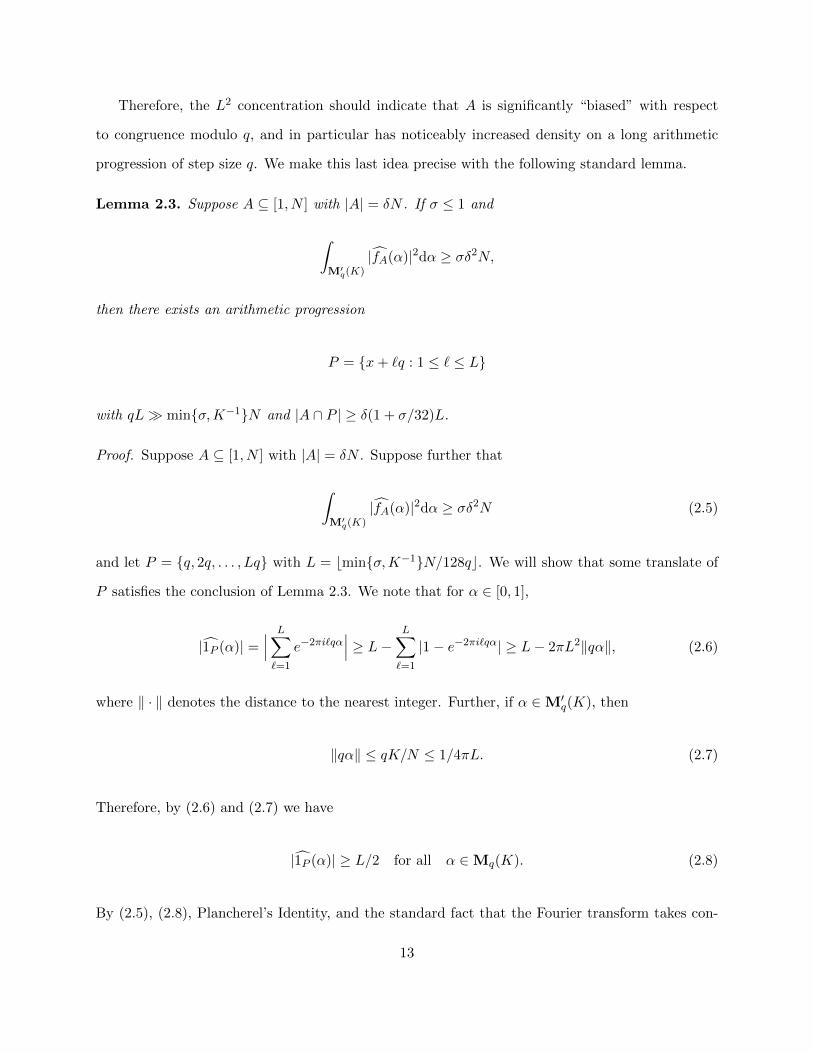
Therefore, the L2 concentration should indicate that A is significantly “biased” with respect
to congruence modulo q, and in particular has noticeably increased density on a long arithmetic
progression of step size q. We make this last idea precise with the following standard lemma.
Lemma 2.3. Suppose A ⊆ [1, N ] with |A| = δN . If σ ≤ 1 and
∫M′q(K)
|fA(α)|2dα ≥ σδ2N,
then there exists an arithmetic progression
P = {x+ `q : 1 ≤ ` ≤ L}
with qL� min{σ,K−1}N and |A ∩ P | ≥ δ(1 + σ/32)L.
Proof. Suppose A ⊆ [1, N ] with |A| = δN . Suppose further that
∫M′q(K)
|fA(α)|2dα ≥ σδ2N (2.5)
and let P = {q, 2q, . . . , Lq} with L = bmin{σ,K−1}N/128qc. We will show that some translate of
P satisfies the conclusion of Lemma 2.3. We note that for α ∈ [0, 1],
|1P (α)| =∣∣∣ L∑`=1
e−2πi`qα∣∣∣ ≥ L− L∑
`=1
|1− e−2πi`qα| ≥ L− 2πL2‖qα‖, (2.6)
where ‖ · ‖ denotes the distance to the nearest integer. Further, if α ∈M′q(K), then
‖qα‖ ≤ qK/N ≤ 1/4πL. (2.7)
Therefore, by (2.6) and (2.7) we have
|1P (α)| ≥ L/2 for all α ∈Mq(K). (2.8)
By (2.5), (2.8), Plancherel’s Identity, and the standard fact that the Fourier transform takes con-
13
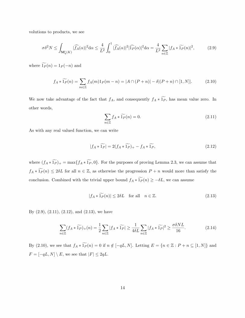
volutions to products, we see
σδ2N ≤∫M′q(K)
|fA(α)|2dα ≤ 4
L2
∫ 1
0|fA(α)|2|1P (α)|2dα =
4
L2
∑n∈Z|fA ∗ 1P (n)|2, (2.9)
where 1P (n) = 1P (−n) and
fA ∗ 1P (n) =∑m∈Z
fA(m)1P (m− n) = |A ∩ (P + n)| − δ|(P + n) ∩ [1, N ]|. (2.10)
We now take advantage of the fact that fA, and consequently fA ∗ 1P , has mean value zero. In
other words, ∑n∈Z
fA ∗ 1P (n) = 0. (2.11)
As with any real valued function, we can write
|fA ∗ 1P | = 2(fA ∗ 1P )+ − fA ∗ 1P , (2.12)
where (fA ∗ 1P )+ = max{fA ∗ 1P , 0}. For the purposes of proving Lemma 2.3, we can assume that
fA ∗ 1P (n) ≤ 2δL for all n ∈ Z, as otherwise the progression P + n would more than satisfy the
conclusion. Combined with the trivial upper bound fA ∗ 1P (n) ≥ −δL, we can assume
|fA ∗ 1P (n)| ≤ 2δL for all n ∈ Z. (2.13)
By (2.9), (2.11), (2.12), and (2.13), we have
∑n∈Z
(fA ∗ 1P )+(n) =1
2
∑n∈Z|fA ∗ 1P | ≥
1
4δL
∑n∈Z|fA ∗ 1P |2 ≥
σδNL
16. (2.14)
By (2.10), we see that fA ∗ 1P (n) = 0 if n /∈ [−qL,N ]. Letting E = {n ∈ Z : P + n ⊆ [1, N ]} and
F = [−qL,N ] \ E, we see that |F | ≤ 2qL.
14
Therefore, by (2.13) and (2.14) we have
∑n∈E
(fA ∗ 1P )+(n) ≥ σδNL
16− 4qδL2 ≥ σδNL
32. (2.15)
Noting that |E| ≤ N and fA ∗ 1P (n) = |A ∩ (P + n)| − δL for all n ∈ E, we have that there exists
n ∈ Z with
|A ∩ (P + n)| ≥ δ(1 + σ/32)L,
as required.
15
3 Sarkozy’s Method for Squares
In this chapter we provide a streamlined exposition of the method used by Sarkozy [22] to prove
Theorem A. We establish the following bound, which is noticeably better than the original.
Theorem 3.1. If A ⊆ [1, N ] and n2 /∈ A−A for all n ∈ N, then
|A|N� log logN
logN.
3.1 Main Iteration Lemma: Deducing Theorem 3.1
We deduce Theorem 3.1 using a density increment iteration, which roughly says that a set with no
square differences spawns a new, denser subset of a slightly smaller interval with an inherited lack
of square differences.
Lemma 3.2. Suppose A ⊆ [1, N ] with |A| = δN and δ ≥ N−1/20. If n2 /∈ A − A for all n ∈ N,
then there exists A′ ⊆ [1, N ′] with
N ′ � δ6N, |A′| ≥ (δ + cδ2)N ′, and n2 /∈ A′ −A′ for all n ∈ N.
Proof of Theorem 3.1
Suppose A ⊆ [1, N ] with |A| = δN and n2 /∈ A − A for all n ∈ N. Setting A0 = A, N0 = N , and
δ0 = δ, Lemma 3.2 yields, for each m, a set Am ⊆ [1, Nm] with |Am| = δmNm and n2 /∈ Am − Am
for all n ∈ N satisfying
Nm ≥ cδ6Nm−1 ≥ (cδ6)mN (3.1)
16
and
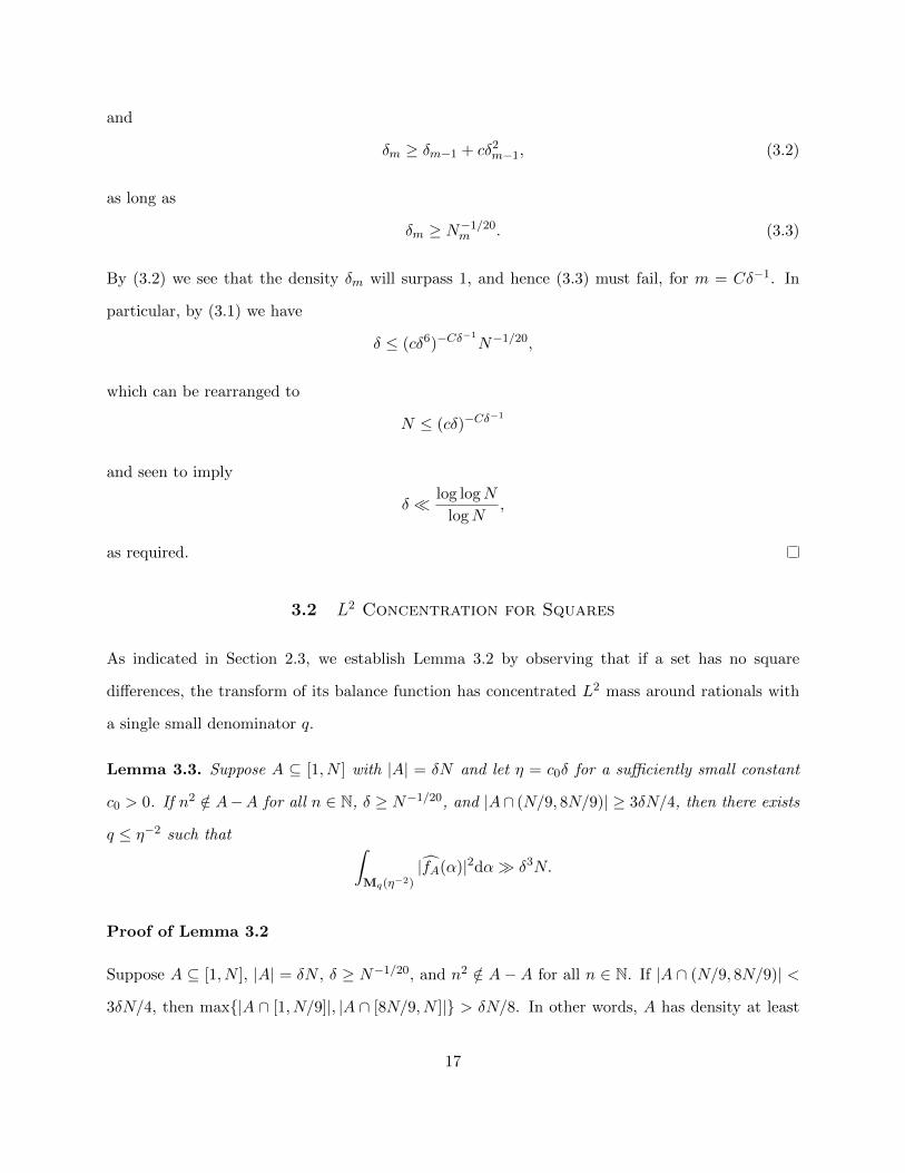
δm ≥ δm−1 + cδ2m−1, (3.2)
as long as
δm ≥ N−1/20m . (3.3)
By (3.2) we see that the density δm will surpass 1, and hence (3.3) must fail, for m = Cδ−1. In
particular, by (3.1) we have
δ ≤ (cδ6)−Cδ−1N−1/20,
which can be rearranged to
N ≤ (cδ)−Cδ−1
and seen to imply
δ � log logN
logN,
as required.
3.2 L2 Concentration for Squares
As indicated in Section 2.3, we establish Lemma 3.2 by observing that if a set has no square
differences, the transform of its balance function has concentrated L2 mass around rationals with
a single small denominator q.
Lemma 3.3. Suppose A ⊆ [1, N ] with |A| = δN and let η = c0δ for a sufficiently small constant
c0 > 0. If n2 /∈ A−A for all n ∈ N, δ ≥ N−1/20, and |A∩ (N/9, 8N/9)| ≥ 3δN/4, then there exists
q ≤ η−2 such that ∫Mq(η−2)
|fA(α)|2dα� δ3N.
Proof of Lemma 3.2
Suppose A ⊆ [1, N ], |A| = δN , δ ≥ N−1/20, and n2 /∈ A− A for all n ∈ N. If |A ∩ (N/9, 8N/9)| <
3δN/4, then max{|A ∩ [1, N/9]|, |A ∩ [8N/9, N ]|} > δN/8. In other words, A has density at least
17
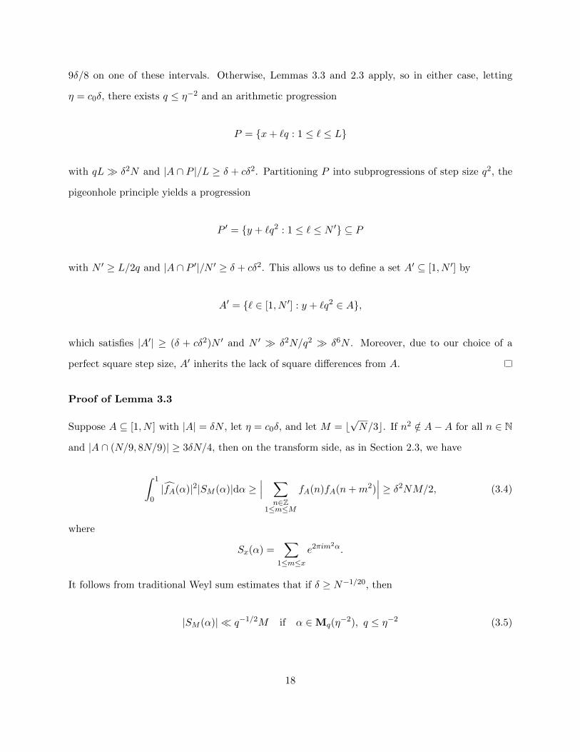
9δ/8 on one of these intervals. Otherwise, Lemmas 3.3 and 2.3 apply, so in either case, letting
η = c0δ, there exists q ≤ η−2 and an arithmetic progression
P = {x+ `q : 1 ≤ ` ≤ L}
with qL � δ2N and |A ∩ P |/L ≥ δ + cδ2. Partitioning P into subprogressions of step size q2, the
pigeonhole principle yields a progression
P ′ = {y + `q2 : 1 ≤ ` ≤ N ′} ⊆ P
with N ′ ≥ L/2q and |A ∩ P ′|/N ′ ≥ δ + cδ2. This allows us to define a set A′ ⊆ [1, N ′] by
A′ = {` ∈ [1, N ′] : y + `q2 ∈ A},
which satisfies |A′| ≥ (δ + cδ2)N ′ and N ′ � δ2N/q2 � δ6N . Moreover, due to our choice of a
perfect square step size, A′ inherits the lack of square differences from A.
Proof of Lemma 3.3
Suppose A ⊆ [1, N ] with |A| = δN , let η = c0δ, and let M = b√N/3c. If n2 /∈ A−A for all n ∈ N
and |A ∩ (N/9, 8N/9)| ≥ 3δN/4, then on the transform side, as in Section 2.3, we have
∫ 1
0|fA(α)|2|SM (α)|dα ≥
∣∣∣ ∑n∈Z
1≤m≤M
fA(n)fA(n+m2)∣∣∣ ≥ δ2NM/2, (3.4)
where
Sx(α) =∑
1≤m≤xe2πim2α.
It follows from traditional Weyl sum estimates that if δ ≥ N−1/20, then
|SM (α)| � q−1/2M if α ∈Mq(η−2), q ≤ η−2 (3.5)
18
and
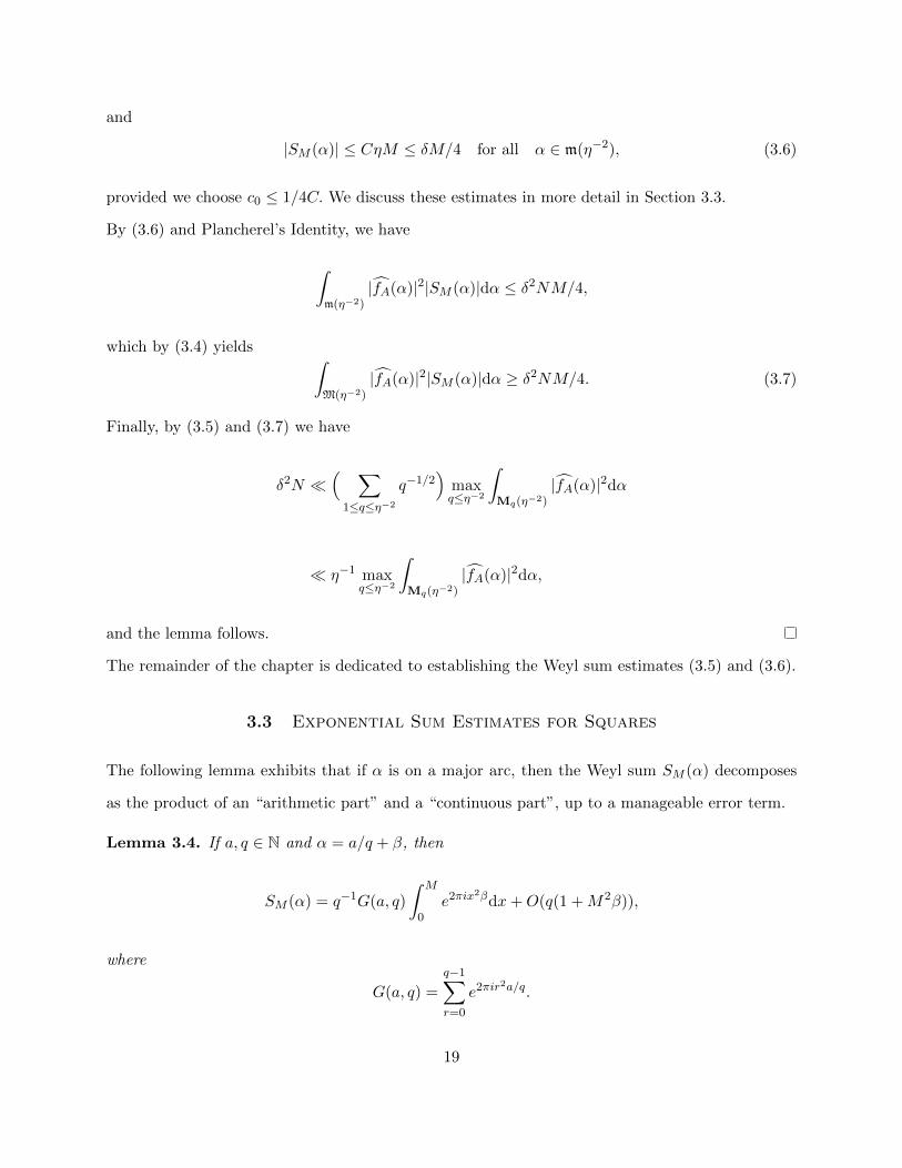
|SM (α)| ≤ CηM ≤ δM/4 for all α ∈ m(η−2), (3.6)
provided we choose c0 ≤ 1/4C. We discuss these estimates in more detail in Section 3.3.
By (3.6) and Plancherel’s Identity, we have
∫m(η−2)
|fA(α)|2|SM (α)|dα ≤ δ2NM/4,
which by (3.4) yields ∫M(η−2)
|fA(α)|2|SM (α)|dα ≥ δ2NM/4. (3.7)
Finally, by (3.5) and (3.7) we have
δ2N �( ∑
1≤q≤η−2
q−1/2)
maxq≤η−2
∫Mq(η−2)
|fA(α)|2dα
� η−1 maxq≤η−2
∫Mq(η−2)
|fA(α)|2dα,
and the lemma follows.
The remainder of the chapter is dedicated to establishing the Weyl sum estimates (3.5) and (3.6).
3.3 Exponential Sum Estimates for Squares
The following lemma exhibits that if α is on a major arc, then the Weyl sum SM (α) decomposes
as the product of an “arithmetic part” and a “continuous part”, up to a manageable error term.
Lemma 3.4. If a, q ∈ N and α = a/q + β, then
SM (α) = q−1G(a, q)
∫ M
0e2πix2βdx+O(q(1 +M2β)),
where
G(a, q) =
q−1∑r=0
e2πir2a/q.
19
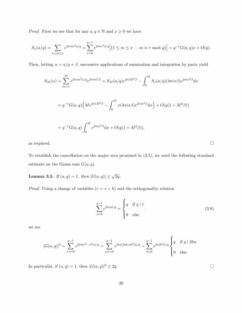
Proof. First we see that for any a, q ∈ N and x ≥ 0 we have
Sx(a/q) =∑
1≤m≤xe2πim2a/q =
q−1∑r=0
e2πir2a/q∣∣∣{1 ≤ m ≤ x : m ≡ r mod q}
∣∣∣ = q−1G(a, q)x+O(q).
Then, letting α = a/q + β, successive applications of summation and integration by parts yield
SM (α) =
M∑m=1
e2πim2a/qe2πim2β = SM (a/q)e2πiM2β −∫ M
0Sx(a/q)(4πixβ)e2πix2βdx
= q−1G(a, q)(Me2πiM2β −
∫ M
0x(4πixβ)e2πix2βdx
)+O(q(1 +M2β))
= q−1G(a, q)
∫ M
0e2πix2βdx+O(q(1 +M2β)),
as required.
To establish the cancellation on the major arcs promised in (3.5), we need the following standard
estimate on the Gauss sum G(a, q).
Lemma 3.5. If (a, q) = 1, then |G(a, q)| ≤√
2q.
Proof. Using a change of variables (r = s+ h) and the orthogonality relation
q−1∑s=0
e2πist/q =
q if q | t
0 else
, (3.8)
we see
|G(a, q)|2 =
q−1∑r,s=0
e2πi(r2−s2)a/q =
q−1∑s,h=0
e2πi(2sh+h2)a/q =
q−1∑h=0
e2πih2a/q
q if q | 2ha
0 else
.
In particular, if (a, q) = 1, then |G(a, q)|2 ≤ 2q.
20
Proof of (3.5)
Since δ �M−1/10, Lemma 3.4 yields
|SM (α)| ≤ q−1|G(a, q)|M +O(M2/5)
provided α ∈Mq(η−2), q ≤ η−2. Applying Lemma 3.5, the estimate follows.
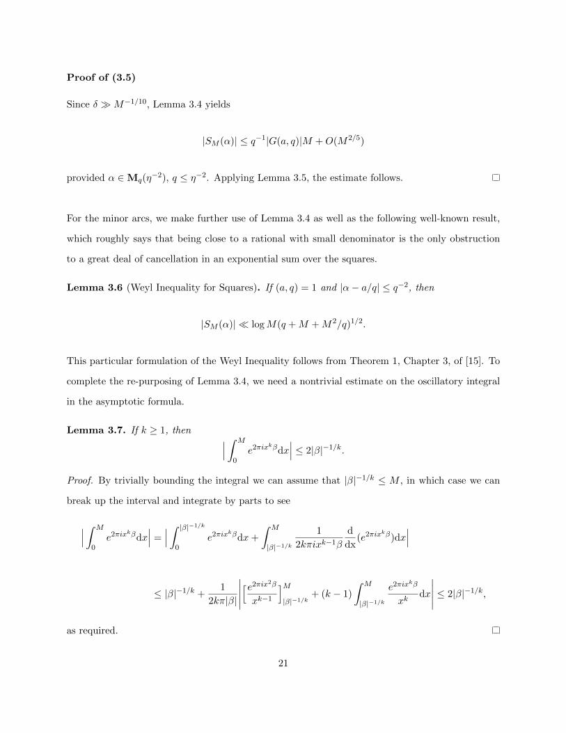
For the minor arcs, we make further use of Lemma 3.4 as well as the following well-known result,
which roughly says that being close to a rational with small denominator is the only obstruction
to a great deal of cancellation in an exponential sum over the squares.
Lemma 3.6 (Weyl Inequality for Squares). If (a, q) = 1 and |α− a/q| ≤ q−2, then
|SM (α)| � logM(q +M +M2/q)1/2.
This particular formulation of the Weyl Inequality follows from Theorem 1, Chapter 3, of [15]. To
complete the re-purposing of Lemma 3.4, we need a nontrivial estimate on the oscillatory integral
in the asymptotic formula.
Lemma 3.7. If k ≥ 1, then ∣∣∣ ∫ M
0e2πixkβdx
∣∣∣ ≤ 2|β|−1/k.
Proof. By trivially bounding the integral we can assume that |β|−1/k ≤ M , in which case we can
break up the interval and integrate by parts to see
∣∣∣ ∫ M
0e2πixkβdx
∣∣∣ =∣∣∣ ∫ |β|−1/k
0e2πixkβdx+
∫ M
|β|−1/k
1
2kπixk−1β
d
dx(e2πixkβ)dx
∣∣∣
≤ |β|−1/k +1
2kπ|β|
∣∣∣∣∣[e2πix2β
xk−1
]M|β|−1/k
+ (k − 1)
∫ M
|β|−1/k
e2πixkβ
xkdx
∣∣∣∣∣ ≤ 2|β|−1/k,
as required.
21
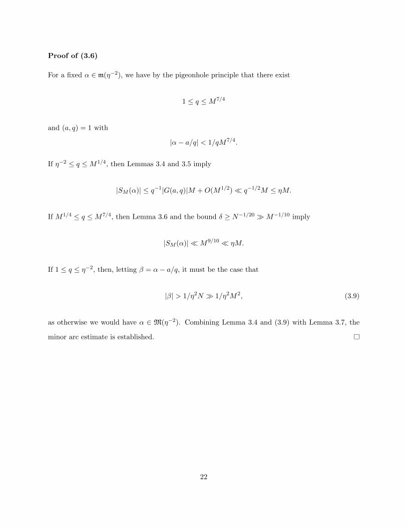
Proof of (3.6)
For a fixed α ∈ m(η−2), we have by the pigeonhole principle that there exist
1 ≤ q ≤M7/4
and (a, q) = 1 with
|α− a/q| < 1/qM7/4.
If η−2 ≤ q ≤M1/4, then Lemmas 3.4 and 3.5 imply
|SM (α)| ≤ q−1|G(a, q)|M +O(M1/2)� q−1/2M ≤ ηM.
If M1/4 ≤ q ≤M7/4, then Lemma 3.6 and the bound δ ≥ N−1/20 �M−1/10 imply
|SM (α)| �M9/10 � ηM.
If 1 ≤ q ≤ η−2, then, letting β = α− a/q, it must be the case that
|β| > 1/η2N � 1/η2M2, (3.9)
as otherwise we would have α ∈ M(η−2). Combining Lemma 3.4 and (3.9) with Lemma 3.7, the
minor arc estimate is established.
22
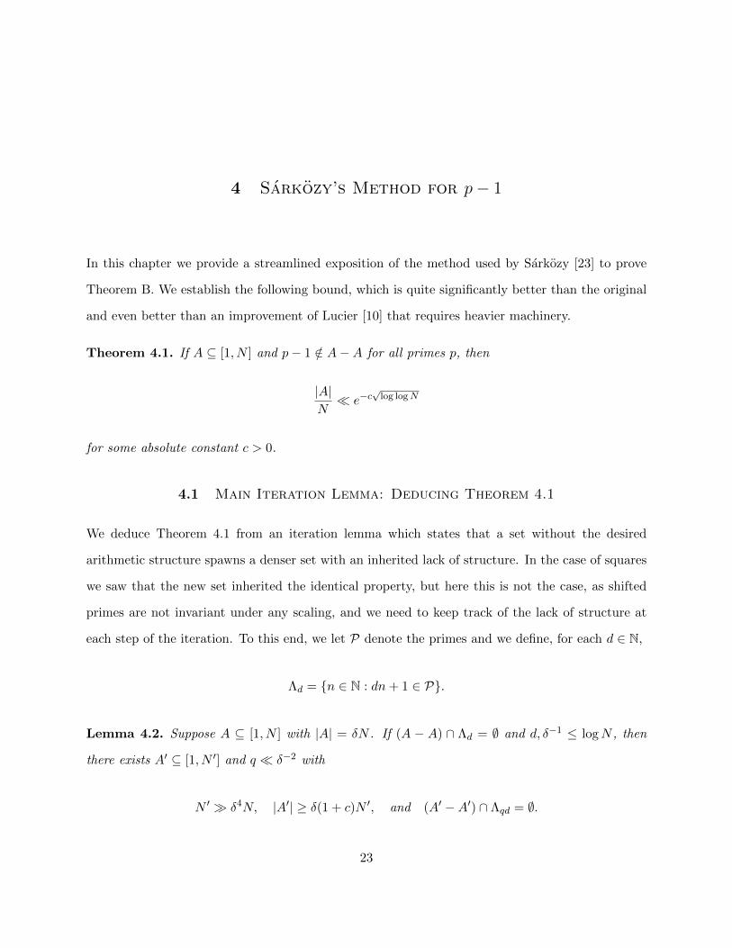
4 Sarkozy’s Method for p− 1
In this chapter we provide a streamlined exposition of the method used by Sarkozy [23] to prove
Theorem B. We establish the following bound, which is quite significantly better than the original
and even better than an improvement of Lucier [10] that requires heavier machinery.
Theorem 4.1. If A ⊆ [1, N ] and p− 1 /∈ A−A for all primes p, then
|A|N� e−c
√log logN
for some absolute constant c > 0.
4.1 Main Iteration Lemma: Deducing Theorem 4.1
We deduce Theorem 4.1 from an iteration lemma which states that a set without the desired
arithmetic structure spawns a denser set with an inherited lack of structure. In the case of squares
we saw that the new set inherited the identical property, but here this is not the case, as shifted
primes are not invariant under any scaling, and we need to keep track of the lack of structure at
each step of the iteration. To this end, we let P denote the primes and we define, for each d ∈ N,
Λd = {n ∈ N : dn+ 1 ∈ P}.
Lemma 4.2. Suppose A ⊆ [1, N ] with |A| = δN . If (A − A) ∩ Λd = ∅ and d, δ−1 ≤ logN , then
there exists A′ ⊆ [1, N ′] and q � δ−2 with
N ′ � δ4N, |A′| ≥ δ(1 + c)N ′, and (A′ −A′) ∩ Λqd = ∅.
23
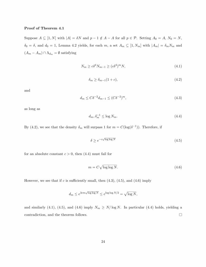
Proof of Theorem 4.1
Suppose A ⊆ [1, N ] with |A| = δN and p − 1 /∈ A − A for all p ∈ P. Setting A0 = A, N0 = N ,
δ0 = δ, and d0 = 1, Lemma 4.2 yields, for each m, a set Am ⊆ [1, Nm] with |Am| = δmNm and
(Am −Am) ∩ Λdm = ∅ satisfying
Nm ≥ cδ4Nm−1 ≥ (cδ4)mN, (4.1)
δm ≥ δm−1(1 + c), (4.2)
and
dm ≤ Cδ−2dm−1 ≤ (Cδ−2)m, (4.3)
as long as
dm, δ−1m ≤ logNm. (4.4)
By (4.2), we see that the density δm will surpass 1 for m = C(log(δ−1)). Therefore, if
δ ≥ e−c√
log logN (4.5)
for an absolute constant c > 0, then (4.4) must fail for
m = C√
log logN. (4.6)
However, we see that if c is sufficiently small, then (4.3), (4.5), and (4.6) imply
dm ≤ e3cm√
log logN ≤ elog logN/2 =√
logN,
and similarly (4.1), (4.5), and (4.6) imply Nm ≥ N/ logN . In particular (4.4) holds, yielding a
contradiction, and the theorem follows.
24
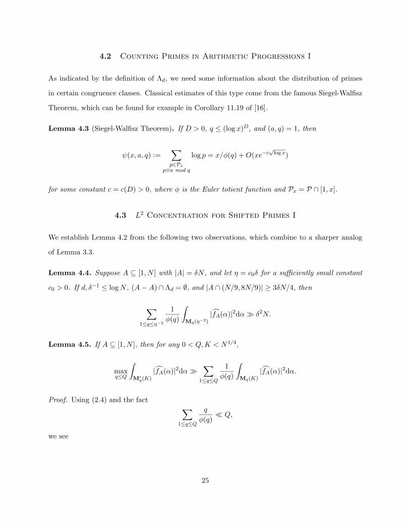
4.2 Counting Primes in Arithmetic Progressions I
As indicated by the definition of Λd, we need some information about the distribution of primes
in certain congruence classes. Classical estimates of this type come from the famous Siegel-Walfisz
Theorem, which can be found for example in Corollary 11.19 of [16].
Lemma 4.3 (Siegel-Walfisz Theorem). If D > 0, q ≤ (log x)D, and (a, q) = 1, then
ψ(x, a, q) :=∑p∈Px
p≡a mod q
log p = x/φ(q) +O(xe−c√
log x)
for some constant c = c(D) > 0, where φ is the Euler totient function and Px = P ∩ [1, x].
4.3 L2 Concentration for Shifted Primes I
We establish Lemma 4.2 from the following two observations, which combine to a sharper analog
of Lemma 3.3.
Lemma 4.4. Suppose A ⊆ [1, N ] with |A| = δN , and let η = c0δ for a sufficiently small constant
c0 > 0. If d, δ−1 ≤ logN , (A−A) ∩ Λd = ∅, and |A ∩ (N/9, 8N/9)| ≥ 3δN/4, then
∑1≤q≤η−2
1
φ(q)
∫Mq(η−2)
|fA(α)|2dα� δ2N.
Lemma 4.5. If A ⊆ [1, N ], then for any 0 < Q,K < N1/4,
maxq≤Q
∫M′q(K)
|fA(α)|2dα�∑
1≤q≤Q
1
φ(q)
∫Mq(K)
|fA(α)|2dα.
Proof. Using (2.4) and the fact ∑1≤q≤Q
q
φ(q)� Q,
we see
25
Qmaxq≤Q
∫M′q(K)
|fA(α)|2dα�∑
1≤q≤Q
q
φ(q)
∫M′q(K)
|fA(α)|2dα
=∑
1≤q≤Q
q
φ(q)
∑r|q
∫Mr(K)
|fA(α)|2dα
=∑
1≤r≤Q
∫Mr(K)
|fA(α)|2dα(r
∑1≤q≤Q/r
q
φ(rq)
)
� Q∑
1≤r≤Q
1
φ(r)
∫Mr(K)
|fA(α)|2dα,
and the lemma follows.
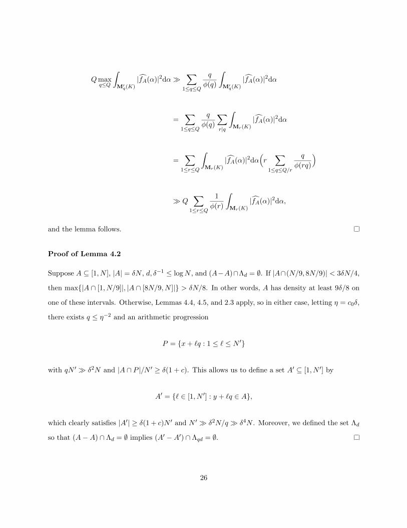
Proof of Lemma 4.2
Suppose A ⊆ [1, N ], |A| = δN , d, δ−1 ≤ logN , and (A−A)∩Λd = ∅. If |A∩(N/9, 8N/9)| < 3δN/4,
then max{|A ∩ [1, N/9]|, |A ∩ [8N/9, N ]|} > δN/8. In other words, A has density at least 9δ/8 on
one of these intervals. Otherwise, Lemmas 4.4, 4.5, and 2.3 apply, so in either case, letting η = c0δ,
there exists q ≤ η−2 and an arithmetic progression
P = {x+ `q : 1 ≤ ` ≤ N ′}
with qN ′ � δ2N and |A ∩ P |/N ′ ≥ δ(1 + c). This allows us to define a set A′ ⊆ [1, N ′] by
A′ = {` ∈ [1, N ′] : y + `q ∈ A},
which clearly satisfies |A′| ≥ δ(1 + c)N ′ and N ′ � δ2N/q � δ4N . Moreover, we defined the set Λd
so that (A−A) ∩ Λd = ∅ implies (A′ −A′) ∩ Λqd = ∅.
26
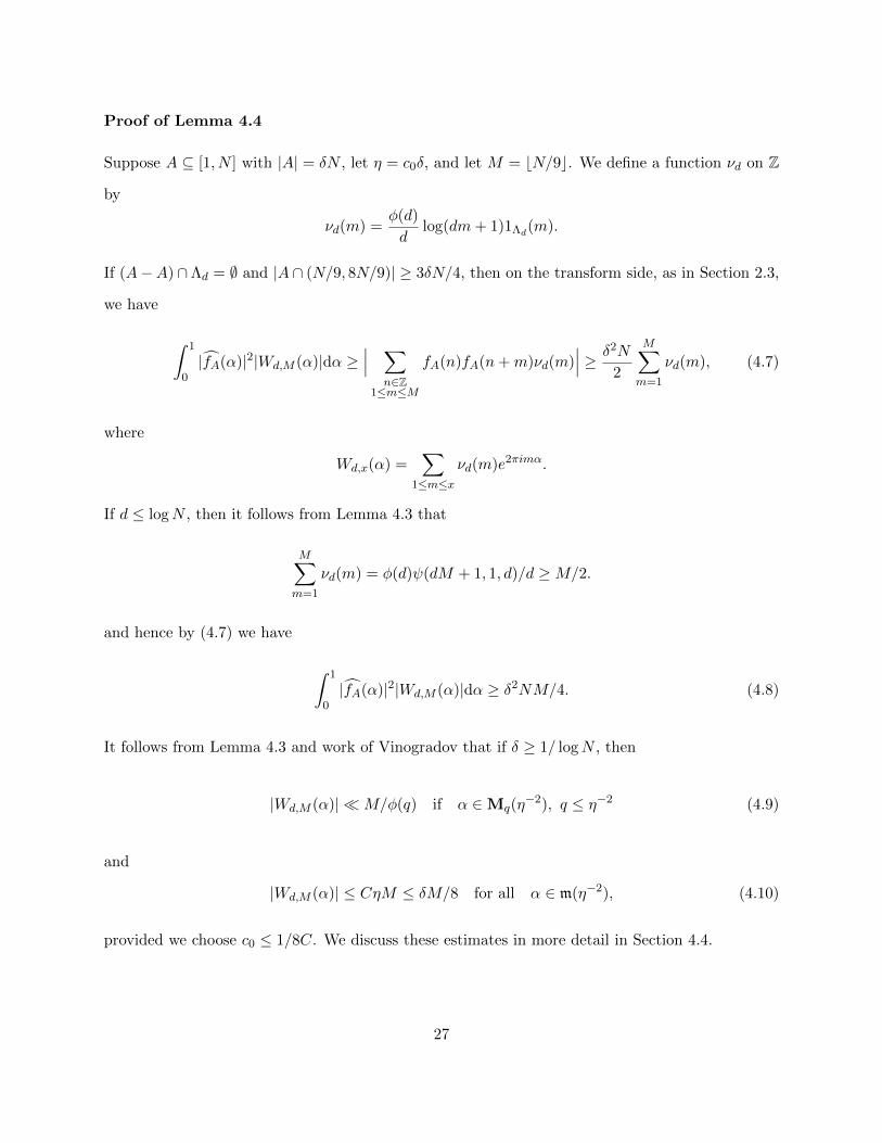
Proof of Lemma 4.4
Suppose A ⊆ [1, N ] with |A| = δN , let η = c0δ, and let M = bN/9c. We define a function νd on Z
by
νd(m) =φ(d)
dlog(dm+ 1)1Λd(m).
If (A−A) ∩Λd = ∅ and |A ∩ (N/9, 8N/9)| ≥ 3δN/4, then on the transform side, as in Section 2.3,
we have
∫ 1
0|fA(α)|2|Wd,M (α)|dα ≥
∣∣∣ ∑n∈Z
1≤m≤M
fA(n)fA(n+m)νd(m)∣∣∣ ≥ δ2N
2
M∑m=1
νd(m), (4.7)
where
Wd,x(α) =∑
1≤m≤xνd(m)e2πimα.
If d ≤ logN , then it follows from Lemma 4.3 that
M∑m=1
νd(m) = φ(d)ψ(dM + 1, 1, d)/d ≥M/2.
and hence by (4.7) we have
∫ 1
0|fA(α)|2|Wd,M (α)|dα ≥ δ2NM/4. (4.8)
It follows from Lemma 4.3 and work of Vinogradov that if δ ≥ 1/ logN , then
|Wd,M (α)| �M/φ(q) if α ∈Mq(η−2), q ≤ η−2 (4.9)
and
|Wd,M (α)| ≤ CηM ≤ δM/8 for all α ∈ m(η−2), (4.10)
provided we choose c0 ≤ 1/8C. We discuss these estimates in more detail in Section 4.4.
27
From (4.8), (4.10), and Plancherel’s Identity, we conclude
∫M(η−2)
|fA(α)|2|Wd,M (α)|dα ≥ δ2NM/8, (4.11)
which by (4.9) implies ∑1≤q≤η−2
1
φ(q)
∫Mq(η−2)
|fA(α)|2dα� δ2N,
as required.
The remainder of the chapter is dedicated to establishing estimates (4.9) and (4.10).
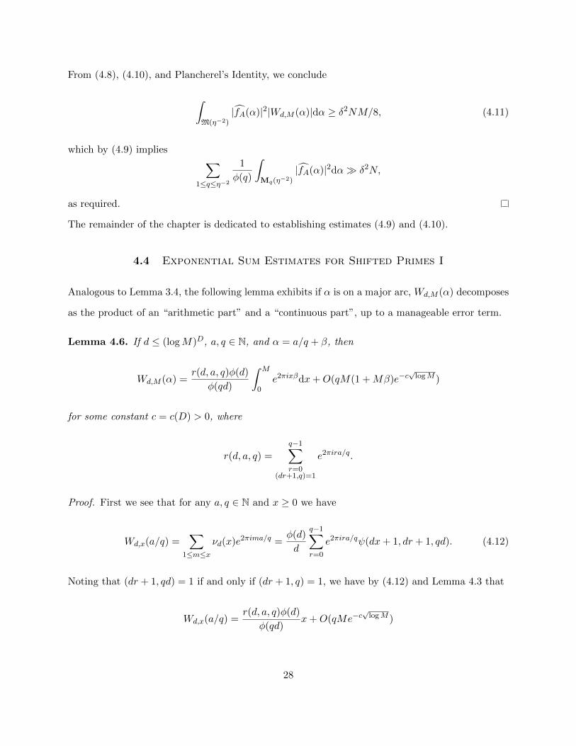
4.4 Exponential Sum Estimates for Shifted Primes I
Analogous to Lemma 3.4, the following lemma exhibits if α is on a major arc, Wd,M (α) decomposes
as the product of an “arithmetic part” and a “continuous part”, up to a manageable error term.
Lemma 4.6. If d ≤ (logM)D, a, q ∈ N, and α = a/q + β, then
Wd,M (α) =r(d, a, q)φ(d)
φ(qd)
∫ M
0e2πixβdx+O(qM(1 +Mβ)e−c
√logM )
for some constant c = c(D) > 0, where
r(d, a, q) =
q−1∑r=0
(dr+1,q)=1
e2πira/q.
Proof. First we see that for any a, q ∈ N and x ≥ 0 we have
Wd,x(a/q) =∑
1≤m≤xνd(x)e2πima/q =
φ(d)
d
q−1∑r=0
e2πira/qψ(dx+ 1, dr + 1, qd). (4.12)
Noting that (dr + 1, qd) = 1 if and only if (dr + 1, q) = 1, we have by (4.12) and Lemma 4.3 that
Wd,x(a/q) =r(d, a, q)φ(d)
φ(qd)x+O(qMe−c
√logM )
28
for all x ≤M . Then, letting α = a/q+ β, successive applications of summation and integration by
parts yield
Wd,M (α) =M∑m=1
νd(m)e2πima/qe2πimβ
= Wd,M (a/q)e2πiMβ −∫ M
0Wd,x(a/q)(2πiβ)e2πixβdx
=r(d, a, q)φ(d)
φ(qd)
(Me2πiMβ −
∫ M
0x(2πiβ)e2πixβdx
)+O(qM(1 +Mβ)e−c
√logM )
=r(d, a, q)φ(d)
φ(qd)
∫ M
0e2πixβdx+O(qM(1 +Mβ)e−c
√logM ),
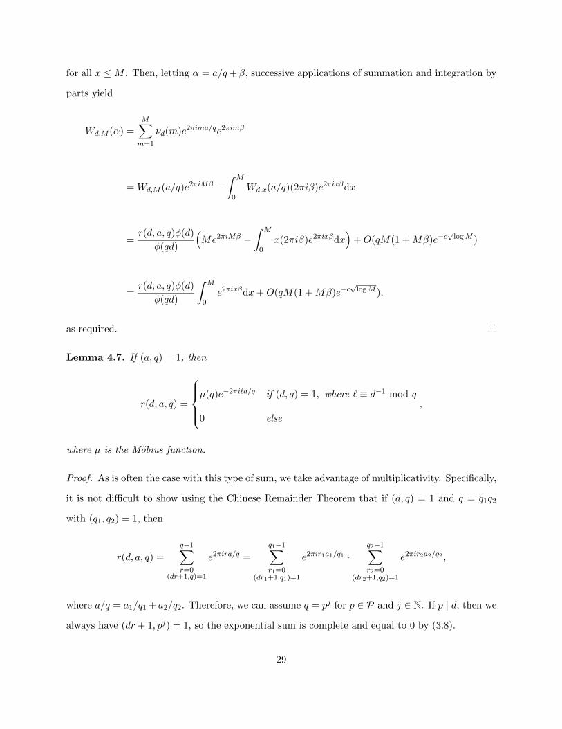
as required.
Lemma 4.7. If (a, q) = 1, then
r(d, a, q) =
µ(q)e−2πi`a/q if (d, q) = 1, where ` ≡ d−1 mod q
0 else
,
where µ is the Mobius function.
Proof. As is often the case with this type of sum, we take advantage of multiplicativity. Specifically,
it is not difficult to show using the Chinese Remainder Theorem that if (a, q) = 1 and q = q1q2
with (q1, q2) = 1, then
r(d, a, q) =
q−1∑r=0
(dr+1,q)=1
e2πira/q =
q1−1∑r1=0
(dr1+1,q1)=1
e2πir1a1/q1 ·q2−1∑r2=0
(dr2+1,q2)=1
e2πir2a2/q2 ,
where a/q = a1/q1 + a2/q2. Therefore, we can assume q = pj for p ∈ P and j ∈ N. If p | d, then we
always have (dr + 1, pj) = 1, so the exponential sum is complete and equal to 0 by (3.8).
29
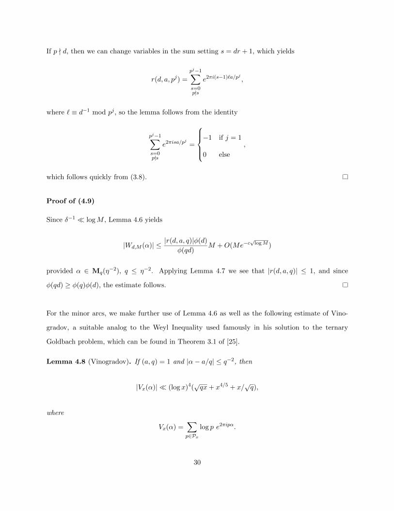
If p - d, then we can change variables in the sum setting s = dr + 1, which yields
r(d, a, pj) =
pj−1∑s=0p-s
e2πi(s−1)`a/pj ,
where ` ≡ d−1 mod pj , so the lemma follows from the identity
pj−1∑s=0p-s
e2πisa/pj =
−1 if j = 1
0 else
,
which follows quickly from (3.8).
Proof of (4.9)
Since δ−1 � logM , Lemma 4.6 yields
|Wd,M (α)| ≤ |r(d, a, q)|φ(d)
φ(qd)M +O(Me−c
√logM )
provided α ∈ Mq(η−2), q ≤ η−2. Applying Lemma 4.7 we see that |r(d, a, q)| ≤ 1, and since
φ(qd) ≥ φ(q)φ(d), the estimate follows.
For the minor arcs, we make further use of Lemma 4.6 as well as the following estimate of Vino-
gradov, a suitable analog to the Weyl Inequality used famously in his solution to the ternary
Goldbach problem, which can be found in Theorem 3.1 of [25].
Lemma 4.8 (Vinogradov). If (a, q) = 1 and |α− a/q| ≤ q−2, then
|Vx(α)| � (log x)4(√qx+ x4/5 + x/
√q),
where
Vx(α) =∑p∈Px
log p e2πipα.
30
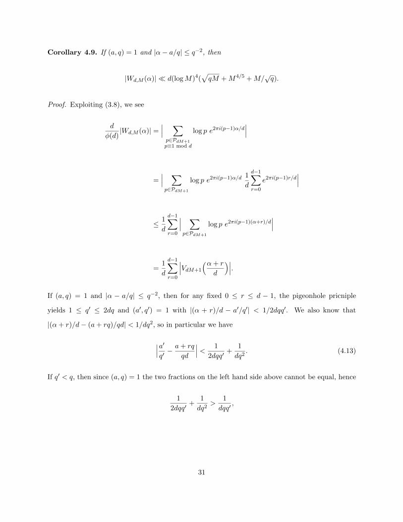
Corollary 4.9. If (a, q) = 1 and |α− a/q| ≤ q−2, then
|Wd,M (α)| � d(logM)4(√qM +M4/5 +M/
√q).
Proof. Exploiting (3.8), we see
d
φ(d)|Wd,M (α)| =
∣∣∣ ∑p∈PdM+1p≡1 mod d
log p e2πi(p−1)α/d∣∣∣
=∣∣∣ ∑p∈PdM+1
log p e2πi(p−1)α/d 1
d
d−1∑r=0
e2πi(p−1)r/d∣∣∣
≤ 1
d
d−1∑r=0
∣∣∣ ∑p∈PdM+1
log p e2πi(p−1)(α+r)/d∣∣∣
=1
d
d−1∑r=0
∣∣∣VdM+1
(α+ r
d
)∣∣∣.If (a, q) = 1 and |α − a/q| ≤ q−2, then for any fixed 0 ≤ r ≤ d − 1, the pigeonhole pricniple
yields 1 ≤ q′ ≤ 2dq and (a′, q′) = 1 with |(α + r)/d − a′/q′| < 1/2dqq′. We also know that
|(α+ r)/d− (a+ rq)/qd| < 1/dq2, so in particular we have
∣∣∣a′q′− a+ rq
qd
∣∣∣ < 1
2dqq′+
1
dq2. (4.13)
If q′ < q, then since (a, q) = 1 the two fractions on the left hand side above cannot be equal, hence
1
2dqq′+
1
dq2>
1
dqq′,
31
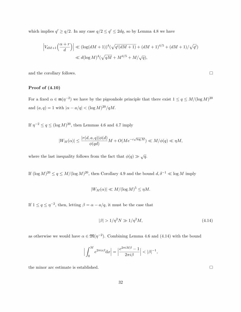
which implies q′ ≥ q/2. In any case q/2 ≤ q′ ≤ 2dq, so by Lemma 4.8 we have
∣∣∣VdM+1
(α+ r
d
)∣∣∣� (log(dM + 1))4(√q′(dM + 1) + (dM + 1)4/5 + (dM + 1)/
√q′)
� d(logM)4(√qM +M4/5 +M/
√q),
and the corollary follows.
Proof of (4.10)
For a fixed α ∈ m(η−2) we have by the pigeonhole principle that there exist 1 ≤ q ≤ M/(logM)20
and (a, q) = 1 with |α− a/q| < (logM)20/qM.
If η−2 ≤ q ≤ (logM)20, then Lemmas 4.6 and 4.7 imply
|WM (α)| ≤ |r(d, a, q)|φ(d)
φ(qd)M +O(Me−c
√logM )�M/φ(q)� ηM,
where the last inequality follows from the fact that φ(q)� √q.
If (logM)20 ≤ q ≤M/(logM)20, then Corollary 4.9 and the bound d, δ−1 � logM imply
|WM (α)| �M/(logM)5 ≤ ηM.
If 1 ≤ q ≤ η−2, then, letting β = α− a/q, it must be the case that
|β| > 1/η2N � 1/η2M, (4.14)
as otherwise we would have α ∈M(η−2). Combining Lemma 4.6 and (4.14) with the bound
∣∣∣ ∫ M
0e2πixβdx
∣∣∣ =∣∣∣e2πiMβ − 1
2πiβ
∣∣∣ < |β|−1,
the minor arc estimate is established.
32
5 Ruzsa-Sanders’ Improvement for p− 1
In this chapter, we provide an exposition of the method used by Ruzsa and Sanders [21] to drastically
improve the bound in Theorem B.
Theorem 5.1 (Ruzsa, Sanders, [21]). If A ⊆ [1, N ] and p− 1 /∈ A−A for all primes p, then
|A|N� e−c(logN)1/4
for an absolute constant c > 0.
5.1 Counting Primes in Arithmetic Progressions II
Ruzsa and Sanders [21] established asymptotics for ψ(x, a, q) for certain moduli q beyond the
limitations of Lemma 4.3 by exploiting a dichotomy based on exceptional zeros, or lack thereof, of
Dirichlet L-functions. In particular, the following result follows from their work.
Lemma 5.2. For any Q,D > 0, there exist q0 ≤ QD and ρ ∈ [1/2, 1) with (1 − ρ)−1 � q0 such
that
ψ(x, a, q) =x
φ(q)− χ(a)xρ
φ(q)ρ+O
(x exp
(− c log x√
log x+D2 logQ
)D2 logQ
), (5.1)
where χ is a Dirichlet character modulo q0, provided q0 | q, (a, q) = 1, and q ≤ (q0Q)D.
Lemma 5.2 is a purpose-built special case of Proposition 4.7 of [21], which in the language of that
paper can be deduced by considering the pair (QD2+D, QD), where q0 is the modulus of the excep-
tional Dirichlet character if the pair is exceptional and q0 = 1 if the pair is unexceptional.
33
It is a calculus exercise to verify that if ε ∈ [0, 1/2] and x ≥ 16, then 1 − x−ε/(1 − ε) ≥ ε, which
implies that the main term in Lemma 5.2 satisfies
<(
(x− χ(a)xρ/ρ)/φ(q))≥ (1− ρ)x/φ(q)� x/q0φ(q). (5.2)
5.2 Main Iteration Lemma: Deducing Theorem 5.1
For the remainder of the argument, we fix a natural number N , and we set Q = ec√
logN for a
sufficiently small constant c > 0. Applying Lemma 5.2 with D = 6, we let q0 ≤ Q6, ρ ∈ [1/2, 1),
and the Dirichlet character χ be as in the conclusion. We see that if c is sufficiently small and
X ≥ N1/3, then
ψ(x, a, q) =x
φ(q)− χ(a)xρ
φ(q)ρ+O(XQ−100) (5.3)
for all x ≤ X, provided q0 | q, (a, q) = 1, and q ≤ (q0Q)6. After passing to a subprogression of step
size q0, we deduce Theorem 5.1 from an iteration lemma analogous to Lemma 4.2.
Lemma 5.3. Suppose A ⊆ [1, L] with |A| = δL and L ≥√N . If q0 | d, (A − A) ∩ Λd = ∅, and
d/q0, δ−1 ≤ Q, then there exists q � δ−2 and A′ ⊆ [1, L′] with
L′ � δ4L, |A′| ≥ δ(1 + c)L′, and (A′ −A′) ∩ Λqd = ∅.
Proof of Theorem 5.1
Suppose A ⊆ [1, N ] with |A| = δN and p − 1 /∈ A − A for all primes p. Partitioning [1, N ], the
pigeonhole principle guarantees the existence of an arithmetic progression
P = {x+ `q0 : 1 ≤ ` ≤ N0} ⊆ [1, N ]
with N0 ≥ N/2q0 and |A ∩ P | ≥ δN0. Defining A0 ⊆ [1, N0] by
A′ = {` ∈ [1, N0] : x+ `q0 ∈ A},
34
we see that |A0| ≥ δN0 and (A− A) ∩ Λq0 = ∅. If δ ≥ Q−1, then Lemma 5.3 yields, for each m, a
set Am ⊆ [1, Nm] with |Am| = δmNm and (Am −Am) ∩ Λdm = ∅ satisfying q0 | d,
Nm ≥ cδ4Nm−1 ≥ (cδ4)mN/q0, (5.4)
δm ≥ δm−1(1 + c), (5.5)
and
dm ≤ Cδ−2dm−1 ≤ (Cδ−2)mq0, (5.6)
as long as
dm/q0 ≤ Q. (5.7)
and
Nm ≥√N. (5.8)
By (4.2), we see that the density δm will surpass 1 for m = C(log(δ−1)). Therefore, if
δ ≥ e−c(logN)1/4 (5.9)
for an absolute constant c > 0, then (5.7) or (5.8) must fail for
m = C(logN)1/4. (5.10)
However, we see that if c is sufficiently small, then (5.6), (5.9), and (5.10) imply
dm/q0 ≤ e3cm(logN)1/4 ≤ ec1√
logN/2 = Q1/2,
and similarly (5.4), (5.9), and (5.10) imply Nm ≥ N/Q20. In particular (5.7) and (5.8) hold, yielding
a contradiction, and the theorem follows.
35
5.3 L2 Concentration for Shifted Primes II
We establish Lemma 5.3 from the following analog of Lemma 4.4.
Lemma 5.4. Suppose A ⊆ [1, L] with |A| = δL and L ≥√N , and let η = c0δ. If q0 | d,
d/q0, δ−1 ≤ Q, (A−A) ∩ Λd = ∅, and |A ∩ (L/9, 8L/9)| ≥ 3δL/4, then
∑1≤q≤η−2
1
φ(q)
∫Mq(η−2)
|fA(α)|2dα� δ2L.
The deduction of Lemma 5.3 from Lemma 5.4 and Lemma 4.5 is completely identical to the de-
duction of Lemma 4.2 from Lemma 4.4 and Lemma 4.5.
Proof of Lemma 5.4
Suppose A ⊆ [1, L] with |A| = δL and (A − A) ∩ Λd = ∅. Let η = c0δ, let M = bL/9c, and let νd
and Wx,d be as in the proof of Lemma 4.4. If |A ∩ (L/9, 8L/9)| ≥ 3δL/4, then just as before we
have
∫ 1
0|fA(α)|2|Wd,M (α)|dα ≥
∣∣∣ ∑n∈Z
1≤m≤M
fA(n)fA(n+m)νd(m)∣∣∣ ≥ δ2L
2
M∑m=1
νd(m) = −δ2LΨ/2,
where Ψ = φ(d)ψ(dM + 1, 1, d)/d. It follows from Lemma 4.7, Lemma 4.9, and (5.3) that if q0 | d
and d/q0, δ−1 ≤ Q, then
|Wd,M (α)| � Ψ/φ(q) if α ∈Mq(η−2), q ≤ η−2 (5.11)
and
|Wd,M (α)| ≤ CηΨ ≤ δΨ/8 for all α ∈ m(η−2). (5.12)
We discuss these estimates in more detail in Section 5.4, and the remainder of the proof is identical
to that of Lemma 4.4.
The remainder of the chapter is dedicated to establishing estimates (5.11) and (5.12).
36
5.4 Exponential Sum Estimates for Shifted Primes II
The following lemma is nearly identical to Lemma 4.6, just applying (5.3) in place of Lemma 4.3.
Lemma 5.5. If q0 | d, d/q0 ≤ Q, a, q ∈ N, q ≤ (q0Q)5, and α = a/q + β, then
Wd,M (α) =r(d, a, q)φ(d)
φ(qd)
∫ M
0(1− (dx)ρ−1)e2πixβdx+O(qM(1 +Mβ)Q−90),
where r(d, a, q) is as in Lemma 4.6.
Proof. Just as in the proof of Lemma 4.6, we see
Wd,x(a/q) =φ(d)
d
q−1∑r=0
e2πira/qψ(dx+ 1, dr + 1, qd) (5.13)
for any x ≥ 0. Noting that (dr + 1, qd) = 1 if and only if (dr + 1, q) = 1, we have by (5.13), (5.3),
and the observation that χ(dr + 1) = χ(1) = 1 because q0 | d, that
Wd,x(a/q) =r(d, a, q)φ(d)
φ(qd)(x− (dx)ρ/ρd) +O(qMQ−90)
for all x ≤M . Observing that
d
dx
(x− (dx)ρ/ρd
)= 1− (dx)ρ−1,
the remainder of the proof is identical to that of Lemma 4.6.
Proof of (5.11)
Since δ−1 ≤ Q, Lemmas 5.5 and 4.7 yield
|Wd,M (α)| ≤ |r(d, a, q)|φ(d)
φ(qd)(M − (dM)ρ/ρd) +O(MQ−80)
≤ Ψ/φ(q) +O(MQ−80),
37
provided α ∈Mq(η−2), q ≤ η−2. By (5.3) and (5.2) we know that
Ψ� (1− ρ)M �M/q0 ≥M/Q6, (5.14)
so the error term is negligible and the estimate follows.
Proof of (5.12)
For a fixed α ∈ m(η−2) we have by the pigeonhole principle that there exist
1 ≤ q ≤M/(q0Q)5
and (a, q) = 1 with
|α− a/q| < (q0Q)5/qM.
If η−2 ≤ q ≤ (q0Q)5, then Lemma 5.5, Lemma 4.7, and (5.14) imply
|WM (α)| ≤ |r(d, a, q)|φ(d)
φ(qd)(M + (dM)ρ/ρd) +O(MQ−10)� Ψ/φ(q)� ηΨ,
where the last inequality follows from the fact that φ(q)� √q.
If (q0Q)5 ≤ q ≤M/(q0Q)5, then Corollary 4.9, (5.14), and the bound d/q0, δ−1 � Q imply
|WM (α)| �M/q0Q� ηΨ.
If 1 ≤ q ≤ η−2, then, letting β = α− a/q, it must be the case that
|β| > 1/η2L� 1/η2M, (5.15)
as otherwise we would have α ∈M(η−2).
38
By Lemma 5.5, (5.14), (5.15), and integration by parts, we have
|WM (α)| ≤∣∣∣ ∫ M
0(1− (dx)ρ−1)e2πixβdx
∣∣∣+O(MQ−50)
≤ |β|−1(1− (dM)ρ−1) +O(MQ−50)
� η2(M − (dM)ρ/ρd+ 2(1− ρ)M)
� ηΨ,
and the minor arc estimate is established.
39
6 Lucier’s Extension to Intersective Polynomials
In this chapter we provide a streamlined exposition of the method used by Lucier [11] to prove
Theorem D. We establish the following bound, which is very slightly better than the original.
Theorem 6.1. Suppose h ∈ Z[x] is an intersective polynomial of degree k ≥ 2 with positive leading
term. If A ⊆ [1, N ] and h(n) /∈ A−A for all n ∈ N with h(n) > 0, then
|A|N�( log logN
logN
)1/(k−1),
where the implied constant depends only on h.
6.1 Auxiliary Polynomials and Related Definitions
For the remainder of the argument, we fix an intersective polynomial h ∈ Z[x] of degree k ≥ 2
with positive leading term, and we set ρ = 2−10k. We apply the same type of density increment
strategy as in the previous chapters, and as in Chapters 4 and 5, we need to keep track of the
inherited lack of arithmetic structure at each step of the iteration. Specifically, if we start with a
set free of differences in the image of h, it spawns denser sets free of differences in the image of new
polynomials. The following definitions describe all of the polynomials that we could potentially
encounter.
Definition 6.2. For each p ∈ P, we fix p-adic integers zp with h(zp) = 0. By reducing and applying
the Chinese Remainder Theorem, the choices of zp determine, for each natural number d, a unique
integer rd ∈ (−d, 0], which consequently satisfies d | h(rd). We define the function λ on N by letting
λ(p) = pm for each p ∈ P, where m is the multiplicity of zp as a root of h, and then extending it
to be completely multiplicative.
40
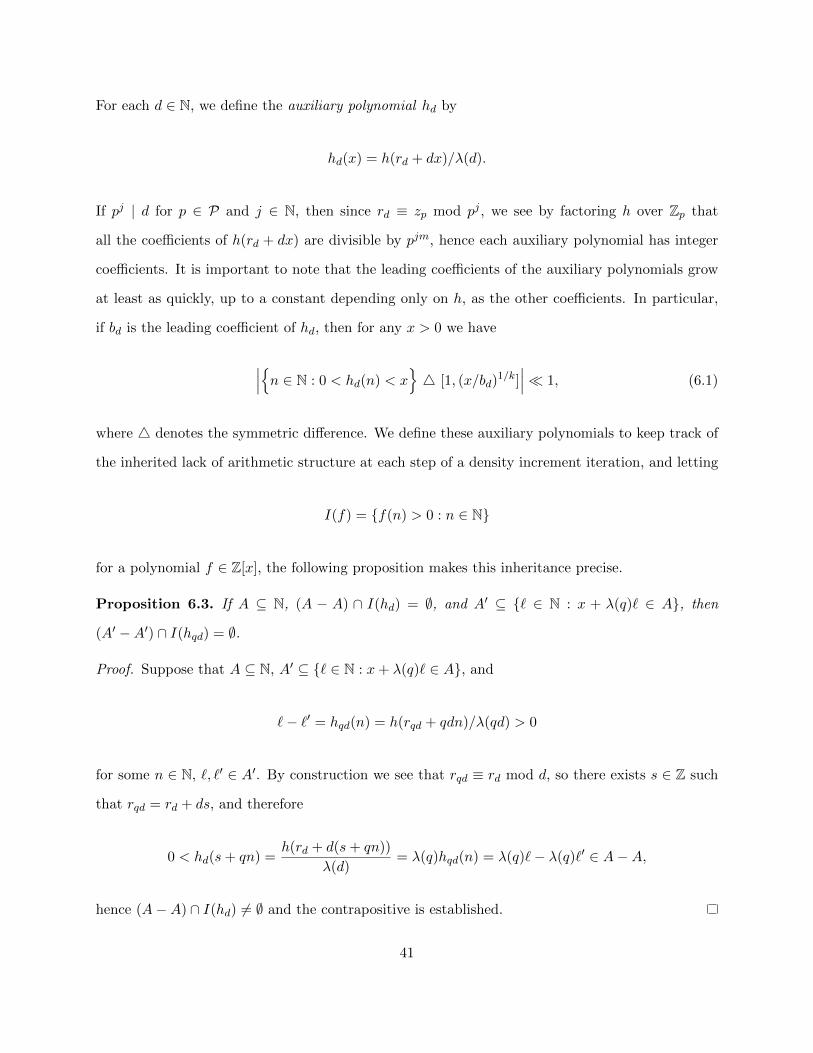
For each d ∈ N, we define the auxiliary polynomial hd by
hd(x) = h(rd + dx)/λ(d).
If pj | d for p ∈ P and j ∈ N, then since rd ≡ zp mod pj , we see by factoring h over Zp that
all the coefficients of h(rd + dx) are divisible by pjm, hence each auxiliary polynomial has integer
coefficients. It is important to note that the leading coefficients of the auxiliary polynomials grow
at least as quickly, up to a constant depending only on h, as the other coefficients. In particular,
if bd is the leading coefficient of hd, then for any x > 0 we have
∣∣∣{n ∈ N : 0 < hd(n) < x}4 [1, (x/bd)
1/k]∣∣∣� 1, (6.1)
where 4 denotes the symmetric difference. We define these auxiliary polynomials to keep track of
the inherited lack of arithmetic structure at each step of a density increment iteration, and letting
I(f) = {f(n) > 0 : n ∈ N}
for a polynomial f ∈ Z[x], the following proposition makes this inheritance precise.
Proposition 6.3. If A ⊆ N, (A − A) ∩ I(hd) = ∅, and A′ ⊆ {` ∈ N : x + λ(q)` ∈ A}, then
(A′ −A′) ∩ I(hqd) = ∅.
Proof. Suppose that A ⊆ N, A′ ⊆ {` ∈ N : x+ λ(q)` ∈ A}, and
`− `′ = hqd(n) = h(rqd + qdn)/λ(qd) > 0
for some n ∈ N, `, `′ ∈ A′. By construction we see that rqd ≡ rd mod d, so there exists s ∈ Z such
that rqd = rd + ds, and therefore
0 < hd(s+ qn) =h(rd + d(s+ qn))
λ(d)= λ(q)hqd(n) = λ(q)`− λ(q)`′ ∈ A−A,
hence (A−A) ∩ I(hd) 6= ∅ and the contrapositive is established.
41
6.2 Main Iteration Lemma: Deducing Theorem 6.1
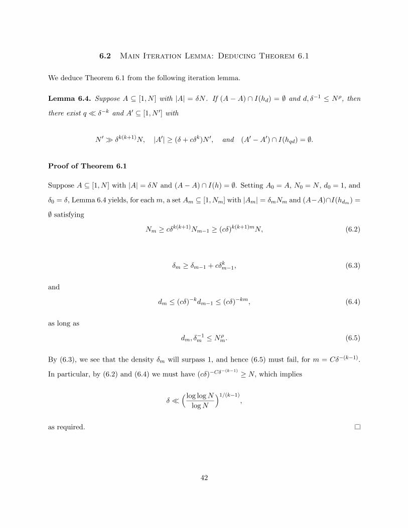
We deduce Theorem 6.1 from the following iteration lemma.
Lemma 6.4. Suppose A ⊆ [1, N ] with |A| = δN . If (A − A) ∩ I(hd) = ∅ and d, δ−1 ≤ Nρ, then
there exist q � δ−k and A′ ⊆ [1, N ′] with
N ′ � δk(k+1)N, |A′| ≥ (δ + cδk)N ′, and (A′ −A′) ∩ I(hqd) = ∅.
Proof of Theorem 6.1
Suppose A ⊆ [1, N ] with |A| = δN and (A−A) ∩ I(h) = ∅. Setting A0 = A, N0 = N , d0 = 1, and
δ0 = δ, Lemma 6.4 yields, for each m, a set Am ⊆ [1, Nm] with |Am| = δmNm and (A−A)∩I(hdm) =
∅ satisfying
Nm ≥ cδk(k+1)Nm−1 ≥ (cδ)k(k+1)mN, (6.2)
δm ≥ δm−1 + cδkm−1, (6.3)
and
dm ≤ (cδ)−kdm−1 ≤ (cδ)−km, (6.4)
as long as
dm, δ−1m ≤ Nρ
m. (6.5)
By (6.3), we see that the density δm will surpass 1, and hence (6.5) must fail, for m = Cδ−(k−1).
In particular, by (6.2) and (6.4) we must have (cδ)−Cδ−(k−1) ≥ N, which implies
δ �( log logN
logN
)1/(k−1),
as required.
42
6.3 L2 Concentration for Auxiliary Polynomials
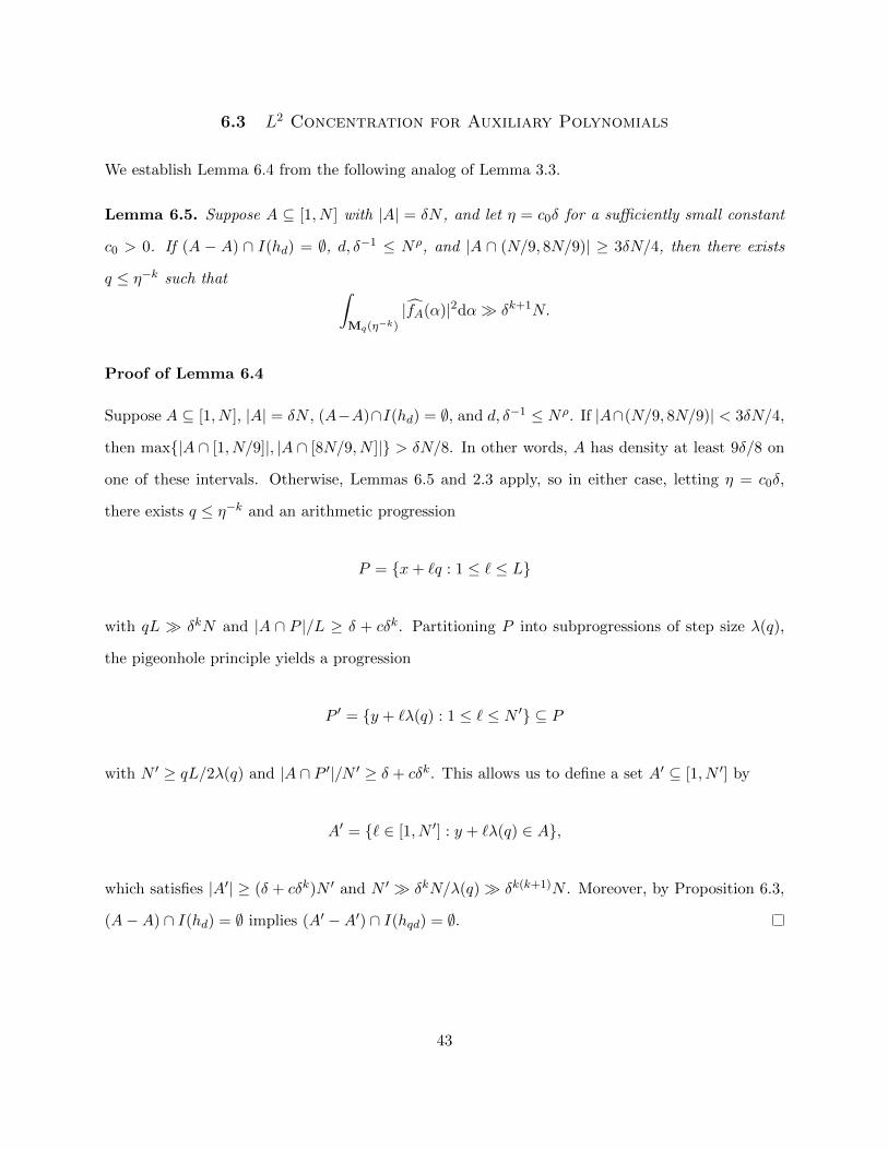
We establish Lemma 6.4 from the following analog of Lemma 3.3.
Lemma 6.5. Suppose A ⊆ [1, N ] with |A| = δN , and let η = c0δ for a sufficiently small constant
c0 > 0. If (A − A) ∩ I(hd) = ∅, d, δ−1 ≤ Nρ, and |A ∩ (N/9, 8N/9)| ≥ 3δN/4, then there exists
q ≤ η−k such that ∫Mq(η−k)
|fA(α)|2dα� δk+1N.
Proof of Lemma 6.4
Suppose A ⊆ [1, N ], |A| = δN , (A−A)∩I(hd) = ∅, and d, δ−1 ≤ Nρ. If |A∩(N/9, 8N/9)| < 3δN/4,
then max{|A ∩ [1, N/9]|, |A ∩ [8N/9, N ]|} > δN/8. In other words, A has density at least 9δ/8 on
one of these intervals. Otherwise, Lemmas 6.5 and 2.3 apply, so in either case, letting η = c0δ,
there exists q ≤ η−k and an arithmetic progression
P = {x+ `q : 1 ≤ ` ≤ L}
with qL � δkN and |A ∩ P |/L ≥ δ + cδk. Partitioning P into subprogressions of step size λ(q),
the pigeonhole principle yields a progression
P ′ = {y + `λ(q) : 1 ≤ ` ≤ N ′} ⊆ P
with N ′ ≥ qL/2λ(q) and |A ∩ P ′|/N ′ ≥ δ + cδk. This allows us to define a set A′ ⊆ [1, N ′] by
A′ = {` ∈ [1, N ′] : y + `λ(q) ∈ A},
which satisfies |A′| ≥ (δ + cδk)N ′ and N ′ � δkN/λ(q)� δk(k+1)N . Moreover, by Proposition 6.3,
(A−A) ∩ I(hd) = ∅ implies (A′ −A′) ∩ I(hqd) = ∅.
43
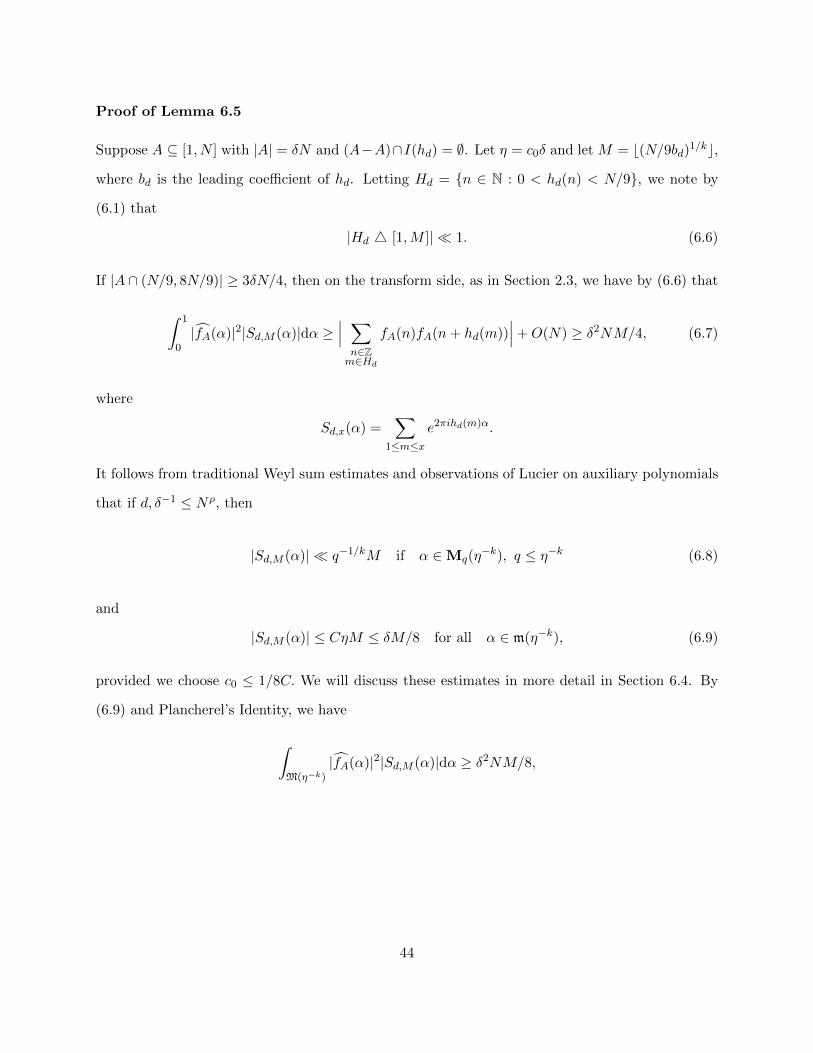
Proof of Lemma 6.5
Suppose A ⊆ [1, N ] with |A| = δN and (A−A)∩I(hd) = ∅. Let η = c0δ and let M = b(N/9bd)1/kc,
where bd is the leading coefficient of hd. Letting Hd = {n ∈ N : 0 < hd(n) < N/9}, we note by
(6.1) that
|Hd 4 [1,M ]| � 1. (6.6)
If |A ∩ (N/9, 8N/9)| ≥ 3δN/4, then on the transform side, as in Section 2.3, we have by (6.6) that
∫ 1
0|fA(α)|2|Sd,M (α)|dα ≥
∣∣∣ ∑n∈Zm∈Hd
fA(n)fA(n+ hd(m))∣∣∣+O(N) ≥ δ2NM/4, (6.7)
where
Sd,x(α) =∑
1≤m≤xe2πihd(m)α.
It follows from traditional Weyl sum estimates and observations of Lucier on auxiliary polynomials
that if d, δ−1 ≤ Nρ, then
|Sd,M (α)| � q−1/kM if α ∈Mq(η−k), q ≤ η−k (6.8)
and
|Sd,M (α)| ≤ CηM ≤ δM/8 for all α ∈ m(η−k), (6.9)
provided we choose c0 ≤ 1/8C. We will discuss these estimates in more detail in Section 6.4. By
(6.9) and Plancherel’s Identity, we have
∫M(η−k)
|fA(α)|2|Sd,M (α)|dα ≥ δ2NM/8,
44
which by (6.7) and (6.8) implies
δ2N �( ∑
1≤q≤η−kq−1/k
)maxq≤η−k
∫Mq(η−k)
|fA(α)|2dα
� η−(k−1) maxq≤η−k
∫Mq(η−k)
|fA(α)|2dα,
and the lemma follows.
The remainder of the chapter is dedicated to establishing estimates (6.8) and (6.9).
6.4 Exponential Sum Estimates over Polynomials
The following lemma generalizes Lemma 3.4 to arbitrary polynomials.
Lemma 6.6. Suppose f(x) = a0 + a1x+ · · ·+ akxk ∈ Z[x] and let J = |a0|+ · · ·+ |ak|. If a, q ∈ N
and α = a/q + β, then
M∑m=1
e2πif(m)α = q−1Gf (a, q)
∫ M
0e2πif(x)βdx+O(q(1 + JMkβ)),
where
Gf (a, q) =
q−1∑r=0
e2πih(r)a/q.
Proof. We begin by noting that for any a, q ∈ N and x ≥ 0,
∑1≤m≤x
e2πif(m)a/q =
q−1∑r=0
∑1≤m≤x
m≡r mod q
e2πif(r)a/q = q−1Gf (a, q)x+O(q), (6.10)
since #{1 ≤ m ≤ x : m ≡ r mod q} = x/q +O(1).
45
Using (6.10) and successive applications of summation and integration by parts, we have that if
α = a/q + β, then
M∑m=1
e2πif(m)α = q−1Gf (a, q)(Me2πif(M)β −
∫ M
0x(2πiβf ′(x))e2πif(x)βdx
)+O(q(1 + JMkβ))
= q−1Gf (a, q)
∫ M
0e2πif(x)βdx+O(q(1 + JMkβ)),
as required.
To establish the cancellation on the major arcs promised in (6.8), we need the following general-
ization of Lemma 3.5, obtained independently by Chen [3] and Nechaev [17].
Lemma 6.7. If f(x) = a0 + a1x+ · · ·+ akxk ∈ Z[x] and (a, q) = 1, then
|Gf (a, q)| � gcd(cont(f), q)1/kq1−1/k,
where
cont(f) = gcd(a1, . . . , ak).
The conclusion of Lemma 6.7 indicates that we could lose control of the sumG(a, q) if the coefficients
of the auxiliary polynomials hd share larger and larger common factors. The following observation
of Lucier ensures that this does not occur.
Lemma 6.8 (Lemma 28, [11]). For every d ∈ N,
cont(hd) ≤ |∆(h)|(k−1)/2cont(h),
where ∆(h) = a2k−2∏i 6=j(αi − αj)eiej if h factors over the complex numbers as
h(x) = a(x− α1)e1 . . . (x− αr)er
with all the αi’s distinct.
46
While the statement of Lemma 6.8 is pleasingly precise, we only use that cont(hd) is uniformly
bounded in terms of the original polynomial h.
Proof of (6.8)
Since
d, δ−1 � Nρ �M2kρ, (6.11)
and all of the coefficients of hd are bounded by a constant times dk−1, Lemma 3.4 yields
|SM (α)| ≤ q−1|Ghd(a, q)|M +O(M6k2ρ)
provided α ∈Mq(η−k), q ≤ η−k. Applying Lemmas 6.7 and 6.8, the estimate follows.
For the minor arcs we now require the full Weyl inequality, which says that when taking an expo-
nential sum over a polynomial, the only obstruction to cancellation is if the leading coefficient is
close to a rational with small denominator.
Lemma 6.9 (Weyl Inequality). If α1, . . . , αk ∈ R, t ≥ 1, (a, q) = 1 and |αk − a/q| ≤ t/q2, then
∣∣∣ M∑m=1
e2πi(α1m+···+αkmk)∣∣∣�M1+ε(t/q + 1/M + t/Mk−1 + q/Mk)21−k
for any ε > 0, where the implied constant depends only on k and ε.
This result is completely standard, and although most treatments, such as Lemma 2.4 of [25], re-
strict to the case of t = 1, this version follows from a trivial modification of the proof.
Corollary 6.10. Suppose f(x) = a0+a1x+· · ·+akxk with ak ∈ N. If (a, q) = 1 and |α−a/q| ≤ q−2,
then ∣∣∣ M∑m=1
e2πif(m)α∣∣∣�M1+ε(ak/q + 1/M + ak/M
k−1 + q/Mk)21−k
for any ε > 0, where the implied constant depends only on k and ε.
47
Proof. Suppose f(x) = a0 + a1x+ · · ·+ akxk with ak ∈ N, (a, q) = 1, and |α− a/q| ≤ q−2. Letting
D = gcd(ak, q), we see that ∣∣∣akα− aka/D
q/D
∣∣∣ ≤ ak/D
(q/D)2,
so by Lemma 6.9 we have
∣∣∣ M∑m=1
e2πif(m)α∣∣∣�M1+ε
(ak/Dq/D
+1
M+ak/D
Mk+1+q/D
Mk
)21−k
,
and the corollary follows.
Proof of (6.9)
For a fixed α ∈ m(η−k), we have by the pigeonhole principle that there exist
1 ≤ q ≤Mk−1/4
and (a, q) = 1 with
|α− a/q| < 1/qMk−1/4.
If η−k ≤ q ≤M1/4, then Lemmas 6.6, 6.7, and 6.8 combine with (6.11) to imply
|SM (α)| ≤ q−1|Ghd(a, q)|M +O(M2/3)� q−1/kM ≤ ηM.
If M1/4 ≤ q ≤Mk−1/4, then Corollary 6.10 and (6.11) imply
|SM (α)| �M1−2−2k ≤M1−2kρ ≤ ηM.
If 1 ≤ q ≤ η−k, then, letting β = α− a/q, it must be the case that
|β| > 1/ηkN � 1/ηkbdMk, (6.12)
where again bd is the leading coefficient of hd, as otherwise we would have α ∈M(η−k).
48
By Lemma 3.7 we have ∣∣∣ ∫ M
0e2πibdx
kβ∣∣∣� |bdβ|−1/k. (6.13)
Combining Lemma 6.6 and (6.12) with (6.13) and the fact that
∣∣∣ ∫ M
0e2πibdx
kβ − e2πihd(x)βdx∣∣∣� dkMkβ ≤M1/2, (6.14)
the minor arc estimate is established.
49
7 P-intersective Polynomials
In this chapter we establish one of our main new results which improves Theorem E in two ways,
expanding the class of polynomials and improving the bound from triple to single logarithmic.
Theorem 7.1. Suppose h ∈ Z[x] is a P-intersective polynomial of degree k ≥ 2 with positive leading
term. If A ⊆ [1, N ] and h(p) /∈ A−A for all p ∈ P with h(p) > 0, then
|A|N� (logN)−µ (7.1)
for any µ < 1/(2k − 2), where the implied constant depends only on h and µ.
7.1 Main Iteration Lemma: Deducing Theorem 7.1
For the remainder of the argument, we fix a P-intersective polynomial h of degree k ≥ 2 with
positive leading term, and we set K = 210k. We also fix an arbitrary ε > 0, we set γ = k + ε,
and we prove Theorem 7.1 with µ = 1/2(γ − 1) + ε. For each p ∈ P we fix a p-adic integer
zp such that h(zp) = 0 and zp 6≡ 0 mod p. By reducing and applying the Chinese Remainder
Theorem, the choices of zp determine, for each natural number d, a unique integer rd ∈ (−d, 0],
which consequently satisfies d | h(rd) and (rd, d) = 1. We let the function λ and the auxiliary
polynomials hd be as in Definition 6.2, we let
Λd = {n ∈ N : rd + dn ∈ P},
and we let
Vd(h) = {hd(n) > 0 : n ∈ Λd}.
50
The following proposition, analogous to Proposition 6.3, shows that the definition of Vd(h) is
appropriate for keeping track of the inherited lack of arithmetic structure in our density increment
iteration.
Proposition 7.2. If A ⊆ N, (A − A) ∩ Vd(h) = ∅, and A′ ⊆ {` ∈ N : x + λ(q)` ∈ A}, then
(A′ −A′) ∩ Vqd(h) = ∅.
Proof. The proof is identical to that of Proposition 6.3, with the added observation that if n ∈ Λqd
and rqd = rd + ds, then s+ qn ∈ Λd.
We also fix a natural number N , and we set Q = ec√
logN for a sufficiently small constant c > 0.
Applying Lemma 5.2 with D = 10K, we let q0 ≤ Q10K , ρ ∈ [1/2, 1), and the Dirichlet character χ
be as in the conclusion. We see that if c is sufficiently small and X ≥ N1/10k, then
ψ(x, a, q) =x
φ(q)− χ(a)xρ
φ(q)ρ+O(XQ−1000K2
) (7.2)
for all x ≤ X, provided q0 | q, (a, q) = 1, and q ≤ (q0Q)10K .
Lemma 7.3. Suppose A ⊆ [1, L] with |A| = δL and L ≥√N . If q0 | d, (A− A) ∩ Vd(h) = ∅, and
d/q0, δ−1 ≤ Q, then there exists q � δ−γ and A′ ⊆ [1, L′] with
L′ � δγ(k+1)L, |A′| ≥ (δ + cδγ)L′, and (A′ −A′) ∩ Vqd(h) = ∅.
Proof of Theorem 7.1
Suppose A ⊆ [1, N ] with |A| = δN and h(p) /∈ A − A for all p ∈ P with h(p) > 0, that is to say
(A − A) ∩ V1(h) = ∅. Partitioning [1, N ], the pigeonhole principle guarantees the existence of an
arithmetic progression
P = {x+ `λ(q0) : 1 ≤ ` ≤ N0} ⊆ [1, N ]
with N0 ≥ N/2λ(q0) and |A ∩ P | ≥ δN0. Defining A0 ⊆ [1, N0] by
A′ = {` ∈ [1, N0] : x+ `λ(q0) ∈ A},
51
we see that |A0| ≥ δN0 and (A−A) ∩ Vq0(h) = ∅. If δ ≥ Q−1, then Lemma 7.3 yields, for each m,
a set Am ⊆ [1, Nm] with |Am| = δmNm and (A−A) ∩ Vdm(h) = ∅ satisfying q0 | d,
Nm ≥ cδγ(k+1)Nm−1 ≥ (cδ)γ(k+1)mN/qk0 , (7.3)
δm ≥ δm−1 + cδγm−1, (7.4)
and
dm ≤ (cδ)−γdm−1 ≤ (cδ)−γmq0, (7.5)
as long as
dm/q0, δ−1m ≤ Q (7.6)
and
Nm ≥√N (7.7)
By (7.4), we see that the density δm will surpass 1, and hence (7.6) must fail, for m = Cδ−(γ−1).
Therefore, if
δ ≥ (logN)−1/2(γ−1)+ε, (7.8)
then (7.6) or (7.7) must fail for
m = C(logN)1/2−ε. (7.9)
However, we see that (7.5), (7.8), and (7.9) imply
dm/q0 ≤ e(logN)1/2−ε/2 ≤ Q,
and similarly (7.3), (7.8), and (7.9) imply Nm ≥ N/QC . In particular (7.6) and (7.7) hold, yielding
a contradiction, and the theorem follows.
52
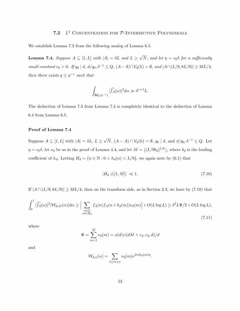
7.2 L2 Concentration for P-Intersective Polynomials
We establish Lemma 7.3 from the following analog of Lemma 6.5.
Lemma 7.4. Suppose A ⊆ [1, L] with |A| = δL and L ≥√N , and let η = c0δ for a sufficiently
small constant c0 > 0. If q0 | d, d/q0, δ−1 ≤ Q, (A−A)∩Vd(h) = ∅, and |A∩(L/9, 8L/9)| ≥ 3δL/4,
then there exists q ≤ η−γ such that
∫Mq(η−γ)
|fA(α)|2dα� δγ+1L.
The deduction of Lemma 7.3 from Lemma 7.4 is completely identical to the deduction of Lemma
6.4 from Lemma 6.5.
Proof of Lemma 7.4
Suppose A ⊆ [1, L] with |A| = δL, L ≥√N , (A − A) ∩ Vd(h) = ∅, q0 | d, and d/q0, δ
−1 ≤ Q. Let
η = c0δ, let νd be as in the proof of Lemma 4.4, and let M = b(L/9bd)1/kc, where bd is the leading
coefficient of hd. Letting Hd = {n ∈ N : 0 < hd(n) < L/9}, we again note by (6.1) that
|Hd 4[1,M ]| � 1. (7.10)
If |A ∩ (L/9, 8L/9)| ≥ 3δL/4, then on the transform side, as in Section 2.3, we have by (7.10) that
∫ 1
0|fA(α)|2|Wd,M (α)|dα ≥
∣∣∣ ∑n∈Zm∈Hd
fA(n)fA(n+hd(m))νd(m)∣∣∣+O(L logL) ≥ δ2LΨ/2 +O(L logL),
(7.11)
where
Ψ =M∑m=1
νd(m) = φ(d)ψ(dM + rd, rd, d)/d
and
Wd,x(α) =∑
1≤m≤xνd(m)e2πihd(m)α.
53
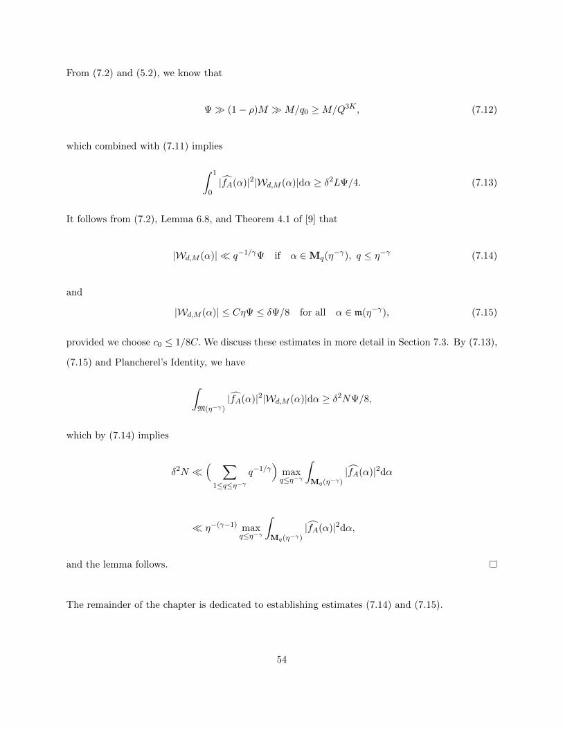
From (7.2) and (5.2), we know that
Ψ� (1− ρ)M �M/q0 ≥M/Q3K , (7.12)
which combined with (7.11) implies
∫ 1
0|fA(α)|2|Wd,M (α)|dα ≥ δ2LΨ/4. (7.13)
It follows from (7.2), Lemma 6.8, and Theorem 4.1 of [9] that
|Wd,M (α)| � q−1/γΨ if α ∈Mq(η−γ), q ≤ η−γ (7.14)
and
|Wd,M (α)| ≤ CηΨ ≤ δΨ/8 for all α ∈ m(η−γ), (7.15)
provided we choose c0 ≤ 1/8C. We discuss these estimates in more detail in Section 7.3. By (7.13),
(7.15) and Plancherel’s Identity, we have
∫M(η−γ)
|fA(α)|2|Wd,M (α)|dα ≥ δ2NΨ/8,
which by (7.14) implies
δ2N �( ∑
1≤q≤η−γq−1/γ
)maxq≤η−γ
∫Mq(η−γ)
|fA(α)|2dα
� η−(γ−1) maxq≤η−γ
∫Mq(η−γ)
|fA(α)|2dα,
and the lemma follows.
The remainder of the chapter is dedicated to establishing estimates (7.14) and (7.15).
54
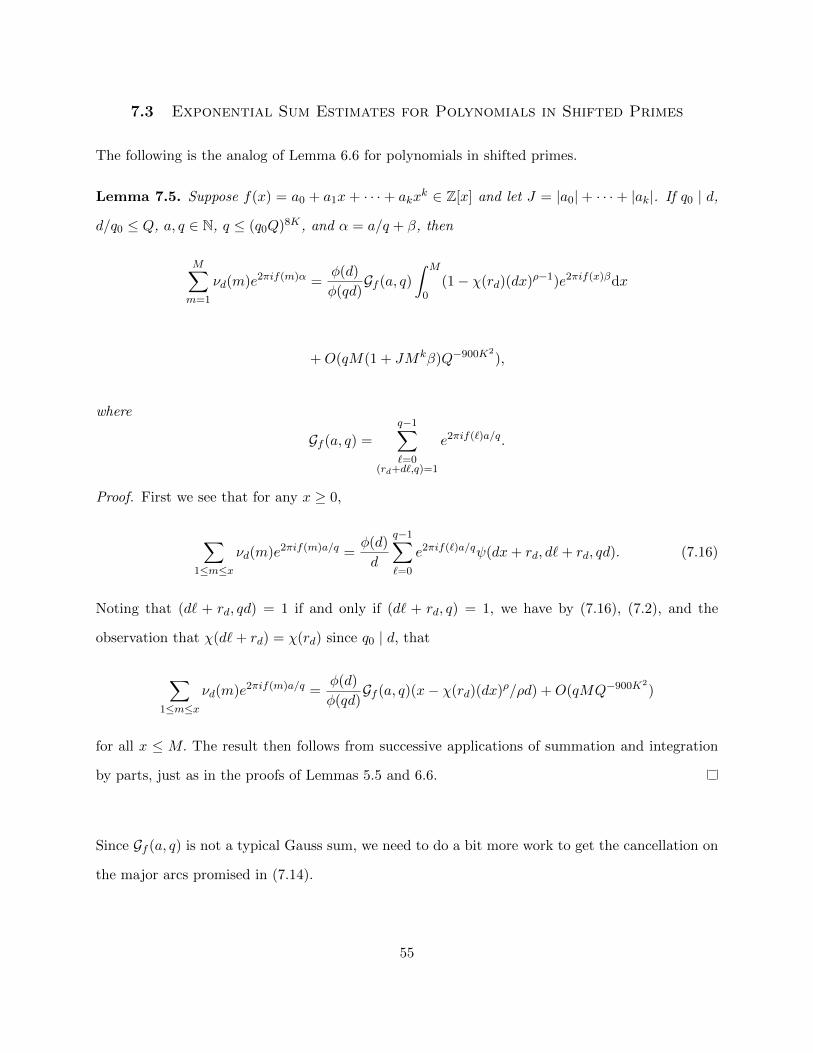
7.3 Exponential Sum Estimates for Polynomials in Shifted Primes
The following is the analog of Lemma 6.6 for polynomials in shifted primes.
Lemma 7.5. Suppose f(x) = a0 + a1x+ · · ·+ akxk ∈ Z[x] and let J = |a0|+ · · ·+ |ak|. If q0 | d,
d/q0 ≤ Q, a, q ∈ N, q ≤ (q0Q)8K , and α = a/q + β, then
M∑m=1
νd(m)e2πif(m)α =φ(d)
φ(qd)Gf (a, q)
∫ M
0(1− χ(rd)(dx)ρ−1)e2πif(x)βdx
+O(qM(1 + JMkβ)Q−900K2),
where
Gf (a, q) =
q−1∑`=0
(rd+d`,q)=1
e2πif(`)a/q.
Proof. First we see that for any x ≥ 0,
∑1≤m≤x
νd(m)e2πif(m)a/q =φ(d)
d
q−1∑`=0
e2πif(`)a/qψ(dx+ rd, d`+ rd, qd). (7.16)
Noting that (d` + rd, qd) = 1 if and only if (d` + rd, q) = 1, we have by (7.16), (7.2), and the
observation that χ(d`+ rd) = χ(rd) since q0 | d, that
∑1≤m≤x
νd(m)e2πif(m)a/q =φ(d)
φ(qd)Gf (a, q)(x− χ(rd)(dx)ρ/ρd) +O(qMQ−900K2
)
for all x ≤ M. The result then follows from successive applications of summation and integration
by parts, just as in the proofs of Lemmas 5.5 and 6.6.
Since Gf (a, q) is not a typical Gauss sum, we need to do a bit more work to get the cancellation on
the major arcs promised in (7.14).
55
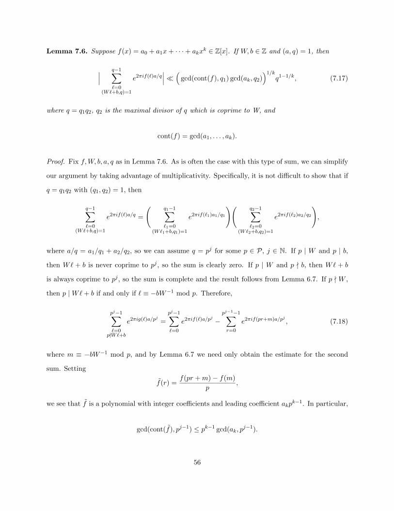
Lemma 7.6. Suppose f(x) = a0 + a1x+ · · ·+ akxk ∈ Z[x]. If W, b ∈ Z and (a, q) = 1, then
∣∣∣ q−1∑`=0
(W`+b,q)=1
e2πif(`)a/q∣∣∣� (
gcd(cont(f), q1) gcd(ak, q2))1/k
q1−1/k, (7.17)
where q = q1q2, q2 is the maximal divisor of q which is coprime to W, and
cont(f) = gcd(a1, . . . , ak).
Proof. Fix f,W, b, a, q as in Lemma 7.6. As is often the case with this type of sum, we can simplify
our argument by taking advantage of multiplicativity. Specifically, it is not difficult to show that if
q = q1q2 with (q1, q2) = 1, then
q−1∑`=0
(W`+b,q)=1
e2πif(`)a/q =
(q1−1∑`1=0
(W`1+b,q1)=1
e2πif(`1)a1/q1
)(q2−1∑`2=0
(W`2+b,q2)=1
e2πif(`2)a2/q2
),
where a/q = a1/q1 + a2/q2, so we can assume q = pj for some p ∈ P, j ∈ N. If p | W and p | b,
then W` + b is never coprime to pj , so the sum is clearly zero. If p | W and p - b, then W` + b
is always coprime to pj , so the sum is complete and the result follows from Lemma 6.7. If p - W ,
then p |W`+ b if and only if ` ≡ −bW−1 mod p. Therefore,
pj−1∑`=0
p-W`+b
e2πig(`)a/pj =
pj−1∑`=0
e2πif(`)a/pj −pj−1−1∑r=0
e2πif(pr+m)a/pj , (7.18)
where m ≡ −bW−1 mod p, and by Lemma 6.7 we need only obtain the estimate for the second
sum. Setting
f(r) =f(pr +m)− f(m)
p,
we see that f is a polynomial with integer coefficients and leading coefficient akpk−1. In particular,
gcd(cont(f), pj−1) ≤ pk−1 gcd(ak, pj−1).
56
Therefore, by Lemma 6.7 we have
∣∣∣ pj−1−1∑r=0
e2πif(pr+m)a/pj∣∣∣ =
∣∣∣ pj−1−1∑r=0
e2πi(f(pr+m)−f(m))a/pj∣∣∣
=∣∣∣ pj−1−1∑
r=0
e2πif(r)a/pj−1∣∣∣
�(pk−1 gcd(ak, p
j−1))1/k
p(j−1)(1−1/k)
≤ gcd(ak, pj)1/kpj(1−1/k),
as required.
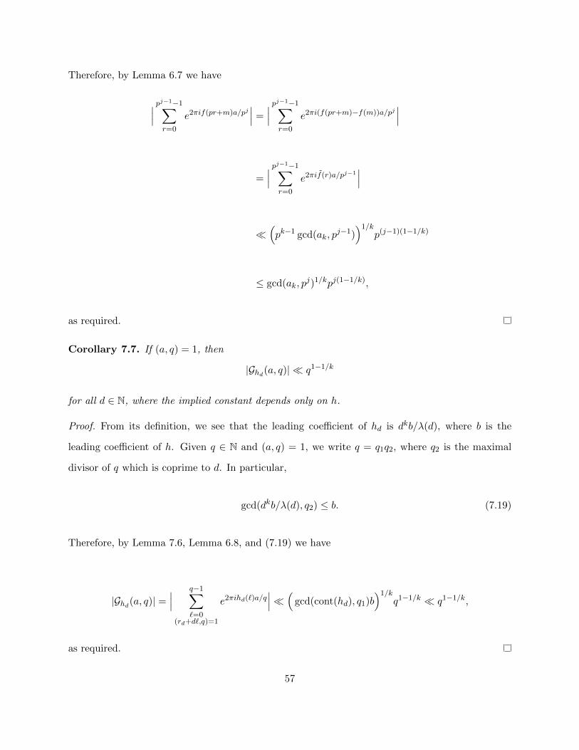
Corollary 7.7. If (a, q) = 1, then
|Ghd(a, q)| � q1−1/k
for all d ∈ N, where the implied constant depends only on h.
Proof. From its definition, we see that the leading coefficient of hd is dkb/λ(d), where b is the
leading coefficient of h. Given q ∈ N and (a, q) = 1, we write q = q1q2, where q2 is the maximal
divisor of q which is coprime to d. In particular,
gcd(dkb/λ(d), q2) ≤ b. (7.19)
Therefore, by Lemma 7.6, Lemma 6.8, and (7.19) we have
|Ghd(a, q)| =∣∣∣ q−1∑
`=0(rd+d`,q)=1
e2πihd(`)a/q∣∣∣� (
gcd(cont(hd), q1)b)1/k
q1−1/k � q1−1/k,
as required.
57
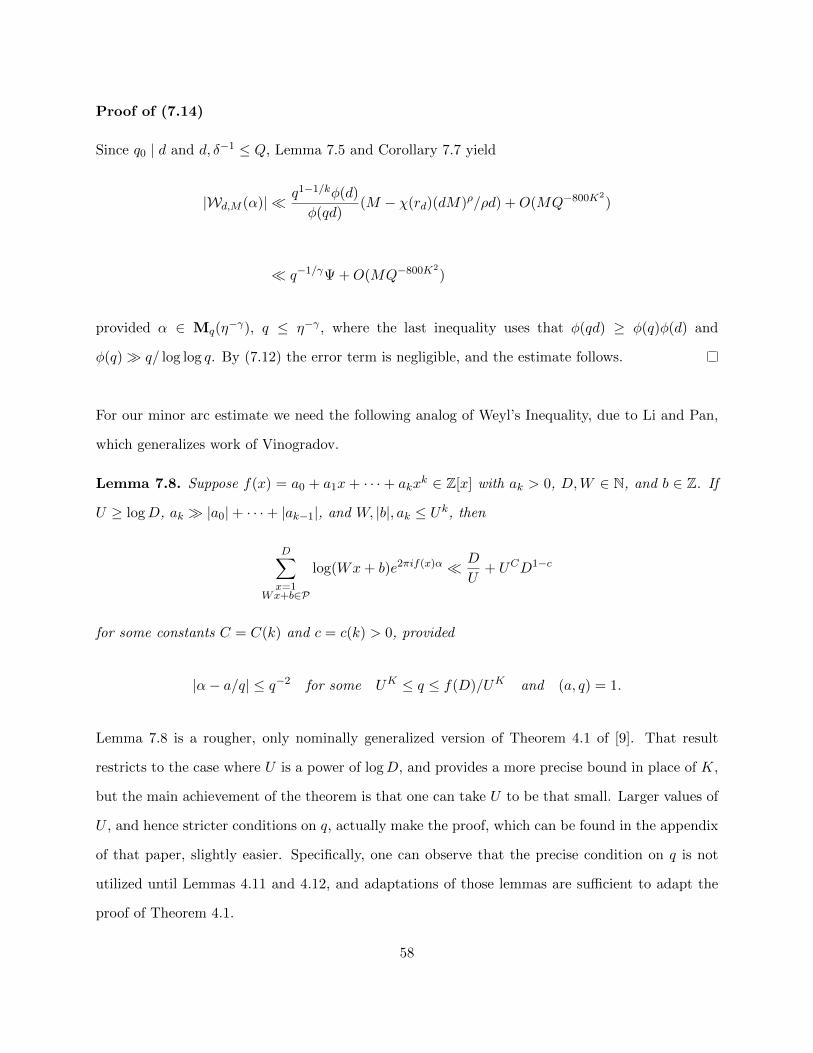
Proof of (7.14)
Since q0 | d and d, δ−1 ≤ Q, Lemma 7.5 and Corollary 7.7 yield
|Wd,M (α)| � q1−1/kφ(d)
φ(qd)(M − χ(rd)(dM)ρ/ρd) +O(MQ−800K2
)
� q−1/γΨ +O(MQ−800K2)
provided α ∈ Mq(η−γ), q ≤ η−γ , where the last inequality uses that φ(qd) ≥ φ(q)φ(d) and
φ(q)� q/ log log q. By (7.12) the error term is negligible, and the estimate follows.
For our minor arc estimate we need the following analog of Weyl’s Inequality, due to Li and Pan,
which generalizes work of Vinogradov.
Lemma 7.8. Suppose f(x) = a0 + a1x+ · · ·+ akxk ∈ Z[x] with ak > 0, D,W ∈ N, and b ∈ Z. If
U ≥ logD, ak � |a0|+ · · ·+ |ak−1|, and W, |b|, ak ≤ Uk, then
D∑x=1
Wx+b∈P
log(Wx+ b)e2πif(x)α � D
U+ UCD1−c
for some constants C = C(k) and c = c(k) > 0, provided
|α− a/q| ≤ q−2 for some UK ≤ q ≤ f(D)/UK and (a, q) = 1.
Lemma 7.8 is a rougher, only nominally generalized version of Theorem 4.1 of [9]. That result
restricts to the case where U is a power of logD, and provides a more precise bound in place of K,
but the main achievement of the theorem is that one can take U to be that small. Larger values of
U , and hence stricter conditions on q, actually make the proof, which can be found in the appendix
of that paper, slightly easier. Specifically, one can observe that the precise condition on q is not
utilized until Lemmas 4.11 and 4.12, and adaptations of those lemmas are sufficient to adapt the
proof of Theorem 4.1.
58
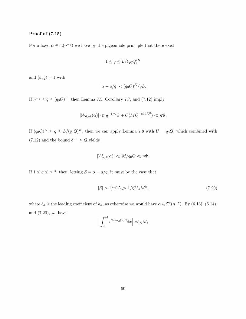
Proof of (7.15)
For a fixed α ∈ m(η−γ) we have by the pigeonhole principle that there exist
1 ≤ q ≤ L/(q0Q)K
and (a, q) = 1 with
|α− a/q| < (q0Q)K/qL.
If η−γ ≤ q ≤ (q0Q)K , then Lemma 7.5, Corollary 7.7, and (7.12) imply
|Wd,M (α)| � q−1/γΨ +O(MQ−800K2)� ηΨ.
If (q0Q)K ≤ q ≤ L/(q0Q)K , then we can apply Lemma 7.8 with U = q0Q, which combined with
(7.12) and the bound δ−1 ≤ Q yields
|Wd,Mα)| �M/q0Q� ηΨ.
If 1 ≤ q ≤ η−2, then, letting β = α− a/q, it must be the case that
|β| > 1/ηγL� 1/ηγbdMk, (7.20)
where bd is the leading coefficient of hd, as otherwise we would have α ∈M(η−γ). By (6.13), (6.14),
and (7.20), we have ∣∣∣ ∫ M
0e2πihd(x)βdx
∣∣∣� ηM,
59
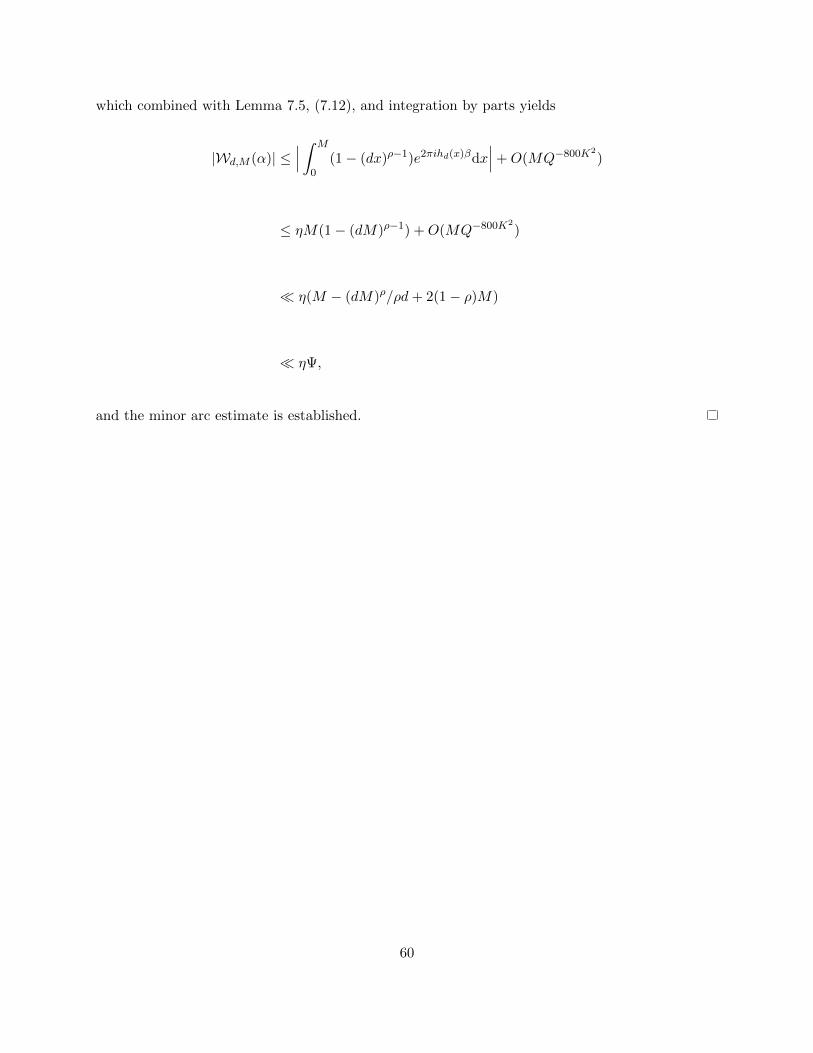
which combined with Lemma 7.5, (7.12), and integration by parts yields
|Wd,M (α)| ≤∣∣∣ ∫ M
0(1− (dx)ρ−1)e2πihd(x)βdx
∣∣∣+O(MQ−800K2)
≤ ηM(1− (dM)ρ−1) +O(MQ−800K2)
� η(M − (dM)ρ/ρd+ 2(1− ρ)M)
� ηΨ,
and the minor arc estimate is established.
60
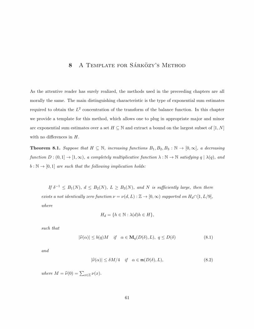
8 A Template for Sarkozy’s Method
As the attentive reader has surely realized, the methods used in the preceeding chapters are all
morally the same. The main distinguishing characteristic is the type of exponential sum estimates
required to obtain the L2 concentration of the transform of the balance function. In this chapter
we provide a template for this method, which allows one to plug in appropriate major and minor
arc exponential sum estimates over a set H ⊆ N and extract a bound on the largest subset of [1, N ]
with no differences in H.
Theorem 8.1. Suppose that H ⊆ N, increasing functions B1, B2, B3 : N → [0,∞], a decreasing
function D : (0, 1]→ [1,∞), a completely multiplicative function λ : N→ N satisfying q | λ(q), and
b : N→ [0, 1] are such that the following implication holds:
If δ−1 ≤ B1(N), d ≤ B2(N), L ≥ B3(N), and N is sufficiently large, then there
exists a not identically zero function ν = ν(d, L) : Z→ [0,∞) supported on Hd∩[1, L/9],
where
Hd = {h ∈ N : λ(d)h ∈ H},
such that
|ν(α)| ≤ b(q)M if α ∈Mq(D(δ), L), q ≤ D(δ) (8.1)
and
|ν(α)| ≤ δM/4 if α ∈ m(D(δ), L), (8.2)
where M = ν(0) =∑
x∈Z ν(x).
61
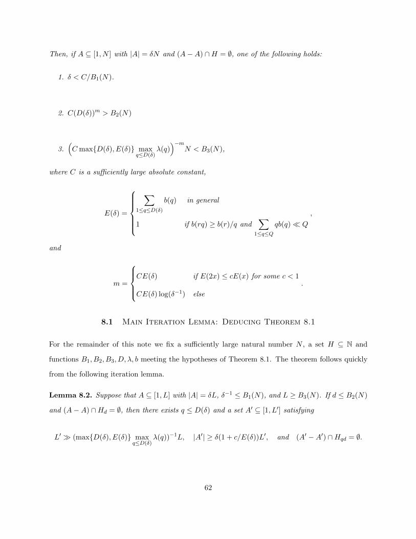
Then, if A ⊆ [1, N ] with |A| = δN and (A−A) ∩H = ∅, one of the following holds:
1. δ < C/B1(N).
2. C(D(δ))m > B2(N)
3.(C max{D(δ), E(δ)} max
q≤D(δ)λ(q)
)−mN < B3(N),
where C is a sufficiently large absolute constant,
E(δ) =
∑
1≤q≤D(δ)
b(q) in general
1 if b(rq) ≥ b(r)/q and∑
1≤q≤Qqb(q)� Q
,
and
m =
CE(δ) if E(2x) ≤ cE(x) for some c < 1
CE(δ) log(δ−1) else
.
8.1 Main Iteration Lemma: Deducing Theorem 8.1
For the remainder of this note we fix a sufficiently large natural number N , a set H ⊆ N and
functions B1, B2, B3, D, λ, b meeting the hypotheses of Theorem 8.1. The theorem follows quickly
from the following iteration lemma.
Lemma 8.2. Suppose that A ⊆ [1, L] with |A| = δL, δ−1 ≤ B1(N), and L ≥ B3(N). If d ≤ B2(N)
and (A−A) ∩Hd = ∅, then there exists q ≤ D(δ) and a set A′ ⊆ [1, L′] satisfying
L′ � (max{D(δ), E(δ)} maxq≤D(δ)
λ(q))−1L, |A′| ≥ δ(1 + c/E(δ))L′, and (A′ −A′) ∩Hqd = ∅.
62
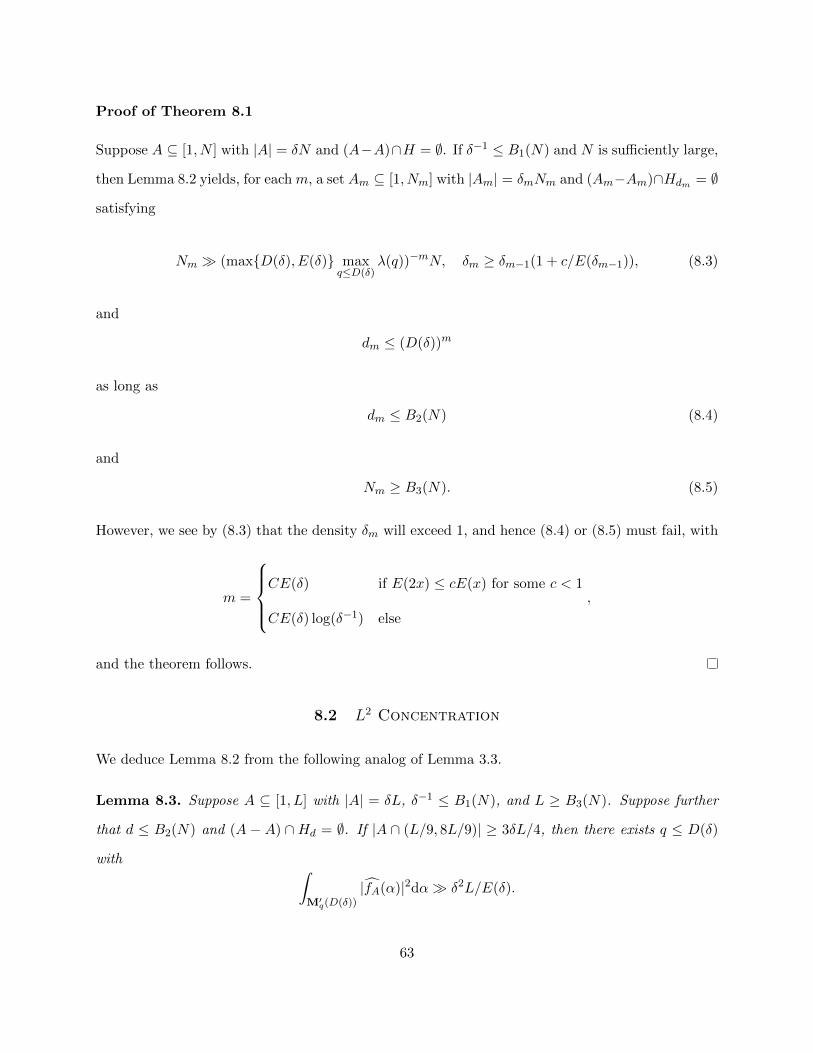
Proof of Theorem 8.1
Suppose A ⊆ [1, N ] with |A| = δN and (A−A)∩H = ∅. If δ−1 ≤ B1(N) and N is sufficiently large,
then Lemma 8.2 yields, for each m, a set Am ⊆ [1, Nm] with |Am| = δmNm and (Am−Am)∩Hdm = ∅
satisfying
Nm � (max{D(δ), E(δ)} maxq≤D(δ)
λ(q))−mN, δm ≥ δm−1(1 + c/E(δm−1)), (8.3)
and
dm ≤ (D(δ))m
as long as
dm ≤ B2(N) (8.4)
and
Nm ≥ B3(N). (8.5)
However, we see by (8.3) that the density δm will exceed 1, and hence (8.4) or (8.5) must fail, with
m =
CE(δ) if E(2x) ≤ cE(x) for some c < 1
CE(δ) log(δ−1) else
,
and the theorem follows.
8.2 L2 Concentration
We deduce Lemma 8.2 from the following analog of Lemma 3.3.
Lemma 8.3. Suppose A ⊆ [1, L] with |A| = δL, δ−1 ≤ B1(N), and L ≥ B3(N). Suppose further
that d ≤ B2(N) and (A − A) ∩Hd = ∅. If |A ∩ (L/9, 8L/9)| ≥ 3δL/4, then there exists q ≤ D(δ)
with ∫M′q(D(δ))
|fA(α)|2dα� δ2L/E(δ).
63
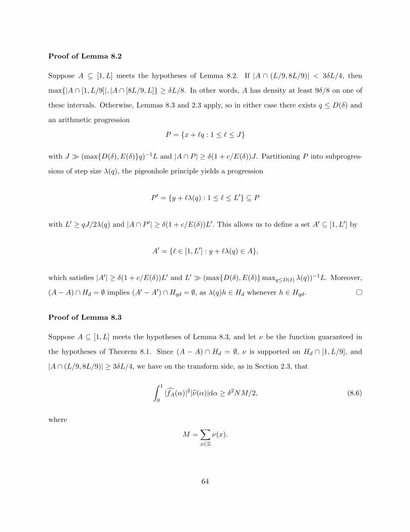
Proof of Lemma 8.2
Suppose A ⊆ [1, L] meets the hypotheses of Lemma 8.2. If |A ∩ (L/9, 8L/9)| < 3δL/4, then
max{|A ∩ [1, L/9]|, |A ∩ [8L/9, L]} ≥ δL/8. In other words, A has density at least 9δ/8 on one of
these intervals. Otherwise, Lemmas 8.3 and 2.3 apply, so in either case there exists q ≤ D(δ) and
an arithmetic progression
P = {x+ `q : 1 ≤ ` ≤ J}
with J � (max{D(δ), E(δ)}q)−1L and |A ∩ P | ≥ δ(1 + c/E(δ))J . Partitioning P into subprogres-
sions of step size λ(q), the pigeonhole principle yields a progression
P ′ = {y + `λ(q) : 1 ≤ ` ≤ L′} ⊆ P
with L′ ≥ qJ/2λ(q) and |A ∩ P ′| ≥ δ(1 + c/E(δ))L′. This allows us to define a set A′ ⊆ [1, L′] by
A′ = {` ∈ [1, L′] : y + `λ(q) ∈ A},
which satisfies |A′| ≥ δ(1 + c/E(δ))L′ and L′ � (max{D(δ), E(δ)}maxq≤D(δ) λ(q))−1L. Moreover,
(A−A) ∩Hd = ∅ implies (A′ −A′) ∩Hqd = ∅, as λ(q)h ∈ Hd whenever h ∈ Hqd.
Proof of Lemma 8.3
Suppose A ⊆ [1, L] meets the hypotheses of Lemma 8.3, and let ν be the function guaranteed in
the hypotheses of Theorem 8.1. Since (A − A) ∩ Hd = ∅, ν is supported on Hd ∩ [1, L/9], and
|A ∩ (L/9, 8L/9)| ≥ 3δL/4, we have on the transform side, as in Section 2.3, that
∫ 1
0|fA(α)|2|ν(α)|dα ≥ δ2NM/2, (8.6)
where
M =∑x∈Z
ν(x).
64
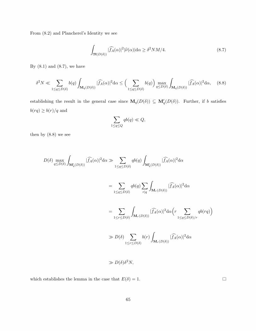
From (8.2) and Plancherel’s Identity we see
∫M(D(δ))
|fA(α)|2|ν(α)|dα ≥ δ2NM/4. (8.7)
By (8.1) and (8.7), we have
δ2N �∑
1≤q≤D(δ)
b(q)
∫Mq(D(δ))
|fA(α)|2dα ≤( ∑
1≤q≤D(δ)
b(q))
maxq≤D(δ)
∫Mq(D(δ))
|fA(α)|2dα, (8.8)
establishing the result in the general case since Mq(D(δ)) ⊆ M′q(D(δ)). Further, if b satisfies
b(rq) ≥ b(r)/q and ∑1≤q≤Q
qb(q)� Q,
then by (8.8) we see
D(δ) maxq≤D(δ)
∫M′q(D(δ))
|fA(α)|2dα�∑
1≤q≤D(δ)
qb(q)
∫M′q(D(δ))
|fA(α)|2dα
=∑
1≤q≤D(δ)
qb(q)∑r|q
∫Mr(D(δ))
|fA(α)|2dα
=∑
1≤r≤D(δ)
∫Mr(D(δ))
|fA(α)|2dα(r
∑1≤q≤D(δ)/r
qb(rq))
� D(δ)∑
1≤r≤D(δ)
b(r)
∫Mr(D(δ))
|fA(α)|2dα
� D(δ)δ2N,
which establishes the lemma in the case that E(δ) = 1.
65
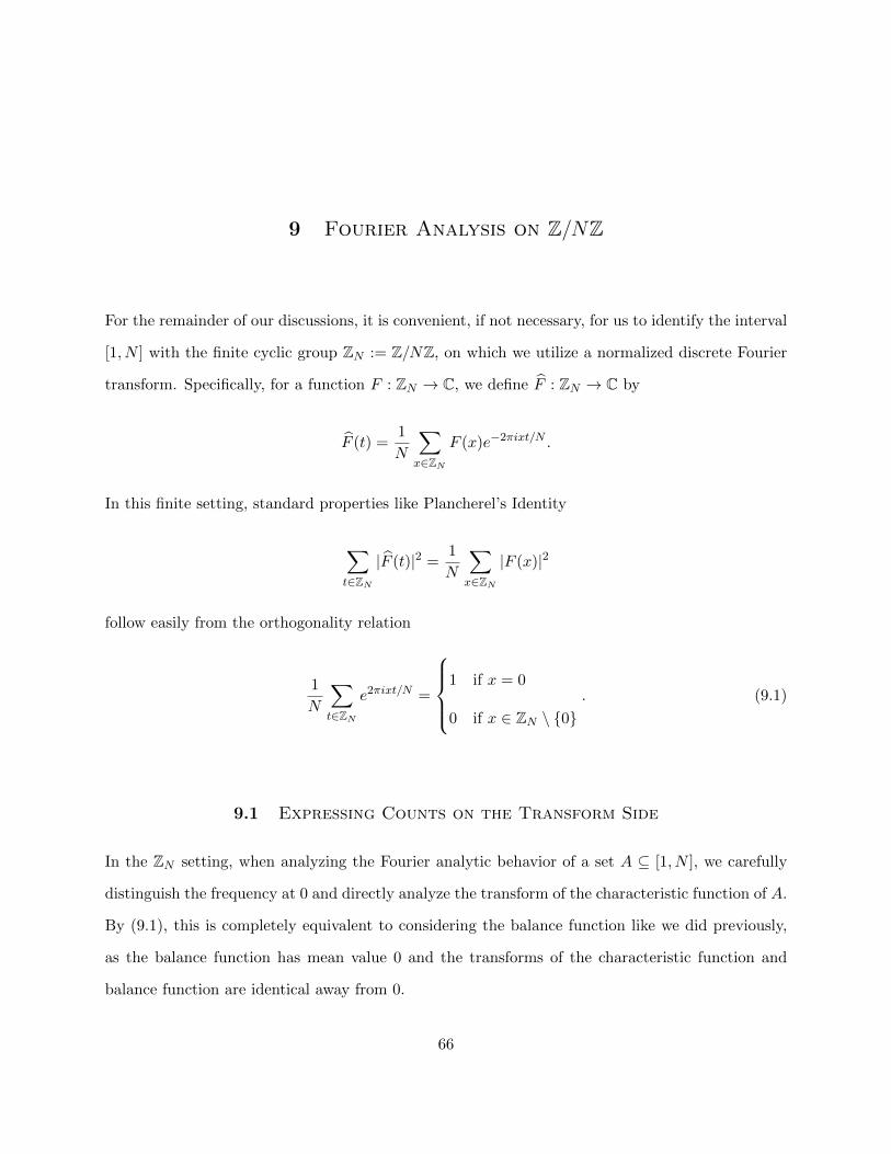
9 Fourier Analysis on Z/NZ
For the remainder of our discussions, it is convenient, if not necessary, for us to identify the interval
[1, N ] with the finite cyclic group ZN := Z/NZ, on which we utilize a normalized discrete Fourier
transform. Specifically, for a function F : ZN → C, we define F : ZN → C by
F (t) =1
N
∑x∈ZN
F (x)e−2πixt/N .
In this finite setting, standard properties like Plancherel’s Identity
∑t∈ZN
|F (t)|2 =1
N
∑x∈ZN
|F (x)|2
follow easily from the orthogonality relation
1
N
∑t∈ZN
e2πixt/N =
1 if x = 0
0 if x ∈ ZN \ {0}. (9.1)
9.1 Expressing Counts on the Transform Side
In the ZN setting, when analyzing the Fourier analytic behavior of a set A ⊆ [1, N ], we carefully
distinguish the frequency at 0 and directly analyze the transform of the characteristic function of A.
By (9.1), this is completely equivalent to considering the balance function like we did previously,
as the balance function has mean value 0 and the transforms of the characteristic function and
balance function are identical away from 0.
66
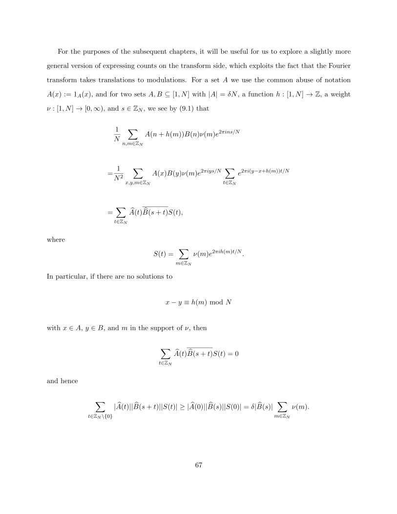
For the purposes of the subsequent chapters, it will be useful for us to explore a slightly more
general version of expressing counts on the transform side, which exploits the fact that the Fourier
transform takes translations to modulations. For a set A we use the common abuse of notation
A(x) := 1A(x), and for two sets A,B ⊆ [1, N ] with |A| = δN , a function h : [1, N ] → Z, a weight
ν : [1, N ]→ [0,∞), and s ∈ ZN , we see by (9.1) that
1
N
∑n,m∈ZN
A(n+ h(m))B(n)ν(m)e2πins/N
=1
N2
∑x,y,m∈ZN
A(x)B(y)ν(m)e2πiys/N∑t∈ZN
e2πi(y−x+h(m))t/N
=∑t∈ZN
A(t)B(s+ t)S(t),
where
S(t) =∑m∈ZN
ν(m)e2πih(m)t/N .
In particular, if there are no solutions to
x− y ≡ h(m) mod N
with x ∈ A, y ∈ B, and m in the support of ν, then
∑t∈ZN
A(t)B(s+ t)S(t) = 0
and hence
∑t∈ZN\{0}
|A(t)||B(s+ t)||S(t)| ≥ |A(0)||B(s)||S(0)| = δ|B(s)|∑m∈ZN
ν(m).
67
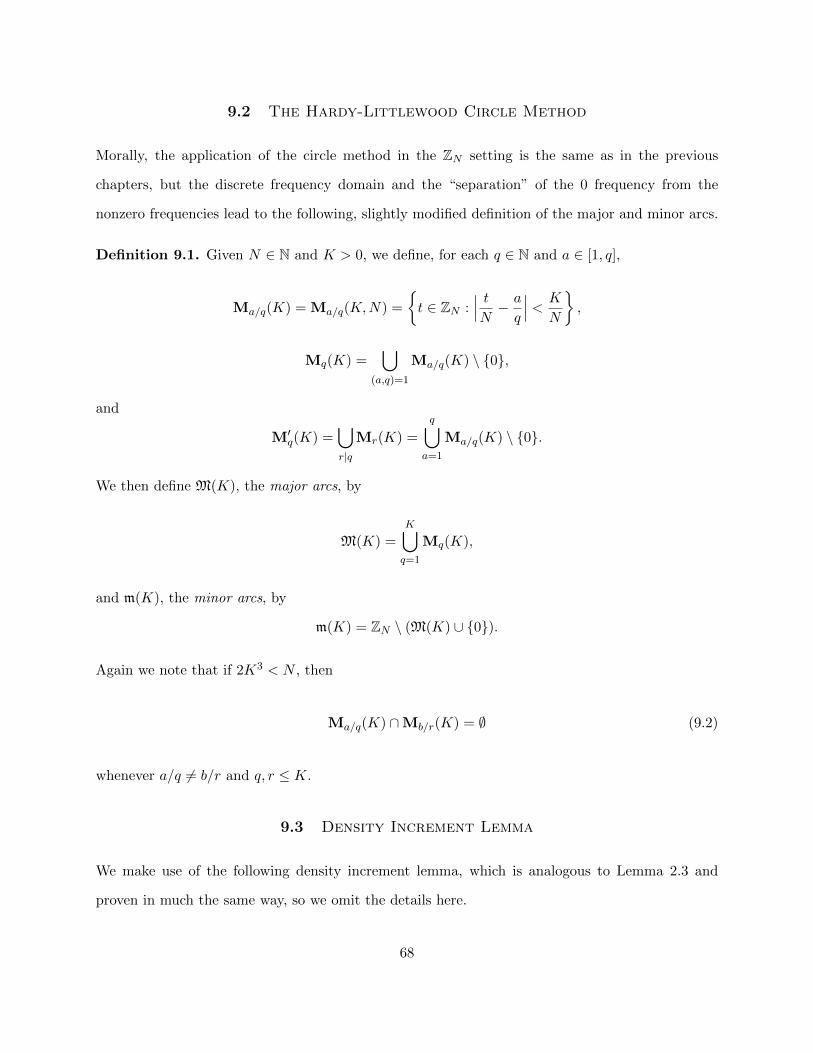
9.2 The Hardy-Littlewood Circle Method
Morally, the application of the circle method in the ZN setting is the same as in the previous
chapters, but the discrete frequency domain and the “separation” of the 0 frequency from the
nonzero frequencies lead to the following, slightly modified definition of the major and minor arcs.
Definition 9.1. Given N ∈ N and K > 0, we define, for each q ∈ N and a ∈ [1, q],
Ma/q(K) = Ma/q(K,N) =
{t ∈ ZN :
∣∣∣ tN− a
q
∣∣∣ < K
N
},
Mq(K) =⋃
(a,q)=1
Ma/q(K) \ {0},
and
M′q(K) =
⋃r|q
Mr(K) =
q⋃a=1
Ma/q(K) \ {0}.
We then define M(K), the major arcs, by
M(K) =
K⋃q=1
Mq(K),
and m(K), the minor arcs, by
m(K) = ZN \ (M(K) ∪ {0}).
Again we note that if 2K3 < N , then
Ma/q(K) ∩Mb/r(K) = ∅ (9.2)
whenever a/q 6= b/r and q, r ≤ K.
9.3 Density Increment Lemma
We make use of the following density increment lemma, which is analogous to Lemma 2.3 and
proven in much the same way, so we omit the details here.
68
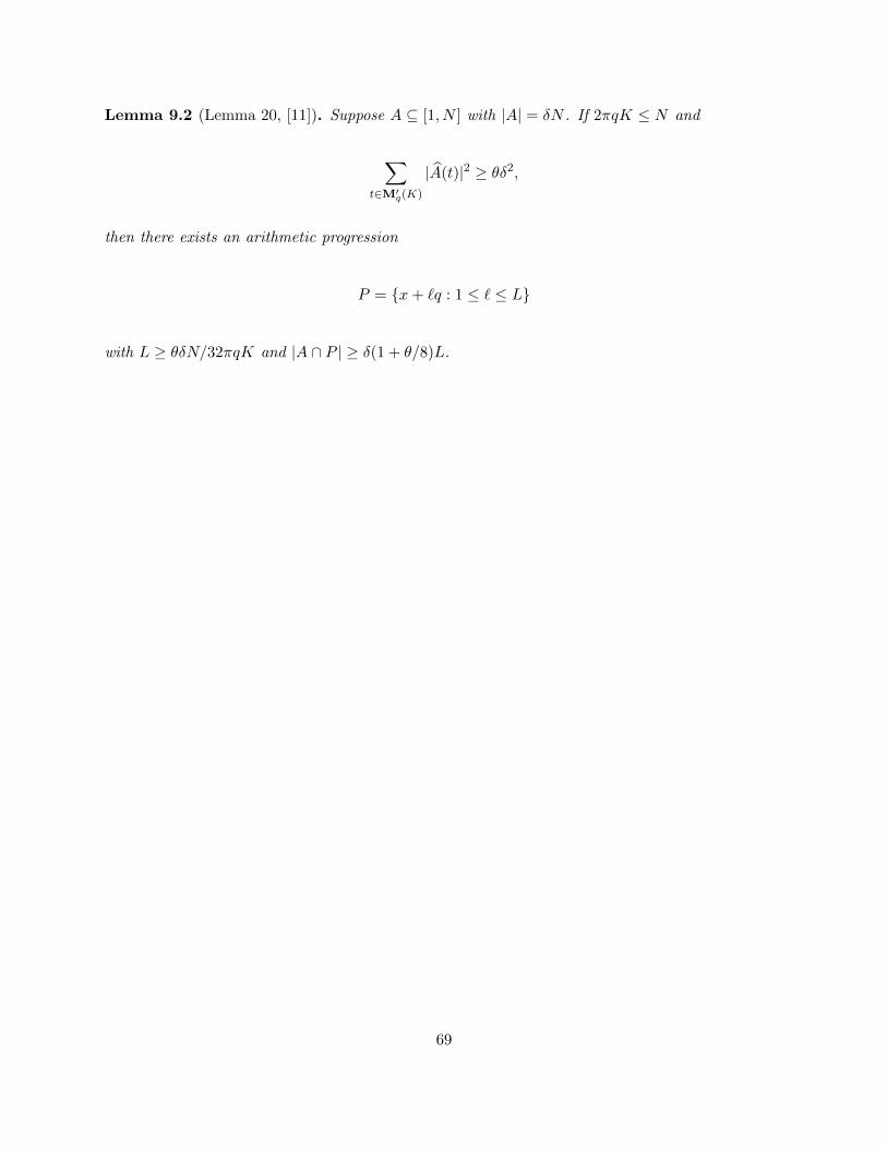
Lemma 9.2 (Lemma 20, [11]). Suppose A ⊆ [1, N ] with |A| = δN . If 2πqK ≤ N and
∑t∈M′q(K)
|A(t)|2 ≥ θδ2,
then there exists an arithmetic progression
P = {x+ `q : 1 ≤ ` ≤ L}
with L ≥ θδN/32πqK and |A ∩ P | ≥ δ(1 + θ/8)L.
69
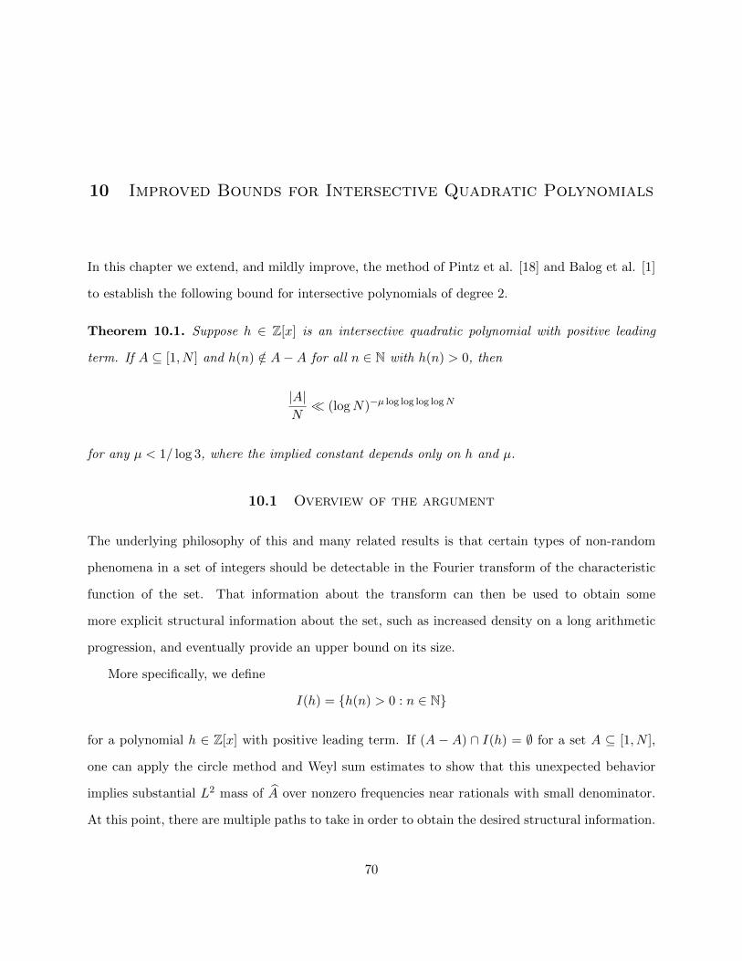
10 Improved Bounds for Intersective Quadratic Polynomials
In this chapter we extend, and mildly improve, the method of Pintz et al. [18] and Balog et al. [1]
to establish the following bound for intersective polynomials of degree 2.
Theorem 10.1. Suppose h ∈ Z[x] is an intersective quadratic polynomial with positive leading
term. If A ⊆ [1, N ] and h(n) /∈ A−A for all n ∈ N with h(n) > 0, then
|A|N� (logN)−µ log log log logN
for any µ < 1/ log 3, where the implied constant depends only on h and µ.
10.1 Overview of the argument
The underlying philosophy of this and many related results is that certain types of non-random
phenomena in a set of integers should be detectable in the Fourier transform of the characteristic
function of the set. That information about the transform can then be used to obtain some
more explicit structural information about the set, such as increased density on a long arithmetic
progression, and eventually provide an upper bound on its size.
More specifically, we define
I(h) = {h(n) > 0 : n ∈ N}
for a polynomial h ∈ Z[x] with positive leading term. If (A − A) ∩ I(h) = ∅ for a set A ⊆ [1, N ],
one can apply the circle method and Weyl sum estimates to show that this unexpected behavior
implies substantial L2 mass of A over nonzero frequencies near rationals with small denominator.
At this point, there are multiple paths to take in order to obtain the desired structural information.
70
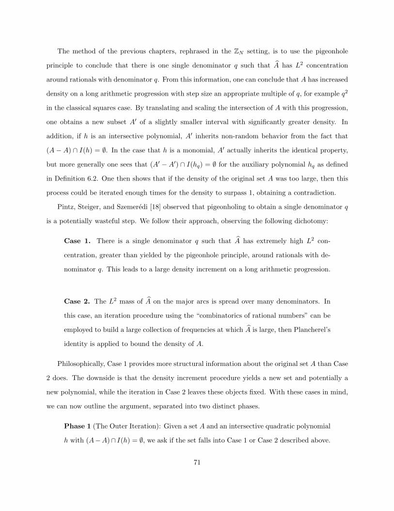
The method of the previous chapters, rephrased in the ZN setting, is to use the pigeonhole
principle to conclude that there is one single denominator q such that A has L2 concentration
around rationals with denominator q. From this information, one can conclude that A has increased
density on a long arithmetic progression with step size an appropriate multiple of q, for example q2
in the classical squares case. By translating and scaling the intersection of A with this progression,
one obtains a new subset A′ of a slightly smaller interval with significantly greater density. In
addition, if h is an intersective polynomial, A′ inherits non-random behavior from the fact that
(A − A) ∩ I(h) = ∅. In the case that h is a monomial, A′ actually inherits the identical property,
but more generally one sees that (A′ − A′) ∩ I(hq) = ∅ for the auxiliary polynomial hq as defined
in Definition 6.2. One then shows that if the density of the original set A was too large, then this
process could be iterated enough times for the density to surpass 1, obtaining a contradiction.
Pintz, Steiger, and Szemeredi [18] observed that pigeonholing to obtain a single denominator q
is a potentially wasteful step. We follow their approach, observing the following dichotomy:
Case 1. There is a single denominator q such that A has extremely high L2 con-
centration, greater than yielded by the pigeonhole principle, around rationals with de-
nominator q. This leads to a large density increment on a long arithmetic progression.
Case 2. The L2 mass of A on the major arcs is spread over many denominators. In
this case, an iteration procedure using the “combinatorics of rational numbers” can be
employed to build a large collection of frequencies at which A is large, then Plancherel’s
identity is applied to bound the density of A.
Philosophically, Case 1 provides more structural information about the original set A than Case
2 does. The downside is that the density increment procedure yields a new set and potentially a
new polynomial, while the iteration in Case 2 leaves these objects fixed. With these cases in mind,
we can now outline the argument, separated into two distinct phases.
Phase 1 (The Outer Iteration): Given a set A and an intersective quadratic polynomial
h with (A−A)∩ I(h) = ∅, we ask if the set falls into Case 1 or Case 2 described above.
71
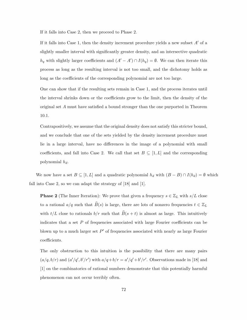
If it falls into Case 2, then we proceed to Phase 2.
If it falls into Case 1, then the density increment procedure yields a new subset A′ of a
slightly smaller interval with significantly greater density, and an intersective quadratic
hq with slightly larger coefficients and (A′ − A′) ∩ I(hq) = ∅. We can then iterate this
process as long as the resulting interval is not too small, and the dichotomy holds as
long as the coefficients of the corresponding polynomial are not too large.
One can show that if the resulting sets remain in Case 1, and the process iterates until
the interval shrinks down or the coefficients grow to the limit, then the density of the
original set A must have satisfied a bound stronger than the one purported in Theorem
10.1.
Contrapositively, we assume that the original density does not satisfy this stricter bound,
and we conclude that one of the sets yielded by the density increment procedure must
lie in a large interval, have no differences in the image of a polynomial with small
coefficients, and fall into Case 2. We call that set B ⊆ [1, L] and the corresponding
polynomial hd.
We now have a set B ⊆ [1, L] and a quadratic polynomial hd with (B − B) ∩ I(hd) = ∅ which
fall into Case 2, so we can adapt the strategy of [18] and [1].
Phase 2 (The Inner Iteration): We prove that given a frequency s ∈ ZL with s/L close
to a rational a/q such that B(s) is large, there are lots of nonzero frequencies t ∈ ZL
with t/L close to rationals b/r such that B(s + t) is almost as large. This intuitively
indicates that a set P of frequencies associated with large Fourier coefficients can be
blown up to a much larger set P ′ of frequencies associated with nearly as large Fourier
coefficients.
The only obstruction to this intuition is the possibility that there are many pairs
(a/q, b/r) and (a′/q′, b′/r′) with a/q+b/r = a′/q′+b′/r′. Observations made in [18] and
[1] on the combinatorics of rational numbers demonstrate that this potentially harmful
phenomenon can not occur terribly often.
72
Starting with the trivially large Fourier coefficient at 0, this process is applied as long
as certain parameters are not too large, and the number of iterations is ultimately
limited by the growth of the divisor function. Once the iteration is exhausted, we use
the resulting set of large Fourier coefficients and Plancherel’s Identity to get the upper
bound on the density of B, which is by construction larger than the density of the
original set A, claimed in Theorem 10.1.
10.2 Reduction of Theorem 10.1 to Two Lemmas
To make the strategy outlined in Section 10.1 precise, we fix a natural number N , an intersective
quadratic polynomial h ∈ Z[x] with positive leading term, and a set A ⊆ [1, N ] with |A| = δN and
(A − A) ∩ I(h) = ∅. We fix p-adic integer roots zp of h for each prime p, which determine roots
rd ∈ (−d, 0] of h modulo each d ∈ N, and we let the function λ and the auxiliary polynomials hd
be as in Definition 6.2. We also fix an arbitrary ε > 0, set Z = (logN)ε log log logN , and we prove
Theorem 10.1 with µ = (1− 11ε)/ log 3.
Lemma 10.2. If
δ ≥ e−(logN)ε/8 , (10.1)
then there exists B ⊆ [1, L] satisfying L ≥ N .99, |B|/L = σ ≥ δ, and (B − B) ∩ I(hd) = ∅ with
d ≤ N .01. Further, B satisfies |B ∩ [1, L/2]| ≥ σL/3 and
maxq≤Z
∑t∈Mq(Z)
|B(t)|2 ≤ σ2(logN)−1+ε. (10.2)
We note that e−(logN)ε/8 � (logN)− log log log logN . In particular, if hypothesis (10.1) is not
satisfied, then Theorem 10.1 is already more than true. The next lemma corresponds to the
iteration scheme in which a set of large Fourier coefficients from distinct major arcs is blown up in
such a way that the relative growth of the size of the set is much greater than the relative loss of
pointwise mass.
73
Lemma 10.3. Suppose B ⊆ [1, L] with |B| = σL is as in the conclusion of Lemma 10.2, let
B1 = B ∩ [1, L/2], and suppose σ ≥ Z−1/6. Given U, V,K ∈ N with max{U, V,K} ≤ Z1/6 and a set
P ⊆
t ∈V⋃q=1
Mq(K) ∪ {0} : |B1(t)| ≥ σ
U
satisfying
|P ∩Ma,q(K)| ≤ 1 whenever q ≤ V, (10.3)
there exist U ′, V ′,K ′ ∈ N with max{U ′, V ′,K ′} � (max{U, V,K})3σ−5/2 and a set
P ′ ⊆
t ∈V ′⋃q=1
Mq(K′) ∪ {0} : |B1(t)| ≥ σ
U ′
(10.4)
satisfying
|P ′ ∩Ma,q(K′)| ≤ 1 whenever q ≤ V ′ (10.5)
and
|P ′|(U ′)2
≥ |P |U2
(logN)1−10ε. (10.6)
Proof of Theorem 10.1
In order to prove Theorem 10.1, we can assume that
δ ≥ (logN)− log log log logN .
Therefore, Lemma 10.2 produces a set B of density σ ≥ δ with the stipulated properties, and we set
P0 = {0}, U0 = 3, and V0 = K0 = 1. Lemma 10.3 then yields, for each n, a set Pn with parameters
Un, Vn,Kn such that
max{Un, Vn,Kn} ≤ (logN)3n+1 log log log logN
and
1
σ≥ 1
σ2
∑t∈Pn
|B1(t)|2 ≥ |Pn|U2n
� (logN)n(1−10ε),
74
where the left-hand inequality comes from Plancherel’s Identity, as long as max{Un, Vn,Kn} ≤ Z1/6.
This holds with n = (1 − ε)(log log log logN)/ log 3, as 3n+1 ≤ (log log logN)1−ε/2, and Theorem
10.1 follows.
10.3 The Outer Iteration I
We deduce Lemma 10.2 from the following density increment lemma which, after partitioning a
progression of step size q into progressions of step size λ(q), follows immediately from Lemma 9.2
and Proposition 6.3.
Lemma 10.4. Suppose B ⊆ [1, L] with |B| = σL and (B −B) ∩ I(hd) = ∅. If L ≥ Z4 and
∑t∈Mq(Z)
|B(t)|2 ≥ σ2(logN)−1+ε, (10.7)
for some q ≤ Z, then there exists B′ ⊆ [1, L′] satisfying L′ � σL/Z4, (B′ −B′) ∩ I(hqd) = ∅, and
|B′|/L′ ≥ σ(1 + (logN)−1+ε/8).
Proof of Lemma 10.2
Setting A0=A, N0 = N , δ0 = δ, and d0 = 1, we iteratively apply Lemma 10.4. This yields, for each
k, a set Ak ⊆ [1, Nk] with |Ak| = δkNk and (Ak −Ak) ∩ I(hdk) = ∅ satisfying
Nk ≥ (cδ/Z4)kN, δk ≥ δk−1(1 + (logN)−1+ε/8), and dk ≤ Zk (10.8)
as long as Nk ≥ Z4 and either
maxq≤Z
∑t∈Mq(Z)
|Ak(t)|2 ≥ δ2k(logN)−1+ε (10.9)
or |Ak ∩ [1, Nk/2]| < δkNk/3, as the latter condition implies Ak has density at least 3δk/2 on the
interval (Nk/2, Nk].
75
We see that by (10.1) and (10.8), the density δk will exceed 1 after
16 log(δ−1)(logN)1−ε ≤ (logN)1−ε/2
steps, hence Nk < Z4 or (10.9) fails and |Ak ∩ [1, Nk/2]| ≥ δkNk/3 for some
k ≤ (logN)1−ε/2. (10.10)
However, we see that (10.1), (10.8), and (10.10) imply
Nk ≥ N(e−(logN)ε/4)(logN)1−ε/2 ≥ Ne−(logN)1−ε/4 ≥ N .99,
so we set B = Ak, L = Nk, σ = δk, and d = dk, and we see further that
d ≤ Z(logN)1−ε/2 ≤ e(logN)1−ε/4 ≤ N .01,
as required.
10.4 The Inner Iteration I
In this section, we let B ⊆ [1, L] and hd ∈ Z[x] be as in the conclusion of Lemma 10.2, we let
B1 = B ∩ [1, L/2], and we assume σ ≥ Z−1/6. We set M =√L/10bd, where bd is the leading
coefficient of hd, and Hd = {n ∈ N : 0 < hd(n) < L/10}, noting by (6.1) that
|Hd 4 [1,M ]| � 1. (10.11)
Proof of Lemma 10.3
Suppose we have a set P with parameters U, V,K as specified in the hypotheses of Lemma 10.3,
and fix an element s ∈ P . Since (B −B) ∩ I(hd) = ∅, we see that there are no solutions to
a− b ≡ hd(m) mod L, a ∈ B, b ∈ B1, m ∈ Hd.
76
On the transform side as in Section 9.1, combined with (10.11), this implies
∑t∈ZL
B(t)B1(s+ t)S(t) =1
LM2
∑n∈ZLm∈Hd
mB(n+ hd(m))B1(n)e2πins/L +O(M−1) = O(M−1),
where
S(t) =1
M2
M∑m=1
me2πihd(m)t/L,
which immediately yields
∑t∈ZL\{0}
|B(t)||B1(s+ t)||S(t)| ≥ |B(0)B1(s)S(0)|+O(M−1) ≥ σ2/8U, (10.12)
since |B1(s)| ≥ σ/U and S(0) ≥ 1/4. Letting η = c0σ/U for a constant c0 > 0, it follows from
traditional Weyl sum estimates that
|S(t)| � q−1/2 min{1, (L|t/L− a/q|)−1} (10.13)
if t ∈Ma/q(η−2), (a, q) = 1, and q ≤ η−2, and
|S(t)| ≤ Cη ≤ σ/16U for all t ∈ m(η−2), (10.14)
provided c0 ≤ 1/16C. We discuss these estimates in more detail in Section 10.5. We have by
(10.14), Cauchy-Schwarz, and Plancherel’s Identity that
∑t∈M(η−2)
|B(t)||B1(t)||S(t)| ≥ σ2/16U. (10.15)
We now wish to assert that we can ignore those frequencies in the major arcs at which the transform
of B or B1 is particularly small. In order to make this precise, we first need to invoke a weighted
version of a well-known estimate on the higher moments of Weyl sums.
77
Specifically, we have that ∑t∈ZL
|S(t)|6 ≤ C, (10.16)
of which we provide a proof in Section 10.5. Choosing a constant 0 < c1 < (64C1/6)−3, where C
comes from (10.16), we define
X ={t ∈M(η−2) : min
{|B(t)|, |B1(s+ t)|
}≤ c1σ
7/2/U3}
and Y = M(η−2) \X. (10.17)
Using Holder’s Inequality to exploit the sixth moment estimate on S, followed by Plancherel’s
Identity, we see that
∑t∈X|B(t)||B1(s+ t)||S(t)| ≤
(∑t∈X|B(t)|6/5|B1(s+ t)|6/5
)5/6( ∑t∈ZL
|S(t)|6)1/6
≤ c1/31 σ7/6
U
( ∑t∈ZL
|B(t)|2 + |B1(s+ t)|2)5/6
· C1/6
≤ σ2/32U,
and hence by (10.15) we have
∑t∈Y|B(t)||B1(s+ t)||S(t)| ≥ σ2/32U. (10.18)
For i, j, k ∈ N, we define
Ri,j,k ={a/q : (a, q) = 1, 2i−1 ≤ q ≤ 2i,
σ
2j≤ max |B(t)| ≤ σ
2j−1,σ
2k≤ max |B1(s+ t)| ≤ σ
2k−1
},
where the maximums are taken over nonzero frequencies t ∈Ma/q(η−2).
78
We see that we have
∑a/q∈Ri,j,k
∑t∈Ma/q(η
−2)\{0}
|B(t)||B1(s+ t)||S(t)| � |Ri,j,k|σ2
2j2kmax
a/q∈Ri,j,k
∑t∈Ma/q(η
−2)
|S(t)|. (10.19)
It follows from (10.13) and the bound U, σ−1 ≤ Z1/6 that if (a, q) = 1 and q ≤ η−2, then
∑t∈Ma/q(η
−2)
|S(t)| � q−1/2 log(Z),
hence by (10.19) we have
∑a/q∈Ri,j,k
∑t∈Ma/q(η
−2)\{0}
|B(t)||B1(s+ t)||S(t)| � |Ri,j,k|σ2
2j2k2−i/2 log(Z). (10.20)
By our definitions, the sets Ri,j,k exhaust Y by taking 1 ≤ 2i ≤ η−2 and 1 ≤ 2j , 2k ≤ U3/c1σ5/2,
a total search space of size � (logZ)3. Therefore, by (10.18) and (10.20) there exist i, j, k in the
above range such that
σ2
U(logZ)3� |Ri,j,k|
σ2
2j2k2−i/2 logZ.
In other words, we can set Vs = 2i, Ws = 2j , and Us = 2k and take an appropriate nonzero
frequency from each of the pairwise disjoint major arcs specified by Ri,j,k to form a set
Ps ⊆
t ∈Vs⋃
q=Vs/2
Mq(η−2) : |B1(s+ t)| ≥ σ
Us
which satisfies
|Ps| �UsWsV
1/2s
U(logZ)4, |Ps ∩Ma,q(η
−2)| ≤ 1 whenever q ≤ Vs, (10.21)
and
maxt∈Ma/q(η
−2)\{0}|B(t)| ≥ σ
Wswhenever q ≤ Vs and Ma/q(η
−2) ∩ Ps 6= ∅, (10.22)
noting by disjointness of the major arcs that a/q ∈ Ri,j,k whenever q ≤ Vs and Ma/q(η−2)∩Ps 6= ∅.
79
Remark. The exponent of 1/2 on Vs in (10.21), which ultimately comes from the exponent on q
in the estimate for the Gauss sum Ghd(a, q) given by Lemma 6.7, is absolutely essential to the
argument. This is exactly the reason for our restriction to quadratic polynomials, as a polynomial
of degree k would yield an exponent of 1/k on Vs. Balog et al. [1] used a sieve in defining their
weighted exponential sum for kth-powers, which resulted in the required “square root cancellation”
in a modified Gauss sum, but this technigue intimately uses algebraic properties of the kth-power
map and does not generalize in any immediate way beyond monomials.
We now observe that there is a subset P ⊆ P with
|P | � |P |/(logZ)3 (10.23)
for which the triple Us,Ws, Vs is the same. We call those common parameters U , W and V , re-
spectively, and we can now foreshadow by asserting that the claimed parameters in the conclusion
of Lemma 10.3 will be U ′ = U , V ′ = V V , and K ′ = K+η−2, which do satisfy the purported bound.
We let
R =
{a
q+b
r: s ∈Ma/q(K) for some s ∈ P and t ∈Mb/r(η
−2) for some t ∈ Ps}.
By taking one frequency s+t associated to each element inR, we form our set P ′, which immediately
satisfies conditions (10.4) and (10.5) from the conclusion of Lemma 10.3. However, the crucial
condition (10.6) on |P ′|, which by construction is equal to |R|, remains to be shown. To this end,
we invoke the work on the combinatorics of rational numbers found in [18] and [1].
80
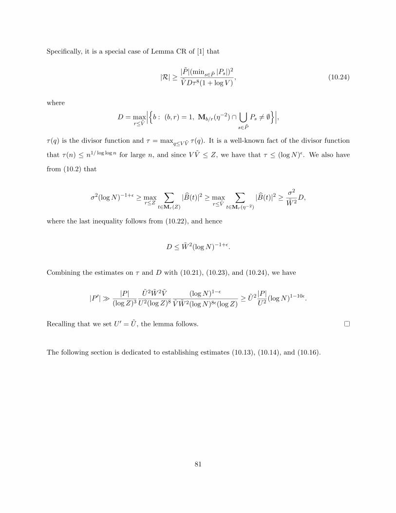
Specifically, it is a special case of Lemma CR of [1] that
|R| ≥|P |(mins∈P |Ps|)
2
V Dτ8(1 + log V ), (10.24)
where
D = maxr≤V
∣∣∣{b : (b, r) = 1, Mb/r(η−2) ∩
⋃s∈P
Ps 6= ∅}∣∣∣,
τ(q) is the divisor function and τ = maxq≤V V τ(q). It is a well-known fact of the divisor function
that τ(n) ≤ n1/ log logn for large n, and since V V ≤ Z, we have that τ ≤ (logN)ε. We also have
from (10.2) that
σ2(logN)−1+ε ≥ maxr≤Z
∑t∈Mr(Z)
|B(t)|2 ≥ maxr≤V
∑t∈Mr(η−2)
|B(t)|2 ≥ σ2
W 2D,
where the last inequality follows from (10.22), and hence
D ≤ W 2(logN)−1+ε.
Combining the estimates on τ and D with (10.21), (10.23), and (10.24), we have
|P ′| � |P |(logZ)3
U2W 2V
U2(logZ)8
(logN)1−ε
V W 2(logN)8ε(logZ)≥ U2 |P |
U2(logN)1−10ε.
Recalling that we set U ′ = U , the lemma follows.
The following section is dedicated to establishing estimates (10.13), (10.14), and (10.16).
81
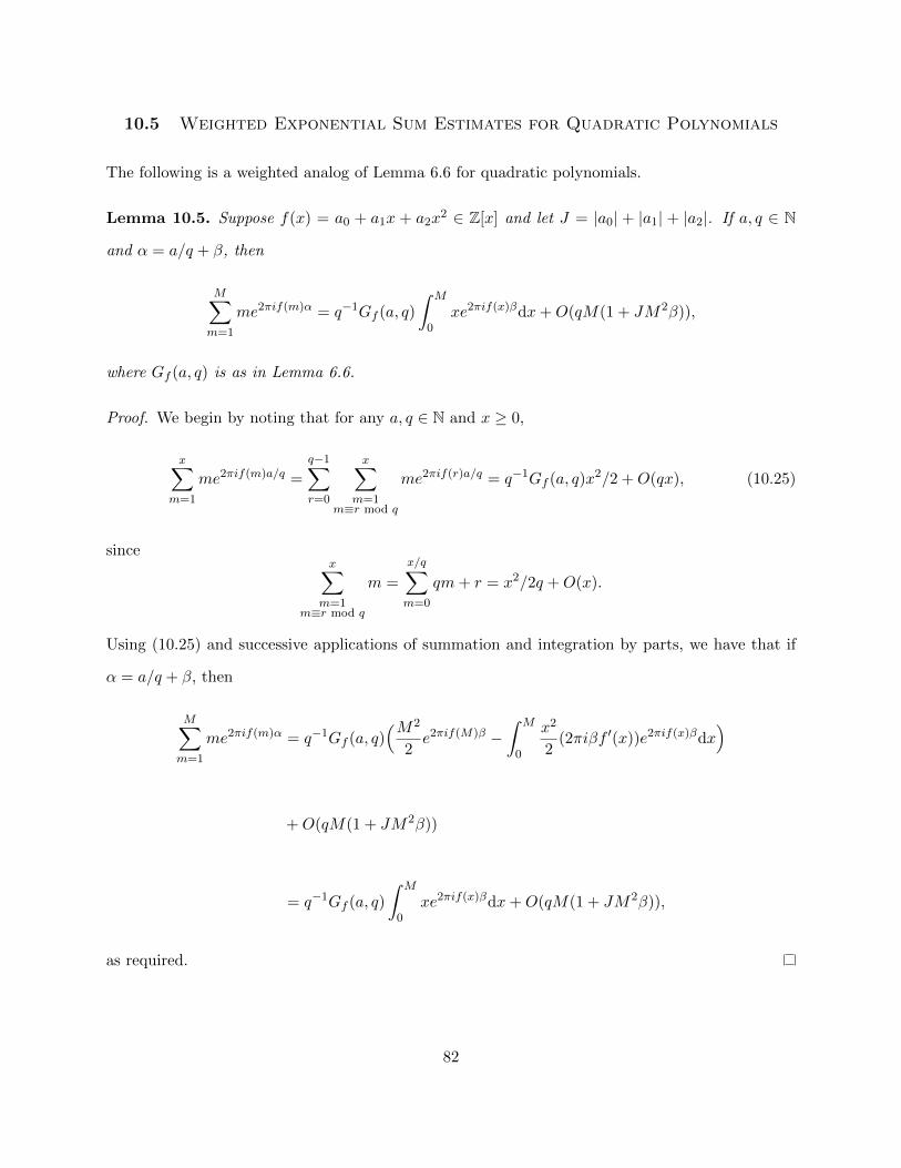
10.5 Weighted Exponential Sum Estimates for Quadratic Polynomials
The following is a weighted analog of Lemma 6.6 for quadratic polynomials.
Lemma 10.5. Suppose f(x) = a0 + a1x + a2x2 ∈ Z[x] and let J = |a0| + |a1| + |a2|. If a, q ∈ N
and α = a/q + β, then
M∑m=1
me2πif(m)α = q−1Gf (a, q)
∫ M
0xe2πif(x)βdx+O(qM(1 + JM2β)),
where Gf (a, q) is as in Lemma 6.6.
Proof. We begin by noting that for any a, q ∈ N and x ≥ 0,
x∑m=1
me2πif(m)a/q =
q−1∑r=0
x∑m=1
m≡r mod q
me2πif(r)a/q = q−1Gf (a, q)x2/2 +O(qx), (10.25)
sincex∑
m=1m≡r mod q
m =
x/q∑m=0
qm+ r = x2/2q +O(x).
Using (10.25) and successive applications of summation and integration by parts, we have that if
α = a/q + β, then
M∑m=1
me2πif(m)α = q−1Gf (a, q)(M2
2e2πif(M)β −
∫ M
0
x2
2(2πiβf ′(x))e2πif(x)βdx
)
+O(qM(1 + JM2β))
= q−1Gf (a, q)
∫ M
0xe2πif(x)βdx+O(qM(1 + JM2β)),
as required.
82
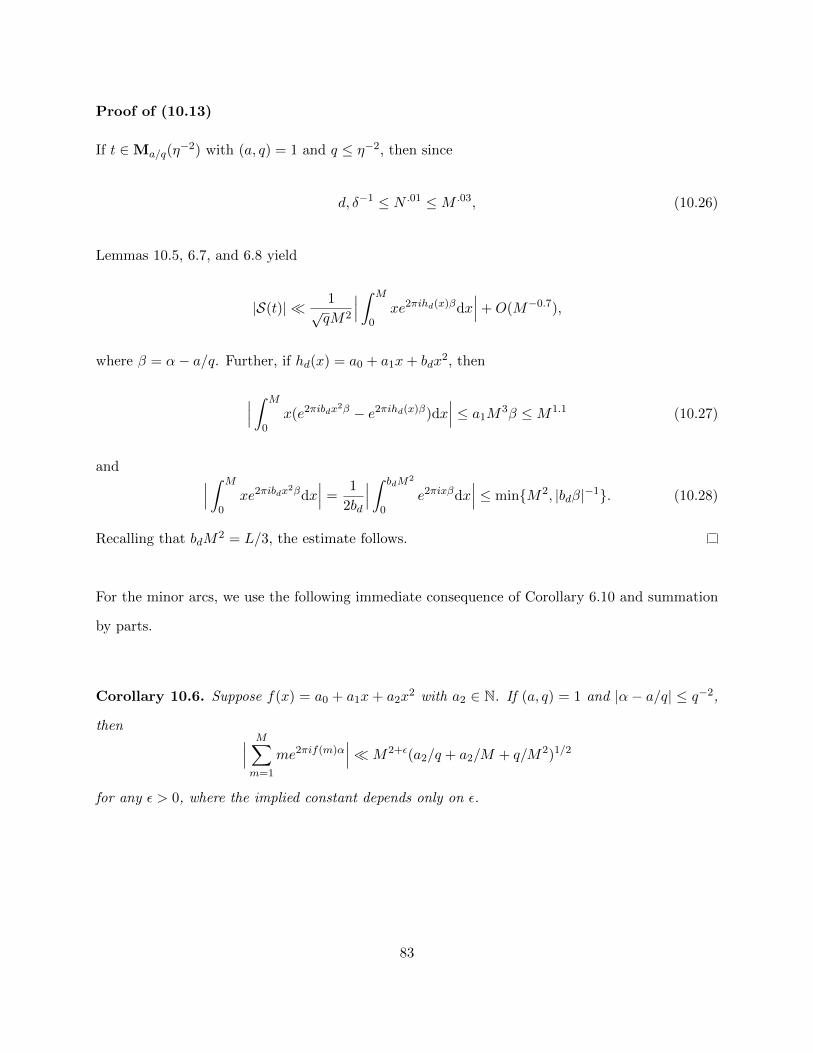
Proof of (10.13)
If t ∈Ma/q(η−2) with (a, q) = 1 and q ≤ η−2, then since
d, δ−1 ≤ N .01 ≤M .03, (10.26)
Lemmas 10.5, 6.7, and 6.8 yield
|S(t)| � 1√qM2
∣∣∣ ∫ M
0xe2πihd(x)βdx
∣∣∣+O(M−0.7),
where β = α− a/q. Further, if hd(x) = a0 + a1x+ bdx2, then
∣∣∣ ∫ M
0x(e2πibdx
2β − e2πihd(x)β)dx∣∣∣ ≤ a1M
3β ≤M1.1 (10.27)
and ∣∣∣ ∫ M
0xe2πibdx
2βdx∣∣∣ =
1
2bd
∣∣∣ ∫ bdM2
0e2πixβdx
∣∣∣ ≤ min{M2, |bdβ|−1}. (10.28)
Recalling that bdM2 = L/3, the estimate follows.
For the minor arcs, we use the following immediate consequence of Corollary 6.10 and summation
by parts.
Corollary 10.6. Suppose f(x) = a0 + a1x+ a2x2 with a2 ∈ N. If (a, q) = 1 and |α− a/q| ≤ q−2,
then ∣∣∣ M∑m=1
me2πif(m)α∣∣∣�M2+ε(a2/q + a2/M + q/M2)1/2
for any ε > 0, where the implied constant depends only on ε.
83
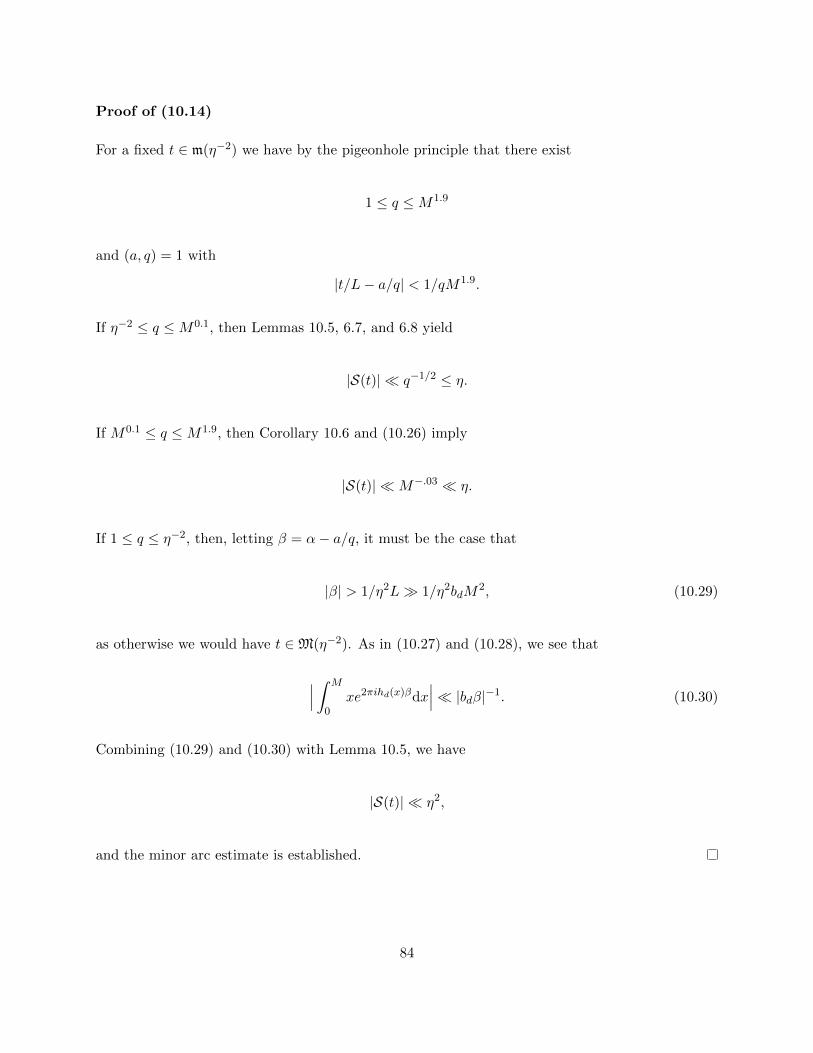
Proof of (10.14)
For a fixed t ∈ m(η−2) we have by the pigeonhole principle that there exist
1 ≤ q ≤M1.9
and (a, q) = 1 with
|t/L− a/q| < 1/qM1.9.
If η−2 ≤ q ≤M0.1, then Lemmas 10.5, 6.7, and 6.8 yield
|S(t)| � q−1/2 ≤ η.
If M0.1 ≤ q ≤M1.9, then Corollary 10.6 and (10.26) imply
|S(t)| �M−.03 � η.
If 1 ≤ q ≤ η−2, then, letting β = α− a/q, it must be the case that
|β| > 1/η2L� 1/η2bdM2, (10.29)
as otherwise we would have t ∈M(η−2). As in (10.27) and (10.28), we see that
∣∣∣ ∫ M
0xe2πihd(x)βdx
∣∣∣� |bdβ|−1. (10.30)
Combining (10.29) and (10.30) with Lemma 10.5, we have
|S(t)| � η2,
and the minor arc estimate is established.
84
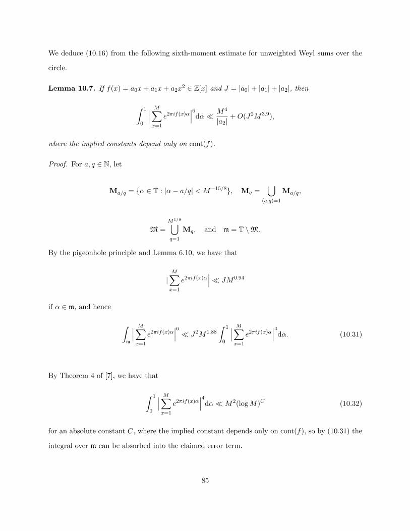
We deduce (10.16) from the following sixth-moment estimate for unweighted Weyl sums over the
circle.
Lemma 10.7. If f(x) = a0x+ a1x+ a2x2 ∈ Z[x] and J = |a0|+ |a1|+ |a2|, then
∫ 1
0
∣∣∣ M∑x=1
e2πif(x)α∣∣∣6dα� M4
|a2|+O(J2M3.9),
where the implied constants depend only on cont(f).
Proof. For a, q ∈ N, let
Ma/q = {α ∈ T : |α− a/q| < M−15/8}, Mq =⋃
(a,q)=1
Ma/q,
M =M1/8⋃q=1
Mq, and m = T \M.
By the pigeonhole principle and Lemma 6.10, we have that
|M∑x=1
e2πif(x)α∣∣∣� JM0.94
if α ∈ m, and hence
∫m
∣∣∣ M∑x=1
e2πif(x)α∣∣∣6 � J2M1.88
∫ 1
0
∣∣∣ M∑x=1
e2πif(x)α∣∣∣4dα. (10.31)
By Theorem 4 of [7], we have that
∫ 1
0
∣∣∣ M∑x=1
e2πif(x)α∣∣∣4dα�M2(logM)C (10.32)
for an absolute constant C, where the implied constant depends only on cont(f), so by (10.31) the
integral over m can be absorbed into the claimed error term.
85
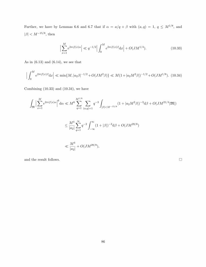
Further, we have by Lemmas 6.6 and 6.7 that if α = a/q + β with (a, q) = 1, q ≤ M1/8, and
|β| < M−15/8, then
∣∣∣ M∑x=1
e2πif(x)α∣∣∣� q−1/2
∣∣∣ ∫ M
0e2πif(x)βdx
∣∣∣+O(JM1/4). (10.33)
As in (6.13) and (6.14), we see that
∣∣∣ ∫ M
0e2πif(x)βdx
∣∣∣� min{M, |a2β|−1/2 +O(JM2β)} �M(1+ |a2M2β|)−1/2 +O(JM1/8). (10.34)
Combining (10.33) and (10.34), we have
∫M
∣∣∣ M∑x=1
e2πif(x)α∣∣∣6dα�M6
M1/8∑q=1
∑(a,q)=1
q−3
∫|β|<M−15/8
(1 + |a2M2β|)−3dβ +O(JM21/4|M|)
≤ M4
|a2|
∞∑q=1
q−2
∫ ∞−∞
(1 + |β|)−3dβ +O(JM29/8)
� M4
|a2|+O(JM29/8),
and the result follows.
86
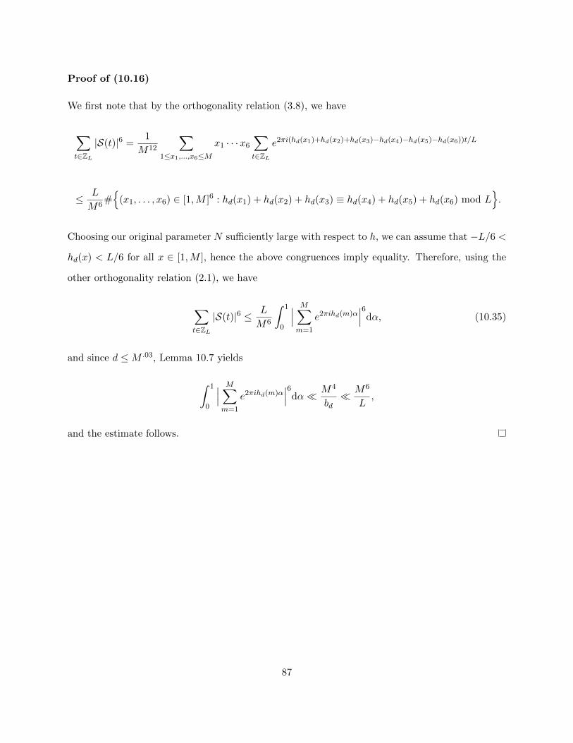
Proof of (10.16)
We first note that by the orthogonality relation (3.8), we have
∑t∈ZL
|S(t)|6 =1
M12
∑1≤x1,...,x6≤M
x1 · · ·x6
∑t∈ZL
e2πi(hd(x1)+hd(x2)+hd(x3)−hd(x4)−hd(x5)−hd(x6))t/L
≤ L
M6#{
(x1, . . . , x6) ∈ [1,M ]6 : hd(x1) + hd(x2) + hd(x3) ≡ hd(x4) + hd(x5) + hd(x6) mod L}.
Choosing our original parameter N sufficiently large with respect to h, we can assume that −L/6 <
hd(x) < L/6 for all x ∈ [1,M ], hence the above congruences imply equality. Therefore, using the
other orthogonality relation (2.1), we have
∑t∈ZL
|S(t)|6 ≤ L
M6
∫ 1
0
∣∣∣ M∑m=1
e2πihd(m)α∣∣∣6dα, (10.35)
and since d ≤M .03, Lemma 10.7 yields
∫ 1
0
∣∣∣ M∑m=1
e2πihd(m)α∣∣∣6dα� M4
bd� M6
L,
and the estimate follows.
87
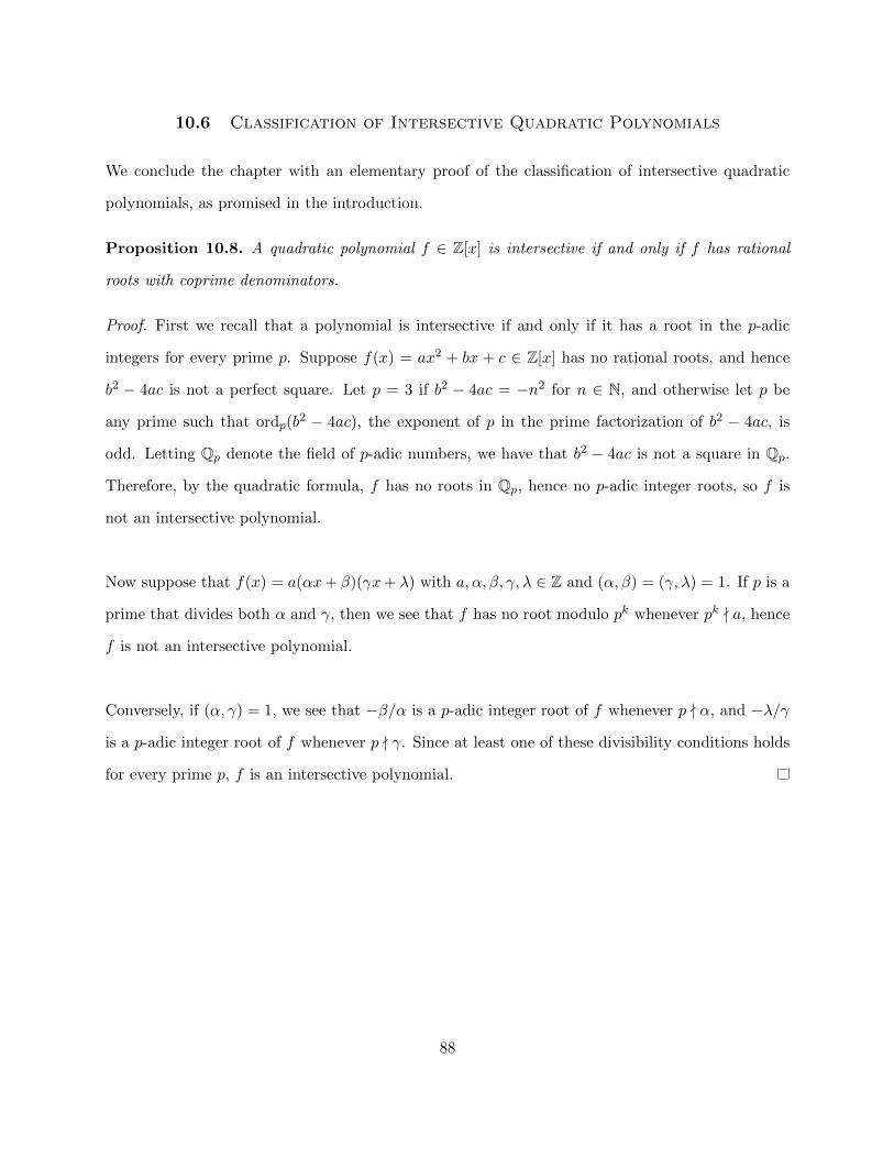
10.6 Classification of Intersective Quadratic Polynomials
We conclude the chapter with an elementary proof of the classification of intersective quadratic
polynomials, as promised in the introduction.
Proposition 10.8. A quadratic polynomial f ∈ Z[x] is intersective if and only if f has rational
roots with coprime denominators.
Proof. First we recall that a polynomial is intersective if and only if it has a root in the p-adic
integers for every prime p. Suppose f(x) = ax2 + bx + c ∈ Z[x] has no rational roots, and hence
b2 − 4ac is not a perfect square. Let p = 3 if b2 − 4ac = −n2 for n ∈ N, and otherwise let p be
any prime such that ordp(b2 − 4ac), the exponent of p in the prime factorization of b2 − 4ac, is
odd. Letting Qp denote the field of p-adic numbers, we have that b2 − 4ac is not a square in Qp.
Therefore, by the quadratic formula, f has no roots in Qp, hence no p-adic integer roots, so f is
not an intersective polynomial.
Now suppose that f(x) = a(αx+ β)(γx+ λ) with a, α, β, γ, λ ∈ Z and (α, β) = (γ, λ) = 1. If p is a
prime that divides both α and γ, then we see that f has no root modulo pk whenever pk - a, hence
f is not an intersective polynomial.
Conversely, if (α, γ) = 1, we see that −β/α is a p-adic integer root of f whenever p - α, and −λ/γ
is a p-adic integer root of f whenever p - γ. Since at least one of these divisibility conditions holds
for every prime p, f is an intersective polynomial.
88
11 Improved Bounds for
P-intersective Quadratic Polynomials
In this chapter we modify the method used to prove Theorem 10.1 and establish the analogous
result for P-intersective quadratic polynomials.
Theorem 11.1. Suppose h ∈ Z[x] is a P-intersective quadratic polynomial with positive leading
term. If A ⊆ [1, N ] and h(p) /∈ A−A for all primes p with h(p) > 0, then
|A|N� (logN)−µ log log log logN
for any µ < 1/2 log 3, where the implied constant depends only on h and µ.
11.1 Reduction of Theorem 11.1 to Two Lemmas
We fix a natural number N and a P-intersective quadratic polynomial h ∈ Z[x] with positive leading
term. We fix p-adic integer roots zp of h for each prime p with zp 6≡ 0 mod p, which determine
roots rd ∈ (−d, 0] of h modulo each d ∈ N satisfying (rd, d) = 1, and we let the function λ and the
auxiliary polynomials hd be as in Definition 6.2. We let Λd and Vd(h) be as defined in Section 7.1,
and we fix a set A ⊆ [1, N ] with |A| = δN and h(p) /∈ A−A for all p ∈ P with h(p) > 0, that is to
say (A−A) ∩ V1(h) = ∅. We also fix an arbitrary ε > 0, set Z = (logN)ε log log logN and γ = 2 + ε,
and we prove Theorem 11.1 with µ = (1− 22ε)/2 log(γ + 1).
Further, we set K = 220 and Q = ec√
logN as in Section 7.1, as well as the same q0 ≤ Q10K ,
ρ ∈ [1/2, 1), and Dirichlet character χ guaranteed by Lemma 5.2. In particular, we again have that
if c is sufficiently small and X ≥ N1/10, then
89
ψ(x, a, q) =x
φ(q)− χ(a)xρ
φ(q)ρ+O(XQ−1000K2
) (11.1)
for all x ≤ X, provided q0 | q, (a, q) = 1, and q ≤ (q0Q)10K . We deduce Theorem 11.1 from the
following two lemmas, analogous to Lemmas 10.2 and 10.3, respectively.
Lemma 11.2. If
δ ≥ e−(logN)ε/8 , (11.2)
then there exists B ⊆ [1, L] satisfying L ≥ N/QC , |B|/L = σ ≥ δ, and (B − B) ∩ Vd(h) = ∅ with
q0 | d and d/q0 ≤ Q. Further, B satisfies |B ∩ [1, L/2]| ≥ σL/3 and
maxq≤Z
∑t∈Mq(Z)
|B(t)|2 ≤ σ2(logN)−1/2+ε. (11.3)
Lemma 11.3. Suppose B ⊆ [1, L] is as in the conclusion of Lemma 11.2, let B1 = B ∩ [1, L/2],
and suppose σ ≥ Z−1/6. Given U, V,K ∈ N with max{U, V,K} ≤ Z1/6 and a set
P ⊆
t ∈V⋃q=1
Mq(K) ∪ {0} : |B1(t)| ≥ σ
U
satisfying
|P ∩Ma,q(K)| ≤ 1 whenever q ≤ V, (11.4)
there exist U ′, V ′,K ′ ∈ N with max{U ′, V ′,K ′} � (max{U, V,K})γ+1σ−5/2 and a set
P ′ ⊆
t ∈V ′⋃q=1
Mq(K′) ∪ {0} : |B1(t)| ≥ σ
U ′
(11.5)
satisfying
|P ′ ∩Ma,q(K′)| ≤ 1 whenever q ≤ V ′ (11.6)
and
|P ′|(U ′)2
≥ |P |U2
(logN)1/2−10ε. (11.7)
90
Proof of Theorem 11.1
In order to prove Theorem 11.1, we can assume that
δ ≥ (logN)− log log log logN .
Therefore, Lemma 10.2 produces a set B of density σ ≥ δ with the stipulated properties, and we set
P0 = {0}, U0 = 3, and V0 = K0 = 1. Lemma 11.3 then yields, for each n, a set Pn with parameters
Un, Vn,Kn such that
max{Un, Vn,Kn} ≤ (logN)(γ+1)n+1 log log log logN
and
1
σ≥ 1
σ2
∑t∈Pn
|B1(t)|2 ≥ |Pn|U2n
� (logN)n(1/2−10ε),
where the left-hand inequality comes from Plancherel’s Identity, as long as max{Un, Vn,Kn} ≤ Z1/6.
This holds with n = (1− ε)(log log log logN)/ log(γ + 1), as (γ + 1)n+1 ≤ (log log logN)1−ε/2, and
Theorem 10.1 follows.
11.2 The Outer Iteration II
Just like Lemma 10.2, we deduce Lemma 11.2 from a density increment lemma which follows
immediately from Lemma 9.2 and Proposition 7.2.
Lemma 11.4. Suppose B ⊆ [1, L] with |B| = σL and (B −B) ∩ Vd(h) = ∅. If L ≥ Z4 and
∑t∈Mq(Z)
|B(t)|2 ≥ σ2(logN)−1/2+ε, (11.8)
for some q ≤ Z, then there exists B′ ⊆ [1, L′] satisfying L′ � σL/Z4, (B′ −B′) ∩ Vqd(h) = ∅, and
|B′|/L′ ≥ σ(1 + (logN)−1/2+ε/8).
91
Proof of Lemma 11.2
Partitioning [1, N ], the pigeonhole principle guarantees the existence of an arithmetic progression
P = {x+ `λ(q0) : 1 ≤ ` ≤ N0} ⊆ [1, N ]
with N0 ≥ N/2λ(q0) and |A ∩ P | ≥ δN0. Defining A0 ⊆ [1, N0] by
A′ = {` ∈ [1, N0] : x+ `λ(q0) ∈ A},
we see that |A0| ≥ δN0 and (A − A) ∩ Vq0(h) = ∅. Lemma 11.4 then yields, for each k, a set
Ak ⊆ [1, Nk] with |Ak| = δkNk and (Ak −Ak) ∩ Vdk(h) = ∅ satisfying
Nk ≥ (cδ/Z4)kN/q20, δk ≥ δk−1(1 + (logN)−1/2+ε/8), q0 | dk, and dk/q0 ≤ Zk (11.9)
as long as Nk ≥ Z4 and either
maxq≤Z
∑t∈Mq(Z)
|Ak(t)|2 ≥ δ2k(logN)−1/2+ε (11.10)
or |Ak ∩ [1, Nk/2]| < δkNk/3, as the latter condition implies Ak has density at least 3δk/2 on the
interval (Nk/2, Nk]. We see that by (11.2) and (11.9), the density δk will exceed 1 after
16 log(δ−1)(logN)1/2−ε ≤ (logN)1/2−ε/2
steps, hence Nk < Z4 or (10.9) fails and |Ak ∩ [1, Nk/2]| ≥ δkNk/3 for some
k ≤ (logN)1/2−ε/2. (11.11)
However, we see that (11.2), (11.9), and (11.11) imply
Nk ≥ N(e−(logN)ε/4)(logN)1/2−ε/2q−20 ≥ N/QC ,
92
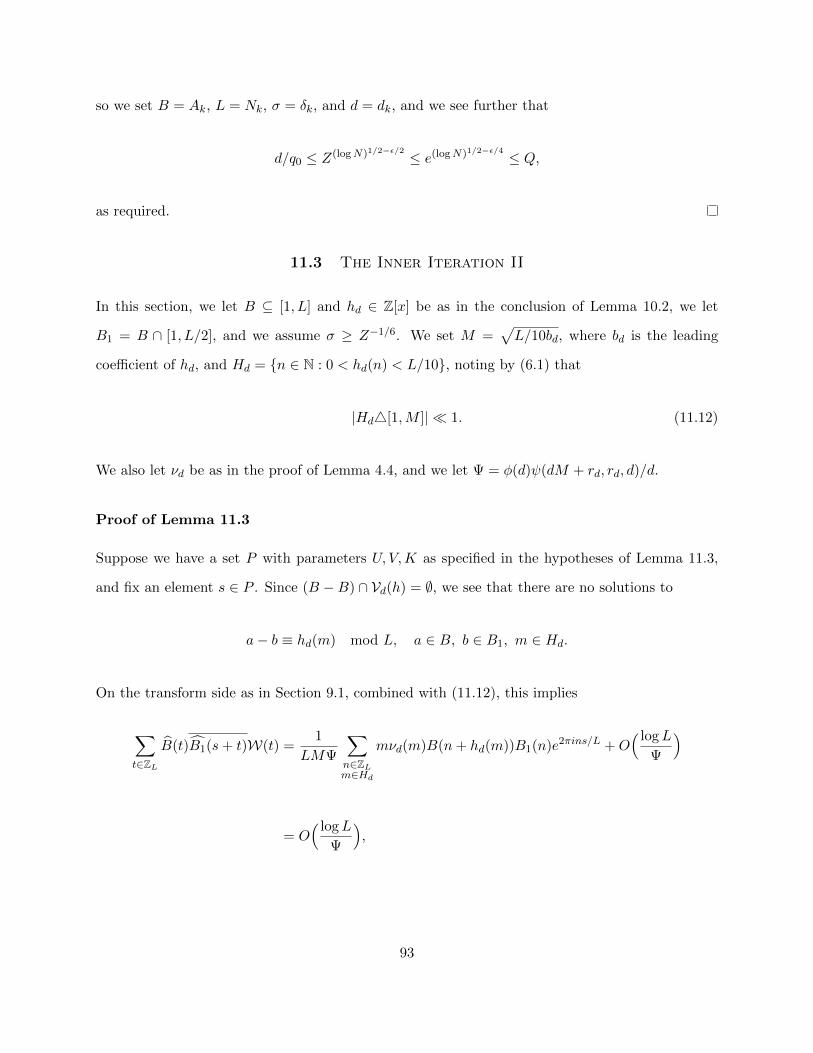
so we set B = Ak, L = Nk, σ = δk, and d = dk, and we see further that
d/q0 ≤ Z(logN)1/2−ε/2 ≤ e(logN)1/2−ε/4 ≤ Q,
as required.
11.3 The Inner Iteration II
In this section, we let B ⊆ [1, L] and hd ∈ Z[x] be as in the conclusion of Lemma 10.2, we let
B1 = B ∩ [1, L/2], and we assume σ ≥ Z−1/6. We set M =√L/10bd, where bd is the leading
coefficient of hd, and Hd = {n ∈ N : 0 < hd(n) < L/10}, noting by (6.1) that
|Hd4[1,M ]| � 1. (11.12)
We also let νd be as in the proof of Lemma 4.4, and we let Ψ = φ(d)ψ(dM + rd, rd, d)/d.
Proof of Lemma 11.3
Suppose we have a set P with parameters U, V,K as specified in the hypotheses of Lemma 11.3,
and fix an element s ∈ P . Since (B −B) ∩ Vd(h) = ∅, we see that there are no solutions to
a− b ≡ hd(m) mod L, a ∈ B, b ∈ B1, m ∈ Hd.
On the transform side as in Section 9.1, combined with (11.12), this implies
∑t∈ZL
B(t)B1(s+ t)W(t) =1
LMΨ
∑n∈ZLm∈Hd
mνd(m)B(n+ hd(m))B1(n)e2πins/L +O( logL
Ψ
)
= O( logL
Ψ
),
93
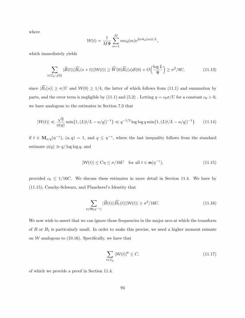
where
W(t) =1
MΨ
M∑m=1
mνd(m)e2πihd(m)t/L,
which immediately yields
∑t∈ZL\{0}
|B(t)||B1(s+ t)||W(t)| ≥ W (0)B1(s)S(0) +O( logL
Ψ
)≥ σ2/8U, (11.13)
since |B1(s)| ≥ σ/U and W(0) ≥ 1/4, the latter of which follows from (11.1) and summation by
parts, and the error term is negligible by (11.1) and (5.2) . Letting η = c0σ/U for a constant c0 > 0,
we have analogous to the estimates in Section 7.3 that
|W(t)| �√q
φ(q)min{1, (L|t/L− a/q|)−1} � q−1/2 log log qmin{1, (L|t/L− a/q|)−1} (11.14)
if t ∈ Ma/q(η−γ), (a, q) = 1, and q ≤ η−γ , where the last inequality follows from the standard
estimate φ(q)� q/ log log q, and
|W(t)| ≤ Cη ≤ σ/16U for all t ∈ m(η−γ), (11.15)
provided c0 ≤ 1/16C. We discuss these estimates in more detail in Section 11.4. We have by
(11.15), Cauchy-Schwarz, and Plancherel’s Identity that
∑t∈M(η−γ)
|B(t)||B1(t)||W(t)| ≥ σ2/16U. (11.16)
We now wish to assert that we can ignore those frequencies in the major arcs at which the transform
of B or B1 is particularly small. In order to make this precise, we need a higher moment esimate
on W analogous to (10.16). Specifically, we have that
∑t∈ZL
|W(t)|6 ≤ C, (11.17)
of which we provide a proof in Section 11.4.
94
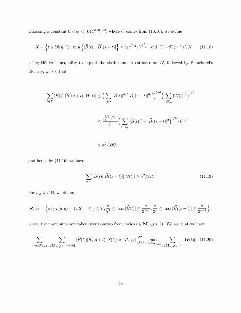
Choosing a constant 0 < c1 < (64C1/6)−3, where C comes from (10.16), we define
X ={t ∈M(η−γ) : min
{|B(t)|, |B1(s+ t)|
}≤ c1σ
7/2/U3}
and Y = M(η−γ) \X. (11.18)
Using Holder’s Inequality to exploit the sixth moment estimate on W, followed by Plancherel’s
Identity, we see that
∑t∈X|B(t)||B1(s+ t)||W(t)| ≤
(∑t∈X|B(t)|6/5|B1(s+ t)|6/5
)5/6( ∑t∈ZL
|W(t)|6)1/6
≤ c1/31 σ7/6
U
( ∑t∈ZL
|B(t)|2 + |B1(s+ t)|2)5/6
· C1/6
≤ σ2/32U,
and hence by (11.16) we have
∑t∈Y|B(t)||B1(s+ t)||W(t)| ≥ σ2/32U. (11.19)
For i, j, k ∈ N, we define
Ri,j,k ={a/q : (a, q) = 1, 2i−1 ≤ q ≤ 2i,
σ
2j≤ max |B(t)| ≤ σ
2j−1,σ
2k≤ max |B1(s+ t)| ≤ σ
2k−1
},
where the maximums are taken over nonzero frequencies t ∈Ma/q(η−γ). We see that we have
∑a/q∈Ri,j,k
∑t∈Ma/q(η
−γ)\{0}
|B(t)||B1(s+ t)||S(t)| � |Ri,j,k|σ2
2j2kmax
a/q∈Ri,j,k
∑t∈Ma/q(η
−γ)
|W(t)|. (11.20)
95
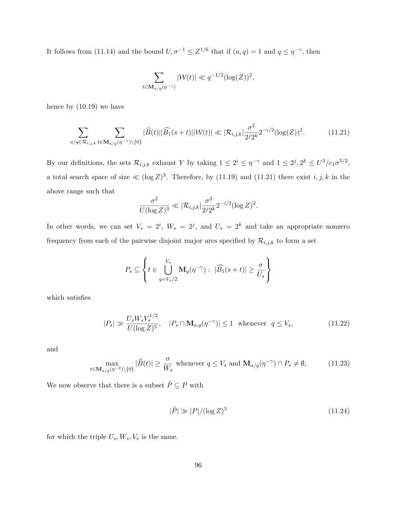
It follows from (11.14) and the bound U, σ−1 ≤ Z1/6 that if (a, q) = 1 and q ≤ η−γ , then
∑t∈Ma/q(η
−γ)
|W(t)| � q−1/2(log(Z))2,
hence by (10.19) we have
∑a/q∈Ri,j,k
∑t∈Ma/q(η
−γ)\{0}
|B(t)||B1(s+ t)||W(t)| � |Ri,j,k|σ2
2j2k2−i/2(log(Z))2. (11.21)
By our definitions, the sets Ri,j,k exhaust Y by taking 1 ≤ 2i ≤ η−γ and 1 ≤ 2j , 2k ≤ U3/c1σ5/2,
a total search space of size � (logZ)3. Therefore, by (11.19) and (11.21) there exist i, j, k in the
above range such that
σ2
U(logZ)3� |Ri,j,k|
σ2
2j2k2−i/2(logZ)2.
In other words, we can set Vs = 2i, Ws = 2j , and Us = 2k and take an appropriate nonzero
frequency from each of the pairwise disjoint major arcs specified by Ri,j,k to form a set
Ps ⊆
t ∈Vs⋃
q=Vs/2
Mq(η−γ) : |B1(s+ t)| ≥ σ
Us
which satisfies
|Ps| �UsWsV
1/2s
U(logZ)5, |Ps ∩Ma,q(η
−γ)| ≤ 1 whenever q ≤ Vs, (11.22)
and
maxt∈Ma/q(η
−2)\{0}|B(t)| ≥ σ
Wswhenever q ≤ Vs and Ma/q(η
−γ) ∩ Ps 6= ∅, (11.23)
We now observe that there is a subset P ⊆ P with
|P | � |P |/(logZ)3 (11.24)
for which the triple Us,Ws, Vs is the same.
96
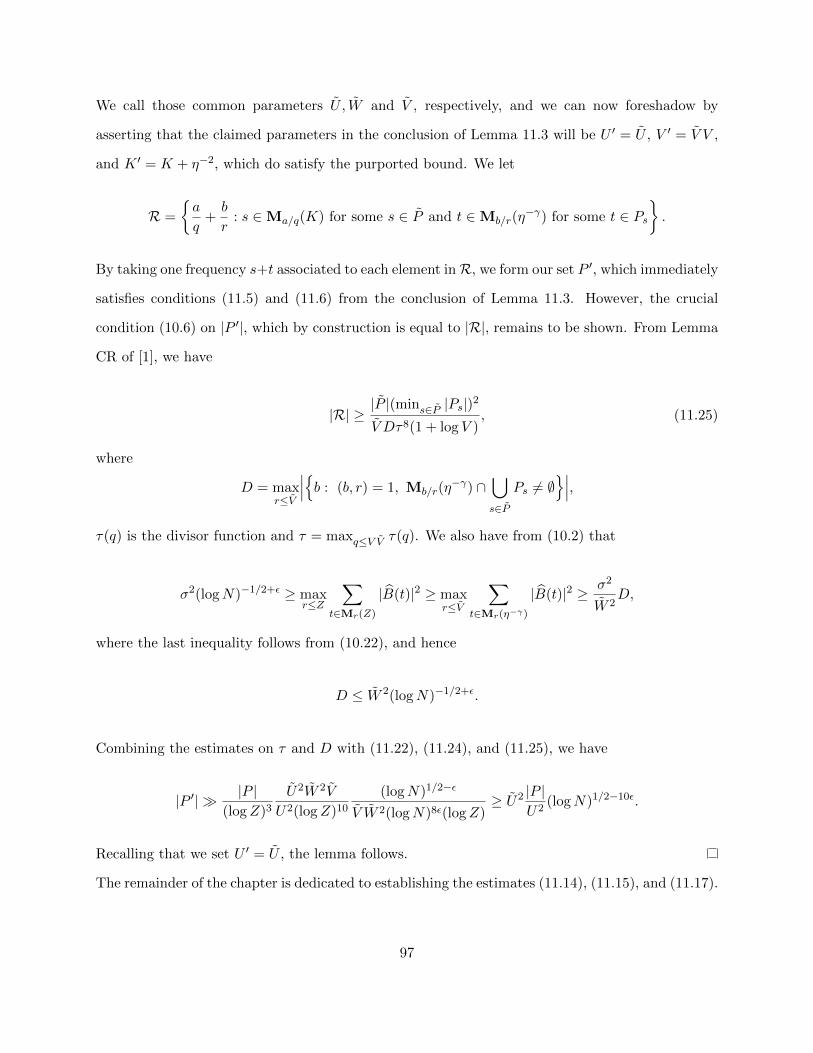
We call those common parameters U , W and V , respectively, and we can now foreshadow by
asserting that the claimed parameters in the conclusion of Lemma 11.3 will be U ′ = U , V ′ = V V ,
and K ′ = K + η−2, which do satisfy the purported bound. We let
R =
{a
q+b
r: s ∈Ma/q(K) for some s ∈ P and t ∈Mb/r(η
−γ) for some t ∈ Ps}.
By taking one frequency s+t associated to each element inR, we form our set P ′, which immediately
satisfies conditions (11.5) and (11.6) from the conclusion of Lemma 11.3. However, the crucial
condition (10.6) on |P ′|, which by construction is equal to |R|, remains to be shown. From Lemma
CR of [1], we have
|R| ≥|P |(mins∈P |Ps|)
2
V Dτ8(1 + log V ), (11.25)
where
D = maxr≤V
∣∣∣{b : (b, r) = 1, Mb/r(η−γ) ∩
⋃s∈P
Ps 6= ∅}∣∣∣,
τ(q) is the divisor function and τ = maxq≤V V τ(q). We also have from (10.2) that
σ2(logN)−1/2+ε ≥ maxr≤Z
∑t∈Mr(Z)
|B(t)|2 ≥ maxr≤V
∑t∈Mr(η−γ)
|B(t)|2 ≥ σ2
W 2D,
where the last inequality follows from (10.22), and hence
D ≤ W 2(logN)−1/2+ε.
Combining the estimates on τ and D with (11.22), (11.24), and (11.25), we have
|P ′| � |P |(logZ)3
U2W 2V
U2(logZ)10
(logN)1/2−ε
V W 2(logN)8ε(logZ)≥ U2 |P |
U2(logN)1/2−10ε.
Recalling that we set U ′ = U , the lemma follows.
The remainder of the chapter is dedicated to establishing the estimates (11.14), (11.15), and (11.17).
97
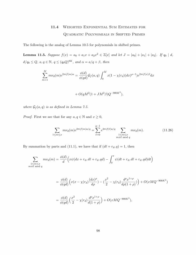
11.4 Weighted Exponential Sum Estimates for
Quadratic Polynomials in Shifted Primes
The following is the analog of Lemma 10.5 for polynomials in shifted primes.
Lemma 11.5. Suppose f(x) = a0 + a1x + a2x2 ∈ Z[x] and let J = |a0| + |a1| + |a2|. If q0 | d,
d/q0 ≤ Q, a, q ∈ N, q ≤ (q0Q)8K , and α = a/q + β, then
M∑m=1
mνd(m)e2πif(m)α =φ(d)
φ(qd)Gf (a, q)
∫ M
0x(1− χ(rd)(dx)ρ−1)e2πif(x)βdx
+O(qM2(1 + JM2β)Q−900K2),
where Gf (a, q) is as defined in Lemma 7.5.
Proof. First we see that for any a, q ∈ N and x ≥ 0,
∑1≤m≤x
mνd(m)e2πif(m)a/q =
q−1∑`=0
e2πif(`)a/q∑
1≤m≤xm≡` mod q
mνd(m). (11.26)
By summation by parts and (11.1), we have that if (d`+ rd, q) = 1, then
∑1≤m≤x
m≡` mod q
mνd(m) =φ(d)
d
(xψ(dx+ rd, d`+ rd, qd)−
∫ x
0ψ(dt+ rd, d`+ rd, qd)dt
)
=φ(d)
φ(qd)
(x(x− χ(rd)
(dx)ρ
dρ)− (
x2
2− χ(rd)
dρx1+ρ
dρ(1 + ρ)))
+O(xMQ−900K2)
=φ(d)
φ(qd)
(x2
2− χ(rd)
dρx1+ρ
d(1 + ρ)
)+O(xMQ−900K2
),
98
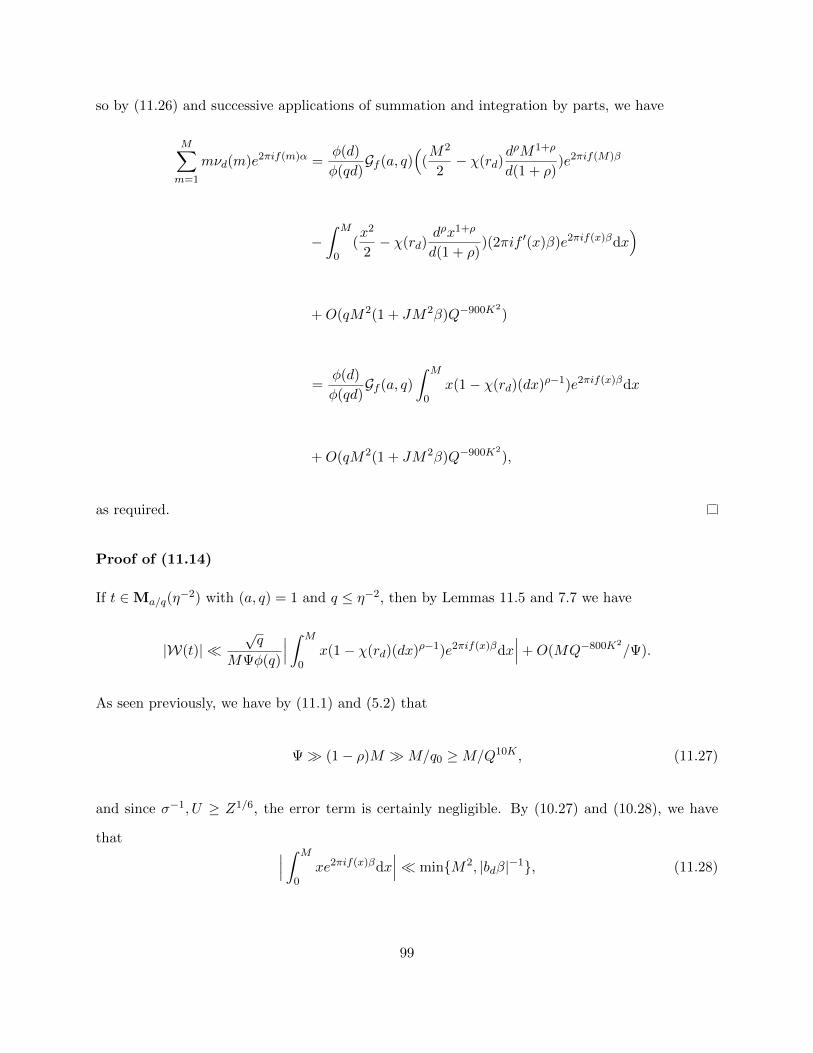
so by (11.26) and successive applications of summation and integration by parts, we have
M∑m=1
mνd(m)e2πif(m)α =φ(d)
φ(qd)Gf (a, q)
((M2
2− χ(rd)
dρM1+ρ
d(1 + ρ))e2πif(M)β
−∫ M
0(x2
2− χ(rd)
dρx1+ρ
d(1 + ρ))(2πif ′(x)β)e2πif(x)βdx
)
+O(qM2(1 + JM2β)Q−900K2)
=φ(d)
φ(qd)Gf (a, q)
∫ M
0x(1− χ(rd)(dx)ρ−1)e2πif(x)βdx
+O(qM2(1 + JM2β)Q−900K2),
as required.
Proof of (11.14)
If t ∈Ma/q(η−2) with (a, q) = 1 and q ≤ η−2, then by Lemmas 11.5 and 7.7 we have
|W(t)| �√q
MΨφ(q)
∣∣∣ ∫ M
0x(1− χ(rd)(dx)ρ−1)e2πif(x)βdx
∣∣∣+O(MQ−800K2/Ψ).
As seen previously, we have by (11.1) and (5.2) that
Ψ� (1− ρ)M �M/q0 ≥M/Q10K , (11.27)
and since σ−1, U ≥ Z1/6, the error term is certainly negligible. By (10.27) and (10.28), we have
that ∣∣∣ ∫ M
0xe2πif(x)βdx
∣∣∣� min{M2, |bdβ|−1}, (11.28)
99
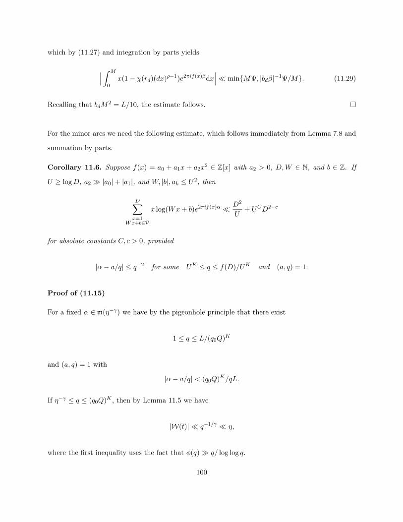
which by (11.27) and integration by parts yields
∣∣∣ ∫ M
0x(1− χ(rd)(dx)ρ−1)e2πif(x)βdx
∣∣∣� min{MΨ, |bdβ|−1Ψ/M}. (11.29)
Recalling that bdM2 = L/10, the estimate follows.
For the minor arcs we need the following estimate, which follows immediately from Lemma 7.8 and
summation by parts.
Corollary 11.6. Suppose f(x) = a0 + a1x + a2x2 ∈ Z[x] with a2 > 0, D,W ∈ N, and b ∈ Z. If
U ≥ logD, a2 � |a0|+ |a1|, and W, |b|, ak ≤ U2, then
D∑x=1
Wx+b∈P
x log(Wx+ b)e2πif(x)α � D2
U+ UCD2−c
for absolute constants C, c > 0, provided
|α− a/q| ≤ q−2 for some UK ≤ q ≤ f(D)/UK and (a, q) = 1.
Proof of (11.15)
For a fixed α ∈ m(η−γ) we have by the pigeonhole principle that there exist
1 ≤ q ≤ L/(q0Q)K
and (a, q) = 1 with
|α− a/q| < (q0Q)K/qL.
If η−γ ≤ q ≤ (q0Q)K , then by Lemma 11.5 we have
|W(t)| � q−1/γ � η,
where the first inequality uses the fact that φ(q)� q/ log log q.
100

If (q0Q)K ≤ q ≤ L/(q0Q)K , then by Corollary 11.6, (11.27), and the bounds σ−1, U ≤ Z1/6, we
have
|W(t)| �M/Ψq0Q ≤ η.
If 1 ≤ q ≤ η−γ , then letting β = α− a/q, we must have
|β| > 1/ηγL� 1/ηγbdM2. (11.30)
Combining (11.30) with Lemma 11.5 and (11.29) yields
|W(t)| � ηγ ,
and the minor arc estimate is established.
Proof of (11.17)
Analogous to the proof of (10.16), we have
∑t∈ZL
|W(t)|6 ≤ L
Ψ6
∫ 1
0
∣∣∣ M∑m=1
νd(m)e2πihd(m)α∣∣∣6dα. (11.31)
Reverting to the definitions of major and minor arcs on the circle from Chapter 2.3, we have by
the pigeonhole principle and Lemma 7.8 that
|M∑m=1
νd(m)e2πihd(m)α∣∣∣�M/(q0Q)8 (11.32)
for all α ∈ m((q0Q)8K).
101
Combined with (10.32), (11.27), and the bound bd � d ≤ q0Q, (11.32) yields
∫m((q0Q)8K)
∣∣∣ M∑m=1
νd(m)e2πihd(m)α∣∣∣6dα ≤ M2(logM)6
(q0Q)8
∫ 1
0
∣∣∣ M∑m=1
e2πihd(m)α∣∣∣4dα
� M4(logM)C
(q0Q)8� Ψ6
(q0Q)3Ψ2� Ψ6
L.
Further, we have by Lemma 7.5, Corollary 7.7, and integration by parts that if α = a/q + β,
(a, q) = 1, q ≤ (q0Q)8K , and |β| < L/(q0Q)8K , then
∣∣∣ M∑m=1
νd(m)e2πihd(m)α∣∣∣� q−1/γ
∣∣∣ ∫ M
0(1− χ(rd)(dx)ρ−1)e2πihd(x)βdx
∣∣∣+O(MQ−500K2)
� q−1/γ min{Ψ, |bdβ|−1/2Ψ/M}
� q−1/γΨ(1 + |bdM2β|)−1/2
Finally, we have
∫M((qoQ)8K)
∣∣∣ M∑m=1
νd(m)e2πihd(m)α∣∣∣6 � Ψ6
(q0Q)8K∑q=1
∑(a,q)=1
q−5/2
∫|β|<(q0Q)8K/L
(1 + |bdM2β|)−3dβ
� Ψ6
bdM2
∞∑q=1
q−3/2
∫ ∞∞
(1 + |β|)−3dβ
� Ψ6
L,
and by (11.31) the estimate follows.
102
Bibliography
[1] A. Balog, J. Pelikan, J. Pintz, E. Szemeredi, Difference Sets Without k-th Powers,
Acta. Math. Hungar. 65 (2) (1994), pp. 165-187.
[2] D. Berend, Y. Bilu, Polynomials with roots modulo every integer, Proc. Amer. Math. Soc.
124 (1996), pp. 1663-1671.
[3] J. R. Chen, On Professor Hua’s estimate of exponential sums, Sci. Sinica 20 (1997), pp.
711-719.
[4] H. Furstenberg, Ergodic behavior of diagonal measures and a theorem of Szemeredi on
arithmetic progressions, J. d’Analyse Math, 71 (1977), 204-256.
[5] B. Green, On arithmetic structures in dense sets of integers, Duke Math. Jour. 114 (2002),
(2), pp. 215-238
[6] M. Hamel, N. Lyall, A. Rice, Improved bounds on Sarkozy’s theorem for quadratic poly-
nomials, to appear in Int. Math. Res. Not., arXiv:1111.5786v4.
[7] L. K. Hua, Additive theory of prime numbers , American Mathematical Society, Providence,
RI 1965.
[8] T. Kamae, M. Mendes France, van der Corput’s difference theorem, Israel J. Math. 31,
no. 3-4, (1978), pp. 335-342.
[9] H.-Z. Li, H. Pan, Difference sets and polynomials of prime variables, Acta. Arith. 138, no. 1
(2009), pp. 25-52.
[10] J. Lucier, Difference sets and shifted primes, Acta. Math. Hungar. 120 (2008), pp.79-102.
103
[11] J. Lucier, Intersective Sets Given by a Polynomial, Acta Arith. 123 (2006), pp. 57-95.
[12] N. Lyall, A new proof of Sarkozy’s Theorem, to appear in Proc. Amer. Math. Soc.,
arXiv:1107.0243v3.
[13] N. Lyall, A. Magyar, Polynomial configurations in difference sets, J. Number Theory 129
(2009), pp. 439-450.
[14] N. Lyall, A. Magyar, Simultaneous polynomial recurrence, Bull. Lond. Math. Soc. 43 (2011),
no. 4, pp. 765-785.
[15] H. L. Montgomery Ten lectures on the interface between analytic number theory and har-
monic analysis, CBMS Regional Conference Series in Mathematics, 84.
[16] H. L. Montgomery, R. C. Vaughan, Multiplicative Number Theory I. Classical Theory,
Cambridge Studies in Advanced Mathematics 97, 2007.
[17] V. I. Nechaev, An estimate of the complete rational trigonmetric sum, Mat. Zametki 17
(1975), pp. 839-849 (in Russian); English translation: Math. Notes 17 (1975), pp. 504-511.
[18] J. Pintz, W. L. Steiger, E. Szemeredi, On sets of natural numbers whose difference set
contains no squares, J. London Math. Soc. 37 (1988), pp. 219-231.
[19] A. Rice, Sarkozy’s theorem for P-intersective polynomials, to appear in Acta Arithmetica,
arXiv:1111.6559v3.
[20] K. F. Roth, On certain sets of integers, J. London Math. Soc. 28 (1953), pp. 104-109.
[21] I. Ruzsa, T. Sanders, Difference sets and the primes, Acta. Arith. 131, no. 3 (2008), pp.
281-201.
[22] A. Sarkozy, On difference sets of sequences of integers I, Acta. Math. Hungar. 31(1-2) (1978),
pp. 125-149.
[23] A. Sarkozy, On difference sets of sequences of integers III, Acta. Math. Hungar. 31(3-4)
(1978), pp. 355-386.
104
[24] S. Slijepcevic, A polynomial Sarkozy-Furstenberg theorem with upper bounds, Acta Math.
Hungar. 98 (2003), pp. 275-280
[25] R. C. Vaughan, The Hardy-Littlewood method, Cambridge University Press, Second Edition,
1997.
[26] M. Wierdl, Ph. D. Thesis, Ohio State University, 1989.
105