CSE 591 Randomized and ApproximationAlgorithms

Charlie Colbourn

School of Computing, Informatics, and Decision Systems EngineeringArizona State University

ASU, Fall 2010

Logistics

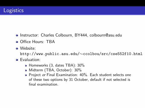
Instructor: Charles Colbourn, BY444, colbourn@asu.edu

Office Hours: TBA

Website:http://www.public.asu.edu/∼ccolbou/src/cse552f10.htmlEvaluation:

Homeworks (3, dates TBA): 30%Midterm (TBA, October): 30%Project or Final Examination: 40%. Each student selects oneof these two options by 31 October, default if not selected isfinal examination.

Randomization

Leaving decisions to chance.

Randomized algorithm: allowed to invoke a random event and usethe outcome to determine the next step.

Basic random events:

1 Basic: generate a random bit

2 Complex: generate a random number (int/float)

3 Complex: generate a random object of some general type

Uses of randomization

Randomization may

make complicated algorithms simpler

make inefficient computations efficient (quicksort, mincut)

make possible things we don’t know how to dodeterministically (primality testing in P, matching in parallel)

make possible things that are provably impossible to dodeterministically (volume computation, distributed protocols)

Example: quicksort

Input: set S of n numbers.Output: the elements of S sorted in increasing order.

1 Choose y ∈ S uniformly at random.

2 S1 = x ∈ S | x < y, S2 = x ∈ S | x > y.3 Recursively sort S1 and S2.

4 Output sorted S1, followed by y , followed by sorted S2.

1 Compare: Deterministic worst-case: O(n2) – element chosenis always the smallest remaining.

2 Average-case analysis: still deterministic, but average overdistribution of inputs. Depends on distribution.

Randomized quicksort analysis

Let s1 ≤ s2 ≤ . . . ≤ sn be the set S in order.Let

Xij =

1 si is compared to sj

0 si is not compared to sj

Number of comparisons made is Tn =∑n

i=1

∑j>i Xij .

Digression: discrete probability (1)

Sample space: set Ω of all possible outcomes (quicksort: the set ofall possible runs of the algorithm on input S)Events: subsets of Ω (example: let x be an element of S . The setAx of all possible runs where the first element selected is x)Probability of an event (Pr[Ax ] = 1/n).Random variable: mapping from Ω to real numbers (Xij).Expectation of a random variable: its “average value”,

E[X ] =∑ω∈Ω

Pr[ω] · X (ω)

(E[Xij ] = Pr[Xij = 1] · 1 + Pr[Xij = 0] · 0 = Pr[Xij = 1]).

Digression: discrete probability (2)

Expectation is linear: for random variables X and Y , numbers a, b,

E[aX + bY ] = aE[X ] + bE[Y ].

Example: in randomized quicksort,

E[Tn] = E[n∑

i=1

n∑j=i+1

Xij ]

=n∑

i=1

n∑j=i+1

E[Xij ]

=n∑

i=1

n∑j=i+1

Pr[Xij = 1].

Randomized quicksort analysis

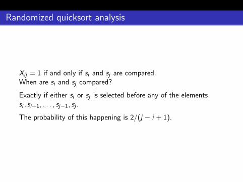
Xij = 1 if and only if si and sj are compared.When are si and sj compared?

Exactly if either si or sj is selected before any of the elementssi , si+1, . . . , sj−1, sj .

The probability of this happening is 2/(j − i + 1).

Randomized quicksort analysis

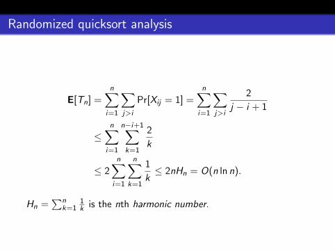
E[Tn] =n∑

i=1

∑j>i

Pr[Xij = 1] =n∑

i=1

∑j>i

2

j − i + 1

≤n∑

i=1

n−i+1∑k=1

2

k

≤ 2n∑

i=1

n∑k=1

1

k≤ 2nHn = O(n ln n).

Hn =∑n

k=11k is the nth harmonic number.

Cuts in graphs

A cut in G : a set of edges that disconnects the graph.For a set C ⊆ V , let C = V \ C . Then (C ,C ) defines a cut. Wewrite

(C ,C ) = uv ∈ E | u ∈ C , v ∈ C.

Minimum cut problem

Input: (multi)graph G = (V ,E ).Output: a cut of minimum cardinality in G .

Polynomially solvable, O(n3) time (but not simple). Solve usingnetwork flows.

Simple randomized algorithm for mincut

1 Pick an edge e uniformly at random.

2 Contract e.

3 Repeat until there are only two vertices left.

Claim: Contractions do not decrease the minimum cut value.

Randomized mincut analysis (1)

Let k be the minimum cut cardinality. Let C be a minimum cut.

G has at least kn/2 edges.

For i = 1, . . . , n − 2, let Ai be the event that no edge of C wascontracted in the i-th step.

If all of the events A1, . . .An−2 happen, then the algorithm findsthe minimum cut C .

Randomized mincut analysis (2)

Pr[A1] ≥ 1− 2

n=

n − 2

n.

If A1 happens, then before the second step of the algorithm thereare at least k(n − 1)/2 edges in the graph.

Pr[A2 | A1] ≥ 1− 2

n − 1=

n − 3

n − 1.

In general, if A1, . . . ,Ai−1 happen, then before the i-th step thereare at least k(n − i + 1)/2 edges in the graph and so

Pr[Ai | A1,A2, . . .Ai−1] ≥ 1− 2

n − i + 1=

n − i − 1

n − i + 1.

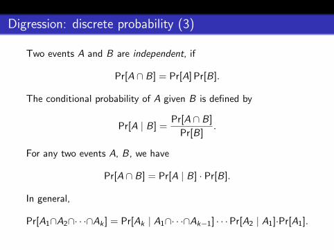
Digression: discrete probability (3)

Two events A and B are independent, if

Pr[A ∩ B] = Pr[A] Pr[B].

The conditional probability of A given B is defined by

Pr[A | B] =Pr[A ∩ B]

Pr[B].

For any two events A, B, we have

Pr[A ∩ B] = Pr[A | B] · Pr[B].

In general,

Pr[A1∩A2∩· · ·∩Ak ] = Pr[Ak | A1∩· · ·∩Ak−1] · · ·Pr[A2 | A1]·Pr[A1].

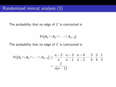
Randomized mincut analysis (3)

The probability that no edge of C is contracted is

Pr[A1 ∩ A2 ∩ · · · ∩ An−2]

The probability that no edge of C is contracted is

Pr[A1 ∩ A2 ∩ · · · ∩ An−2] ≥ n − 2

n· n − 3

n − 1· n − 4

n − 2· · · 3

5· 2

4· 1

3

=2

n(n − 1).

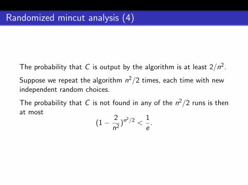
Randomized mincut analysis (4)

The probability that C is output by the algorithm is at least 2/n2.

Suppose we repeat the algorithm n2/2 times, each time with newindependent random choices.

The probability that C is not found in any of the n2/2 runs is thenat most

(1− 2

n2)n2/2 <

1

e.

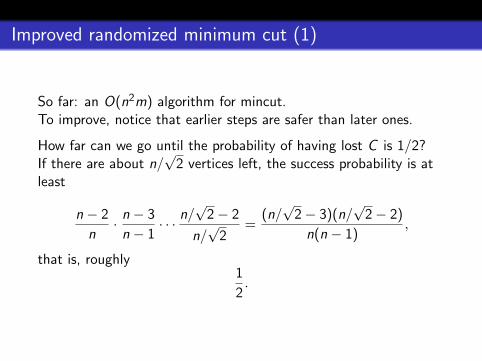
Improved randomized minimum cut (1)

So far: an O(n2m) algorithm for mincut.To improve, notice that earlier steps are safer than later ones.

How far can we go until the probability of having lost C is 1/2?If there are about n/

√2 vertices left, the success probability is at

least

n − 2

n· n − 3

n − 1· · · n/

√2− 2

n/√

2=

(n/√

2− 3)(n/√

2− 2)

n(n − 1),

that is, roughly1

2.

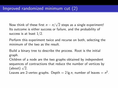
Improved randomized minimum cut (2)

Now think of these first n − n/√

2 steps as a single experiment!Its outcome is either success or failure, and the probability ofsuccess is at least 1/2.

Perform this experiment twice and recurse on both, selecting theminimum of the two as the result.

Build a binary tree to describe the process. Root is the initialgraph.Children of a node are the two graphs obtained by independentsequences of contractions that reduce the number of vertices by(about)

√2.

Leaves are 2-vertex graphs. Depth = 2 lg n, number of leaves = n2.

Improved randomized minimum cut (3)

If Pd is the probability a path survives in a tree of depth d , then

Pd =1

2Pd−1 +

1

4(1− (1− Pd−1)2)

=1

2Pd−1 +

1

4(2Pd−1 − (Pd−1)2)

= Pd−1 −1

4(Pd−1)2.

Now if Pd−1 >1

d−1 , then

Pd >1

d − 1− 1

4(d − 1)2>

1

d − 1− 1

d(d − 1)=

1

d.

So the probability a path survives is Ω( 1log n ).

To make this a constant, repeat independently log n times.

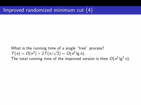
Improved randomized minimum cut (4)

What is the running time of a single “tree” process?T (n) = O(n2) + 2T (n/

√2) = O(n2 lg n).

The total running time of the improved version is then O(n2 lg2 n).

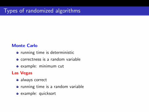
Types of randomized algorithms

Monte Carlo

running time is deterministic

correctness is a random variable

example: minimum cut

Las Vegas

always correct

running time is a random variable

example: quicksort