Cutting planes for improved global logic-based outer approximation

for the synthesis of process networks.

Francisco Trespalacios, Ignacio E. Grossmann∗

Department of Chemical Engineering, Carnegie Mellon University

5000 Forbes Avenue, Pittsburgh, PA 15213, USA

∗ Author to whom correspondence should be addressed: grossmann@cmu.edu

Abstract

In this work, we present an improved global logic-based outer approximation method (GLBOA) for

the solution of nonconvex generalized disjunctive programs (GDP). The GLBOA allows the solution of

nonconvex GDP models, and is particularly useful for optimizing the synthesis of process networks. Two

enhancements to the basic GLBOA are presented. The first enhancement seeks to obtain feasible solutions

faster by dividing the basic algorithm into two stages. The second enhancement seeks to tighten the lower

bound of the algorithm by the use of cutting planes. The proposed method for obtaining cutting planes, the

main contribution of this work, is a separation problem based in the convex hull of the feasible region of a

subset of the constraints. Results show that the enhancements improve the performance of the algorithm,

and that the algorithm is better in finding better feasible solutions than general purpose global solvers in the

tested problems.

1 Introduction

The synthesis of process networks is an area of active research in Process Systems Engineering (PSE). The ob-

jective is to synthesize the optimal process flowsheet contained in a process superstructure[1], which contains

alternative units (with their corresponding models) and interconnections. The synthesis process networks can

be modeled as a mixed-integer nonlinear problem (MINLP) [2]. In the MINLP approach, the selection of

units and interconnections are modeled using binary variables. The process unknowns (flow, concentration,

temperature, etc.) are modeled using continuous variables. Alternative superstructure representations of

processes have also been proposed[3–6].

The synthesis of process networks yields MINLP models that can be highly nonconvex. In particular,

the nonconvexities arise in two forms. The first form involves the modelling of each individual process unit.

1

This models can range from linear input/output equations to large differential algebraic models. The second

form of noconvexities arise in the modeling of flow and properties that result when mixing streams, in the

simplest case as bilinear terms. It is important to note that when the units and interconnections are fixed in

a superstructure, the resulting problem is a nonlinear program (NLP). This NLP, not only is continuous, but

does not include nonconvexities related to the units or interconnections that were not selected. Because of

these two reasons, it is common that the resulting NLP after fixing the discrete decisions is much simpler to

solve than the full problem, provided that the constraints of the non-selected units and interconnections are

removed from the NLP model. This property is not general for MINLPs, but very common in the synthesis

process networks. General methods for solving MINLPs to global optimality do not take advantage of this

particular property.

The most common deterministic method for solving nonconvex MINLP problems is the spatial branch

and bound algorithm[7]. This algorithm is used by several general purpose MINLP global solvers, such as:

αBB[8], ANTIGONE[9], BARON[10, 11], Couenne[12], LINDO[13], and SCIP[14]. We refer the reader to

the work by Bussieck and Vigerske[15] for details of the different MINLP solvers. In addition to the spatial

branch and bound, Kesavan et al.[16] present an outer-approximation method for global optimization. This

method builds on the traditional outer-approximation method for convex optimization[17, 18].

Other methods have been developed to exploit the simplification of problems when discrete decisions

are fixed, typically in the form of logic-based Benders decomposition[19] (a generalization of the Benders

decomposition[20] and Generalized Benders decomposition[21]). In particular for nonconvex MINLP, Li et

al.[22] present a nonconvex generalized Benders decomposition method for stochastic MINLPs.

An alternative representation of MINLP is Generalized Disjunctive Programming (GDP)[23]. GDP mod-

els represent problems through the use of Boolean variables, algebraic equations and logic propositions[24].

Synthesis of process networks is one of the areas where GDP has been most successful. Raman and Gross-

mann[25] propose a GDP model for the synthesis of process networks. GDP problems can be reformulated as

MINLP models by using the big-M (BM) of Hull-Reformulation (HR)[26, 27]. Alternatively, two specialized

techniques are used for solving convex GDPs: GDP branch and bound[28] and logic-based outer approxima-

tion[29]. The logic-based outer approximation is of particular interest in the synthesis of process networks.

This methods exploits the fact that the NLP that is generated when fixing the discrete alternatives is much

simpler to solve than the original problem. This method iteratively solves a linear GDP approximation of

the original GDP (master problem) and an NLP in which the discrete decisions are fixed (subproblem). The

original logic-based outer approximation is valid only for convex GDPs. However, a valid logic-based outer

approximation for the global optimization of nonconvex GDPs is presented by Bergamini et al.[30].

It is important to note that all of the global methods discussed so far require a convex MINLP/MILP

relaxation of the original problem. This relaxation is obtained by reformulating the problem in univariate and

2

some specific multivariate functions[31] and then overestimating the feasible region of each constraint with

convex inequalities[32–34].

In this work we improve the global logic-based outer approximation with two enhancements: one for

finding feasible solutions faster, and a new strategy for improving the linear GDP approximation using cutting

planes. The first enhancement is the partition of the algorithm into two phases. The first phase allows the

evaluation of many discrete alternatives for a short period of time, but does not guarantee termination in a

finite number of iterations. The second phase is the rigorous global logic-based outer approximation that

terminates in a finite number of iterations. In order to diversify the search in the first phase, a penalty term

in the objective function is also included. The second enhancement, and main contribution of this work, is

a cutting plane method for improving the linear approximation of the nonconvex GDP. This method derives

cuts based on the complete feasible region of the processing units, not based on individual constraints.

This paper is organized as follows. Section 2 provides an overview of GDP and its MINLP reformulations.

The section also provides a brief review of the convex logic-based outer approximation, and a more detailed

description of the basic form of the global logic-based outer approximation. Section 3 presents the two

enhancements to the global logic-based outer approximation. First, the partition of the algorithm into two

phases. Second, the new method for deriving cutting planes that improve the lower bound of the master

problem. A simple illustrative example is also presented in this section. The algorithm is tested with several

instances of the layout-optimization of screening systems in recovered paper production, several instances of

a simplified generic superstructure that involves reactors and separation units, and a more realistic test case

for the design of a distillation column for the separation of benzene and toluene with ideal equilibrium. The

examples and results are presented in Section 4.

2 Background

2.1 Generalized disjunctive programming

Generalized disjunctive programming is a higher-level representation of MINLP problems. The general GDP

formulation can be represented as follows:

3

min cTx

s.t. g(x) ≤ 0

∨i∈Dk

Yki

rki(x) ≤ 0

k ∈ K

Yi∈Dk

Yki k ∈ K

Ω(Y ) = True

xlo ≤ x ≤ xup

x ∈ Rn

Yki ∈ True, False k ∈ K, i ∈ Dk

(GDP)

In (GDP), the objective function is linear in the continuous variables x ∈ Rn. g(x) ≤ 0 are the global

constraints of the problem (i.e. these constraints must be satisfied regardless of the discrete decisions). The

formulation involves k ∈ K disjunctions, each of which contains i ∈ Dk disjunctive terms. The disjunctive

terms in each disjunction are linked together by an ”or” operator (∨). A Boolean variable Yki and a set of

constraints rki(x) ≤ 0 are assigned to each disjunctive term. Exactly one disjunctive term in each disjunction

must be enforced ( Yi∈Dk

Yki). A Boolean variable takes a value of True (Yki = True) when a disjunctive

term is active, and the corresponding constraints (rki(x) ≤ 0) are enforced. When a term is not active

(Yki = False), its corresponding constraints are ignored. The logic constraints Ω(Y ) = True represents

the relations between the Boolean variables in propositional logic. Note that this is a general representation

of any GDP. If the objective function is nonlinear f(x), a new variable xn+1 is introduced and the objective

function is min xn+1 with xn+1 ≥ f(x) as a constraint. If there are equality constraints g(x) = 0, they can

be represented by g(x) ≤ 0 and −g(x) ≤ 0.

In the synthesis of process networks, each disjunction typically represents the decision of installing or not

a processing units[29]. In such a case, the decisions are modeled as follows:

Yk

rk(x) ≤ 0

∨ ¬Yk

x = 0

k ∈ K (1)

where k represents the processing unit and x the continuous variables involved in the selection of that unit,

including cost. Ω(Y ) = True normally represents the topology of the superstructure, and the global con-

straints g(x) ≤ 0 are used to model mass and energy balances, as well as other global restrictions. If there

are multiple exclusive units from which to select, then the disjunction can be modeled instead as follows:

4

Yk1

rk1(x) ≤ 0

∨ Yk2

rk2(x) ≤ 0

∨...∨ ¬Yknx = 0

(2)

where k1, k2, ..., kn are the alternative units.

GDP problems are typically reformulated as MILP/MINLP by using either the Big-M (BM) or Hull

Reformulation (HR). The (BM) reformulation generates a smaller MINLP, while the (HR) provides a tighter

formulation[35].

The (BM) reformulation is as follows:

min cTx

s.t. g(x) ≤ 0

rki(x) ≤Mki(1− yki) k ∈ K, i ∈ Dk∑i∈Dk

yki = 1 k ∈ K

Hy ≥ h

xlo ≤ x ≤ xup

x ∈ Rn

yki ∈ 0, 1 k ∈ K, i ∈ Dk

(BM)

In (BM) the Boolean variables Yki are transformed into binary variables yki: Yki = True is equivalent

to yki = 1 and Yki = False is equivalent to yki = 0. Constraint∑i∈Dk

yki = 1 enforces that exactly one

disjunctive term is selected per disjunction. The transformation of logic constraints Ω(Y ) = True to integer

linear constraints (Hy ≥ h) is easily obtained[24, 36]. For an active term, the corresponding constraints

rki(x) ≤ 0 are enforced. For a term that is not active (yki = 0) and a large enough Mki, the corresponding

constraints rki(x) ≤Mki become redundant.

The (HR) formulation is given as follows:

5

min cTx

s.t. g(x) ≤ 0

x =∑i∈Dk

νki k ∈ K

ykirki(νki/yki) ≤ 0 k ∈ K, i ∈ Dk∑

i∈Dk

yki = 1 k ∈ K

Hy ≥ h

xloyki ≤ νki ≤ xupyki k ∈ K, i ∈ Dk

x ∈ Rn

yki ∈ 0, 1 k ∈ K, i ∈ Dk

(HR)

In (HR), similarly to (BM), the Boolean variables Yki are transformed into 0-1 variables yki, Ω(Y ) =

True is transformed into Hy ≥ h, and∑i∈Dk

yki = 1 enforces that only one disjunctive term is selected per

disjunction. In (HR), the continuous variables x are disaggregated into variables νki, for each disjunctive

term i ∈ Dk in each disjunction k ∈ K. The constraint xloyki ≤ νki ≤ xupyki enforces that, when a term is

active (yki = 1), the corresponding disaggregated variables lie within their bounds. When it is not selected,

they take a value of zero. The constraint x =∑i∈Dk

νki enforces that the original variables x have the same

value as the disaggregated variables of the active terms. The functions in the constraints of a disjunctive term

(rki(x) ≤ 0) are represented by the perspective function ykirki(νki/yki). When a term is active (yki = 1)

the constraint is enforced for the disaggregated variable (rki(νki) ≤ 0). When it is not active (yki = 0),

the constraint is trivially satisfied (0 ≤ 0). When the constraints in the disjunction are linear (Akix ≤ aki),

the perspective function becomes Akiνki ≤ akiyki. To avoid singularities in the perspective function, the

following approximation can be used[37]:

ykirki(νki/yki) ≈ ((1− ε)yki + ε)rki

(νki

(1− ε)yki + ε

)− εrki(0)(1− yki) (APP)

where ε is a small finite number (e.g. 10−5). This approximation yields an exact value at yki = 0 and yki = 1

irrespective of the value of ε, and is convex if rki is convex.

2.2 Convex Logic-based Outer Approximation

The logic-based outer approximation[29] iteratively solves a master problem and a subproblem. The master

problem is a linear GDP relaxation of the original GDP that seeks to find a lower bound and an alternative

for the vector of Boolean variables (Y ). The master problem in the first iteration is obtained by outer-

approximating the nonlinear functions at certain solutions (xp). The subproblem is an NLP in which the

6

Boolean variables are fixed (i.e. setting Yki = True for the terms selected by the master problem). The

subproblem provides an upper bound when a feasible solution is found. If the subproblem is infeasible, then

an alternative NLP subproblem is solved (the feasibility subproblem). The solution of the subproblem (xp) is

used to perform further linearizations of the constraints, which are added to the master linear GDP. Note that

for a given solution xP , the linearizations are performed for the global constraints and for the constraints that

correspond to the selected active terms (Yki = True).

In the outer-approximation method, the linearization is performed by generating a first-order Taylor series

approximation of the constraints. For a vector of nonlinear constraint (g(x) ≤ 0) and a given set of solutions

((xp); p = 1, ..., P ), the linearization is: g(xp) +∇g(xp)T (x−xp). The main drawback of this linearization

is that it provides a valid linear relaxation only for convex functions. If the function g(x) is nonconvex, this

linearization can cut off regions that are feasible for g(x) ≤ 0. In such a case, the master linear GDP is no

longer a linear relaxation of the problem.

The convex logic-based outer approximation guarantees convergence in finite iterations because the mas-

ter problem and subproblem are equivalent for the discrete solutions in which the subproblem has been

evaluated Y p; p = 1, ..., P . This means that if the master problem selects an alternative Y p that was already

evaluated in the subproblem (i.e. the linearization of this alternative is already included in the master prob-

lem), then the optimal objective value of the master problem and subproblem is the same. Clearly, if all the

alternatives Y p; p = 1, ..., P that are feasible for the master problem are evaluated, then the lower bound of

the master problem and the upper bound of the subproblem are the same. For details on the algorithm, its

comparison to the traditional outer approximation method, and proof of convergence, we refer the reader to

the review work by Trespalacios and Grossmann[38].

2.3 Global Logic-based Outer Approximation

The idea behind the basic global logic-based outer approximation (GLBOA) is similar to the convex logic-

based outer approximation. GLBOA iteratively solves a master problem and a subproblem. The master

problem is a linear GDP relaxation of the nonconvex GDP, and the subproblem is an NLP in which the

discrete decisions are fixed. The main difference in the algorithms is the method for obtaining the master

problem and the method for solving the NLP subproblem (which needs to be solved to ε-global optimality).

The NLP subproblem of GLBOA, for a given alternative Y P in (GDP) is as follows:

7

min cTx

s.t. g(x) ≤ 0

rki(x) ≤ 0 ∀Y Pki = True

xlo ≤ x ≤ xup

x ∈ Rn

(SP)

(SP) is an NLP in which the constraints rki(x) ≤ 0 that correspond to Y Pki = True are enforced, while

the constraints that correspond to Y Pki = False are ignored. Note that (SP) can be nonconvex and it needs

to be solved to global ε-global optimality for the GLBOA method to be valid. If (SP) is solved to with a

global optimization method, the method will provide and upper bound (Z∗) and lower bound (ZP ) for the

objective function (i.e. Z∗ corresponds to the feasible solution, so if (SP) is solved to ε-global optimality,

then (Z∗ − ZP )/Z∗ ≤ ε).

For a given Y P , let P ∈ FS if (SP) is feasible and let ZP be a lower bound for the objective function in

(SP). Let P ∈ IS if (SP) is infeasible. Let yP be the corresponding binary representation of fixed alternative

Y P . Consider the following integer “no-good-cuts” for a set of alternatives Y p; p = 1, ..., P in which the

subproblem was evaluated:

Z ≥ (Zp − LB)

1−∑ypki=0

(yki)−∑ypki=1

(1− yki)

+ LB p ∈ FS (3a)

∑ypki=0

(yki) +∑ypki=1

(1− yki) ≥ 0 p ∈ IS (3b)

where Z is the objective function and LB is a global lower bound of the objective function. (3a) indicates

that Z ≥ Zp if y = yp and p ∈ FS. It indicates Z ≥ LB for any other alternative. (3b) indicates that

alternative y is infeasible for y = yp and p ∈ IS.

The master problem (linear GDP) can be formulated using (3):

8

min Z

s.t. Z ≥ cTx

Ax ≤ a

∨i∈Dk

Yki

yki = 1

Bkix ≤ bki

k ∈ K

Yi∈Dk

Yki k ∈ K

∑i∈Dk

yki = 1 k ∈ K

Ω(Y ) = True

Z ≥ (Zp − LB)

1−∑ypki=0

(yki)−∑ypki=1

(1− yki)

+ LB p ∈ FS

∑ypki=0

(yki) +∑ypki=1

(1− yki) ≥ 0 p ∈ IS

xlo ≤ x ≤ xup

x ∈ Rn+s

0 ≤ yki ≤ 1 k ∈ K, i ∈ Dk

Yki ∈ True, False k ∈ K, i ∈ Dk

(MP)

The master problem (MP) is a linear GDP relaxation of the original GDP. The variables y are included in-

side the disjunctive terms of (MP) only to simplify the representation of the no-good-cuts and the description

of the algorithm. These variables are not required in the GDP representation, and in the MILP reformulation

of the GDP this variables are the same as y presented in (HR) and (BM). Some linear relaxations require

the use of additional variables (e.g. when separating large constraints into univariate terms). For this reason,

(MP) optimizes x = (x, xaux), which involves the original variables x ∈ Rn and possibly auxiliary variables

xaux ∈ Rs. Ax ≤ a is a linear relaxation of g(x) ≤ 0, and Bki(x) ≤ bki is a linear relaxation of rki(x) ≤ 0.

There are different methods for obtaining the linear relaxations of the nonlinear constraints. Two of these

methods include dropping the constraints that include nonlinear terms and using polyhedral envelopes for the

nonlinear constraints[32, 33]. The former yields a weaker master problem than the latter (i.e. it provides a

worse lower bound). Stronger approximations can be achieved by using picewise linear relaxations[26] and

nonlinear convex approximations[33]. These two types of relaxations will not be addressed in this work.

9

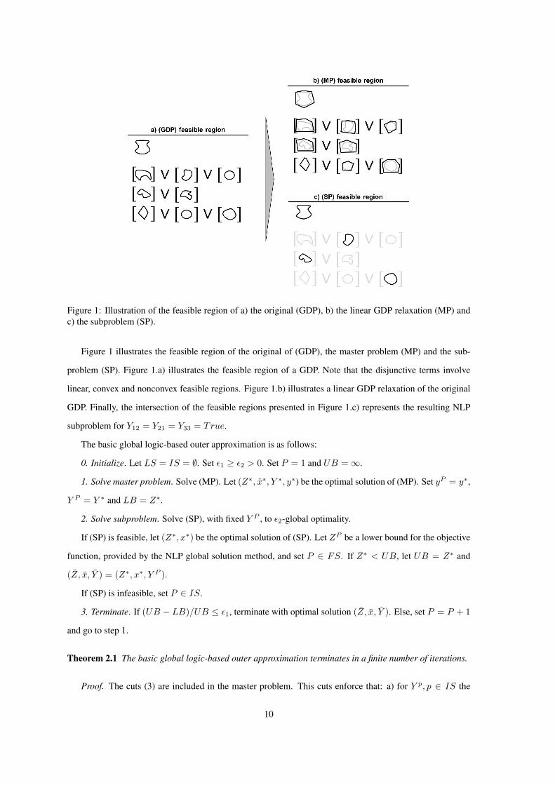
Figure 1: Illustration of the feasible region of a) the original (GDP), b) the linear GDP relaxation (MP) andc) the subproblem (SP).

Figure 1 illustrates the feasible region of the original of (GDP), the master problem (MP) and the sub-

problem (SP). Figure 1.a) illustrates the feasible region of a GDP. Note that the disjunctive terms involve

linear, convex and nonconvex feasible regions. Figure 1.b) illustrates a linear GDP relaxation of the original

GDP. Finally, the intersection of the feasible regions presented in Figure 1.c) represents the resulting NLP

subproblem for Y12 = Y21 = Y33 = True.

The basic global logic-based outer approximation is as follows:

0. Initialize. Let LS = IS = ∅. Set ε1 ≥ ε2 > 0. Set P = 1 and UB =∞.

1. Solve master problem. Solve (MP). Let (Z∗, x∗, Y ∗, y∗) be the optimal solution of (MP). Set yP = y∗,

Y P = Y ∗ and LB = Z∗.

2. Solve subproblem. Solve (SP), with fixed Y P , to ε2-global optimality.

If (SP) is feasible, let (Z∗, x∗) be the optimal solution of (SP). Let ZP be a lower bound for the objective

function, provided by the NLP global solution method, and set P ∈ FS. If Z∗ < UB, let UB = Z∗ and

(Z, x, Y ) = (Z∗, x∗, Y P ).

If (SP) is infeasible, set P ∈ IS.

3. Terminate. If (UB − LB)/UB ≤ ε1, terminate with optimal solution (Z, x, Y ). Else, set P = P + 1

and go to step 1.

Theorem 2.1 The basic global logic-based outer approximation terminates in a finite number of iterations.

Proof. The cuts (3) are included in the master problem. This cuts enforce that: a) for Y p, p ∈ IS the

10

master problem will be infeasible; b) for Y p, p ∈ FS the optimal solution of the master problem will beZ∗ ≥

Zp. This means that if all the Y p solutions that are feasible for (MP) are evaluated, then LB ≥ minp∈FS

Zp. (SP)

is solved to ε2-global optimality, so (UB − minp∈FS

Zp)/UB ≤ ε2. Since ε1 ≥ ε2, then (UB −LB)/UB ≤ ε1

.

3 Improved Global Logic-based Outer Approximation

The basic global logic-based outer approximation terminates in a finite number of iterations, but the conver-

gence can be slow. In this section we present two enhancements: one is to find feasible solutions faster, and

another one is to improve the lower bound provided by the master problem.

3.1 Two-phase Algorithm to improve Upper Bound

The basic global logic-based outer approximation requires the solution of the NLP subproblem to global

optimality. Therefore, it is possible that the algorithm takes a very long time even in the first iteration. In

order to evaluate many iterations, it is possible to modify the algorithm and consider a relatively short time

limit for the solution of the subproblem (τsub−limit). The step 2 of the algorithm can be modified as follows:

2. Solve subproblem. Solve (SP), with fixed Y P and time limit τsub−limit, using a global optimization

method.

If (SP) is proven infeasible, set P ∈ IS.

If at least one feasible solution for (SP) is found, let (Z∗, x∗) be the best feasible solution found for (MP).

Let ZP be a lower bound for the objective function, provided by the NLP global solution method, and set

P ∈ FS. If Z∗ < UB, let UB = Z∗ and (Z, x, Y ) = (Z∗, x∗, Y P ).

If no feasible solution is found, but (SP) is not proven infeasible, let ZP be a lower bound for the objective

function provided by the NLP global solution method. Set P ∈ FS.

This modification of the algorithm allows to evaluate several different alternatives in a short period of

time, assuming that the lower bound of the subproblems is still higher than the lower bound of the master

problem. The downside of this modified algorithm as that it does not necessarily terminate in a finite number

of iterations. In order to ensure that the algorithm terminates, the global logic-based outer approximation

can be divided into two phases. The first phase is the modified version with a time limit for solving the

subproblem. The second phase is the basic global logic-based outer approximation described in the previous

section.

Note that this enhancement is useful when the solution to global optimality of the subproblem is the

most time consuming step. It considers that the solution of the master problem (linear GDP) is “easy” in

11

comparison. Considering that the master problem can be solved as an MILP, and that MILP solvers have

become considerably efficient, this is usually true. Furthermore, in the synthesis of process networks the

nonlinear terms associated to the operation can be highly nonconvex. Therefore, solving an NLP with few

units can be difficult to be handled by NLP global solvers. On the other hand, a linear GDP with a few

hundred alternative units (e.g. a few hundred binary variables in the MILP reformulation) can typically be

easily handled by MILP solvers.

An additional enhancement to the two-phase algorithm is to diversify the search of feasible solutions

in the first phase. The reason for this is that the no-good-cuts (3) avoid the evaluation of the exact same

alternative, but the cuts have no effect if there is just one difference in an alternative (vs. the alternatives

previously evaluated). In order to search for more diverse solutions, the objective function in the first phase

can be modified as follows:

min Z −W∑

p=1,...,P−1

∑ypki=0

(yki) +∑ypki=1

(1− yki)

(4)

where W is a positive weighting parameter.

The modification of the objective function in (4) promotes the search for solutions that are “very different”

from previously evaluated alternatives. This penalty term is only included in the first phase. Note that the

algorithm has to be slightly modified in step 1 to ensure a valid lower bound, so the lower bound becomes

LB = Z∗ −W∑p=1,...,P

(∑ypki=0(y∗ki) +

∑ypki=1(1− y∗ki)

)instead of LB = Z∗.

3.2 Cutting Planes to improve Lower Bound

The no-good-cuts (3) ensure the termination of the algorithm in a finite number of iterations. However, these

cuts are useful only in avoiding the evaluation of previous solutions, and they normally do not have much

impact in improving the lower bound. For this reason, we propose a new method to derive valid cuts that help

to improve the lower bound.

The main objective of the proposed method is to derive linear inequalities that help to represent better

the individual feasible region of the selected disjunctive terms. In the synthesis of process networks these

linear inequalities will try to improve the linear representation of the nonconvex operating region of each

unit. These linear inequalities will be obtained through a separation problem, extending the approach of

Stubbs and Mehrotra[39] to nonconvex feasible regions. The cuts will be based on the strongest possible

convex envelope (i.e. the convex hull) of the complete feasible region of the disjunctive term.

For clarity purposes, we first present the case in which the cut by Stubbs and Mehrotra[39] can be directly

applied. Consider that, for a disjunctive term that was selected by the master problem (Y P ), a nonlinear

convex relaxation is available (rki(x) ≤ 0). Consider that this convex relaxation is stronger than the linear

12

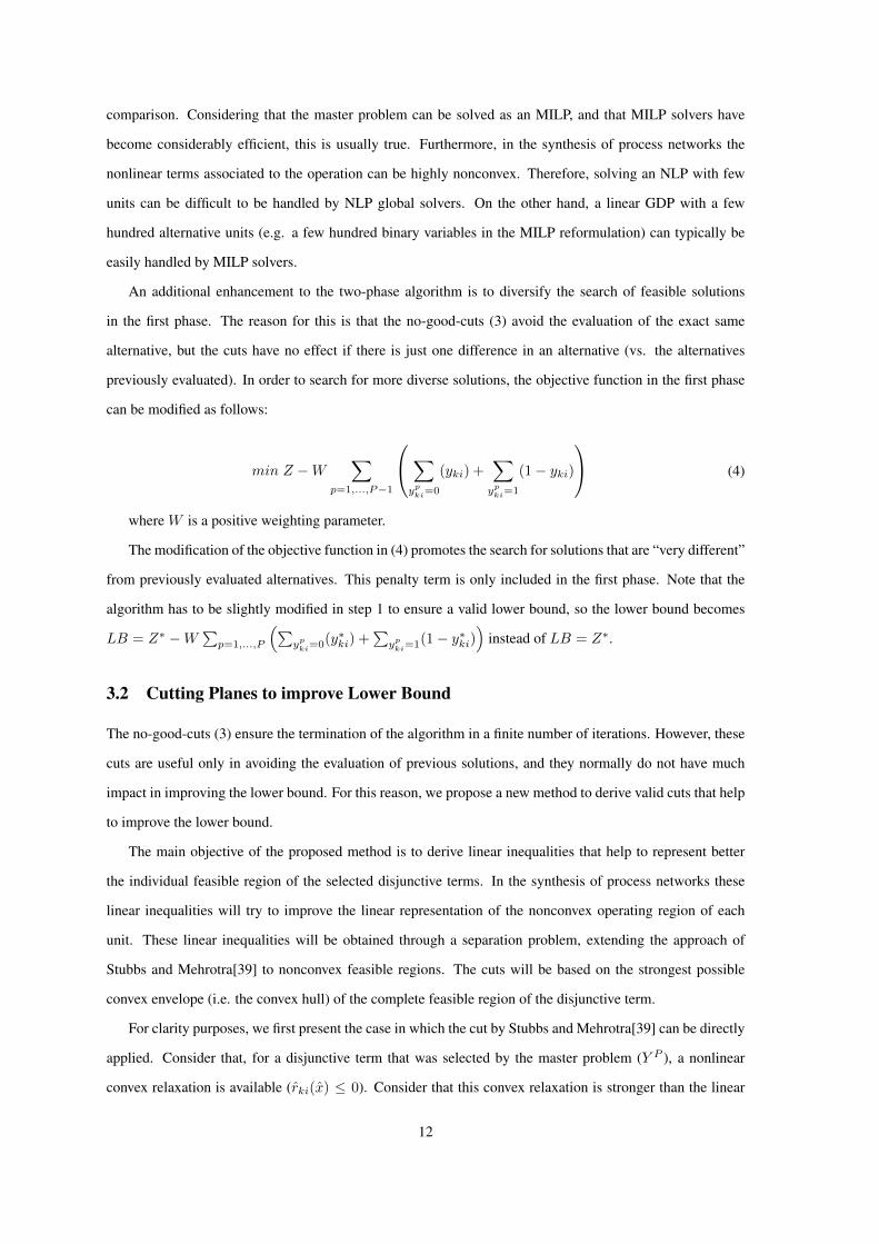
relaxation, so it is possible to establish the following relations on the feasible region of the selected term:

(rki(x) ≤ 0) ⊆ (rki(x) ≤ 0) ⊆ (Bkix ≤ bki), where xlo ≤ x ≤ xup, x = (x, xaux), xlo = (xlo, xloaux),

and xup = (xup, xupaux). Figure 2.a) illustrates these three feasible regions, projected into the original space

x.

Let x∗ be the solution of the master problem at iteration P . Let Y Pki = True be a selected disjunctive

term at iteration P , and assume that a nonlinear convex relaxation, that is stronger than the linear relaxation,

is available for that term (rki(x) ≤ 0). It is then possible to obtain cuts in the original space x, that separate

a point in x∗ from the feasible region rki(x) ≤ 0, using the following separation problem[39]:

min ||x− x∗||22

s.t. rki(x) ≤ 0

xlo ≤ x ≤ xup

x ∈ Rn+s

(5)

where x = (x, xaux).

Note that (5) is a convex NLP. Let xPki be the value of x at the optimal solution of (5). Then the following

inequality is a valid cut for rki(x) ≤ 0.

(ξPki)T

(x− xPki) ≥ 0 (6)

where ξPki = 2(xPki − x∗).

Inequality (6) lies in the original space of the variables x, and it is valid for any convex region rki(x) ≤ 0

[39]. Because (rki(x) ≤ 0) ⊆ (rki(x) ≤ 0), it is also valid for rki(x) ≤ 0. Note that the objective function in

(5) evaluates the distance using the square of the Euclidean norm, which provides a good cut and an analytical

expression for the subgradient ξPki. Any other norm also provides a valid cut, but the subgradient ξPki has to be

adjusted accordingly. The separation problem (5), and the cut generated from it (6) are illustrated in Figure

2.b) (projected into the original space x).

In order to obtain the cut, it is necessary to solve (5), which requires the knowledge of a convex relaxation

of the problem. However, we present an alternative separation problem that not only allows to obtain a cut

without rki(x) ≤ 0, but it also derives the cut using the strongest possible convex envelope of rki(x) ≤ 0

(i.e. its convex hull). The new separation problem is as follows:

13

Figure 2: Illustration of the feasible region and cuts generated for rki(x) ≤ 0, rki(x) ≤ 0, and Bkix ≤ bki;projected into the original space.

min ||x− x∗||22

s.t. x = λx1 + (1− λ)x2

rki(x1) ≤ 0

rki(x2) ≤ 0

xlo ≤ x1, x2 ≤ xup

0 ≤ λ ≤ 0.5

(7)

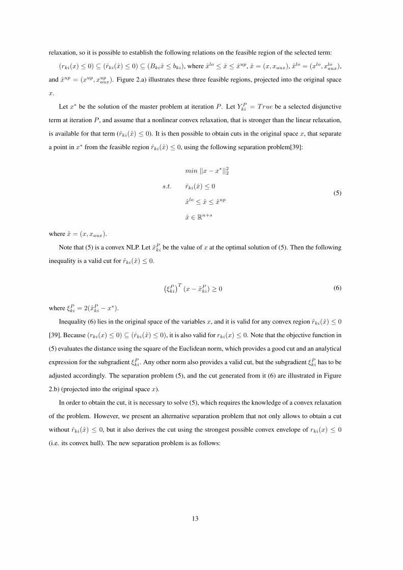
Theorem 3.1 The projection of the feasible region of (7) into the original space of x is the convex hull of the

feasible region described by rki(x) ≤ 0 and xlo ≤ x ≤ xup.

The proof of Theorem 3.1 is trivial. The feasible region of (7) describes x as a convex combination of

two points, both of which satisfy rki(x) ≤ 0 and xlo ≤ x ≤ xup (which is the description of the convex hull

itself). The feasible region of (7), projected into the original space, is illustrated in Figure 3.a).

Since the projection of the feasible region of (7) into the original space is convex, the inequality (6) is

also a valid cut if xPki is set as the value of x at the optimal solution of (7). The cut generated using separation

problem (7) is illustrated in Figure 3.b).

Separation problem (7) provides a tool for generating linear cuts that separate a point x∗ from the convex

hull of the feasible region of a selected disjunctive term (Yki = True). The main downside of (7) is that it is

nonconvex since it involves rki(x1), rki(x2) that can be noconvex, and the bilinear terms in x = λx1 + (1−

λ)x2. Furthermore, in order to obtain a valid cut it is necessary to solve (7) to global optimality. Even though

(7) can be difficult to solve, it is important to consider that: a) (7) is solved for an individual disjunctive term,

which normally involves a small fraction of the total number of constraints of the original problem; and b)

14

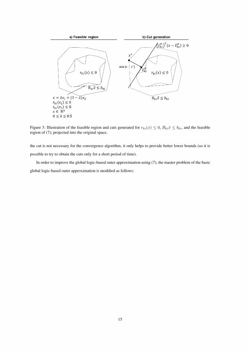
Figure 3: Illustration of the feasible region and cuts generated for rki(x) ≤ 0, Bkix ≤ bki, and the feasibleregion of (7); projected into the original space.

the cut is not necessary for the convergence algorithm, it only helps to provide better lower bounds (so it is

possible to try to obtain the cuts only for a short period of time).

In order to improve the global logic-based outer approximation using (7), the master problem of the basic

global logic-based outer approximation is modified as follows:

15

min Z

s.t. Z ≥ cTx

Ax ≤ a

∨i∈Dk

Yki

yki = 1

Bkix ≤ bki(ξPki)T

(x− xPki) ≥ 0 ∀p ∈ CCki

k ∈ K

Yi∈Dk

Yki k ∈ K

∑i∈Dk

yki = 1 k ∈ K

Ω(Y ) = True

Z ≥ (Zp − LB)

1−∑ypki=1

(yki)−∑ypki=0

(1− yki)

+ LB p ∈ FS

∑ypki=0

(yki) +∑ypki=1

(1− yki) ≥ 0 p ∈ IS

xlo ≤ x ≤ xup

x ∈ Rn+s

0 ≤ yki ≤ 1 k ∈ K, i ∈ Dk

Yki ∈ True, False k ∈ K, i ∈ Dk

(MP2)

where(ξPki)T

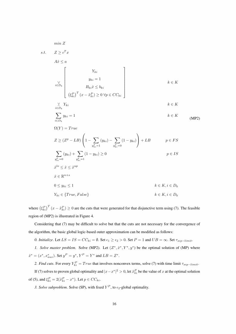
(x− xPki) ≥ 0 are the cuts that were generated for that disjunctive term using (7). The feasible

region of (MP2) is illustrated in Figure 4.

Considering that (7) may be difficult to solve but that the cuts are not necessary for the convergence of

the algorithm, the basic global logic-based outer approximation can be modified as follows:

0. Initialize. Let LS = IS = CCki = ∅. Set ε1 ≥ ε2 > 0. Set P = 1 and UB =∞. Set τsep−limit.

1. Solve master problem. Solve (MP2). Let (Z∗, x∗, Y ∗, y∗) be the optimal solution of (MP) where

x∗ = (x∗, x∗aux). Set yP = y∗, Y P = Y ∗ and LB = Z∗.

2. Find cuts. For every Y Pki = True that involves nonconvex terms, solve (7) with time limit τsep−limit.

If (7) solves to proven global optimality and |x−x∗|2 > 0, let xPki be the value of x at the optimal solution

of (5), and ξPki = 2(xPki − x∗). Let p ∈ CCki.

3. Solve subproblem. Solve (SP), with fixed Y P , to ε2-global optimality.

16

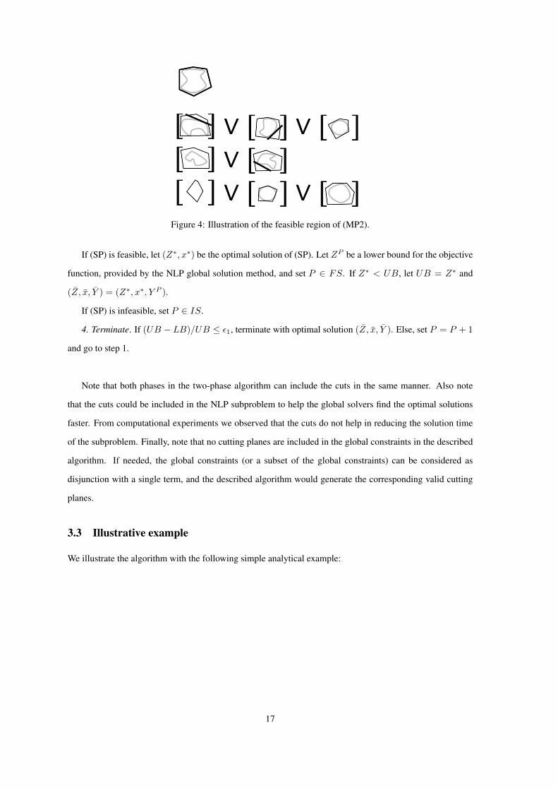
Figure 4: Illustration of the feasible region of (MP2).

If (SP) is feasible, let (Z∗, x∗) be the optimal solution of (SP). Let ZP be a lower bound for the objective

function, provided by the NLP global solution method, and set P ∈ FS. If Z∗ < UB, let UB = Z∗ and

(Z, x, Y ) = (Z∗, x∗, Y P ).

If (SP) is infeasible, set P ∈ IS.

4. Terminate. If (UB − LB)/UB ≤ ε1, terminate with optimal solution (Z, x, Y ). Else, set P = P + 1

and go to step 1.

Note that both phases in the two-phase algorithm can include the cuts in the same manner. Also note

that the cuts could be included in the NLP subproblem to help the global solvers find the optimal solutions

faster. From computational experiments we observed that the cuts do not help in reducing the solution time

of the subproblem. Finally, note that no cutting planes are included in the global constraints in the described

algorithm. If needed, the global constraints (or a subset of the global constraints) can be considered as

disjunction with a single term, and the described algorithm would generate the corresponding valid cutting

planes.

3.3 Illustrative example

We illustrate the algorithm with the following simple analytical example:

17

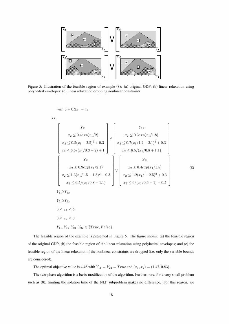
Figure 5: Illustration of the feasible region of example (8): (a) original GDP; (b) linear relaxation usingpolyhedral envelopes; (c) linear relaxation dropping nonlinear constraints.

min 5 + 0.2x1 − x2

s.t.

Y11

x2 ≤ 0.4exp(x1/2)

x2 ≤ 0.5(x1 − 2.5)2 + 0.3

x2 ≤ 6.5/(x1/0.3 + 2) + 1

∨

Y12

x2 ≤ 0.3exp(x1/1.8)

x2 ≤ 0.7(x1/1.2− 2.1)2 + 0.3

x2 ≤ 6.5/(x1/0.8 + 1.1)

Y21

x2 ≤ 0.9exp(x1/2.1)

x2 ≤ 1.3(x1/1.5− 1.8)2 + 0.3

x2 ≤ 6.5/(x1/0.8 + 1.1)

∨

Y22

x2 ≤ 0.4exp(x1/1.5)

x2 ≤ 1.2(x1/− 2.5)2 + 0.3

x2 ≤ 6/(x1/0.6 + 1) + 0.5

Y11YY12

Y21YY22

0 ≤ x1 ≤ 5

0 ≤ x2 ≤ 3

Y11, Y12, Y21, Y22 ∈ True, False

(8)

The feasible region of the example is presented in Figure 5. The figure shows: (a) the feasible region

of the original GDP; (b) the feasible region of the linear relaxation using polyhedral envelopes; and (c) the

feasible region of the linear relaxation if the nonlinear constraints are dropped (i.e. only the variable bounds

are considered).

The optimal objective value is 4.46 with Y11 = Y22 = True and (x1, x2) = (1.47, 0.83).

The two-phase algorithm is a basic modification of the algorithm. Furthermore, for a very small problem

such as (8), limiting the solution time of the NLP subproblem makes no difference. For this reason, we

18

illustrate the algorithm and derivation of cutting planes with a one-phase algorithm.

0. Initialize. Let LS = IS = CCki = ∅. ε1 = 0.1; ε2 = 0.005. Set P = 1 and UB =∞. Set τsep−limit.

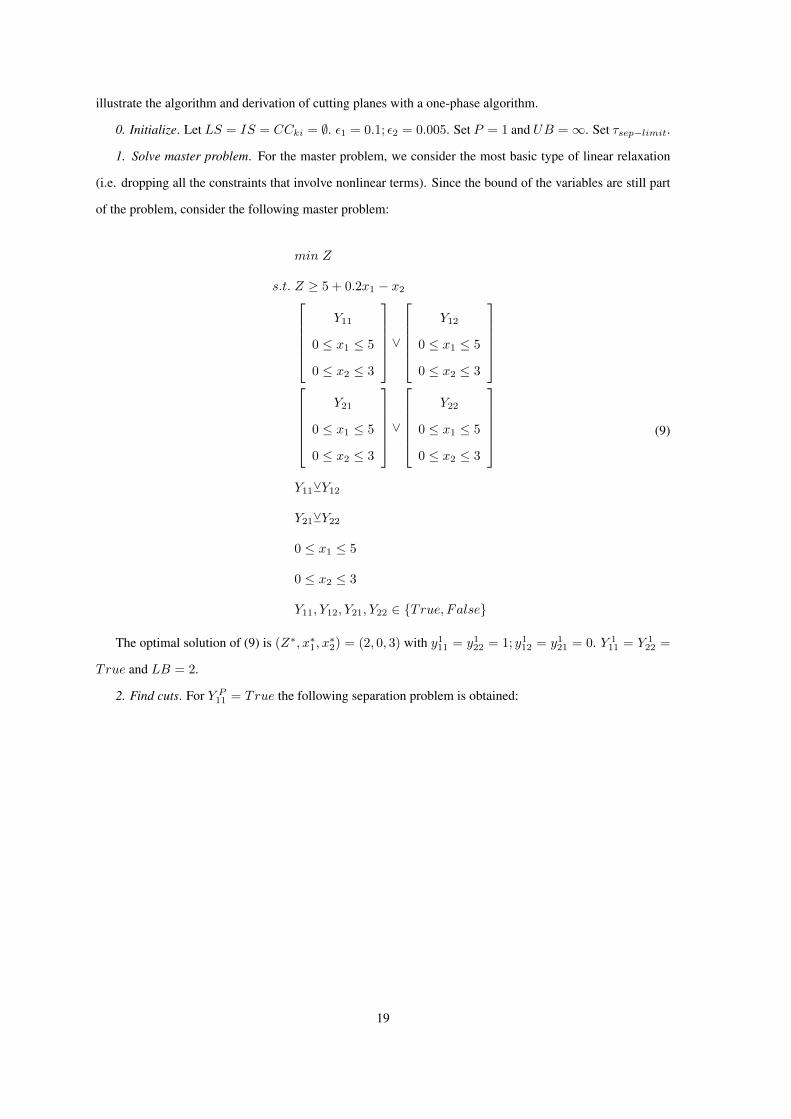
1. Solve master problem. For the master problem, we consider the most basic type of linear relaxation

(i.e. dropping all the constraints that involve nonlinear terms). Since the bound of the variables are still part

of the problem, consider the following master problem:

min Z

s.t. Z ≥ 5 + 0.2x1 − x2Y11

0 ≤ x1 ≤ 5

0 ≤ x2 ≤ 3

∨

Y12

0 ≤ x1 ≤ 5

0 ≤ x2 ≤ 3

Y21

0 ≤ x1 ≤ 5

0 ≤ x2 ≤ 3

∨

Y22

0 ≤ x1 ≤ 5

0 ≤ x2 ≤ 3

Y11YY12

Y21YY22

0 ≤ x1 ≤ 5

0 ≤ x2 ≤ 3

Y11, Y12, Y21, Y22 ∈ True, False

(9)

The optimal solution of (9) is (Z∗, x∗1, x∗2) = (2, 0, 3) with y111 = y122 = 1; y112 = y121 = 0. Y 1

11 = Y 122 =

True and LB = 2.

2. Find cuts. For Y P11 = True the following separation problem is obtained:

19

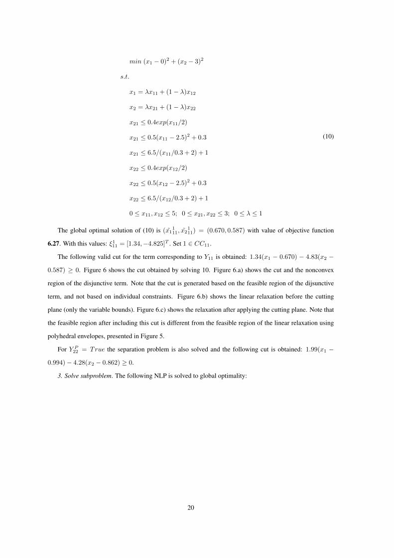
min (x1 − 0)2 + (x2 − 3)2

s.t.

x1 = λx11 + (1− λ)x12

x2 = λx21 + (1− λ)x22

x21 ≤ 0.4exp(x11/2)

x21 ≤ 0.5(x11 − 2.5)2 + 0.3

x21 ≤ 6.5/(x11/0.3 + 2) + 1

x22 ≤ 0.4exp(x12/2)

x22 ≤ 0.5(x12 − 2.5)2 + 0.3

x22 ≤ 6.5/(x12/0.3 + 2) + 1

0 ≤ x11, x12 ≤ 5; 0 ≤ x21, x22 ≤ 3; 0 ≤ λ ≤ 1

(10)

The global optimal solution of (10) is (x1111, x2

111) = (0.670, 0.587) with value of objective function

6.27. With this values: ξ111 = [1.34,−4.825]T . Set 1 ∈ CC11.

The following valid cut for the term corresponding to Y11 is obtained: 1.34(x1 − 0.670) − 4.83(x2 −

0.587) ≥ 0. Figure 6 shows the cut obtained by solving 10. Figure 6.a) shows the cut and the nonconvex

region of the disjunctive term. Note that the cut is generated based on the feasible region of the dijsunctive

term, and not based on individual constraints. Figure 6.b) shows the linear relaxation before the cutting

plane (only the variable bounds). Figure 6.c) shows the relaxation after applying the cutting plane. Note that

the feasible region after including this cut is different from the feasible region of the linear relaxation using

polyhedral envelopes, presented in Figure 5.

For Y P22 = True the separation problem is also solved and the following cut is obtained: 1.99(x1 −

0.994)− 4.28(x2 − 0.862) ≥ 0.

3. Solve subproblem. The following NLP is solved to global optimality:

20

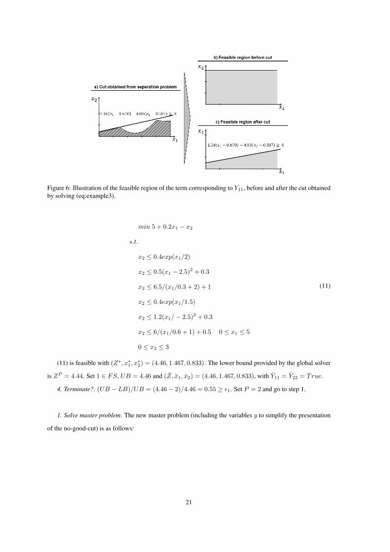
Figure 6: Illustration of the feasible region of the term corresponding to Y11, before and after the cut obtainedby solving (eq:example3).

min 5 + 0.2x1 − x2

s.t.

x2 ≤ 0.4exp(x1/2)

x2 ≤ 0.5(x1 − 2.5)2 + 0.3

x2 ≤ 6.5/(x1/0.3 + 2) + 1

x2 ≤ 0.4exp(x1/1.5)

x2 ≤ 1.2(x1/− 2.5)2 + 0.3

x2 ≤ 6/(x1/0.6 + 1) + 0.5 0 ≤ x1 ≤ 5

0 ≤ x2 ≤ 3

(11)

(11) is feasible with (Z∗, x∗1, x∗2) = (4.46, 1.467, 0.833). The lower bound provided by the global solver

is ZP = 4.44. Set 1 ∈ FS, UB = 4.46 and (Z, x1, x2) = (4.46, 1.467, 0.833), with Y11 = Y22 = True.

4. Terminate?. (UB − LB)/UB = (4.46− 2)/4.46 = 0.55 ≥ ε1. Set P = 2 and go to step 1.

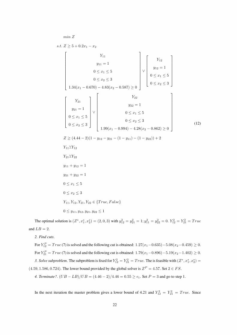
1. Solve master problem. The new master problem (including the variables y to simplify the presentation

of the no-good-cut) is as follows:

21

min Z

s.t. Z ≥ 5 + 0.2x1 − x2

Y11

y11 = 1

0 ≤ x1 ≤ 5

0 ≤ x2 ≤ 3

1.34(x1 − 0.670)− 4.83(x2 − 0.587) ≥ 0

∨

Y12

y12 = 1

0 ≤ x1 ≤ 5

0 ≤ x2 ≤ 3

Y21

y21 = 1

0 ≤ x1 ≤ 5

0 ≤ x2 ≤ 3

∨

Y22

y22 = 1

0 ≤ x1 ≤ 5

0 ≤ x2 ≤ 3

1.99(x1 − 0.994)− 4.28(x2 − 0.862) ≥ 0

Z ≥ (4.44− 2)(1− y12 − y21 − (1− y11)− (1− y22)) + 2

Y11YY12

Y21YY22

y11 + y12 = 1

y21 + y22 = 1

0 ≤ x1 ≤ 5

0 ≤ x2 ≤ 3

Y11, Y12, Y21, Y22 ∈ True, False

0 ≤ y11, y12, y21, y22 ≤ 1

(12)

The optimal solution is (Z∗, x∗1, x∗2) = (2, 0, 3) with y212 = y221 = 1; y211 = y222 = 0. Y 2

12 = Y 221 = True

and LB = 2.

2. Find cuts.

For Y P12 = True (7) is solved and the following cut is obtained: 1.27(x1−0.635)−5.08(x2−0.459) ≥ 0.

For Y P21 = True (7) is solved and the following cut is obtained: 1.79(x1−0.896)−5.19(x2−1.402) ≥ 0.

3. Solve subproblem. The subproblem is fixed for Y 212 = Y 2

21 = True. The is feasible with (Z∗, x∗1, x∗2) =

(4.59, 1.586, 0.724). The lower bound provided by the global solver is ZP = 4.57. Set 2 ∈ FS.

4. Terminate?. (UB − LB)/UB = (4.46− 2)/4.46 = 0.55 ≥ ε1. Set P = 3 and go to step 1.

In the next iteration the master problem gives a lower bound of 4.21 and Y 212 = Y 2

21 = True. Since

22

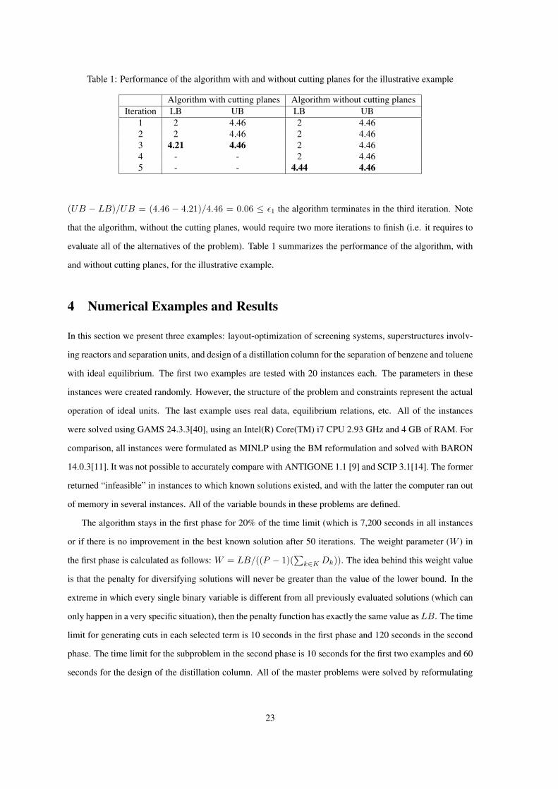
Table 1: Performance of the algorithm with and without cutting planes for the illustrative example

Algorithm with cutting planes Algorithm without cutting planesIteration LB UB LB UB

1 2 4.46 2 4.462 2 4.46 2 4.463 4.21 4.46 2 4.464 - - 2 4.465 - - 4.44 4.46

(UB − LB)/UB = (4.46 − 4.21)/4.46 = 0.06 ≤ ε1 the algorithm terminates in the third iteration. Note

that the algorithm, without the cutting planes, would require two more iterations to finish (i.e. it requires to

evaluate all of the alternatives of the problem). Table 1 summarizes the performance of the algorithm, with

and without cutting planes, for the illustrative example.

4 Numerical Examples and Results

In this section we present three examples: layout-optimization of screening systems, superstructures involv-

ing reactors and separation units, and design of a distillation column for the separation of benzene and toluene

with ideal equilibrium. The first two examples are tested with 20 instances each. The parameters in these

instances were created randomly. However, the structure of the problem and constraints represent the actual

operation of ideal units. The last example uses real data, equilibrium relations, etc. All of the instances

were solved using GAMS 24.3.3[40], using an Intel(R) Core(TM) i7 CPU 2.93 GHz and 4 GB of RAM. For

comparison, all instances were formulated as MINLP using the BM reformulation and solved with BARON

14.0.3[11]. It was not possible to accurately compare with ANTIGONE 1.1 [9] and SCIP 3.1[14]. The former

returned “infeasible” in instances to which known solutions existed, and with the latter the computer ran out

of memory in several instances. All of the variable bounds in these problems are defined.

The algorithm stays in the first phase for 20% of the time limit (which is 7,200 seconds in all instances

or if there is no improvement in the best known solution after 50 iterations. The weight parameter (W ) in

the first phase is calculated as follows: W = LB/((P − 1)(∑k∈K Dk)). The idea behind this weight value

is that the penalty for diversifying solutions will never be greater than the value of the lower bound. In the

extreme in which every single binary variable is different from all previously evaluated solutions (which can

only happen in a very specific situation), then the penalty function has exactly the same value asLB. The time

limit for generating cuts in each selected term is 10 seconds in the first phase and 120 seconds in the second

phase. The time limit for the subproblem in the second phase is 10 seconds for the first two examples and 60

seconds for the design of the distillation column. All of the master problems were solved by reformulating

23

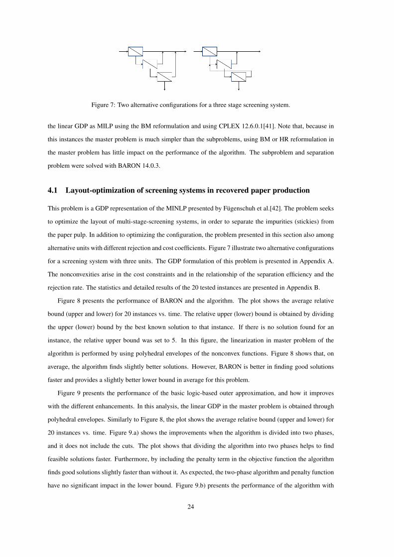
Figure 7: Two alternative configurations for a three stage screening system.

the linear GDP as MILP using the BM reformulation and using CPLEX 12.6.0.1[41]. Note that, because in

this instances the master problem is much simpler than the subproblems, using BM or HR reformulation in

the master problem has little impact on the performance of the algorithm. The subproblem and separation

problem were solved with BARON 14.0.3.

4.1 Layout-optimization of screening systems in recovered paper production

This problem is a GDP representation of the MINLP presented by Fugenschuh et al.[42]. The problem seeks

to optimize the layout of multi-stage-screening systems, in order to separate the impurities (stickies) from

the paper pulp. In addition to optimizing the configuration, the problem presented in this section also among

alternative units with different rejection and cost coefficients. Figure 7 illustrate two alternative configurations

for a screening system with three units. The GDP formulation of this problem is presented in Appendix A.

The nonconvexities arise in the cost constraints and in the relationship of the separation efficiency and the

rejection rate. The statistics and detailed results of the 20 tested instances are presented in Appendix B.

Figure 8 presents the performance of BARON and the algorithm. The plot shows the average relative

bound (upper and lower) for 20 instances vs. time. The relative upper (lower) bound is obtained by dividing

the upper (lower) bound by the best known solution to that instance. If there is no solution found for an

instance, the relative upper bound was set to 5. In this figure, the linearization in master problem of the

algorithm is performed by using polyhedral envelopes of the nonconvex functions. Figure 8 shows that, on

average, the algorithm finds slightly better solutions. However, BARON is better in finding good solutions

faster and provides a slightly better lower bound in average for this problem.

Figure 9 presents the performance of the basic logic-based outer approximation, and how it improves

with the different enhancements. In this analysis, the linear GDP in the master problem is obtained through

polyhedral envelopes. Similarly to Figure 8, the plot shows the average relative bound (upper and lower) for

20 instances vs. time. Figure 9.a) shows the improvements when the algorithm is divided into two phases,

and it does not include the cuts. The plot shows that dividing the algorithm into two phases helps to find

feasible solutions faster. Furthermore, by including the penalty term in the objective function the algorithm

finds good solutions slightly faster than without it. As expected, the two-phase algorithm and penalty function

have no significant impact in the lower bound. Figure 9.b) presents the performance of the algorithm with

24

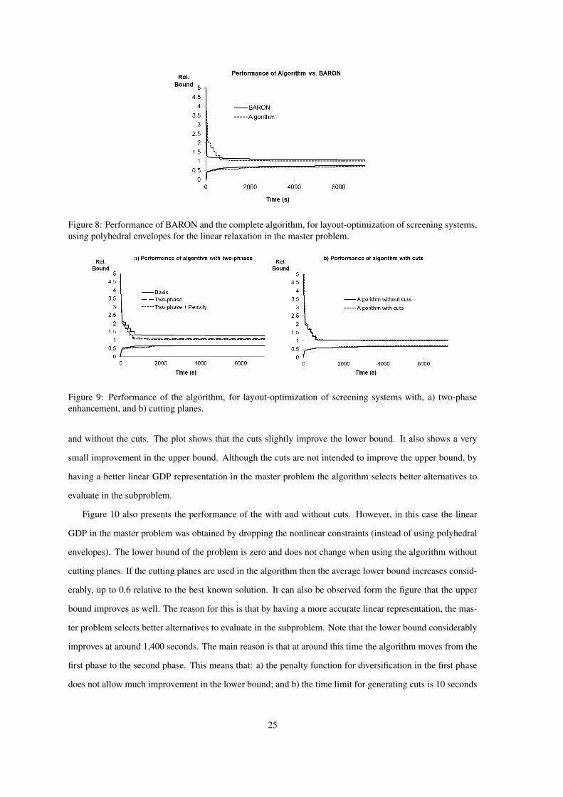
Figure 8: Performance of BARON and the complete algorithm, for layout-optimization of screening systems,using polyhedral envelopes for the linear relaxation in the master problem.

Figure 9: Performance of the algorithm, for layout-optimization of screening systems with, a) two-phaseenhancement, and b) cutting planes.

and without the cuts. The plot shows that the cuts slightly improve the lower bound. It also shows a very

small improvement in the upper bound. Although the cuts are not intended to improve the upper bound, by

having a better linear GDP representation in the master problem the algorithm selects better alternatives to

evaluate in the subproblem.

Figure 10 also presents the performance of the with and without cuts. However, in this case the linear

GDP in the master problem was obtained by dropping the nonlinear constraints (instead of using polyhedral

envelopes). The lower bound of the problem is zero and does not change when using the algorithm without

cutting planes. If the cutting planes are used in the algorithm then the average lower bound increases consid-

erably, up to 0.6 relative to the best known solution. It can also be observed form the figure that the upper

bound improves as well. The reason for this is that by having a more accurate linear representation, the mas-

ter problem selects better alternatives to evaluate in the subproblem. Note that the lower bound considerably

improves at around 1,400 seconds. The main reason is that at around this time the algorithm moves from the

first phase to the second phase. This means that: a) the penalty function for diversification in the first phase

does not allow much improvement in the lower bound; and b) the time limit for generating cuts is 10 seconds

25

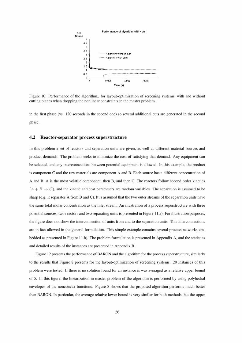
Figure 10: Performance of the algorithm,, for layout-optimization of screening systems, with and withoutcutting planes when dropping the nonlinear constraints in the master problem.

in the first phase (vs. 120 seconds in the second one) so several additional cuts are generated in the second

phase.

4.2 Reactor-separator process superstructure

In this problem a set of reactors and separation units are given, as well as different material sources and

product demands. The problem seeks to minimize the cost of satisfying that demand. Any equipment can

be selected, and any interconnections between potential equipment is allowed. In this example, the product

is component C and the raw materials are component A and B. Each source has a different concentration of

A and B. A is the most volatile component, then B, and then C. The reactors follow second order kinetics

(A + B → C), and the kinetic and cost parameters are random variables. The separation is assumed to be

sharp (e.g. it separates A from B and C). It is assumed that the two outer streams of the separation units have

the same total molar concentration as the inlet stream. An illustration of a process superstructure with three

potential sources, two reactors and two separating units is presented in Figure 11.a). For illustration purposes,

the figure does not show the interconnection of units from and to the separation units. This interconnections

are in fact allowed in the general formulation. This simple example contains several process networks em-

bedded as presented in Figure 11.b). The problem formulation is presented in Appendix A, and the statistics

and detailed results of the instances are presented in Appendix B.

Figure 12 presents the performance of BARON and the algorithm for the process superstructure, similarly

to the results that Figure 8 presents for the layout-optimization of screening systems. 20 instances of this

problem were tested. If there is no solution found for an instance is was averaged as a relative upper bound

of 5. In this figure, the linearization in master problem of the algorithm is performed by using polyhedral

envelopes of the nonconvex functions. Figure 8 shows that the proposed algorithm performs much better

than BARON. In particular, the average relative lower bound is very similar for both methods, but the upper

26

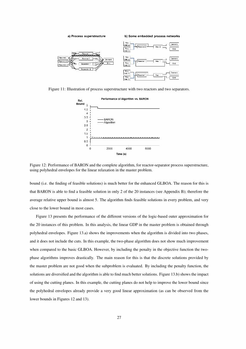
Figure 11: Illustration of process superstructure with two reactors and two separators.

Figure 12: Performance of BARON and the complete algorithm, for reactor-separator process superstructure,using polyhedral envelopes for the linear relaxation in the master problem.

bound (i.e. the finding of feasible solutions) is much better for the enhanced GLBOA. The reason for this is

that BARON is able to find a feasible solution in only 2 of the 20 instances (see Appendix B); therefore the

average relative upper bound is almost 5. The algorithm finds feasible solutions in every problem, and very

close to the lower bound in most cases.

Figure 13 presents the performance of the different versions of the logic-based outer approximation for

the 20 instances of this problem. In this analysis, the linear GDP in the master problem is obtained through

polyhedral envelopes. Figure 13.a) shows the improvements when the algorithm is divided into two phases,

and it does not include the cuts. In this example, the two-phase algorithm does not show much improvement

when compared to the basic GLBOA. However, by including the penalty in the objective function the two-

phase algorithms improves drastically. The main reason for this is that the discrete solutions provided by

the master problem are not good when the subproblem is evaluated. By including the penalty function, the

solutions are diversified and the algorithm is able to find much better solutions. Figure 13.b) shows the impact

of using the cutting planes. In this example, the cutting planes do not help to improve the lower bound since

the polyhedral envelopes already provide a very good linear approximation (as can be observed from the

lower bounds in Figures 12 and 13).

27

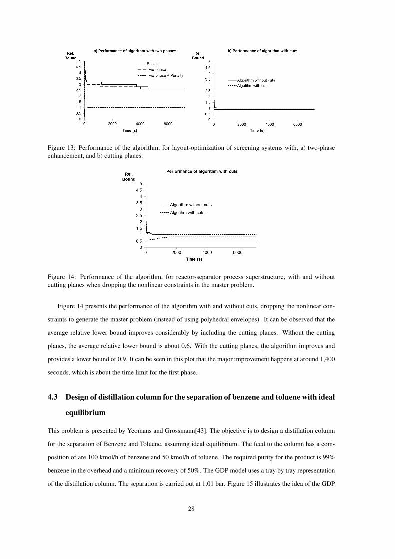
Figure 13: Performance of the algorithm, for layout-optimization of screening systems with, a) two-phaseenhancement, and b) cutting planes.

Figure 14: Performance of the algorithm, for reactor-separator process superstructure, with and withoutcutting planes when dropping the nonlinear constraints in the master problem.

Figure 14 presents the performance of the algorithm with and without cuts, dropping the nonlinear con-

straints to generate the master problem (instead of using polyhedral envelopes). It can be observed that the

average relative lower bound improves considerably by including the cutting planes. Without the cutting

planes, the average relative lower bound is about 0.6. With the cutting planes, the algorithm improves and

provides a lower bound of 0.9. It can be seen in this plot that the major improvement happens at around 1,400

seconds, which is about the time limit for the first phase.

4.3 Design of distillation column for the separation of benzene and toluene with ideal

equilibrium

This problem is presented by Yeomans and Grossmann[43]. The objective is to design a distillation column

for the separation of Benzene and Toluene, assuming ideal equilibrium. The feed to the column has a com-

position of are 100 kmol/h of benzene and 50 kmol/h of toluene. The required purity for the product is 99%

benzene in the overhead and a minimum recovery of 50%. The GDP model uses a tray by tray representation

of the distillation column. The separation is carried out at 1.01 bar. Figure 15 illustrates the idea of the GDP

28

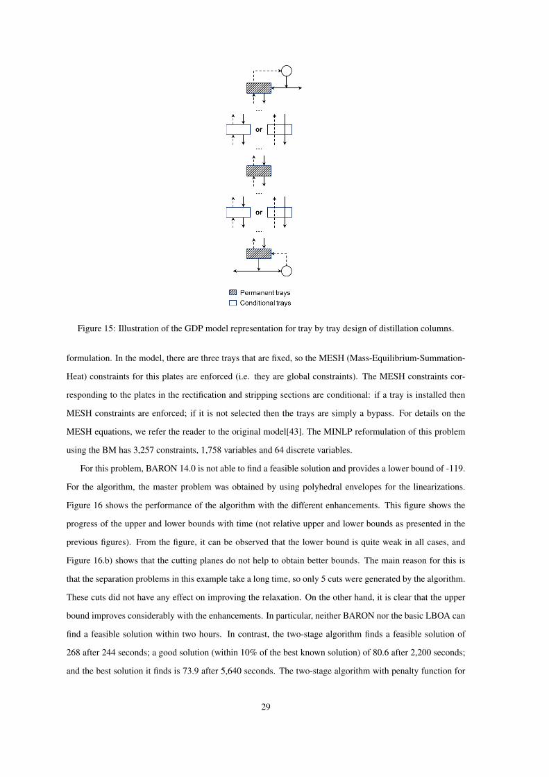
Figure 15: Illustration of the GDP model representation for tray by tray design of distillation columns.

formulation. In the model, there are three trays that are fixed, so the MESH (Mass-Equilibrium-Summation-

Heat) constraints for this plates are enforced (i.e. they are global constraints). The MESH constraints cor-

responding to the plates in the rectification and stripping sections are conditional: if a tray is installed then

MESH constraints are enforced; if it is not selected then the trays are simply a bypass. For details on the

MESH equations, we refer the reader to the original model[43]. The MINLP reformulation of this problem

using the BM has 3,257 constraints, 1,758 variables and 64 discrete variables.

For this problem, BARON 14.0 is not able to find a feasible solution and provides a lower bound of -119.

For the algorithm, the master problem was obtained by using polyhedral envelopes for the linearizations.

Figure 16 shows the performance of the algorithm with the different enhancements. This figure shows the

progress of the upper and lower bounds with time (not relative upper and lower bounds as presented in the

previous figures). From the figure, it can be observed that the lower bound is quite weak in all cases, and

Figure 16.b) shows that the cutting planes do not help to obtain better bounds. The main reason for this is

that the separation problems in this example take a long time, so only 5 cuts were generated by the algorithm.

These cuts did not have any effect on improving the relaxation. On the other hand, it is clear that the upper

bound improves considerably with the enhancements. In particular, neither BARON nor the basic LBOA can

find a feasible solution within two hours. In contrast, the two-stage algorithm finds a feasible solution of

268 after 244 seconds; a good solution (within 10% of the best known solution) of 80.6 after 2,200 seconds;

and the best solution it finds is 73.9 after 5,640 seconds. The two-stage algorithm with penalty function for

29

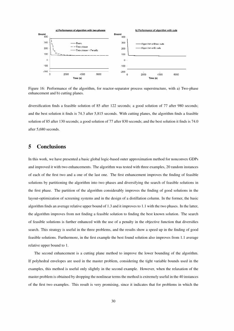
Figure 16: Performance of the algorithm, for reactor-separator process superstructure, with a) Two-phaseenhancement and b) cutting planes.

diversification finds a feasible solution of 85 after 122 seconds; a good solution of 77 after 980 seconds;

and the best solution it finds is 74.3 after 5,815 seconds. With cutting planes, the algorithm finds a feasible

solution of 85 after 130 seconds; a good solution of 77 after 830 seconds; and the best solution it finds is 74.0

after 5,680 seconds.

5 Conclusions

In this work, we have presented a basic global logic-based outer approximation method for nonconvex GDPs

and improved it with two enhancements. The algorithm was tested with three examples, 20 random instances

of each of the first two and a one of the last one. The first enhancement improves the finding of feasible

solutions by partitioning the algorithm into two phases and diversifying the search of feasible solutions in

the first phase. The partition of the algorithm considerably improves the finding of good solutions in the

layout-optimization of screening systems and in the design of a distillation column. In the former, the basic

algorithm finds an average relative upper bound of 1.3 and it improves to 1.1 with the two phases. In the latter,

the algorithm improves from not finding a feasible solution to finding the best known solution. The search

of feasible solutions is further enhanced with the use of a penalty in the objective function that diversifies

search. This strategy is useful in the three problems, and the results show a speed up in the finding of good

feasible solutions. Furthermore, in the first example the best found solution also improves from 1.1 average

relative upper bound to 1.

The second enhancement is a cutting plane method to improve the lower bounding of the algorithm.

If polyhedral envelopes are used in the master problem, considering the tight variable bounds used in the

examples, this method is useful only slightly in the second example. However, when the relaxation of the

master problem is obtained by dropping the nonlinear terms the method is extremely useful in the 40 instances

of the first two examples. This result is very promising, since it indicates that for problems in which the

30

linear relaxation is poor the method can derive strong cutting planes that will considerably improve the linear

approximation. Note that if the bounds of the variables are poor the polyhedral envelopes will tend to be poor

as well. However, the cutting planes obtained through the method presented in this work depend only on the

feasible region of the disjunctive term (e.g. processing units). This means that as long as the feasible region

is the same, the cutting planes obtained through the method are the same regardless of the variable bounds.

Acknowledgments

The authors would like to acknowledge financial support from the Center for Advanced Process Decision-

making (CAPD).

References

[1] Grossmann, I. E. Mixed-integer programming approach for the synthesis of integrated process flow-

sheets. Computers & chemical engineering 1985, 9, 463–482.

[2] Grossmann, I. E. Mixed-integer nonlinear programming techniques for the synthesis of engineering

systems. Research in Engineering Design 1990, 1, 205–228.

[3] Friedler, F; Tarjan, K; Huang, Y.; Fan, L. Graph-theoretic approach to process synthesis: axioms and

theorems. Chemical Engineering Science 1992, 47, 1973–1988.

[4] Smith, E.; Pantelides, C. Design of reaction/separation networks using detailed models. Computers &

chemical engineering 1995, 19, 83–88.

[5] Papalexandri, K. P.; Pistikopoulos, E. N. Generalized modular representation framework for process

synthesis. AIChE Journal 1996, 42, 1010–1032.

[6] Yeomans, H.; Grossmann, I. E. A systematic modeling framework of superstructure optimization in

process synthesis. Computers & Chemical Engineering 1999, 23, 709–731.

[7] Horst, R.; Tuy, H. Global optimization: Deterministic approaches; Springer Science & Business Me-

dia, 1996.

[8] Adjiman, C. S.; Androulakis, I. P.; Floudas, C. A. A global optimization method, αBB, for gen-

eral twice-differentiable constrained NLPsII. Implementation and computational results. Computers

& Chemical Engineering 1998, 22, 1159–1179.

[9] Misener, R.; Floudas, C. A. ANTIGONE: algorithms for continuous/integer global optimization of

nonlinear equations. Journal of Global Optimization 2014, 59, 503–526.

31

[10] Sahinidis, N. V. BARON: A general purpose global optimization software package. Journal of global

optimization 1996, 8, 201–205.

[11] Tawarmalani, M.; Sahinidis, N. V. A polyhedral branch-and-cut approach to global optimization. Math-

ematical Programming 2005, 103, 225–249.

[12] Belotti, P.; Lee, J.; Liberti, L.; Margot, F.; Wachter, A. Branching and bounds tighteningtechniques for

non-convex MINLP. Optimization Methods & Software 2009, 24, 597–634.

[13] Lin, Y.; Schrage, L. The global solver in the LINDO API. Optimization Methods & Software 2009, 24,

657–668.

[14] Achterberg, T. SCIP: solving constraint integer programs. Mathematical Programming Computation

2009, 1, 1–41.

[15] Bussieck, M. R.; Vigerske, S. MINLP solver software. Wiley Encyclopedia of Operations Research

and Management Science 2010.

[16] Kesavan, P.; Allgor, R. J.; Gatzke, E. P.; Barton, P. I. Outer approximation algorithms for separable

nonconvex mixed-integer nonlinear programs. Mathematical Programming 2004, 100, 517–535.

[17] Duran, M. A.; Grossmann, I. E. An outer-approximation algorithm for a class of mixed-integer non-

linear programs. Mathematical programming 1986, 36, 307–339.

[18] Fletcher, R.; Leyffer, S. Solving mixed integer nonlinear programs by outer approximation. Mathemat-

ical programming 1994, 66, 327–349.

[19] Hooker, J. N.; Ottosson, G. Logic-based Benders decomposition. Mathematical Programming 2003,

96, 33–60.

[20] Benders, J. F. Partitioning procedures for solving mixed-variables programming problems. Numerische

mathematik 1962, 4, 238–252.

[21] Geoffrion, A. M. Generalized benders decomposition. Journal of optimization theory and applications

1972, 10, 237–260.

[22] Li, X.; Tomasgard, A.; Barton, P. I. Nonconvex generalized Benders decomposition for stochastic

separable mixed-integer nonlinear programs. Journal of optimization theory and applications 2011,

151, 425–454.

[23] Raman, R.; Grossmann, I. E. Modelling and computational techniques for logic based integer pro-

gramming. Computers & Chemical Engineering 1994, 18, 563–578.

[24] Grossmann, I. E.; Trespalacios, F. Systematic modeling of discrete-continuous optimization models

through generalized disjunctive programming. AIChE Journal 2013, 59, 3276–3295.

32

[25] Raman, R.; Grossmann, I. E. Symbolic integration of logic in mixed-integer linear programming tech-

niques for process synthesis. Computers & Chemical Engineering 1993, 17, 909–927.

[26] Wolsey, L. A.; Nemhauser, G. L. Integer and combinatorial optimization; John Wiley & Sons, 2014.

[27] Lee, S.; Grossmann, I. E. New algorithms for nonlinear generalized disjunctive programming. Com-

puters & Chemical Engineering 2000, 24, 2125–2141.

[28] Lee, S.; Grossmann, I. E. Logic-based modeling and solution of nonlinear discrete/continuous opti-

mization problems. Annals of Operations Research 2005, 139, 267–288.

[29] Turkay, M.; Grossmann, I. E. Logic-based MINLP algorithms for the optimal synthesis of process

networks. Computers & Chemical Engineering 1996, 20, 959–978.

[30] Bergamini, M. L.; Aguirre, P.; Grossmann, I. Logic-based outer approximation for globally optimal

synthesis of process networks. Computers & chemical engineering 2005, 29, 1914–1933.

[31] Smith, E. M.; Pantelides, C. C. A symbolic reformulation/spatial branch-and-bound algorithm for the

global optimisation of nonconvex MINLPs. Computers & Chemical Engineering 1999, 23, 457–478.

[32] McCormick, G. P. Computability of global solutions to factorable nonconvex programs: Part IConvex

underestimating problems. Mathematical programming 1976, 10, 147–175.

[33] Tawarmalani, M.; Sahinidis, N. V. Convexification and global optimization in continuous and mixed-

integer nonlinear programming: theory, algorithms, software, and applications; Springer Science &

Business Media, 2002; Vol. 65.

[34] Adjiman, C. S.; Dallwig, S.; Floudas, C. A.; Neumaier, A. A global optimization method, αBB, for

general twice-differentiable constrained NLPsI. Theoretical advances. Computers & Chemical Engi-

neering 1998, 22, 1137–1158.

[35] Grossmann, I. E.; Lee, S. Generalized convex disjunctive programming: Nonlinear convex hull relax-

ation. Computational Optimization and Applications 2003, 26, 83–100.

[36] Williams, H. P. Model building in mathematical programming; John Wiley & Sons, 2013.

[37] Sawaya, N. Reformulations, relaxations and cutting planes for generalized disjunctive programming,

2006; Vol. 67.

[38] Trespalacios, F.; Grossmann, I. E. Review of Mixed-Integer Nonlinear and Generalized Disjunctive

Programming Methods. Chemie Ingenieur Technik 2014, 86, 991–1012.

[39] Stubbs, R. A.; Mehrotra, S. A branch-and-cut method for 0-1 mixed convex programming. Mathemat-

ical Programming 1999, 86, 515–532.

[40] Brooke, A.; Kendrick, D.; Meeraus, A.; Raman GAMS, a Users Guide. The Scientific Press 1998.

33

[41] CPLEX, I. I. V12. 1: Users Manual for CPLEX. International Business Machines Corporation 2009,

46, 157.

[42] Fugenschuh, A.; Hayn, C.; Michaels, D. Mixed-integer linear methods for layout-optimization of

screening systems in recovered paper production. Optimization and Engineering 2014, 15, 533–573.

[43] Yeomans, H.; Grossmann, I. E. Disjunctive programming models for the optimal design of distillation

columns and separation sequences. Industrial & Engineering Chemistry Research 2000, 39, 1637–

1648.

A Appendix A: GDP formulations of numerical examples

A.1 GDP formulation for layout-optimization of screening systems in recovered pa-

per production.

Nomenclature:

SETS:

J = fib, st Components (fibre is the “good component” and stickies is the “bad component”).

N = S ∪ ta, tr: Total nodes in the system (possible screens, total accept, and total reject).

S: Possible screens.

PARAMETERS (all parameters are greek letters or capital letters):

αs: Exponent coefficient for cost in screen s

βs,j : Acceptance factor beta for screen s and component j.

C1s : Cost coefficient 1 for screen s.

C2s : Cost coefficient 2 for screen s.

Cupst : Maximum percentage of inlet stickies accepted in the total accepted flow.

F 0j : Source flow of component j.

[F in,los , F in,ups ]: Lower and upper bound of flow into screen s.

W 1,W 2,W 3: Weighting factors in objective function for lost fire, accepted stickies, and capital cost

respectively.

CONTINUOUS (POSITIVE) VARIABLES:

cs: Cost of screen s.

fs: Total inlet flow into screen s.

f In,j : Inlet flow of component j into node n.

fAs,j : Accepted flow of component j from screen s.

fRs,j : Rejected flow of component j form screen s.

34

mAs,n,j : Accepted flow of component j from screen s to node n.

mRs,n,j : Rejected flow of component j from screen s to node n.

m0n,j : Flow of component j from source to node n.

rs: Reject rate of screen s.

BOOLEAN VARIABLES:

Ys: Selection of screen s.

Y As,n: Existence of accepted flow from screen s to node n.

Y Rs,n: Existence of rejected flow from screen s to node n.

Y 0n: Existence of flow from source to node n.

GDP model:

35

min W 1f Itr,fib +W 2f Ita,st +W 3∑s∈S

cs

s.t. f Ita,st ≤ Cupst F

0st

f Is,j = fAs,j + fRs,j s ∈ S, j ∈ J

fs =∑j∈J

f Is,j s ∈ S

f In,j = m0n,j +

∑s∈Ss 6=n

(mAs,n,j +mR

s,n,j

)n ∈ N, j ∈ J

F 0j =

∑n∈N

m0n,j j ∈ J

Ys

F in,los ≤ f Is ≤ F in,ups

fRs,j = f Is,j(rs)βs,j j ∈ J

cs = C1s (f Is )αs + C2

s (1− rs)

∨

¬Ys

f Is = 0

cs = 0

s ∈ S

Y As,n

mAs,n,j = fAs,j j ∈ J

∨ ¬Y As,n

mAs,n,j = 0 j ∈ J

s ∈ S, n ∈ N,n 6= s

Y Rs,n

mRs,n,j = fRs,j j ∈ J

∨ ¬Y Rs,n

mRs,n,j = 0 j ∈ J

s ∈ S, n ∈ N,n 6= s

∨n∈N

Y 0n

m0n,j = F 0

j j ∈ J

m0n′,j = 0 n′ 6= n, j ∈ J

Y

n∈NY 0n

Y As,n ∨ Y Rs,n ⇒ Ys s ∈ S, n ∈ N,n 6= s

Y As′,s ∨ Y Rs′,s ⇒ Ys (s, s′) ∈ S, s′ 6= s

Y As′,s Y Y As,s′ (s, s′) ∈ S, s′ 6= s

Y Rs′,s Y Y Rs,s′ (s, s′) ∈ S, s′ 6= s

Y As,n Y Y Rs,n s ∈ S, n ∈ N,n 6= s

Y As,n Y Y Rs,n s ∈ S, n ∈ N,n 6= s

(13)

A.2 GDP formulation for reactor-separator process superstructure.

Nomenclature:

SETS:

36

I: Components (a, b, c).

K = R ∪ S: Total processing units.

R: Reactors.

S: Separation units.

P : Sources of raw materials.

PARAMETERS:

Raw materials.

C0p,i: Molar concentration of component i in raw material p.

PR0p: Cost of raw material p.

F 0,upp : Maximum availability of raw material p.

Demand.

MDc : Minimum mol fraction of component c in demand stream.

FD: Minimum demand (total flow).

Separation:

ξs,i ∈ 0, 1: ξs,i = 1 of component i exits outlet stream out1 in separation process s. ξs,i = 0 of

component i exits outlet stream out2.

Reactors:

γr: Minimum concentration ratio between component a and b.

kr: Reaction rate constant for reactor r.

rr: Design residence time for reactor r.

All units:

αk: Cost coefficient for unit k.

βk: Cost exponent for unit k.

PP 0k,k′ : Cost of installing a pipeline between unit k and unit k′.

Variable bounds:

[F lok , Fupk ]: Lower and upper bound of total flow into unit k.

[Clok,i, Cupk,i]: Lower and upper bound of molar concentration of i into unit k.

[µlok,k′ , µupk,k′ ]: Lower and upper bound of total flow from unit k into unit k′.

[νlok,k′,i, νupk,k′,i]: Lower and upper bound of molar concentration of component i in stream from unit k into

unit k′.

CONTINUOUS (POSITIVE) VARIABLES:

F ink : Inlet stream for unit k.

F outr : Outlet stream of reactor r.

F out1s , F out2s : Outlet streams 1 and 2 of separation unit s.

37

Cink,i: Molar concentration of i in the inlet stream for unit k.

Coutr,i : Molar concentration of i in the outlet stream of reactor r.

Cout1s,i , Cout2s,i : Molar concentration of i in the outlet streams (out1, out2) of unit s.

µr,k: Total flow from reactor r to unit k.

νr,k,i: Molar concentration of component i in stream from reactor r into unit k.

µout1s,k , µout2s,k : Total flow from outlet streams (out1, out2) of unit s to unit k.

νout1s,k,i , νout2s,k,i : Molar concentration of component i in stream from outlet streams (out1, out2) of unit s to

unit k.

µrawp,k : Flow of raw material from source p ro unit k.

µDr : Flow of outlet stream from reactor r to demand.

µout1,Ds , µout2,Ds : Flow of outlet streams (out1, out2) from separation unit s to demand.

νDr,i: Molar concentration of component i in flow of outlet stream from reactor r to demand.

νout1,Ds,i , µout2,Ds,i : Molar concentration of component i in flow of outlet streams (out1, out2) from sepa-

ration unit s to demand.

PUk: Cost of unit k.

PPk,k′ : Cost of pipeline from unit k to unit k′.

PUT , PPT , PRT : Total cost of units, pipelines and raw materials.

BOOLEAN VARIABLES:

Yk: selection of unit k.

Y Fr,k: Existence of flow between reactor r and unit k.

Y F out1s,k , Y F out2s,k : Existence of flow between outlet streams from separation unit s and unit k.

38

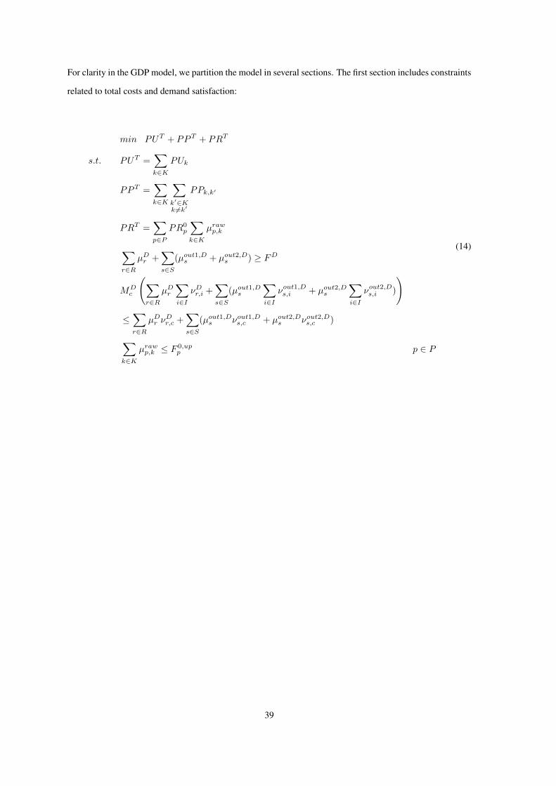
For clarity in the GDP model, we partition the model in several sections. The first section includes constraints

related to total costs and demand satisfaction:

min PUT + PPT + PRT

s.t. PUT =∑k∈K

PUk

PPT =∑k∈K

∑k′∈Kk 6=k′

PPk,k′

PRT =∑p∈P

PR0p

∑k∈K

µrawp,k

∑r∈R

µDr +∑s∈S

(µout1,Ds + µout2,Ds ) ≥ FD

MDc

(∑r∈R

µDr∑i∈I

νDr,i +∑s∈S

(µout1,Ds

∑i∈I

νout1,Ds,i + µout2,Ds

∑i∈I

νout2,Ds,i )

)

≤∑r∈R

µDr νDr,c +

∑s∈S

(µout1,Ds νout1,Ds,c + µout2,Ds νout2,Ds,c )

∑k∈K

µrawp,k ≤ F 0,upp p ∈ P

(14)

39

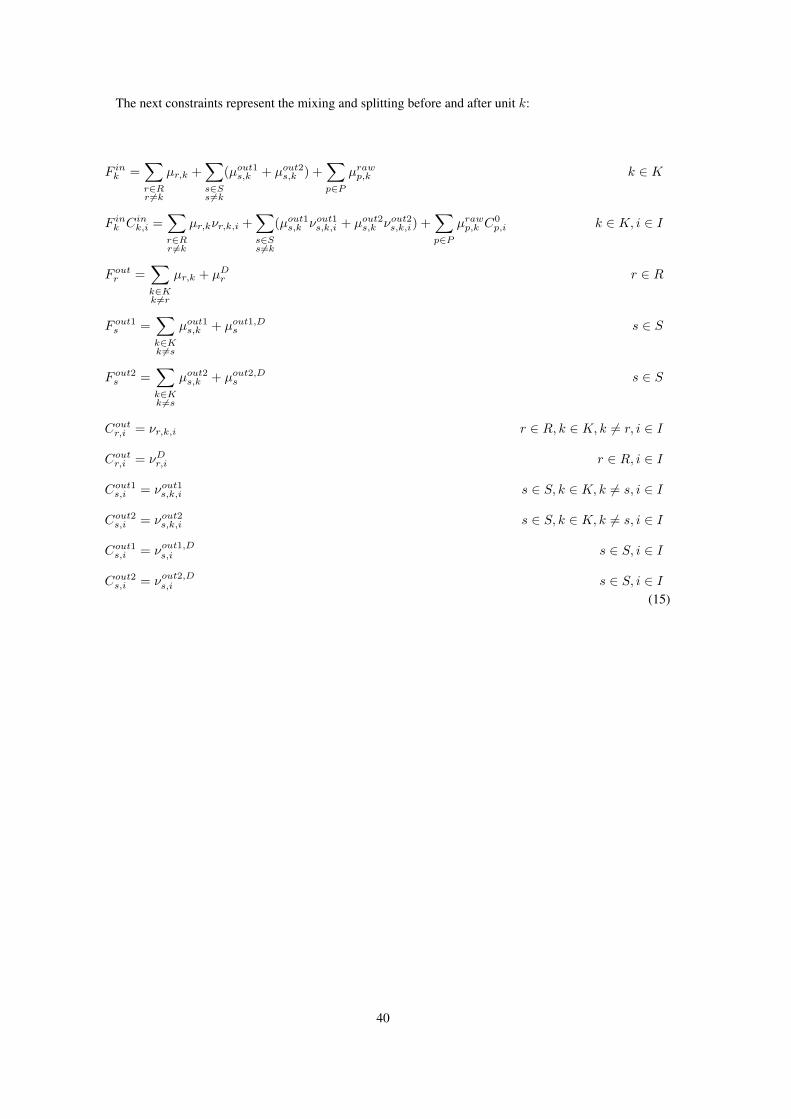
The next constraints represent the mixing and splitting before and after unit k:

F ink =∑r∈Rr 6=k

µr,k +∑s∈Ss6=k

(µout1s,k + µout2s,k ) +∑p∈P

µrawp,k k ∈ K

F ink Cink,i =∑r∈Rr 6=k

µr,kνr,k,i +∑s∈Ss6=k

(µout1s,k νout1s,k,i + µout2s,k νout2s,k,i) +∑p∈P

µrawp,k C0p,i k ∈ K, i ∈ I

F outr =∑k∈Kk 6=r

µr,k + µDr r ∈ R

F out1s =∑k∈Kk 6=s

µout1s,k + µout1,Ds s ∈ S

F out2s =∑k∈Kk 6=s

µout2s,k + µout2,Ds s ∈ S

Coutr,i = νr,k,i r ∈ R, k ∈ K, k 6= r, i ∈ I

Coutr,i = νDr,i r ∈ R, i ∈ I

Cout1s,i = νout1s,k,i s ∈ S, k ∈ K, k 6= s, i ∈ I

Cout2s,i = νout2s,k,i s ∈ S, k ∈ K, k 6= s, i ∈ I

Cout1s,i = νout1,Ds,i s ∈ S, i ∈ I

Cout2s,i = νout2,Ds,i s ∈ S, i ∈ I(15)

40

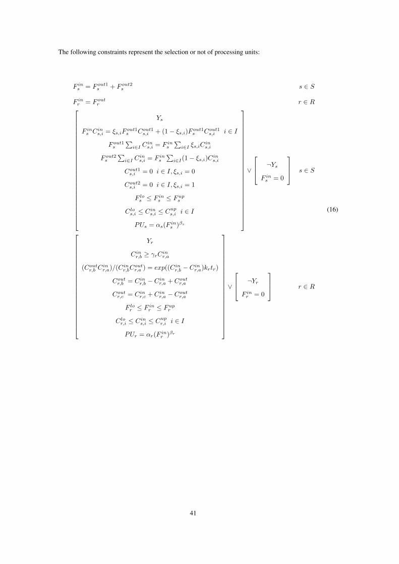
The following constraints represent the selection or not of processing units:

F ins = F out1s + F out2s s ∈ S

F inr = F outr r ∈ R

Ys

F ins Cins,i = ξs,iFout1s Cout1s,i + (1− ξs,i)F out1s Cout1s,i i ∈ I

F out1s

∑i∈I C

ins,i = F ins

∑i∈I ξs,iC

ins,i

F out2s

∑i∈I C

ins,i = F ins

∑i∈I(1− ξs,i)Cins,i

Cout1s,i = 0 i ∈ I, ξs,i = 0

Cout2s,i = 0 i ∈ I, ξs,i = 1

F los ≤ F ins ≤ Fups

Clos,i ≤ Cins,i ≤ Cups,i i ∈ I

PUs = αs(Fins )βs

∨

¬Ys

F ins = 0

s ∈ S

Yr

Cinr,b ≥ γrCinr,a

(Coutr,b Cinr,a)/(Cinr,bC

outr,a ) = exp((Cinr,b − Cinr,a)krtr)

Coutr,b = Cinr,b − Cinr,a + Coutr,a

Coutr,c = Cinr,c + Cinr,a − Coutr,a

F lor ≤ F inr ≤ Fupr

Clor,i ≤ Cins,i ≤ Cupr,i i ∈ I

PUr = αr(Finr )βr

∨

¬Yr

F inr = 0

r ∈ R

(16)

41

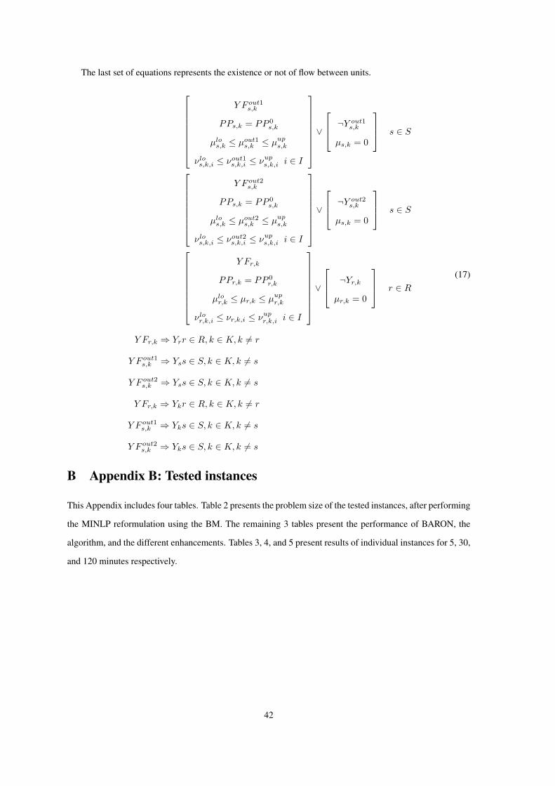
The last set of equations represents the existence or not of flow between units.

Y F out1s,k

PPs,k = PP 0s,k

µlos,k ≤ µout1s,k ≤ µups,k

νlos,k,i ≤ νout1s,k,i ≤ νups,k,i i ∈ I

∨

¬Y out1s,k

µs,k = 0

s ∈ S

Y F out2s,k

PPs,k = PP 0s,k

µlos,k ≤ µout2s,k ≤ µups,k

νlos,k,i ≤ νout2s,k,i ≤ νups,k,i i ∈ I

∨

¬Y out2s,k

µs,k = 0

s ∈ S

Y Fr,k

PPr,k = PP 0r,k

µlor,k ≤ µr,k ≤ µupr,k

νlor,k,i ≤ νr,k,i ≤ νupr,k,i i ∈ I

∨

¬Yr,k

µr,k = 0

r ∈ R

Y Fr,k ⇒ Yrr ∈ R, k ∈ K, k 6= r

Y F out1s,k ⇒ Yss ∈ S, k ∈ K, k 6= s

Y F out2s,k ⇒ Yss ∈ S, k ∈ K, k 6= s

Y Fr,k ⇒ Ykr ∈ R, k ∈ K, k 6= r

Y F out1s,k ⇒ Yks ∈ S, k ∈ K, k 6= s

Y F out2s,k ⇒ Yks ∈ S, k ∈ K, k 6= s

(17)

B Appendix B: Tested instances

This Appendix includes four tables. Table 2 presents the problem size of the tested instances, after performing

the MINLP reformulation using the BM. The remaining 3 tables present the performance of BARON, the

algorithm, and the different enhancements. Tables 3, 4, and 5 present results of individual instances for 5, 30,

and 120 minutes respectively.

42

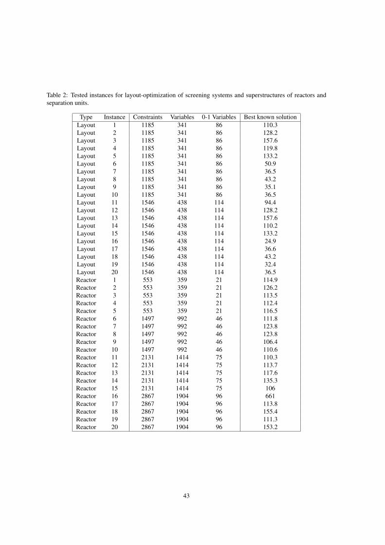
Table 2: Tested instances for layout-optimization of screening systems and superstructures of reactors andseparation units.

Type Instance Constraints Variables 0-1 Variables Best known solutionLayout 1 1185 341 86 110.3Layout 2 1185 341 86 128.2Layout 3 1185 341 86 157.6Layout 4 1185 341 86 119.8Layout 5 1185 341 86 133.2Layout 6 1185 341 86 50.9Layout 7 1185 341 86 36.5Layout 8 1185 341 86 43.2Layout 9 1185 341 86 35.1Layout 10 1185 341 86 36.5Layout 11 1546 438 114 94.4Layout 12 1546 438 114 128.2Layout 13 1546 438 114 157.6Layout 14 1546 438 114 110.2Layout 15 1546 438 114 133.2Layout 16 1546 438 114 24.9Layout 17 1546 438 114 36.6Layout 18 1546 438 114 43.2Layout 19 1546 438 114 32.4Layout 20 1546 438 114 36.5Reactor 1 553 359 21 114.9Reactor 2 553 359 21 126.2Reactor 3 553 359 21 113.5Reactor 4 553 359 21 112.4Reactor 5 553 359 21 116.5Reactor 6 1497 992 46 111.8Reactor 7 1497 992 46 123.8Reactor 8 1497 992 46 123.8Reactor 9 1497 992 46 106.4Reactor 10 1497 992 46 110.6Reactor 11 2131 1414 75 110.3Reactor 12 2131 1414 75 113.7Reactor 13 2131 1414 75 117.6Reactor 14 2131 1414 75 135.3Reactor 15 2131 1414 75 106Reactor 16 2867 1904 96 661Reactor 17 2867 1904 96 113.8Reactor 18 2867 1904 96 155.4Reactor 19 2867 1904 96 111.3Reactor 20 2867 1904 96 153.2

43

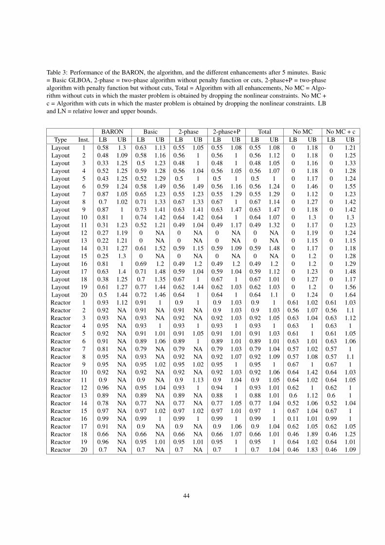
Table 3: Performance of the BARON, the algorithm, and the different enhancements after 5 minutes. Basic= Basic GLBOA, 2-phase = two-phase algorithm without penalty function or cuts, 2-phase+P = two-phasealgorithm with penalty function but without cuts, Total = Algorithm with all enhancements, No MC = Algo-rithm without cuts in which the master problem is obtained by dropping the nonlinear constraints. No MC +c = Algorithm with cuts in which the master problem is obtained by dropping the nonlinear constraints. LBand LN = relative lower and upper bounds.

BARON Basic 2-phase 2-phase+P Total No MC No MC + cType Inst. LB UB LB UB LB UB LB UB LB UB LB UB LB UB

Layout 1 0.58 1.3 0.63 1.13 0.55 1.05 0.55 1.08 0.55 1.08 0 1.18 0 1.21Layout 2 0.48 1.09 0.58 1.16 0.56 1 0.56 1 0.56 1.12 0 1.18 0 1.25Layout 3 0.33 1.25 0.5 1.23 0.48 1 0.48 1 0.48 1.05 0 1.16 0 1.33Layout 4 0.52 1.25 0.59 1.28 0.56 1.04 0.56 1.05 0.56 1.07 0 1.18 0 1.28Layout 5 0.43 1.25 0.52 1.29 0.5 1 0.5 1 0.5 1 0 1.17 0 1.24Layout 6 0.59 1.24 0.58 1.49 0.56 1.49 0.56 1.16 0.56 1.24 0 1.46 0 1.55Layout 7 0.87 1.05 0.65 1.23 0.55 1.23 0.55 1.29 0.55 1.29 0 1.12 0 1.23Layout 8 0.7 1.02 0.71 1.33 0.67 1.33 0.67 1 0.67 1.14 0 1.27 0 1.42Layout 9 0.87 1 0.73 1.41 0.63 1.41 0.63 1.47 0.63 1.47 0 1.18 0 1.42Layout 10 0.81 1 0.74 1.42 0.64 1.42 0.64 1 0.64 1.07 0 1.3 0 1.3Layout 11 0.31 1.23 0.52 1.21 0.49 1.04 0.49 1.17 0.49 1.32 0 1.17 0 1.23Layout 12 0.27 1.19 0 NA 0 NA 0 NA 0 NA 0 1.19 0 1.24Layout 13 0.22 1.21 0 NA 0 NA 0 NA 0 NA 0 1.15 0 1.15Layout 14 0.31 1.27 0.61 1.52 0.59 1.15 0.59 1.09 0.59 1.48 0 1.17 0 1.18Layout 15 0.25 1.3 0 NA 0 NA 0 NA 0 NA 0 1.2 0 1.28Layout 16 0.81 1 0.69 1.2 0.49 1.2 0.49 1.2 0.49 1.2 0 1.2 0 1.29Layout 17 0.63 1.4 0.71 1.48 0.59 1.04 0.59 1.04 0.59 1.12 0 1.23 0 1.48Layout 18 0.38 1.25 0.7 1.35 0.67 1 0.67 1 0.67 1.01 0 1.27 0 1.17Layout 19 0.61 1.27 0.77 1.44 0.62 1.44 0.62 1.03 0.62 1.03 0 1.2 0 1.56Layout 20 0.5 1.44 0.72 1.46 0.64 1 0.64 1 0.64 1.1 0 1.24 0 1.64Reactor 1 0.93 1.12 0.91 1 0.9 1 0.9 1.03 0.9 1 0.61 1.02 0.61 1.03Reactor 2 0.92 NA 0.91 NA 0.91 NA 0.9 1.03 0.9 1.03 0.56 1.07 0.56 1.1Reactor 3 0.93 NA 0.93 NA 0.92 NA 0.92 1.03 0.92 1.05 0.63 1.04 0.63 1.12Reactor 4 0.95 NA 0.93 1 0.93 1 0.93 1 0.93 1 0.63 1 0.63 1Reactor 5 0.92 NA 0.91 1.01 0.91 1.05 0.91 1.01 0.91 1.03 0.61 1 0.61 1.05Reactor 6 0.91 NA 0.89 1.06 0.89 1 0.89 1.01 0.89 1.01 0.63 1.01 0.63 1.06Reactor 7 0.81 NA 0.79 NA 0.79 NA 0.79 1.03 0.79 1.04 0.57 1.02 0.57 1Reactor 8 0.95 NA 0.93 NA 0.92 NA 0.92 1.07 0.92 1.09 0.57 1.08 0.57 1.1Reactor 9 0.95 NA 0.95 1.02 0.95 1.02 0.95 1 0.95 1 0.67 1 0.67 1Reactor 10 0.92 NA 0.92 NA 0.92 NA 0.92 1.03 0.92 1.06 0.64 1.42 0.64 1.03Reactor 11 0.9 NA 0.9 NA 0.9 1.13 0.9 1.04 0.9 1.05 0.64 1.02 0.64 1.05Reactor 12 0.96 NA 0.95 1.04 0.93 1 0.94 1 0.93 1.01 0.62 1 0.62 1Reactor 13 0.89 NA 0.89 NA 0.89 NA 0.88 1 0.88 1.01 0.6 1.12 0.6 1Reactor 14 0.78 NA 0.77 NA 0.77 NA 0.77 1.05 0.77 1.04 0.52 1.06 0.52 1.04Reactor 15 0.97 NA 0.97 1.02 0.97 1.02 0.97 1.01 0.97 1 0.67 1.04 0.67 1Reactor 16 0.99 NA 0.99 1 0.99 1 0.99 1 0.99 1 0.11 1.01 0.99 1Reactor 17 0.91 NA 0.9 NA 0.9 NA 0.9 1.06 0.9 1.04 0.62 1.05 0.62 1.05Reactor 18 0.66 NA 0.66 NA 0.66 NA 0.66 1.07 0.66 1.01 0.46 1.89 0.46 1.25Reactor 19 0.96 NA 0.95 1.01 0.95 1.01 0.95 1 0.95 1 0.64 1.02 0.64 1.01Reactor 20 0.7 NA 0.7 NA 0.7 NA 0.7 1 0.7 1.04 0.46 1.83 0.46 1.09

44

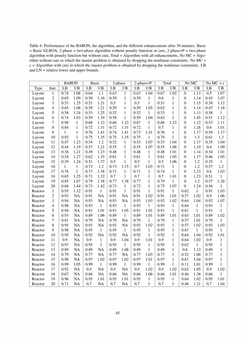
Table 4: Performance of the BARON, the algorithm, and the different enhancements after 30 minutes. Basic= Basic GLBOA, 2-phase = two-phase algorithm without penalty function or cuts, 2-phase+P = two-phasealgorithm with penalty function but without cuts, Total = Algorithm with all enhancements, No MC = Algo-rithm without cuts in which the master problem is obtained by dropping the nonlinear constraints. No MC +c = Algorithm with cuts in which the master problem is obtained by dropping the nonlinear constraints. LBand LN = relative lower and upper bounds.

BARON Basic 2-phase 2-phase+P Total No MC No MC + cType Inst. LB UB LB UB LB UB LB UB LB UB LB UB LB UB

Layout 1 0.74 1.08 0.64 1.1 0.63 1 0.63 1.04 0.67 1.02 0 1.13 0.5 1.07Layout 2 0.65 1.09 0.59 1.16 0.59 1 0.59 1 0.6 1 0 1.14 0.45 1.07Layout 3 0.53 1.25 0.51 1.21 0.5 1 0.5 1 0.51 1 0 1.15 0.38 1.12Layout 4 0.65 1.08 0.59 1.21 0.59 1 0.59 1.05 0.62 1 0 1.14 0.47 1.18Layout 5 0.58 1.24 0.53 1.25 0.52 1 0.52 1 0.53 1 0 1.13 0.38 1Layout 6 0.74 1.03 0.59 1.39 0.58 1 0.59 1.04 0.62 1 0 1.45 0.51 1.12Layout 7 0.98 1 0.68 1.23 0.66 1.23 0.67 1 0.66 1.23 0 1.12 0.53 1.11Layout 8 0.84 1 0.72 1.31 0.72 1.31 0.72 1 0.7 1 0 1.26 0.6 1.01Layout 9 1 1 0.76 1.41 0.74 1.41 0.73 1.41 0.76 1 0 1.17 0.58 1.17Layout 10 0.92 1 0.75 1.35 0.75 1.35 0.75 1 0.79 1 0 1.3 0.61 1.3Layout 11 0.47 1.23 0.54 1.2 0.52 1 0.53 1.07 0.53 1.04 0 1.17 0.35 1.04Layout 12 0.44 1.19 0.57 1.21 0.55 1 0.55 1.07 0.55 1.08 0 1.19 0.4 1.09Layout 13 0.36 1.21 0.49 1.23 0.48 1 0.48 1 0.48 1.01 0 1.14 0.34 1.01Layout 14 0.54 1.27 0.62 1.35 0.61 1 0.61 1 0.61 1.05 0 1.17 0.46 1.05Layout 15 0.39 1.24 0.51 1.37 0.5 1 0.5 1 0.5 1.06 0 1.2 0.35 1Layout 16 1 1 0.73 1.2 0.73 1.15 0.7 1.03 0.71 1 0 1.2 0.57 1.2Layout 17 0.78 1 0.73 1.38 0.71 1 0.71 1 0.74 1 0 1.23 0.6 1.03Layout 18 0.65 1.25 0.71 1.32 0.7 1 0.7 1 0.7 1.01 0 1.23 0.51 1Layout 19 0.85 1.07 0.79 1.38 0.77 1.38 0.77 1 0.79 1 0 1.2 0.57 1.26Layout 20 0.68 1.44 0.73 1.42 0.73 1 0.72 1 0.75 1.07 0 1.24 0.56 1Reactor 1 0.93 1.12 0.91 1 0.91 1 0.91 1 0.91 1 0.62 1 0.91 1.03Reactor 2 0.93 NA 0.91 NA 0.91 NA 0.91 1.02 0.91 1.01 0.57 1.02 0.9 1.06Reactor 3 0.94 NA 0.93 NA 0.93 NA 0.93 1.03 0.92 1.02 0.64 1.04 0.92 1.07Reactor 4 0.98 NA 0.93 1 0.93 1 0.93 1 0.93 1 0.64 1 0.93 1Reactor 5 0.94 NA 0.91 1.01 0.91 1.05 0.91 1.01 0.91 1 0.61 1 0.91 1Reactor 6 0.93 NA 0.89 1.06 0.89 1 0.89 1.01 0.89 1.01 0.63 1.01 0.89 1.02Reactor 7 0.81 NA 0.79 NA 0.79 NA 0.79 1 0.79 1 0.57 1.01 0.79 1Reactor 8 0.95 NA 0.93 NA 0.93 NA 0.93 1.02 0.93 1 0.57 1.02 0.93 1.03Reactor 9 0.98 NA 0.95 1 0.95 1 0.95 1 0.95 1 0.67 1 0.95 1Reactor 10 0.95 NA 0.92 NA 0.92 NA 0.92 1 0.92 1 0.64 1.04 0.92 1.01Reactor 11 0.9 NA 0.9 1 0.9 1.04 0.9 1.01 0.9 1 0.64 1.02 0.9 1Reactor 12 0.97 NA 0.95 1 0.95 1 0.95 1 0.95 1 0.62 1 0.95 1Reactor 13 0.89 NA 0.89 NA 0.89 1.08 0.89 1 0.89 1 0.6 1.12 0.89 1Reactor 14 0.79 NA 0.77 NA 0.77 NA 0.77 1.03 0.77 1 0.52 1.06 0.77 1Reactor 15 0.98 NA 0.97 1.02 0.97 1.02 0.97 1.01 0.97 1 0.67 1.04 0.97 1Reactor 16 0.99 1.05 0.99 1 0.99 1 0.99 1 0.99 1 0.11 1.01 0.99 1Reactor 17 0.92 NA 0.9 NA 0.9 NA 0.9 1.02 0.9 1.02 0.62 1.05 0.9 1.02Reactor 18 0.67 NA 0.66 NA 0.66 NA 0.66 1.06 0.66 1.01 0.46 1.36 0.66 1Reactor 19 0.96 NA 0.95 1.01 0.95 1.01 0.95 1 0.95 1 0.64 1.02 0.95 1.01Reactor 20 0.71 NA 0.7 NA 0.7 NA 0.7 1 0.7 1 0.46 1.21 0.7 1.04

45

Table 5: Performance of the BARON, the algorithm, and the different enhancements after 120 minutes.Basic = Basic GLBOA, 2-phase = two-phase algorithm without penalty function or cuts, 2-phase+P = two-phase algorithm with penalty function but without cuts, Total = Algorithm with all enhancements, No MC =Algorithm without cuts in which the master problem is obtained by dropping the nonlinear constraints. NoMC + c = Algorithm with cuts in which the master problem is obtained by dropping the nonlinear constraints.LB and LN = relative lower and upper bounds.

BARON Basic 2-phase 2-phase+P Total No MC No MC + cType Inst. LB UB LB UB LB UB LB UB LB UB LB UB LB UB

Layout 1 0.83 1.07 0.66 1.1 0.65 1 0.65 1.04 0.74 1.02 0 1.13 0.59 1.04Layout 2 0.73 1.03 0.59 1.16 0.59 1 0.59 1 0.62 1 0 1.14 0.52 1.07Layout 3 0.62 1.07 0.51 1.21 0.51 1 0.51 1 0.58 1 0 1.14 0.44 1.12Layout 4 0.74 1.03 0.6 1.18 0.6 1 0.6 1.05 0.72 1 0 1.14 0.5 1.15Layout 5 0.68 1.23 0.53 1.25 0.53 1 0.53 1 0.58 1 0 1.13 0.47 1Layout 6 0.75 1 0.6 1.38 0.6 1 0.6 1.04 0.64 1 0 1.45 0.61 1.12Layout 7 0.98 1 0.7 1.23 0.69 1.23 0.7 1 0.74 1.11 0 1.12 0.72 1.05Layout 8 0.91 1 0.74 1.31 0.74 1.31 0.73 1 0.82 1 0 1.26 0.73 1.01Layout 9 1 1 0.79 1.3 0.78 1.3 0.78 1.3 0.87 1 0 1.17 0.77 1.17Layout 10 1 1 0.77 1.35 0.77 1.35 0.77 1 0.86 1 0 1.3 0.73 1.3Layout 11 0.62 1.23 0.55 1.13 0.55 1 0.55 1.07 0.59 1.04 0 1.17 0.45 1.04Layout 12 0.53 1.19 0.58 1.18 0.58 1 0.58 1.07 0.61 1.08 0 1.19 0.47 1.09Layout 13 0.45 1.21 0.5 1.22 0.5 1 0.5 1 0.52 1.01 0 1.14 0.42 1.01Layout 14 0.62 1.27 0.62 1.19 0.62 1 0.62 1 0.68 1.05 0 1.17 0.54 1.05Layout 15 0.46 1.24 0.52 1.33 0.52 1 0.52 1 0.58 1.06 0 1.2 0.44 1Layout 16 1 1 0.75 1.2 0.75 1.15 0.74 1.03 0.82 1 0 1.2 0.68 1.16Layout 17 0.87 1 0.75 1.38 0.74 1 0.74 1 0.77 1 0 1.23 0.7 1.03Layout 18 0.75 1.06 0.72 1.32 0.71 1 0.71 1 0.79 1.01 0 1.23 0.63 1Layout 19 0.97 1.01 0.82 1.38 0.82 1.38 0.81 1 0.86 1 0 1.2 0.75 1.25Layout 20 0.77 1.1 0.74 1.41 0.74 1 0.74 1 0.84 1.07 0 1.24 0.7 1Reactor 1 0.93 1.12 0.91 1 0.91 1 0.91 1 0.91 1 0.62 1 0.91 1.03Reactor 2 0.93 NA 0.91 1 0.91 NA 0.91 1.02 0.91 1.01 0.57 1.02 0.91 1.06Reactor 3 0.95 NA 0.93 NA 0.93 NA 0.93 1.03 0.93 1 0.64 1.01 0.93 1.07Reactor 4 0.98 NA 0.93 1 0.93 1 0.93 1 0.93 1 0.64 1 0.93 1Reactor 5 0.95 NA 0.91 1.01 0.91 1.05 0.91 1.01 0.91 1 0.61 1 0.91 1Reactor 6 0.95 NA 0.89 1.06 0.89 1 0.89 1.01 0.89 1.01 0.63 1.01 0.89 1.02Reactor 7 0.82 NA 0.79 NA 0.79 NA 0.79 1 0.79 1 0.57 1.01 0.79 1Reactor 8 0.96 NA 0.93 1 0.93 1 0.93 1.02 0.93 1 0.57 1.02 0.93 1.03Reactor 9 0.98 NA 0.95 1 0.95 1 0.95 1 0.95 1 0.67 1 0.95 1Reactor 10 0.96 NA 0.92 NA 0.92 NA 0.92 1 0.92 1 0.64 1.04 0.92 1Reactor 11 0.92 NA 0.9 1 0.9 1.04 0.9 1.01 0.9 1 0.64 1.02 0.9 1Reactor 12 0.98 NA 0.95 1 0.95 1 0.95 1 0.95 1 0.62 1 0.95 1Reactor 13 0.89 NA 0.89 NA 0.89 1.04 0.89 1 0.89 1 0.6 1.12 0.89 1Reactor 14 0.8 NA 0.77 NA 0.77 NA 0.77 1.03 0.77 1 0.52 1.06 0.77 1Reactor 15 0.99 NA 0.97 1.02 0.97 1.02 0.97 1.01 0.97 1 0.67 1.04 0.97 1Reactor 16 0.99 1.05 0.99 1 0.99 1 0.99 1 0.99 1 0.11 1.01 0.99 1Reactor 17 0.92 NA 0.9 NA 0.9 NA 0.9 1.02 0.9 1 0.62 1.05 0.9 1.02Reactor 18 0.67 NA 0.66 NA 0.66 NA 0.66 1.06 0.66 1.01 0.46 1.36 0.66 1Reactor 19 0.97 NA 0.95 1.01 0.95 1.01 0.95 1 0.95 1 0.64 1.02 0.95 1.01Reactor 20 0.71 NA 0.7 NA 0.7 NA 0.7 1 0.7 1 0.46 1.21 0.7 1.04

46