Improved Multiple Sequence Alignments Using Coupled Pattern Mining

IEEE/ACM TRANSACTION ON COMPUTATIONAL BIOLOGY AND BIOINFORMATICS, VOL. 6, NO. 1, JANUARY 2013 1

Improved Multiple Sequence Alignmentsusing Coupled Pattern Mining

K. S. M. Tozammel Hossain, Debprakash Patnaik, Srivatsan Laxman,

Prateek Jain, Chris Bailey-Kellogg, and Naren Ramakrishnan

Abstract—We present ARMiCoRe, a novel approach to aclassical bioinformatics problem, viz. multiple sequence align-ment (MSA) of gene and protein sequences. Aligning multiplebiological sequences is a key step in elucidating evolutionaryrelationships, annotating newly sequenced segments, and un-derstanding the relationship between biological sequences andfunctions. Classical MSA algorithms are designed to primarilycapture conservations in sequences whereas couplings, or cor-related mutations, are well known as an additional importantaspect of sequence evolution. (Two sequence positions are cou-pled when mutations in one are accompanied by compensatorymutations in another). As a result, better exposition of couplingsis sometimes one of the reasons for hand-tweaking of MSAs bypractitioners. ARMiCoRe introduces a distinctly pattern miningapproach to improving MSAs: using frequent episode miningas a foundational basis, we define the notion of a coupledpattern and demonstrate how the discovery and tiling of coupledpatterns using a max-flow approach can yield MSAs that arebetter than conservation-based alignments. Although we weremotivated to improve MSAs for the sake of better exposingcouplings, we demonstrate that our MSAs are also improvementsin terms of traditional metrics of assessment. We demonstrate theeffectiveness of ARMiCoRe on a large collection of datasets.

Index Terms—Multiple sequence alignment, coupled residues,pattern set mining, coupled patterns, max-flow problems.

I. INTRODUCTION

EVOLUTIONARY pressures on genes and proteins have

constrained their (DNA and protein) sequences over gen-

erations. As organisms evolve through sequence modifications,

mutations that have been evolutionarily selected for survival

would be preserved in the sequence record. It is hence of

intrinsic biological interest to inspect the sequence record and

to unravel those mutations that have withstood the test of time

and have been beneficial to the species.

Multiple sequence alignment (MSA) of biological se-

quences is a classical approach to understand evolutionary

constraints. It has been said that “one or two homologous

sequences whisper, ..., a full [MSA] shouts out loud” [1]. There

is a plethora of MSA algorithms exists , with origins ranging

K. S. M. T. Hossain and N. Ramakrishnan are with the Department ofComputer Science, Virginia Tech, Blacskburg, VA, 24060, USA.E-mail: [email protected] and [email protected]

D. Patnaik is with Amazon Inc., Seattle, WA 98109, USA.E-mail: [email protected]

S. Laxman and P. Jain are with Microsoft Research, Bangalore 560080,India.E-mail: slaxman,[email protected]

C. Bailey-Kellogg is with the Department of Computer Science, DartmouthCollege, Hanover, NH 03755, USA.E-mail: [email protected]

from discrete algorithms [2] to probabilistic models, such as

HMMs [3].

A. Isn’t MSA a Solved Problem?

Although sequence alignment has become a widely de-

ployed tool in bioinformatics, practically every MSA algorithm

(e.g., ClustalW [2], Muscle [4], T-Coffee [5], and more) is

designed to model and expose conservation, which although

being a key evolutionary constraint, does not capture the

richness of how sequences evolve and diverge. As seen in

Fig. 1, two key forms of constraints are conservation and

coupling. Column 4 of Fig. 1 (d) illustrates a conserved

column, i.e., all residues are ‘W.’ Columns 2 and 8 of Fig. 1

(d) illustrate coupling, or compensatory mutations: whenever

column 2 is ‘L,’ column 8 is ‘T’; similarly whenever column

2 is ‘M,’ column 8 is ‘S.’ In a typical alignment (e.g., Fig. 1

(b)), conservations are manifest and couplings are obscured; in

fact, it is often accepted practice for biologists to ‘hand tweak’

such an alignment to incorporate structural information about

sequences and thus obtain a better alignment.

Such tweaking is still somewhat of a black art and requires

significant domain expertise. We were motivated to design an

automated approach to better expose couplings in an MSA;

but in doing so, our approach also improves MSAs according

to traditional measures of assessment.

B. Contributions

• We present Alignment Refinement by Mining Coupled

Residues (ARMiCoRe), a pattern mining approach to the

problem of multiple sequence alignment. Using frequent

episode mining as a foundational basis, we define the notion

of a coupled pattern that elucidates covarying residues. Such

coupled patterns are inferred using a levelwise approach and

subsequently ‘tiled’ using a max-flow algorithm. The tiling

is then used to direct the adjustment of a conservation based

alignment to capture covarying residues.

• ARMiCoRe can be viewed as a novel application of patternset discovery [6] where the goal is not just to mine inter-

esting patterns (which is the purview of pattern discovery)

but to select among them to optimize a set-based measure.

ARMiCoRe can be used to tweak alignments from any

existing algorithm, to better expose couplings or correlated

mutations.

• As multiple sequence alignment is an established topic

in bioinformatics, we subject ARMiCoRe to a thorough

experimental evaluation involving 108 protein families. We

Digital Object Indentifier 10.1109/TCBB.2013.36 1545-5963/13/$31.00 © 2013 IEEE

This article has been accepted for publication in a future issue of this journal, but has not been fully edited. Content may change prior to final publication.


LYWAFSTHMNWWHLSIFCLWYQTEMPMWTNSAMMLRWEYKTAFIMMWFRLSLWPCTLMVMQWMAVSMFLEWNPTMMAWTHASLM

-LYWAFST--HMNWWHLSIF-CLWYQTEM--PMWTNSAM-MLRWEYKTAFIMMWFRLS----LWPCTLM-VMQWMAVSM-FLEWNPTM---MAWTHASLM

-LYWAFST--HMNWWHLSIFCL-WYQ-TEMPM-WTN-SAMMLRWEYKTAFIMMWFRLS---L-WPC-TLMVMQWMAVSM-FLEWN-PTM--MAWTHASLM

-LYWAFST--HMNWWHLSIF-CLWYQTEM--PMWTNSAM-MLRWEYKTAFIMMWFRLS----LWPCTLM-VMQWMAVSM-FLEWNPTM---MAWTHASLM

Fig. 1: Realignment of a hypothetical MSA using coupled pattern mining. Panel (b) is input to ARMiCoRe and (d) is the

improved alignment.

identify selective superiorities of ARMiCoRe and demon-

strate situations where it outperforms state-of-the-art MSA

algorithms.

II. RELATED WORK

Multiple sequence alignment has been studied extensively

for the past several decades (see [7], [8] for reviews). A rich set

of features exist to classify MSA algorithms. These approaches

fall broadly into two categories of alignment algorithms: global

alignment vs. local alignment algorithms. Global alignment

algorithms (e.g., ClustalW [2], MUSCLE [4], T-coffee [5],

MAFFT [9], and ProbCons [10]) match sequences over their

full lengths, whereas local alignment algorithms (e.g., DI-

ALIGN [11] , DIALIGN-T [12], and POA [13]) aim to

align only the most similar regions between sequences. Local

alignment is appropriate for sequence families where well-

conserved regions are surrounded by variable regions. A

second way to classify algorithms is in terms of the objective

function (e.g., sum of pairs score, entropy, circular sum) used

to identify the highest scoring alignment [8]. Finally, MSA

algorithms can be classified based on their underlying op-

timization scheme: exact algorithms, progressive algorithms,

and iterative algorithms. An exact algorithm attempts to si-

multaneously align all of the sequences and find an optimal

alignment using an objective function [14]. The underlying

problem has been proved to be NP-complete [15] and, hence,

impractical for large numbers of sequences.

A. Progressive and Iterative Algorithms:Heuristic approaches to MSA are either progressive or

iterative algorithms. Progressive alignment algorithms (e.g.,

ClustalW [2] and T-Coffee [5] and LAGAN [16]), typi-

cally more appealing, involve building a guide tree based

on sequence similarity and progressively aligning sequences

following the order of the guide tree. Variants on progressive

alignment typically use guide tree reestimation, modifying

objective functions, and/or post-processing [8]. In guide tree

reestimation, algorithms compute new distance matrices based

on the initial MSA produced by progressive alignment, and

the revised distance matrix is used to create a new guide

tree. MAFFT [9], MUSCLE [4] , PRIME [17], PRRP [18],

MULTAN [19], and PROMALS [20] use this approach. Meth-

ods that modify the objective function are referred to as

consistency-based methods, e.g., T-Coffee [5], DIALIGN [11],

ProbCons [10], PCMA [21], and PROMALS [20]. The third

variant involves post-processing, also known as iterative algo-

rithms. In this approach, an alignment is first produced rapidly

and then refined through a series of iterations until no more

improvements can be made [8]. Examples are MUSCLE [4]

and DIALIGN [11].

B. Probabilistic Algorithms

Probabilistic algorithms approach MSA by modeling dif-

ferent aspects: evolutionary models of indels , profile models,

and hybrid models that combine probabilistic models with pro-

gressive alignment techniques. ProbCons [10] is a well known

example that uses maximum expected accuracy scoring to

infer a model and is especially useful for divergent sequences.

A second example [3] uses a pair of HMMs as the scoring

strategy.

C. Constraint-based Algorithms

These approaches (a.k.a. segment-based alignment algo-

rithms) improve alignment quality by searching and incorpo-

rating information about homologs, conserved motifs/domains,

and expert-supplied feedback about local similarity. Examples

are COBALT [22], DIALIGN [11], DbClustal [23], and PRO-

MALS [20].

As rich as the above landscape of MSA algorithms is, none

of the above algorithms use covariation as a property to align

sequences. Coupling is often viewed as a feature that ‘comes

out’ of an alignment as opposed to a criterion or driver for

computing the alignment. A very recent work, published in

2010 [24], is the lone exception which uses mutual information

to detect coupled residues, and uses constraint programming

to realign sequences. As we will show, ARMiCoRe captures

not just coupled residues but the richer class of coupled

patterns that tile the entire set of sequences; this greater

expressiveness leads to improved MSAs, both in terms of

exposing couplings, and in terms of traditional metrics of

assessment (see Section V).

III. FORMULATION

We are given a collection S = {s1, . . . , sn} of n aligned

sequences (or strings), each of length m, over a finite alphabet.



-DAIHKFLKF--PFMAIPAEKHEMD-HPAGTLSK-CTPFMDNKPA-H-MVHYIYSLWDIFPIEP-CQKFF-HLHAKMHL-IYYGFPHISKVE-CQYHAGLECCTLEFMRIHCAK-AEVHAKYFEC-YSENMIYCAKPHS-CCAMKWKEVTLGMDIECESE--FFKRACEPTDAIPMEPHEMCP-

2s1s

3s4s5s6s7s8s

Fig. 2: Figure illustrating Example 2.

As shown in Fig. 1 (b), the sequences in S are assumed to have

been aligned by a standard MSA method that typically favors

conservation (and thus might contain gaps). Each sequence si,i = 1, . . . , n, can hence be expressed as si = 〈Ei1, . . . , Eim〉,Eij ∈ E∪{ϕ}, j = 1, . . . ,m, where E denotes a finite alphabet

and ϕ is the gap symbol. In the case of DNA sequences, E ={A,C, T,G}, whereas for protein sequences, E comprises the

20 amino acid residues. We can even for instance denote amino

acids by their physico-chemical properties so that the set of

20 amino acids can be reduced to a smaller set of properties.

Definition 1: An indexed pattern α (of size �) is defined by

a pair of �-length sequences, (〈Aα1 , . . . , A

α� 〉, 〈δα1 , . . . , δα� 〉),

where each Aαj ∈ E , δαj ∈ Z

+, j = 1, . . . , �, and δαj+1 > δαj ,

j = 1, . . . , (� − 1). We refer to 〈δα1 , . . . , δα� 〉 as the sequenceof positions over which α is defined.

The semantics of an indexed pattern α is essentially that in a

sequence s where α is said to occur, we expect that Aj will

appear at position δj (or very close to it) for every 1 ≤ j ≤ �.

Definition 2: A sequence s = 〈E1, . . . , Em〉 is said to

contain an ε-approximate occurrence of indexed pattern αif there exists a map h : {1, . . . , �} → {1, . . . ,m}, strictly

increasing, such that ∀j, 1 ≤ j ≤ �, Eh(j) = Aαj and

|h(j)− δαj | ≤ ε.

Example 1: α = (〈A,E,M,C〉, 〈5, 9, 15, 20〉) is an in-

dexed pattern of size � = 4. An example sequence s that

contains an ε-approximate occurrence of α is shown below

(for ε = 1). Note that occurrences of symbols A, E, M and

C can be found within 1 position of the locations 5, 9, 15 and

20 respectively.

s = 〈 1

K2

F3

F4

K5

R6

A︸︷︷︸δ1=5

7

C8

E9

P10

T︸︷︷︸δ2=9

11

D12

A13

I14

P15

M16

E︸︷︷︸δ3=15

17

P18

H19

E20

M21

C︸︷︷︸δ4=20

22

P23

E〉

Definition 3: The ε-support of an indexed pattern α over

the collection S of sequences, denoted fε(α), is the number

of sequences in S that contain at least one ε-approximate oc-

currence of α; the corresponding set of ε-supporting sequencesis denoted by Uε(α) ⊆ S , fε(α) = |Uε(α)|.

Definition 4: A coupled pattern, ψ, of size k is defined as

a k-tuple, (α1, . . . , αk), where each αi, i = 1, . . . , k (referred

to as a constituent of ψ) is an indexed pattern over a commonsequence of positions 〈δ1, . . . , δ�〉. The ε-support of ψ over

a collection S of sequences, denoted Fε(ψ), is defined as

the total number of ε-supporting sequences of its constituents

found in S , i.e., Fε(ψ) = | ∪αi∈ψ Uε(αi)|.

Example 2: Consider the collection of sequences, S ={s1, . . . , s8}, defined in Figure 2. ψ = (α1, α2) is an ex-

ample coupled pattern of size 2, where α1 = (〈H,L, F,K〉,〈5, 9, 15, 20〉) and α2 = 〈A,E,M,C〉, 〈5, 9, 15, 20〉 are

indexed patterns over the same sequence of positions

〈5, 9, 15, 20〉. The ε-support of ψ over S , for ε = 1, is

F1(ψ) = 8.

Our main intuition here is that when there is enough

evidence for a coupled pattern ψ in a given data set S ,

the associated sequence of positions (δ1, . . . , δ�) are coupledacross multiple sequences of S , in the sense that, mutations in

one position are accompanied by corresponding mutations in

the others. In Example 2, mutations of H to A in position 5,

would be accompanied by three other mutations, namely, L to

E in position 9, F to M in position 15 and K to C in position

20. To facilitate the detection and measurement of the evidence

for a coupled pattern, we define the notion of τ -coverage with

respect to the pattern’s ε-supporting sequences.

Definition 5: Let S be a given collection of sequences over

E ∪ {ϕ}. Consider a coupled pattern ψ = (α1, . . . , αk) and

its corresponding sets, Uε(αi), i = 1, . . . , k, of ε-supporting

sequences. The τ -coverage of ψ in S with respect to its ε-supporting sequences, denoted Γε(ψ, τ), is defined as follows:

Γε(ψ, τ) = maxD1,...,Dk

k∑i=1

|Di| (1)

where Di ⊂ S , i = 1, . . . , k, such that the following hold:

Di ⊂ Uε(αi), Di ∩ Dj is empty for i �= j, and |Di| ≥ τ .

Essentially, we aim to compute mutually exclusive sets of ε-supporting sequences for each of the k constituents of ψ, such

that each mutually exclusive set contains at least τ sequences,

while the total number of distinct sequences in these sets

is maximized. Mutual exclusiveness of sequences within a

coupled pattern is necessary to prevent interactions between

patterns in the realignment step. If a sequence containing two

indexed patterns are given to the realigner, then there will be

two constraints applied for the same position which may lead

to unforeseeable results.

Example 3: For the same example as before, with ε = 1,

we get the following sets of ε-supporting sequences for α1 and

α2: Uε(α1) = {s1, s2, s3, s4, s5} (f1(α1) = 5) and Uε(α2) ={s5, s6, s7, s8} (f1(α2) = 4). Setting D1 = {s1, s2, s3, s4}and D2 = {s5, s6, s7, s8} we get the 4-coverage of ψ with

respect to its 1-supporting sequences to be Γ1(ψ, 4) = 8.

There are two main challenges in the detection and use of

coupled patterns for improving multiple sequence alignment.

First, given a data set S of (approximately aligned) sequences,

we need to find coupled patterns which have high τ -coverage

over S . Second, we need to use the high-coverage coupled

patterns discovered to improve the MSA relative to the original

alignment in S .

Problem 1 (Mining Coupled Patterns): Consider a data set

S of m-length sequences over E∪{ϕ} and a fixed sequence of

position indices, 〈δ1, . . . , δ�〉. Given user-defined parameters,

ε, K and τ (all non-negative integers) find a coupled pattern

of size k ≤ K over 〈δ1, . . . , δ�〉 which maximizes τ -coverage

with respect to its ε-supporting sequences in S .



Algorithm 1 CP-MINER(S,Ψ�, τd, τ, ε,K)

Input: A set of aligned sequences S = {s1, s2, . . . , sn}, a

set of frequent coupled patterns Ψ� of size �, dominant

residue conservation threshold τd, non-dominant residue

coverage threshold τ , column-window parameter ε, max-

imum size of a coupled pattern, K.

Output: A set of frequent coupled patterns Ψ�+1 of size �+1.

1. Ψ�+1 ← φ2. C�+1 ←CANDIDATE-GEN(S ,Ψ�)

3. Ψ�+11 ← {ψ : ψ = {α}, ∀α ∈ C�+1}

4. for ψ ∈ Ψ�+11 do

5. α ← {x : x ∈ ψ} � dominant indexed pattern.

6. S+ ← {si : si has an ε-approx. occurence of α}7. if |S+| ≥ nτd then8. S− ← S − S+

9. I ← find ε-approximate indexed patterns in S−

10. I ′ ← {α : fε(α) ≥ τ, ∀α ∈ I}11. if I ′ �= φ and |I ′| < K then12. ψ ← ψ ∪ I ′

13. if ψ is significant then14. Ψ�+1 ← Ψ�+1 ∪ ψ15. return Ψ�+1

The MSA realignment problem can then be stated as fol-

lows.

Problem 2 (MSA Realignment): Given a data set S of m-

length sequences over E ∪ {ϕ} and a set of coupled patterns

Ψ = {ψ} in S each of which has τ -coverage of Γε(ψ, τ) =γ over ε-supporting sequences, find a realignment S ′ of the

sequences in S where all patterns in Ψ have a τ -coverage of

Γε′(ψ, τ) ≥ γ for ε′ < ε.In the above formulation, note that we require coupled

patterns discovered in the original (approximate) alignment to

still be manifest in the new alignment, but in a more obvious

manner. Ideally ε′ = 0 (which is the situation for the example

pattern in Fig. 1 (d)) but in practice we aim to obtain ε′ < ε.

IV. ALGORITHMS

In this section, we present ARMiCoRe, a new method for

aligning multiple sequences based on coupling relationships

that may exist between residues found in two or more sequence

positions. The method consists of two main steps. We start

by discovering high-support coupled patterns over various

choices of position sequences (described in Sec. IV-A). Finally,

in Sec. IV-C, we derive an alternative alignment S ′ for Sbased on both the original ungapped sequences and the just-

discovered coupled patterns.

A. Discovering Coupled Patterns

The first step of ARMiCoRe is to choose the sequence

positions over which to mine coupled patterns. Then standard

level-wise methods (Apriori [26]) are used to discover coupled

patterns (restricted to the chosen sequence positions) with

sufficient support (cf. Sec. IV-A1). While level-wise searching

for coupled patterns ARMiCoRe looks for patterns that have

Algorithm 2 CANDIDATE-GEN(S,Ψ�)

Input: A set of frequent coupled patterns Ψ� of size �.Output: A set of indexed patterns C�+1 of size �+ 1.

1. C�+1 ← φ2. A� ← {α : α = argmaxx∈ψ max(fε(x)), ∀ψ ∈ Ψ�}3. for all αi, αj ∈ A� do4. if prefix match of length �−1 exists between δαi and

δαj then5. αk ← Merge(αi, αj)

6. for all αt ∈ Al and αk containing αt do7. αsub

k ← αt � store subpatterns

8. C�+1 ← C�+1 ∪ αk

9. return C�+1

at most K constituents ignoring τ -coverage (cf. Sec. IV-A2).

Then ARMiCoRe applies a statistical significance test to filter

out uninteresting coupled patterns (cf. Sec. IV-A3). This gives

us the pattern set, Ψl = {ψ1, . . . , ψ|Ψ|}, of �-size indexed

patterns, each with support at least τ , each has at most Kconstituents, and each defined over a common sequence of

positions, 〈δ1, . . . , δ�〉. Each subset of indexed patterns in ψcan thus be a potential candidate for a τ -coverage coupled

pattern. Finally, ARMiCoRe applies a max-flow approach to

get the τ -coverage of each ψ (cf. Sec. IV-A4).

A lower-bound τ on the sizes |Di| of the blocks correspond-

ing to each constituent of a coupled pattern (see Definition 5)

automatically enforces an upper-bound⌊nτ

⌋on the size, k, the

coupled pattern. At first, it might appear as if the user only

needs to prescribe τ to detect interesting patterns (since an

upper-bound on k is implied). However, we have observed

that in the couplings that are already known in biological data

sets, the number of constituents are typically far fewer than⌊nτ

⌋. The notion of a coupling between two residue positions

in biological datasets is based on the occurrences of a few

amino acid combinations at these residue positions. If many

amino acid combinations occur at two residue positions, the

coupling between the two residue positions becomes weak.

That is why protein families exhibiting couplings show a few

amino acid combinations between two residue positions. If

we set τ very low, then K increases a lot, and it reduces

the fidelity of the couplings at these positions. Hence, in our

framework, the user must specify both an upper-bound K for kas well as a lower-bound τ on the block-sizes |Di| of coupled

patterns.

We now describe the steps in ARMiCoRe for finding a

subset of indexed patterns that implies a coupled pattern, of

size at most K, and which maximizes the τ -coverage over

its ε-supporting sequences. The main hardness in the problem

arises from having to maximize coverage with a τ constraint

while restricting the number of constituent patterns to no more

than K. Hence, we decouple the two problems and show that

the individual problems can be solved efficiently. Specifically,

we show that by ignoring the τ constraint, the problem of

maximizing coverage is a sub-modular function-maximization

problem with cardinality constraint. We propose Algorithm 1,2

for generating all possible coupled patterns of size at most K.



Cluster Id Amino Acids

1 APST

2 ILVM

3 C

4 G

5 ND

6 RHKEQ

7 FWY

(a)

-DAIHAFLKF--MD-TPAHTLSK-H-MVHYIYSLWDF-HLHAKMHL-I-CQYHAGLECCTAEVKIHYFEC-YS-CCIAKWKEVT-FFKRACEPTDA

2s1s

3s4s5s6s7s8s

(b)

Fig. 3: (a) Clustering of amino acids proposed in [25]. (b) This figure describes window constraints. While looking for similar

residue within a window the algorithm does not go beyond a conserved residue in a (semi)conserved column so that the

(semi)conserved column is not distorted in the realignment process.

On the other hand, after selecting coupled patterns of size at

most K, maximizing coverage with the τ constraint reduces

to a max-flow problem.

1) Level-wise Coupled Pattern Mining: Our basic idea here

is to organize the search for coupled patterns around the

(semi) conserved columns of the current alignment. Level 1

patterns are comprised of individual columns, level 2 patterns

are comprised of pairs of level 1 patterns, and so on.

For choosing a (semi) conserved column, we employ a

dominant residue conservation threshold τd (see Line 7 of

Algorithm 1). We use class-based conservation so that amino

acid residues that have similar physico-chemical properties

are considered conserved. Class-based conservation can be

estimated using the Taylor diagram [27] or by k-means cluster-

ing of substitution matrices such as Blosum62 [25]. We have

explored both approaches and found the latter to work better

(with a setting of 7 non-overlapping clusters)(see Fig. 3a).

Amino acids in and around the semi-conserved columns (to

within a window length of ε) are organized into positive and

negative sets of sequences describing the dominant combina-

tion and other, non-dominant, ones (see Fig. 4 (left)). While

increasing the size of both the dominant and nondominant

patterns for a column by searching for similar residues within

a window for that column, the algorithm restricts itself to not

go beyond a (semi)conserved column if it encounters any such

column within the window. For example, in Fig. 3b the column

5 is semiconserved and the residue ‘H’ is the dominant residue

in this column as it is the most frequent residue. The residue

‘H’ at position 7 of sequence 2 is a candidate for extending the

dominant pattern at column position 5. As the column position

6 is almost fully conserved for residue ‘A’, the inclusion of

‘H’ at position 7 of sequence 2 for the dominant pattern at

column position 5 may destroy the conservation of column 6

in the realignment process. So the algorithm does not include

‘H’ at position 7 of sequence 2 as a dominant residue for

column 5. On the other hand, the algorithm will include the

residue ‘H’ at position 6 of the sequence 6 as a dominant

residue for column 5 since this inclusion does not destroy the

conservation of column 6. As we construct level-2 and greater

patterns, we take care to ensure that ε does not yield window

lengths that cross another semi-conserved column.

2) High ε-support using at most K Constituents: We

now present the approach taken by ARMiCoRe to solve the

problem of maximizing coverage by enforcing only the upper-

bound K (user-defined) on the number of constituents of ψwhile ignoring the τ constraint. We will test for τ -coverage

later as a post-processing step (see Sec. IV-A4). Note that at

τ = 0, τ -coverage is same as ε-support, and this can be shown

to be both monotonic and sub-modular with respect to its

constituents. That is, if A and B are two subsets of ψ, such that

A ⊂ B, then it can be shown that: Γε(A ∪ α, 0) ≥ Γε(A, 0),and, Γε(A ∪ α, 0) − Γε(A, 0) ≥ Γε(B ∪ α, 0) − Γε(B, 0).Consequently, we can use a greedy algorithm which guarantees

a (1− 1e )-approximate solution [28]. In other words, we would

find a subset of ψ whose ε-support (or 0-coverage) is within

a factor of (1− 1e ) of the optimal subset.

3) Significance Testing of Coupled Patterns: For level-2

patterns and greater, we perform a 2-fold significance test, the

first focusing on the dominant pattern and the second focusing

on the non-dominant patterns. For a dominant pattern of size l,we compute the p-value for each dominant subpattern of size

l− 1 within the dominant pattern and then take the maximum

as a p-value. For computing p-value we choose Poisson

distribution if the number of sequences in the alignment is

less than 100; otherwise, we choose binomial distribution. Let

p1 be the probability for the dominant residue in the subpattern

of size l − 1 and p2 be the probability for the dominant

residue in the column that is present in the original pattern

but not in the subpattern. We use np as a parameter for the

Poisson distribution and n, p as parameters for the binomial

distribution where n is the number number of sequences

in the alignment and p = p1 ∗ p2. For the non-dominant

patterns, we conduct a standard enrichment analysis using the

hypergeometric distribution to determine if the symbols in the

non-dominant pattern are over-represented. The parameters for

the hypergeometric distribution are the number of sequences

in the alignment, the size of the non-dominant pattern, and the

size of the union of all non-dominant patterns.

4) Checking τ -coverage using Max-Flow: Once we have

generated ψ with high ε-support we proceed to check if a



Fig. 4: Generating a coupled pattern set from all possible patterns. In the left figure a coupled pattern can be created from

a dominant dominant pattern and three candidate non-dominant patterns that may overlap with each other. In right figure a

possible construction of a coupled pattern consisting of one dominant pattern and two non-dominant pattern is shown.

Fig. 5: Network G used in the max-flow step. Each αi is an

indexed pattern and each sj is a sequence. The nodes v∗ and

v� denote the source and the sink respectively. Each edge from

αi to sj has a flow of 1 if sj contains αi. The minimum flow

from v∗ to an αi is τ since αi has a support of at least τ .

non-zero τ -coverage is feasible (Recall that the coverage will

either be zero or the full ε-support corresponding to the chosen

subset of ψ). This problem reduces to a standard max-flow

problem for which efficient (poly-time) algorithms exist. We

now present the reduction of this problem to max-flow (see

Fig. 5).

Let G = (V,E) be a network with v∗, v� ∈ V denoting the

source and sink of G respectively. In addition to v∗ and v�,there is a unique node in V corresponding to each indexed

pattern αi ∈ ψ and also to each sequence sj ∈ S , i.e., V ={v∗, v�} ∪ ψ ∪ S . Three kinds of edges are in set E:

1) e∗i ∈ E, representing an edge from the source node v∗to the pattern node, αi ∈ V. We will have e∗i ∈ E,

∀αi ∈ ψ2) ej� ∈ E, representing an edge from the sequence node

sj ∈ V to the sink node v�. We will have ej� ∈ E,

∀sj ∈ S3) eij ∈ E, representing an edge from pattern node αi ∈ V

to the sequence node sj ∈ S , whenever the algorithm

assigns sj to Di (see Definition 5). We will have eij ∈E, ∀αi ∈ ψ, sj ∈ S such that sj is assigned to the block

Di that corresponds to the ith pattern αi ∈ ψ.

For any edge e ∈ E, let LB(e) and UB(e) denote, respectively,

the lower and upper bounds on the capacity of edge e. Given a

coupled pattern ψ, the computation of its τ -coverage, Γε(ψ, τ),reduces to the computation of max-flow for the network Gunder the following capacity constraints:

1) LB(e∗i) = τ , UB(e∗i) = ∞, ∀αi ∈ ψ2) LB(ej�) = 0, UB(ej�) = 1, ∀sj ∈ S3) LB(eij) = 0, UB(eij) = 1, ∀αi ∈ ψ, sj ∈ SWe can now use any max-flow algorithm, such as [29], [30]

to obtain the max-flow in G subject to the stated capacity

constraints. The flow returned will give us Γε(ψ, τ).

B. Complexity Analysis

The runtime for finding all possible coupled patterns de-

pends on the number of sequences (n), the alignment length

(m), the column-window threshold (ε), and the maximum size

of the indexed pattern (�). Let p be the number of semi-

conserved columns found in level 1 indexed pattern mining.

Then the running time for generating all possible coupled

patterns is O(nm + l(p3 + lp2nε)). Since p ∼ O(m), the

running time is O(l(m3 + lm2nε)). Finding a τ -coverage

coupled pattern depends on the number of nodes (O(n+K))and the number of edges (q) in the max-flow network for which

the running time is O((n+K)q log((n+K)2/q)) [30].

C. Updating the Alignment

There are various ways to adjust the given alignment. One

strategy that suggests itself is to modify the substitution matrix

but this is not a good idea since this is a global approach

and does not lend itself to the local shifting of columns

as suggested by coupled pattern sets. We instead adopt a

constraint-based alignment strategy, based on COBALT [22],

which can flexibly incorporate domain knowledge. Constraints

in COBALT are specified in terms of two segments from a pair

of sequences that should be aligned with each other in the final

result. To convert coupled patterns into constraints, we can

adopt various strategies. One approach is to, for each pair of

sequences, identify a pair of column positions that should be



realigned based on the coupled pattern set. We then map these

two positions in the alignment to the corresponding positions

in the original (ungapped) sequences. (These two positions

in terms of the original sequences thus constitute a segment

pair of size one that should be realigned.) Taking all pairs

of sequences in this manner would generate a huge number

of constraints. We can reduce the number of constraints by

considering consecutive pair of sequences. Another approach

is to take a subset of sequences, say S1, for whom the

residues match over a column in the coupled pattern. We

then take each of the sequences for whom residues do not

match over that column in the coupled pattern, and create

constraints by pairing the sequence with each of the sequences

from S1. COBALT guarantees a maximal consistent subset of

these constraints to be occurred in the final alignment. The

runtime for an alignment using COBALT is data-centric [22].

DIALIGN [31] is another possible algorithm that can be used

to realign sequences. It takes user-defined anchor points but

might yield non-aligned residues in the alignment. Due to our

desire for global alignments we focus on he COBALT strategy

but ARMiCoRe can be easily incorporated into DIALIGN as

well.

V. EXPERIMENTAL RESULTS

In this section, we assess ARMiCoRe on benchmark

datasets. Due to space limitations, we provide only represen-

tative results illustrating selective superiorities of ARMiCoRe.

Our goals are to answer the following questions:

1) How is the discovery of coupled patterns influenced by

the dominant residue conservation threshold (τd), block

coverage threshold τ , and column window parameter ε?(see Section V-C)

2) How does ARMiCoRe fare against classical algorithms

on benchmark datasets? Here we choose ClustalW and

COBALT, two representative MSA algorithms. (see Sec-

tion V-D)

3) Can ARMiCoRe extract coupled patterns that capture

evolutionary covariation in protein families? (see Sec-

tion V-E, Section V-F, and Section V-G)

4) Can domain expertise be used to drive the computation

of improved alignments? (see Section V-H)

5) How does the experimental run time of ARMiCoRe fare

against ClustalW and COBALT (see Section V-I)

A. Datasets

We use both simulated and benchmark datasets to evaluate

our method.1) Simulated Datasets: To evaluate our proposed method,

we designed a simulation model to generate MSAs with

embedded coupled patterns. We generated 27 synthetic protein

families varying various parameters (see Table I). Subse-

quently, the multiple sequence alignments were stripped of

the gap (‘-’) symbols to obtain contiguous residue sequences.

We used a standard multiple sequence alignment algorithm (in

this case ClustalW) to align these sequences and used this new

alignment to mine for coupled patterns.

The simulator generates an MSA by first randomly labeling

residue positions as either a conserved column, randomly

TABLE I: Description of simulated datasets. Each of the

dataset from A0 to F2 has 100 sequences and 100 residues.

Dataset Parameter Value Parameter DescriptionA0–A2 {0.2, 0.4, 0.6} Fraction of columns involved in cou-

plingsB0–B3 {2, 3, 4, 5} Number of columns in each embedded

coupled patternC0–C3 {2, 3, 4, 5} Number of partitions or blocks in each

embedded coupled patternD0–D2 {0.2, 0.4, 0.6} Fraction of sequences covered by the

dominant or combination in each cou-pled pattern

E0–E2 {0.4, 0.6, 0.8} Fraction of sequences covered by theconserved symbol in a given conservedcolumn

F0 –F2 {0.05, 0.1, 0.2} Fraction of deletions (i.e. blanks ’-’) ina column

G0–G2 {50, 100, 150} Number of columns in a simulatedalignment

H0–H2 {50, 100, 150} Number of sequences in a simulatedalignment

distributed column, or part of a coupled pattern. Each con-

served column is then assigned a dominant symbols randomly

drawn from 20 amino acid residues and each row of the

MSA for that residue position gets the dominant symbol with

high probability or one of the remaining amino acid symbols

(including a gap) with remaining probability. A residue po-

sition labeled as random receives amino acid symbols with

equal probability. Next, couplings are embedded over the set

of columns allocated for this purpose. Each coupled pattern

embedded into the MSA consists of two or more sets of

symbols where all sets have the same number of distinct

residue symbols. Each set of symbols in a coupled pattern

is randomly assigned a sequence in the MSA and the symbols

of the set are placed in the respective columns of the MSA

assigned to that coupling. The number of columns in a coupled

pattern, the number of sets or partitions and the total number of

coupled patterns to embed are input by the user. There is also

a provision in the simulator to set probabilities of assignment

to each of the symbol sets or partitions in a coupling. For

example in our simulation, we designate one of the residue

sets as the dominant combination which is used in a larger

fraction of sequences in the MSA.

2) Benchmark Datasets: We evaluate our method us-

ing three well-known benchmark datasets: BaliBase3 [32],

OXBench [33], and SABRE [34]. The BaliBase benchmark

is created for evaluating both pairwise and MSA algorithms.

We use only those alignments from BaliBase that have at

least 25 sequences, which yields 48 alignments from three

reference sets: RV12, RV20, and RV30. (We chose a threshold

of 25 sequences in order to maintain the fidelity of couplings

within a sequence family.) For reference set RV20 and RV30

we chose additional threshold of 400 residues for sequence

length to reduce the number of alignments in the datasets.

The alignments in the reference set RV12 are composed of

sequences that are equidistant and have 20-40% identity. The

reference set RV20 contains alignments that are composed of

highly divergent orphan sequences. The reference set RV30

contains alignments that are composed of sequence groups

each of whom have less than 25% identity. OXBench has 3



reference sets and the master set contains 673 alignments that

have sequences ranges from 2 to 122. From the master set,

we chose a subset that have at least 25 sequences (yields

20 alignments). SABRE contains 423 alignments that have

sequences ranges from 3 to 25. We choose a subset of 6

sequences that have at least 20 sequences.

Other than these benchmark datasets, we use families of

proteins couplings: GPCR, WW, and PDZ. G-protein coupled

receptors are a key demonstrator of allosteric communication

and serve to transduce extracellular stimuli into intracellular

signals [35]. The entire GPCR family is subdivided into

16 subfamilies (alignments). We use 6 alignments from this

set, each of whom involve at least 30 sequences: Amine,

Rhodopsin, Peptide, Olfactory, Nucleotide, and Prostanoid.

The PDZ family has only one alignment and the WW family

has three subfamilies: native, CC, and IC.

A summary of the alignments that are used in the experi-

ments are shown in Table II.

B. Scoring Criteria

We use four different scoring criteria to assess the quality

of a test alignment with respect to a reference alignment. The

scores are as follows:

1) Q-Score [4]: This score, a.k.a. sum-of-pairs score, can

be defined as follows. Let T be the number of aligned

residue pairs in the reference alignment and L be the

number of aligned residues pairs in the reference align-

ment that are also correctly aligned in the test alignment.

Then, Q-score = LT .

2) Total Column Score (TC) [32]: This score is measured

by the percent of the number of columns in the reference

alignment that are identical with a test alignment. Let mbe the number of columns in a reference alignment and

m′ be the number of columns that are identical in both

of the reference and test alignments. Then, TC-Score =m′m .

3) Modeler Score [36]: This score is the same as the Q-

score but with a different denominator. The score is

the percent of pairs of residues in the test alignment

that are present in the reference alignment. Let R be

the number of aligned residue pairs in a test alignment

and L be the number of aligned residue pairs in the

reference alignment that are also correctly aligned in

the test alignment. Then, Modeler score = LR .

4) Cline Shift Score [37]: While the above three scores

evaluate only correctly aligned residues or residue pairs,

the Shift score also penalizes misalignments. See [37]

for more details.

5) Coupled Column Score (C-Score): None of the above

four scores measure how many of the coupled columns

(columns that are participating in the couplings) of a

reference alignment are retained in the test alignment.

We propose a new score to measure the fraction of

retained coupled columns based on probabilistic graph-

ical models (PGMs). PGMs can encode couplings of an

alignment [38] where each node denotes a column of

the alignment and each edge denotes a coupling between

TABLE III: Comparison of ARMiCoRe with ClustalW and

Cobalt on synthetic dataset.

Score ClustalW Cobalt ARMiCoRe

Q-score 0.516 0.265 0.551TC Score 0.0 0.009 0.017Shift score 0.655 0.355 0.663Modeler Score 0.512 0.474 0.592

two columns. To calculate the C-Score, we create a PGM

for a reference alignment, and then count the number

of columns (V ) that are participating in couplings. For

these V coupled columns in the reference alignment,

we count how many (V ′) of them are retained in the

test alignment. A column in the reference alignment is

considered to be retained in the test alignment if the

number of mismatched residues are fewer than 10% of

the residues in the particular column in the reference

alignment. These two counts give us C-Score = V ′V .

For all the above measures, higher values are better. The five

measures yield a maximum score of 1. The first four measures

yield a score of 1 when both the reference and test alignments

are identical. The first three measures yield a score of 0 when

the alignments are a complete mismatch. For the Shift score,

the minimum possible score is −0.2 by default.

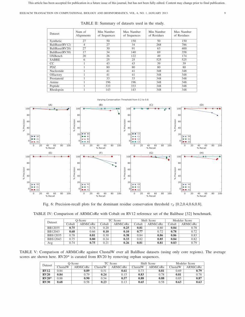
C. Effects of Important Thresholds

The parameters that have the most significant impact on

the number of coupled patterns discovered are the dominant

residue conservation threshold (τd ), block coverage threshold

(τ ), and column-window size threshold (ε). Based on the

27 synthetic alignments, we produced precision-recall curves

using various values for τd, τ and ε. In synthetic alignments

couplings are embedded. We run our methods on these datasets

to discover coupled patterns based on various parameters and

see how many of the discovered coupled patterns are matched

(true positive) and how many are redundant (false positive).

The precision-recall curve for τd ∈ {0.2, 0.4, 0.6, 0.8} which

are illustrated in Fig. 6. We vary the block pattern threshold

parameter τ in the set {0.4, 0.6, 0.8, 0.10, 0.12} and generate

precision-recall plots (Fig. not shown). Similarly, we produce

precision-recall curves for ε ∈ {1, 2, 3, 4, 5} (Fig. not shown).

As all the plots reveal, our method maintain consistently high

levels of recall and precision across a wide range of thresholds.

D. Comparison with ClustalW and COBALT

We evaluate ARMiCoRe on all the datasets described ear-

lier: synthetic, benchmark and alignments with couplings. For

each of these alignments, we remove gaps and realign with

ClustalW in default settings (using the PAM matrix). We

then run ARMiCoRe on each of the ClustalW alignments

to generate coupled patterns and use the coupled patterns to

generate constraints, which are used by COBALT to create

an improved alignment. We then compare our scores with

ClustalW and with COBALT (without any constraints input).

As shown in Table III ARMiCoRe excels in all four

traditional measures of MSA quality for synthetic datasets.



TABLE II: Summary of datasets used in the study.

DatasetNum ofAlignments

Min Numberof Sequences

Max Numberof Sequences

Min Numberof Residues

Max Numberof Residues

Synthetic 27 50 150 50 150BaliBase(RV12) 4 27 34 268 786BaliBase(RV20) 27 30 91 63 400BaliBase(RV30) 17 34 140 69 358OXBench 20 26 122 49 174SABRE 6 25 25 525 525CC 1 43 43 39 39PDZ 1 80 80 80 80Nucleotide 1 41 41 348 348Olfactory 1 41 41 348 348Prostanoid 1 33 33 348 348Amine 1 196 196 348 348Peptide 1 333 333 348 348Rhodopsin 1 143 143 348 348

0 20 40 60 80 100% Recall

0

20

40

60

80

100

% P

recis

ion

(A)

A0

A1

A2

0 20 40 60 80 100% Recall

0

20

40

60

80

100

% P

recis

ion

(B)

B0

B1

B2

B3

0 20 40 60 80 100% Recall

0

20

40

60

80

100

% P

recis

ion

(C)

C0

C1

C2

C3

0 20 40 60 80 100% Recall

0

20

40

60

80

100

% P

recis

ion

(D)

D0

D1

D2

0 20 40 60 80 100% Recall

0

20

40

60

80

100

% P

recis

ion

(E)

E0

E1

E2

0 20 40 60 80 100% Recall

0

20

40

60

80

100

% P

recis

ion

(F)

F0

F1

F2

0 20 40 60 80 100% Recall

0

20

40

60

80

100

% P

recis

ion

(G)

G0

G1

G2

0 20 40 60 80 100% Recall

0

20

40

60

80

100

% P

recis

ion

(H)

H0

H1

H2

Varying Conservation Threshold from 0.2 to 0.8

Fig. 6: Precision-recall plots for the dominant residue conservation threshold τd [0.2,0.4,0.6,0.8].

TABLE IV: Comparison of ARMiCoRe with Cobalt on RV12 reference set of the Balibase [32] benchmark.

DatasetQ-Score TC Score Shift Score Modeler Score

Cobalt ARMiCoRe Cobalt ARMiCoRe Cobalt ARMiCoRe Cobalt ARMiCoReBB12035 0.75 0.74 0.20 0.25 0.81 0.80 0.84 0.78BB12043 0.68 0.66 0.10 0.10 0.77 0.72 0.78 0.72BBS12035 0.78 0.81 0.30 0.38 0.84 0.86 0.86 0.83BBS12043 0.75 0.80 0.24 0.33 0.82 0.85 0.84 0.82Avg 0.74 0.75 0.21 0.26 0.81 0.81 0.83 0.79

TABLE V: Comparison of ARMiCoRe against ClustalW over all BaliBase datasets (using only core regions). The average

scores are shown here. RV20* is curated from RV20 by removing orphan sequences.

DatasetQ-Score TC Score Shift Score Modeler Score

ClustalW ARMiCoRe ClustalW ARMiCoRe ClustalW ARMiCoRe ClustalW ARMiCoReRV12 0.84 0.89 0.51 0.61 0.73 0.81 0.69 0.79RV20 0.84 0.79 0.24 0.15 0.83 0.78 0.81 0.78RV20* 0.88 0.90 0.54 0.57 0.88 0.88 0.85 0.87RV30 0.68 0.58 0.23 0.13 0.65 0.58 0.63 0.63



TABLE VI: Comparison of ARMiCoRe against ClustalW and

COBALT over OXBench alignments.

Dataset Score ClustalW COBALT ARMiCoRe

12s107

Q-Score 0.99 0.99 0.98TC Score 0.80 0.93 0.86Shift Score 0.93 0.93 0.92Modeler Score 0.87 0.87 0.87

12s108


12t109


12t113


12t116


.

.

....

.

.

....

.

.

.

588t28


22s38


22t50


588


12


Table IV depicts the superior performance of ARMiCoRe

over COBALT on three of the four measures in the RV12

reference set of the BaliBase benchmark. Performance of

ARMiCoRe against ClustalW on all reference sets of the

BaliBase benchmark is given in Table V. ARMiCoRe shows

superior performance over ClustalW on all of the four mea-

sures in the RV12 reference set. The sequence identity in

this benchmark is about 20–40%. Note that the performance

of ARMiCoRe on RV20 and RV30 is worse than that of

ClustalW in all four measures. This is because RV20 and RV30

pool together sequences with poor similarity and thus coupled

patterns are not a driver for obtaining good alignments. The

effect of an orphan sequence on the similarity structure of

an alignment is illustrated in Fig. 7. To test this hypothesis,

we removed the orphan sequences from RV20 (RV20*) and

as Table V shows, the performance of ARMiCoRe is better

along three of the four measures. Table VI describes the

results of ARMiCoRe for the OXBench benchmark, once

again revealing a mixed performance on a dataset with high

sequence diversity. Finally, Table VII depicts the superior per-

TABLE VII: Comparison of ARMiCoRe against ClustalW and

COBALT over SABRE alignments.


sup 038

Q-Score 0.82 0.83 0.88TC Score 0 0 0Shift Score 0.17 0.18 0.19Modeler Score 0.10 0.10 0.12

sup 092


sup 108

Q-Score 0.89 0.92 0.93TC Score 0 0.35 0.35Shift Score 0.46 0.48 0.48Modeler Score 0.31 0.32 0.32

sup 126

Q-Score 0.51 0.76 0.59TC Score 0 0.14 0Shift Score 0.19 0.30 0.23Modeler Score 0.12 0.18 0.14

sup 167


sup 215


TABLE VIII: Comparison of ARMiCoRe against ClustalW

and COBALT over CC subfamily of WW protein family, PDZ

family, and Nucleotide subfamily of GPCR family.


CC

Q-Score 0.89 0.85 0.96TC Score 0.51 0.35 0.51Shift Score 0.93 0.91 0.97Modeler Score 0.90 0.91 0.97C-Score 0.71 0.88 1.00

PDZ

Q-Score 0.85 0.82 0.87TC Score 0 0.1 0Shift Score 0.89 0.87 0.9Modeler Score 0.85 0.89 0.88C-Score 0.67 0.81 0.81

Nucleotide

Q-Score 0.74 0.68 0.79TC Score 0.46 0.34 0.45Shift Score 0.79 0.74 0.83Modeler Score 0.74 0.77 0.80C-Score 0.52 0.50 0.63

formance of ARMiCoRe over ClustalW in 5 alignments out of

6 alignments in SABRE dataset. In Tables VI and VII, we see

that sometimes ARMiCoRe performs relatively poor compare

to COBALT. The reason might be the sequence similarity

structure of the alignments or poor choice of gap penalties

for realignment. Note that these benchmark datasets are not

designed for evaluating couplings’ discovery algorithms in

protein families.

E. Modeling Correlated Mutations

We describe the effect of ARMiCoRe on three families

that are known to exhibit correlated mutations. We focus on

the CC subfamily of the WW domain, the PDZ family, and

the Nucleotide subfamily of the GPCR family. Based on C-

Score, we evaluate the Performance of ARMiCoRe against

ClustalW and COBALT. As shown in Table VIII, ARMiCoRe

is consistently better on at least three measures.



0.1 0.2 0.3 0.4 0.5 0.6 0.7 0.80

50

100

150

200

250

300

Pairwise SeqID

Cou

nt

0.2 0.25 0.3 0.35 0.4 0.45 0.5 0.55 0.6 0.650

50

100

150

200

250

300

Pairwise SeqID

Cou

nt

(a) (b)Fig. 7: Pairwise sequence similarity analysis of an alignment ‘BB20006’ from RV20 dataset that contains an orphan sequence.

We use SCA [39] for this analysis. Fig. 7a has a peak for similarity score around 0.12 that indicates that the orphan is distant

from the other sequences. Fig. 7b shows a reasonably narrow distribution without the orphan sequence with a mean pairwise

similarity between sequences of about 27% and a range of 20% to 35%, which suggests that most sequences are about equally

dissimilar from other.

Fig. 9: Interfaces for mining coupled patterns. (a) Loading of An input alignment. (b) Selection of coupled patterns with

colored plot of corresponding residues.

Fig. 8: An overview of user interaction with ARMiCoRe.

F. Evaluation using Global Statistical Model for ResidueCouplings

Couplings are often employed to predict 3D structure of

proteins from sequences. A global statistical method for

residue couplings for predicting 3D structure of proteins is

proposed by Marks et al. [40]. The proposed method first

calculates pairwise coupling scores and then uses high scoring

pairs to find a 3D structure. The way of calculating couplings

scores is global which is different from the method given by

Thomas et al. [38]. We use their method to calculate pairwise

couplings scores for reference, ClustalW, and ARMiCoRe

alignments. We then identify how many of the coupled pairs

(true positive) for the reference alignment are also retained in

ClustalW and ARMiCoRe alignments for various thresholds.

In Table IX and Table XI we see that the alignments for CC

and Nucleotide subfamily given by ARMiCoRe is much better

than that of ClustalW. But the alignment for PDZ family given

by ARMiCoRe is not better than that of ClustalW in terms

of couplings calculated in global settings (see Table X). The

scores produced by ARMiCoRe are low for both PDZ and

Nucleotide families. To get an insight we perform sequence

similarity analysis using SCA tool [39]. We have seen wider

distributions of sequence similarities with multiple peaks for

PDZ and Nucleotide families which indicates that sequences

are not equally dissimilar from each other and the presence of

subclusters of sequences within the family.



TABLE IX: Comparison of ARMiCoRe against ClustalW over the CC subfamily of WW family using the global residue

coupling model defined in [40]. Here ‘TP’ is used for true positive, ‘P’ is used for precision, and ‘R’ is used for recall.

ScoreThreshold

Number ofcouplings inRef MSA

Number ofcouplings inClustalW MSA

TP P RF1Score

Num of couplingsin ARMiCoReMSA

TP P RF1Score

0.40 8 5 1 0.20 0.13 0.15 5 3 0.60 0.38 0.460.35 27 19 13 0.68 0.48 0.57 29 21 0.72 0.78 0.750.30 64 51 36 0.71 0.56 0.63 61 53 0.87 0.83 0.85

TABLE X: Comparison of ARMiCoRe against ClustalW over the PDZ family using the global residue coupling model defined

in [40]. Here ‘TP’ is used for true positive, ‘P’ is used for precision, and ‘R’ is used for recall.

ScoreThreshold



TP P RF1Score


TP P RF1Score

0.20 15 13 4 0.27 0.31 0.29 17 3 0.20 0.18 0.190.15 64 71 21 0.33 0.30 0.31 82 13 0.20 0.16 0.180.10 396 405 190 0.48 0.47 0.47 474 145 0.37 0.31 0.33

TABLE XI: Comparison of ARMiCoRe against ClustalW over the Nucleotide subfamily of GPCR family using the global

residue coupling model defined in [40]. Here ‘TP’ is used for true positive, ‘P’ is used for precision, and ‘R’ is used for recall.

ScoreThreshold



TP P RF1Score


TP P RF1Score

0.15 7 7 0 0.00 0.00 - 9 1 0.11 0.14 0.130.12 14 14 1 0.07 0.07 0.07 24 3 0.13 0.21 0.160.10 21 23 2 0.09 0.10 0.09 37 5 0.14 0.24 0.17

0.1 0.15 0.2 0.25 0.3 0.35 0.4 0.45 0.5 0.55 0.60

20

40

60

80

100

120

Pairwise SeqID

Cou

nt

0 0.1 0.2 0.3 0.4 0.5 0.6 0.70

20

40

60

80

100

120

Pairwise SeqID

Cou

nt

0.1 0.15 0.2 0.25 0.3 0.35 0.4 0.45 0.5 0.55 0.60

20

40

60

80

100

120

Pairwise SeqID

Cou

nt

(a) (b) (c)

Fig. 10: Pairwise sequence similarity analysis using SCA [39]. Histograms for reference, ClustalW, and ARMiCoRe are drawn

for the same number of bins. This figure shows that the ARMiCoRe alignment retains most of the sequence similarity structure

of the reference alignment.

TABLE XII: Comparison of ARMiCoRe against ClustalW over the CC subfamily of WW family using the statistical coupling

analysis defined in [41]. Here ‘TP’ is used for true positive, ’P’ is used for precision, and ’R’ is used for recall.

Cut-offThreshold

Sector Sizein Ref MSA

Sector Size inClustalW MSA

TP P RF1Score

Sector Size inARMiCoRe MSA

TP P RF1Score

0.85 7 5 5 1.00 0.71 0.83 7 6 0.86 0.86 0.860.80 11 7 7 1.00 0.64 0.78 9 9 1.00 0.82 0.900.75 12 8 8 1.00 0.67 0.80 12 11 0.92 0.92 0.92

G. Evaluation using Statistical Coupling Analysis

Lockless and Ranganathan [41] proposed statistical cou-

pling analysis (SCA) as a method for analyzing coevolution

in protein families represented by MSAs. The SCA tool [39]

performs sequence similarity analysis to get an idea of the

number of subfamilies in the MSA. We perform similarity

analysis for the reference, ClustalW, and ARMiCoRe align-

ments of CC family (see Fig. 10). There are two subfamilies

for the CC family: folded and non-folded. Fig. 10 shows that

for both reference and ARMiCoRe alignments there are two

peaks in the histogram which is an indication that there are two

subfamilies, whereas the ClustalW alignment indicates that the

similarity structure for two subfamilies are distorted.

SCA also allows us to identify protein sectors, which are

quasi-independent groups of correlated amino acids [42]. We

identify protein sectors of reference, ClustalW, and ARMi-

CoRe alignments for various cut-off thresholds (0.85, 0.80,

and 0.75). We then calculate precision, recall, and F1-score



TABLE XIII: Comparison of ARMiCoRe with ClustalW and

COBALT using avergare runtime per alignment. Times are

given in seconds.

Dataset ClustalW COBALT ARMiCoRe

BaliBase 3.2 1.74 5.23OXBench 2.76 2.18 4.77SABRE 0.80 3.41 3.53

for ClustalW and ARMiCoRe alignments with respect to the

reference alignment. For all of the cut-off thresholds one

protein sector is identified. Table XII shows that much of

protein sector in the reference alignment is retained in the

ARMiCoRe alignment.

H. User Interaction in Choosing Couplings

We have developed GUIs for ARMiCoRe that allow users to

interactively choose patterns from a set of significant coupled

patterns and use them to realign sequences. This enables

biologists to bring specific domain knowledge in deciding

which coupled pattern sets should be exposed as couplings

in the new alignment. We have integrated ARMiCoRe with

the JalView [43] framework, which has a rich set of sequence

analysis tools. A typical workflow with ARMiCoRe is illus-

trated in Fig. 8. A user begins an experiment by loading an

initial alignment (see Fig. 9(a)). He or she can evaluate the

input alignment by measuring various scores with respect to a

reference alignment. Based on the evaluation, he or she may

decide to improve the alignment using the coupled pattern

mining module. The coupled pattern mining module facilitates

tuning various parameters prior to the pattern mining and gives

a set of significant coupled patterns as output. From the pool

of coupled patterns, a domain expert can choose meaningful

patterns (see Fig. 9(b)) and use them in the realignment

module. The realignment module gives a new alignment,

which can be evaluated in the evaluation module. A user may

repeat the realignment step by choosing different patterns or

the mining step by tuning the parameters.

I. Experimental Runtime

We compare ARMiCoRe against ClustalW and COBALT

based on experimental runtime on three benchmark datasets:

BaliBase, OXBench, and SABRE (see Table XIII). As ex-

pected ARMiCoRe takes more time than ClustalW and

COBALT but the runtime of ARMiCoRe is reasonable.

VI. DISCUSSION

Evolutionary constraints on genes and proteins to main-

tain structure and function are revealed as conservation and

coupling in an MSA. The advent of cheap, high-throughput

sequencing promises to provide a wealth of sequence data

enabling such applications, but at the same time requires

methods such as ARMiCoRe to improve the alignments and

inferred constraints upon which they are based. The alignments

obtained by ARMiCoRe can be leveraged to design or classify

novel proteins that are stably folded and functional [44], [45],

[41], as well as to predict three-dimensional structures from

sequence alone [40], [46]. Our work also demonstrates a

successful application of pattern set mining where the goal

is not just to find patterns but to cover the set of sequences

with discovered patterns such that an objective measure is

optimized. The ideas developed here can be generalized to

other pattern set mining problems in areas like neuroscience,

sustainability, and systems biology.

ACKNOWLEDGEMENT

This work is supported in part by US NSF grant IIS-

0905313.

REFERENCES

[1] T. Hubbard, A. Lesk, and A. Tramontano, “Gathering Them in to theFold,” Nat. Struct. Mol. Biol., vol. 3, no. 4, p. 313, 1996.

[2] J. Thompson, D. Higgins, and T. Gibson, “CLUSTAL W: Improvingthe Sensitivity of Progressive Multiple Sequence Alignment throughSequence Weighting, Position-specific Gap Penalties and Weight MatrixChoice,” Nucleic Acids Res., vol. 22, pp. 4673–4680, 1994.

[3] A. Loytynoja and M. Milinkovitch, “A Hidden Markov Model forProgressive Multiple Alignment,” Bioinformatics, vol. 19, no. 12, pp.1505–1513, 2003.

[4] R. Edgar, “MUSCLE: Multiple Sequence Alignment with High Accu-racy and High Throughput,” Nucleic Acids Res., vol. 32, pp. 1792–1797,2004.

[5] C. Notredame, D. Higgins, and J. Heringa, “T-coffee: A Novel Methodfor Fast and Accurate Multiple Sequence Alignment,” J. Mol. Biol., vol.302, no. 1, pp. 205–217, 2000.

[6] B. Bringmann, S. Nijssen, N. Tatti, J. Vreeken, and A. Zimmermann.Mining Sets of Patterns: A Tutorial at ECMLPKDD 2010, Barcelona,Spain. [Online]. Available: http://www.cs.kuleuven.be/conference/msop/

[7] R. Edgar and S. Batzoglou, “Multiple Sequence Alignment,” Curr. Opin.Struct. Biol., vol. 16, no. 3, pp. 368–373, 2006.

[8] C. Do and K. Katoh, “Protein Multiple Sequence Alignment,” inFunctional Proteomics, 2008, vol. 484, ch. 25, pp. 379–413.

[9] K. Katoh, K. Misawa, K. Kuma, and T. Miyata, “MAFFT: A NovelMethod for Rapid Multiple Sequence Alignment Based on Fast FourierTransform,” Nucleic Acids Res., vol. 30, no. 14, pp. 3059–3066, 2002.

[10] C. Do, M. Mahabhashyam, M. Brudno, and S. Batzoglou, “ProbCons:Probabilistic Consistency-based Multiple Sequence Alignment,” GenomeRes., vol. 15, pp. 330–340, 2005.

[11] B. Morgenstern, “DIALIGN: Multiple DNA and Protein SequenceAlignment at BiBiServ,” Nucleic Acids Res., vol. 32, no. suppl 2, pp.W33–W36, 2004.

[12] A. Subramanian, J. Weyer-Menkhoff, M. Kaufmann, and B. Mor-genstern, “DIALIGN-T: An Improved Algorithm for Segment-basedMultiple Sequence Alignment,” BMC Bioinformatics, vol. 6, no. 1, p. 66,2005.

[13] C. Lee, C. Grasso, and M. Sharlow, “Multiple Sequence Alignment usingPartial Order Graphs,” Bioinformatics, vol. 18, no. 3, pp. 452–464, 2002.

[14] H. Carrillo and D. Lipman, “The Multiple Sequence Alignment Problemin Biology,” SIAM J. Appl. Math., vol. 48, no. 5, pp. 1073–1082, 1988.

[15] L. Wang and T. Jiang, “On the Complexity of Multiple SequenceAlignment,” J. Comp. Biol., vol. 1, no. 4, pp. 337–348, 1994.

[16] M. Brudno, C. B. Do, G. M. Cooper, M. F. Kim, E. Davydov, E. D.Green, A. Sidow, S. Batzoglou et al., “LAGAN and Multi-LAGAN:Efficient Tools for Large-Scale Multiple Alignment of Genomic DNA,”Genome Res., vol. 13, no. 4, pp. 721–731, 2003.

[17] S. Yamada, O. Gotoh, and H. Yamana, “Improvement in Accuracy ofMultiple Sequence Alignment using Novel Group-to-group SequenceAlignment Algorithm with Piecewise Linear Gap Cost,” BMC Bioinfor-matics, vol. 7, no. 1, p. 524, 2006.

[18] O. Gotoh, “Significant Improvement in Accuracy of Multiple ProteinSequence Alignments by Iterative Refinement as Assessed by Referenceto Structural Alignments,” J. Mol. Biol., vol. 264, no. 4, pp. 823–838,1996.

[19] W. Bains, “MULTAN: A Program to Align Multiple DNA Sequences,”Nucleic Acids Res., vol. 14, no. 1, pp. 159–177, 1986.

[20] J. Pei and N. Grishin, “PROMALS: Towards Accurate Multiple Se-quence Alignments of Distantly Related Proteins,” Bioinformatics,vol. 23, no. 7, pp. 802–808, 2007.



[21] J. Pei, R. Sadreyev, and N. Grishin, “PCMA: Fast and Accurate MultipleSequence Alignment Based on Profile Consistency,” Bioinformatics,vol. 19, no. 3, pp. 427–428, 2003.

[22] J. Papadopoulos and R. Agarwala, “COBALT: Constraint-based Align-ment Tool for Multiple Protein Sequences,” Bioinformatics, vol. 23,no. 9, pp. 1073–1079, 2007.

[23] J. D. Thompson, F. Plewniak, J. Thierry, and O. Poch, “DbClustal: Rapidand Reliable Global Multiple Alignments of Protein Sequences Detectedby Database Searches,” Nucleic Acids Res., vol. 28, no. 15, pp. 2919–2926, 2000.

[24] L. Guasco, “Multiple Sequence Alignment Correction using Con-straints,” Ph.D. dissertation, Universidade Nova de Lisboa, 2010.

[25] R. Gouveia-Oliveira and A. Pedersen, “Finding Coevolving Amino AcidResidues using Row and Column Weighting of Mutual Informationand Multi-dimensional Amino Acid Representation,” Algorithms forMolecular Biology, vol. 1, p. 12, 2007.

[26] R. Agrawal, H. Mannila, R. Srikant, H. Toivonen, and A. Verkamo, “Fastdiscovery of association rules,” Advances in Knowledge Discovery andData Mining, pp. 307–328, 1996.

[27] W. Taylor, “The Classification of Amino Acid Conservation,” J. Theor.Biol., vol. 119, pp. 205–218, 1986.

[28] G. Nemhauser, L. Wolsey, and M. Fisher, “An Analysis of Approxima-tions for Maximizing Submodular Set Functions-I,” Math. Prog., vol. 14,pp. 265–294, 1978.

[29] J. Edmonds and R. M. Karp, “Theoretical Improvements in AlgorithmicEfficiency for Network Flow Problems,” J. ACM, vol. 19, pp. 248–264,April 1972.

[30] A. Goldberg and R. Tarjan, “A New Approach to the Maximum-FlowProblem,” J. ACM, vol. 35, pp. 921–940, 1988.

[31] B. Morgenstern, K. Frech, A. Dress, and T. Werner, “DIALIGN: FindingLocal Similarities by Multiple Sequence Aalignment,” Bioinformatics,vol. 14, no. 3, pp. 290–294, 1998.

[32] J. Thompson, P. Koehl, R. Ripp, and O. Poch, “BAliBASE 3.0: Lat-est Developments of the Multiple Sequence Alignment Benchmark,”Proteins: Structure, Function, and Bioinformatics, vol. 61, no. 1, pp.127–136, 2005.

[33] G. P. S. Raghava, S. Searle, P. Audley, J. Barber, and G. Barton,“OXBench: A Benchmark for Evaluation of Protein Multiple SequenceAlignment Accuracy,” BMC bioinformatics, vol. 4, no. 1, p. 47, 2003.

[34] R. Edgar, “MSA Benchmark Collection,” Available at http://www.drive5.com/bench/.

[35] W. K. Kroeze, D. J. Sheffler, and B. L. Roth, “G-protein-coupledReceptors at a Glance,” J. Cell Sci., vol. 116, pp. 4867–4869, 2003.

[36] J. Sauder, J. Arthur, and R. Dunbrack, “Large-scale Comparison ofProtein Sequence Alignment Algorithms with Structure Alignments,”Proteins, vol. 40, pp. 6–22, 2000.

[37] M. Cline, R. Hughey, and K. Karplus, “Predicting Reliable Regions inProtein Sequence Alignments,” Bioinformatics, vol. 18, no. 2, pp. 306–314, 2002.

[38] J. Thomas, N. Ramakrishnan, and C. Bailey-Kellogg, “Graphical Modelsof Residue Coupling in Protein Families,” IEEE/ACM Transactions onComputational Biology and Bioinformatics, vol. 5, no. 2, pp. 183–197,2008.

[39] R. Ranganathan, “Statistical Coupling Analysis,” Available at http://systems.swmed.edu/rr lab/sca.html.

[40] D. Marks, L. Colwell, R. Sheridan, T. Hopf, A. Pagnani, R. Zecchina,and C. Sander, “Protein 3D Structure Computed from EvolutionarySequence Variation,” PLoS ONE, vol. 6, no. 12, p. e28766, 2011.

[41] S. W. Lockless and R. Ranganathan, “Evolutionarily Conserved Path-ways of Energetic Connectivity in Protein Families,” Science, vol. 286,no. 5438, pp. 295–299, 1999.

[42] N. Halabi, O. Rivoire, S. Leibler, and R. Ranganathan, “Protein Sectors:Evolutionary Units of Three-Dimensional Structure,” Cell, vol. 138, pp.774–786, 2009.

[43] A. Waterhouse, J. Procter, D. Martin, M. Clamp, and G. Barton, “JalviewVersion 2 – A Multiple Sequence Alignment Editor and AanalysisWorkbench,” Bioinformatics, vol. 25, no. 9, pp. 1189–1191, 2009.

[44] S. Balakrishnan, H. Kamisetty, J. Carbonell, S. Lee, and C. Langmead,“Learning Generative Models for Protein Fold Families,” Proteins:Structure, Function, and Bioinformatics, vol. 79, no. 4, pp. 1061–1078,2011.

[45] J. Thomas, N. Ramakrishnan, and C. Bailey-Kellogg, “Protein Designby Sampling an Undirected Graphical Model of Residue Constraints,”IEEE/ACM Transactions on Computational Biology and Bioinformatics,vol. 6, no. 3, pp. 506–516, 2009.

[46] T. Hopf, L. Colwell, R. Sheridan, B. Rost, C. Sander, and D. Marks,“Three-Dimensional Structures of Membrane Proteins from GenomicSequencing,” Cell, vol. 149, no. 7, pp. 1607–1621, 2012.

K. S. M. Tozammel Hossain is pursuing Ph.D.degree in computer science at Virginia Tech. Heholds a B.S. in computer science & engineeringfrom Bangladesh University of Engineering & Tech-nology. His current research interests are in bioin-formatics, in particular identifying and modelingevolutionary constraints to assist in protein analysis,classification, and design.

Debprakash Patnaik is currently an engineer inthe Search and Discovery group at Amazon.com.He completed his Ph.D. in Computer Science fromVirginia Tech, USA. He received his bachelor degreefrom Veer Surendra Sai University of Technology,Orissa, India, in 2002 and masters degree fromIndian Institute of Science, Bangalore, in 2006.He also worked as a researcher in the Diagnosisand Prognosis group at General Motors Research,Bangalore. His research interests include temporaldata mining, probabilistic graphical models, and

application in neuroscience.

Srivatsan Laxman is a researcher at MicrosoftResearch India, Bangalore and is associated with tworesearch areas, Machine Learning & Optimizationand Security & Privacy. He works broadly in datamining, machine learning and data privacy. Srivatsanreceived his PhD in Electrical Engineering in 2006from Indian Institute of Science, Bangalore.

Prateek Jain is a researcher in the Machine Learn-ing and Optimization group at Microsoft Research,Bangalore, India. His research interests lie in theareas of machine learning, optimization, and high-dimensional statistics. Before joining Microsoft, Pra-teek obtained his Ph.D. from the CS departmentat the University of Texas at Austin. He and hiscollaborators were recognized with the ICML BestStudent Paper Award in 2007, SDM Best PaperRunner-up Award in 2008, and with the CVPR BestStudent Paper Award in 2008.

Chris Bailey-Kellogg is an associate professor ofcomputer science at Dartmouth. He earned a BS/MSwith Sandy Pentland at MIT and a PhD with FengZhao at Ohio State and Xerox PARC, and conductedpostdoctoral research with Bruce Donald at Dart-mouth. He was an assistant professor at Purdue be-fore being recruited back to Dartmouth. His researchfocuses on integrating computation and experimentin studies of protein structure and function, with aparticular emphasis on applications to protein andvaccine design.

Naren Ramakrishnan is the Thomas L. PhillipsProfessor of Engineering at Virginia Tech and di-rector of the university’s Discovery Analytics Center(DAC; http://dac.cs.vt.edu). His research interestsinvolve mining scientific datasets, in domains suchas intelligence analysis, sustainability, neuroscience,and systems biology. Ramakrishnan’s work has beensupported by NSF, DHS, NIH, NEH, DARPA,IARPA, ONR, General Motors, HP Labs, NEC Labs,and Advance Auto Parts. He received his PhD inComputer Sciences from Purdue University.


Documents

Improved Multiple Sequence Alignments Using Coupled Pattern Mining