Implicit weighted essentially non-oscillatory schemes … · IMPLICIT WEIGHTED ESSENTIALLY NON-OSCILLATORY SCHEMES FOR THE ... for compressible flows, ... In order to apply compressible

INTERNATIONAL JOURNAL FOR NUMERICAL METHODS IN FLUIDS

Int. J. Numer. Meth. Fluids 31: 747–765 (1999)

IMPLICIT WEIGHTED ESSENTIALLYNON-OSCILLATORY SCHEMES FOR THE

INCOMPRESSIBLE NAVIER–STOKES EQUATIONS

YIH-NAN CHENa, SHIH-CHANG YANGa AND JAW-YEN YANGb,*a Department of Mechanical Engineering, National Taiwan Uni6ersity, Taipei, Taiwan, Republic of China

b Institute of Applied Mechanics, National Taiwan Uni6ersity, Taipei, Taiwan, Republic of China

SUMMARY

A class of lower–upper/approximate factorization (LUAF) implicit weighted essentially non-oscillatory(ENO; WENO) schemes for solving the two-dimensional incompressible Navier–Stokes equations in ageneralized co-ordinate system is presented. The algorithm is based on the artificial compressibilityformulation, and symmetric Gauss–Seidel relaxation is used for computing steady state solutions whilesymmetric successive overrelaxation is used for treating time-dependent flows. WENO spatial operatorsare employed for inviscid fluxes and central differencing for viscous fluxes. Internal and external viscousflow test problems are presented to verify the numerical schemes. The use of a WENO spatial operatornot only enhances the accuracy of solutions but also improves the convergence rate for the steady statecomputation as compared with using the ENO counterpart. It is found that the present solutionscompare well with exact solutions, experimental data and other numerical results. Copyright © 1999John Wiley & Sons, Ltd.

KEY WORDS: WENO schemes; artificial compressibility; incompressible; Navier–Stokes equations

1. INTRODUCTION

The design and construction of the weighted essentially non-oscillatory (WENO) schemes forhyperbolic conservation laws are based on essentially non-oscillatory (ENO) schemes that werefirst introduced by Harten et al. [1] in the form of cell averages. Later, to improve theimplementation of the method, Shu and Osher [2,3] devised a class of flux-based efficient ENOschemes. The main concept of ENO schemes is to use the ‘smoothest’ stencil (in the asymptoticsense) among several candidates to approximate the fluxes at cell boundaries to a high-orderaccuracy, and at the same time, to avoid oscillations near discontinuities. ENO schemes areuniformly high-order accurate right up to the shock and are very robust to use. However, theyalso have certain drawbacks as Jiang and Shu [4] have pointed out. One problem is that thefreely adaptive stencil could change even by a round-off perturbation near zeroes of thesolution and its derivatives. This free adaptation of the stencil is also not necessary in regionswhere the solution is smooth. The convergence rate for the implicit ENO scheme is generallypoor. Another problem is that ENO schemes are not effective on vector supercomputersbecause the stencil-choosing step involves heavy usage of logical statement, which performs

* Correspondence to: Institute of Applied Mechanics, College of Engineering, National Taiwan University, Taipei10764, Taiwan, Republic of China.

CCC 0271–2091/99/200747–19$17.50Copyright © 1999 John Wiley & Sons, Ltd.

Recei6ed August 1997Re6ised July 1998

Y.-N. CHEN ET AL.748

poorly on such machines. The WENO schemes proposed recently by Jiang and Shu [4] andby Liu et al. [5] can overcome these drawbacks while keeping the robustness and high-orderaccuracy of ENO schemes. The concept of WENO schemes is the following: instead ofapproximating the numerical flux using only one of the candidate stencils, one uses aconvex combination of all the candidate stencils. Each of the candidate stencils is assigneda weight which determines the contribution of this stencil to the final approximation of thenumerical flux. The weights are defined in such a way that, in smooth regions, it ap-proaches certain optimal weights to achieve a higher order of accuracy, while in regionsnear discontinuities, the stencils that contain the discontinuities are assigned a nearly zeroweight. Thus, ENO property is achieved by emulating ENO schemes around discontinuitiesand a higher order of accuracy is obtained by emulating upstream central schemes with theoptimal weights away from the discontinuities. Both efficient ENO and WENO schemeshave been extensively tested and applied to the compressible Euler/Navier–Stokes equa-tions.

The solution methodology for viscous incompressible flows is rather different from thatfor compressible flows, due to the fact that there exists no time derivative in the continuityequation for incompressible flows. In order to apply compressible flow solution algorithmsto incompressible flow problems, the continuity equation needs to be modified to couplewith the momentum equation so that the whole system of equations can be put into thesame formulation and solved efficiently. To achieve this goal, the artificial compressibilitymay be introduced by adding the time derivative of pressure to the continuity equation, aswas first proposed by Chorin [6]. The modified continuity equation, together with theunsteady momentum equations, yield a set of hyperbolic–parabolic type of time-dependentsystem of equations. Thus, fast implicit schemes developed for compressible flows, such asthe approximate-factorization scheme by Beam and Warming [7], can be implemented.Various applications that evolved from this artificial compressibility concept have beenreported for obtaining steady state solutions [8–14]. Merkle and Athavale [15] and Rogersand Kwak [16,17] have reported successful computations using the pseudo-time iterationapproach for the time-dependent flow problems. Further developments of numerical meth-ods for incompressible viscous flows can be found in the work by Anderson et al. [18] andby Briley et al. [19].

In this paper, the WENO scheme of Jiang and Shu [4] is adopted and is extended tosolve the incompressible flow problems. An implicit code of the WENO scheme is devel-oped for the artificial compressibility formulation of the two-dimensional incompressibleNavier–Stokes equations for both steady state and time-dependent flows. For the steadystate flow problems, the lower–upper symmetric-Gauss–Seidel (LU-SGS) implicit algorithm[20] is adopted. This algorithm is not only unconditionally stable but also completelyvectorizable in any dimension. For the time-dependent flow problems, the lower–uppersymmetric successive overrelaxation (LU-SSOR) scheme [21] is employed. For saving CPUtime, the pseudo-time iteration approach was not used. Instead, the values of b have beenput in the range b]5 (i.e. the larger the b value, the minor the influence of the timederivative term in the continuity equation becomes). The resulting schemes are applied tocompute several standard internal and external laminar flow problems, including drivensquare cavity flow, flow over a backward-facing step, flow decayed by viscosity and flowover a circular cylinder. It is found that the present solutions are in good agreement withavailable experimental results, exact solutions and other numerical results.

Copyright © 1999 John Wiley & Sons, Ltd. Int. J. Numer. Meth. Fluids 31: 747–765 (1999)

2D INCOMPRESSIBLE NAVIER–STOKES EQUATIONS 749

2. GOVERNING EQUATIONS

The Navier–Stokes equations in the integral conservation law form for an incompressible,two-dimensional flow with artificial compressibility can be written as

(

(t�1

V&

V

Q dV�

+1V7

S

Fa ·dSa =0, (1)

where V is the volume of the arbitrary control volume, S is the area of the arbitrary controlsurface and the direction of dSa is outward, Q is the vector form of the conservative variablesand Fa = (E−E6)ib + (F−F6)jb is the flux tensor. In a Cartesian co-ordinates system, Equation(1) can be expressed as follows:

(Q(t

+((E−E6)(x

+((F−F6)(y

=0, (2)

with

Q=ÃÆ

È

pu6

ÃÇ

É, E=Ã

Æ

È

buu2+p

u6ÃÇ

É, F=Ã

Æ

È

b6

6u62+p

ÃÇ

É,

E6=Re−1ÃÆ

È

02ux

uy+6x

ÃÇ

É, F6=Re−1Ã

Æ

È

06x+uy

26y

ÃÇ

É,

where b is the artificial compressibility parameter and Re=rV�L/m is the Reynolds number.The Cartesian velocity components u and 6 are scaled with the freestream velocity V� and theCartesian co-ordinates x and y are normalized with the characteristic length L. The non-dimensional pressure is defined as p= (P−P�)/rV�2 , and the dynamic viscosity m is assumedto be constant.

Conventionally, Equation (2) is transformed into the generalized co-ordinates (j, h) as

(Q.(t

+((E. −E. 6)(j

+((F. −F. 6)(h

=0, (3)

where

Q. =hÃÆ

È

pu6

ÃÇ

É, E. =hÃ

Æ

È

bUuU+jxp6U+jyp

ÃÇ

É, F. =hÃ

Æ

È

bVuV+hxp6V+hyp

ÃÇ

É,

E. 6=h [jxE6+jyF6 ], F. 6=h [hxE6+hyF6 ]

and

U=jxu+jy6, V=hxu+hy6, h=)xj

yj

xh

yh

)=xjyh−xhyj.



3. NUMERICAL METHOD

3.1. Spatial discretization

A semi-discrete finite volume method is used to ensure that the final converged solution isindependent of the integration procedure and to avoid metric singularity problems. The finitevolume method is based on the local flux balance of each mesh cell. The semi-discrete form ofEquation (3) can be written as

(Q.(t

= −1

Vi, j

{[(E0 −E0 6)S]i+1/2, j− [(E0 −E0 6)S]i−1/2, j}

−1

Vi, j

{[(F0 −F0 6)S]i, j+1/2− [(F0 −F0 6)S]i, j−1/2}, (4)

where (i, j ) is the (i, j )th computational cell with volume Vi,j and S is the area of each controlsurface and the direction is outward. The spatial differencing adopts fifth-order-accurate(r=3) WENO scheme (WENO3) [4] for the inviscid convective fluxes (E. , F. ) and fourth-ordercentral differencing for the viscous fluxes (E. 6, F. 6).

When adopting the WENO3 scheme, the physical fluxes (say F. ) are split locally into positiveand negative parts as

F. (Q. )=F. +(Q. )+F. −(Q. ), (5)

where (F. +/(Q. ]0 and (F. −/(Q. 50. There are several flux splitting methods that can bechosen. In this paper, the local Lax–Friedrichs flux splitting method is used

F. 9(Q. )=12

(F. (Q. )9 �L�Q. ), (6)

where �L�=diag(�l1�, �l2�, �l3�) and l1, l2 and l3 are the local eigenvalues. For easy understand-ing, consider first the one-dimensional scalar conservation laws. For example,

ut+ f(u)x=0. (7)

Let us discretize the space into uniform intervals of size Dx and denote xj= jDx. Variousquantities at xj will be identified by the subscript j. The spatial operator of the WENO3 schemethat approximates − f(u)x at xj will take the conservative form

L=1

Dx(f0 j+1/2− f0 j−1/2), (8)

where f0 j+1/2 and f0 j−1/2 are the numerical fluxes. If the numerical fluxes obtained from thepositive and negative parts of f(u) are designated f0 j+1/2

+ and f0 j+1/2− respectively, then we have

f0 j+1/2= f0 j+1/2+ + f0 j+1/2

− . (9)

Here we first describe the approximation of the numerical flux f0 j+1/2 in one-dimensionalscalar conservation law. The WENO3 numerical flux for the positive part of f(u) is

f0 j+1/2+ =v0

+�26

f j−2+ −

76

f j−1+ +

116

f j+�

+v1+�−

16

f j−1+ +

56

f j+ +

26

f j+1+ �

+v2+�2

6f j+ +

56

f j+1+ −

16

f j+2+ �

, (10)



where

vk+ =

ak+

a0+ +a1

+ +a2+ , k=0, 1, 2,

a0+ =

110

(e+IS0+)−2, a1

+ =6

10(e+IS1

+)−2, a2+ =

310

(e+IS2+)−2,

e=10−6,

and

IS0+ =

1312

( f j−2+ −2f j−1

+ + f j+)2+

14

( f j−2+ −4f j−1

+ +3f j+)2,

IS1+ =

1312

( f j−1+ −2f j

+ + f j+1+ )2+

14

( f j−1+ − f j+1

+ )2,

IS2+ =

1312

( f j+ −2f j+1

+ + f j+2+ )2+

14

(3f j+ −4f j+1

+ + f j+2+ )2.

Similarly, the WENO3 numerical flux for the negative part of f(u) is

f0 j+1/2− =v0

−�−16

f j−1− +

56

f j− +

26

f j+1− �

+v1−�2

6f j− +

56

f j+1− −

16

f j+2− �

+v2−�11

6f j+1− −

76

f j+2− +

26

f j+3− �

, (11)

where

vk− =

ak−

a0− +a1

− +a2− , k=0, 1, 2,

a0− =

310

(e+IS0−)−2, a1

− =6

10(e+IS1

−)−2, a2− =

110

(e+IS2−)−2,

e=10−6,

and

IS0− =

1312

( f j−1− −2f j

− + f j+1− )2+

14

( f j−1− −4f j

− +3f j+1− )2,

IS1− =

1312

( f j− −2f j+1

− + f j+2− )2+

14

( f j− − f j+2

− )2,

IS2− =

1312

( f j+1− −2f j+2

− + f j+3− )2+

14

( f j+1− −4f j+2

− + f j+3− )2.

Next the system of two-dimensional incompressible Navier–Stokes equations is considered,where the numerical flux F0 j+1/2 is usually approximated in the local characteristic fields. Letthe Jacobian matrices A. and B. (A. =(E. /(Q. , B. =(F. /(Q. ) be represented by the following:

A. i=ÃÆ

È

0kx

ky

kxb

U+kxukx6

kyb

kyuU+ky6

ÃÇ

É, (12)



where A. i=A. , B. for i=1, 2 respectively and

U=kxu+ky6,

kx= (ji)x, i=1, 2,

ky= (ji)y, i=1, 2,

ji= (j or h) for (A. or B. ).

A similarity transform for the Jacobian matrix is introduced by

A. i=RiLiRi−1, (13)

with

Li=ÃÆ

È

U00

0U+c

0

00

U−cÃÇ

É, (14)

where c is the scaled artificial speed of sound given by

c=U2+b(kx2 +ky

2). (15)

The matrix of the right eigenvectors is given by

Ri=1

2bc2 ÃÆ

È

0−2bky

2bkx

bcu(U+c)+bkx

6(U+c)+bky

−bcu(U−c)+bkx

6(U−c)+bky

ÃÇ

É(16)

and its inverse is given by

Ri−1=Ã

Æ

È

kyu−kx6

c−U−c−U

−6U−bky

bkx

bkx

uU+bkx

bky

bky

ÃÇ

É. (17)

Now, we denote the sth right and left eigenvectors of Aj+1/2 (the average Jacobian at xj+1/2)by rs (column vector) and ls (row vector) respectively. Then the scalar WENO3 scheme can beapplied to each of the characteristic fields, i.e.

F( j+1/2,s= %2

k=0

vk,sqk(ls ·F. j+k−2, . . . , ls ·F. j+k), (18)

which gives the numerical flux in the sth characteristic field. Here, vk,s (k=0, 1, 2) are theweights in the sth characteristic field,

vk,s=vk(ls ·F. j−2, . . . , ls ·F. j+2), (19)

which is a non-linear function, and qk are the stencils as in Equations (10) and (11). Thenumerical fluxes obtained in each characteristic field can be projected back to the physicalspace by (here only the two-dimensional case is described)

F0 j+1/2= %3

s=1

F( j+1/2,srs. (20)



3.2. Time discretization

The lower–upper (LU) factored implicit scheme that was developed by Jameson and Yoon[22] is unconditionally stable in any number of space dimensions. In the framework of the LUimplicit scheme, the flux vectors can be linearized by setting

E. n+1=E. n+A. nDQ. +O( DQ. 2),

F. n+1=F. n+B. nDQ. +O( DQ. 2),

E. 6n+1=E. 6n+A. 6nDQ. +O( DQ. 2),

F. 6n+1=F. 6n+B6nDQ. +O( DQ. 2),

where, n is the time level; A. , B. , A. 6 and B. 6 are the Jacobian matrices of the inviscid fluxesE. , F. and the viscous fluxes E. 6, F. 6 respectively; and DQ. =Q. n+1−Q. n is the increment orcorrection of conservative variables.

The inviscid Jacobians (A. i=A. , B. for i=1, 2 respectively) can be split according to the signof eigenvalues,

A. i=A. i+ +A. i

− =RiLi+Ri

−1+RiLi−Ri

−1. (21)

Here Li+ is formed by the non-negative part of the Li matrix and Li

− by the non-positive part.An unfactored implicit scheme can be obtained by substituting the above relations into

Equation (4) and dropping terms of second- and higher-orders. This results in the governingequation in diagonally dominant form

Vi, j

DtIDQ. i, j+a{[(A. + −A. 6)S]i+1/2, jDQ. i, j− [(A. + −A. 6)S]i−1/2, jDQ. i−1, j

+ [(A. − +A. 6)S]i+1/2, jDQ. i+1, j− [(A. − +A. 6)S]i−1/2, jDQ. i, j+ [(B. + −B. 6)S]i, j+1/2DQ. i, j

− [(B. + −B. 6)S]i, j−1/2DQ. i, j−1+ [(B. − +B. 6)S]i, j+1/2DQ. i, j+1−[(B. − +B. 6)S]i, j−1/2DQ. i, j}n

=−{[(E. −E. 6)S]i+1/2, j− [(E. −E. 6)S]i−1/2, j}n−{[(F. −F. 6)S]i, j+1/2− [(F. −F. 6)S]i, j−1/2}n

RHS, (22)

where I is the identity matrix. For a=12, the scheme is second-order-accurate in time. For

a=1, the time accuracy drops to first-order.The implicit viscous Jacobian is also considered here to enhance the convergence rate,

especially for high-Reynolds number flows in which high aspect ratio grids near the walls areused to resolve the boundary layer.

In order to maximize the efficiency, Jacobian matrices of the flux vectors are approximatelyconstructed to give diagonal dominance. A. +, A. −, B. + and B. − are constructed so that theeigenvalues of ‘+ ’ matrices are non-negative and those of ‘− ’ matrices are non-positive, i.e.

A. i9=

12

[A. i9rA. iI], (23)

with the spectral radius of Jacobians

rA. i=k max[�l(A. i)�], (24)

where l(A. i) represent eigenvalues of the Jacobian matrix A. i and k is a constant that is greaterthan or equal to 1 to ensure the splitting of flux Jacobians is diagonally dominant.



Equation (22) can be simplified if all of the Jacobians that should be evaluated at theindicated cell faces are calculated at the local cell centers, and this can be achieved if two-pointone-sided differences are used. In addition, if it is assumed that the adjacent cell faces on thediagonal are approximately equal, say in i-direction,

Si+1/2, j#Si−1/2, j=SI=0.5(Si+1/2, j+Si−1/2, j), (25)

and recognize that

A. + −A. − =rA. , (26)

and replace all viscous Jacobians with their spectral radius approximation then

A. 6#rA. 6=

nSI

VI. (27)

The unfactored implicit scheme, Equation (22), produces a large block banded matrix thatis very costly to invert and requires large amounts of storage. This difficulty can be solved byadopting the LU factored implicit scheme. In this paper, the LU symmetric successiveoverrelaxation (LU-SSOR) scheme of Yoon and Jameson [21] is adopted to solve the unsteadyflow problems. The LU-SSOR implicit factorization scheme has the advantages of LUfactorization and SSOR relaxation. Using the above relations, the LU-SSOR scheme can bewritten as

[LN−1U]nDQ. =RHSn, (28)

where

L=Vi, j

DtI+a{[(rA. +2rA. 6

)SI+ (rB. +2rB. 6)SJ ]i, j

− [(A. + +rA. 6)i−1, jSi−1/2, j+ (B. + +rB. 6

)i, j−1Si, j−1/2]},

N=Vi, j

DtI+a [(rA. +2rA. 6

)SI+ (rB. +2rB. 6)SJ ]i, j, (29)

U=Vi, j

DtI+a{[(rA. +2rA. 6

)SI+ (rB. +2rB. 6)SJ ]i, j

+ [(A. − −rA. 6)i+1, jSi+1/2, j+ (B. − −rB. 6

)i, j+1Si, j+1/2]}.

By setting a=1, the scheme reduces to a Newton iteration in the limit Dt��. Then,Equation (29) reduces to

L= [(rA. +2rA. 6)SI+ (rB. +2rB. 6

)SJ ]i, j

− [(A. + +rA. 6)i−1, jSi−1/2, j+ (B. + +rB. 6

)i, j−1Si, j−1/2],

N= [(rA. +2rA. 6)SI+ (rB. +2rB. 6

)SJ ]i, j, (30)

U= [(rA. +2rA. 6)SI+ (rB. +2rB. 6

)SJ ]i, j

+ [(A. − −rA. 6)i+1, jSi+1/2, j+ (B. − −rB. 6

)i, j+1Si, j+1/2].

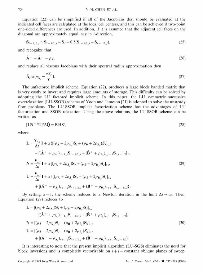
It is interesting to note that the present implicit algorithm (LU-SGS) eliminates the need forblock inversions and is completely vectorizable on i+ j=constant oblique planes of sweep.



3.3. Boundary conditions

The boundary conditions imposed on the solid surface are the no-slip condition for viscousflows and the tangency condition for inviscid flows. A zero normal pressure gradient on thewall is applied. In the far-field, a locally one-dimensional characteristic-type of boundarycondition is used. The procedures employed here are similar to those usually used for thecompressible flows. The Riemann invariants for this system of equations are now given by

R9=p+12

un29

12

[unc+b ln(un+c)], (31)

where un is the component of the velocity normal to the boundary. In all calculations, theabove boundary conditions are treated explicitly.

4. RESULTS AND DISCUSSION

Presented in this section are the results of four different laminar flow computations. For thesteady cases, these are driven cavity flow and flow over a backward-facing step. For theunsteady cases, these are flow decayed by viscosity and flow over a circular cylinder.

4.1. Dri6en ca6ity flow

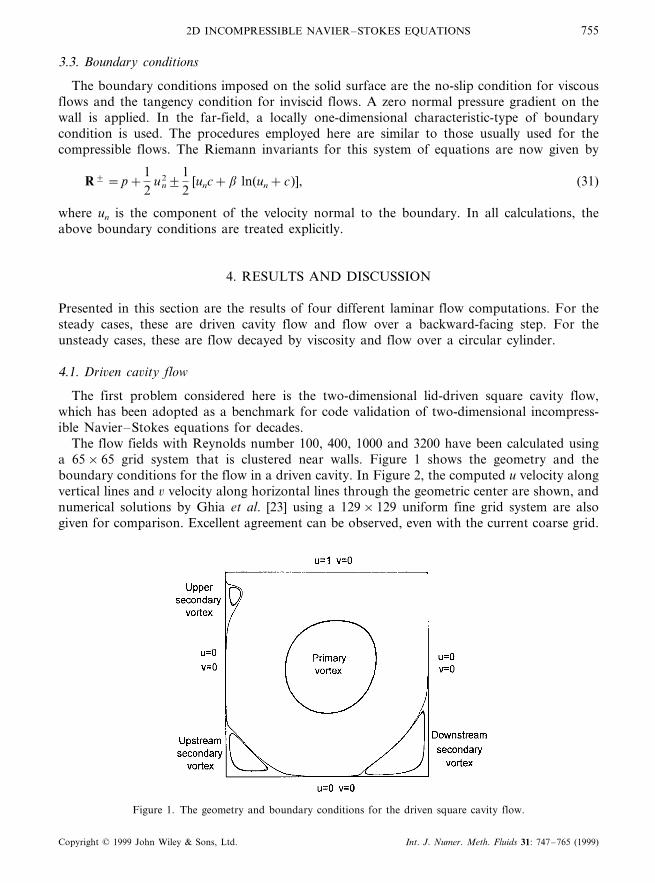
The first problem considered here is the two-dimensional lid-driven square cavity flow,which has been adopted as a benchmark for code validation of two-dimensional incompress-ible Navier–Stokes equations for decades.

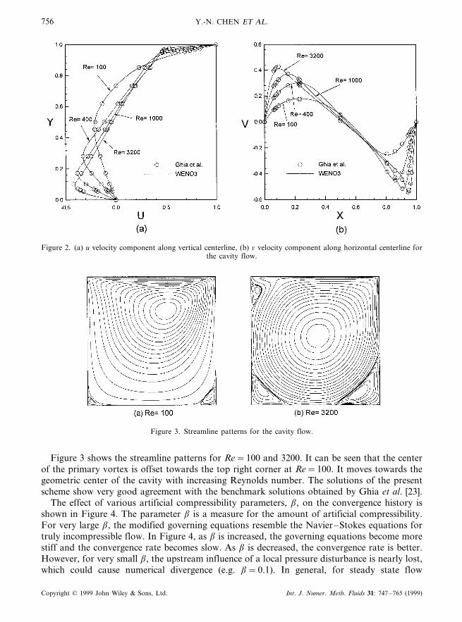
The flow fields with Reynolds number 100, 400, 1000 and 3200 have been calculated usinga 65×65 grid system that is clustered near walls. Figure 1 shows the geometry and theboundary conditions for the flow in a driven cavity. In Figure 2, the computed u velocity alongvertical lines and 6 velocity along horizontal lines through the geometric center are shown, andnumerical solutions by Ghia et al. [23] using a 129×129 uniform fine grid system are alsogiven for comparison. Excellent agreement can be observed, even with the current coarse grid.

Figure 1. The geometry and boundary conditions for the driven square cavity flow.



Figure 2. (a) u velocity component along vertical centerline, (b) 6 velocity component along horizontal centerline forthe cavity flow.

Figure 3. Streamline patterns for the cavity flow.

Figure 3 shows the streamline patterns for Re=100 and 3200. It can be seen that the centerof the primary vortex is offset towards the top right corner at Re=100. It moves towards thegeometric center of the cavity with increasing Reynolds number. The solutions of the presentscheme show very good agreement with the benchmark solutions obtained by Ghia et al. [23].

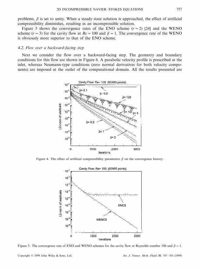
The effect of various artificial compressibility parameters, b, on the convergence history isshown in Figure 4. The parameter b is a measure for the amount of artificial compressibility.For very large b, the modified governing equations resemble the Navier–Stokes equations fortruly incompressible flow. In Figure 4, as b is increased, the governing equations become morestiff and the convergence rate becomes slow. As b is decreased, the convergence rate is better.However, for very small b, the upstream influence of a local pressure disturbance is nearly lost,which could cause numerical divergence (e.g. b=0.1). In general, for steady state flow



problems, b is set to unity. When a steady state solution is approached, the effect of artificialcompressibility diminishes, resulting in an incompressible solution.

Figure 5 shows the convergence rates of the ENO scheme (r=2) [24] and the WENOscheme (r=3) for the cavity flow at Re=100 and b=1. The convergence rate of the WENOis obviously more superior to that of the ENO scheme.

4.2. Flow o6er a backward-facing step

Next we consider the flow over a backward-facing step. The geometry and boundaryconditions for this flow are shown in Figure 6. A parabolic velocity profile is prescribed at theinlet, whereas Neumann-type conditions (zero normal derivatives for both velocity compo-nents) are imposed at the outlet of the computational domain. All the results presented are

Figure 4. The effect of artificial compressibility parameters b on the convergence history.

Figure 5. The convergence rate of ENO and WENO schemes for the cavity flow at Reynolds number 100 and b=1.



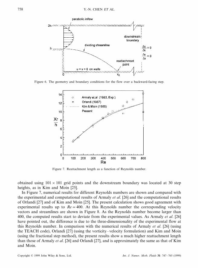
Figure 6. The geometry and boundary conditions for the flow over a backward-facing step.

Figure 7. Reattachment length as a function of Reynolds number.

obtained using 101×101 grid points and the downstream boundary was located at 30 stepheights, as in Kim and Moin [25].

In Figure 7, numerical results for different Reynolds numbers are shown and compared withthe experimental and computational results of Armaly et al. [26] and the computational resultsof Orlandi [27] and of Kim and Moin [25]. The present calculation shows good agreement withexperimental results up to Re=400. At this Reynolds number the corresponding velocityvectors and streamlines are shown in Figure 8. As the Reynolds number become larger than400, the computed results start to deviate from the experimental values. As Armaly et al. [26]have pointed out, the difference is due to the three-dimensionality of the experimental flow atthis Reynolds number. In comparison with the numerical results of Armaly et al. [26] (usingthe TEACH code), Orlandi [27] (using the vorticity–velocity formulation) and Kim and Moin(using the fractional step method), the present results show a much higher reattachment lengththan those of Armaly et al. [26] and Orlandi [27], and is approximately the same as that of Kimand Moin.



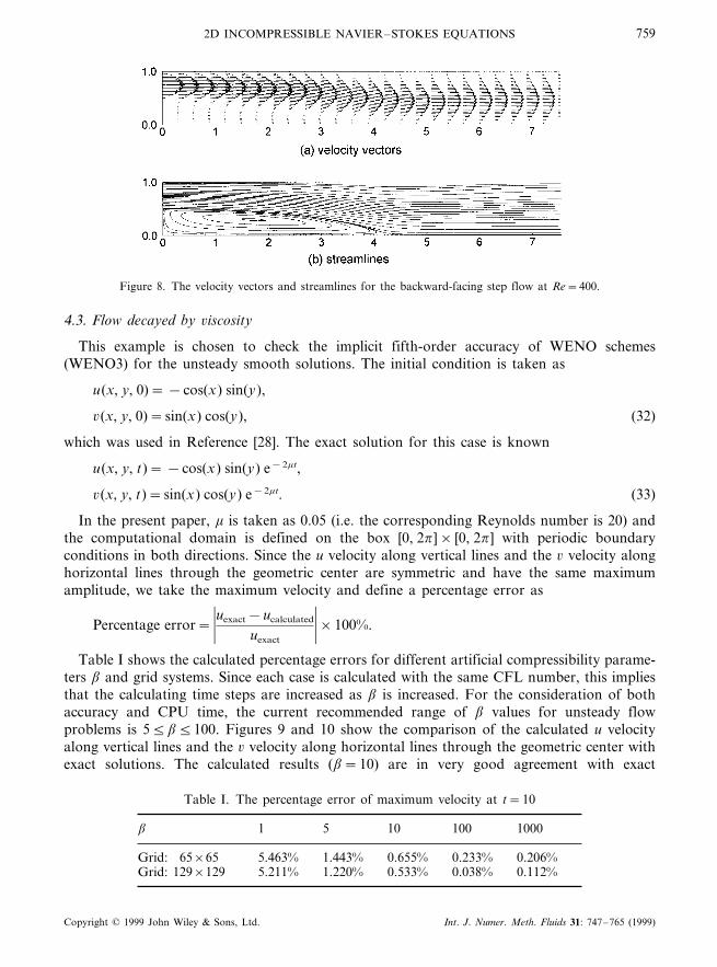
Figure 8. The velocity vectors and streamlines for the backward-facing step flow at Re=400.

4.3. Flow decayed by 6iscosity

This example is chosen to check the implicit fifth-order accuracy of WENO schemes(WENO3) for the unsteady smooth solutions. The initial condition is taken as

u(x, y, 0)= −cos(x) sin(y),

6(x, y, 0)=sin(x) cos(y), (32)

which was used in Reference [28]. The exact solution for this case is known

u(x, y, t)= −cos(x) sin(y) e−2mt,

6(x, y, t)=sin(x) cos(y) e−2mt. (33)

In the present paper, m is taken as 0.05 (i.e. the corresponding Reynolds number is 20) andthe computational domain is defined on the box [0, 2p ]× [0, 2p ] with periodic boundaryconditions in both directions. Since the u velocity along vertical lines and the 6 velocity alonghorizontal lines through the geometric center are symmetric and have the same maximumamplitude, we take the maximum velocity and define a percentage error as

Percentage error=)uexact−ucalculated

uexact

)×100%.

Table I shows the calculated percentage errors for different artificial compressibility parame-ters b and grid systems. Since each case is calculated with the same CFL number, this impliesthat the calculating time steps are increased as b is increased. For the consideration of bothaccuracy and CPU time, the current recommended range of b values for unsteady flowproblems is 55b5100. Figures 9 and 10 show the comparison of the calculated u velocityalong vertical lines and the 6 velocity along horizontal lines through the geometric center withexact solutions. The calculated results (b=10) are in very good agreement with exact

Table I. The percentage error of maximum velocity at t=10

1 5b 10 100 1000

0.655% 0.233% 0.206%Grid: 65×65 5.463% 1.443%0.533% 0.038% 0.112%Grid: 129×129 5.211% 1.220%



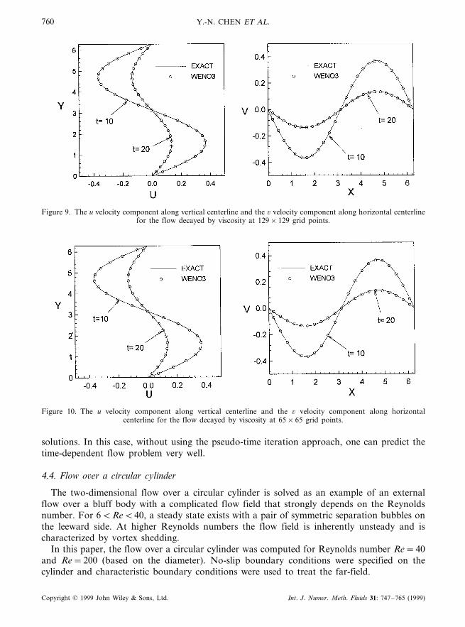
Figure 9. The u velocity component along vertical centerline and the 6 velocity component along horizontal centerlinefor the flow decayed by viscosity at 129×129 grid points.

Figure 10. The u velocity component along vertical centerline and the 6 velocity component along horizontalcenterline for the flow decayed by viscosity at 65×65 grid points.

solutions. In this case, without using the pseudo-time iteration approach, one can predict thetime-dependent flow problem very well.

4.4. Flow o6er a circular cylinder

The two-dimensional flow over a circular cylinder is solved as an example of an externalflow over a bluff body with a complicated flow field that strongly depends on the Reynoldsnumber. For 6BReB40, a steady state exists with a pair of symmetric separation bubbles onthe leeward side. At higher Reynolds numbers the flow field is inherently unsteady and ischaracterized by vortex shedding.

In this paper, the flow over a circular cylinder was computed for Reynolds number Re=40and Re=200 (based on the diameter). No-slip boundary conditions were specified on thecylinder and characteristic boundary conditions were used to treat the far-field.



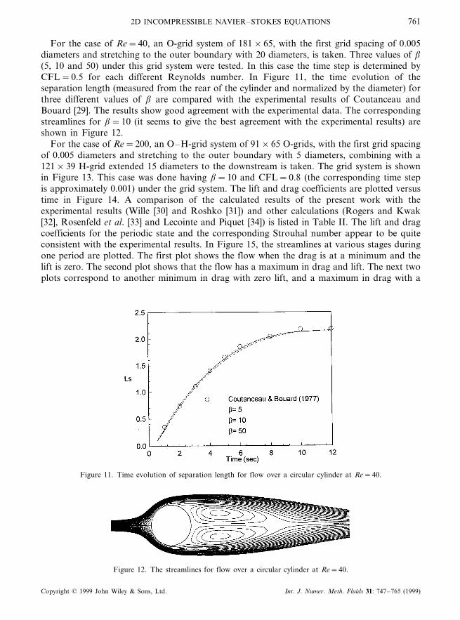
For the case of Re=40, an O-grid system of 181×65, with the first grid spacing of 0.005diameters and stretching to the outer boundary with 20 diameters, is taken. Three values of b

(5, 10 and 50) under this grid system were tested. In this case the time step is determined byCFL=0.5 for each different Reynolds number. In Figure 11, the time evolution of theseparation length (measured from the rear of the cylinder and normalized by the diameter) forthree different values of b are compared with the experimental results of Coutanceau andBouard [29]. The results show good agreement with the experimental data. The correspondingstreamlines for b=10 (it seems to give the best agreement with the experimental results) areshown in Figure 12.

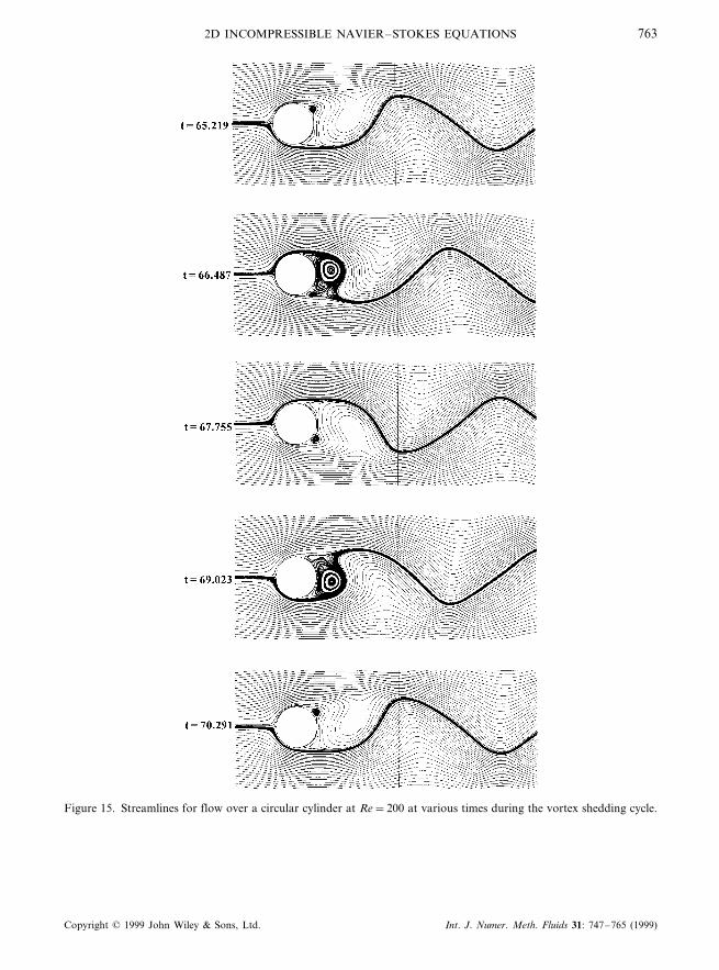
For the case of Re=200, an O–H-grid system of 91×65 O-grids, with the first grid spacingof 0.005 diameters and stretching to the outer boundary with 5 diameters, combining with a121×39 H-grid extended 15 diameters to the downstream is taken. The grid system is shownin Figure 13. This case was done having b=10 and CFL=0.8 (the corresponding time stepis approximately 0.001) under the grid system. The lift and drag coefficients are plotted versustime in Figure 14. A comparison of the calculated results of the present work with theexperimental results (Wille [30] and Roshko [31]) and other calculations (Rogers and Kwak[32], Rosenfeld et al. [33] and Lecointe and Piquet [34]) is listed in Table II. The lift and dragcoefficients for the periodic state and the corresponding Strouhal number appear to be quiteconsistent with the experimental results. In Figure 15, the streamlines at various stages duringone period are plotted. The first plot shows the flow when the drag is at a minimum and thelift is zero. The second plot shows that the flow has a maximum in drag and lift. The next twoplots correspond to another minimum in drag with zero lift, and a maximum in drag with a

Figure 11. Time evolution of separation length for flow over a circular cylinder at Re=40.

Figure 12. The streamlines for flow over a circular cylinder at Re=40.



Figure 13. The computational grid system for flow over a circular cylinder at Re=200.

Figure 14. Lift and drag coefficients vs. time for flow over a circular cylinder at Re=200.

Table II. Lift and drag coefficients and Strouhal numbers for circular cylinderflow at Re=200

CL StCD

90.72 0.197Present 1.3390.04

0.16090.751.2990.05third-orderRogers and Kwak [32]0.185fifth-order 1.2390.05 90.650.201Rosenfeld et al. [33] 1.4090.04 90.70

1.4690.04 0.22790.70second-orderLecointe and Piquet [34]0.194fourth-order 1.5890.0035 90.50

Wille (experimental) [30] 1.30.19Roshko (experimental) [31]

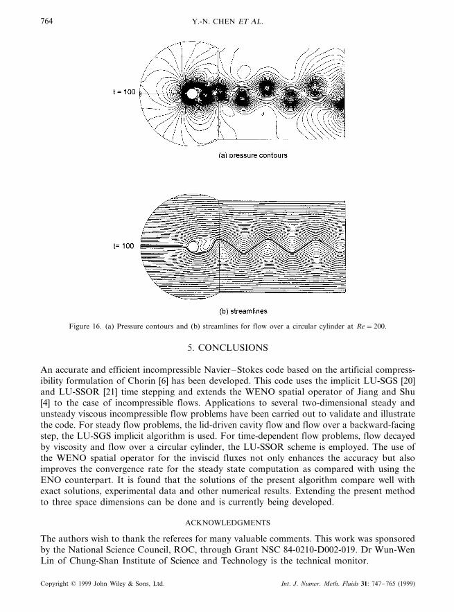
minimum in lift respectively. These two are mirror images of the first two plots. Finally, thelast plot is identical to the first one, and the period for this flow is 5.072 (i.e. the correspondingStrouhal number is 0.197). To show the vortex shedding phenomenon, the pressure contoursand streamlines covering the whole computational domain are shown in Figure 16.



Figure 15. Streamlines for flow over a circular cylinder at Re=200 at various times during the vortex shedding cycle.



Figure 16. (a) Pressure contours and (b) streamlines for flow over a circular cylinder at Re=200.

5. CONCLUSIONS

An accurate and efficient incompressible Navier–Stokes code based on the artificial compress-ibility formulation of Chorin [6] has been developed. This code uses the implicit LU-SGS [20]and LU-SSOR [21] time stepping and extends the WENO spatial operator of Jiang and Shu[4] to the case of incompressible flows. Applications to several two-dimensional steady andunsteady viscous incompressible flow problems have been carried out to validate and illustratethe code. For steady flow problems, the lid-driven cavity flow and flow over a backward-facingstep, the LU-SGS implicit algorithm is used. For time-dependent flow problems, flow decayedby viscosity and flow over a circular cylinder, the LU-SSOR scheme is employed. The use ofthe WENO spatial operator for the inviscid fluxes not only enhances the accuracy but alsoimproves the convergence rate for the steady state computation as compared with using theENO counterpart. It is found that the solutions of the present algorithm compare well withexact solutions, experimental data and other numerical results. Extending the present methodto three space dimensions can be done and is currently being developed.

ACKNOWLEDGMENTS

The authors wish to thank the referees for many valuable comments. This work was sponsoredby the National Science Council, ROC, through Grant NSC 84-0210-D002-019. Dr Wun-WenLin of Chung-Shan Institute of Science and Technology is the technical monitor.



REFERENCES

1. A. Harten, B. Engquist, S. Osher and S. Chakravarthy, ‘Uniformly high-order accurate nonoscillatory schemes’,J. Comput. Phys., 71, 231–303 (1987).

2. C.-W. Shu and S. Osher, ‘Efficient implementation of nonoscillatory shock capturing schemes’, J. Comput. Phys.,77, 439–471 (1988).

3. C.-W. Shu and S. Osher, ‘Efficient implementation of nonoscillatory shock capturing schemes, II’, J. Comput.Phys., 83, 32–78 (1988).

4. G.S. Jiang and C.-W. Shu, ‘Efficient implementation of weighted ENO schemes’, J. Comput. Phys., 126, 202–228(1996).

5. X.-D. Liu, S. Osher and T. Chan, ‘Weighted essentially nonoscillatory schemes’, J. Comput. Phys., 115, 200–212(1994).

6. A.J. Chorin, ‘A numerical method for solving incompressible viscous flow problems’, J. Comput. Phys., 2, 12–26(1967).

7. R.M. Beam and R.F. Warming, ‘An implicit factored scheme for the compressible Navier–Stokes equations’,AIAA J., 16, 393–402 (1978).

8. J.L. Steger and P. Kutler, ‘Implicit finite difference procedures for the computation of vortex wakes’, AIAA J., 15,581–590 (1977).

9. D. Choi and C.L. Merkle, ‘Application of time-iterative schemes to incompressible flow’, AIAA J., 23, 1518–1524(1985).

10. D. Kwak, J.L.C. Chang, S.P. Shanks and S.R. Chakravarthy, ‘A three-dimensional incompressible Navier–Stokesflow solver using primitive variables’, AIAA J., 24, 390–396 (1986).

11. J.L.C. Chang, D. Kwak and S.C. Dao, ‘A three-dimensional incompressible flow simulation method and itsapplication to the space shuttle main engine. Part I. Laminar flow’, AIAA Paper 85-0175, 1985.

12. J.L.C. Chang, D. Kwak, S.C. Dao and R. Rosen, ‘A three-dimensional incompressible flow simulation methodand its application to the space shuttle main engine. Part II. Turbulent flow’, AIAA Paper 85-1670, 1985.

13. J.L.C. Chang and D. Kwak, ‘Numerical study of turbulent internal shear layer flow in an axisymmetric U-duct’,AIAA Paper 88-0596, 1988.

14. J.L.C. Chang, D. Kwak, S.E. Rogers and R.J. Yang, ‘Numerical simulation methods of incompressible flows andan application to the space shuttle main engine’, Int. J. Numer. Methods Fluids, 8, 1241–1268 (1988).

15. C.L. Merkle and M. Athavale, ‘Time-accurate unsteady incompressible flow algorithms based on artificialcompressibility’, AIAA Paper 87-1137, 1987.

16. S.E. Rogers and D. Kwak, ‘An upwind differencing scheme for the time-accurate incompressible Navier–Stokesequations’, AIAA Paper 88-2583, 1988.

17. S.E. Rogers, D. Kwak and C. Kiris, ‘Numerical solution of the incompressible Navier–Stokes equations forsteady state and time-dependent problems’, AIAA Paper 89-0463, 1989.

18. W.K. Anderson, R.D. Rausch and D.L. Bonhaus, ‘Implicit/multigrid algorithms for incompressible turbulentflows on unstructured grids’, AIAA-95-1740-CP, 1995.

19. W.R. Briley, S.S. Neerarambam and D.L. Whitfield, ‘Implicit lower–upper/approximate-factorization algorithmsfor viscous incompressible flows’, AIAA-95-l742-CP, 1995.

20. S. Yoon, D. Kwak and L. Chang, ‘LU-SGS implicit algorithm for three-dimensional incompressible Navier–Stokes equations with source term’, AIAA Paper 89-196l-CP, 1989.

21. S. Yoon and A. Jameson, ‘An LU-SSOR scheme for the Euler and Navier–Stokes equaions’, AIAA Paper87-0600, 1987.

22. A. Jameson and S. Yoon, ‘Lower–upper implicit schemes with multiple grids for the Euler equations’, AIAA J.,25, 929–935 (1987).

23. U. Ghia, K.N. Ghia and C.T. Shin, ‘High-Re solutions for incompressible flow using the Navier–Stokes equationsand a multigrid method’, J. Comput. Phys., 48, 387–411 (1982).

24. J.Y. Yang and C.A. Hsu, ‘High-resolution, nonoscillatory schemes for unsteady compressible flows’, AIAA J., 30,1570–1575 (1992).

25. J. Kim and P. Moin, ‘Application of a fractional-step method to incompressible Navier–Stokes equations’, J.Comput. Phys., 59, 308–323 (1985).

26. B.F. Armaly, F. Durst, J.C.F. Pereira and B. Schonung, ‘Experimental and theoretical investigation of backward-facing step flow’, J. Fluid Mech., 127, 473–496 (1983).

27. P. Orlandi, ‘Vorticity–velocity formulation for high Re flows’, Comput. Fluids, 15, 137–149 (1987).28. A.J. Chorin, ‘Numerical solution of Navier–Stokes equations’, Math. Comput., 22, 740–762 (1968).29. M. Coutanceau and R. Bouard, ‘Experimental determination of the main features of the viscous flow in the wake

of a circular cylinder in uniform translation. Part 2. Unsteady flow’, J. Fluid Mech., 79, 257–272 (1977).30. R. Wille, ‘Karman vortex streets’, Ad6. Appl. Mech., 6, 273 (1960).31. A. Roshko, ‘On the development of turbulent wakes from vortex streets’, NACA Report 1191, 1954.32. S.E. Rogers and D. Kwak, ‘An upwind differencing scheme for the time-accurate incompressible Navier–Stokes

equations’, AIAA Paper 88-2583, 1988.33. M. Rosenfeld, D. Kwak and M. Vinokur, ‘A solution method for the unsteady and incompressible Navier–Stokes

equations in generalized coordinate systems’, AIAA Paper 88-0718, 1988.34. Y. Lecointe and J. Piquet, ‘On the use of several compact methods for the study of unsteady incompressible

viscous flow round a circular cylinder’, Comput. Fluids, 12, 255–280 (1984).


Documents

Implicit weighted essentially non-oscillatory schemes … · IMPLICIT WEIGHTED ESSENTIALLY NON-OSCILLATORY SCHEMES FOR THE ... for compressible flows, ... In order to apply compressible