Embed Size (px)
Citation preview
High order finite difference WENO schemes for nonlinear degenerate
parabolic equations
Yuanyuan Liu1, Chi-Wang Shu2 and Mengping Zhang3
Abstract
High order accurate weighted essentially non-oscillatory (WENO) schemes are usu-
ally designed to solve hyperbolic conservation laws or to discretize the first derivative
convection terms in convection dominated partial differential equations. In this paper
we discuss a high order WENO finite difference discretization for nonlinear degenerate
parabolic equations which may contain discontinuous solutions. A porous medium equa-
tion is used as an example to demonstrate the algorithm structure and performance. Two
different formulations of WENO schemes, one approximating directly the second deriva-
tive term using a conservative flux difference, and another approximating this term by
first rewriting it as two first derivative terms using an auxiliary variable before applying
the WENO procedure on those first derivatives, are discussed and compared. Numerical
examples are provided to demonstrate the accuracy and non-oscillatory performance of
these schemes.
Key Words: Weighted essentially non-oscillatory (WENO) scheme, finite difference
scheme, nonlinear degenerate parabolic equation, porous medium equation
1Department of Mathematics, University of Science and Technology of China, Hefei, Anhui 230026,P.R. China. E-mail: [email protected]
2Division of Applied Mathematics, Brown University, Providence, RI 02912, USA. E-mail:[email protected]. Research supported by ARO grant W911NF-08-1-0520 and NSF grant DMS-0809086.
3Department of Mathematics, University of Science and Technology of China, Hefei, Anhui 230026,P.R. China. E-mail: [email protected]. Research supported by NSFC grant 10671190.
1

1 Introduction
Weighted essentially non-oscillatory (WENO) schemes were introduced in the literature
to approximate hyperbolic conservation laws and the first derivative convection terms
in convection dominated convection diffusion partial differential equations (PDEs). The
first WENO scheme was introduced in 1994 by Liu, Osher and Chan in their pioneering
paper [19], in which a third order accurate finite volume WENO scheme in one space
dimension was constructed. In 1996, Jiang and Shu [15] provided a general framework to
design arbitrary order accurate finite difference WENO schemes, which are more efficient
for multi-dimensional calculations. Very high order WENO schemes are documented in
[3]. All these papers use the WENO reconstruction procedure, which is equivalent to
a conservative WENO approximation for the first derivative, and is the main relevant
WENO procedure for designing both conservative finite volume and conservative finite
difference schemes to solve hyperbolic conservation laws.
It was realized later that the WENO procedure can also be used in different contexts,
for example in WENO interpolation and in WENO integration. The WENO interpo-
lation procedure is used, for example, in [26] to transfer information from one domain
to another in a high order, non-oscillatory fashion for a multi-domain WENO scheme,
and in [6] to build a high order Lagrangian type method for solving Hamilton-Jacobi
equations. The WENO integration procedure is used, for example, in [8, 9] for the de-
sign of high order residual distribution conservative finite difference WENO schemes. In
our recent work [20] we have studied the positivity of linear weights for various WENO
procedures, including reconstruction, interpolation, integration, and approximations to
higher order derivatives. For an extensive review on WENO schemes, see [29].
In this paper, we are interested in designing WENO schemes for solving the following
nonlinear, possibly degenerate parabolic equations
ut = b(u)xx (1.1)
2

where a(u) = b′(u) ≥ 0 and it is possible that a(u) = 0 for certain values of u. Such equa-
tions appear often in applications. For example, the following porous medium equation
(PME) modelled in [22, 2]
ut = (um)xx (1.2)
in which m is a constant greater than one, belongs to this class. This equation describes
various diffusion processes, for example the flow of an isentropic gas through a porous
medium, where u is the density of the gas required to be nonnegative and um−1 is the
pressure of the gas. Clearly, the equation degenerates at points where u = 0, resulting
in the phenomenon of finite speed of propagation and discontinuous solutions.
The famous Barenblatt solution of the PME (1.2) is found in 1950 by Zel’dovich and
Kompaneetz [31] (see also Barenblatt [4]), which is defined explicitly by
Bm(x, t) = t−k
[(
1 −k(m − 1)
2m
|x|2
t2k
)
+
]1/(m−1)
, m > 1. (1.3)
where u+ = max(u, 0) and k = (m + 1)−1. This solution, for any time t > 0, has a
compact support [−αm(t), αm(t)] with the interface |x| = αm(t) moving outward in a
finite speed, where
αm(t) =
√
2m
k(m − 1)tk.
The Barenblatt solution shows that solutions to the PME may have the following prop-
erties:
1. Finite speed of propagation: If the initial function has compact support, then at
all times the solution u(·, t) will have compact support.
2. Free-boundaries: The interface behaves like a free-boundary propagating with finite
speed.
3. Weak solutions: Since there exists no derivative at the interface points |x| = αm(t).
Various schemes for approximating (1.1) have been developed in the literature. Lin-
ear approximation schemes based on the nonlinear Chernoff’s formula with a suitable
3
relaxation parameter have been studied in, e.g. [5, 23, 24, 21], where energy error
estimates have also been investigated. See also [14, 16] for other types of linear ap-
proximation schemes. More recently, a different approach based on kinetic schemes for
degenerate parabolic systems has been considered in [1]. Other approaches include that
in [11], which is based on a suitable splitting technique with applications to more general
hyperbolic-parabolic convection-diffusion equations, and that in [25], which is based on
the maximum principle and on perturbation and regularization. A high order relaxation
scheme has been presented in [7]. Finally a local discontinuous Galerkin finite element
method has been constructed in [32] for the porous medium equation.
The degenerate parabolic equation (1.1) has similar features as a hyperbolic con-
servation law, such as the possible existence of discontinuous solutions and finite speed
of propagation of wave fronts. Therefore, it is reasonable to generalize numerical tech-
niques for solving hyperbolic conservation laws, such as the WENO technique, to solve
the equation (1.1). This would involve a careful adaptation of the WENO procedure, to
ensure conservation, accuracy and non-oscillatory performance. In this paper we discuss
two different formulations of WENO schemes for approximating (1.1). The first formu-
lation, discussed in Section 2, approximates directly the second derivative term using a
conservative flux difference. This approach involves a narrower stencil for a given order
of accuracy, however it would necessarily involve the usage of negative linear weights,
therefore requiring a special treatment as in [27] to ensure non-oscillatory performance of
the resulting WENO scheme. The second approach, discussed in Section 3, starts with
the introduction of an auxiliary variable for the first derivative, then applies the WENO
procedure to two first derivatives rather than to the second derivative term directly. This
resembles the approach of the local discontinuous Galerkin method [10]. This approach
requires only WENO approximations to first derivatives, which is a relatively mature
procedure and avoids the appearance of negative linear weights. However, the compu-
tational cost is larger since two WENO approximations rather than one must be used
4

to approximate the second derivative. The effective stencil, which is a composition of
two successive WENO procedures, is also wider in comparison with the first approach.
We provide numerical examples to demonstrate the accuracy and non-oscillatory perfor-
mance of these two types of WENO schemes and give a comparison.
2 Direct WENO discretization to the second deriva-
tive
In this section we study a direct WENO discretization to the second derivative in conser-
vation form. Assume that we have a mesh · · · < x1 < x2 < x3 < · · · , and for simplicity
we assume the grid is uniform, i.e. ∆x = xi+1 − xi is constant. We are building a
conservative finite difference scheme for the equation (1.1), written in the form
dui(t)
dt=
fi+ 12− fi− 1
2
∆x2. (2.1)
where ui(t) is the numerical approximation to the point value u(xi, t) of the solution to
(1.1), and the numerical flux function
fi+ 12
= f(ui−r, . . . , ui+s), (2.2)
is chosen so that the conservative difference on the right hand side of the scheme (2.1)
approximates the second order derivative (b(u))xx at x = xi to high order accuracy
fi+ 12− fi− 1
2
∆x2= (b(u))xx|x=xi
+ O(∆xk) (2.3)
when the solution is smooth, and would generate non-oscillatory solutions when the
solution contains possible discontinuities. The collection of grid points involved in the
numerical flux (2.2), S = {xi−r, . . . , xi+s}, is called the stencil of the flux approximation.
A linear scheme is a scheme for which the numerical flux (2.2) is a linear combination of
the grid values in the stencil
fi+ 12
=
s∑
j=−r
ajb(ui+j). (2.4)
5

where the constant coefficients aj can be chosen to yield the highest order of accuracy k
in (2.3). For example, the classical second order scheme
dui(t)
dt=
b(ui+1) − 2b(ui) + b(ui−1)
∆x2(2.5)
corresponds to the numerical flux with the stencil S = {xi, xi+1} and is given by
fi+ 12
= −b(ui) + b(ui+1).
The construction of WENO schemes in this section consists of the following steps.
1. We choose a symmetric big stencil, S = {xi−r, . . . , xi+r+1}, for the numerical flux
(2.4), resulting in a linear scheme with an order of accuracy k = 2r + 2 in (2.3).
This linear scheme should be stable with the designed high order accuracy for
smooth solutions, but will be oscillatory near discontinuities.
2. We choose s consecutive small stencils, Sm = {xi−r+m, . . . , xi+r+m+2−s}, for m =
0, . . . , s − 1, resulting in a series of lower order linear schemes with their numer-
ical fluxes denoted by f(m)
i+ 12
. Here, s can be chosen to be between 2 and 2r + 1,
corresponding to each small stencil containing 2r + 1 to 2 points, respectively.
3. We find the linear weights, namely constants dm, such that the flux on the big
stencil is a linear combination of the fluxes on the small stencils with dm as the
combination coefficients
fi+ 12
=
s−1∑
m=0
dm f(m)
i+ 12
. (2.6)
If we simply use the linear weights and linear combination on the right hand side
of (2.6), we would get back the linear scheme on the big stencil, which will be
accurate for smooth solutions but will be oscillatory near discontinuities.
4. We change the linear weights dm in (2.6) to nonlinear weights ωm, with the ob-
jective of maintaining the same high order accuracy for smooth solutions and
non-oscillatory performance near discontinuities. This is usually achieved through
6
smoothness indicators which measure the smoothness of the function based on
different small stencils.
If the linear weights dm obtained in the third step above are non-negative, then the
linear combination in (2.6) is a convex combination, since by consistency∑s−1
m=0 dm = 1.
This will help significantly in the design of nonlinear weights in the fourth step above. In
[20], we studied the positivity of linear weights for various WENO procedures. However,
the current conservative approximation to the second derivative is not considered in [20].
We will therefore start with a discussion on the positivity of the linear weights below,
with a rather disappointing conclusion that negative linear weights must appear.
2.1 Analysis of the linear weights
In this subsection we study the linear weights dm in (2.6). In particular, we conclude
that it is not possible to maintain all of them non-negative. We consider the cases of
r = 1, 2 and 3, namely the big stencil containing 4, 6 and 8 points, corresponding to
central schemes of fourth, sixth and eighth order accuracy, respectively.
The linear weights in (2.6), for various numbers of small stencils, are listed in Table
2.1. We conclude from this table that in some cases the linear weights do not exist for
(2.6) to hold, and when they do exist, at least one of them is negative.
We give below the details for the situation r = 2, corresponding to 6 points in the
big stencil, including the coefficients aj in (2.4).
The big stencil in this case is given by
S = {xi−2, xi−1, xi, xi+1, xi+2, xi+3},
and the flux (2.4) corresponding to the big stencil is given by
fi+ 12
=−2b(ui−2) + 25b(ui−1) − 245b(ui) + 245b(ui+1) − 25b(ui+2) + 2b(ui+3)
180,
corresponding to a sixth order central scheme. Depending on the number of small sten-
cils, we have the following situations.
7
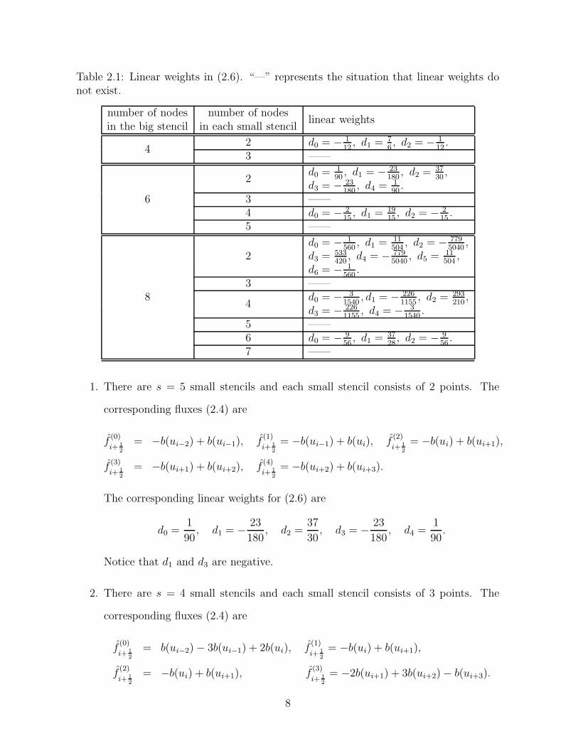
Table 2.1: Linear weights in (2.6). “—” represents the situation that linear weights donot exist.
number of nodes number of nodeslinear weights
in the big stencil in each small stencil
42 d0 = − 1
12, d1 = 7
6, d2 = − 1
12.
3 ——
6
2d0 = 1
90, d1 = − 23
180, d2 = 37
30,
d3 = − 23180
, d4 = 190
.3 ——4 d0 = − 2
15, d1 = 19
15, d2 = − 2
15.
5 ——
8
2d0 = − 1
560, d1 = 11
504, d2 = − 779
5040,
d3 = 533420
, d4 = − 7795040
, d5 = 11504
,d6 = − 1
560.
3 ——
4d0 = − 3
1540, d1 = − 226
1155, d2 = 293
210,
d3 = − 2261155
, d4 = − 31540
.5 ——6 d0 = − 9
56, d1 = 37
28, d2 = − 9
56.
7 ——
1. There are s = 5 small stencils and each small stencil consists of 2 points. The
corresponding fluxes (2.4) are
f(0)
i+ 12
= −b(ui−2) + b(ui−1), f(1)
i+ 12
= −b(ui−1) + b(ui), f(2)
i+ 12
= −b(ui) + b(ui+1),
f(3)
i+ 12
= −b(ui+1) + b(ui+2), f(4)
i+ 12
= −b(ui+2) + b(ui+3).
The corresponding linear weights for (2.6) are
d0 =1
90, d1 = −
23
180, d2 =
37
30, d3 = −
23
180, d4 =
1
90.
Notice that d1 and d3 are negative.
2. There are s = 4 small stencils and each small stencil consists of 3 points. The
corresponding fluxes (2.4) are
f(0)
i+ 12
= b(ui−2) − 3b(ui−1) + 2b(ui), f(1)
i+ 12
= −b(ui) + b(ui+1),
f(2)
i+ 12
= −b(ui) + b(ui+1), f(3)
i+ 12
= −2b(ui+1) + 3b(ui+2) − b(ui+3).
8
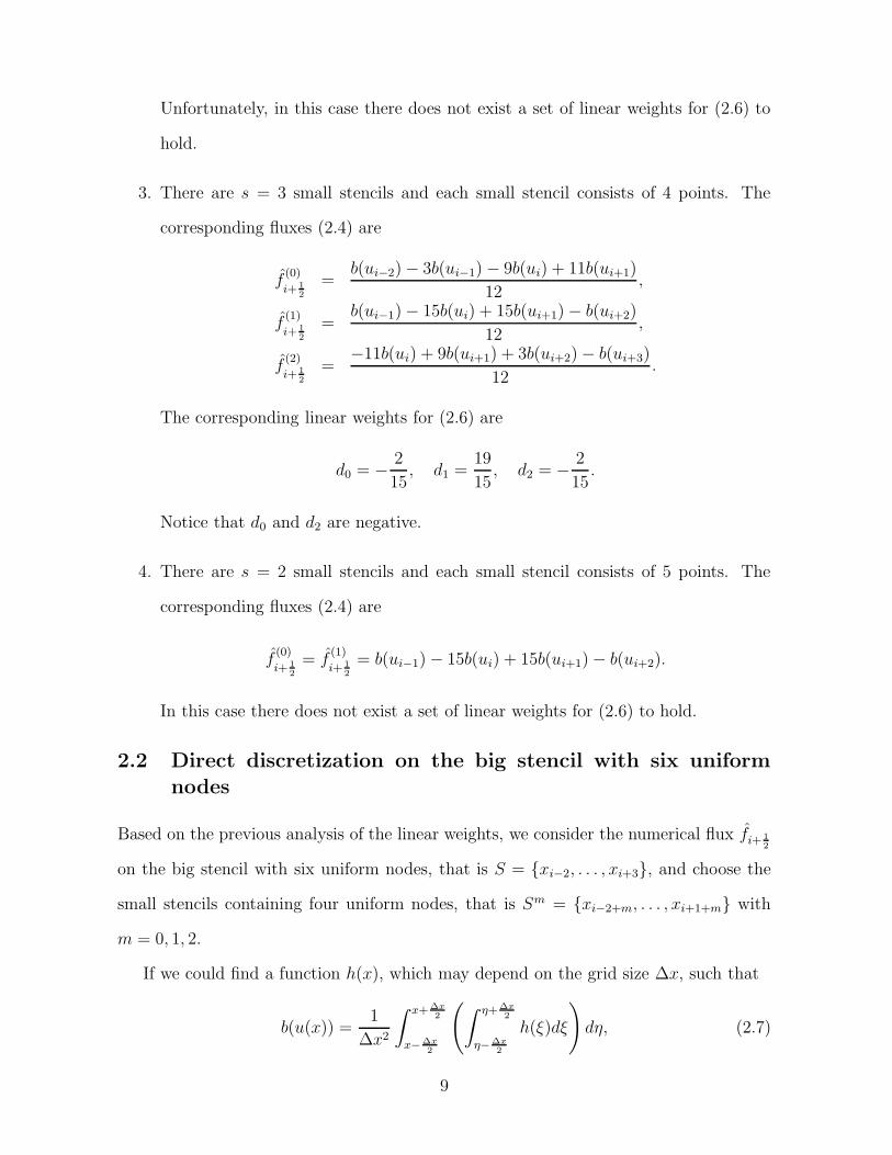
Unfortunately, in this case there does not exist a set of linear weights for (2.6) to
hold.
3. There are s = 3 small stencils and each small stencil consists of 4 points. The
corresponding fluxes (2.4) are
f(0)
i+ 12
=b(ui−2) − 3b(ui−1) − 9b(ui) + 11b(ui+1)
12,
f(1)
i+ 12
=b(ui−1) − 15b(ui) + 15b(ui+1) − b(ui+2)
12,
f(2)
i+ 12
=−11b(ui) + 9b(ui+1) + 3b(ui+2) − b(ui+3)
12.
The corresponding linear weights for (2.6) are
d0 = −2
15, d1 =
19
15, d2 = −
2
15.
Notice that d0 and d2 are negative.
4. There are s = 2 small stencils and each small stencil consists of 5 points. The
corresponding fluxes (2.4) are
f(0)
i+ 12
= f(1)
i+ 12
= b(ui−1) − 15b(ui) + 15b(ui+1) − b(ui+2).
In this case there does not exist a set of linear weights for (2.6) to hold.
2.2 Direct discretization on the big stencil with six uniform
nodes
Based on the previous analysis of the linear weights, we consider the numerical flux fi+ 12
on the big stencil with six uniform nodes, that is S = {xi−2, . . . , xi+3}, and choose the
small stencils containing four uniform nodes, that is Sm = {xi−2+m, . . . , xi+1+m} with
m = 0, 1, 2.
If we could find a function h(x), which may depend on the grid size ∆x, such that
b(u(x)) =1
∆x2
∫ x+∆x2
x−∆x2
(
∫ η+∆x2
η−∆x2
h(ξ)dξ
)
dη, (2.7)
9
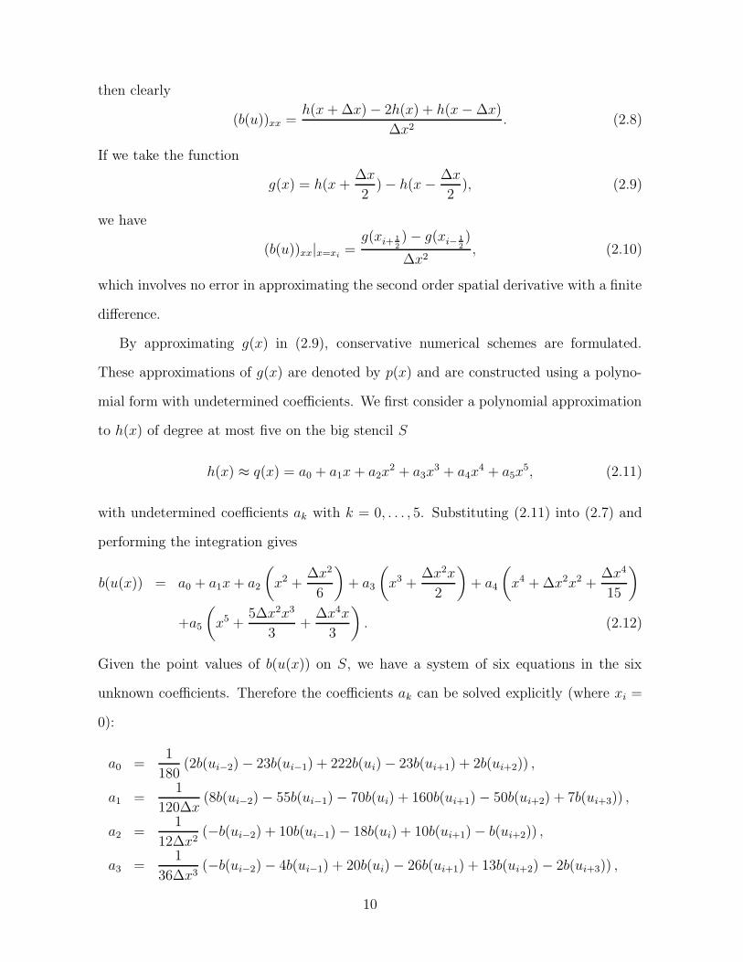
then clearly
(b(u))xx =h(x + ∆x) − 2h(x) + h(x − ∆x)
∆x2. (2.8)
If we take the function
g(x) = h(x +∆x
2) − h(x −
∆x
2), (2.9)
we have
(b(u))xx|x=xi=
g(xi+ 12) − g(xi− 1
2)
∆x2, (2.10)
which involves no error in approximating the second order spatial derivative with a finite
difference.
By approximating g(x) in (2.9), conservative numerical schemes are formulated.
These approximations of g(x) are denoted by p(x) and are constructed using a polyno-
mial form with undetermined coefficients. We first consider a polynomial approximation
to h(x) of degree at most five on the big stencil S
h(x) ≈ q(x) = a0 + a1x + a2x2 + a3x
3 + a4x4 + a5x
5, (2.11)
with undetermined coefficients ak with k = 0, . . . , 5. Substituting (2.11) into (2.7) and
performing the integration gives
b(u(x)) = a0 + a1x + a2
(
x2 +∆x2
6
)
+ a3
(
x3 +∆x2x
2
)
+ a4
(
x4 + ∆x2x2 +∆x4
15
)
+a5
(
x5 +5∆x2x3
3+
∆x4x
3
)
. (2.12)
Given the point values of b(u(x)) on S, we have a system of six equations in the six
unknown coefficients. Therefore the coefficients ak can be solved explicitly (where xi =
0):
a0 =1
180(2b(ui−2) − 23b(ui−1) + 222b(ui) − 23b(ui+1) + 2b(ui+2)) ,
a1 =1
120∆x(8b(ui−2) − 55b(ui−1) − 70b(ui) + 160b(ui+1) − 50b(ui+2) + 7b(ui+3)) ,
a2 =1
12∆x2(−b(ui−2) + 10b(ui−1) − 18b(ui) + 10b(ui+1) − b(ui+2)) ,
a3 =1
36∆x3(−b(ui−2) − 4b(ui−1) + 20b(ui) − 26b(ui+1) + 13b(ui+2) − 2b(ui+3)) ,
10

a4 =1
24∆x4(b(ui−2) − 4b(ui−1) + 6b(ui) − 4b(ui+1) + b(ui+2)) ,
a5 =1
120∆x5(−b(ui−2) + 5b(ui−1) − 10b(ui) + 10b(ui+1) − 5b(ui+2) + b(ui+3)) .
Substituting the coefficients into equation (2.11) gives the polynomial approximation to
g(x) of degree at most four
p(x) = q
(
x +∆x
2
)
− q
(
x −∆x
2
)
=341b(ui−2) − 2785b(ui−1) − 2590b(ui) + 6670b(ui+1) − 1895b(ui+2) + 259b(ui+3)
5760
+
(
−b(ui−2) + 12b(ui−1) − 22b(ui) + 12b(ui+1) − b(ui+2)
8∆x
)
x
+
(
−5b(ui−2) − 11b(ui−1) + 70b(ui) − 94b(ui+1) + 47b(ui+2) − 7b(ui+3)
48∆x2
)
x2
+
(
b(ui−2) − 4b(ui−1) + 6b(ui) − 4b(ui+1) + b(ui+2)
6∆x3
)
x3
+
(
−b(ui−2) + 5b(ui−1) − 10b(ui) + 10b(ui+1) − 5b(ui+2) + b(ui+3)
24∆x4
)
x4.
Evaluating p(x) at x = xi+ 12, we finally obtain
fi+ 12
= p(xi+ 12) (2.13)
=−2b(ui−2) + 25b(ui−1) − 245b(ui) + 245b(ui+1) − 25b(ui+2) + 2b(ui+3)
180.
Notice that both xi and ∆x are not present in (2.13), therefore it is clear that the
resulting stencil is independent of both and may be used to evaluate the numerical flux
at any interface in the domain. From the definition (2.7) we also know that
fi+ 12
=1
180∆x2
−2
∫ xi− 3
2
xi− 5
2
(
∫ η+∆x2
η−∆x2
h(ξ)dξ
)
dη + 25
∫ xi− 1
2
xi− 3
2
(
∫ η+∆x2
η−∆x2
h(ξ)dξ
)
dη
−245
∫ xi+1
2
xi− 1
2
(
∫ η+∆x2
η−∆x2
h(ξ)dξ
)
dη + 245
∫ xi+3
2
xi+1
2
(
∫ η+∆x2
η−∆x2
h(ξ)dξ
)
dη
−25
∫ xi+5
2
xi+3
2
(
∫ η+∆x2
η−∆x2
h(ξ)dξ
)
dη + 2
∫ xi+7
2
xi+5
2
(
∫ η+∆x2
η−∆x2
h(ξ)dξ
)
dη
.
Substituting the Taylor series expansion at the grid point xi
h(ξ) = h(xi) +
7∑
j=1
(ξ − xi)j
j!
djh
dxj|x=xi
+ O(∆x8),
11
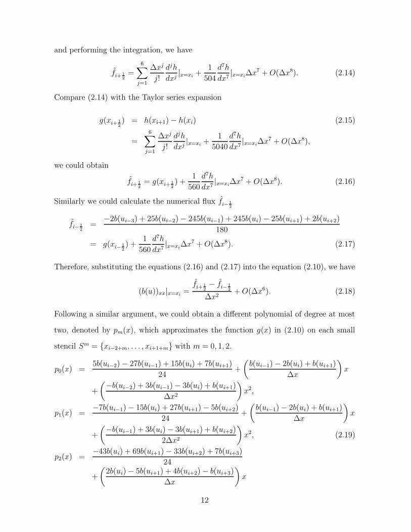
and performing the integration, we have
fi+ 12
=6∑
j=1
∆xj
j!
djh
dxj|x=xi
+1
504
d7h
dx7|x=xi
∆x7 + O(∆x8). (2.14)
Compare (2.14) with the Taylor series expansion
g(xi+ 12) = h(xi+1) − h(xi) (2.15)
=6∑
j=1
∆xj
j!
djh
dxj|x=xi
+1
5040
d7h
dx7|x=xi
∆x7 + O(∆x8),
we could obtain
fi+ 12
= g(xi+ 12) +
1
560
d7h
dx7|x=xi
∆x7 + O(∆x8). (2.16)
Similarly we could calculate the numerical flux fi− 12
fi− 12
=−2b(ui−3) + 25b(ui−2) − 245b(ui−1) + 245b(ui) − 25b(ui+1) + 2b(ui+2)
180
= g(xi− 12) +
1
560
d7h
dx7|x=xi
∆x7 + O(∆x8). (2.17)
Therefore, substituting the equations (2.16) and (2.17) into the equation (2.10), we have
(b(u))xx|x=xi=
fi+ 12− fi− 1
2
∆x2+ O(∆x6). (2.18)
Following a similar argument, we could obtain a different polynomial of degree at most
two, denoted by pm(x), which approximates the function g(x) in (2.10) on each small
stencil Sm = {xi−2+m, . . . , xi+1+m} with m = 0, 1, 2.
p0(x) =5b(ui−2) − 27b(ui−1) + 15b(ui) + 7b(ui+1)
24+
(
b(ui−1) − 2b(ui) + b(ui+1)
∆x
)
x
+
(
−b(ui−2) + 3b(ui−1) − 3b(ui) + b(ui+1)
∆x2
)
x2,
p1(x) =−7b(ui−1) − 15b(ui) + 27b(ui+1) − 5b(ui+2)
24+
(
b(ui−1) − 2b(ui) + b(ui+1)
∆x
)
x
+
(
−b(ui−1) + 3b(ui) − 3b(ui+1) + b(ui+2)
2∆x2
)
x2, (2.19)
p2(x) =−43b(ui) + 69b(ui+1) − 33b(ui+2) + 7b(ui+3)
24
+
(
2b(ui) − 5b(ui+1) + 4b(ui+2) − b(ui+3)
∆x
)
x
12
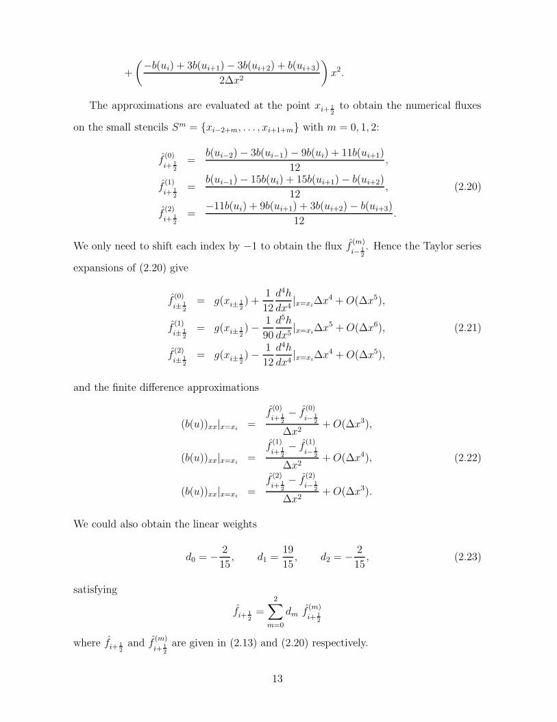
+
(
−b(ui) + 3b(ui+1) − 3b(ui+2) + b(ui+3)
2∆x2
)
x2.
The approximations are evaluated at the point xi+ 12
to obtain the numerical fluxes
on the small stencils Sm = {xi−2+m, . . . , xi+1+m} with m = 0, 1, 2:
f(0)
i+ 12
=b(ui−2) − 3b(ui−1) − 9b(ui) + 11b(ui+1)
12,
f(1)
i+ 12
=b(ui−1) − 15b(ui) + 15b(ui+1) − b(ui+2)
12, (2.20)
f(2)
i+ 12
=−11b(ui) + 9b(ui+1) + 3b(ui+2) − b(ui+3)
12.
We only need to shift each index by −1 to obtain the flux f(m)
i− 12
. Hence the Taylor series
expansions of (2.20) give
f(0)
i± 12
= g(xi± 12) +
1
12
d4h
dx4|x=xi
∆x4 + O(∆x5),
f(1)
i± 12
= g(xi± 12) −
1
90
d5h
dx5|x=xi
∆x5 + O(∆x6), (2.21)
f(2)
i± 12
= g(xi± 12) −
1
12
d4h
dx4|x=xi
∆x4 + O(∆x5),
and the finite difference approximations
(b(u))xx|x=xi=
f(0)
i+ 12
− f(0)
i− 12
∆x2+ O(∆x3),
(b(u))xx|x=xi=
f(1)
i+ 12
− f(1)
i− 12
∆x2+ O(∆x4), (2.22)
(b(u))xx|x=xi=
f(2)
i+ 12
− f(2)
i− 12
∆x2+ O(∆x3).
We could also obtain the linear weights
d0 = −2
15, d1 =
19
15, d2 = −
2
15, (2.23)
satisfying
fi+ 12
=2∑
m=0
dm f(m)
i+ 12
where fi+ 12
and f(m)
i+ 12
are given in (2.13) and (2.20) respectively.
13

2.2.1 A technique of treating negative weights
We could use the technique in [27] to treat the negative weights in (2.23). We split the
linear weights into two parts: positive and negative by defining
γ+m =
1
2(dm + θ|dm|), γ−
m = γ+m − dm, m = 0, 1, 2,
where θ = 3. Then we obtain
γ+0 =
2
15, γ+
1 =38
15, γ+
2 =2
15;
γ−0 =
4
15, γ−
1 =19
15, γ−
2 =4
15.
We scale them by
σ+ =2∑
m=0
γ+m =
42
15, σ− =
2∑
m=0
γ−m =
27
15, (2.24)
and obtain the linear weights of the two parts by γ±m = γ±
m/σ± with m = 0, 1, 2:
γ+0 =
1
21, γ+
1 =19
21, γ+
2 =1
21; (2.25)
γ−0 =
4
27, γ−
1 =19
27, γ−
2 =4
27. (2.26)
It is easy to check that
2∑
m=0
γ±m = 1, and dm = σ+γ+
m − σ−γ−m. (2.27)
2.2.2 The smoothness indicators and the nonlinear weights
To change the linear weights to nonlinear weights, we use the definition of the smoothness
function in the paper [15, 28]
βm =
2∑
l=1
∆x2l−1
∫ xi+1
xi
(
dl
dxlpm(x)
)2
dx, (2.28)
where the approximation polynomials pm(x) on the small stencils Sm = {xi−2+m, . . . , xi+1+m}
with m = 0, 1, 2 are given in (2.19), and obtain the smoothness indicators
β0 =13
12(b(ui−2) − 3b(ui−1) + 3b(ui) − b(ui+1))
2
14

+1
4(b(ui−2) − 5b(ui−1) + 7b(ui) − 3b(ui+1))
2,
β1 =13
12(b(ui−1) − 3b(ui) + 3b(ui+1) − b(ui+2))
2
+1
4(b(ui−1) − b(ui) − b(ui+1) + b(ui+2))
2, (2.29)
β2 =13
12(b(ui) − 3b(ui+1) + 3b(ui+2) − b(ui+3))
2
+1
4(−3b(ui) + 7b(ui+1) − 5b(ui+2) + b(ui+3))
2.
Here we perform the integration over the interval [xi, xi+1] to satisfy the symmetry
property of the parabolic equation, and the factor ∆x2l−1 in (2.28) is introduced to
remove any ∆x dependency in the final expression of the smoothness indicators in (2.29).
For the positive and negative linear weights γ±m in (2.25) and (2.26), we define the
nonlinear weights for the positive and negative groups ω±m respectively, denoted by ω±
m,
based on the same smoothness indicators βm given in (2.29)
ω±m =
ω±m
∑2l=0 ω±
l
, ω±m =
γ±m
(ε + βm)2, m = 0, 1, 2, (2.30)
where ε is to avoid the denominator to become zero, in this paper we take ε = 10−6. It
is easy to verify∑2
m=0 ω±m = 1.
2.2.3 The finite difference WENO scheme
Rewrite the positive and negative nonlinear weights in (2.30) together, we finally obtain
the nonlinear weights
ωm = σ+ω+m − σ−ω−
m (2.31)
with σ± given in (2.24), and the WENO approximation flux
fi+ 12
=
2∑
m=0
ωmf(m)
i+ 12
(2.32)
where f(m)
i+ 12
with m = 0, 1, 2 are given by (2.20).
Then the semi-discrete finite difference WENO scheme could be expressed as
dui(t)
dt=
fi+ 12− fi− 1
2
∆x2. (2.33)
15

2.2.4 Runge-Kutta time discretization
Up to now we have only considered spatial discretization, leaving the time variable
continuous. After the spatial discretization, the semi-discrete finite difference WENO
scheme is equivalent to the first-order ODE system:
du(t)
dt= L(u) (2.34)
where L(u) results from the right hand side of (2.33).
In this paper, we use the third-order TVD Runge-Kutta method [30] to solve (2.34),
which is given by
u(1) = un + ∆tL(un),
u(2) =3
4un +
1
4u(1) +
1
4∆tL(u(1)),
u(3) =1
3un +
2
3u(2) +
2
3∆tL(u(2)).
2.3 Analysis of the accuracy of the finite difference WENO
scheme
In order to achieve the objective of maintaining the same high order accuracy as in (2.18)
in smooth regions and non-oscillatory performance in regions where a discontinuity does
exist, we need to find out the accuracy requirement of the finite difference WENO scheme
(2.33).
Adding and subtracting∑2
m=0 dmf(m)
i+ 12
from (2.32) gives
fi+ 12
=2∑
m=0
dmf(m)
i+ 12
+2∑
m=0
(ωm − dm)f(m)
i+ 12
. (2.35)
Then we have
fi+ 12− fi− 1
2=
2∑
m=0
dmf(m)
i+ 12
−2∑
m=0
dmf(m)
i− 12
+2∑
m=0
(ω(+)m − dm)f
(m)
i+ 12
−2∑
m=0
(ω(−)m − dm)f
(m)
i− 12
,
(2.36)
16

where the superscript (+) or (−) on ωm indicate their use in the stencil of either fi+ 12
or
fi− 12. From equations (2.16), (2.17) and (2.18), the first two terms are
2∑
m=0
dmf(m)
i+ 12
−
2∑
m=0
dmf(m)
i− 12
= (b(u))xx|x=xi∆x2 + O(∆x8). (2.37)
We expand the last two terms in (2.36), substituting for f(m)
i± 12
from (2.21), and noticing
that∑2
m=0 dm =∑2
m=0 ωm = 1. Finally we obtain the necessary and sufficient conditions
to achieve sixth-order accuracy convergence
(ω(+)0 − ω
(−)0 − ω
(+)2 + ω
(−)2 ) = O(∆x4), (2.38)
(ωm − dm) = O(∆x3). (2.39)
Here we drop the superscript (±) because (2.38) and (2.39) constrain both the “+′′ and
“-” stencils. (2.39) gives us a simple set of criteria around which to design the nonlinear
weights ωm; while (2.38) is a difficult constraint to use in the design of the nonlinear
weights.
Therefore in order to satisfy the condition (2.39), we have to analyze the nonlinear
weights from (2.31). First we will consider the smoothness indicators βm with m = 0, 1, 2.
2.3.1 The analysis of the smoothness indicators
Expand the smoothness indicators βm (2.29) with m = 0, 1, 2 at the grid point xi
β0 = b2xx∆x4 + b2
xxbxxx∆x5 +1
3(4b2
xxx − bxxbxxxx)∆x6 + O(∆x7),
β1 = b2xx∆x4 + b2
xxbxxx∆x5 +2
3(2b2
xxx + bxxbxxxx)∆x6 + O(∆x7),
β2 = b2xx∆x4 + b2
xxbxxx∆x5 +1
3(4b2
xxx − bxxbxxxx)∆x6 + O(∆x7).
Therefore if
1. bxx 6= 0, we have βm = D(1 + O(∆x)) with m = 0, 1, 2;
2. bxx = 0, bxxx 6= 0, we have βm = D(1 + O(∆x)) with m = 0, 1, 2.
17
where D is a nonzero quantity independent of m (but may depend on the derivatives of
b(u(x)) and ∆x). From the previous analysis we have
βm = D(1 + O(∆x)), m = 0, 1, 2. (2.40)
2.3.2 The relationship between βm, γm and ωm
Through a Taylor expansion analysis, we conclude that βm = D(1 + O(∆xk−1)) is the
sufficient condition so that ωm = dm + O(∆xk−1) holds, where D is a nonzero quantity
independent of m (but may depend on ∆x).
Because of the Taylor expansion 1(1+x)2
= 1− 2x + 3x2 · · · near x = 0 and neglecting
ε, we could obtain
γ±m
(ε + βm)2=
γ±m
(D(1 + O(∆xk−1)))2=
γ±m
D2(1 + O(∆xk−1)).
From the definition of the nonlinear weights in (2.30) and∑2
m=0 γ±m = 1, we have
γ±m = ω±
m
(
2∑
l=0
γ±l
(ε + βl)2
)
(ε + βm)2,
= ω±m
(
1
D2(1 + O(∆xk−1))
)
(D(1 + O(∆xk−1)))2,
= ω±m + O(∆xk−1), m = 0, 1, 2. (2.41)
Thus through the previous analysis, the conditions (2.27), (2.40) and (2.41) imply that
the nonlinear weights defined in (2.30) and (2.31) are given by
ωm = dm + O(∆x), m = 0, 1, 2. (2.42)
Unfortunately, in this case the condition (2.39) is not satisfied, that is, we can not achieve
the sixth order accuracy by only using the nonlinear weights defined in (2.30) and (2.31).
2.3.3 Mapped nonlinear weights
To increase the accuracy of the nonlinear weights, we use the mapped function introduced
in [13]
gm(ω) =ω(dm + d2
m − 3dmω + ω2)
d2m + ω(1 − 2dm)
, m = 0, 1, 2. (2.43)
18

This function is monotonically increasing with a finite slope, gm(0) = 0, gm(1) = 1,
gm(dm) = dm, g′
m(dm) = 0 and g′′
m(dm) = 0. The mapped nonlinear weights are given by
αm = gm(ωm), m = 0, 1, 2, (2.44)
where dm and ωm are computed in (2.23), (2.30) and (2.31) respectively.
The mapped nonlinear weights are then defined as follows
ω(M)m =
αm∑2
m=0 αm
, m = 0, 1, 2. (2.45)
Hence the final form of the semi-discrete finite difference mapped WENO scheme is
dui(t)
dt=
fi+ 12− fi− 1
2
∆x2, (2.46)
with the approximation flux
fi+ 12
=2∑
m=0
ω(M)m f
(m)
i+ 12
, (2.47)
where f(m)
i+ 12
with m = 0, 1, 2 are given by (2.20).
By Taylor series approximation of the gm(ω) at dm and the condition (2.42) we have
αm = gm(dm) + g′
m(dm)(ωm − dm) +g
′′
m(dm)
2(ωm − dm)2 +
g′′′
m(dm)
6(ωm − dm)3 + · · ·
= dm +(ωm − dm)3
dm − d2m
+ · · · (2.48)
= dm + O(∆x3),
and then
ω(M)m = (dm + O(∆x3))(1 + O(∆x3)) = dm + O(∆x3), m = 0, 1, 2, (2.49)
because of∑2
m=0 dm = 1. Now the condition (2.39) is satisfied, therefore the mapped
WENO scheme (2.46) has the sixth order accuracy for smooth solutions and is non-
oscillatory near discontinuities as verified by numerical experiments given later.
19
2.4 Numerical results
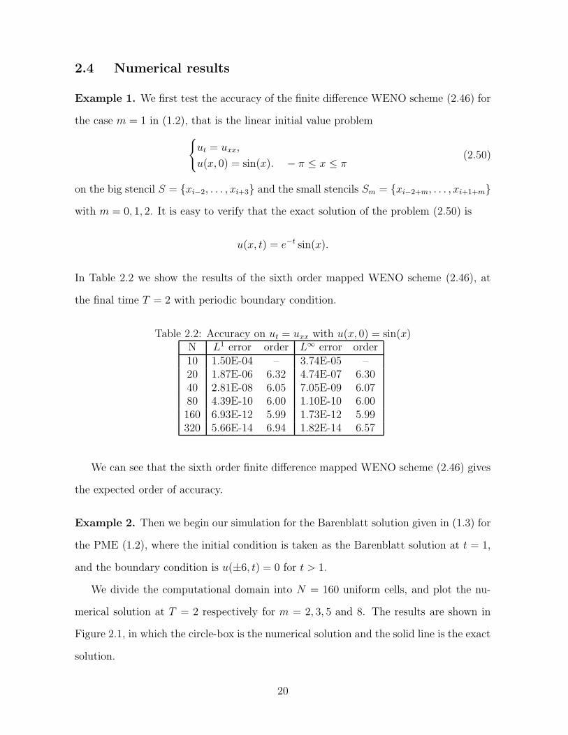
Example 1. We first test the accuracy of the finite difference WENO scheme (2.46) for
the case m = 1 in (1.2), that is the linear initial value problem
{
ut = uxx,
u(x, 0) = sin(x). − π ≤ x ≤ π(2.50)
on the big stencil S = {xi−2, . . . , xi+3} and the small stencils Sm = {xi−2+m, . . . , xi+1+m}
with m = 0, 1, 2. It is easy to verify that the exact solution of the problem (2.50) is
u(x, t) = e−t sin(x).
In Table 2.2 we show the results of the sixth order mapped WENO scheme (2.46), at
the final time T = 2 with periodic boundary condition.
Table 2.2: Accuracy on ut = uxx with u(x, 0) = sin(x)N L1 error order L∞ error order10 1.50E-04 – 3.74E-05 –20 1.87E-06 6.32 4.74E-07 6.3040 2.81E-08 6.05 7.05E-09 6.0780 4.39E-10 6.00 1.10E-10 6.00160 6.93E-12 5.99 1.73E-12 5.99320 5.66E-14 6.94 1.82E-14 6.57
We can see that the sixth order finite difference mapped WENO scheme (2.46) gives
the expected order of accuracy.
Example 2. Then we begin our simulation for the Barenblatt solution given in (1.3) for
the PME (1.2), where the initial condition is taken as the Barenblatt solution at t = 1,
and the boundary condition is u(±6, t) = 0 for t > 1.
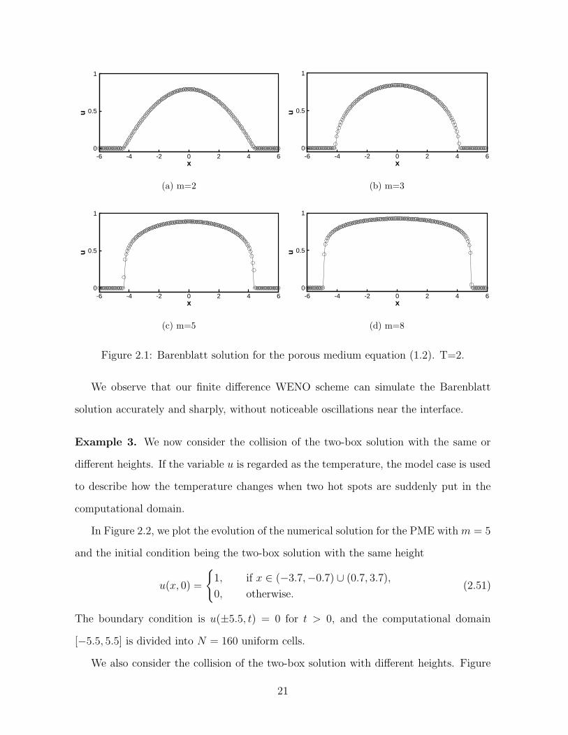
We divide the computational domain into N = 160 uniform cells, and plot the nu-
merical solution at T = 2 respectively for m = 2, 3, 5 and 8. The results are shown in
Figure 2.1, in which the circle-box is the numerical solution and the solid line is the exact
solution.
20
x
u
-6 -4 -2 0 2 4 60
0.5
1
(a) m=2
x
u
-6 -4 -2 0 2 4 60
0.5
1
(b) m=3
x
u
-6 -4 -2 0 2 4 60
0.5
1
(c) m=5
x
u-6 -4 -2 0 2 4 6
0
0.5
1
(d) m=8
Figure 2.1: Barenblatt solution for the porous medium equation (1.2). T=2.
We observe that our finite difference WENO scheme can simulate the Barenblatt
solution accurately and sharply, without noticeable oscillations near the interface.
Example 3. We now consider the collision of the two-box solution with the same or
different heights. If the variable u is regarded as the temperature, the model case is used
to describe how the temperature changes when two hot spots are suddenly put in the
computational domain.
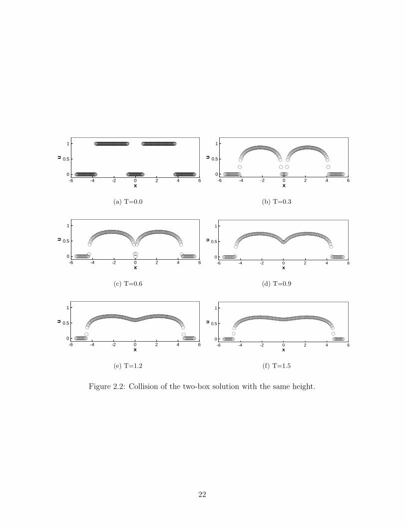
In Figure 2.2, we plot the evolution of the numerical solution for the PME with m = 5
and the initial condition being the two-box solution with the same height
u(x, 0) =
{
1, if x ∈ (−3.7,−0.7) ∪ (0.7, 3.7),
0, otherwise.(2.51)
The boundary condition is u(±5.5, t) = 0 for t > 0, and the computational domain
[−5.5, 5.5] is divided into N = 160 uniform cells.
We also consider the collision of the two-box solution with different heights. Figure
21
x
u
-6 -4 -2 0 2 4 60
0.5
1
(a) T=0.0
x
u
-6 -4 -2 0 2 4 60
0.5
1
(b) T=0.3
x
u
-6 -4 -2 0 2 4 60
0.5
1
(c) T=0.6
x
u
-6 -4 -2 0 2 4 60
0.5
1
(d) T=0.9
x
u
-6 -4 -2 0 2 4 60
0.5
1
(e) T=1.2
x
u
-6 -4 -2 0 2 4 60
0.5
1
(f) T=1.5
Figure 2.2: Collision of the two-box solution with the same height.
22
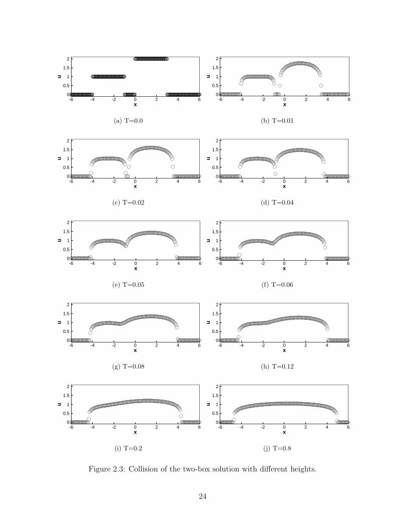
2.3 is the evolution of the numerical solution for the PME with m = 6. The initial
condition is
u(x, 0) =
1, if x ∈ (−4,−1),
2, if x ∈ (0, 3),
0, otherwise.
(2.52)
The boundary condition is u(±6, 0) = 0 for t > 0, and the computational domain is
divided into N = 160 uniform cells.
From Figures 2.2 and 2.3, we could see that whether the heights of the two boxes
in the initial condition are the same or not, the two-box solutions first move outward
independently before the collision, then they join each other to make the temperature
smooth, and finally the solution becomes almost constant in the common support, agree-
ing with the results in [32].
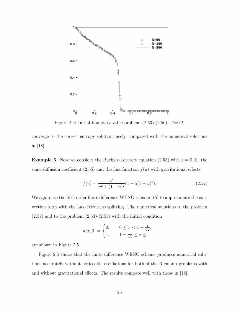
Example 4. Next we consider the scalar convection-diffusion Buckley-Leverett equation
introduced in [18]
ut + f(u)x = ε(ν(u)ux)x, εν(u) ≥ 0. (2.53)
This is a prototype model for oil reservoir simulations (two-phase flow). In our test we
take ε = 0.01, f(u) to have a s-shaped form
f(u) =u2
u2 + (1 − u)2, (2.54)
and
ν(u) = 4u(1 − u). (2.55)
The initial function is
u(x, 0) =
{
1 − 3x, 0 ≤ x ≤ 13,
0, 13
< x ≤ 1.(2.56)
and the boundary condition is u(0, t) = 1.
With the Lax-Friedrichs flux splitting, we apply the fifth order finite difference WENO
scheme [15] to approximate the convection term. The numerical solution computed for
different number of grid points is shown in Figure 2.4. The numerical results seem to
23
x
u
-6 -4 -2 0 2 4 60
0.5
1
1.5
2
(a) T=0.0
x
u
-6 -4 -2 0 2 4 60
0.5
1
1.5
2
(b) T=0.01
x
u
-6 -4 -2 0 2 4 60
0.5
1
1.5
2
(c) T=0.02
x
u
-6 -4 -2 0 2 4 60
0.5
1
1.5
2
(d) T=0.04
x
u
-6 -4 -2 0 2 4 60
0.5
1
1.5
2
(e) T=0.05
x
u
-6 -4 -2 0 2 4 60
0.5
1
1.5
2
(f) T=0.06
x
u
-6 -4 -2 0 2 4 60
0.5
1
1.5
2
(g) T=0.08
x
u
-6 -4 -2 0 2 4 60
0.5
1
1.5
2
(h) T=0.12
x
u
-6 -4 -2 0 2 4 60
0.5
1
1.5
2
(i) T=0.2
x
u
-6 -4 -2 0 2 4 60
0.5
1
1.5
2
(j) T=0.8
Figure 2.3: Collision of the two-box solution with different heights.
24
0 0.2 0.4 0.6 0.8 10
0.2
0.4
0.6
0.8
1
N=50N=100N=800
Figure 2.4: Initial-boundary value problem (2.53)-(2.56). T=0.2.
converge to the correct entropy solution nicely, compared with the numerical solutions
in [18].
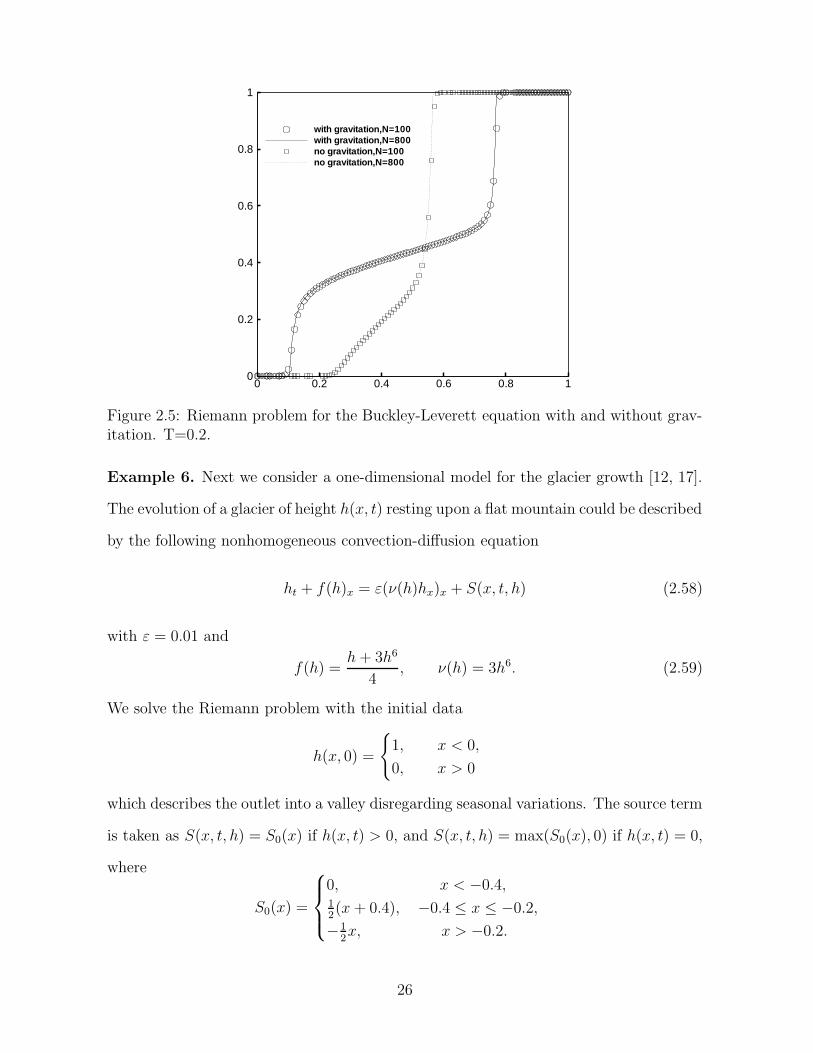
Example 5. Now we consider the Buckley-Leverett equation (2.53) with ε = 0.01, the
same diffusion coefficient (2.55) and the flux function f(u) with gravitational effects
f(u) =u2
u2 + (1 − u)2(1 − 5(1 − u)2). (2.57)
We again use the fifth order finite difference WENO scheme [15] to approximate the con-
vection term with the Lax-Friedrichs splitting. The numerical solutions to the problem
(2.57) and to the problem (2.53)-(2.55) with the initial condition
u(x, 0) =
{
0, 0 ≤ x < 1 − 1√2,
1, 1 − 1√2≤ x ≤ 1
are shown in Figure 2.5.
Figure 2.5 shows that the finite difference WENO scheme produces numerical solu-
tions accurately without noticeable oscillations for both of the Riemann problems with
and without gravitational effects. The results compare well with those in [18].
25
0 0.2 0.4 0.6 0.8 10
0.2
0.4
0.6
0.8
1
with gravitation,N=100with gravitation,N=800no gravitation,N=100no gravitation,N=800
Figure 2.5: Riemann problem for the Buckley-Leverett equation with and without grav-itation. T=0.2.
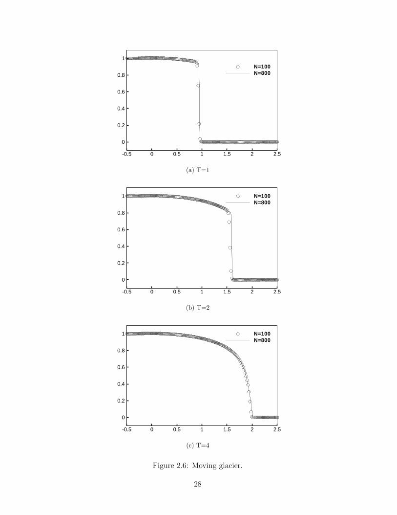
Example 6. Next we consider a one-dimensional model for the glacier growth [12, 17].
The evolution of a glacier of height h(x, t) resting upon a flat mountain could be described
by the following nonhomogeneous convection-diffusion equation
ht + f(h)x = ε(ν(h)hx)x + S(x, t, h) (2.58)
with ε = 0.01 and
f(h) =h + 3h6
4, ν(h) = 3h6. (2.59)
We solve the Riemann problem with the initial data
h(x, 0) =
{
1, x < 0,
0, x > 0
which describes the outlet into a valley disregarding seasonal variations. The source term
is taken as S(x, t, h) = S0(x) if h(x, t) > 0, and S(x, t, h) = max(S0(x), 0) if h(x, t) = 0,
where
S0(x) =
0, x < −0.4,12(x + 0.4), −0.4 ≤ x ≤ −0.2,
−12x, x > −0.2.
26

The numerical solutions are shown in Figure 2.6 for different numbers of grid points at
different times. They seem to converge well with grid refinement and agree well with the
results in [17, 18].
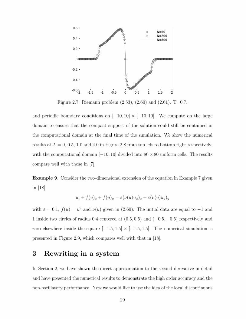
Example 7. In this test we consider an example of strongly degenerate parabolic
convection-diffusion equation presented in [18]
ut + f(u)x = ε(ν(u)ux)x, εν(u) ≥ 0.
We take ε = 0.1, f(u) = u2 and
ν(u) =
{
0, |u| ≤ 0.25,
1, |u| > 0.25.(2.60)
Therefore the equation is hyperbolic when u ∈ [−0.25, 0.25] and parabolic elsewhere.
We solve the problem with the initial function
u(x, 0) =
1, − 1√2− 0.4 < x < − 1√
2+ 0.4,
−1, 1√2− 0.4 < x < 1√
2+ 0.4,
0, otherwise.
(2.61)
The numerical simulations for different numbers of gird points are presented in Figure
2.7, which agree well with the results in [18].
Example 8. Our finite difference WENO scheme (2.46) could also be easily extended
to higher dimension, since derivatives in each dimension can be approximated using the
one-dimensional point values in that dimension. Here we present a numerical simulation
for the two-dimensional porous medium equation
ut = (u2)xx + (u2)yy. (2.62)
with the initial condition u0(x, y) given by two bumps
u0(x, y) =
e−1
6−(x−2)2−(y+2)2 , (x − 2)2 + (y + 2)2 < 6,
e−1
6−(x+2)2−(y−2)2 , (x + 2)2 + (y − 2)2 < 6,
0, otherwise
(2.63)
27
-0.5 0 0.5 1 1.5 2 2.5
0
0.2
0.4
0.6
0.8
1
N=100N=800
(a) T=1
-0.5 0 0.5 1 1.5 2 2.5
0
0.2
0.4
0.6
0.8
1 N=100N=800
(b) T=2
-0.5 0 0.5 1 1.5 2 2.5
0
0.2
0.4
0.6
0.8
1 N=100N=800
(c) T=4
Figure 2.6: Moving glacier.
28
-2 -1.5 -1 -0.5 0 0.5 1 1.5 2-0.6
-0.4
-0.2
0
0.2
0.4
0.6N=60N=200N=800
Figure 2.7: Riemann problem (2.53), (2.60) and (2.61). T=0.7.
and periodic boundary conditions on [−10, 10] × [−10, 10]. We compute on the large
domain to ensure that the compact support of the solution could still be contained in
the computational domain at the final time of the simulation. We show the numerical
results at T = 0, 0.5, 1.0 and 4.0 in Figure 2.8 from top left to bottom right respectively,
with the computational domain [−10, 10] divided into 80× 80 uniform cells. The results
compare well with those in [7].
Example 9. Consider the two-dimensional extension of the equation in Example 7 given
in [18]
ut + f(u)x + f(u)y = ε(ν(u)ux)x + ε(ν(u)uy)y
with ε = 0.1, f(u) = u2 and ν(u) given in (2.60). The initial data are equal to −1 and
1 inside two circles of radius 0.4 centered at (0.5, 0.5) and (−0.5,−0.5) respectively and
zero elsewhere inside the square [−1.5, 1.5] × [−1.5, 1.5]. The numerical simulation is
presented in Figure 2.9, which compares well with that in [18].
3 Rewriting in a system
In Section 2, we have shown the direct approximation to the second derivative in detail
and have presented the numerical results to demonstrate the high order accuracy and the
non-oscillatory performance. Now we would like to use the idea of the local discontinuous
29

(a) T=0. (b) T=0.5
(c) T=1.0 (d) T=4.0
Figure 2.8: The numerical solution of the porous medium equation in 2D.
-1.5 -1 -0.5 0 0.5 1 1.5
Figure 2.9: Degenerate parabolic problem-solution at time T=0.5 on a 60 × 60 grid.
30
Galerkin method [10], to first rewrite the equation (1.1) as a nonlinear system of first
order equations
ut = vx, (3.1)
v = b(u)x (3.2)
and then to solve the two first order equations respectively using the fifth order finite
difference WENO method for conservation laws [15]. In order to make the final effective
stencil smaller, we use a right-biased stencil for (3.1) followed by a left-biased stencil for
(3.2).
3.1 Approximation to two first derivatives
3.1.1 Approximation to the second equation (3.2)
Based on the left-biased big stencil S = {xi−2, . . . , xi+2}, assuming the grid is uniform,
i.e. ∆x = xi+1 − xi is a constant, we first solve the equation (3.2) using the finite
difference approximation and writing it in a conservative form
vi =gi+ 1
2− gi− 1
2
∆x. (3.3)
Given the point values of the function b(u(x)), the problem we face now is to find a
numerical flux function
gi+ 12
= g(ui−2, . . . , ui+2) (3.4)
such that the flux difference approximates the first order derivative b(u(x))x at x = xi
to fifth order accuracy
gi+ 12− gi− 1
2
∆x= (b(u))x|x=xi
+ O(∆x5). (3.5)
This is the standard problem for solving conservation laws [15]. We therefore only list
the results here.
We could obtain the flux gi+ 12
based on the big stencil as
gi+ 12
=2b(ui−2) − 13b(ui−1) + 47b(ui) + 27b(ui+1) − 3b(ui+2)
60. (3.6)
31
Similarly, we could evaluate the three different fluxes
g(0)
i+ 12
=2b(ui−2) − 7b(ui−1) + 11b(ui)
6,
g(1)
i+ 12
=−b(ui−1) + 5b(ui) + 2b(ui+1)
6, (3.7)
g(2)
i+ 12
=2b(ui) + 5b(ui+1) − b(ui+2)
6,
which are based on the three small stencils Sm = {xi−2+m, xi−1+m, xi+m} with m = 0, 1, 2
respectively.
The linear weights dm with m = 0, 1, 2 are given by
d0 =1
10, d1 =
3
5, d2 =
3
10,
satisfying gi+ 12
=∑2
m=0 dmg(m)
i+ 12
and the consistence condition∑2
m=0 dm = 1. The
smoothness indicators are given by
β0 =13
12(b(ui−2) − 2b(ui−1) + b(ui))
2 +1
4(b(ui−2) − 4b(ui−1) + 3b(ui))
2,
β1 =13
12(b(ui−1) − 2b(ui) + b(ui+1))
2 +1
4(b(ui−1) − b(ui+1))
2, (3.8)
β2 =13
12(b(ui) − 2b(ui+1) + b(ui+2))
2 +1
4(3b(ui) − 4b(ui+1) + b(ui+2))
2.
Therefore we discretize the equation (3.2) on the left-biased big stencil S = {xi−2, . . . , xi+2}
in the form (3.3), where the flux is constructed as follows
gi+ 12
=
2∑
m=0
ωmg(m)
i+ 12
(3.9)
with g(m)
i+ 12
given in (3.7) and the nonlinear weights defined by
ωm =αm
∑2j=0 αj
, αm =dm
(ε + βm)2, m = 0, 1, 2. (3.10)
Here ε is again taken as 10−6. The smoothness indicators βm with m = 0, 1, 2 are given
in (3.8).
32

3.1.2 Approximation to the first equation (3.1)
In Section 3.1.1, we have obtained the point values of the function v(x) in (3.2). We
can use the previous reconstruction again to get the numerical flux fi+ 12
for solving the
equation (3.1) based on the right-biased big stencil S = {xi−1, . . . , xi+3}, written in the
form
dui(t)
dt=
fi+ 12− fi− 1
2
∆x. (3.11)
Following a similar argument as in the previous section, we could obtain the fluxes
f(0)
i+ 12
=−vi−1 + 5vi−1 + 2vi
6,
f(1)
i+ 12
=2vi + 5vi+1 − vi+2
6, (3.12)
f(2)
i+ 12
=11vi − 7vi+2 + 2vi+3
6,
the linear weights
d0 =3
10, d1 =
3
5, d2 =
1
10,
and the nonlinear weights defined by
ωm =αm
∑2j=0 αj
, αm =dm
(ε + βm)2, m = 0, 1, 2, (3.13)
based on the three small stencils Sm = {xi−1+m, xi+m, xi+1+m} with m = 0, 1, 2 respec-
tively. Here the smooth indicators βm are
β0 =13
12(vi−1 − 2vi + vi+1)
2 +1
4(vi−1 − 4vi + 3vi+1)
2,
β1 =13
12(vi − 2vi+1 + vi+2)
2 +1
4(vi − vi+2)
2, (3.14)
β2 =13
12(vi+1 − 2vi+2 + vi+3)
2 +1
4(3vi+1 − 4vi+2 + vi+3)
2.
Finally on the right-biased big stencil S = {xi−1, . . . , xi+3} we obtain the numerical
flux for the fifth finite difference WENO scheme (3.11)
fi+ 12
=2∑
m=0
ωmf(m)
i+ 12
(3.15)
where ωm and f(m)
i+ 12
are given in (3.13) and (3.12) respectively.
33

Table 3.1: Accuracy on ut = uxx with u(x, 0) = sin(x)N L1 error order L∞ error order10 6.05E-03 – 2.63E-03 –20 1.13E-04 5.74 4.25E-05 5.9540 1.78E-06 5.99 7.08E-07 5.9180 2.62E-08 6.08 1.12E-08 5.98160 3.95E-10 6.05 1.73E-10 6.01320 4.74E-12 6.38 2.74E-12 5.98
3.2 Numerical results for the PME
For the time discretization, we still use the same third order TVD Runge-Kutta method
given in Section 2.2.4.
Example 10. Similarly we first test the accuracy of the finite difference WENO scheme
constructed in (3.3) and (3.11) for the case m = 1 in (1.2), that is the linear problem
with the smooth initial condition (2.50). Table 3.1 shows the results at the final time
T = 2 with periodic boundary condition.
We could see that this second WENO method also achieves sixth order accuracy,
however its error magnitude is larger than that of the first WENO method in the previous
section on the same mesh. Notice that the second WENO method also involves more
computation and has a larger effective stencil.
Example 11. Now we compute the Barenblatt solution given in (1.3) of the PME (1.2),
with the initial condition taken as the Barenblatt solution at t = 1, and the boundary
condition u(±6, t) = 0 for t > 1.
Dividing the computational domain into N = 160 uniform cells, we plot the numerical
solution at T = 2 respectively for m = 2, 3, 5 and 8. The circle-box is the numerical
solution and the solid line is the exact solution.
We could observe that by rewriting the PME as a system, the finite difference WENO
scheme can also simulate the Barenblatt solution accurately and sharply, without no-
ticeable oscillations near the interface.
34

x
u
-6 -4 -2 0 2 4 60
0.5
1
(a) m=2
x
u
-6 -4 -2 0 2 4 60
0.5
1
(b) m=3
x
u
-6 -4 -2 0 2 4 60
0.5
1
(c) m=5
x
u-6 -4 -2 0 2 4 6
0
0.5
1
(d) m=8
Figure 3.1: Numerical results by rewriting in a system. T=2.
We have also applied the second WENO scheme in this section to Examples 3 to 9
in the previous section, obtaining equally good non-oscillatory solutions. We will not
present the results here to save space.
4 Concluding remarks
In this paper we consider two different formulations of WENO schemes for approximating
possibly degenerate parabolic equations. The first formulation approximates directly
the second derivative term using a conservative flux difference and the second approach
applies the WENO procedure to two first order equations using the idea of the local
discontinuous Galerkin method. Both of the numerical methods could achieve high order
accuracy and can simulate discontinuous solutions without oscillations. Comparing Table
2.2 and Table 3.1, we observe that even though both of them could achieve sixth order
accuracy, the first method has a smaller error magnitude on the same mesh.
35
References
[1] D. Aregba-Driollet, R. Natalini, and S. Tang, Explicit diffusive kinetic schemes for
nonlinear degenerate parabolic systems, Mathematics of Computation, 73 (2004),
63-94.
[2] D.G. Aronson, The porous medium equation, in Nonlinear Diffusion Problems, Lec-
ture Notes in Mathematics, Springer Berlin, 1224 (1986), 1-46.
[3] D. Balsara and C.-W. Shu, Monotonicity preserving weighted essentially non-
oscillatory schemes with increasingly high order of accuracy, Journal of Compu-
tational Physics, 160 (2000), 405-452.
[4] G.I. Barenblatt, On self-similar motions of compressible fluid in a porous medium,
Prikl. Mat. Mekh., 16 (1952), 679-698 (in Russian).
[5] A.E. Berger, H. Brezis and J.C. Rogers, A numerical method for solving the problem
ut − ∆f(u) = 0, RAIRO Numerical Analysis, 13 (1979), 297-312.
[6] E. Carlini, R. Ferretti and G. Russo, A weighted essentially nonoscillatory, large
time-step scheme for Hamilton-Jacobi equations, SIAM Journal on Scientific Com-
puting, 27 (2005), 1071-1091.
[7] F. Cavalli, G. Naldi, G. Puppo and M. Semplice, High order relaxation schemes for
nonlinear degenerate diffusion problems, SIAM Journal on Numerical Analysis, 45
(2007), 2098-2119.
[8] C.-S. Chou and C.-W. Shu, High order residual distribution conservative finite dif-
ference WENO schemes for steady state problems on non-smooth meshes, Journal
of Computational Physics, 214 (2006), 698-724.
36
[9] C.-S. Chou and C.-W. Shu, High order residual distribution conservative finite differ-
ence WENO schemes for convection-diffusion steady state problems on non-smooth
meshes, Journal of Computational Physics, 224 (2007), 992-1020.
[10] B. Cockburn and C.-W. Shu, The local discontinuous Galerkin method for time-
dependent convection-diffusion systems, SIAM Journal on Numerical Analysis, 35
(1998), 2440-2463.
[11] S. Evje and K. H. Karlsen, Viscous splitting approximation of mixed hyperbolic-
parabolic convection-diffusion equations, Numerische Mathematik, 83(1999), 107-
137.
[12] A.C. Flower, Glaciers and ice sheets, in The Mathematics of Model for Clima-
tology and Environment, edited by J.I. Diaz, NATO ASI Series, Springer-Verlag,
Berlin/New York, 48 (1996), 302-336.
[13] A.K. Henrick, T.D. Aslam and J.M. Powers, Mapped weighted essentially non-
oscillatory schemes: Achieving optimal order near critical points, Journal of Com-
putational Physics, 207 (2005), 542-567.
[14] W. Jager and J. Kacur, Solution of porous medium type systems by linear approxi-
mation schemes, Numerische Mathematik, 60 (1991), 407-427.
[15] G. Jiang and C.-W. Shu, Efficient implementation of weighted ENO schemes, Jour-
nal of Computational Physics, 126 (1996), 202-228.
[16] J. Kacur, A. Handlovicova, and M. Kacurova, Solution of nonlinear diffusion prob-
lems by linear approximation schemes, SIAM Journal on Numerical Analysis, 30
(1993), 1703-1722.
[17] K.H. Karlsen and K.A. Lie, An unconditionally stable splitting for a class of non-
linear parabolic equations, IMA Journal of Numerical Analysis, 19 (1999), 609-635.
37

[18] A. Kurganov and E. Tadmor, New high-resolution central schemes for nonlinear
conservation laws and convection-diffusion equations, Journal of Computational
Physics, 160 (2000), 241-282.
[19] X.-D. Liu, S. Osher and T. Chan, Weighted essentially non-oscillatory schemes,
Journal of Computational Physics, 115 (1994), 200-212.
[20] Y. Liu, C.-W. Shu and M. Zhang, On the positivity of linear weights in WENO
approximations, Acta Mathematicae Applicatae Sinica, 25 (2009), 503-538.
[21] E. Magenes, R.H. Nochetto, and C. Verdi, Energy error estimates for a linear
scheme to approximate nonlinear parabolic problems, RAIRO Mathematical Mod-
elling and Numerical Analysis, 21 (1987), 655-678.
[22] M. Muskat, The flow of homogeneous fluids through porous media, McGraw-Hill
Book Co., New York, 1937.
[23] R.H. Nochetto, A. Schmidt and C. Verdi, A posteriori error estimation and adap-
tivity for degenerate parabolic problems, Mathematics of Computation, 69 (2000),
1-24.
[24] R.H. Nochetto, and C. Verdi, Approximation of degenerate parabolic problems using
numerical integration, SIAM Journal on Numerical Analysis, 25 (1988), 784-814.
[25] I.S. Pop and W. Yong, A numerical approach to degenerate parabolic equations,
Numerische Mathematik, 92 (2002), 357-381.
[26] K. Sebastian and C.-W. Shu, Multi domain WENO finite difference method with
interpolation at sub-domain interfaces, Journal of Scientific Computing, 19 (2003),
405-438.
[27] J. Shi, C. Hu and C.-W. Shu, A technique of treating negative weights in WENO
schemes, Journal of Computational Physics, 175 (2002), 108-127.
38
[28] C.-W. Shu, Essentially non-oscillatory and weighted essentially non-oscillatory
schemes for hyperbolic conservation laws, in Advanced Numerical Approximation
of Nonlinear Hyperbolic Equations, B. Cockburn, C. Johnson, C.-W. Shu and E.
Tadmor (Editor: A. Quarteroni), Lecture Notes in Mathematics, Springer, 1697
(1998), 325-432.
[29] C.-W. Shu, High order weighted essentially non-oscillatory schemes for convection
dominated problems, SIAM Review, 51 (2009), 82-126.
[30] C.-W. Shu and S. Osher, Efficient implementation of essentially non-oscillatory
shock-capturing schemes, Journal of Computational Physics, 77 (1988), 439-471.
[31] Ya.B. Zel’dovich and A.S. Kompaneetz, Towards a theory of heat conduction with
thermal conductivity depending on the temperature, in Collection of papers dedicated
to 70th Anniversary of A.F. Ioffe, Izd. Akad. Nauk SSSR, Moscow, 1950, 61-72.
[32] Q. Zhang and Z. Wu, Numerical simulation for porous medium equation by local
discontinuous Galerkin finite element method, Journal of Scientific Computing, 38
(2009), 127-148.
39