Implementation of the

Adaptive Pure Pursuit Controller

Team 1712

1

Table Of Contents

Abstract 3

Overview 4

Odometry 4

Path Generation 5 Injecting Points 5 Smoothing 6 Distances Between Points 6 Curvature of Path 7 Velocities 8

Following the Path 10 Closest Point 10 Lookahead Point 10 Curvature of Arc 11 Wheel Velocities 14 Controlling Wheel Velocities 15 Tuning 16 Stopping 17

On the Importance of Visualizations 17

Conclusion 18

References 19

2

Abstract The adaptive pure pursuit controller makes a robot follow a path quickly, smoothly, and

accurately. Unlike motion profiling which gives target wheel velocities based on how much time

has elapsed, pure pursuit gives targets velocities based on where the robot is in relation to the

path it wants to follow. This makes it very robust: if the controller’s parameters are poorly

tuned, the robot starts in the wrong place, the carpet is bumpy, or even if it hits other robots,

the robot will be able to correct itself to follow the path and get to the goal.

We would like to thank the authors at Carnegie Mellon University for the general overview of

the algorithm, which can be found here:

https://www.ri.cmu.edu/pub_files/pub3/coulter_r_craig_1992_1/coulter_r_craig_1992_1.pdf

We highly suggest reading it as a supplement to this whitepaper.

Overview The heart of the pure pursuit controller is directing the robot to travel along an arc from the

current location to the goal point. This goal point is called the lookahead point and it is a point

on the path that is the lookahead distance from the robot. As the robot moves along the path,

it aims for the lookahead point, which moves down the path with the robot. In this way, the

robot can be considered to “pursue” the lookahead point. This action is analogous to how a

human driver looks at a point down the road and aims towards that point.

1

There are three parts to implementing the pure pursuit controller: odometry, generating the

path, and following the path. Let’s start with odometry.

1 https://www.mathworks.com/help/robotics/ug/pure-pursuit-controller.html

3

Odometry Odometry is finding the robot’s XY location. The simplest way of doing this is to use encoders

attached to the drive wheels to measure how far the robot moved, and to use the gyro to

measure in which direction. By repeating this math 50 times per second, the robot gets a fair

approximation of its current location. The math is as follows:

istance (change in lef t encoder value change in right encoder value)/2d = +

location = distance osine(robot angle)x + * c

location = distance ine(robot angle)y + * s

This gives the location of the robot relative to its starting location, which by default is (0, 0). If

you change the starting location to be the robot’s starting location on the field, then the

calculated location will be field-centric (relative to the field). When running paths one after

another, using field-centric coordinates can reduce buildup of errors caused by the robot not

stopping precisely , as the robot will still know where it is on the field and can correct itself 2

during the next path. Field-centric coordinates can also make drawing paths more intuitive.

You could also use other forms of odometry, such as vision or LIDAR (which are not discussed in

this paper).

Path Generation A path is a series of XY coordinates (called waypoints) which are created by first outlining a few

waypoints for the robot to follow. The software then injects more waypoints into the path and

smooths the path. Then the following information is calculated and stored for every waypoint

in the path:

● Distance that point is along the path

● Target velocity of the robot at that point

● Curvature of the path at that point

When creating a path, the user also sets the maximum velocity and acceleration of the robot.

Here is a visualization of creating waypoints for a path:

2 The pure pursuit controller is designed to follow paths, not stop precisely at the end of them. It still does very well though.

4

Injecting points

Having closely spaced points increases the accuracy of the velocity setpoints and curvature

measurements. Additionally, the smoothing algorithm we use works best with lots of points.

Our injection algorithm calculates how many evenly spaced points would fit within each line

segment of the path (including the start point, excluding the end point), then inserts them

along the segment. It does this for every segment in the path. When it gets to the end, it has

still not added the endpoint of the path, so it adds it to the list of points. Here is a pseudocode

version of this algorithm:

spacing = desired distance between points

new_points = array to put new points into

● For every line segment in the path:

○ vector = end_point - start_point

○ num_points_that_fit = Math.ceil(vector.magnitude() / spacing)

○ vector = vector.normalize() * spacing

○ for (i = 0; i<num_points_that_fit; i++):

■ Add (start_point + vector * i) to new_points

● Add the very last point in the path to new_points

We have found that a spacing of 6” works fine. If you have a different method of inserting

points, then go for it.

Smoothing

To smooth the path, we use an algorithm borrowed from Team 2168. The algorithm takes in a

2D array of XY coordinates and returns a smoother version of the coordinates. It takes in three

parameters: weight_data (which we call a), weight_smooth (b), and tolerance. The amount this

algorithm smooths depends on the spacing between the points and the values of a, b, and

tolerance. A larger b means a smoother path. We have found a value of b between 0.75 and

0.98 to work well, with a set to 1 - b and tolerance = 0.001. You can tune b on a per-path basis,

5

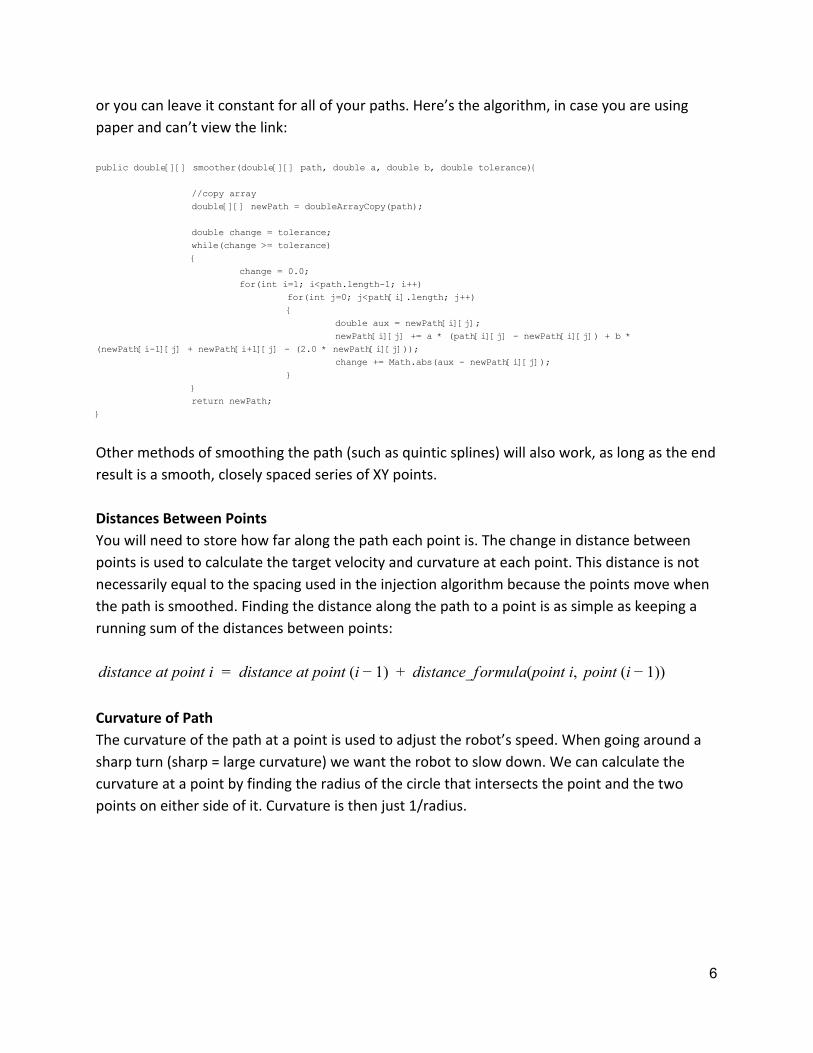
or you can leave it constant for all of your paths. Here’s the algorithm, in case you are using

paper and can’t view the link:

public double[][] smoother(double[][] path, double a, double b, double tolerance){

//copy array

double[][] newPath = doubleArrayCopy(path);

double change = tolerance;

while(change >= tolerance)

{

change = 0.0;

for(int i=1; i<path.length-1; i++)

for(int j=0; j<path[i].length; j++)

{

double aux = newPath[i][j];

newPath[i][j] += a * (path[i][j] - newPath[i][j]) + b *

(newPath[i-1][j] + newPath[i+1][j] - (2.0 * newPath[i][j]));

change += Math.abs(aux - newPath[i][j]);

}

}

return newPath;

}

Other methods of smoothing the path (such as quintic splines) will also work, as long as the end

result is a smooth, closely spaced series of XY points.

Distances Between Points

You will need to store how far along the path each point is. The change in distance between

points is used to calculate the target velocity and curvature at each point. This distance is not

necessarily equal to the spacing used in the injection algorithm because the points move when

the path is smoothed. Finding the distance along the path to a point is as simple as keeping a

running sum of the distances between points:

istance at point i distance at point (i ) distance_formula(point i, point (i ))d = − 1 + − 1

Curvature of Path

The curvature of the path at a point is used to adjust the robot’s speed. When going around a

sharp turn (sharp = large curvature) we want the robot to slow down. We can calculate the

curvature at a point by finding the radius of the circle that intersects the point and the two

points on either side of it. Curvature is then just 1/radius.

6

Derivation: (method 2 of https://www.qc.edu.hk/math/Advanced%20Level/circle%20given%203%20points.htm)

Given three points P(x1, y1), Q(x2, y2), and R(x3, y3), we are trying to find the circle with center

C(a, b) and radius r that intersects P, Q, and R. We can write r = |PC| = |QC| = |RC|. The

solution to this is:

.5 x y x y )/(x x )k1 = 0 * ( 12 + 1

2 − 22 − 2

21 − 2

y y )/(x x )k2 = ( 1 − 2 1 − 2

.5 x 2 )/(x )b = 0 * ( 22 − * x2 * k1 + y2

2 − x32 + 2 * x3 * k1 − y3

23 * k2 − y3 + y2 − x2 * k2

a = k1 − k2 * b

r = √(x ) y )1 − a 2 + ( 1 − b 2

urvature /rc = 1

This formula has the following edge cases:

If you get a divide-by-zero error. To fix this, add a sufficiently small value (0.001) to .x1 = x2 x1

The formula then gives a very close approximation without any errors.

If the answer is NaN, this means the radius is ∞ , the curvature is 0, and the path is a straight

line.

To find the curvature at each point along the path, we take each point and the points on either

side of it and plug them into this formula. For the start and end points, which do not have a

point on either side, the curvature is 0.

7

Velocities

Part 1: Maximum velocities

Each point on the path will have a target velocity the robot tries to reach. The robot uses the

target velocity of the point closest to it when calculating the target left and right wheel speeds.

When calculating the target velocity for a point we take into account the curvature at the point

so the robot slows down around sharp turns. The maximum velocity defined for the path is also

taken into account. Each point’s velocity is set to the minimum of

, where k is a constant around 1-5, based on howpath max velocity, k / curvature at point)(

slow you want the robot to go around turns. This reduces the speed of the robot around turns,

while making sure the robot’s target speed is never above the maximum. The following diagram

demonstrates what a graph of each point’s target velocity might look like for a certain path:

Part 2: Acceleration limits

As our robot travels along the path, we want it to follow the velocity setpoints, but also obey a

maximum acceleration. Instead of going from 0 to 100 instantaneously, we want the target

velocities to smoothly change. We want to take the blue target velocities line calculated above

and turn it into the orange line below: 3

This produces a problem. The robot’s target velocity is

based on which point it is closest to, and in this graph

the point at the start of the path has a velocity of 0. The

robot would never start to move. To fix this, we

remove the smooth acceleration and leave only the

deceleration:

3 Technically the graph of velocity vs distance is curved, but we have drawn it straight for visualization purposes.

8

This way, the robot actually starts moving since the target velocity of the start point is non-0.

But since the target velocities no longer obey the maximum acceleration, we have to pass them

through a rate limiter. In real time, as the robot travels the path, the rate limiter constrains the

rate of change of the input target velocity so the actual target velocity is smooth, but with the

robot actually trying to move. In essence, it turns the second orange line back into the first. The

logic for the rate limiter is described after the equations for calculating velocity.

Part 3: Calculations

To calculate the target velocity at each point, we simulate the robot accelerating at max

acceleration along the path from end to beginning, with its velocity limited by the max

velocities calculated in part 1. Therefore the target velocity at a point is the minimum of: the

point’s current velocity, and the largest velocity the robot can reach by that point when starting

at the last point. You can visualize how a robot accelerating backwards along the path with

velocity limited by the blue velocities would produce the orange line in the graph above.

To find the target velocities we use the kinematic equation . Rearranging, v 2vf 2 = i2 + * a * d

we get , the maximum reachable velocity at a point given = velocity at prior point, a =vf vi

max acceleration, d = distance between the points:

. vf = √v 2i2 + * a * d

To calculate the new target velocities, first set the velocity of the last point to 0. Then, with

index i starting at the second to last point and moving backwards:

istance distance_formula(point(i ), point i)d = + 1

ew velocity at point i min(old target velocity at point i, ) n = √(velocity at point (i )) 2 istance + 1 2 + * a * d

9

Rate Limiter:

The rate limiter takes in the you want to limit and the of change for the input,nput i ax rate m

and returns an that tries to get to the same value as the input but is limited in how fast itutput o

can change. caps the first parameter to be in the range of the second two.onstrain C

ax change change in time between calls to rate limiter ax rate m = * m

utput = constrain(input ast output, ax change, max change) o + − l − m

The rate limiter is used in the Following the Path section.

Following the Path The algorithm to follow the path is as follows:

● Find the closest point

● Find the lookahead point

● Calculate the curvature of the arc to the lookahead point

● Calculate the target left and right wheel velocities

● Use a control loop to achieve the target left and right wheel velocities

Closest Point

Finding the closest point is a matter of calculating the distances to all points, and taking the

smallest. We suggest starting your search at the index of the last closest point, so the closest

point can only travel forward along the path. Later, we will need to lookup the target velocity

for this point.

Lookahead Point

The lookahead point is the point on the path that is the lookahead distance from the robot.

We find the lookahead point by finding the intersection point of the circle of radius lookahead

distance centered at the robot’s location, and the path segments. This code here

https://stackoverflow.com/questions/1073336/circle-line-segment-collision-detection-algorith

m/1084899#1084899 shows how to find the two possible intersection points of a circle and line

segment. It calculates two t values, where t ranges from 0 - 1 and represents proportionally

how far along the segment the intersection point is. A or means the circle doesn’tt < 0 t > 1

intersect the segment. The code is also shown below, in case you are reading on paper:

1. E is the starting point of the line segment

2. L is the end point of the line segment

3. C is the center of circle (robot location)

4. r is the radius of that circle (lookahead distance)

10

Compute:

d = L - E (Direction vector of ray, from start to end)

f = E - C (Vector from center sphere to ray start)

a = d.Dot(d) b = 2*f.Dot(d) c = f.Dot(f) - r*r discriminant = b*b - 4*a*c

if (discriminant < 0) {

// no intersection

}else{

discriminant = sqrt(discriminant)

t1 = (-b - discriminant)/(2*a)

t2 = (-b + discriminant)/(2*a)

if (t1 >= 0 && t1 <=1){

//return t1 intersection

}

if (t2 >= 0 && t2 <=1){

//return t2 intersection

}

//otherwise, no intersection

}

Then to find the intersection point: oint E (t value of intersection) dP = + *

The fractional index of the lookahead point is just the t value plus the index of the start point of

the segment. In the diagram below, the fractional index of the lookahead point is 1.5.

To find the lookahead point, iterate through the line segments of the path to see if there is a

valid intersection point ( ) between the segment and the lookahead circle. The new0 ≤ t ≤ 1

lookahead point is the first valid intersection whose fractional index is greater then the index of

11

the last lookahead point. This insures the lookahead point never goes backwards. If no valid

lookahead point is found, use the last lookahead point. To optimize your search you can start at

the index of the last lookahead point.

We pick a lookahead distance for a path around 12-25 based on how curvy the path is, with

shorter lookahead distances for curvier paths. However, the lookahead distance could also

change along the path based on the curvature of the path or the target velocity of the robot.

We have not done this yet, but it is a possibility. Here's a picture of the effect of different

lookahead distances:

4

Curvature of Arc

The heart of the pure pursuit controller is driving in an arc towards the lookahead point.

Following is how to calculate the curvature or that arc. (For our calculations, we will use

positive curvature is turning right):

In the above diagram, the X and Y axes are aligned with the robot. L is the lookahead distance,

(x, y) is the lookahead point, r is the radius of the arc, and D is simply the difference between r

and x . From basic math we have:

4 https://www.mathworks.com/help/robotics/ug/pure-pursuit-controller.html

12

x2 + y2 = L2

x + D = r

Then the following algebra gives:

xD = r −

r x)( − 2 + y2 = r2

rxr2 − 2 + x2 + y2 = r2

rx2 = L2

L /(2x)r = 2

The definition of curvature is , so:/radius1

urvature 2x/Lc = 2

We get to choose L, the lookahead distance, but how do we find x? x is the horizontal (relative

to the robot) distance to the lookahead point. This can be found by calculating the distance to

the lookahead point from the imaginary line defined by the robot’s location and direction. See

the following diagram:

We use the point-slope formula to find the equation of the “robot line”:

13

y obot y)/(x obot x) an(robot angle) ( − r − r = t

Converting this to the form gives:x ya + b + c = 0

an(robot angle)a = − t

b = 1

an(robot angle) obot x obot yc = t * r − r

The point-line distance formula is:

d = ax y| + b + c| /√a2 + b2

Plugging in our coefficients and the coordinates of the lookahead point gives:

x = a ookahead x ookahead y| * l + b * l + c| /√a2 + b2

However, this does not give us enough information. Consider the following cases:

In these cases the distance to the lookahead point is the same, but in one the robot needs to

turn right and in the other, left. We need to know what side the lookahead point is on. If we

imagine the robot as a vector (red) and robot-to-lookahead-point as a vector (orange), we can

take the sign of the cross product of the vectors to calculate if the lookahead point is on the left

or right. If the answer is positive, the point is on the right, if it is negative, left.

If R is the robot’s location, B is another point on the “robot line”, and L is the lookahead point,

then the side the point is on is the sign of the cross product of and :RB RL

ide ignum(cross product) ignum((B ) L ) B ) L ))s = s = s y − Ry * ( x − Rx − ( x − Rx * ( y − Ry

While we know A and L, we don’t have B, but we can create another point on the robot’s line

by:

14

os(robot angle)Bx = Rx + c

in(robot angle)By = Ry + s

In the main equation there are the expressions and which, when substituting inBx − Rx By − Ry

the equations above, simplify to and , so the whole equationos(robot angle)c in(robot angle)s

simplifies to:

ide ignum(cross product) ignum(sin(robot angle) L ) os(robot angle) L ))s = s = s * ( x − Rx − c * ( y − Ry

To get the signed curvature, simply do . The signed curvature then tells theurvature sidec *

robot both how much and in which direction to turn.

Wheel Velocities

While we can not directly control the curvature our robot drives at, we can control the left and

right wheel speeds. In order to calculate the target left/right speeds that make the robot drive

at the correct curvature with the correct velocity, we will need to know three things: (1) the

curvature, (2) the target velocity, and (3) the track width (the horizontal distance between the

wheels on the robot).

(1) Curvature we calculated above.

(2) To get the target velocity take the target velocity associated with the closest point, and

constantly feed this value through the rate limiter to get the acceleration-limited target

velocity.

(3) The track width is measured from your robot. Due to turning scrub, you want to use a track

width a few inches larger than the real one.

With:

target robot velocityV =

L = target left wheel’s speed

R = target right wheel’s speed

C = curvature of arc

W = angular velocity of robot

T = track width

15

The following equations are true from the kinematics of a skid-steer (tank drive) robot:

L )/2V = ( + R

L )/TW = ( − R

/C V = W

Combining these three equations (which is left as an exercise to the reader) gives:

2 T )/2 L = V * ( + C

2 T )/2 R = V * ( − C

Controlling Wheel Velocities

After calculating the target left and right wheel speeds, we need to apply the correct power to

each side of the drivetrain to make them go that speed. Our implementation uses a

combination of feedforward and feedback controllers to do so.

The feedforward term applies power proportional to the target velocity, plus some extra power

to overcome inertia when accelerating or decelerating:

F arget vel arget accelF = Kv * t + Ka * t

Here, is the the calculated velocity for the left or right wheels , and isarget velt arget accelt

found by taking the derivative of .arget velt

is the feedforward velocity constant, and it says how much power to apply for a given targetKv

velocity. , the feedforward acceleration constant, does the same with acceleration.Ka

The feedback term applies power to correct for error between the measured wheel velocity

and the target velocity:

B target vel easured vel)F = Kp * ( − m

The larger (the proportional feedback constant) is the more the robot tries to correct forKp

errors in velocity.

The power to give to the wheels is then . We run this controller on each side of theFF B)( + F

drive independently.

16

Tuning

What are the values of , , and ? To calculate these, first create a long straight pathKv Ka Kp

for the robot to travel, using the pure pursuit code already created. Make sure you can access a

graph of measured wheel velocity and target wheel velocity vs time, such as in the examples

demonstrating what each step of the process should look like below:

: Pick a approximately equal to . With the other constants set to 0,Kv Kv /(top robot speed)1

run the path. Adjust until the target and measured velocities match up when the robot isKv

traveling a constant speed.

: Start around 0.002. Adjust until the target and measured velocities match decentlyKa Ka

(don’t worry about perfection) when accelerating, cruising, and decelerating.

: We used 0.01. Feel free to make it larger, as the robot will more accurately track the targetKp

velocities. But be warned: if you increase it too much it will become jittery.

17

Stopping

Our controller stops when the closest point to the robot is the last point in the path. Because

our points are spaced 6” apart, this means the robot stops about 3” from the end of the path.

This stopping behavior has worked well for us because it means the inertia of the robot carries

it to our end point, instead of past it. The pure pursuit controller is consistent enough that it’s

easy to adjust the path if it’s not stopping in the exact place you want.

Note that if your path ends on a sharp turn, it makes it hard for the robot to stop in the right

location while facing the right direction. This controller does its worst tracking around sharp

turns and at the end of the path. To fix this, you can:

● Reduce the lookahead distance

● Adjust the path so there is no longer a sharp turn

● Keep the sharp turn, but adjust the path until the robot ends up where you want

anyway

● Virtually extend the path past the actual endpoint of the path, so the effective

lookahead distance doesn’t shrink to 0

https://www.chiefdelphi.com/forums/showthread.php?p=1735028

On the Importance of Visualizations Visualizing data is extremely helpful in programming the pure pursuit controller. Every step of

the algorithm benefits from graphs or diagrams. It makes it easy to see if the math is working as

it should. Even more useful is a robot simulator that allows you to visualize your algorithm at

work and test changes before putting them on a real robot. Here’s a picture of ours:

18

We simulated a robot by simulating two motors (one for each side of the drive) then using

skid-steer kinematics to calculate what the robot’s sensors would be reading. You can do a

google search for these topics if you want to try implementing a robot simulator.

Conclusion The pure pursuit controller gives a robust method for quickly, accurately, and reliably following

a path. Because the algorithm is so reliable, you don’t have to worry about finangling with the

constants, which saves time and effort. Your robot can wear down and the carpet may be

bumpy, but as long as the encoder and gyro readings are accurate it will still follow the path.

We were very excited to have won the Innovation in Control Award twice this season for our

algorithm and associated Path Drawing application. Below are some videos of the algorithm in

action:

https://www.youtube.com/watch?v=yYeV5cRif1o (Far blue)

https://www.youtube.com/watch?v=dVb5guEQ8-M (Close red)

https://youtu.be/VJrpZWWesc0?t=7 (Middle red)

Happy programming!

References ● https://www.ri.cmu.edu/pub_files/pub3/coulter_r_craig_1992_1/coulter_r_craig_1992

_1.pdf

● https://en.wikipedia.org/wiki/Distance_from_a_point_to_a_line#Line_defined_by_an_e

quation

● https://stackoverflow.com/questions/1073336/circle-line-segment-collision-detection-a

lgorithm

● https://stackoverflow.com/questions/1560492/how-to-tell-whether-a-point-is-to-the-ri

ght-or-left-side-of-a-line

● http://www.qc.edu.hk/math/Advanced%20Level/circle%20given%203%20points.htm

(method 2)

● https://github.com/KHEngineering/SmoothPathPlanner

● https://www.chiefdelphi.com/forums/showthread.php?p=1735028

19