Embed Size (px)
Citation preview
UNIVERSITA DEGLI STUDI DI PADOVADIPARTIMENTO DI INGEGNERIA DELL’INFORMAZIONE
TESI DI LAUREA
IMPLEMENTATION OF DISTRIBUTEDMAPPING ALGORITHMS USING MOBILE
WHEELPHONES
LAUREANDO: Andrea BenazzatoRELATORE: Luca Schenato
Corso di Laurea Magistrale in Ingegneria dell’ Automazione
ANNO ACCADEMICO 2016 / 2017
Padova, 4 Aprile 2017

Ai miei genitori per la loro infinita pazienza.Alle mie sorelle Anna e Chiara.
A Matteo, Nicola e Davide per la sincera amicizia.A Guido e alle sue skills da videomaker.
A Marco che tenta di tenermi a dieta (con scarsi risultati).Ad Andrea che finalmente mi vedra lavorare.
A Simone con cui condivido una grande passione (cibo o musica?).Ad Enrico per le cene salutari.
A me stesso.

Contents
1 INTRODUCTION 131.1 Mapping Literature Review . . . . . . . . . . . . . . . . . . . . . . . . . . . . . 141.2 Contributions . . . . . . . . . . . . . . . . . . . . . . . . . . . . . . . . . . . . 151.3 Outline . . . . . . . . . . . . . . . . . . . . . . . . . . . . . . . . . . . . . . . 15
2 HARDWARE AND SOFTWARE SETUP 172.1 Wheelphone . . . . . . . . . . . . . . . . . . . . . . . . . . . . . . . . . . . . . 172.2 Motion Capture System . . . . . . . . . . . . . . . . . . . . . . . . . . . . . . . 212.3 MATLAB and Simulink . . . . . . . . . . . . . . . . . . . . . . . . . . . . . . 23
3 DRIVER DEVELOPMENT PROCESS 253.1 S-function Design . . . . . . . . . . . . . . . . . . . . . . . . . . . . . . . . . . 25
3.1.1 Simulation Stages . . . . . . . . . . . . . . . . . . . . . . . . . . . . . 263.1.2 S-Function Callback Methods . . . . . . . . . . . . . . . . . . . . . . . 26
3.2 TLC Files Setup and Design . . . . . . . . . . . . . . . . . . . . . . . . . . . . 28
4 MATHEMATICAL PRELIMINARIES 314.1 Mobile Robot Kinematics . . . . . . . . . . . . . . . . . . . . . . . . . . . . . . 31
4.1.1 Representing Robot Position . . . . . . . . . . . . . . . . . . . . . . . . 314.1.2 Kinematic Constraints . . . . . . . . . . . . . . . . . . . . . . . . . . . 324.1.3 Kinematic Model for Differential Drive Robot . . . . . . . . . . . . . . 334.1.4 Odometry . . . . . . . . . . . . . . . . . . . . . . . . . . . . . . . . . . 34
4.2 Point to Point Control . . . . . . . . . . . . . . . . . . . . . . . . . . . . . . . . 354.2.1 Point to Point Control Simulink Model With Odometry . . . . . . . . . . 36
5 MAPPING ALGORITHMS 395.1 Nonparametric Estimation . . . . . . . . . . . . . . . . . . . . . . . . . . . . . 395.2 Problem Description . . . . . . . . . . . . . . . . . . . . . . . . . . . . . . . . 405.3 Server-Based Algorithms . . . . . . . . . . . . . . . . . . . . . . . . . . . . . . 41
5.3.1 Randomized Selection Algorithm . . . . . . . . . . . . . . . . . . . . . 445.3.2 Minimum Distance Algorithm . . . . . . . . . . . . . . . . . . . . . . . 445.3.3 Distance Weighted Algorithm . . . . . . . . . . . . . . . . . . . . . . . 45
5.4 Server-Based Algorithms With Non-Growing Information Set . . . . . . . . . . 46
5
6 Implementation of distributed mapping algorithms using mobile Wheelphones
5.5 Simulations . . . . . . . . . . . . . . . . . . . . . . . . . . . . . . . . . . . . . 475.5.1 Comparsion Between Sever Based Algorithms . . . . . . . . . . . . . . 475.5.2 Comparsion Between Sever Based Algorithms With Non-Growing In-
formation Set . . . . . . . . . . . . . . . . . . . . . . . . . . . . . . . . 50
6 WHEELPHONE IMPLEMENTATION 536.1 Markers position in space . . . . . . . . . . . . . . . . . . . . . . . . . . . . . . 546.2 Robot Pose Estimation . . . . . . . . . . . . . . . . . . . . . . . . . . . . . . . 55
6.2.1 Marker Labelling . . . . . . . . . . . . . . . . . . . . . . . . . . . . . . 556.2.2 Pose Reconstruction . . . . . . . . . . . . . . . . . . . . . . . . . . . . 58
6.3 Implementation . . . . . . . . . . . . . . . . . . . . . . . . . . . . . . . . . . . 616.4 Results . . . . . . . . . . . . . . . . . . . . . . . . . . . . . . . . . . . . . . . . 62
7 CONCLUSIONS 697.1 Future Developments . . . . . . . . . . . . . . . . . . . . . . . . . . . . . . . . 69
Appendices 71A Target Language Compiler . . . . . . . . . . . . . . . . . . . . . . . . . . . . . 73B Tikhonov Regularization . . . . . . . . . . . . . . . . . . . . . . . . . . . . . . 75C sfun wheelphone.c . . . . . . . . . . . . . . . . . . . . . . . . . . . . . . 79D sfun wheelphone.tlc . . . . . . . . . . . . . . . . . . . . . . . . . . . . . 85E driver wheelphone.c . . . . . . . . . . . . . . . . . . . . . . . . . . . . . 87F wheelphonelib.tlc . . . . . . . . . . . . . . . . . . . . . . . . . . . . . . 93
List of Figures
1.1 Example of a robotics swarm. . . . . . . . . . . . . . . . . . . . . . . . . . . . 13
2.1 Various Wheelphone devices . . . . . . . . . . . . . . . . . . . . . . . . . . . . 182.2 An optical motion capture system representation . . . . . . . . . . . . . . . . . . 212.3 the left image shows a marker exposed to the ambient light. To the right we can
see a marker exposed to a digital camera flash . . . . . . . . . . . . . . . . . . . 222.4 UDP sending packet. . . . . . . . . . . . . . . . . . . . . . . . . . . . . . . . . 22
3.1 Representation of a Simulink block . . . . . . . . . . . . . . . . . . . . . . . . . 263.2 How the Simulink engine performs simulation . . . . . . . . . . . . . . . . . . . 273.3 The wrapped inlined S-function sfun wheelphone.tlc calls methods from the C
file sfun wheelphone.c wich in turn calls methods from the native Wheelphonejava library. This library is accessible in real time during the execution of theandroid app thanks to a TLC file called wheelphonelib.tlc . . . . . . . . . . . . . 29
4.1 The global reference frame and the robot local reference frame . . . . . . . . . . 324.2 Pure Rolling Motion Constraint. . . . . . . . . . . . . . . . . . . . . . . . . . . 334.3 A differential drive robot in its global reference frame . . . . . . . . . . . . . . . 344.4 Point to point control chart . . . . . . . . . . . . . . . . . . . . . . . . . . . . . 364.5 Simulink model of the point to point control . . . . . . . . . . . . . . . . . . . . 37
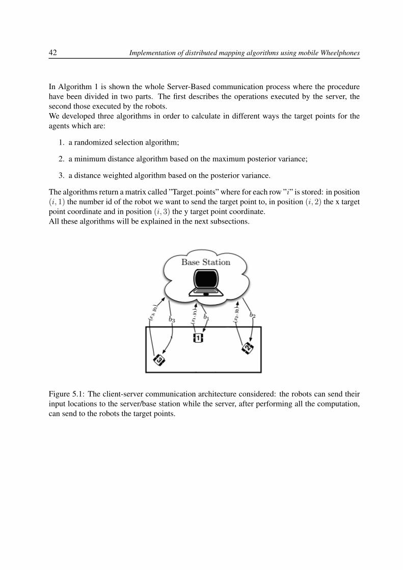
5.1 The client-server communication architecture considered: the robots can sendtheir input locations to the server/base station while the server, after performingall the computation, can send to the robots the target points. . . . . . . . . . . . . 42
5.2 Representation of µ(x) on the domainX and an example of estimation µ(x) afterk = 100 iteration using the Distance Weighted Algorithm. . . . . . . . . . . . . 47
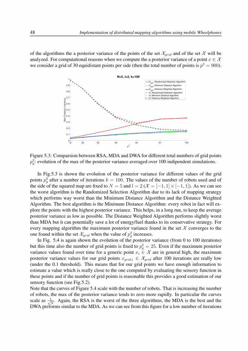
5.3 Comparsion between RSA, MDA and DWA for different total numbers of gridpoints p2g: evolution of the max of the posterior variance averaged over 100 in-dipendent simulations. . . . . . . . . . . . . . . . . . . . . . . . . . . . . . . . 48
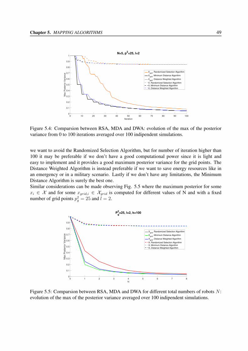
5.4 Comparsion between RSA, MDA and DWA: evolution of the max of the poste-rior variance from 0 to 100 iterations averaged over 100 indipendent simulations. 49
5.5 Comparsion between RSA, MDA and DWA for different total numbers of robotsN : evolution of the max of the posterior variance averaged over 100 indipendentsimulations. . . . . . . . . . . . . . . . . . . . . . . . . . . . . . . . . . . . . . 49
7
8 Implementation of distributed mapping algorithms using mobile Wheelphones
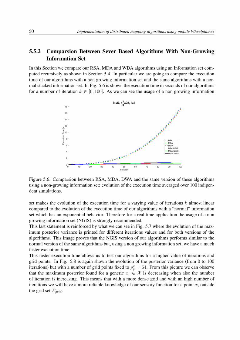
5.6 Comparsion between RSA, MDA, DWA and the same version of these algo-rithms using a non-growing information set: evolution of the execution timeaveraged over 100 indipendent simulations. . . . . . . . . . . . . . . . . . . . . 50
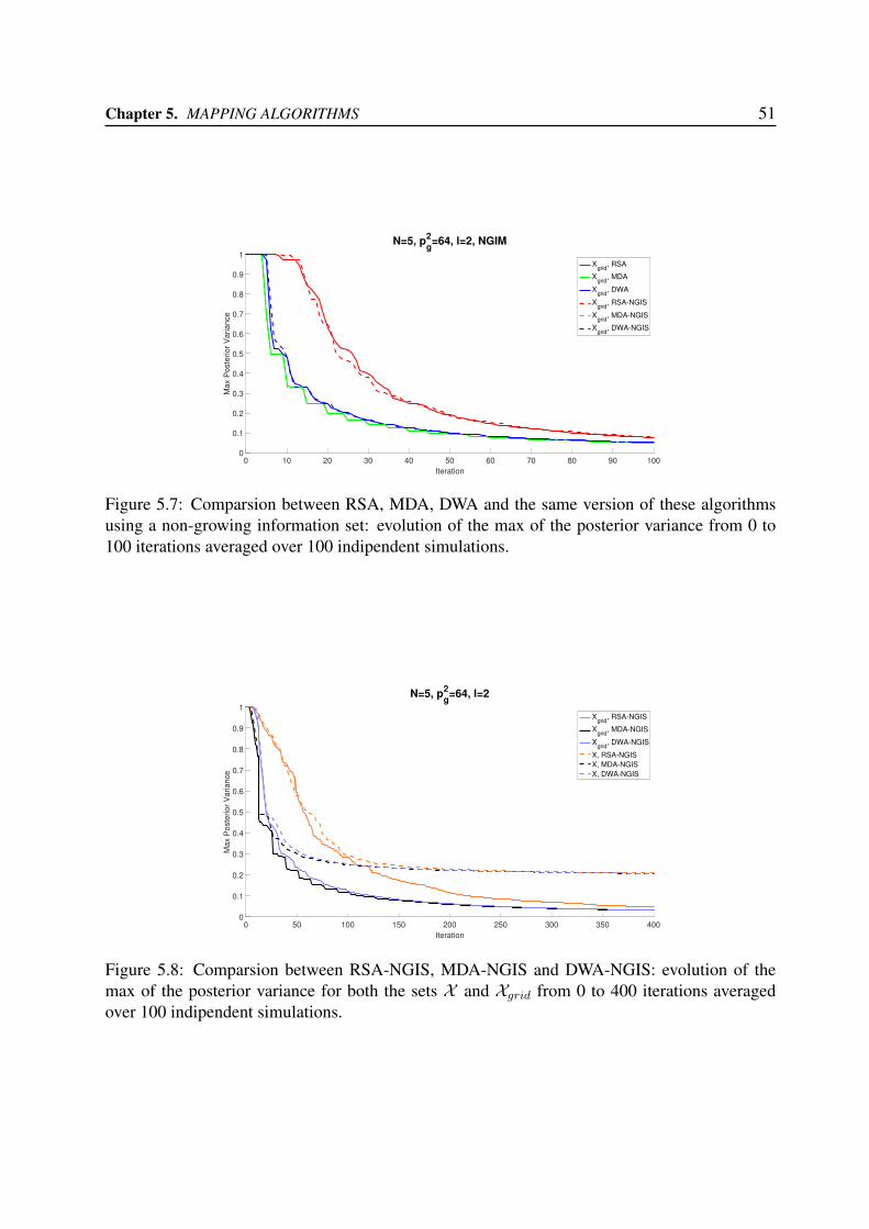
5.7 Comparsion between RSA, MDA, DWA and the same version of these algo-rithms using a non-growing information set: evolution of the max of the posteriorvariance from 0 to 100 iterations averaged over 100 indipendent simulations. . . 51
5.8 Comparsion between RSA-NGIS, MDA-NGIS and DWA-NGIS: evolution of themax of the posterior variance for both the sets X and Xgrid from 0 to 400 itera-tions averaged over 100 indipendent simulations. . . . . . . . . . . . . . . . . . 51
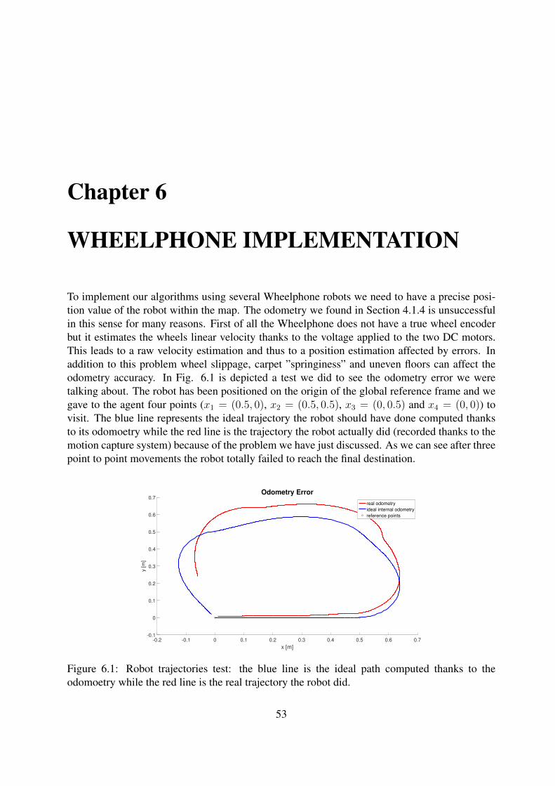
6.1 Robot trajectories test: the blue line is the ideal path computed thanks to theodomoetry while the red line is the real trajectory the robot did. . . . . . . . . . . 53
6.2 MAGIC Lab cameras configuration. . . . . . . . . . . . . . . . . . . . . . . . . 546.3 Triangulation . . . . . . . . . . . . . . . . . . . . . . . . . . . . . . . . . . . . 556.4 Two different cross patterns made of 4 markers . . . . . . . . . . . . . . . . . . 566.5 Wheelphone robots equipped with their own different cross markers pattern . . . 566.6 Reference Model . . . . . . . . . . . . . . . . . . . . . . . . . . . . . . . . . . 576.7 Example of a cross pattern of four markers. . . . . . . . . . . . . . . . . . . . . 586.8 Simulink Motion Capture Block scheme . . . . . . . . . . . . . . . . . . . . . . 616.9 Simulink Wheelphone Control Block scheme . . . . . . . . . . . . . . . . . . . 626.10 Detailed Simulink Wheelphone Point to Point Control Block scheme . . . . . . . 636.11 Robot trajectories comparison: internal odometry against motion capture control. 636.12 Position of the grid points within the map. . . . . . . . . . . . . . . . . . . . . . 646.13 Randomized Selection Algorithm trajectories. . . . . . . . . . . . . . . . . . . . 656.14 Minimum Distance Algorithm trajectories. . . . . . . . . . . . . . . . . . . . . . 666.15 Distance Weighted Algorithm trajectories. . . . . . . . . . . . . . . . . . . . . . 67
A.1 This diagram shows how the Target Language Compiler fits in with the codegeneration process. . . . . . . . . . . . . . . . . . . . . . . . . . . . . . . . . . 74
List of Tables
2.1 Receiving packet (sent by the mobile platform to the phone) description. . . . . . 192.2 flagRobotToPhone byte description. . . . . . . . . . . . . . . . . . . . . . . . . 202.3 Sending packet (sent by the phone to the mobile platform) description. . . . . . . 202.4 flagPhoneToRobot byte description. . . . . . . . . . . . . . . . . . . . . . . . . 21
9

Abstract
In this thesis we consider the problem of multi-robot mapping of an unknown event of interestin an indoor planar region where the communication between the agents is provided by a Wi-Fi network. Various exploration algorithms, most of which based on a nonparametric Gaussianregression approach to estimate an unknown sensory field, will be described and tested in bothcomputer simulation and real-world scenario using various Wheelphone robot devices. A sig-nificant attention will also be given to the driver building process which has been done in orderto establish a working interface between the Wheelphone device and the MATLAB / Simulinkenvironment.
11

Chapter 1
INTRODUCTION
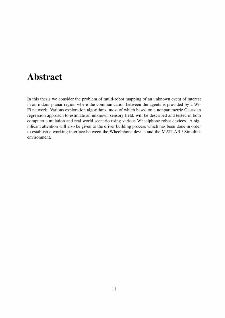
SLAM (Simultaneous Localization And Mapping) is the procedure that allows robots to success-fully map the environment and, at the same time, localize themselves on that map. This problemhas been well studied in the last thirty years because of the impact robotics has in many differentfields such as: civil, industrial and military. The concepts of mapping and localization in therobotic framework most of the times appear together because they are strictly connected, in fact,the knowledge of the position of a robot is of primary necessity to build a map, but at the sametime the knowledge of the map is useful to improve the localization estimation. In the eightiesand nineties the SLAM problem development was quite limited from technological constraintshowever nowadays, thanks to the appearance of cheap devices capable of good computation, thetrend is shifted to the extension of the SLAM problem into a multi-agent framework.What we want to do in this thesis is to map an unknown sensory function distributed in a planararea using a swarm of mobile robots in order to maximize the likelihood of detecting a specificevent. Once the exploration has been done a partitioning and coverage action can be started.
Figure 1.1: Example of a robotics swarm.
13
14 Implementation of distributed mapping algorithms using mobile Wheelphones
This task may have some interesting real applications. Imagine to have robots which can uselight for recharging their batteries. After they have explored the environment mapping the lightdistribution with their sensors they can eventually take position in the optimal place to accom-plish recharge. Another example could be the usage of wheeled devices to prevent and detect ablaze. In fact the probability of a fire is proportional to the temperature in a certain location andthe agents should cover more the areas where the temperature is higher.Three mapping algorithms based on a nonparametric estimation in the Gaussian regression frame-work will be presented and simulated along with a demo with true agents.The model of the robots used is called ”Wheelphone” and natively it can be programmed utiliz-ing the android language. Even though android and java are widely used, in our case (where wewant to test the control of the agent via rapid prototyping in an academic context) we prefer tobe able to use MATLAB and Simulink because they are flexible tools well known and used inour department.This led to the development of some driver interface files which description will be explained.
1.1 Mapping Literature ReviewIn modern robotics, the mapping task is the creation of a model of a real environment by robotsusing sensors to acquire topological information from the environment around them. The sensingtechnology commonly used today are: sonar, cameras, lasers and infrared. The sensors can beused singly or in a combination of them. Before of 2000, the majority of the relevant documentsabout exploration and mapping were focused on systems composed of a single robot [1, 2]; in thefollowing years, thanks to the better performance and to the low cost of sensors and embeddedcomputing architectures, and under the pressure of competitions and private companies (includ-ing military), the documentation about multi-robot systems able to communicate and exchangeinformation, has increased significantly [3].To solve the problem of map building and exploration over the years have been published dif-ferent approaches to the problem, each with pros and cons and more suited to certain operatingscenarios than others. Some of them are listed below.Yamauchi’s work is a milestones [4], which show a decentralised approach where each robotshares part of the information while keeping separate personal maps (also introducing the fun-damental concept of ”frontier”). With this approach each robot automatically decides the pointsof interest on the border where to go (frontier based exploration). However, this autonomousnavigation method lacks the coordination between robots, this implies the possibility that morerobots have the same objective, or that some of them explore areas already explored previouslyby others, this could cause a loss of efficiency.Simmons [5] has presented a centralised method in which robots merge the respective personalmaps in a common central map, from which a cost minimisation algorithm coordinates the move-ments of the explorers. Burgard [6] has shown that this coordinated approach has better perfor-mance of a non-coordinated one in the task resolution.Some multi-robot exploration approaches subdivide the surface to be explored thanks to a Voronoidiagram [7] in order to optimally divide the territory to be mapped between the various explor-
Chapter 1. INTRODUCTION 15
ers, this avoids that two robots explore the same surface area and thus this means that we canminimize the cost function time/energy.Another interesting field which an application is shown in [8] is the mapping and estimationfrom noisy measurements of a sensory field used to approximate the density function of an eventappearance. Most of the classically used techniques for identification are based on parametricestimation (maximum likelihood and prediction error methods) [9, 10] but they require persis-tent excitation to guarantee convergence of the parameter and the usage a fixed number of basisfunction requires the collection of at least the same number of samples to output a good estimate.These drawbacks make this methods slow. That’s why nonparametric estimation have been de-veloped: the main idea is to exploit black box models to estimate a function from examples-collected on input locations drawn from a fixed probability function [11, 12, 13]. Even if thisnonparametric approach in the worst case performs as good as the parametric one, its computa-tional complexity grows unbounded as the cube of collected samples. Efficient solutions basedon measurements truncation [14, 15] or Gaussian Markov [16] random fields have been pro-posed to overcome this problems. More recently the concept of stochastic gradient based onnoisy measurements of an unknown sensory function to perform an adaptive deployment of agroup of robots have been used [17]. In [18] a Kalman filtering procedure for non parametric es-timation is explained. The authors propose a two stage algorithm in which, based on informationon the posterior variance, the robot are spread throughout the space in order to achieve a goodestimate of the sensory function; once achieved a predefined threshold, the robots are forced tocover the monitored area.
1.2 ContributionsIn this work the main focus is to develop some mapping algorithms based on the estimationapproach used in [19] and to test them in a real world scenario with true robots.In particular we’ll give attention to:
1. the interface procedure between the robot and the MATLAB/Simulink software. That pointis fundamental because we’ll be able to design the control and to apply our algorithms inthe same flexible and well known environment. This will be precious in the case some oneelse in the future will expand our work;
2. the algorithms performance in terms of parameters in a real application.
1.3 OutlineThe remainder of the thesis is organized as follows:
• Chapter 2 presents the hardware and software tools we used to obtain our results.
• Chapter 3 describes the driver building procedure which has been done for making thecommunication between the Wheelphone device and the MATLAB / Simulink platformpossible.
16 Implementation of distributed mapping algorithms using mobile Wheelphones
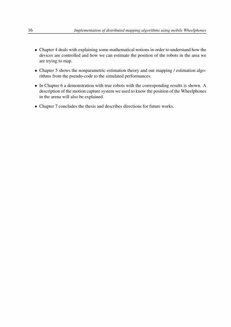
• Chapter 4 deals with explaining some mathematical notions in order to understand how thedevices are controlled and how we can estimate the position of the robots in the area weare trying to map.
• Chapter 5 shows the nonparametric estimation theory and our mapping / estimation algo-rithms from the pseudo-code to the simulated performances.
• In Chapter 6 a demonstration with true robots with the corresponding results is shown. Adescription of the motion capture system we used to know the position of the Wheelphonesin the arena will also be explained.
• Chapter 7 concludes the thesis and describes directions for future works.
Chapter 2
HARDWARE AND SOFTWARE SETUP
In this section we are going to illustrate and describe some of the main hardware and softwareresources which has been used in order to achieve our results. In the first place the algorithmshave been implemented and tested using a PC running MATLAB: the software can simulate theentire process from the robots movement to the mapping procedure. Afterwards the algorithmshave been tested with real two wheeled devices called ”Wheelphone”. The point to point controlis executed in real time on the smartphones which works as controller for the robots. The targetpoints for the agents are calculated from a base station thanks to the particular mapping algorithmchosen and then sent to the robots thanks to a Wi-Fi network. In fact all the mobile vehiclesand the main server are connected to the network and they can exchange information via UDPcommunication protocol. The agents knows their exact position in the environment thanks to amotion capture system.
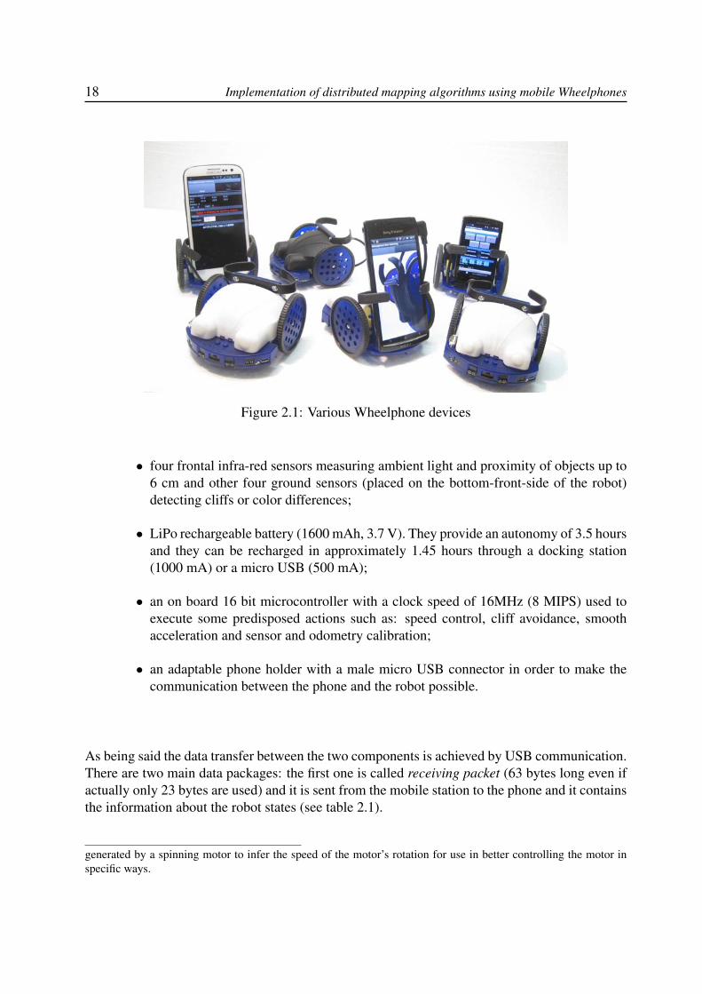
2.1 WheelphoneThe robot is shown if Fig. 2.1 and it’s composed of two main parts: an Android based smartphoneand a mobile platform.
1. The Android phone is used as a controller for the mobile platform. It communicateswith the mobile dock via USB. We can design the control with Simulink and thanks to theSimulink Coder and to the driver we implemented we are able to generate and run in realtime on the smartphone the C and C++ code generated from our model.The particular model chosen is the ”Samsung Galaxy S III mini” which comes with a smallsize factor, a 1 GHz dual core processor and 1 GB of RAM.
2. The two wheeled mobile dock is made up of a chassis (92 mm width, 102 mm length, 68mm height, with a weight of 200 g) containing:
• two DC motors, speed controlled with back EMF; 1
1In motor control and robotics, the term ”Back-EMF” often refers most specifically to actually using the voltage
17
18 Implementation of distributed mapping algorithms using mobile Wheelphones
Figure 2.1: Various Wheelphone devices
• four frontal infra-red sensors measuring ambient light and proximity of objects up to6 cm and other four ground sensors (placed on the bottom-front-side of the robot)detecting cliffs or color differences;
• LiPo rechargeable battery (1600 mAh, 3.7 V). They provide an autonomy of 3.5 hoursand they can be recharged in approximately 1.45 hours through a docking station(1000 mA) or a micro USB (500 mA);
• an on board 16 bit microcontroller with a clock speed of 16MHz (8 MIPS) used toexecute some predisposed actions such as: speed control, cliff avoidance, smoothacceleration and sensor and odometry calibration;
• an adaptable phone holder with a male micro USB connector in order to make thecommunication between the phone and the robot possible.
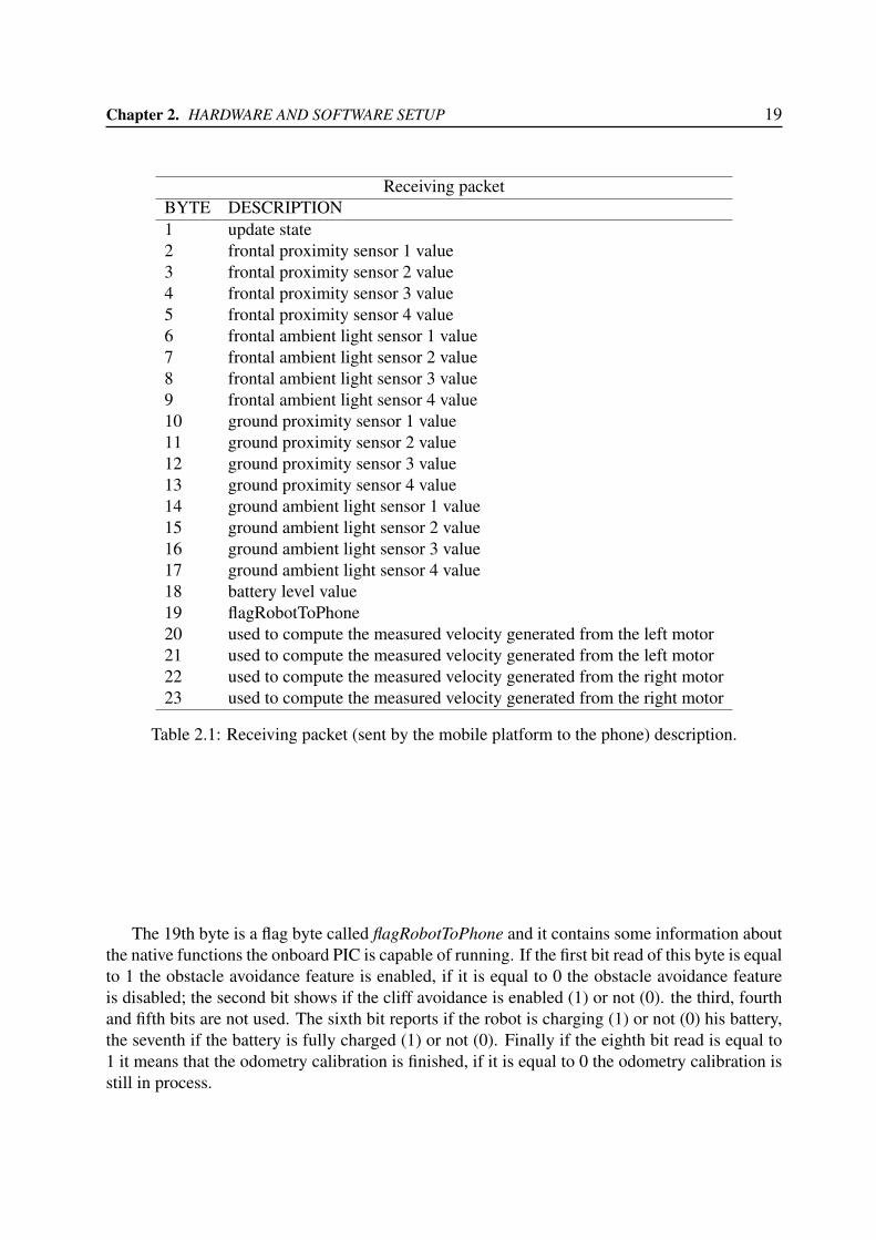
As being said the data transfer between the two components is achieved by USB communication.There are two main data packages: the first one is called receiving packet (63 bytes long even ifactually only 23 bytes are used) and it is sent from the mobile station to the phone and it containsthe information about the robot states (see table 2.1).
generated by a spinning motor to infer the speed of the motor’s rotation for use in better controlling the motor inspecific ways.
Chapter 2. HARDWARE AND SOFTWARE SETUP 19
Receiving packetBYTE DESCRIPTION1 update state2 frontal proximity sensor 1 value3 frontal proximity sensor 2 value4 frontal proximity sensor 3 value5 frontal proximity sensor 4 value6 frontal ambient light sensor 1 value7 frontal ambient light sensor 2 value8 frontal ambient light sensor 3 value9 frontal ambient light sensor 4 value10 ground proximity sensor 1 value11 ground proximity sensor 2 value12 ground proximity sensor 3 value13 ground proximity sensor 4 value14 ground ambient light sensor 1 value15 ground ambient light sensor 2 value16 ground ambient light sensor 3 value17 ground ambient light sensor 4 value18 battery level value19 flagRobotToPhone20 used to compute the measured velocity generated from the left motor21 used to compute the measured velocity generated from the left motor22 used to compute the measured velocity generated from the right motor23 used to compute the measured velocity generated from the right motor
Table 2.1: Receiving packet (sent by the mobile platform to the phone) description.
The 19th byte is a flag byte called flagRobotToPhone and it contains some information aboutthe native functions the onboard PIC is capable of running. If the first bit read of this byte is equalto 1 the obstacle avoidance feature is enabled, if it is equal to 0 the obstacle avoidance featureis disabled; the second bit shows if the cliff avoidance is enabled (1) or not (0). the third, fourthand fifth bits are not used. The sixth bit reports if the robot is charging (1) or not (0) his battery,the seventh if the battery is fully charged (1) or not (0). Finally if the eighth bit read is equal to1 it means that the odometry calibration is finished, if it is equal to 0 the odometry calibration isstill in process.
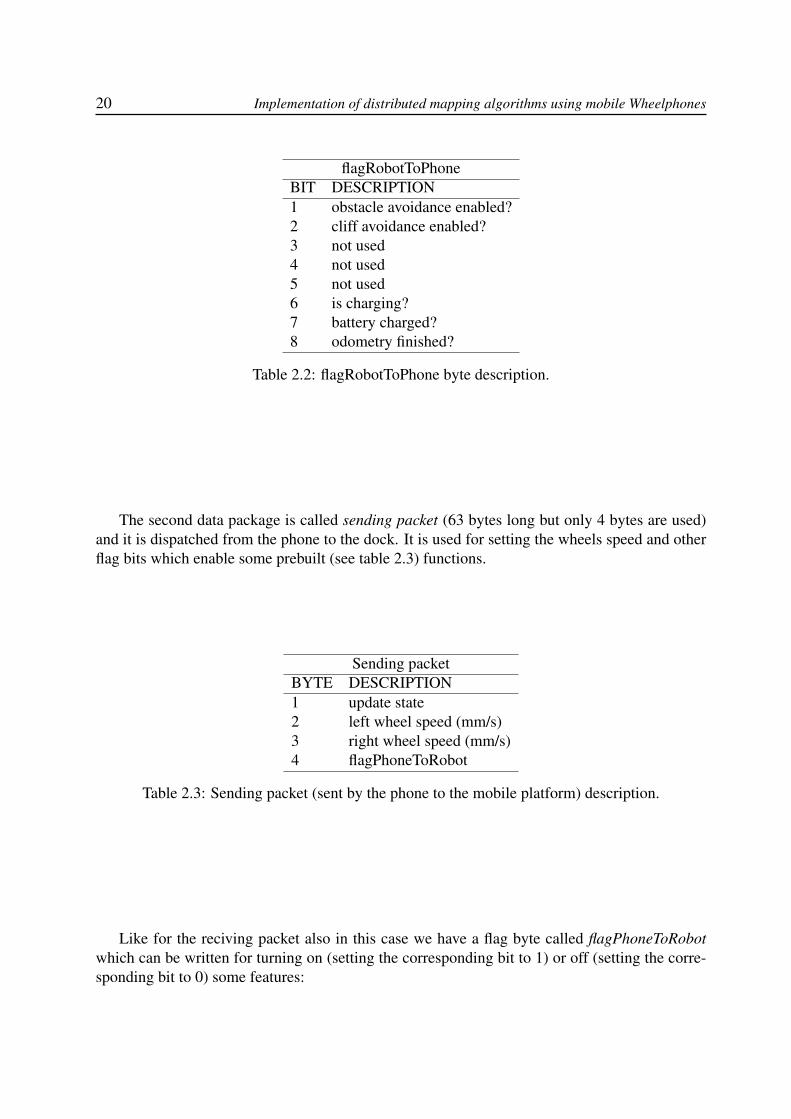
20 Implementation of distributed mapping algorithms using mobile Wheelphones
flagRobotToPhoneBIT DESCRIPTION1 obstacle avoidance enabled?2 cliff avoidance enabled?3 not used4 not used5 not used6 is charging?7 battery charged?8 odometry finished?
Table 2.2: flagRobotToPhone byte description.
The second data package is called sending packet (63 bytes long but only 4 bytes are used)and it is dispatched from the phone to the dock. It is used for setting the wheels speed and otherflag bits which enable some prebuilt (see table 2.3) functions.
Sending packetBYTE DESCRIPTION1 update state2 left wheel speed (mm/s)3 right wheel speed (mm/s)4 flagPhoneToRobot
Table 2.3: Sending packet (sent by the phone to the mobile platform) description.
Like for the reciving packet also in this case we have a flag byte called flagPhoneToRobotwhich can be written for turning on (setting the corresponding bit to 1) or off (setting the corre-sponding bit to 0) some features:

Chapter 2. HARDWARE AND SOFTWARE SETUP 21
flagPhoneToRobotBIT DESCRIPTION1 speed controller2 soft acceleration3 obstacle avoidance4 cliff avoidance5 calibrate sensors6 calibrate odometry7 not used8 not used
Table 2.4: flagPhoneToRobot byte description.
2.2 Motion Capture SystemA motion capture system is a device capable of tracking and recording the movements of anobject in a tridimensional space. The one located in our laboratory is an optical motion capturesystem (Fig. 2.2) which utilizes the data coming from two or more cameras to reconstruct theposition of the agent in the 3D space thanks to a triangulation algorithm. Triangulation accuracyis strongly related to the positions and orientations of the cameras. Thus, the configuration ofthe camera network has a critical impact on performance. The most common approach is basedon infrared marker recognition. The markers are small objects capable of reflecting the infrared
Figure 2.2: An optical motion capture system representation
light emitted from sources near the cameras. The cameras are equipped with an IR-pass filter and
22 Implementation of distributed mapping algorithms using mobile Wheelphones
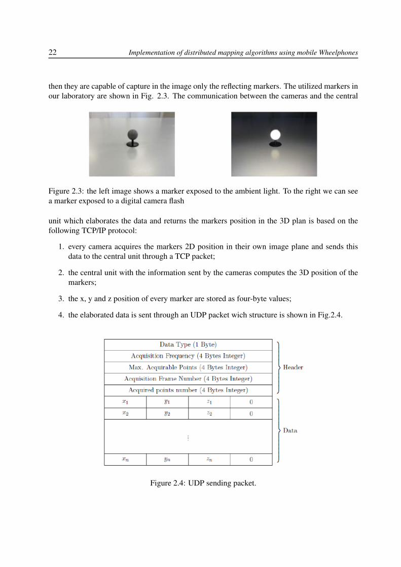
then they are capable of capture in the image only the reflecting markers. The utilized markers inour laboratory are shown in Fig. 2.3. The communication between the cameras and the central
Figure 2.3: the left image shows a marker exposed to the ambient light. To the right we can seea marker exposed to a digital camera flash
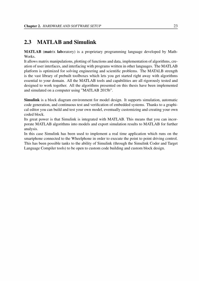
unit which elaborates the data and returns the markers position in the 3D plan is based on thefollowing TCP/IP protocol:
1. every camera acquires the markers 2D position in their own image plane and sends thisdata to the central unit through a TCP packet;
2. the central unit with the information sent by the cameras computes the 3D position of themarkers;
3. the x, y and z position of every marker are stored as four-byte values;
4. the elaborated data is sent through an UDP packet wich structure is shown in Fig.2.4.
Figure 2.4: UDP sending packet.
Chapter 2. HARDWARE AND SOFTWARE SETUP 23
2.3 MATLAB and SimulinkMATLAB (matrix laboratory) is a proprietary programming language developed by Math-Works.It allows matrix manipulations, plotting of functions and data, implementation of algorithms, cre-ation of user interfaces, and interfacing with programs written in other languages. The MATLABplatform is optimized for solving engineering and scientific problems. The MATALB strengthis the vast library of prebuilt toolboxes which lets you get started right away with algorithmsessential to your domain. All the MATLAB tools and capabilities are all rigorously tested anddesigned to work together. All the algorithms presented on this thesis have been implementedand simulated on a computer using ”MATLAB 2015b”.
Simulink is a block diagram environment for model design. It supports simulation, automaticcode generation, and continuous test and verification of embedded systems. Thanks to a graphi-cal editor you can build and test your own model, eventually customizing and creating your owncoded block.Its great power is that Simulink is integrated with MATLAB. This means that you can incor-porate MATLAB algorithms into models and export simulation results to MATLAB for furtheranalysis.In this case Simulink has been used to implement a real time application which runs on thesmartphone connected to the Wheelphone in order to execute the point to point driving control.This has been possible tanks to the ability of Simulink (through the Simulink Coder and TargetLanguage Compiler tools) to be open to custom code building and custom block design.

Chapter 3
DRIVER DEVELOPMENT PROCESS
Once that the MATLAB / Simulink platform was chosen to control the Wheelphone an effort hadto be made to interface the robot with the software. We want our control to be executed fromthe android phone attached to the mobile dock. This can be made thanks to Simulink and tothe Simulink Coder (formerly Real-Time Workshop) which generates and executes C and C++code from Simulink diagrams, Stateflow charts, and MATLAB functions. The generated sourcecode can be used for real-time and non-real-time applications, including simulation acceleration,rapid prototyping (this is our case: rapid prototyping provides a fast and inexpensive way forcontrol and signal processing engineers to verify designs early and evaluate design tradeoffs),and hardware-in-the-loop testing. In this way we can tune and monitor the generated code usingSimulink or run and interact with the code outside MATLAB and Simulink. Thus, after we cre-ate a Simulink block for the Wheelphone thanks to an S-function, we must instruct the SimulinkCoder on how to build code from this custom block. This can be achieved with the help of theTarget Language Compiler (TLC) which provides a great deal of freedom for altering, optimiz-ing, and enhancing the generated code. One of the most important TLC features is that it lets youinline S-functions that you wrote to add your own algorithms, device drivers, and custom blocksto a Simulink model.
3.1 S-function Design
An S-function is a computer lenguage description of a Simulink block written in MATLAB, C,C++ or Fortran.We decided to write the Wheelphone S-function, called ”sfun wheelphone.c”, in C code. C writ-ten S-functions are complied as MEX files using the command: mex sfun wheelphone.c.S-functions use a special calling syntax called ”the S-function API” that enables you to interactwith the Simulink engine. To understand how the S-function we wrote works we first need toknow how the Simulink engine simulates a model.
25
26 Implementation of distributed mapping algorithms using mobile Wheelphones
3.1.1 Simulation Stages
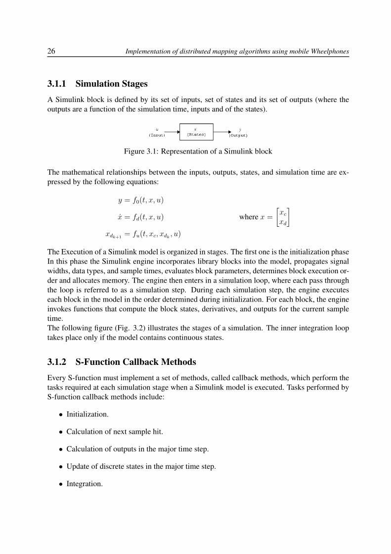
A Simulink block is defined by its set of inputs, set of states and its set of outputs (where theoutputs are a function of the simulation time, inputs and of the states).
Figure 3.1: Representation of a Simulink block
The mathematical relationships between the inputs, outputs, states, and simulation time are ex-pressed by the following equations:
y = f0(t, x, u)
x = fd(t, x, u) where x =
[xcxd
]xdk+1
= fu(t, xc, xdk , u)
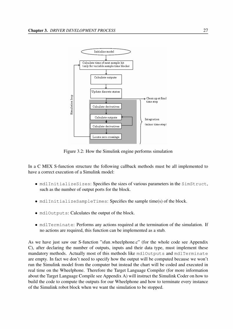
The Execution of a Simulink model is organized in stages. The first one is the initialization phaseIn this phase the Simulink engine incorporates library blocks into the model, propagates signalwidths, data types, and sample times, evaluates block parameters, determines block execution or-der and allocates memory. The engine then enters in a simulation loop, where each pass throughthe loop is referred to as a simulation step. During each simulation step, the engine executeseach block in the model in the order determined during initialization. For each block, the engineinvokes functions that compute the block states, derivatives, and outputs for the current sampletime.The following figure (Fig. 3.2) illustrates the stages of a simulation. The inner integration looptakes place only if the model contains continuous states.
3.1.2 S-Function Callback Methods
Every S-function must implement a set of methods, called callback methods, which perform thetasks required at each simulation stage when a Simulink model is executed. Tasks performed byS-function callback methods include:
• Initialization.
• Calculation of next sample hit.
• Calculation of outputs in the major time step.
• Update of discrete states in the major time step.
• Integration.
Chapter 3. DRIVER DEVELOPMENT PROCESS 27
Figure 3.2: How the Simulink engine performs simulation
In a C MEX S-function structure the following callback methods must be all implemented tohave a correct execution of a Simulink model:
• mdlInitializeSizes: Specifies the sizes of various parameters in the SimStruct,such as the number of output ports for the block.
• mdlInitializeSampleTimes: Specifies the sample time(s) of the block.
• mdlOutputs: Calculates the output of the block.
• mdlTerminate: Performs any actions required at the termination of the simulation. Ifno actions are required, this function can be implemented as a stub.
As we have just saw our S-function ”sfun wheelphone.c” (for the whole code see AppendixC), after declaring the number of outputs, inputs and their data type, must implement thesemandatory methods. Actually most of this methods like mdlOutputs and mdlTerminateare empty. In fact we don’t need to specify how the output will be computed because we won’trun the Simulink model from the computer but instead the chart will be coded and executed inreal time on the Wheelphone. Therefore the Target Language Compiler (for more informationabout the Target Language Compile see Appendix A) will instruct the Simulink Coder on how tobuild the code to compute the outputs for our Wheelphone and how to terminate every instanceof the Simulink robot block when we want the simulation to be stopped.
28 Implementation of distributed mapping algorithms using mobile Wheelphones
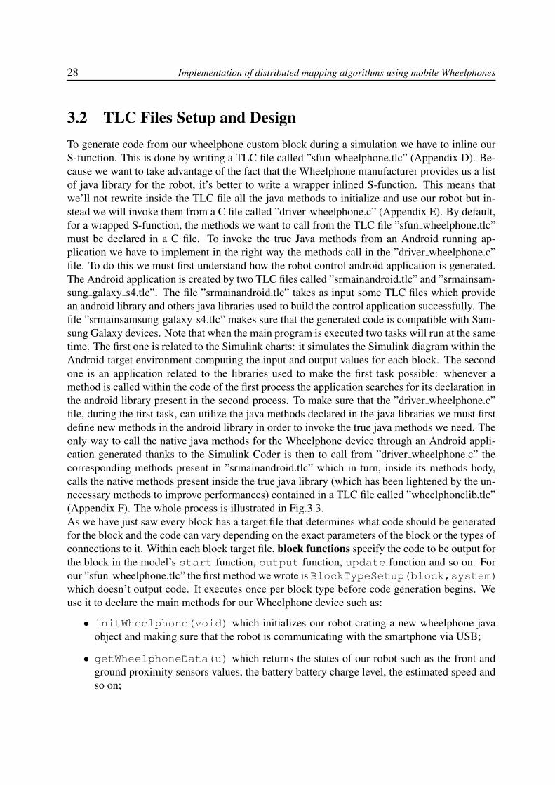
3.2 TLC Files Setup and DesignTo generate code from our wheelphone custom block during a simulation we have to inline ourS-function. This is done by writing a TLC file called ”sfun wheelphone.tlc” (Appendix D). Be-cause we want to take advantage of the fact that the Wheelphone manufacturer provides us a listof java library for the robot, it’s better to write a wrapper inlined S-function. This means thatwe’ll not rewrite inside the TLC file all the java methods to initialize and use our robot but in-stead we will invoke them from a C file called ”driver wheelphone.c” (Appendix E). By default,for a wrapped S-function, the methods we want to call from the TLC file ”sfun wheelphone.tlc”must be declared in a C file. To invoke the true Java methods from an Android running ap-plication we have to implement in the right way the methods call in the ”driver wheelphone.c”file. To do this we must first understand how the robot control android application is generated.The Android application is created by two TLC files called ”srmainandroid.tlc” and ”srmainsam-sung galaxy s4.tlc”. The file ”srmainandroid.tlc” takes as input some TLC files which providean android library and others java libraries used to build the control application successfully. Thefile ”srmainsamsung galaxy s4.tlc” makes sure that the generated code is compatible with Sam-sung Galaxy devices. Note that when the main program is executed two tasks will run at the sametime. The first one is related to the Simulink charts: it simulates the Simulink diagram within theAndroid target environment computing the input and output values for each block. The secondone is an application related to the libraries used to make the first task possible: whenever amethod is called within the code of the first process the application searches for its declaration inthe android library present in the second process. To make sure that the ”driver wheelphone.c”file, during the first task, can utilize the java methods declared in the java libraries we must firstdefine new methods in the android library in order to invoke the true java methods we need. Theonly way to call the native java methods for the Wheelphone device through an Android appli-cation generated thanks to the Simulink Coder is then to call from ”driver wheelphone.c” thecorresponding methods present in ”srmainandroid.tlc” which in turn, inside its methods body,calls the native methods present inside the true java library (which has been lightened by the un-necessary methods to improve performances) contained in a TLC file called ”wheelphonelib.tlc”(Appendix F). The whole process is illustrated in Fig.3.3.As we have just saw every block has a target file that determines what code should be generatedfor the block and the code can vary depending on the exact parameters of the block or the types ofconnections to it. Within each block target file, block functions specify the code to be output forthe block in the model’s start function, output function, update function and so on. Forour ”sfun wheelphone.tlc” the first method we wrote is BlockTypeSetup(block,system)which doesn’t output code. It executes once per block type before code generation begins. Weuse it to declare the main methods for our Wheelphone device such as:
• initWheelphone(void) which initializes our robot crating a new wheelphone javaobject and making sure that the robot is communicating with the smartphone via USB;
• getWheelphoneData(u) which returns the states of our robot such as the front andground proximity sensors values, the battery battery charge level, the estimated speed andso on;
Chapter 3. DRIVER DEVELOPMENT PROCESS 29
Figure 3.3: The wrapped inlined S-function sfun wheelphone.tlc calls methods from the C filesfun wheelphone.c wich in turn calls methods from the native Wheelphone java library. Thislibrary is accessible in real time during the execution of the android app thanks to a TLC filecalled wheelphonelib.tlc
30 Implementation of distributed mapping algorithms using mobile Wheelphones
• setWheelphoneSpeed(l,r) which set the left and right wheel speed in mm/s.
The second function is Start(block, system). The code inside the Start function exe-cutes once and only once. We included a Start function to initialize the Wheelphone (calling themethod initWheelphone) at the beginning of the simulation.Every block should then include an Outputs(block, system) function which of coursespecifies how to compute the outputs for our S-function. In this case, after defining the input andoutput variables, we just invoke the methods getWheelphoneData andsetWheelphoneSpeed.
Chapter 4
MATHEMATICAL PRELIMINARIES
4.1 Mobile Robot KinematicsMobile Robot Kinematics is the dynamic model of how a mobile robot behaves. In mobilerobotics, we need to understand the mechanical behavior of the robot both in order to design andto control a mobile agent hardware. More specifically the Mobile Robot Kinematics is a usefultool when it comes to position and motion estimation. The process of understanding the motionsof a robot begins with the process of describing the contribution each wheel provides for motion.Each wheel provides motion but also imposes some constraints such as refusing to skid laterally.
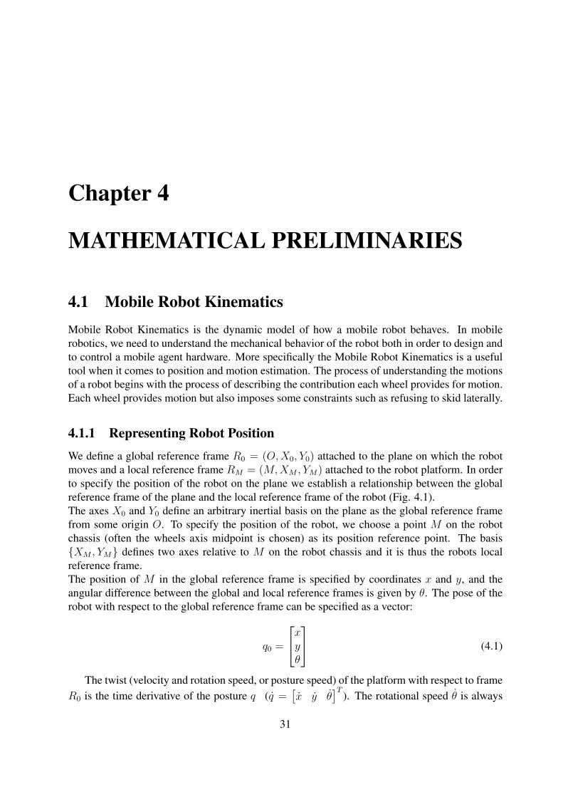
4.1.1 Representing Robot PositionWe define a global reference frame R0 = (O,X0, Y0) attached to the plane on which the robotmoves and a local reference frame RM = (M,XM , YM) attached to the robot platform. In orderto specify the position of the robot on the plane we establish a relationship between the globalreference frame of the plane and the local reference frame of the robot (Fig. 4.1).The axes X0 and Y0 define an arbitrary inertial basis on the plane as the global reference framefrom some origin O. To specify the position of the robot, we choose a point M on the robotchassis (often the wheels axis midpoint is chosen) as its position reference point. The basis{XM , YM} defines two axes relative to M on the robot chassis and it is thus the robots localreference frame.The position of M in the global reference frame is specified by coordinates x and y, and theangular difference between the global and local reference frames is given by θ. The pose of therobot with respect to the global reference frame can be specified as a vector:
q0 =
xyθ
(4.1)
The twist (velocity and rotation speed, or posture speed) of the platform with respect to frameR0 is the time derivative of the posture q (q =
[x y θ
]T). The rotational speed θ is always
31
32 Implementation of distributed mapping algorithms using mobile Wheelphones
around the z axis common to all frames, so it does not depend on the frame chosen to express itbut the components of the velocity of point M do vary depending on the frame. We will need toexpress the twist of the robot either in R0 or in RM . The orthogonal rotation matrix R(θ) is usedto map motion in the robot local reference frame {XM , YM} to motion in the global referenceframe {X0, Y0}:
R(θ) =
cos θ − sin θ 0sin θ cos θ 0
0 0 1
(4.2)
q0 = R(θ)qM (4.3)
Of course we also have that:
R(θ)−1 =
cos θ sin θ 0− sin θ cos θ 0
0 0 1
(4.4)
qM = R(θ)−1q0 (4.5)
Figure 4.1: The global reference frame and the robot local reference frame
4.1.2 Kinematic ConstraintsThe motion of a differential-drive mobile robot is limited by two non-holonomic constraint equa-tions, which are obtained by two main assumptions:
• No lateral slip motion: in the robot frame this condition means that the velocity of thecenter-point M is zero along the lateral axis: yM = 0. Thus, remembering thatqM = R(θ)−1q0, this translates in the global reference frame as:
yM =[− sin θ cos θ 0
] xyθ
= 0 =⇒ −x sin θ + y cos θ = 0
Chapter 4. MATHEMATICAL PRELIMINARIES 33
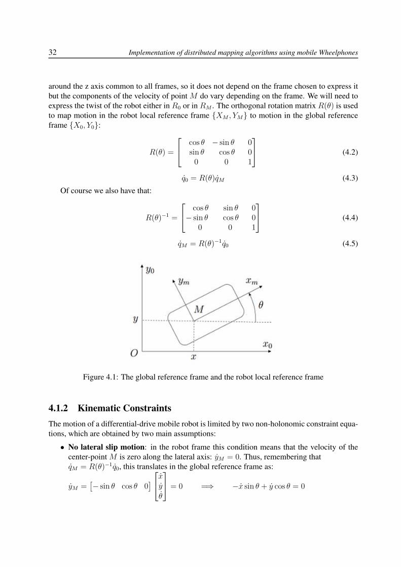
• Pure rolling constraint: each wheel maintains a single contact point P with the ground(Fig. 4.2). There is no slipping of the wheel in its longitudinal axis and no skidding in its
orthogonal axis so we can write:
{vr = Rϕr
vl = Rϕl
Figure 4.2: Pure Rolling Motion Constraint.
4.1.3 Kinematic Model for Differential Drive RobotMany mobile robots use a drive mechanism known as differential drive. It consists of two drivewheels (each with radius R) mounted on a common axis; each wheel can independently beingdriven either forward or backward.The Forward Kinematics provides an estimate of the robots position given its geometry and thespeeds of its wheels.Given a point M positioned in the midpoint of the wheels axis, each wheel is at distance L fromM . Given R, L, and the spinning speed of each wheel, ϕr and ϕl , a forward kinematic modelcan predict the robots overall speed in the global reference frame:
q0 =
xyθ
= f(L,R, θ, ϕr, ϕl) (4.6)
Suppose (as shown in Fig. 4.3) that the robots local reference frame is aligned such that therobot moves forward along +XM . First consider the contribution of each wheels spinning speedto the translation speed at M in the direction of +XM . To find the linear velocity in the directionof +XM each wheel contributes one half of the total speed (if only one wheel is spinning M ishalfway between the two wheels and it will move instantaneously with half the speed):xMr = 1
2Rϕr and xMl = 1
2Rϕl.
Consider now a differential robot in which each wheel spins with equal speed but in oppositedirections. The angular velocity about θ is again calculated from the contribution of the two
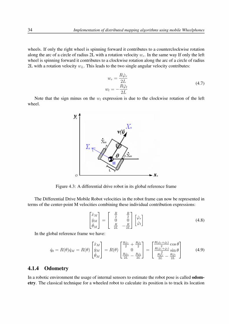
34 Implementation of distributed mapping algorithms using mobile Wheelphones
wheels. If only the right wheel is spinning forward it contributes to a counterclockwise rotationalong the arc of a circle of radius 2L with a rotation velocity wr. In the same way If only the leftwheel is spinning forward it contributes to a clockwise rotation along the arc of a circle of radius2L with a rotation velocity wL. This leads to the two single angular velocity contributes:
wr =Rϕr2L
wl = −Rϕl2L
(4.7)
Note that the sign minus on the wl expression is due to the clockwise rotation of the leftwheel.
Figure 4.3: A differential drive robot in its global reference frame
The Differential Drive Mobile Robot velocities in the robot frame can now be represented interms of the center-point M velocities combining these individual contribution expressions:xMyM
θM
=
R2
R2
0 0R2L− R
2L
[ϕrϕl
](4.8)
In the global reference frame we have:
q0 = R(θ)qM = R(θ)
xMyMθM
= R(θ)
Rϕr2 + Rϕl2
0Rϕr2L− Rϕl
2L
=
R(ϕr+ϕl)2
cos θR(ϕr+ϕl)
2sin θ
Rϕr2L− Rϕl
2L
(4.9)
4.1.4 OdometryIn a robotic environment the usage of internal sensors to estimate the robot pose is called odom-etry. The classical technique for a wheeled robot to calculate its position is to track its location
Chapter 4. MATHEMATICAL PRELIMINARIES 35
through a series of measurements of the rotations of the robots wheels. Odometry requires amethod for accurately counting the rotation of the robot and, with this information, estimate theleft and right wheel velocities. Therefore relative position estimation is extremely dependent onthe measurement of the robots velocity. Once we have our left and right spinning velocities wecan compute the equation 4.9 and obtain our pose integrating x y and θ:
x =1
2
∫ t
0
[vr(t) + vl(t)] cos(θ(t)) dx
y =1
2
∫ t
0
[vr(t) + vl(t)] sin(θ(t)) dx
θ =1
2L
∫ t
0
[vr(t)− vl(t)] dx
(4.10)
4.2 Point to Point ControlThe algorithms we will see in Chapter 5 return some points in the plane the robots must reach totake a noisy measurement of the sensory function we want to map. To make these movementspossible a driving control method must be designed.Therefore consider the problem of moving toward a goal point (xr, yr) in the plane. We willcontrol the robots velocity to be proportional to its distance from the goal:
v = Kv · ed (4.11)
where ed is the distance:ed =
√(xr − x)2 + (yr − y)2
Let’s recall that the x and y coordinate of the robot are represented by the position in space ofthe wheels axis midpoint M .To steer toward the goal we must compute the angle between the x axis of the global referenceframe and the straight line passing through the goal point and the origin of the robot referenceframe. This vehicle-relative angle is:
θr = tan−1(yr − yxr − x
)
To make the robot face the right direction we impose an angular velocity proportional to theangular error eθ = θr − θ:
w = Kw · eθ (4.12)
Note that x, y and θ are estimated thanks to the formulas (4.10) from the robot actual velocity.Since the Wheelphone takes as input the left and right velocities we want to convert this angularvelocity into linear velocities. We also want that the robot may be able to turn itself around hiswheels axis midpoint M ; that’s why we choose the left and right linear velocities as vl = −vr:
vl = −w · Lvr = w · L
(4.13)
36 Implementation of distributed mapping algorithms using mobile Wheelphones
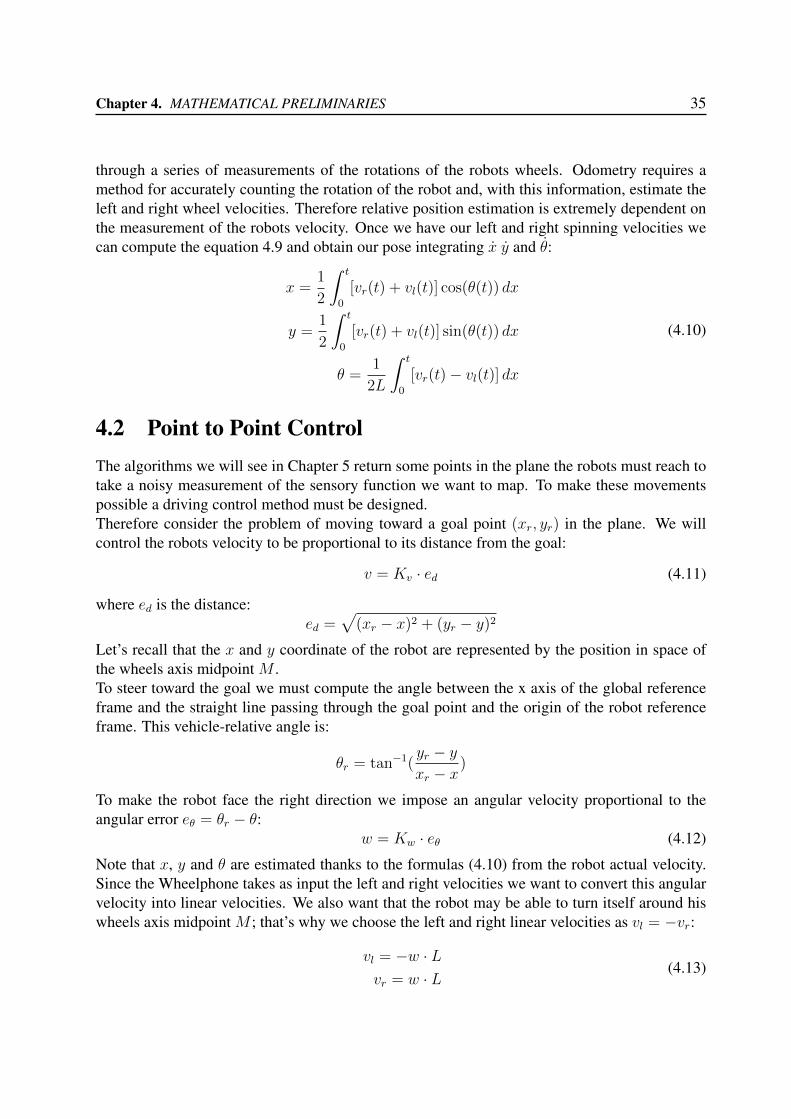
Finally, to make the robot moves faster toward the goal point, we sum for each wheel the ve-locity component calculated from the distance ed (4.11) and the one calculated from the angularvelocity (4.13):
vl = Kv · ed −Kw · eθ · Lvr = Kv · ed +Kw · eθ · L
(4.14)
This control procedure is schematized in Fig.4.4.
Figure 4.4: Point to point control chart
4.2.1 Point to Point Control Simulink Model With Odometry
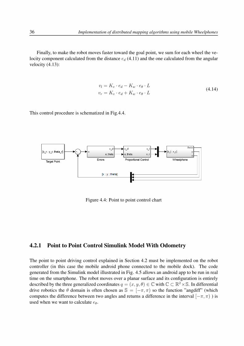
The point to point driving control explained in Section 4.2 must be implemented on the robotcontroller (in this case the mobile android phone connected to the mobile dock). The codegenerated from the Simulink model illustrated in Fig. 4.5 allows an android app to be run in realtime on the smartphone. The robot moves over a planar surface and its configuration is entirelydescribed by the three generalized coordinates q = (x, y, θ) ∈ C with C ⊂ R2×S. In differentialdrive robotics the θ domain is often chosen as S = [−π, π) so the function ”angdiff” (whichcomputes the difference between two angles and returns a difference in the interval [−π, π) ) isused when we want to calculate eθ.
Chapter 4. MATHEMATICAL PRELIMINARIES 37
Figure 4.5: Simulink model of the point to point control
Due to the fact that the wheels of the Wheelphone robot are not equipped with true encodersthe actual velocity estimation of the device is not accurate. If we consider also the fact we needto integrate this velocity in order to gain access to the robot pose (4.14) the result is that theestimated position of the wheelphone over time becomes unreliable and the control becomesalso inefficient. To have a good pose estimation during the real implementation of the mappingalgorithms we will use a motion capture system.

Chapter 5
MAPPING ALGORITHMS
In this section we present three algorithms based on nonparametric estimation.
5.1 Nonparametric Estimation
Let f : A −→ R denote an unknown deterministic function defined on the compact setA ⊂ Rn. Assume to have a set of S ∈ N noisy measurements taken on the input locations ai, i.e.{ai, yi}Si=1, of the form:
yi = f(ai) + vi, i = 1, . . . . . , S (5.1)
where vi is a zero-mean Gaussian noise with variance σ2, i.e. vi ∼ N (0, σ2) , independent of theunknown function. Given the data set {ai, yi}Si=1, one of the most used approaches to estimate frelies upon the Tikhonov regularization theory (see Appendix B) [20].Let’s suppose that f is a zero-mean Gaussian field with covariance, also called kernel K:
K : A×A −→ R.
Defining the set containing all the yi measurements taken at the ai input location as the informa-tion set I:
I = {(ai, yi) | i ∈ {1, . . . . . , S}}
and exploiting known results on estimation of Gaussian random fields, one obtains that the min-imum variance estimate of f given I is a linear combination of the kernel sections K(ai, ·):
f(x) = E[f(a)|I] =S∑i=1
ciK(ai, a), x ∈ A (5.2)
where the expansion coefficients ci are obtained as:
39
40 Implementation of distributed mapping algorithms using mobile Wheelphones
c1c2...cS
= (K + σ2I)−1
y1y2...yS
(5.3)
while the matrix K is obtained by evaluating the kernel at the input-locations, i.e.
K =
K(a1, a1) · · · K(a1, aS)... . . . ...
K(aS, a1) · · · K(aS, aS)
. (5.4)
Moreover, the a posteriori variance of the estimate, in a generic location of the plane a ∈ A is:
V (a) = V ar[f(a)|I] =
= K(a, a)−[K(a1, a) · · · K(aS, a)
](K + σ2I)−1
K(a1, a)...
K(aS, a)
(5.5)
The main problem with this approach is that we need to store more and more input-locationsand noisy measurements as time increases to compute the estimate. Indeed, the most expensiveoperation is the inversion of the S × S matrix (K + σ2I) which requires O(S3) operations. Thiswill eventually lead to a memory and computational consuming process which grows unboundedwith S.
5.2 Problem DescriptionWe consider a swarm of N robots allowed to move in a planar region represented by the convexset X . The goal is to design algorithms to map and estimate an unknown sensory functionµ : X −→ R. We assume to take µ as a realization of a Gaussian random field with covarianceK : X × X −→ R.We will consider the Gaussian kernel:
K(x, x′) = λe− ‖x−x
′‖2
2ξ2 , λ = 1, ξ = 0.2. (5.6)
We also assume, for a computer simulation purpose, that every agent i ∈ {1, . . . , N} can:
• take noisy measurements of µ in the form:
y(xi) = µ(xi) + vi, (5.7)
where vi ∼ N (0, σ2) is independent from µ and from all the noise measurements vj;
Chapter 5. MAPPING ALGORITHMS 41
• communicate with a server/base station or to closely located agents;
• move to a certain target-point bi respecting the following update law:xi,k+1 = xi,k + ui,k, ∀i ∈ {1, . . . , N},which says that every robot can move from location xi,k at time t = kT to any desiredlocation xi,k+1 = bi at time t = (k + 1)T .
To make simulations faster and suitable for for a numerical implementation we decided to dis-cretize the working area X . The idea is to constrain the robots to collect measurements onlyfrom a set of predetermined finite number of input locations which are obtained thanks to aspatial discretization of the continuous convex domain X :
Definition 5.1. Consider the finite set of m input locations Xgrid = {xgrid,1, . . . , xgrid,m} ⊂ Xwhere X ⊂ R2 is a convex closed polygon. Given the scalar ∆ > 0, we say that the set Xgridforms a sampled space of resolution ∆ if:
mini=1,...,m
‖xgrid,i − x‖ ≤ ∆ ∀x ∈ X (5.8)
5.3 Server-Based AlgorithmsThe following algorithms are based on a client-server communication architecture where therobots are allowed to communicate with a central server which can:
• store all the measurements taken by the robots;
• store the last position of the agents within the the convex setX in a matrix called ”Robot positions”where in each row ”i” is stored: in position (i, 1) the robot id number, in position (i, 2) thex robot coordinate and in position (i, 3) the y robot coordinate;
• compute the target points to visit and send information to the robots every T seconds;
• compute and store an estimate µ of the function µ and its posterior variance V .
We also suppose that every robot i ∈ {1, . . . , N} can take only one measurement in the from(5.7) within the time window t ∈ (kT, (K + 1)T ), k ∈ N. Once the measurement has beencollected it is immediately transmitted to the server which stores it in memory. Then the servercomputes,depending on the algorithm used, the next target locations for each robot. By definingwith Jk the set of measurements received by the server at iteration k, i.e.
Jk := {(xi,k, yi,k)|i = 1, . . . , N}, xi,k ∈ Xgrid ⊂ X
the total information set Ik available at server at iteration k can be computed as:
Ik = Ik−1 ∪ Jk, ∀k ≥ 1, I0 6= ∅.
Thanks to the information set Ik the server can store in his memory the estimate µk(x) of thefunction µ(x) and its posterior variance Vk(x) computed according to equations (5.2) and (5.5).
42 Implementation of distributed mapping algorithms using mobile Wheelphones
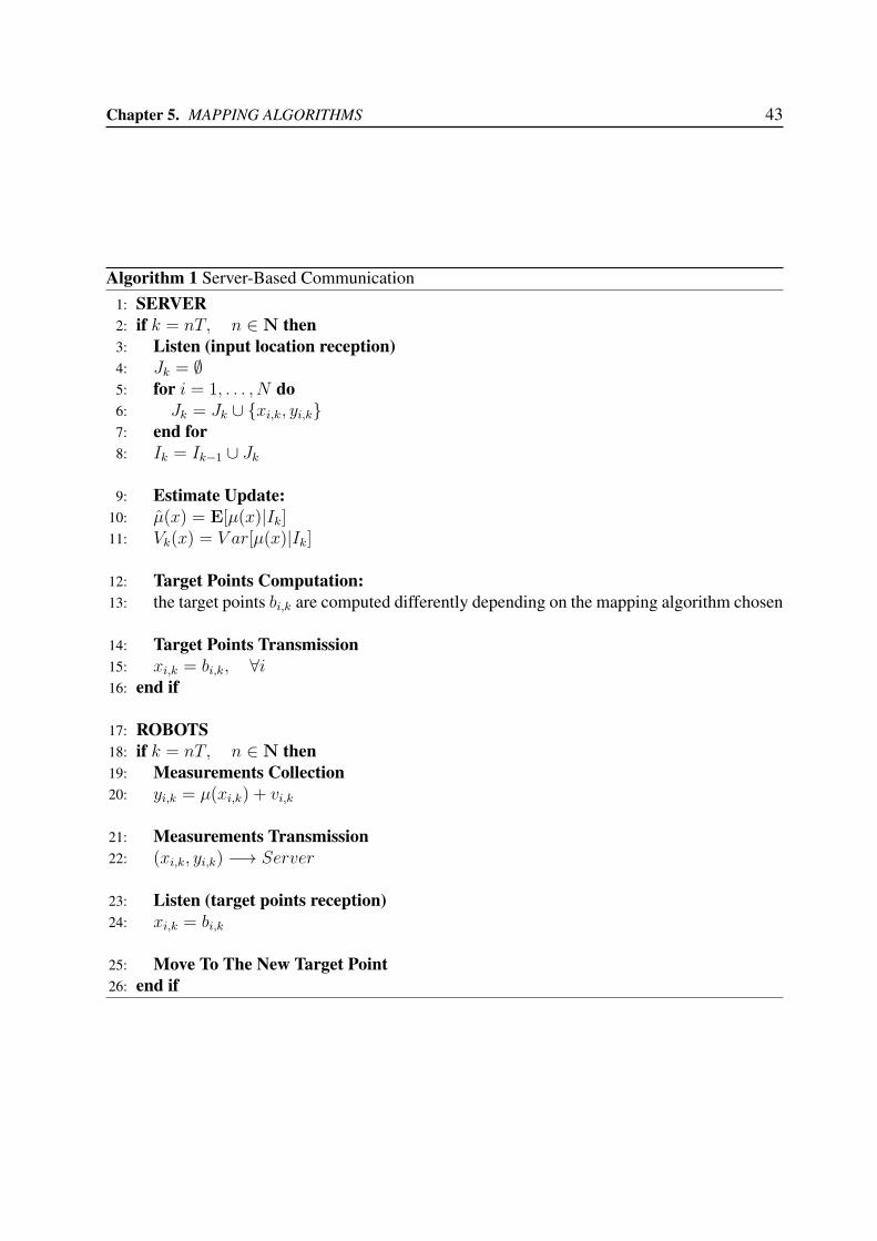
In Algorithm 1 is shown the whole Server-Based communication process where the procedurehave been divided in two parts. The first describes the operations executed by the server, thesecond those executed by the robots.We developed three algorithms in order to calculate in different ways the target points for theagents which are:
1. a randomized selection algorithm;
2. a minimum distance algorithm based on the maximum posterior variance;
3. a distance weighted algorithm based on the posterior variance.
The algorithms return a matrix called ”Target points” where for each row ”i” is stored: in position(i, 1) the number id of the robot we want to send the target point to, in position (i, 2) the x targetpoint coordinate and in position (i, 3) the y target point coordinate.All these algorithms will be explained in the next subsections.
Figure 5.1: The client-server communication architecture considered: the robots can send theirinput locations to the server/base station while the server, after performing all the computation,can send to the robots the target points.
Chapter 5. MAPPING ALGORITHMS 43
Algorithm 1 Server-Based Communication1: SERVER2: if k = nT, n ∈ N then3: Listen (input location reception)4: Jk = ∅5: for i = 1, . . . , N do6: Jk = Jk ∪ {xi,k, yi,k}7: end for8: Ik = Ik−1 ∪ Jk
9: Estimate Update:10: µ(x) = E[µ(x)|Ik]11: Vk(x) = V ar[µ(x)|Ik]
12: Target Points Computation:13: the target points bi,k are computed differently depending on the mapping algorithm chosen
14: Target Points Transmission15: xi,k = bi,k, ∀i16: end if
17: ROBOTS18: if k = nT, n ∈ N then19: Measurements Collection20: yi,k = µ(xi,k) + vi,k
21: Measurements Transmission22: (xi,k, yi,k) −→ Server
23: Listen (target points reception)24: xi,k = bi,k
25: Move To The New Target Point26: end if
44 Implementation of distributed mapping algorithms using mobile Wheelphones
5.3.1 Randomized Selection Algorithm
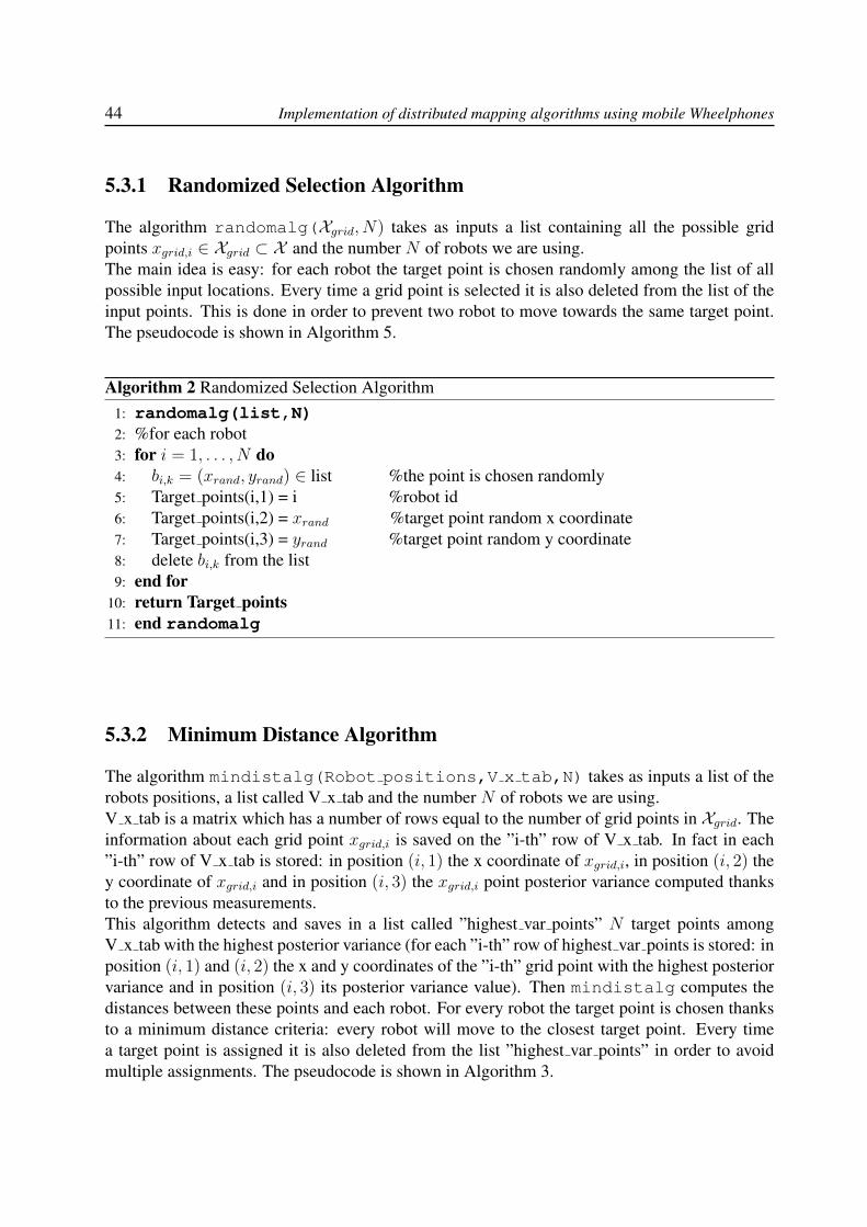
The algorithm randomalg(Xgrid, N) takes as inputs a list containing all the possible gridpoints xgrid,i ∈ Xgrid ⊂ X and the number N of robots we are using.The main idea is easy: for each robot the target point is chosen randomly among the list of allpossible input locations. Every time a grid point is selected it is also deleted from the list of theinput points. This is done in order to prevent two robot to move towards the same target point.The pseudocode is shown in Algorithm 5.
Algorithm 2 Randomized Selection Algorithm1: randomalg(list,N)2: %for each robot3: for i = 1, . . . , N do4: bi,k = (xrand, yrand) ∈ list %the point is chosen randomly5: Target points(i,1) = i %robot id6: Target points(i,2) = xrand %target point random x coordinate7: Target points(i,3) = yrand %target point random y coordinate8: delete bi,k from the list9: end for
10: return Target points11: end randomalg
5.3.2 Minimum Distance Algorithm
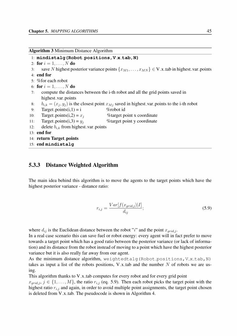
The algorithm mindistalg(Robot positions,V x tab,N) takes as inputs a list of therobots positions, a list called V x tab and the number N of robots we are using.V x tab is a matrix which has a number of rows equal to the number of grid points in Xgrid. Theinformation about each grid point xgrid,i is saved on the ”i-th” row of V x tab. In fact in each”i-th” row of V x tab is stored: in position (i, 1) the x coordinate of xgrid,i, in position (i, 2) they coordinate of xgrid,i and in position (i, 3) the xgrid,i point posterior variance computed thanksto the previous measurements.This algorithm detects and saves in a list called ”highest var points” N target points amongV x tab with the highest posterior variance (for each ”i-th” row of highest var points is stored: inposition (i, 1) and (i, 2) the x and y coordinates of the ”i-th” grid point with the highest posteriorvariance and in position (i, 3) its posterior variance value). Then mindistalg computes thedistances between these points and each robot. For every robot the target point is chosen thanksto a minimum distance criteria: every robot will move to the closest target point. Every timea target point is assigned it is also deleted from the list ”highest var points” in order to avoidmultiple assignments. The pseudocode is shown in Algorithm 3.
Chapter 5. MAPPING ALGORITHMS 45
Algorithm 3 Minimum Distance Algorithm1: mindistalg(Robot positions,V x tab,N)2: for i = 1, . . . , N do3: saveN highest posterior variance points {xM1, . . . , xMN} ∈V x tab in highest var points4: end for5: %for each robot6: for i = 1, . . . , N do7: compute the distances between the i-th robot and all the grid points saved in
highest var points8: bi,k = (xj, yj) is the closest point xMj saved in highest var points to the i-th robot9: Target points(i,1) = i %robot id
10: Target points(i,2) = xj %target point x coordinate11: Target points(i,3) = yj %target point y coordinate12: delete bi,k from highest var points13: end for14: return Target points15: end mindistalg
5.3.3 Distance Weighted Algorithm
The main idea behind this algorithm is to move the agents to the target points which have thehighest posterior variance - distance ratio:
ri,j =V ar[f(xgrid,j)|I]
dij; (5.9)
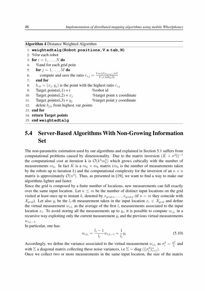
where dij is the Euclidean distance between the robot ”i” and the point xgrid,j .In a real case scenario this can save fuel or robot energy: every agent will in fact prefer to movetowards a target point which has a good ratio between the posterior variance (or lack of informa-tion) and its distance from the robot instead of moving to a point which have the highest posteriorvariance but it is also really far away from our agent.As the minimum distance algorithm, weightedtalg(Robot positions,V x tab,N)takes as input a list of the robots positions, V x tab and the number N of robots we are us-ing.This algorithm thanks to V x tab computes for every robot and for every grid pointxgrid,j , j ∈ {1, . . . ,M}, the ratio ri,j (eq. 5.9). Then each robot picks the target point with thehighest ratio ri,j and again, in order to avoid multiple point assignments, the target point chosenis deleted from V x tab. The pseudocode is shown in Algorithm 4.
46 Implementation of distributed mapping algorithms using mobile Wheelphones
Algorithm 4 Distance Weighted Algorithm1: weightedtalg(Robot positions,V x tab,N)2: %for each robot3: for i = 1, . . . , N do4: %and for each grid poin5: for j = 1, . . . ,M do6: compute and save the ratio ri,j =
V ar[f(xgrid,j)|I]V x tab(j,3)
7: end for8: bi,k = (xj, yj) is the point with the highest ratio ri,j9: Target points(i,1) = i %robot id
10: Target points(i,2) = xj %target point x coordinate11: Target points(i,3) = yj %target point y coordinate12: delete bj,k from highest var points13: end for14: return Target points15: end weightedtalg
5.4 Server-Based Algorithms With Non-Growing InformationSet
The non-parametric estimation used by our algorithms and explained in Section 5.1 suffers fromcomputational problems caused by dimensionality. Due to the matrix inversion (K + σ2I)−1the computational cost at iteration k is O(k3m3
k) which grows cubically with the number ofmeasurements mk. In fact K is a mk × mk matrix (mk is the number of measurements takenby the robots up to iteration k) and the computational complexity for the inversion of an n × nmatrix is approximately O(n3). Thus, as presented in [19], we want to find a way to make ouralgorithms lighter and faster.Since the grid is composed by a finite number of locations, new measurements can fall exactlyover the same input location. Let n ≤ m be the number of distinct input locations on the gridvisited at least once up to instant k, denoted by xgrid,1, . . . , xgrid,n (if n = m they coincide withXgrid). Let also yi be the li-th measurement taken in the input location xi ∈ Xgrid and definethe virtual measurement wi,li as the average of the first li measurements associated to the inputlocation xi. To avoid storing all the measurements up to yi, it is possible to compute wi,li in arecursive way exploiting only the current measurement yi and the previous virtual measurementswi,li−1.In particular, one has:
wi,li =li − 1
liwi,li−1 +
1
liyi (5.10)
Accordingly, we define the variance associated to the virtual measurement wi,li as σ2i = σ2
liand
with Σ a diagonal matrix collecting these noise variances, i.e Σ = diag ({σ2i }ni=1).
Once we collect two or more measurements in the same input location, the size of the matrix
Chapter 5. MAPPING ALGORITHMS 47
K does not vary and it increases only if an input location xgrid,i ∈ X is visited for the firsttime. When all the grid points have been visited at least one time the sampled Kernel K does notchange size anymore.Instead, every time a new measurement is achieved, one has to update the variance matrix Σand the vector with the virtual measurements w = [w1,l1 , . . . , wm,ln ] with n ≤ m. After havingupdated these elements we can compute as usual the function estimate and the posterior varianceusing equations (5.2) and (5.5).
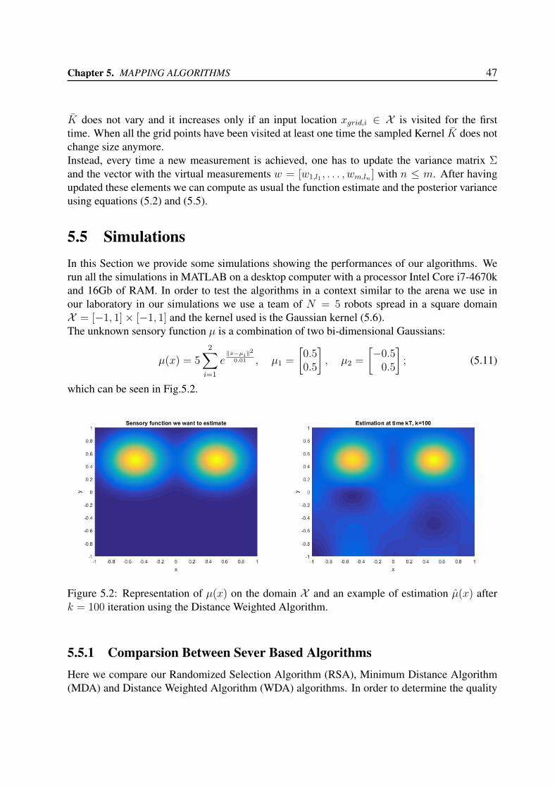
5.5 SimulationsIn this Section we provide some simulations showing the performances of our algorithms. Werun all the simulations in MATLAB on a desktop computer with a processor Intel Core i7-4670kand 16Gb of RAM. In order to test the algorithms in a context similar to the arena we use inour laboratory in our simulations we use a team of N = 5 robots spread in a square domainX = [−1, 1]× [−1, 1] and the kernel used is the Gaussian kernel (5.6).The unknown sensory function µ is a combination of two bi-dimensional Gaussians:
µ(x) = 52∑i=1
e‖x−µi‖
2
0.01 , µ1 =
[0.50.5
], µ2 =
[−0.5
0.5
]; (5.11)
which can be seen in Fig.5.2.
Figure 5.2: Representation of µ(x) on the domain X and an example of estimation µ(x) afterk = 100 iteration using the Distance Weighted Algorithm.
5.5.1 Comparsion Between Sever Based AlgorithmsHere we compare our Randomized Selection Algorithm (RSA), Minimum Distance Algorithm(MDA) and Distance Weighted Algorithm (WDA) algorithms. In order to determine the quality
48 Implementation of distributed mapping algorithms using mobile Wheelphones
of the algorithms the a posterior variance of the points of the set Xgrid and of the set X will beanalyzed. For computational reasons when we compute the a posterior variance of a point x ∈ Xwe consider a grid of 30 equidistant points per side (then the total number of points is p2 = 900).
16 25 36 49 64 81 100
p2
0
0.1
0.2
0.3
0.4
0.5
0.6
0.7
0.8
0.9
1
Ma
x P
oste
rio
r V
aria
nce
N=5, l=2, k=100
Xgrid
, Randomized Selection Algorithm
Xgrid
, Minimum Distance Algorithm
Xgrid
, Distance Weighted Algorithm
X, Randomized Selection Algorithm
X, Minimum Distance Algorithm
X, Distance Weighted Algorithm
Figure 5.3: Comparsion between RSA, MDA and DWA for different total numbers of grid pointsp2g: evolution of the max of the posterior variance averaged over 100 indipendent simulations.
In Fig.5.3 is shown the evolution of the posterior variance for different values of the gridpoints p2g after a number of iterations k = 100. The values of the number of robots used and ofthe side of the squared map are fixed to N = 5 and l = 2 (X = [−1, 1]× [−1, 1]). As we can seethe worst algorithm is the Randomized Selection Algorithm due to its lack of mapping strategywhich performs way worst than the Minimum Distance Algorithm and the Distance WeightedAlgorithm. The best algorithm is the Minimum Distance Algorithm: every robot in fact will ex-plore the points with the highest posterior variance. This helps, in a long run, to keep the averageposterior variance as low as possible. The Distance Weighted Algorithm performs slightly worstthan MDA but it can potentially save a lot of energy/fuel thanks to its conservative strategy. Forevery mapping algorithm the maximum posterior variance found in the set X converges to theone found within the set Xgrid when the value of p2g increases.
In Fig. 5.4 is again shown the evolution of the posterior variance (from 0 to 100 iterations)but this time also the number of grid points is fixed to p2g = 25. Even if the maximum posteriorvariance values found over time for a generic point xi ∈ X are in general high, the maximumposterior variance values for our grid points xgrid,i ∈ Xgrid after 100 iterations are really low(under the 0.1 threshold). This means that for our grid points we have enough information toestimate a value which is really close to the one computed by evaluating the sensory function inthese points and if the number of grid points is reasonable this provides a good estimation of oursensory function (see Fig.5.2).Note that the curves of Figure 5.4 scale with the number of robots. That is increasing the numberof robots, the max of the posterior variance tends to zero more rapidly. In particular the curvesscale as 1√
N. Again, the RSA is the worst of the three algorithms, the MDA is the best and the
DWA preforms similar to the MDA. As we can see from this figure for a low number of iterations
Chapter 5. MAPPING ALGORITHMS 49
0 10 20 30 40 50 60 70 80 90 100
Iteration
0
0.1
0.2
0.3
0.4
0.5
0.6
0.7
0.8
0.9
1
Ma
x P
oste
rio
r V
aria
nce
N=5, p2=25, l=2
Xgrid
, Randomized Selection Algorithm
Xgrid
, Minimum Distance Algorithm
Xgrid
, Distance Weighted Algorithm
X, Randomized Selection Algorithm
X, Minimum Distance Algorithm
X, Distance Weighted Algorithm
Figure 5.4: Comparsion between RSA, MDA and DWA: evolution of the max of the posteriorvariance from 0 to 100 iterations averaged over 100 indipendent simulations.
we want to avoid the Randomized Selection Algorithm, but for number of iteration higher than100 it may be preferable if we don’t have a good computational power since it is light andeasy to implement and it provides a good maximum posterior variance for the grid points. TheDistance Weighted Algorithm is instead preferable if we want to save energy resources like inan emergency or in a military scenario. Lastly if we don’t have any limitations, the MinimumDistance Algorithm is surely the best one.Similar considerations can be made observing Fig. 5.5 where the maximum posterior for somexi ∈ X and for some xgrid,i ∈ Xgrid is computed for different values of N and with a fixednumber of grid points p2g = 25 and l = 2.
0 1 2 3 4 5 6 7 8
N
0
0.1
0.2
0.3
0.4
0.5
0.6
0.7
0.8
0.9
1
Max P
oste
rior
Variance
P2
g=25, l=2, k=100
Xgrid
, Randomized Selection Algorithm
Xgrid
, Minimum Distance Algorithm
Xgrid
, Distance Weighted Algorithm
X, Randomized Selection Algorithm
X, Minimum Distance Algorithm
X, Distance Weighted Algorithm
Figure 5.5: Comparsion between RSA, MDA and DWA for different total numbers of robots N :evolution of the max of the posterior variance averaged over 100 indipendent simulations.
50 Implementation of distributed mapping algorithms using mobile Wheelphones
5.5.2 Comparsion Between Sever Based Algorithms With Non-GrowingInformation Set
In this Section we compare our RSA, MDA and WDA algorithms using an Information set com-puted recursively as shown in Section 5.4. In particular we are going to compare the executiontime of our algorithms with a non growing information set and the same algorithms with a nor-mal stacked information set. In Fig. 5.6 is shown the execution time in seconds of our algorithmsfor a number of iteration k ∈ [0, 100]. As we can see the usage of a non growing information
0 10 20 30 40 50 60 70 80 90 100
Iteration
0
2
4
6
8
10
12
14
16
18
Exe
cu
tio
n T
ime
[s]
N=5, p2
g=25, l=2
RSA
MDA
DWA
RSA-NGIS
MDA-NGIS
DWA-NGIS
Figure 5.6: Comparsion between RSA, MDA, DWA and the same version of these algorithmsusing a non-growing information set: evolution of the execution time averaged over 100 indipen-dent simulations.
set makes the evolution of the execution time for a varying value of iterations k almost linearcompared to the evolution of the execution time of our algorithms with a ”normal” informationset which has an exponential behavior. Therefore for a real time application the usage of a nongrowing information set (NGIS) is strongly recommended.This last statement is reinforced by what we can see in Fig. 5.7 where the evolution of the max-imum posterior variance is printed for different iterations values and for both versions of thealgorithms. This image proves that the NGIS version of our algorithms performs similar to thenormal version of the same algorithms but, using a non growing information set, we have a muchfaster execution time.This faster execution time allows us to test our algorithms for a higher value of iterations andgrid points. In Fig. 5.8 is again shown the evolution of the posterior variance (from 0 to 100iterations) but with a number of grid points fixed to p2g = 64. From this picture we can observethat the maximum posterior found for a generic xi ∈ X is decreasing when also the numberof iteration is increasing. This means that with a more dense grid and with an high number ofiterations we will have a more reliable knowledge of our sensory function for a point xi outsidethe grid set Xgrid.
Chapter 5. MAPPING ALGORITHMS 51
0 10 20 30 40 50 60 70 80 90 100
Iteration
0
0.1
0.2
0.3
0.4
0.5
0.6
0.7
0.8
0.9
1
Ma
x P
oste
rio
r V
aria
nce
N=5, p2
g=64, l=2, NGIM
Xgrid
, RSA
Xgrid
, MDA
Xgrid
, DWA
Xgrid
, RSA-NGIS
Xgrid
, MDA-NGIS
Xgrid
, DWA-NGIS
Figure 5.7: Comparsion between RSA, MDA, DWA and the same version of these algorithmsusing a non-growing information set: evolution of the max of the posterior variance from 0 to100 iterations averaged over 100 indipendent simulations.
0 50 100 150 200 250 300 350 400
Iteration
0
0.1
0.2
0.3
0.4
0.5
0.6
0.7
0.8
0.9
1
Ma
x P
oste
rio
r V
aria
nce
N=5, p2
g=64, l=2
Xgrid
, RSA-NGIS
Xgrid
, MDA-NGIS
Xgrid
, DWA-NGIS
X, RSA-NGIS
X, MDA-NGIS
X, DWA-NGIS
Figure 5.8: Comparsion between RSA-NGIS, MDA-NGIS and DWA-NGIS: evolution of themax of the posterior variance for both the sets X and Xgrid from 0 to 400 iterations averagedover 100 indipendent simulations.

Chapter 6
WHEELPHONE IMPLEMENTATION
To implement our algorithms using several Wheelphone robots we need to have a precise posi-tion value of the robot within the map. The odometry we found in Section 4.1.4 is unsuccessfulin this sense for many reasons. First of all the Wheelphone does not have a true wheel encoderbut it estimates the wheels linear velocity thanks to the voltage applied to the two DC motors.This leads to a raw velocity estimation and thus to a position estimation affected by errors. Inaddition to this problem wheel slippage, carpet ”springiness” and uneven floors can affect theodometry accuracy. In Fig. 6.1 is depicted a test we did to see the odometry error we weretalking about. The robot has been positioned on the origin of the global reference frame and wegave to the agent four points (x1 = (0.5, 0), x2 = (0.5, 0.5), x3 = (0, 0.5) and x4 = (0, 0)) tovisit. The blue line represents the ideal trajectory the robot should have done computed thanksto its odomoetry while the red line is the trajectory the robot actually did (recorded thanks to themotion capture system) because of the problem we have just discussed. As we can see after threepoint to point movements the robot totally failed to reach the final destination.
-0.2 -0.1 0 0.1 0.2 0.3 0.4 0.5 0.6 0.7
x [m]
-0.1
0
0.1
0.2
0.3
0.4
0.5
0.6
0.7
y [
m]
Odometry Error
real odometry
ideal internal odometry
reference points
Figure 6.1: Robot trajectories test: the blue line is the ideal path computed thanks to theodomoetry while the red line is the real trajectory the robot did.
53
54 Implementation of distributed mapping algorithms using mobile Wheelphones
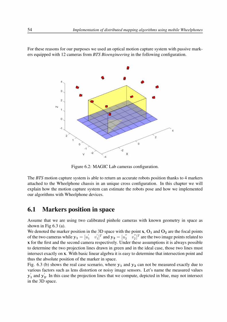
For these reasons for our purposes we used an optical motion capture system with passive mark-ers equipped with 12 cameras from BTS Bioengineering in the following configuration.
Figure 6.2: MAGIC Lab cameras configuration.
The BTS motion capture system is able to return an accurate robots position thanks to 4 markersattached to the Wheelphone chassis in an unique cross configuration. In this chapter we willexplain how the motion capture system can estimate the robots pose and how we implementedour algorithms with Wheelphone devices.
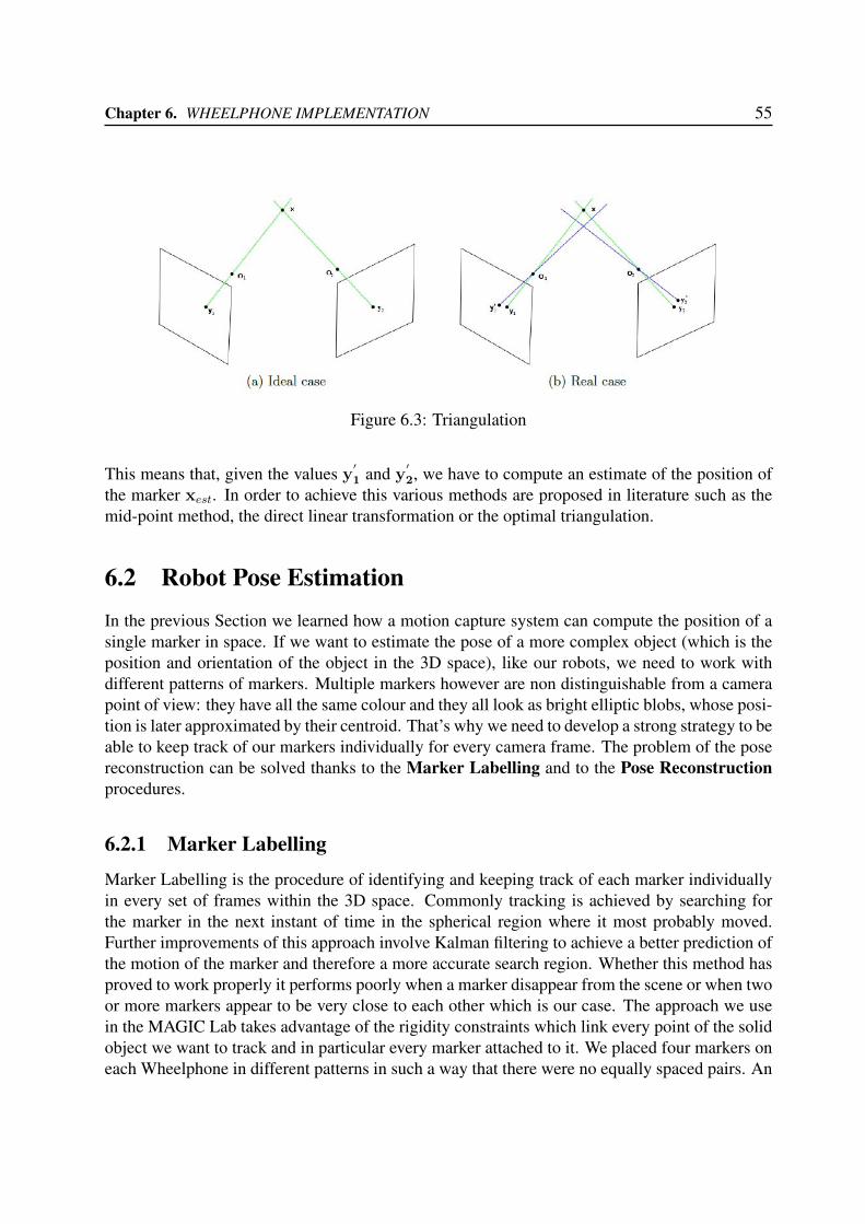
6.1 Markers position in spaceAssume that we are using two calibrated pinhole cameras with known geometry in space asshown in Fig 6.3 (a).We denoted the marker position in the 3D space with the point x, O1 and O2 are the focal pointsof the two cameras while y1 = [u
′1 v
′1]T and y2 = [u
′′2 v
′′2 ]T are the two image points related to
x for the first and the second camera respectively. Under these assumptions it is always possibleto determine the two projection lines drawn in green and in the ideal case, those two lines mustintersect exactly on x. With basic linear algebra it is easy to determine that intersection point andthus the absolute position of the marker in space.Fig. 6.3 (b) shows the real case scenario, where y1 and y2 can not be measured exactly due tovarious factors such as lens distortion or noisy image sensors. Let’s name the measured valuesy′1 and y
′2. In this case the projection lines that we compute, depicted in blue, may not intersect
in the 3D space.
Chapter 6. WHEELPHONE IMPLEMENTATION 55
Figure 6.3: Triangulation
This means that, given the values y′1 and y′2, we have to compute an estimate of the position of
the marker xest. In order to achieve this various methods are proposed in literature such as themid-point method, the direct linear transformation or the optimal triangulation.
6.2 Robot Pose EstimationIn the previous Section we learned how a motion capture system can compute the position of asingle marker in space. If we want to estimate the pose of a more complex object (which is theposition and orientation of the object in the 3D space), like our robots, we need to work withdifferent patterns of markers. Multiple markers however are non distinguishable from a camerapoint of view: they have all the same colour and they all look as bright elliptic blobs, whose posi-tion is later approximated by their centroid. That’s why we need to develop a strong strategy to beable to keep track of our markers individually for every camera frame. The problem of the posereconstruction can be solved thanks to the Marker Labelling and to the Pose Reconstructionprocedures.
6.2.1 Marker Labelling
Marker Labelling is the procedure of identifying and keeping track of each marker individuallyin every set of frames within the 3D space. Commonly tracking is achieved by searching forthe marker in the next instant of time in the spherical region where it most probably moved.Further improvements of this approach involve Kalman filtering to achieve a better prediction ofthe motion of the marker and therefore a more accurate search region. Whether this method hasproved to work properly it performs poorly when a marker disappear from the scene or when twoor more markers appear to be very close to each other which is our case. The approach we usein the MAGIC Lab takes advantage of the rigidity constraints which link every point of the solidobject we want to track and in particular every marker attached to it. We placed four markers oneach Wheelphone in different patterns in such a way that there were no equally spaced pairs. An
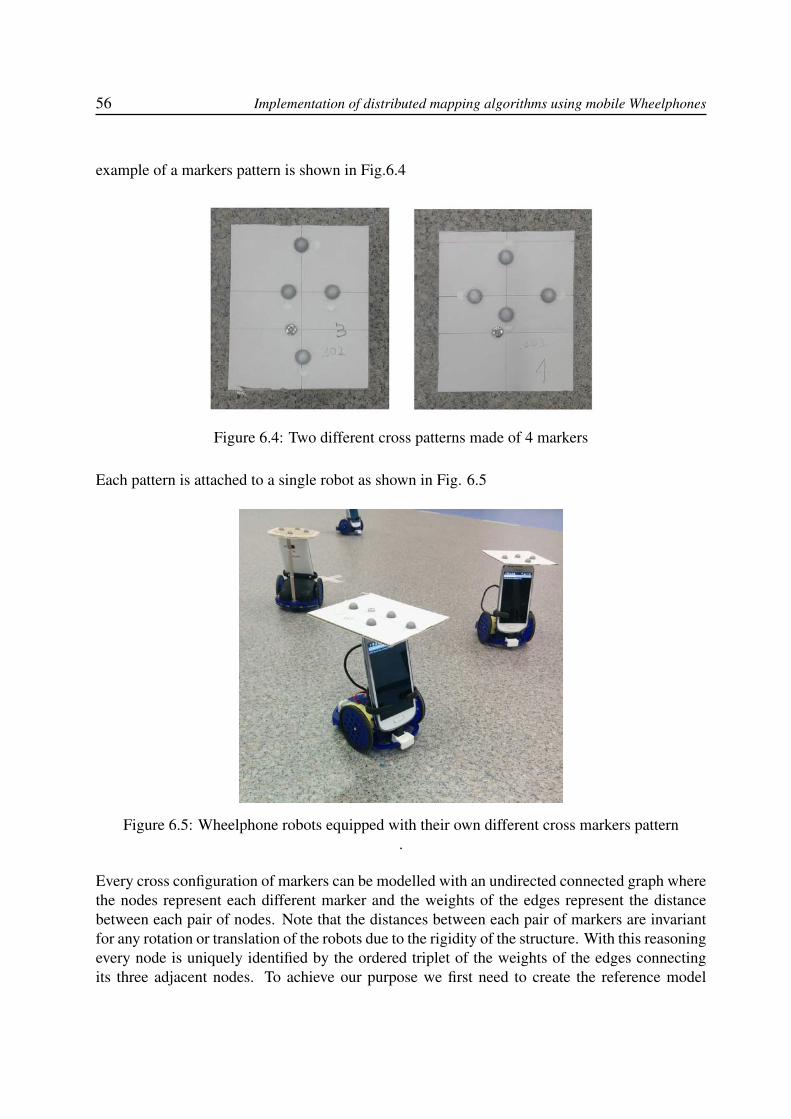
56 Implementation of distributed mapping algorithms using mobile Wheelphones
example of a markers pattern is shown in Fig.6.4
Figure 6.4: Two different cross patterns made of 4 markers
Each pattern is attached to a single robot as shown in Fig. 6.5
Figure 6.5: Wheelphone robots equipped with their own different cross markers pattern.
Every cross configuration of markers can be modelled with an undirected connected graph wherethe nodes represent each different marker and the weights of the edges represent the distancebetween each pair of nodes. Note that the distances between each pair of markers are invariantfor any rotation or translation of the robots due to the rigidity of the structure. With this reasoningevery node is uniquely identified by the ordered triplet of the weights of the edges connectingits three adjacent nodes. To achieve our purpose we first need to create the reference model
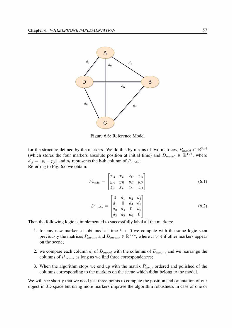
Chapter 6. WHEELPHONE IMPLEMENTATION 57
Figure 6.6: Reference Model
for the structure defined by the markers. We do this by means of two matrices, Pmodel ∈ R3×4
(which stores the four markers absolute position at initial time) and Dmodel ∈ R4×4, wheredij = ‖pi − pj‖ and pk represents the k-th column of Pmodel.Referring to Fig. 6.6 we obtain:
Pmodel =
xA xB xC xDyA yB yC yDzA xB zC zD
(6.1)
Dmodel =
0 d1 d2 d3d1 0 d4 d5d2 d4 0 d6d3 d5 d6 0
(6.2)
Then the following logic is implemented to successfully label all the markers:
1. for any new marker set obtained at time t > 0 we compute with the same logic seenpreviously the matrices Pmeans and Dmeans ∈ Rn×n, where n > 4 if other markers appearon the scene;
2. we compare each column di of Dmodel with the columns of Dmeans and we rearrange thecolumns of Pmeans as long as we find three correspondences;
3. When the algorithm stops we end up with the matrix Pmeas ordered and polished of thecolumns corresponding to the markers on the scene which didnt belong to the model.
We will see shortly that we need just three points to compute the position and orientation of ourobject in 3D space but using more markers improve the algorithm robustness in case of one or
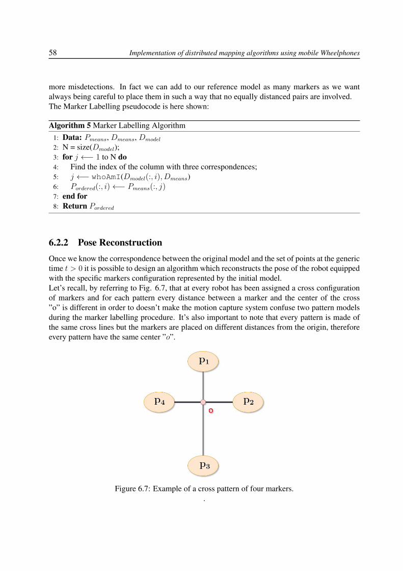
58 Implementation of distributed mapping algorithms using mobile Wheelphones
more misdetections. In fact we can add to our reference model as many markers as we wantalways being careful to place them in such a way that no equally distanced pairs are involved.The Marker Labelling pseudocode is here shown:
Algorithm 5 Marker Labelling Algorithm1: Data: Pmeans, Dmeans, Dmodel
2: N = size(Dmodel);3: for j ←− 1 to N do4: Find the index of the column with three correspondences;5: j ←− whoAmI(Dmodel(:, i), Dmeans)6: Pordered(:, i)←− Pmeans(:, j)7: end for8: Return Pordered
6.2.2 Pose ReconstructionOnce we know the correspondence between the original model and the set of points at the generictime t > 0 it is possible to design an algorithm which reconstructs the pose of the robot equippedwith the specific markers configuration represented by the initial model.Let’s recall, by referring to Fig. 6.7, that at every robot has been assigned a cross configurationof markers and for each pattern every distance between a marker and the center of the cross”o” is different in order to doesn’t make the motion capture system confuse two pattern modelsduring the marker labelling procedure. It’s also important to note that every pattern is made ofthe same cross lines but the markers are placed on different distances from the origin, thereforeevery pattern have the same center ”o”.
Figure 6.7: Example of a cross pattern of four markers..
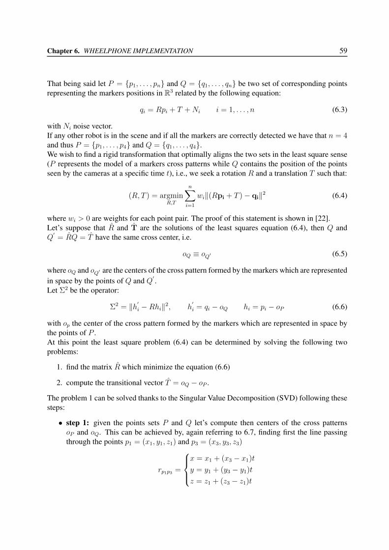
Chapter 6. WHEELPHONE IMPLEMENTATION 59
That being said let P = {p1, . . . , pn} and Q = {q1, . . . , qn} be two set of corresponding pointsrepresenting the markers positions in R3 related by the following equation:
qi = Rpi + T +Ni i = 1, . . . , n (6.3)
with Ni noise vector.If any other robot is in the scene and if all the markers are correctly detected we have that n = 4and thus P = {p1, . . . , p4} and Q = {q1, . . . , q4}.We wish to find a rigid transformation that optimally aligns the two sets in the least square sense(P represents the model of a markers cross patterns while Q contains the position of the pointsseen by the cameras at a specific time t), i.e., we seek a rotation R and a translation T such that:
(R, T ) = argminR,T
n∑i=1
wi‖(Rpi + T )− qi‖2 (6.4)
where wi > 0 are weights for each point pair. The proof of this statement is shown in [22].Let’s suppose that R and T are the solutions of the least squares equation (6.4), then Q andQ′= RQ = T have the same cross center, i.e.
oQ ≡ oQ′ (6.5)
where oQ and oQ′ are the centers of the cross pattern formed by the markers which are representedin space by the points of Q and Q′ .Let Σ2 be the operator:
Σ2 = ‖h′i −Rhi‖2, h′
i = qi − oQ hi = pi − oP (6.6)
with op the center of the cross pattern formed by the markers which are represented in space bythe points of P .At this point the least square problem (6.4) can be determined by solving the following twoproblems:
1. find the matrix R which minimize the equation (6.6)
2. compute the transitional vector T = oQ − oP .
The problem 1 can be solved thanks to the Singular Value Decomposition (SVD) following thesesteps:
• step 1: given the points sets P and Q let’s compute then centers of the cross patternsoP and oQ. This can be achieved by, again referring to 6.7, finding first the line passingthrough the points p1 = (x1, y1, z1) and p3 = (x3, y3, z3)
rp1p3 =
x = x1 + (x3 − x1)ty = y1 + (y3 − y1)tz = z1 + (z3 − z1)t
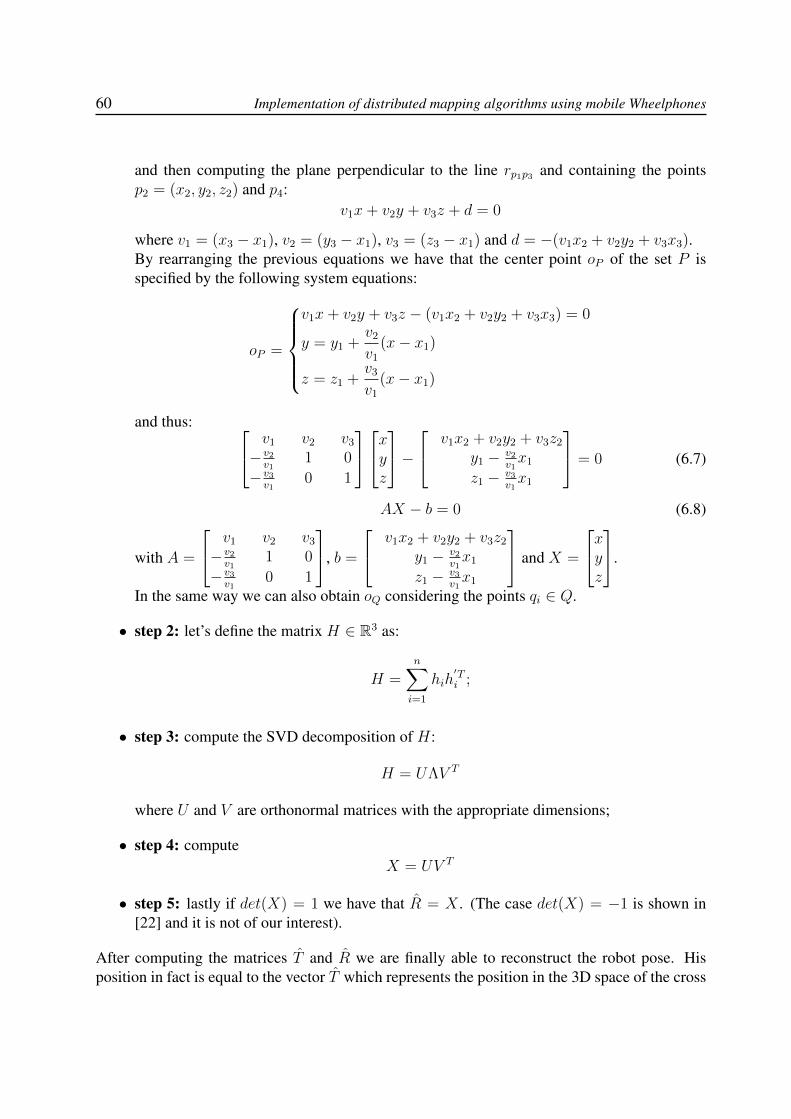
60 Implementation of distributed mapping algorithms using mobile Wheelphones
and then computing the plane perpendicular to the line rp1p3 and containing the pointsp2 = (x2, y2, z2) and p4:
v1x+ v2y + v3z + d = 0
where v1 = (x3 − x1), v2 = (y3 − x1), v3 = (z3 − x1) and d = −(v1x2 + v2y2 + v3x3).By rearranging the previous equations we have that the center point oP of the set P isspecified by the following system equations:
oP =
v1x+ v2y + v3z − (v1x2 + v2y2 + v3x3) = 0
y = y1 +v2v1
(x− x1)
z = z1 +v3v1
(x− x1)
and thus: v1 v2 v3−v2v1
1 0
−v3v1
0 1
xyz
− v1x2 + v2y2 + v3z2
y1 − v2v1x1
z1 − v3v1x1
= 0 (6.7)
AX − b = 0 (6.8)
with A =
v1 v2 v3−v2v1
1 0
−v3v1
0 1
, b =
v1x2 + v2y2 + v3z2y1 − v2
v1x1
z1 − v3v1x1
and X =
xyz
.
In the same way we can also obtain oQ considering the points qi ∈ Q.
• step 2: let’s define the matrix H ∈ R3 as:
H =n∑i=1
hih′Ti ;
• step 3: compute the SVD decomposition of H:
H = UΛV T
where U and V are orthonormal matrices with the appropriate dimensions;
• step 4: computeX = UV T
• step 5: lastly if det(X) = 1 we have that R = X . (The case det(X) = −1 is shown in[22] and it is not of our interest).
After computing the matrices T and R we are finally able to reconstruct the robot pose. Hisposition in fact is equal to the vector T which represents the position in the 3D space of the cross
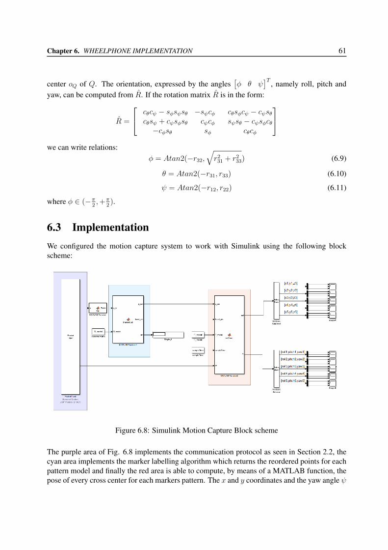
Chapter 6. WHEELPHONE IMPLEMENTATION 61
center oQ of Q. The orientation, expressed by the angles[φ θ ψ
]T , namely roll, pitch andyaw, can be computed from R. If the rotation matrix R is in the form:
R =
cθcψ − sφsψsθ −sψcφ cθsφcψ − cψsθcθsψ + cψsφsθ cψcφ sψsθ − cψsφcθ−cφsθ sφ cθcφ
we can write relations:
φ = Atan2(−r32,√r231 + r233) (6.9)
θ = Atan2(−r31, r33) (6.10)
ψ = Atan2(−r12, r22) (6.11)
where φ ∈ (−π2,+π
2).
6.3 ImplementationWe configured the motion capture system to work with Simulink using the following blockscheme:
Figure 6.8: Simulink Motion Capture Block scheme
The purple area of Fig. 6.8 implements the communication protocol as seen in Section 2.2, thecyan area implements the marker labelling algorithm which returns the reordered points for eachpattern model and finally the red area is able to compute, by means of a MATLAB function, thepose of every cross center for each markers pattern. The x and y coordinates and the yaw angle ψ
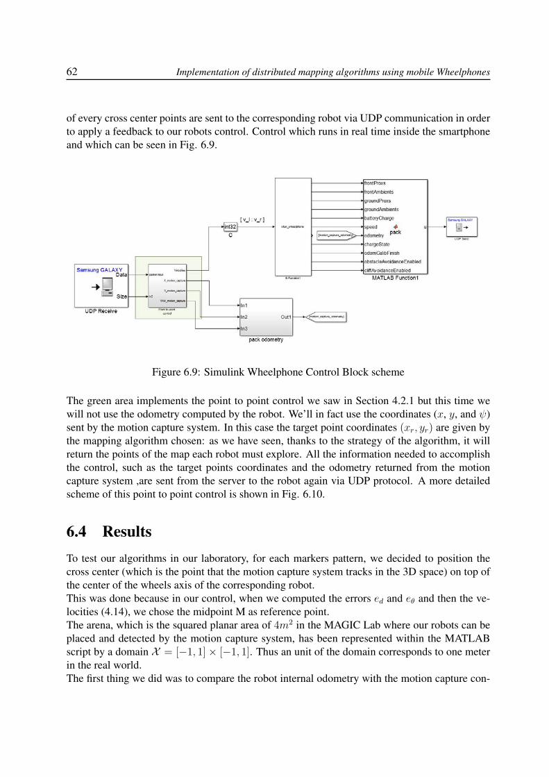
62 Implementation of distributed mapping algorithms using mobile Wheelphones
of every cross center points are sent to the corresponding robot via UDP communication in orderto apply a feedback to our robots control. Control which runs in real time inside the smartphoneand which can be seen in Fig. 6.9.
Figure 6.9: Simulink Wheelphone Control Block scheme
The green area implements the point to point control we saw in Section 4.2.1 but this time wewill not use the odometry computed by the robot. We’ll in fact use the coordinates (x, y, and ψ)sent by the motion capture system. In this case the target point coordinates (xr, yr) are given bythe mapping algorithm chosen: as we have seen, thanks to the strategy of the algorithm, it willreturn the points of the map each robot must explore. All the information needed to accomplishthe control, such as the target points coordinates and the odometry returned from the motioncapture system ,are sent from the server to the robot again via UDP protocol. A more detailedscheme of this point to point control is shown in Fig. 6.10.
6.4 ResultsTo test our algorithms in our laboratory, for each markers pattern, we decided to position thecross center (which is the point that the motion capture system tracks in the 3D space) on top ofthe center of the wheels axis of the corresponding robot.This was done because in our control, when we computed the errors ed and eθ and then the ve-locities (4.14), we chose the midpoint M as reference point.The arena, which is the squared planar area of 4m2 in the MAGIC Lab where our robots can beplaced and detected by the motion capture system, has been represented within the MATLABscript by a domain X = [−1, 1]× [−1, 1]. Thus an unit of the domain corresponds to one meterin the real world.The first thing we did was to compare the robot internal odometry with the motion capture con-
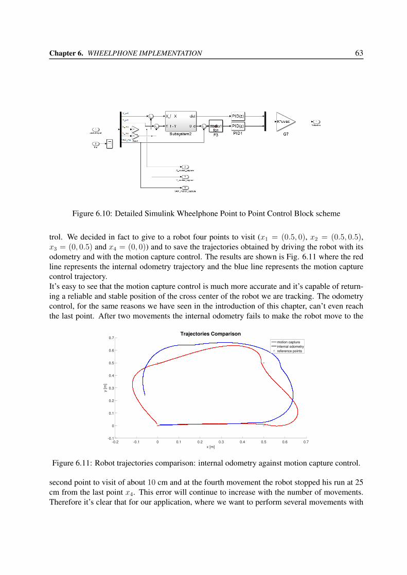
Chapter 6. WHEELPHONE IMPLEMENTATION 63
Figure 6.10: Detailed Simulink Wheelphone Point to Point Control Block scheme
trol. We decided in fact to give to a robot four points to visit (x1 = (0.5, 0), x2 = (0.5, 0.5),x3 = (0, 0.5) and x4 = (0, 0)) and to save the trajectories obtained by driving the robot with itsodometry and with the motion capture control. The results are shown is Fig. 6.11 where the redline represents the internal odometry trajectory and the blue line represents the motion capturecontrol trajectory.It’s easy to see that the motion capture control is much more accurate and it’s capable of return-ing a reliable and stable position of the cross center of the robot we are tracking. The odometrycontrol, for the same reasons we have seen in the introduction of this chapter, can’t even reachthe last point. After two movements the internal odometry fails to make the robot move to the
-0.2 -0.1 0 0.1 0.2 0.3 0.4 0.5 0.6 0.7
x [m]
-0.1
0
0.1
0.2
0.3
0.4
0.5
0.6
0.7
y [
m]
Trajectories Comparison
motion capture
internal odometry
reference points
Figure 6.11: Robot trajectories comparison: internal odometry against motion capture control.
second point to visit of about 10 cm and at the fourth movement the robot stopped his run at 25cm from the last point x4. This error will continue to increase with the number of movements.Therefore it’s clear that for our application, where we want to perform several movements with
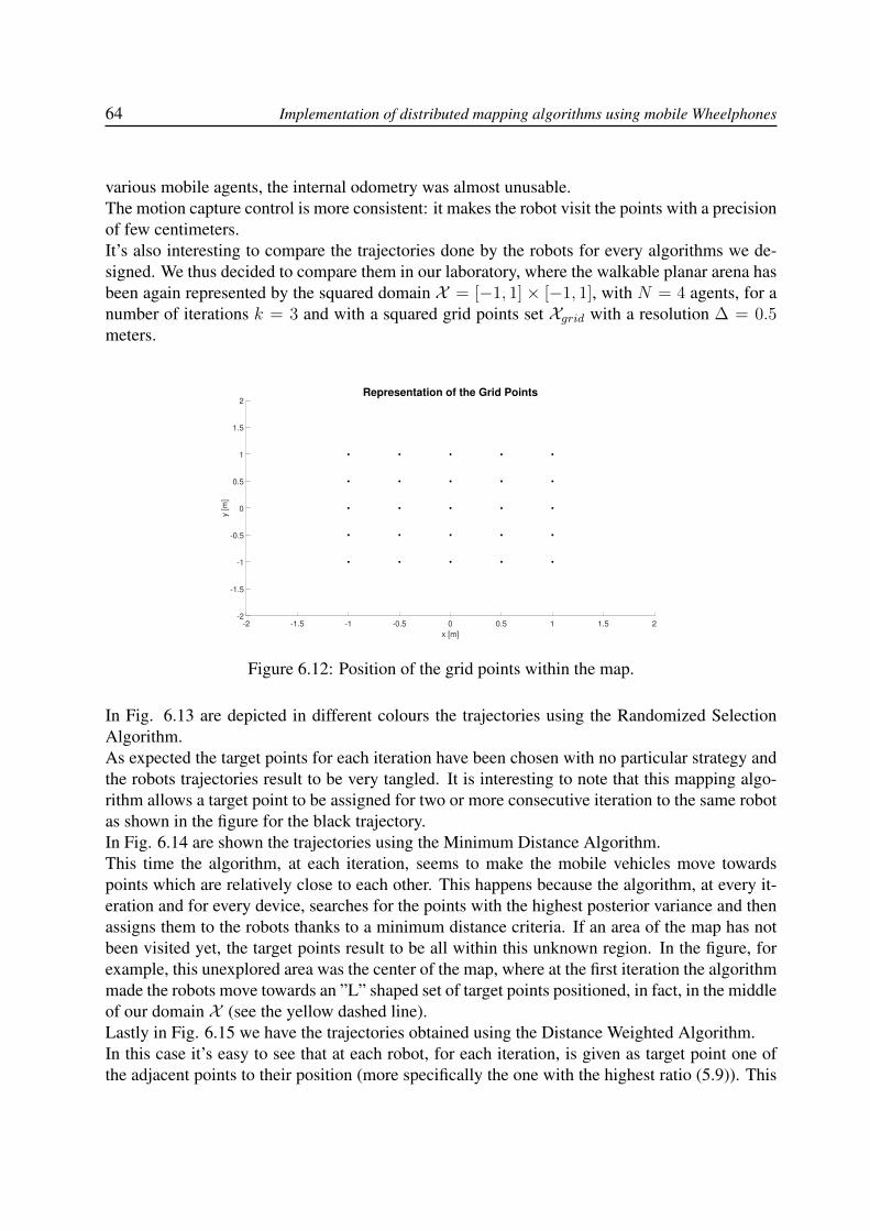
64 Implementation of distributed mapping algorithms using mobile Wheelphones
various mobile agents, the internal odometry was almost unusable.The motion capture control is more consistent: it makes the robot visit the points with a precisionof few centimeters.It’s also interesting to compare the trajectories done by the robots for every algorithms we de-signed. We thus decided to compare them in our laboratory, where the walkable planar arena hasbeen again represented by the squared domain X = [−1, 1] × [−1, 1], with N = 4 agents, for anumber of iterations k = 3 and with a squared grid points set Xgrid with a resolution ∆ = 0.5meters.
-2 -1.5 -1 -0.5 0 0.5 1 1.5 2
x [m]
-2
-1.5
-1
-0.5
0
0.5
1
1.5
2
y [
m]
Representation of the Grid Points
Figure 6.12: Position of the grid points within the map.
In Fig. 6.13 are depicted in different colours the trajectories using the Randomized SelectionAlgorithm.As expected the target points for each iteration have been chosen with no particular strategy andthe robots trajectories result to be very tangled. It is interesting to note that this mapping algo-rithm allows a target point to be assigned for two or more consecutive iteration to the same robotas shown in the figure for the black trajectory.In Fig. 6.14 are shown the trajectories using the Minimum Distance Algorithm.This time the algorithm, at each iteration, seems to make the mobile vehicles move towardspoints which are relatively close to each other. This happens because the algorithm, at every it-eration and for every device, searches for the points with the highest posterior variance and thenassigns them to the robots thanks to a minimum distance criteria. If an area of the map has notbeen visited yet, the target points result to be all within this unknown region. In the figure, forexample, this unexplored area was the center of the map, where at the first iteration the algorithmmade the robots move towards an ”L” shaped set of target points positioned, in fact, in the middleof our domain X (see the yellow dashed line).Lastly in Fig. 6.15 we have the trajectories obtained using the Distance Weighted Algorithm.In this case it’s easy to see that at each robot, for each iteration, is given as target point one ofthe adjacent points to their position (more specifically the one with the highest ratio (5.9)). This
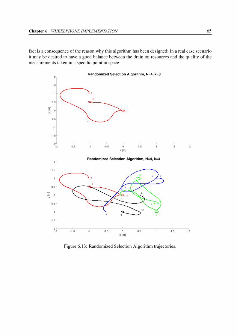
Chapter 6. WHEELPHONE IMPLEMENTATION 65
fact is a consequence of the reason why this algorithm has been designed: in a real case scenarioit may be desired to have a good balance between the drain on resources and the quality of themeasurements taken in a specific point in space.
-2 -1.5 -1 -0.5 0 0.5 1 1.5 2
x [m]
-2
-1.5
-1
-0.5
0
0.5
1
1.5
2
y [
m]
Randomized Selection Algorithm, N=4, k=3
1
3
0
2
-2 -1.5 -1 -0.5 0 0.5 1 1.5 2
x [m]
-2
-1.5
-1
-0.5
0
0.5
1
1.5
2
y [
m]
Randomized Selection Algorithm, N=4, k=3
1
1
3
1
3
0
02
0
3
1,2
3
022
Figure 6.13: Randomized Selection Algorithm trajectories.
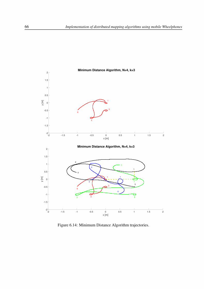
66 Implementation of distributed mapping algorithms using mobile Wheelphones
-2 -1.5 -1 -0.5 0 0.5 1 1.5 2
x [m]
-2
-1.5
-1
-0.5
0
0.5
1
1.5
2
y [
m]
Minimum Distance Algorithm, N=4, k=3
2
0
3
1
-2 -1.5 -1 -0.5 0 0.5 1 1.5 2
x [m]
-2
-1.5
-1
-0.5
0
0.5
1
1.5
2
y [
m]
Minimum Distance Algorithm, N=4, k=3
2
1
3
0
2
0
3
3
1 1
1
2
0
3
2
0
Figure 6.14: Minimum Distance Algorithm trajectories.
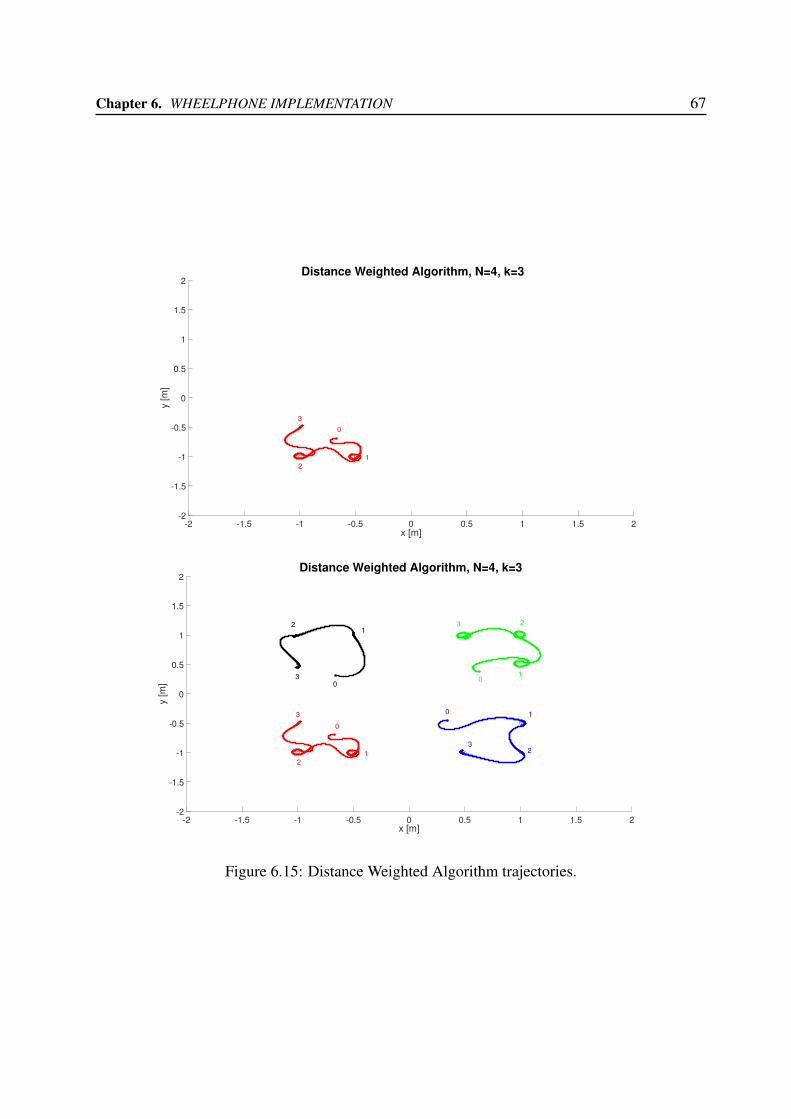
Chapter 6. WHEELPHONE IMPLEMENTATION 67
-2 -1.5 -1 -0.5 0 0.5 1 1.5 2x [m]
-2
-1.5
-1
-0.5
0
0.5
1
1.5
2
y [
m]
Distance Weighted Algorithm, N=4, k=3
2
0
1
3
-2 -1.5 -1 -0.5 0 0.5 1 1.5 2x [m]
-2
-1.5
-1
-0.5
0
0.5
1
1.5
2
y [
m]
Distance Weighted Algorithm, N=4, k=3
1
2
3
30
01
23
0 1
2321
0
Figure 6.15: Distance Weighted Algorithm trajectories.

Chapter 7
CONCLUSIONS
In this dissertation we proposed and applied with real differential drive agents some mappingalgorithms based on the article in [19].
In Chapter 3 we explained how we developed a stable driver interface needed to control, thanks tothe MATLAB/Simulink environment, our Wheelphone devices. The drivers file have been writ-ten with the intent of don’t overwork the computational capabilities of the CPU of the robots.
In Chapter 5 we addressed the problem of mapping with multiple robots assuming the sensoryfield which approximate the sensory distribution of events is unknown. We proposed three algo-rithms in the context of a client-server architecture which is guaranteed to asymptotically exactlyestimate the unknown sensory function. We also provided an alternative version of the algo-rithms which, using a non growing information matrix I , have dramatic reduction in terms ofmemory and CPU requirements. We also tested the performance of the algorithms via extensivenumerical simulations and we tried to find the right application for each algorithm.
In Chapter 6 we showed how we tested our algorithms in a real case scenario. The server knowsthe position of the robots thanks to a motion capture system which, using different cross shapedmarkers patterns, returns the pose of our agents in the 3D space. This is possible by utilizing theMarker Labelling and the Pose Reconstruction algorithms. The point to point control which therobots use in order to move towards their target points is also proposed. This control, thanks tothe work we explained in Chapter 3, runs in real time as an android app on the phone attached tothe wheelphone mobile base. We also commented some test we did in our MAGIC Lab wherewe compared the robots trajectories of each algorithm.
7.1 Future DevelopmentsSeveral developments should be studied in the future. Here some examples are written.
• Developing the same three algorithms we saw in this thesis but in a Distributed Gossipcase where, without the help of a server computer, the target points are computed by the
69
70 Implementation of distributed mapping algorithms using mobile Wheelphones
robots which are capable of exchanging information with each other.
• Implementing, with true wheeled devices, some algorithms capable of resolving the prob-lem of simultaneously mapping and coverage.
• Making the mapping algorithms work in the case of a complex environment with insur-mountable obstacles. This problem needs to be solved with a collision avoidance and wallfollowing algorithms. This are algorithms which need a reliable hardware such as somegood proximity sensors.

Appendices
71

Appendix A
Target Language Compiler
Target Language Compiler (TLC) is an is an advanced feature within Simulink Coder. It allowsyou to customize generated code in order to produce platform-specific code or incorporate yourown algorithmic changes for performance, code size or compatibility with existing methods thatyou prefer to maintain. It provides:
• A set of TLC files corresponding to a subset of the provided Simulink blocks.
• TLC files for model-wide information that specify header and parameter information.
The TLC files are ASCII files that explicitly control the way code is generated. By editing aTLC file, we can alter the way code is generated (we can produce ANSI C or C++ code). TheSimulink Coder invokes The Target Language Compiler after the Simulink model is compiledinto an intermediate form (model.rtw) that is suitable for generating code. The TLC thentransforms this representation file of the diagram into C or C++ code. The model.rtw filecontains a partial representation of the model describing the execution of the block diagram in ahigh-level language. After reading the model.rtw file the target Language Compiler generatesits code based on target files, which specify particular code for each block, and model wide fileswhich specify the overall code style. To create a target-specific application, the code generatorrequires a template makefile that specifies a C or C++ compiler options for the build process.The code generator transform the template makefile into a target makefile (model.mk). Theoverall procedure is shown in Fig.A.1.The TLC is really helpful when we must:
• Change the way code is generated for a particular Simulink block
• Inline S-functions in our model
• Modify the way code is generated in a global sense
• Perform a large scale customization of the generated code, for example, if you need tooutput the code in a language other than C
73
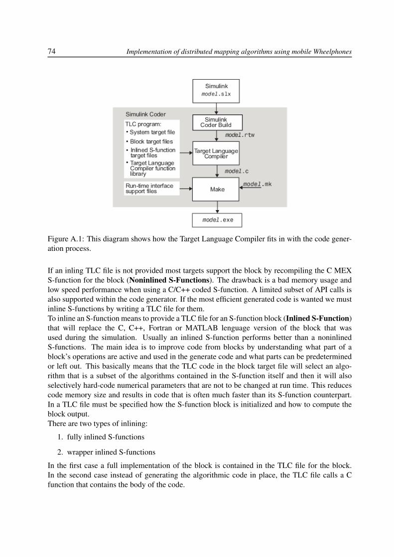
74 Implementation of distributed mapping algorithms using mobile Wheelphones
Figure A.1: This diagram shows how the Target Language Compiler fits in with the code gener-ation process.
If an inling TLC file is not provided most targets support the block by recompiling the C MEXS-function for the block (Noninlined S-Functions). The drawback is a bad memory usage andlow speed performance when using a C/C++ coded S-function. A limited subset of API calls isalso supported within the code generator. If the most efficient generated code is wanted we mustinline S-functions by writing a TLC file for them.To inline an S-function means to provide a TLC file for an S-function block (Inlined S-Function)that will replace the C, C++, Fortran or MATLAB lenguage version of the block that wasused during the simulation. Usually an inlined S-function performs better than a noninlinedS-functions. The main idea is to improve code from blocks by understanding what part of ablock’s operations are active and used in the generate code and what parts can be predeterminedor left out. This basically means that the TLC code in the block target file will select an algo-rithm that is a subset of the algorithms contained in the S-function itself and then it will alsoselectively hard-code numerical parameters that are not to be changed at run time. This reducescode memory size and results in code that is often much faster than its S-function counterpart.In a TLC file must be specified how the S-function block is initialized and how to compute theblock output.There are two types of inlining:
1. fully inlined S-functions
2. wrapper inlined S-functions
In the first case a full implementation of the block is contained in the TLC file for the block.In the second case instead of generating the algorithmic code in place, the TLC file calls a Cfunction that contains the body of the code.
Appendix B
Tikhonov Regularization
Let f : X −→ R denote an unknown deterministic function defined on the compact X ∈ Rd.Assume to have a measurement model as the following:
y = f(x) + v,
with v white noise and x a generic input location (x ∈ X ).Given the data set {xi, yi}Ni=1, where N is the number of measurements collected, one of themost used approaches to estimate f is the so called Tikhonov Regularization, which relies on theTikhonov regularization theory. The hypothesis space is typically given by a reproducing kernelHilbert space (RKHS) defined by a Mercer Kernel K : X × X −→ R.In the following is reported the Representer theorem, which states that the optimal estimate of afunction can be represented as a linear combination of basis functions.
Theorem B.1: Representer theorem
Consider: Φ: H −→ R where H is a generic Hilbert space, defined as
Φ(f) = F (L1f, · · · , Lmf, ‖f‖2H)
where F : Rm+1 −→ R and where the Lis are linear and bounded functionals. The map isthus the composition of three different maps: F , the norm in H , and the linear and boundedfunctionals Li. The last assumption is that Φ is strictly monotonically increasing w.r.t. thelast argument, i.e. it is strictly monotonically increasing w.r.t. ‖f‖2H . Define
f = argminf∈H
Φ(f)
Assume that there exists at least one solution of the previous problem (i.e. that the solution
75
76 Implementation of distributed mapping algorithms using mobile Wheelphones
exists but may be not unique). Then it has the form
f =m∑i=1
cigi
where the gi’s are the representers of the various Li’s, i.e. Lif = 〈f, gi〉H for all f ∈ H
The Tikhonov regularization problem is comprised in this formulation, in fact the typical costfunction is of the form:
Q(f) =N∑i=1
(yi − f(xi))2 + γ‖f‖2H (B.1)
where ‖·‖2H is the norm defined in the RKHS and γ is the regularization parameter that trades offempirical evidence and smoothness information on f . The estimate of the unknown function is
f = argminf∈HK
Q(f)
whereHK is the associated RKHS. It is known form the literature that f admits the structure of aRegularization Network see [21], being the sum ofN basis functions with expansion coefficientsobtainable by inverting a system of linear equations. More precisely, one has:
f(x) =N∑i=1
ciK(xi, x) (B.2)
where the expansion coefficients ci are obtained asc1c2...cN
= (K + σ2I)−1
y1y2...yN
(B.3)
while the matrix K is obtained evaluating the kernel at the input-locations, i.e.K(a1, a1) · · · K(a1, aN)... . . . ...
K(aN , a1) · · · K(aN , aN)
.The estimate of f admits also a Bayesian interpretation in fact, if f is modeled as the realizationof a zero-mean Gaussian random field with covariance K, the noise v is Gaussian, independentof the unknown function and with variance σ2, setting γ = σ2 one has:
f(x) = E[f(x)|{xi, yi}Ni=1]
Chapter B. Tikhonov Regularization 77
and the associated posterior variance of the estimate at a generic input location x ∈ X is
V (x) = V ar[f(x)|{xi, yi}Ni=1] =
= K(x, x)−[K(x1, x) · · · K(xN , x)
](K + σ2I)−1
K(x1, x)...
K(xN , x)
(B.4)
Notice that the computation of f requires O(N) operations and the processing unit has to storeall the xis.

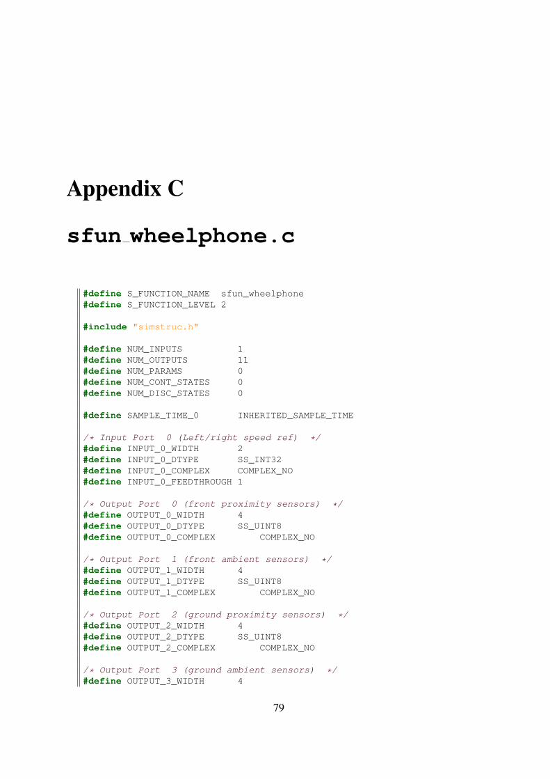
Appendix C
sfun wheelphone.c
#define S_FUNCTION_NAME sfun_wheelphone#define S_FUNCTION_LEVEL 2
#include "simstruc.h"
#define NUM_INPUTS 1#define NUM_OUTPUTS 11#define NUM_PARAMS 0#define NUM_CONT_STATES 0#define NUM_DISC_STATES 0
#define SAMPLE_TIME_0 INHERITED_SAMPLE_TIME
/* Input Port 0 (Left/right speed ref) */#define INPUT_0_WIDTH 2#define INPUT_0_DTYPE SS_INT32#define INPUT_0_COMPLEX COMPLEX_NO#define INPUT_0_FEEDTHROUGH 1
/* Output Port 0 (front proximity sensors) */#define OUTPUT_0_WIDTH 4#define OUTPUT_0_DTYPE SS_UINT8#define OUTPUT_0_COMPLEX COMPLEX_NO
/* Output Port 1 (front ambient sensors) */#define OUTPUT_1_WIDTH 4#define OUTPUT_1_DTYPE SS_UINT8#define OUTPUT_1_COMPLEX COMPLEX_NO
/* Output Port 2 (ground proximity sensors) */#define OUTPUT_2_WIDTH 4#define OUTPUT_2_DTYPE SS_UINT8#define OUTPUT_2_COMPLEX COMPLEX_NO
/* Output Port 3 (ground ambient sensors) */#define OUTPUT_3_WIDTH 4
79
80 Implementation of distributed mapping algorithms using mobile Wheelphones
#define OUTPUT_3_DTYPE SS_UINT8#define OUTPUT_3_COMPLEX COMPLEX_NO
/* Output Port 4 (battery charge [%]) */#define OUTPUT_4_WIDTH 1#define OUTPUT_4_DTYPE SS_UINT8#define OUTPUT_4_COMPLEX COMPLEX_NO
/* Output Port 5 (estimated left/right speed [mm/s]) */#define OUTPUT_5_WIDTH 2#define OUTPUT_5_DTYPE SS_INT16#define OUTPUT_5_COMPLEX COMPLEX_NO
/* Output Port 6 (odometry - x [m], y [m], yaw [rad]) */#define OUTPUT_6_WIDTH 3#define OUTPUT_6_DTYPE SS_DOUBLE#define OUTPUT_6_COMPLEX COMPLEX_NO
/* Output Port 7 (battery charging state) */#define OUTPUT_7_WIDTH 1#define OUTPUT_7_DTYPE SS_UINT8#define OUTPUT_7_COMPLEX COMPLEX_NO
/* Output Port 8 (odometry calibration flag) */#define OUTPUT_8_WIDTH 1#define OUTPUT_8_DTYPE SS_UINT8#define OUTPUT_8_COMPLEX COMPLEX_NO
/* Output Port 9 (obstacle avoidance flag) */#define OUTPUT_9_WIDTH 1#define OUTPUT_9_DTYPE SS_UINT8#define OUTPUT_9_COMPLEX COMPLEX_NO
/* Output Port 10 (cliff avoidance flag) */#define OUTPUT_10_WIDTH 1#define OUTPUT_10_DTYPE SS_UINT8#define OUTPUT_10_COMPLEX COMPLEX_NO
/*====================** S-function methods **====================*/
/* Function: mdlInitializeSizes =================================== */static void mdlInitializeSizes(SimStruct *S){ /* Number of expected parameters */
ssSetNumSFcnParams(S, NUM_PARAMS);if (ssGetNumSFcnParams(S) != ssGetSFcnParamsCount(S)) {
/* Return if number of expected != number of actual parameters */return;
}
Chapter C. sfun wheelphone.c 81
ssSetNumContStates(S, NUM_CONT_STATES);ssSetNumDiscStates(S, NUM_DISC_STATES);
if (!ssSetNumInputPorts(S, NUM_INPUTS)) return;
ssSetInputPortWidth(S, 0, INPUT_0_WIDTH);ssSetInputPortDataType(S, 0, INPUT_0_DTYPE);ssSetInputPortComplexSignal(S, 0, INPUT_0_COMPLEX);ssSetInputPortDirectFeedThrough(S, 0, INPUT_0_FEEDTHROUGH);/*direct input signal access*/ssSetInputPortRequiredContiguous(S, 0, 1);
if (!ssSetNumOutputPorts(S, NUM_OUTPUTS)) return;
ssSetOutputPortWidth(S, 0, OUTPUT_0_WIDTH);ssSetOutputPortDataType(S, 0, OUTPUT_0_DTYPE);ssSetOutputPortComplexSignal(S, 0, OUTPUT_0_COMPLEX);
ssSetOutputPortWidth(S, 1, OUTPUT_1_WIDTH);ssSetOutputPortDataType(S, 1, OUTPUT_1_DTYPE);ssSetOutputPortComplexSignal(S, 1, OUTPUT_1_COMPLEX);
ssSetOutputPortWidth(S, 2, OUTPUT_2_WIDTH);ssSetOutputPortDataType(S, 2, OUTPUT_2_DTYPE);ssSetOutputPortComplexSignal(S, 2, OUTPUT_2_COMPLEX);
ssSetOutputPortWidth(S, 3, OUTPUT_3_WIDTH);ssSetOutputPortDataType(S, 3, OUTPUT_3_DTYPE);ssSetOutputPortComplexSignal(S, 3, OUTPUT_3_COMPLEX);
ssSetOutputPortWidth(S, 4, OUTPUT_4_WIDTH);ssSetOutputPortDataType(S, 4, OUTPUT_4_DTYPE);ssSetOutputPortComplexSignal(S, 4, OUTPUT_4_COMPLEX);
ssSetOutputPortWidth(S, 5, OUTPUT_5_WIDTH);ssSetOutputPortDataType(S, 5, OUTPUT_5_DTYPE);ssSetOutputPortComplexSignal(S, 5, OUTPUT_5_COMPLEX);
ssSetOutputPortWidth(S, 6, OUTPUT_6_WIDTH);ssSetOutputPortDataType(S, 6, OUTPUT_6_DTYPE);ssSetOutputPortComplexSignal(S, 6, OUTPUT_6_COMPLEX);
ssSetOutputPortWidth(S, 7, OUTPUT_7_WIDTH);ssSetOutputPortDataType(S, 7, OUTPUT_7_DTYPE);ssSetOutputPortComplexSignal(S, 7, OUTPUT_7_COMPLEX);
ssSetOutputPortWidth(S, 8, OUTPUT_8_WIDTH);ssSetOutputPortDataType(S, 8, OUTPUT_8_DTYPE);ssSetOutputPortComplexSignal(S, 8, OUTPUT_8_COMPLEX);
ssSetOutputPortWidth(S, 9, OUTPUT_9_WIDTH);
82 Implementation of distributed mapping algorithms using mobile Wheelphones
ssSetOutputPortDataType(S, 9, OUTPUT_9_DTYPE);ssSetOutputPortComplexSignal(S, 9, OUTPUT_9_COMPLEX);
ssSetOutputPortWidth(S, 10, OUTPUT_10_WIDTH);ssSetOutputPortDataType(S, 10, OUTPUT_10_DTYPE);ssSetOutputPortComplexSignal(S, 10, OUTPUT_10_COMPLEX);
ssSetNumSampleTimes(S, 1);ssSetNumRWork(S, 0);ssSetNumIWork(S, 0);ssSetNumPWork(S, 0);ssSetNumModes(S, 0);ssSetNumNonsampledZCs(S, 0);
/* Specify the sim state compliance to be same as a built-in block */ssSetSimStateCompliance(S, USE_DEFAULT_SIM_STATE);
ssSetOptions(S, 0);}
/* Function: mdlInitializeSampleTimes ============================= */static void mdlInitializeSampleTimes(SimStruct *S){
ssSetSampleTime(S, 0, SAMPLE_TIME_0);ssSetOffsetTime(S, 0, 0.0);
// notify need to access absolute time datassSetNeedAbsoluteTime(S, 1);
}
/* Change to #undef to remove function */#undef MDL_INITIALIZE_CONDITIONS#if defined(MDL_INITIALIZE_CONDITIONS)
/* Function: mdlInitializeConditions ============================ */static void mdlInitializeConditions(SimStruct *S){}
#endif /* MDL_INITIALIZE_CONDITIONS */
/* Change to #undef to remove function */#define MDL_START#if defined(MDL_START)
/* Function: mdlStart =========================================== */static void mdlStart(SimStruct *S){}
#endif /* MDL_START */
/* Function: mdlOutputs =========================================== */static void mdlOutputs(SimStruct *S, int_T tid){
Chapter C. sfun wheelphone.c 83
}
/* Change to #undef to remove function */#undef MDL_UPDATE#if defined(MDL_UPDATE)
/* Function: mdlUpdate ========================================== */static void mdlUpdate(SimStruct *S, int_T tid){}
#endif /* MDL_UPDATE */
/* Change to #undef to remove function */#undef MDL_DERIVATIVES#if defined(MDL_DERIVATIVES)
/* Function: mdlDerivatives ===================================== */static void mdlDerivatives(SimStruct *S){}
#endif /* MDL_DERIVATIVES */
/* Function: mdlTerminate ========================================= */static void mdlTerminate(SimStruct *S){}
/*=============================** Required S-function trailer **=============================*/
#ifdef MATLAB_MEX_FILE /* Is this file being compiled as a MEX-file?
*/#include "simulink.c" /* MEX-file interface mechanism */#else#include "cg_sfun.h" /* Code generation registration function */#endif

Appendix D
sfun wheelphone.tlc
%implements "sfun_wheelphone" "C"
%include "utillib.tlc"
%assign ::includeWheelphoneSupport = 1
%function BlockTypeSetup(block, system) void%% %<LibAddToCommonIncludes("driver_wheelphone.h")>%openfile bufferextern void initWheelphone(void);extern void getWheelphoneData(time_t, uint8_t *, uint8_t *, uint8_t
*, uint8_t *,uint8_t *, int16_t *, double *,uint8_t *, uint8_t *, uint8_t *, uint8_t *);
extern void setWheelphoneSpeed(int32_t *, int32_t *);extern void terminateWheelphone(void);%closefile buffer%<LibCacheFunctionPrototype(buffer)>%<LibAddToModelSources("driver_wheelphone")>
%endfunction %% BlockTypeSetup
%function Start(block, system) OutputinitWheelphone();
%endfunction %% Start
%function Outputs(block, system) Output/* %<Type> Block: %<Name> */
%assign pu0 = LibBlockInputSignalAddr(0, "", "", 0)%assign pu1 = LibBlockInputSignalAddr(0, "", "", 1)
%assign py0 = LibBlockOutputSignalAddr(0, "", "", 0)%assign py1 = LibBlockOutputSignalAddr(1, "", "", 0)%assign py2 = LibBlockOutputSignalAddr(2, "", "", 0)%assign py3 = LibBlockOutputSignalAddr(3, "", "", 0)%assign py4 = LibBlockOutputSignalAddr(4, "", "", 0)
85
86 Implementation of distributed mapping algorithms using mobile Wheelphones
%assign py5 = LibBlockOutputSignalAddr(5, "", "", 0)%assign py6 = LibBlockOutputSignalAddr(6, "", "", 0)%assign py7 = LibBlockOutputSignalAddr(7, "", "", 0)%assign py8 = LibBlockOutputSignalAddr(8, "", "", 0)%assign py9 = LibBlockOutputSignalAddr(9, "", "", 0)%assign py10 = LibBlockOutputSignalAddr(10, "", "", 0)
getWheelphoneData(%<LibGetTaskTimeFromTID(block)>,%<py0>, %<py1>, %<py2>, %<py3>,%<py4>, %<py5>, %<py6>,%<py7>, %<py8>, %<py9>, %<py10>);
setWheelphoneSpeed(%<pu0>, %<pu1>);%endfunction %% Outputs
%function Terminate(block, system) Output
terminateWheelphone();
%endfunction %% Terminate
Appendix E
driver wheelphone.c
#include <jni.h>#include <stdlib.h>#include <math.h>
#define ENCODED_STATE_LEN 63#define MAX_BATTERY_VALUE 152#define SPEED_THR 3
#define NOT_CHARGING 0#define CHARGING 1#define CHARGED 2
#define LEFT_DIAM_COEFF 1.0#define RIGHT_DIAM_COEFF 1.0#define WHEEL_BASE 0.087
extern JavaVM *cachedJvm;extern jobject cachedActivityObj;extern jclass cachedMainActivityCls;static jmethodID sgWheelphoneGetEncodedRobotStateID;static jmethodID sgWheelphoneSetSpeedID;static jmethodID sgWheelphoneSendCmdID;
static double leftDist = 0.0;static double rightDist = 0.0;static double leftDistPrev = 0.0;static double rightDistPrev = 0.0;
static double timePrev = 0.0;
static double odometryX = 0.0;static double odometryY = 0.0;static double odometryTheta = 0.0;
void initWheelphone(void){
87
88 Implementation of distributed mapping algorithms using mobile Wheelphones
JNIEnv *pEnv;(*cachedJvm)->AttachCurrentThread(cachedJvm, &pEnv, NULL);
sgWheelphoneGetEncodedRobotStateID = (*pEnv)->GetMethodID(pEnv,cachedMainActivityCls,
"getWheelphoneEncodedState","()[B");
sgWheelphoneSetSpeedID = (*pEnv)->GetMethodID(pEnv,cachedMainActivityCls,
"setWheelphoneSpeed", "(II)V");sgWheelphoneSendCmdID = (*pEnv)->GetMethodID(pEnv,
cachedMainActivityCls,"sendWheelphoneCommands", "()V");
}
void getWheelphoneData(time_t time, uint8_t *frontProxs, uint8_t *frontAmbients,
uint8_t *groundProxs, uint8_t *groundAmbients,uint8_t *batteryCharge,int16_t *estimatedSpeed,double *odometry,uint8_t *chargeState,uint8_t *odomCalibFinish, uint8_t *obstacleAvoidanceEnabled,
uint8_t *cliffAvoidanceEnabled){
if (sgWheelphoneGetEncodedRobotStateID != NULL){
JNIEnv *pEnv;jbyteArray ret;
jbyte encodedState[ENCODED_STATE_LEN];
int16_t leftMeasuredSpeed, rightMeasuredSpeed;uint8_t batteryRaw;float batteryVoltage;uint8_t flagRobotToPhone;
time_t totalTime;
double deltaDist;
(*cachedJvm)->AttachCurrentThread(cachedJvm, &pEnv, NULL);
ret = (jintArray)(*pEnv)->CallObjectMethod(pEnv,cachedActivityObj, sgWheelphoneGetEncodedRobotStateID);
if ((*pEnv)->ExceptionCheck(pEnv))return; /* Exception during execution of
sgWheelphoneGetEncodedRobotStateID */
(*pEnv)->GetByteArrayRegion(pEnv, ret, 0, ENCODED_STATE_LEN, (jbyte *)encodedState);
Chapter E. driver wheelphone.c 89
if ((*pEnv)->ExceptionCheck(pEnv)){
(*pEnv)->DeleteLocalRef(pEnv, ret);return; /* ArrayIndexOutOfBoundsException */
}
frontProxs[0] = (uint8_t)encodedState[1];frontProxs[1] = (uint8_t)encodedState[2];frontProxs[2] = (uint8_t)encodedState[3];frontProxs[3] = (uint8_t)encodedState[4];
frontAmbients[0] = (uint8_t)encodedState[5];frontAmbients[1] = (uint8_t)encodedState[6];frontAmbients[2] = (uint8_t)encodedState[7];frontAmbients[3] = (uint8_t)encodedState[8];
groundProxs[0] = (uint8_t)encodedState[9];groundProxs[1] = (uint8_t)encodedState[10];groundProxs[2] = (uint8_t)encodedState[11];groundProxs[3] = (uint8_t)encodedState[12];
groundAmbients[0] = (uint8_t)encodedState[13];groundAmbients[1] = (uint8_t)encodedState[14];groundAmbients[2] = (uint8_t)encodedState[15];groundAmbients[3] = (uint8_t)encodedState[16];
// battery level (from 0 to maxBatteryValue=152)batteryRaw = (uint8_t)encodedState[17];
// battery voltage (from 3.5 to 4.2 volts)// 915 is the ADC out at 4.2 volts// 763 is the ADC out at 3.5 volts// the "battery" variable actually contains the "sampled value -
763"batteryVoltage = 4.2*(float)((batteryRaw + 763)/915.0);
// remaining battery charge (from 0% to 100%)
*batteryCharge = 100*batteryRaw/MAX_BATTERY_VALUE;
flagRobotToPhone = (uint8_t)encodedState[18];
// estimated speed (from back EMF) in [mm/s]leftMeasuredSpeed = (uint8_t)encodedState[19] + 256*(uint8_t)
encodedState[20];rightMeasuredSpeed = (uint8_t)encodedState[21] + 256*(uint8_t)
encodedState[22];
if (abs(leftMeasuredSpeed) < SPEED_THR) {leftMeasuredSpeed = 0;
}if (abs(rightMeasuredSpeed) < SPEED_THR) {
90 Implementation of distributed mapping algorithms using mobile Wheelphones
rightMeasuredSpeed = 0;}
estimatedSpeed[0] = leftMeasuredSpeed;estimatedSpeed[1] = rightMeasuredSpeed;
// estimated travelled distance [m]leftDistPrev = leftDist;rightDistPrev = rightDist;totalTime = time - timePrev;leftDist += (leftMeasuredSpeed/1000.0 * totalTime) *
LEFT_DIAM_COEFF;rightDist += (rightMeasuredSpeed/1000.0 * totalTime) *
RIGHT_DIAM_COEFF;deltaDist = ((rightDist - rightDistPrev) + (leftDist -
leftDistPrev)) / 2.0;
// odometry [m], [rad]odometryX += cos(odometryTheta) * deltaDist;odometryY += sin(odometryTheta) * deltaDist;odometryTheta = ((rightDist - leftDist) / WHEEL_BASE) / 1000.0;
odometry[0] = odometryX;odometry[1] = odometryY;odometry[2] = odometryTheta;
// battery charging stateif ((flagRobotToPhone & 0x20) == 0x20) {
if ((flagRobotToPhone & 0x40) == 0x40) {
*chargeState = CHARGED;} else {
*chargeState = CHARGING;}
} else {
*chargeState = NOT_CHARGING;}
// odometry calibration flagif ((flagRobotToPhone & 0x80) == 0x80) {
*odomCalibFinish = 1;} else {
*odomCalibFinish = 0;}
// obstacle avoidance flagif ((flagRobotToPhone & 0x01) == 0x01) {
*obstacleAvoidanceEnabled = 1;} else {
*obstacleAvoidanceEnabled = 0;}
Chapter E. driver wheelphone.c 91
// cliff avoidance flagif ((flagRobotToPhone & 0x02) == 0x02) {
*cliffAvoidanceEnabled = 1;} else {
*cliffAvoidanceEnabled = 0;}
(*pEnv)->DeleteLocalRef(pEnv, ret);}
}
void setWheelphoneSpeed(int32_t *lSpeed, int32_t *rSpeed){
if ( (sgWheelphoneSetSpeedID != NULL) && (sgWheelphoneSendCmdID !=NULL) )
{JNIEnv *pEnv;jint jlSpeed = (jint)*lSpeed;jint jrSpeed = (jint)*rSpeed;
(*cachedJvm)->AttachCurrentThread(cachedJvm, &pEnv, NULL);
(*pEnv)->CallVoidMethod(pEnv, cachedActivityObj,sgWheelphoneSetSpeedID,
jlSpeed, jrSpeed);if ((*pEnv)->ExceptionCheck(pEnv))
return; /* Exception during execution ofsgWheelphoneSetSpeedID */
(*pEnv)->CallVoidMethod(pEnv, cachedActivityObj,sgWheelphoneSendCmdID);
if ((*pEnv)->ExceptionCheck(pEnv))return; /* Exception during execution of
sgWheelphoneSendCmdID */}
}
void terminateWheelphone(void){}

Appendix F
wheelphonelib.tlc
%function FcnGenWheelphoneLib() void%assign tgtData = FEVAL("get_param", CompiledModel.Name, "
TargetExtensionData")%assign packageName = "%<tgtData.packagename>.%<CompiledModel.Name>"%openfile wheelphoneLibFile = "WheelphoneRobot.java"%selectfile wheelphoneLibFile
package %<packageName>;
import android.content.Context;import android.content.Intent;import android.os.Handler;import android.os.Message;
public class WheelphoneRobot {
// USB communicationprivate final static int packetLengthRecv = 63; // receiving
packet length (this the maximum packet length, actually only 23bytes are used)
private final static int packetLengthSend = 63; // sendingpacket legnth (this the maximum packet length, actually only 3bytes are used)
private final static int USBAccessoryWhat = 0; // type ofmessage received
private static final int APP_CONNECT = (int) 0xFE;private static final int APP_DISCONNECT = (int) 0xFF;private static final int UPDATE_STATE = 4;private boolean deviceAttached = false;private boolean isConnected = false; // flag
indicating if the robot is connected (and exchanging packets) withthe phone
private int firmwareVersion = 0;private USBAccessoryManager accessoryManager;
// Packet received from PIC with encoded robot stateprivate byte[] encodedRobotState = new byte[packetLengthRecv];
93
94 Implementation of distributed mapping algorithms using mobile Wheelphones
// Robot control (phone => robot)private int lSpeed = 0, rSpeed = 0;private static final int MIN_SPEED_RAW = -127;private static final int MAX_SPEED_RAW = 127;private static final int MIN_SPEED_REAL = -350;private static final int MAX_SPEED_REAL = 350;private static final double MM_S_TO_BYTE = 2.8; // scale
the speed given in mm/s to a byte sent to the microcontrollerprivate byte flagPhoneToRobot = 1; // bit 0 => controller On/Off
// bit 1 => soft accelerationOn/Off
// bit 2 => obstacleavoidance On/Off
// bit 3 => cliff avoidanceOn/Off
// others bits not used
// Othersprivate Context context;private Intent activityIntent;
/** Interface that should be implemented by classes that would like to
be notified by when
* the WheelphoneRobot state is updated.
*/public interface WheelphoneRobotListener {
void onWheelphoneUpdate();}
private WheelphoneRobotListener mEventListener;
// Handler for receiving messages from the USB Manager threadprivate Handler handler = new Handler() {
Overridepublic void handleMessage(Message msg) {
byte[] commandPacket1 = new byte[2];byte[] commandPacket2 = new byte[packetLengthSend];
switch (msg.what) {
case USBAccessoryWhat:
switch (((USBAccessoryManagerMessage) msg.obj).type){
case CONNECTED:break;
Chapter F. wheelphonelib.tlc 95
case DISCONNECTED:isConnected = false;
//Notify listener of a disconnectionif(mEventListener!=null) {
mEventListener.onWheelphoneUpdate();}break;
case READY:
String version = ((USBAccessoryManagerMessage) msg.obj).accessory.getVersion();
firmwareVersion = getFirmwareVersion(version);
switch (firmwareVersion) {case 1:
deviceAttached = true;break;
case 2:case 3:
// send connection req to WheelphonePIC24F
commandPacket1[0] = (byte)APP_CONNECT;
commandPacket1[1] = 0;accessoryManager.write(commandPacket1
);deviceAttached = true;
// enable control to get new packetwith Wheelphone state
commandPacket2[0] = (byte)UPDATE_STATE;
commandPacket2[1] = (byte) 0;commandPacket2[2] = (byte) 0;commandPacket2[3] = flagPhoneToRobot;accessoryManager.write(commandPacket2
);break;
default:break;
}
isConnected = true;break;
96 Implementation of distributed mapping algorithms using mobile Wheelphones
case READ:if (accessoryManager.isConnected() == false)
{return;
}
while (true) {if (accessoryManager.available() <
packetLengthRecv) {break;
}
accessoryManager.read(encodedRobotState);
switch(encodedRobotState[0]) {case UPDATE_STATE:
//Notify listener of an updateif(mEventListener!=null) {
mEventListener.onWheelphoneUpdate();
}break;
}
}break;
case ERROR:break;
default:break;
}}
}};
/*** \brief Class constructor
* \param a pass the main activity instance (this)
* \return WheelphoneRobot instance
*/public WheelphoneRobot(Context c, Intent i) {
context = c;activityIntent = i;mEventListener = null;
}
public void createUSBCommunication() {accessoryManager = new USBAccessoryManager(handler,
USBAccessoryWhat);
Chapter F. wheelphonelib.tlc 97
}
/*** \brief To be inserted into the "onResume" function of the main
activity class.
* \return none
*/public void openUSBCommunication() {
accessoryManager.enable(context, activityIntent);}
/*** \brief To be inserted into the "onPause" function of the main
activity class.
* \return none
*/public void closeUSBCommunication() {
accessoryManager.disable(context);
switch (firmwareVersion) {case 2:case 3:
byte[] commandPacket = new byte[2];commandPacket[0] = (byte) APP_DISCONNECT;commandPacket[1] = 0;accessoryManager.write(commandPacket);break;
}try {
while (accessoryManager.isClosed() == false) {Thread.sleep(2000);
}} catch (InterruptedException e) {
e.printStackTrace();}isConnected = false;
}
/*** \brief Set listener to be notified by when the WheelphoneRobot
state is updated. .
* \return none
*/public void setWheelphoneRobotListener(WheelphoneRobotListener
eventListener) {mEventListener = eventListener;
}
/**
98 Implementation of distributed mapping algorithms using mobile Wheelphones
* \brief Remove listener to be notified by when the WheelphoneRobotstate is updated. .
* \return none
*/public void removeWheelphoneRobotListener() {
mEventListener = null;}
/*** \brief Send the next packet to the robot containing the last left
and right speeds and flag data.
* Use the speed references set with the setSpeed methods.
* \return none
*/public void sendCommandsToRobot() {
if (accessoryManager.isConnected() == false) {return;
}byte[] commandPacket = new byte[packetLengthSend];commandPacket[0] = (byte) UPDATE_STATE;commandPacket[1] = (byte) lSpeed; // left speed refcommandPacket[2] = (byte) rSpeed; // right speed refcommandPacket[3] = flagPhoneToRobot; // (control enable)accessoryManager.write(commandPacket);
}
/*** \brief Turn Wheelphone motors off.
* \return none
*/public void turnMotorsOff() {
if (accessoryManager.isConnected() == false) {return;
}byte[] commandPacket = new byte[packetLengthSend];commandPacket[0] = (byte) UPDATE_STATE;commandPacket[1] = 0; // left speed refcommandPacket[2] = 0; // right speed refcommandPacket[3] = flagPhoneToRobot; // (control enable)accessoryManager.write(commandPacket);
}
/*** \brief Retrieve firmware version from USB version
* \param string with USB version
* \return firmware version installed on Wheelphone PIC24F
*/private int getFirmwareVersion(String version) {
String major = "0";int positionOfDot;
Chapter F. wheelphonelib.tlc 99
positionOfDot = version.indexOf(’.’);if (positionOfDot != -1) {
major = version.substring(0, positionOfDot);}
return new Integer(major).intValue();}
/*** \brief Return version of the firmware running on the robot. This
is useful to know whether an update is available or not.
* \return firmware version
*/public int getFirmwareVersion() {
return firmwareVersion;}
/*** \brief Return the encoded robot state (i.e. packet received from
onboard PIC)
* \return encoded robot state
*/public byte[] getEncodedRobotState() {
return encodedRobotState;}
/*** \brief Indicate whether the robot is connected (and exchanging
packets) with the phone or not.
* \return true (if robot connected), false otherwise
*/public boolean isRobotConnected() {
return isConnected;}
/*** \brief Set the new left and right speeds for the robot. The new
data
* will be actually sent to the robot when "sendCommandsToRobot" is
* called the next time within the timer communication task (50 mscadence). This means that the robot speed will be updated
* after at most 50 ms (if the task isn’t delayed by the system).
* \param l left speed given in mm/s
* \param r right speed given in mm/s
* \return none
*/public void setSpeed(int l, int r) { // speed given in mm/s
if(l < MIN_SPEED_REAL) {l = MIN_SPEED_REAL;
}if(l > MAX_SPEED_REAL) {
100 Implementation of distributed mapping algorithms using mobile Wheelphones
l = MAX_SPEED_REAL;}if(r < MIN_SPEED_REAL) {
r = MIN_SPEED_REAL;}if(r > MAX_SPEED_REAL) {
r = MAX_SPEED_REAL;}lSpeed = (int) (l/MM_S_TO_BYTE);rSpeed = (int) (r/MM_S_TO_BYTE);
}
/*** \brief Set the new left and right speeds for the robot. For more
details refer to "setSpeed".
* \param l left speed (range is from -127 to 127)
* \param r right speed (range is from -127 to 127)
* \return none
*/
public void setRawSpeed(int l, int r) {if(l < MIN_SPEED_RAW) {
l = MIN_SPEED_RAW;}if(l > MAX_SPEED_RAW) {
l = MAX_SPEED_RAW;}if(r < MIN_SPEED_RAW) {
r = MIN_SPEED_RAW;}if(r > MAX_SPEED_RAW) {
r = MAX_SPEED_RAW;}lSpeed = l;rSpeed = r;
}}
%closefile wheelphoneLibFile%endfunction
Bibliography
[1] Brian Yamauchi. A Frontier-Based Approach for Autonomous Exploration. Proceedings ofthe 1997 IEEE International Symposium on Computational Intelligence in Robotics and Au-tomation, Monterey, CA, July 1997, pp. 146-151
[2] G. Dudek, M. Jenkin, E. Milios and D. Wilkes. Robotic exploration as graph construction..PIEEE Transactions on Robotics and Automation, 7:6, pp. 859-865, 1991.
[3] Brian Yamauchi. Frontier-Based Exploration Using Multiple Robots. Proceedings of the Sec-ond International Conference on Autonomous Agents (Agents ’98), Minneapolis, MN, May1998, pp. 47-53
[4] B. Yamauchi, ”Decentralized coordination for multirobot exploration” Robotics and Au-tonomous Systems, vol. 29, no. 2-3, pp. 111-118, 1999.
[5] R. Simmons, D. Apfelbaum, W. Burgard, D. Fox, M. Moors, S. Thrun, and H. Younes,”Coordination for multi-robot exploration and mapping” in Proceedings of the NationalConference on Artificial Intelligence, 2000, pp. 852-858.
[6] W. Burgard, M. Moors, C. Stachniss, and F. Schneider, ”Coordinated multi- robot explo-ration” IEEE Transactions on Robotics, vol. 21, no. 3, pp. 376- 386, 2005.
[7] Ling Wu, Miguel Angel Garcia, Domenec Puig and Albert Sole, ”Voronoi-Based SpacePartitioning for Coordinated Multi-Robot Exploration” Journal Of Physical Agents, vol. 1,no. 1, 2007
[8] Keith Kotay, Ron Peterson, and Daniela Rus, ”Experiments with Robots and Sensor Net-works for Mapping and Navigation Field and Service Robotics Results of the 5th Interna-tional Conference. 2006
[9] L. Ljung, editor. ”System Identification (2Nd Ed.): Theory for the User”. Prentice Hall PTR,Upper Saddle River, NJ, USA, 1999.
[10] T. Soderstrom and P. Storica, editors. System Identification”. Prentice-Hall, Inc., UpperSaddle River, NJ, USA, 1988.
[11] G. Pillonetto, A. Chiuso, and G. De Nicolao. ”Prediction error identification of linear sys-tems: A nonparametric Gaussian regression approach”. Automatica, 47(2):291 305, 2011.
101
102 Implementation of distributed mapping algorithms using mobile Wheelphones
[12] T. Poggio and F. Girosi. ”Networks for approximation and learning”. In Proceedings of theIEEE, volume 78, pages 14811497, 1990.
[13] S. Smale and D.X. Zhou. ”Online learning with Markov sampling”. Analysis and Applica-tions, 07(01):87113, 2009.
[14] Y. Xu, J. Choi, S. Dass, and T. Maiti. ”Sequential Bayesian prediction and adaptive sam-pling algorithms for mobile sensor networks”. IEEE Transactions on Automatic Control,57(8):20782084, 2012.
[15] Y. Xu, J. Choi, and S. Oh. ”Mobile sensor network navigation using Gaussian processeswith truncated observations”. IEEE Transactions on Robotics, 27(6):11181131, 2011.
[16] Y. Xu, J. Choi, S. Dass, and T. Maiti. ”Efficient Bayesian spatial prediction with mobile sen-sor networks using Gaussian Markov random fields”. Automatica, 49(12):35203530, 2013.
[17] Nikolay A Atanasov, Jerome Le Ny, and George J Pappas. ”Distributed algorithms forstochastic source seeking with mobile robot networks”. Journal of Dynamic Systems, Mea-surement, and Control, 137(3):031004, 2015.
[18] J. Choi, J. Lee, and S. Oh. ”Swarm intelligence for achieving the global maximum us-ing spatio-temporal Gaussian processes”. In American Control Conference, 2008, pages135140. IEEE, 2008.
[19] M. Todescato, A. Carron, R. Carli, G. Pillonetto, L. Schenato. ”Multi-Robots GaussianEstimation and Coverage Control: from Server-based to Distributed Architecture”. Auto-matica, 20XX
[20] A. N. Tikhonov and V. Y. Arsenin, ”Solution of Ill-posed Problems”. Wiston, 1977.
[21] F. Girosi, M. Jones, and T. Poggio, Regularization theory and neural networks architecture,Neural Computation, vol. 7, pp. 219269, 1995.
[22] K.S.Arun,T.S.Huang,S.D.Blostein, Least-Square Fitting of two 3D Point Set Neural Com-putation