Impact of Liming Ratio on Lime Mud Settling and Filterability in the

Impact of Liming Ratio on Lime Mud Settling and

Filterability in the Kraft Recovery Process

by

Fariba Azgomi

A thesis submitted in conformity with the requirements

for the degree of Doctor of Philosophy

Graduate Department of Chemical Engineering and Applied Chemistry

University of Toronto

© Copyright by Fariba Azgomi 2014

ii

Impact of Liming Ratio on Lime Mud Settling and Filterability in

the Kraft Recovery Process

Fariba Azgomi

Degree of Doctor of Philosophy

Graduate Department of Chemical Engineering and Applied Chemistry

University of Toronto

2014

Abstract

In kraft pulp mills, lime is used to convert sodium carbonate to sodium hydroxide (Ca(OH)2).

The causticizing reaction precipitates lime mud which is washed, dewatered, and calcined in a

lime kiln to generate lime for reuse. Clean, dry, and more stable lime mud helps reducing the

energy usage of the kiln, improving burner flame stability, minimizing ring formation, and

alleviating emissions of reduced sulphur gases from the kiln stack.

The dewatering efficiency of lime mud is greatly affected by the mud and liquor properties, and

the equipment design and operation. The properties of the mud vary continuously due to changes

in the liquor strength, lime quality and dosage, which is known as the “liming ratio”. Many

studies have been carried out to relate lime mud properties to dewatering and filtration

behaviours, the mechanisms by which lime mud becomes difficult to settle and filter are not well

understood.

A systematic study was therefore conducted to examine the effect of the liming ratio on the

settling rate and filterability of lime mud. The results show that the mud settling rate and

filterability decreased with an increase in liming ratio. The effect was more noticeable as the

liming ratio exceeded a critical level leading to an overliming condition. The results also show

that the particle size of the resulting lime mud did not appreciably change with liming ratio.

Therefore, the decrease in settling rate and filterability cannot be attributed to the smaller particle

iii

size of Ca(OH)2 compared to that of lime mud as commonly believed. Rather, it was caused by a

change in zeta potential of Ca(OH)2-containing mud particles.

This study also shows that the zeta potential of the mud slurry increases proportionally to the free

lime content in the lime mud. This suggests that the zeta potential can be used to indicate the

extent of overliming in the causticizing plant. The correlation between zeta potential and free

lime content can be used to develop an on-line overliming monitoring system to help regulate the

amount of lime addition to the system to achieve optimum operating conditions for the mud

settling and filtering equipment.

iv

Acknowledgements

I wish to express my sincerest appreciation and utmost gratitude to my supervisor, Professor

Honghi Tran for his excellent supervision, continuous support, and valuable technical assistance

and discussion. I particularly appreciate the relationship that has been established between us

along the course of my study, and that will enrich my memories all my life.

I would also like to express my heartfelt thanks to my co-supervisor, Professor Ramin Farnood

where his professional guidance, and contribution proved priceless to the work presented in this

thesis.

Gratitude and recognition go to my supervisory committee, Professor Donald Kirk, and Professor

Edgar Acosta, for their advice, feedback and comments. In addition, I would like to thank

Professor John Cameron for acting as the external examiner in my final defense.

Thanks must also go to the Professor Tran group members (old and new) for providing support

and encouragement during the smooth and rough periods of my work. They made my time at U

of T worthwhile and I learned a lot from all of them, especially to Ms. Sue Mao and Dr. Daniel

Saturnino for valuable suggestions and fruitful discussion.

I would like to express my appreciation to the faculty and staff of the Chemical Engineering and

Applied Chemistry Department at the University of Toronto for fostering a pleasant

environment. My special gratitude goes out to Ms. Pauline Martini and Ms. Anna Ho.

I would also like to acknowledge financial support of members of research consortium on

Increasing Energy and Chemical Recovery in the Kraft Pulping Process.

My parents, Farzaneh and Azim, have been a source of inspiration all throughout my life and the

true reason behind my achievements. They taught me the importance of a strong education and

have always encouraged me to pursue my education to the highest levels. For that, I am eternally

grateful.

Furthermore, many thanks go to my sisters, Foroozan, and Foroozesh and her family, for always

supporting and encouraging me throughout my education.

v

I cordially thank my sweet little son, Arad, who teaches me to enjoy every moment of life and to

put everything in perspective.

Last, but not least, I could never express adequately written words for the thanks I owe to my

husband, Sina. He has had to make many sacrifices during the past five years in order to support

me in the work I have been doing. I am certain that had it not been for his love, continuous

motivation and unfailing support, I would never have accomplished my goals. This dissertation is

dedicated to my parents, my dear husband and my son.

vi

Table of Contents

1 Introduction .......................................................................................................................... 1

1.1 General Background ......................................................................................................... 1

1.2 Lime Mud Dewatering ..................................................................................................... 3

1.3 Parameters Affecting Lime Mud Filtration and Dewatering Efficiency .......................... 5

1.4 Objective .......................................................................................................................... 7

1.5 Structure of Thesis ........................................................................................................... 7

2 Literature Review ................................................................................................................. 8

2.1 Settling Theory ................................................................................................................. 8

2.1.1 Mathematical Model for Batch Settling .................................................................. 10

2.1.1.1 Kynch Theory .................................................................................................. 10

2.1.1.2 Theoretical Batch Settling Curve .................................................................... 12

2.2 Filtration Theory ............................................................................................................ 14

2.3 Forces Involved in Aggregation/Dispersion .................................................................. 17

2.3.1 Van der Waals Forces ............................................................................................. 17

2.3.2 Electrostatic Forces ................................................................................................. 18

2.3.2.1 Development of Electrical Double Layer ........................................................ 18

2.3.3 Zeta potential (ζ) ..................................................................................................... 20

2.4 Correlation Between Sedimentation Volume and Colloid Stability .............................. 22

2.5 Influence of Particle Properties on Lime Mud Dewatering ........................................... 23

2.5.1 The Calcite/Water System ...................................................................................... 24

2.5.2 Zeta Potential of Calcite .......................................................................................... 24

2.5.3 Influence of Inorganic Ions on the Surface Charge of Calcite ................................ 25

2.6 Lime Mud Settling and Filterability - Previous Studies ................................................. 26

2.6.1 Definitions ............................................................................................................... 26

2.6.1.1 Causticizing Efficiency .................................................................................... 26

2.6.1.2 Total Titratable Alkali and Active Alkali ........................................................ 26

2.6.1.3 Sulfidity ........................................................................................................... 27

2.6.1.4 Liming Ratio .................................................................................................... 27

2.6.2 Physical Properties of Lime and Lime Mud ........................................................... 28

2.6.2.1 Lime Quality .................................................................................................... 28

2.6.2.2 Chemical Composition of Lime Mud .............................................................. 30

2.6.2.3 Lime Dosage (Liming Ratio) ........................................................................... 31

2.6.3 Influence of Liqour Properties on Lime Mud Dewatering ..................................... 32

2.6.4 Influence of Operation Variables on Lime Mud Dewatering ................................. 33

2.6.5 Influence of Equipment Design and Operation on Lime Mud Dewatering ............ 34

2.7 Summary ........................................................................................................................ 36

3 Experimental Techniques .................................................................................................. 37

3.1 Slaking and Causticizing Reactions ............................................................................... 37

3.2 Settling ........................................................................................................................... 38

3.2.1 Five-Minute Settling Test ....................................................................................... 39

3.3 Filterability ..................................................................................................................... 40

3.3.1 Original Set-up ........................................................................................................ 40

3.3.2 Modified Set-up ...................................................................................................... 41

3.4 Titration .......................................................................................................................... 42

3.5 Particle Size Distribution (PSD) .................................................................................... 42

3.6 Surface Area of Particle ................................................................................................. 43

vii

3.7 Zeta Potential .................................................................................................................. 43

3.8 Thermal Gravimetric Analysis ....................................................................................... 44

3.9 Scanning Electron Microscopy ...................................................................................... 44

3.10 Atomic Absorption Spectroscopy (AAS) ................................................................... 45

3.11 X-ray Florescence Spectroscopy (XRF) ..................................................................... 45

3.12 X-Ray Diffraction Analysis (XRD) ............................................................................ 45

3.13 OLI, Advanced Simulation Software ......................................................................... 45

4 Experimental Results and Discussion ............................................................................... 47

4.1 Reburned Lime Characteristics ...................................................................................... 48

4.2 Lime Mud Settling ......................................................................................................... 50

4.2.1 Liming Ratio ........................................................................................................... 50

4.2.2 Effect of Solids Content .......................................................................................... 57

4.2.3 Lime Type ............................................................................................................... 61

4.3 Lime Mud Filterability ................................................................................................... 64

4.3.1 Liming Ratio ........................................................................................................... 64

4.3.2 Effect of Solids Content .......................................................................................... 65

4.3.3 Lime Type ............................................................................................................... 70

4.4 Causticizing Efficiency .................................................................................................. 73

4.5 Particle Size Distribution and Morphology .................................................................... 74

4.5.1 Effect of Liming Ratio ............................................................................................ 74

4.5.2 Effect of Lime Type ................................................................................................ 79

4.6 Evolution of Particle Size Distribution during Slaking and Causticizing Reactions ..... 81

4.6.1 Comparing Physical Properties of CaCO3 and Ca(OH)2 Particles ......................... 82

4.6.2 Taking Samples During Slaking and Causticizing Reactions ................................. 85

4.7 Zeta Potential .................................................................................................................. 88

5 Relationship between Zeta Potential and Kozeny Coefficient ....................................... 98

5.1 Results and Discussion ................................................................................................... 98

5.1.1 General Approach ................................................................................................... 98

5.1.2 Kozeny Coefficient ................................................................................................. 99

5.2 Parametric Study: Effect of Particle Size and Concentration ...................................... 103

5.2.1 Effect of Particle Size on Settling Rate of CaCO3 Particles ................................. 103

5.2.2 Effect of Initial Solids Content on Settling Rate of CaCO3 Particles ................... 105

6 Practical Implications ...................................................................................................... 107

7 Conclusions and Recommendations ............................................................................... 108

7.1 Conclusions .................................................................................................................. 108

7.2 Recommendations ........................................................................................................ 109

8 Reference ........................................................................................................................... 111

Appendix A: Type I and II Settling ........................................................................................ 120

Appendix B: Selecting Graduated Cylinder Height and Diameter ..................................... 122

Appendix C: Atomic Absorption Spectroscopy (AAS) ......................................................... 125

Appendix D: Settling Results .................................................................................................. 127

Appendix E: Filterability Results ........................................................................................... 129

Appendix F: Particle Size Distribution Results ..................................................................... 130

Appendix G: Liquid Density and Viscosity Measurements ................................................. 132

Appendix H: Effect of Electrolyte Concentration on Settling .............................................. 134

Appendix I: Zeta potential Measurements of Pure Ca(OH)2 and CaCO3 .......................... 136

viii

List of Tables

Table 4-1: Physical and Chemical Characteristics of Reburned Limes ........................................ 50

Table 4-2: Calculation of Cake Specific Resistance and Apparent Medium Resistance Values of

lime muds at Different Liming Ratio at 65 Kilopascal Vacuum .................................................. 69

Table 4-3: Calculation of Specific Cake Resistance and Apparent Medium Resistance Values of

Different Lime Types at 65 Kilopascal Vacuum .......................................................................... 73

Table 4-4: Summary of Parameters Related to Size Distribution ................................................. 76

Table 5-1: Summary of Zeta Potential of Particles and Estimated Kozeny Coefficients ........... 101

ix

List of Figures

Figure 1-1: Schematic of the Kraft Recovery Process [3] .............................................................. 2

Figure 1-2: Schematic Diagram of Causticizing Plant [4] .............................................................. 3

Figure 1-3: Rotary Vacuum Precoat Drum Filter, Courtesy of Dorr-Oliver Eimco [5] ................. 4

Figure 1-4: View of Lime Mud Discharging from Lime Mud Rotary Vacuum Precoat Drum

Filter, Courtesy of Dorr-Oliver Eimco [5] ...................................................................................... 4

Figure 1-5: Estimated Heat Consumption of Lime Kiln per Ton of Lime Mud as a Function of

Dry Solids Content in Lime Mud Feed to the Kiln [6] ................................................................... 5

Figure 2-1: Flux Variations during Batch Sedimentation ............................................................. 11

Figure 2-2: Solids Concentration Characteristics during Settling ................................................ 12

Figure 2-3: Gouy-Chapman Model with Stern Modifications [44] .............................................. 19

Figure 2-4: Interaction Energy Profile .......................................................................................... 20

Figure 2-5: Schematic of Oliver-type Rotary Vacuum Drum Filter ............................................. 35

Figure 3-1: Schematic of the Slaking and Causticizing Vessel .................................................... 37

Figure 3-2: Settling Test Set-up .................................................................................................... 39

Figure 3-3: Bench Scale Dewatering Equipment Set-up ............................................................. 40

Figure 3-4: Filterability Test Set-up ............................................................................................. 42

Figure 3-5: Zeta Plus Optics Apparatus ........................................................................................ 44

Figure 4-1: SEM of Reburned Limes, a) Mill A, b) Mill B, c) Mill C, d) Mill D, and e) Pure CaO

....................................................................................................................................................... 49

Figure 4-2: Appearance of Mud Settling in the Cylinder (LR= 0.6, 120 g/L Na2O TTA, and 90

minutes reaction) ........................................................................................................................... 51

Figure 4-3: Effect of Liming Ratio on Settling Curve (120 g/L Na2O TTA, and 90 minutes

reaction), Pure CaO ....................................................................................................................... 52

Figure 4-4: Settling Velocity as a Function of Lime Dosage (120 g/L Na2O TTA, and 90 minutes

reaction), Pure CaO ....................................................................................................................... 53

Figure 4-5: Effect of Liming Ratio on Settling Curve (120 g/L Na2O TTA, and 90 minutes

reaction), R-Lime “B” ................................................................................................................... 54

Figure 4-6: Comparing Settling Velocity of Pure Lime and R-Lime “B” as a Function of Liming

Ratio (120 g/L Na2O TTA, and 90 minutes reaction) ................................................................... 55

Figure 4-7: The Batch Flux Curve as a Function of Lime Ratio (120 g/L Na2O TTA, and 90

minutes reaction), R-Lime “B” ..................................................................................................... 56

Figure 4-8: Relationship between Liming Ratio and Final Interface Height shown in Figure 4-5

....................................................................................................................................................... 57

Figure 4-9: Effect of Solids Content on Settling Curve (R-Lime “B”, [CaO]/ [Na2CO3] =1, 120

g/L Na2O TTA, and 90 minutes reaction) ..................................................................................... 58

Figure 4-10: Effect of Solids Concentration on Settling Velocity (R-Lime “B”, [CaO]/ [Na2CO3]

=1, 120 g/L Na2O TTA, and 90 minutes reaction) ....................................................................... 59

Figure 4-11: Effect of Liming Ratio on Settling Curve of Mud Produced from Mill B Reburned

Lime at a Constant Slurry Concentration of 6 wt. % (120 g/L Na2O TTA, and 90 minutes

reaction) ........................................................................................................................................ 60

Figure 4-12: Effect of Liming Ratio on Settling Curve of Mud Produced from Mill B Lime at a

Constant Slurry Concentration of 20 wt. % (120 g/L Na2O TTA, and 90 minutes reaction) ....... 61

Figure 4-13: Effect of Lime Type on Settling Curve ([CaO]/ [Na2CO3] =1, 120 g/L Na2O TTA,

and 90 minutes reaction) ............................................................................................................... 62

Figure 4-14: Relationship Between Lime Types and Final Interface Height Shown in Figure 4-13

....................................................................................................................................................... 62

x

Figure 4-15: Effect of Type of Lime on 5-minute Rate as Function of Liming Ratio (120 g/L

Na2O TTA, and 90 minutes reaction) ........................................................................................... 63

Figure 4-16: t/V vs. V Plots as Function of Liming Ratio (120 g/L Na2O TTA, 90 minutes

reaction, and 14 KPa Vacuum), R-Lime “B” using Filterability Set-up as Shown in Figure 3-3 65

Figure 4-17: Raw Data - Effect of Liming Ratios on Filtration at a Constant Solid Concentration

of 20 wt. %, (Pure CaO, 120 g/L Na2O TTA, and 90 minutes reaction, 65 KPa Vacuum) using

Filterability Set-up Shown in Figure 3-4 ...................................................................................... 67

Figure 4-18: Corrected Data - Effect of Liming Ratios on Filtration at a Constant Solid

Concentration of 20 wt. %, (Pure CaO, 120 g/L Na2O TTA, and 90 minutes reaction, 65 KPa

Vacuum) using Filterability Set-up Shown in Figure 3-4 ............................................................. 67

Figure 4-19: Relationship between Liming Ratio and Filtration Rate Shown in Figure 4-18

(Solids Content of 20 wt. %) ......................................................................................................... 68

Figure 4-20: t/V vs. V Plots at Different Liming Ratio (Pure CaO, 120 g/L Na2O TTA, and 90

minutes reaction, 65 KPa Vacuum, Constant Solids Concentration of 20 wt. %,) using

Filterability Data Shown in Figure 4-18 ....................................................................................... 69

Figure 4-21: Raw Data - Effect of Type of Lime on Filtration Curve ([CaO]/ [Na2CO3] =1, 20

wt. % solids, 120 g/L Na2O TTA, and 90 minutes reaction) using Filterability Set-up Shown in

Figure 3-4 ...................................................................................................................................... 71

Figure 4-22: Corrected Data - Effect of Type of Lime on Filtration Curve ([CaO]/ [Na2CO3] =1,

20 wt. % solids, 120 g/L Na2O TTA, and 90 minutes reaction) using Filterability Set-up Shown

in Figure 3-4 .................................................................................................................................. 71

Figure 4-23: Effect of Lime Type on Cake Moisture Content ([CaO]/ [Na2CO3] =1, 20 wt. %

solids, 120 g/L Na2O TTA, and 90 minutes reaction) .................................................................. 72

Figure 4-24: Effect of Liming Ratio on CE as a Function of Lime Type (120 g/L Na2O TTA, and

90 minutes reaction) ...................................................................................................................... 74

Figure 4-25: Effect of Liming Ratio on Particle Size Distribution (120 g/L Na2O TTA, and 90

minutes reaction), R-Lime “B” ..................................................................................................... 75

Figure 4-26: Relationship between Liming Ratio and 85th

Percentile Diameter shown in Figure

4-25 ............................................................................................................................................... 76

Figure 4-27: Comparing the 85th

Percentile Diameter with Settling Velocity of Mud Particles as a

Function of Liming Ratio (120 g/L Na2O TTA, and 90 minutes reaction), R-Lime “B” ............. 77

Figure 4-28: Effect of Liming Ratio on Specific Surface Area (120 g/L Na2O TTA, and 90

minutes reaction), Pure CaO ......................................................................................................... 78

Figure 4-29: SEM of Lime Mud, a) LR=0.6, b) LR=1, and c) LR=1.2 (120 g/L Na2O TTA, 0%

Sulfidity, and 90 minutes reaction), R-Lime “B” ......................................................................... 79

Figure 4-30: Particle Size Distribution of Different Lime Mud ([CaO] / [Na2CO3] =1, 120 g/L

Na2O TTA, and 90 minutes reaction) ........................................................................................... 80

Figure 4-31: SEM Images of Lime Mud Prepared from a) R-Lime “A”, b) R-Lime “B”, and c)

Pure CaO ([CaO]/ [Na2CO3] =1, 120 g/L Na2O TTA, and 90 minutes reaction) ......................... 80

Figure 4-32: Correlation between Sauter Mean Particle Diameter and Specific Cake Resistance

for Different Lime Type ([CaO]/ [Na2CO3] =1, 120 g/L Na2O TTA, and 90 minutes reaction) . 81

Figure 4-33: Comparing Settling Curve for Ca(OH)2 and CaCO3 (R-Lime “B”, [CaO]/ [Na2CO3]

=1, 120 g/L Na2O TTA, and 90 minutes reaction) ....................................................................... 82

Figure 4-34: Comparing the Filtration Curves for Ca(OH)2 and CaCO3 (R-Lime “B”, [CaO]/

[Na2CO3] =1, 120 g/L Na2O TTA, and 90 minutes reaction) ....................................................... 83

Figure 4-35: Comparing Particle Size Distribution for Ca(OH)2 and CaCO3 (R-Lime “B”, [CaO]/


xi

Figure 4-36: SEM of a) Ca(OH)2 Particles, and b) CaCO3 Particles (R-Lime “B”, [CaO]/


Figure 4-37: Temperature Profile During the Slaking and Causticizing Reactions ..................... 85

Figure 4-38: The XRD Results of the Sample (a) Reburned Lime, (b) 5-Minute Slaking and

Causticizing Reactions, and (c) 60-Minute Slaking and Causticizing Reactions, R-Lime “B”

([CaO]/ [Na2CO3] =1) ................................................................................................................... 87

Figure 4-39: Particle Size Distribution of Lime Mud Throughout the Slaking and Causticizing

Reactions ([CaO]/ [Na2CO3] =1, 120 g/L Na2O TTA, and R-Lime “B”) ..................................... 88

Figure 4-40: Effect of Liming Ratio on Zeta Potential (120 g/L Na2O TTA, and 90 minutes

reaction) ........................................................................................................................................ 89

Figure 4-41: Weight Loss Profile for Lime Mud in Nitrogen (Pure CaO, [CaO]/ [Na2CO3] =1.4,

120 g/L Na2O TTA, and 90 minutes reaction) .............................................................................. 90

Figure 4-42: TGA of Lime Mud Samples (Pure CaO, 120 g/L Na2O TTA, and 90 minutes

reaction) ........................................................................................................................................ 91

Figure 4-43: Free Lime Contents as a Function of Liming Ratio ................................................. 91

Figure 4-44: Zeta Potential as a Function of Free Lime Contents for Different Lime Type ........ 93

Figure 4-45: Species Distribution Diagram as a Function of pH .................................................. 94

Figure 4-46: Average Settling Velocity vs. Zeta Potential of Particles (Constant Concentration:

20 wt. %, 120 g/L Na2O TTA, and 90 minute reaction) ............................................................... 95

Figure 4-47: Filtration Rate vs. Zeta Potential of Particles (Constant Concentration: 20 wt. %,

120 g/L Na2O TTA, and 90 minutes reaction), R-Lime “A”, R-Lime “B”, and Pure CaO .......... 95

Figure 4-48: CE vs. Zeta Potential of Particles (120 g/L Na2O TTA, and 90 minutes reaction), R-

Lime “A”, R-Lime “B”, and Pure CaO ......................................................................................... 96

Figure 5-1: Theoretical and Experimental Settling Rates ............................................................. 99

Figure 5-2: Effect of Kozeny Coefficient on Settling Curve (Particle Diameter = 15 µm, and

Initial Concentration = 5 % v/v) ................................................................................................. 100

Figure 5-3: Linear Relationship between Zeta Potential and Kozeny Coefficient ..................... 102

Figure 5-4: Experimental and Calculated of Lime Mud Settling Curves (Mill B Lime at a

Constant Concentration of 5 % v/v) ............................................................................................ 102

Figure 5-5: Particle Diameter vs. Settling Curve (K = 2.5, and Initial Concentration = 5 % v/v)

..................................................................................................................................................... 104

Figure 5-6: Effect of Particle Diameter on Settling Velocity (K = 2.5, and Initial Concentration =

5 % v/v) ....................................................................................................................................... 104

Figure 5-7: Initial Solids Content vs. Settling Curve (Particle Diameter = 15 µm, K = 2.5) ..... 106

Figure 5-8: Effect of Initial Solids Content on Settling Velocity (Particle Diameter = 15 µm, K =

2.5) .............................................................................................................................................. 106

xii

Nomenclature

List of Symbols A Filter Area (m

2)

AH Hamaker constant (J)

C Solid concentration by volume fraction

CFP Flocs volume ratio

d Particle diameter (m)

d1 Distance between the spheres (nm)

D Dielectric constant

g Gravity acceleration (m/s2)

G Particle flux (kg/m2s)

h Height of vessel (m)

k Cake permeability (m2)

K Kozeny coefficient

m0 Wet solid weight (g)

m1 Dry solid weight (g)

nI Liquid refraction index

P/P0 Gas’s relative pressure

PCO2 Carbon dioxide partial pressure (N/m2)

PS Solid compressive pressure (N/m2)

r Particle radius (mm)

Rm Medium resistance (m-1

)

s Solid mass fraction

SV Specific surface area ( m2/m

3)

t Filtration time (s)

ut Terminal velocity (m/s)

U Settling velocity (m/s)

Ue Electrophoretic velocity (m/s)

V Filtration volume (m3)

VA Interaction Energy (J)

Vgas Gas absorbed volume

Z0 Initial Sediment Height (m)

Zf Final Sediment Height (m)

Greek Symbols αav Specific cake resistance (m/kg)

β Cake to filtration volume ratio

∆p Pressure drop (N/m2)

γ•CFP Shear rate (s-1

)

ε Porosity

ζ Zeta potential (mV)

µ Fluid viscosity (Ns/m2)

π A mathematical constant

ρ Fluid density (kg/m3)

ρL Liquid density (kg/m3)

ρS Solid density (kg/m3)

xiii

φF Volume fraction of flocs

φP Volume fraction of particles

ψ Sphericity

Acronyms AA Active alkali

AAS Atomic absorption spectroscopy

BET Brunauer Emmett Teller

CE Causticizing efficiency

DLVOO Derjaguin-Landau-Verwey-Overbeek

DTA Differential thermal analysis

ID Inner diameter

IEP Isoelectric point

LEED Low energy electron diffraction

LR Liming ratio

NPE Non process elements

PDI Potential-determining ion

PSD Particle size distribution

SEM Scanning electronic microscopy

TGA Thermogravimetric analyzer

TTA Total titratable alkali

XPS X-ray photoelectron spectroscopy

XRD X-ray diffraction analysis

XRF X-ray florescence spectroscopy

1

1 Introduction

1.1 General Background

The kraft process has been the most widely used pulping process in the paper-making industry

since its invention in 1879 [1]. It possesses three main advantages over other pulping processes:

the high strength of the kraft pulp, the versatility of the process in handling almost all species of

softwoods and hardwoods, and the favourable economics due to its high chemical efficiency [2].

The kraft pulping process involves the digestion of wood chips at elevated temperatures and

pressures in white liquor, which is an aqueous solution of sodium hydroxide (NaOH) and sodium

sulphide (Na2S). The white liquor chemically dissolves the lignin that binds the cellulose fibres

together in the wood. The fibre is then separated from the liquor, washed, and made into the

pulp. The resulting liquor (black liquor) contains water, lignin, and residual chemicals from the

pulping process. The black liquor is sent to the chemical recovery plant, where inorganic

chemicals are recovered for reuse in the pulping process, while dissolved organics are used as

fuel to make steam and power. Through this process, 96-98% of the chemicals used can be

recovered [3].

In the chemical recovery process, the black liquor is first concentrated by evaporation then burnt

in a recovery boiler. The burning of the black liquor results in the formation of molten smelt,

which mostly consists of sodium carbonate (Na2CO3) and sodium sulphide (Na2S). The molten

smelt is drained from the recovery boiler into a dissolving tank where it is dissolved in water to

form green liquor. The green liquor is then sent to the causticizing plant to convert Na2CO3 to

NaOH. Figure 1-1 shows a schematic of the kraft recovery process [3].

In the causticizing plant of kraft pulp mills, the green liquor from the dissolving tank is clarified

to remove dregs and insoluble matter. The clarified green liquor is then causticized with lime

(CaO) to convert sodium carbonate (Na2CO3) to sodium hydroxide (NaOH) according to the

slaking and causticizing reactions:

Slaking: CaO(s)+ H2O ⇒ Ca(OH)2(s)

Causticizing: Na2CO3(aq)+Ca(OH)2 (s) ⇔2 NaOH(aq)+CaCO3(s)

2

As noted above, the causticized liquor, known as white liquor, contains mainly NaOH, Na2S,

Na2CO3 and precipitated CaCO3 (lime mud) that is subsequently separated by either

sedimentation or filtration, washed, and then dewatered on a precoat filter. The clarified white

liquor is returned to the digester to be reused in the pulping process. The washed water (weak

wash1) is also returned to the dissolving tank to dissolve the smelt used to produce the green

liquor.

Figure 1-1: Schematic of the Kraft Recovery Process [3]

The dewatered mud is then fed into a lime kiln where it is dried, heated, and calcined to produce

lime for reuse in the slaker. The conversion is accomplished through the calcination reaction:

Calcination: CaCO3(s) ⇒ CaO(s)+ CO2(g)

Calcination is an endothermic reaction, which occurs at temperatures above 800 °C. Figure 1-2

shows a schematic diagram of the causticizing process [4].

1 Weak wash is the water that has been used to wash lime mud in the causticizing plant.

Wood

Pulp

Recovery

Boiler

Green

Liquor

White

LiquorWashingWashing

Lime

MudLime

Lime Kiln

Causticizing

Plant

Water

Recovery

Boiler

HeavyHeavy

Black LiquorBlack Liquor

70% solids70% solids

Green

Liquor

White

LiquorWashingWashingWashingWashing

WeakWeak



Lime

MudLime

Smelt

Lime KilnLime Kiln

Causticizing

Plant

Causticizing

Plant

Water

Evaporators

PulpingDigester

Wood

Pulp

Recovery

Boiler

Green

Liquor

White

LiquorWashingWashing

Lime

MudLime

Lime Kiln

Causticizing

Plant

Water

Recovery

Boiler

HeavyHeavy



Green

Liquor

White

LiquorWashingWashingWashingWashing

WeakWeak



Lime

MudLime

Smelt

Lime KilnLime Kiln

Causticizing

Plant

Causticizing

Plant

Water

EvaporatorsEvaporators

PulpingDigesterPulpingDigester

3

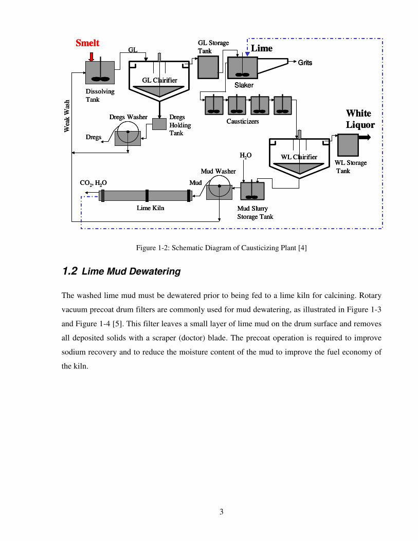
Figure 1-2: Schematic Diagram of Causticizing Plant [4]

1.2 Lime Mud Dewatering

The washed lime mud must be dewatered prior to being fed to a lime kiln for calcining. Rotary

vacuum precoat drum filters are commonly used for mud dewatering, as illustrated in Figure 1-3

and Figure 1-4 [5]. This filter leaves a small layer of lime mud on the drum surface and removes

all deposited solids with a scraper (doctor) blade. The precoat operation is required to improve

sodium recovery and to reduce the moisture content of the mud to improve the fuel economy of

the kiln.

Smelt

Dissolving

Tank

GL Storage

Tank

Slaker

Lime

Grits

Dregs

Holding

Tank

CausticizersDregs Washer

Dregs

WL Clairifier

GL Clairifier

Mud Slurry

Storage Tank

Lime KilnLime

Mud

Mud Washer

WL Storage

Tank

White

Liquor

GL

Wea

k W

ash

CO2, H2O

H2O

Smelt

Dissolving

Tank

GL Storage

Tank

Slaker

Lime

Grits

Dregs

Holding

Tank


Dregs

WL Clairifier

GL Clairifier

Mud Slurry

Storage Tank

Lime KilnLime

Mud

Mud Washer

WL Storage

Tank

White

Liquor

GL

Wea

k W

ash

CO2, H2O

H2O

Smelt

Dissolving

Tank

GL Storage

Tank

Slaker

Lime

Grits

Dregs

Holding

Tank


Dregs

WL Clairifier

GL Clairifier

Mud Slurry

Storage Tank

Lime KilnLime

Mud

Mud Washer

WL Storage

Tank

White

Liquor

GL

Wea

k W

ash

CO2, H2O

H2O

4

Figure 1-3: Rotary Vacuum Precoat Drum Filter, Courtesy of Dorr-Oliver Eimco [5]

Figure 1-4: View of Lime Mud Discharging from Lime Mud Rotary Vacuum Precoat Drum Filter,

Courtesy of Dorr-Oliver Eimco [5]

AgitatorVat

Cake Discharge

Filter Cake

Division StripsFilter Pipe

Drum

Vacuum Valve

5

Effective dewatering of lime mud is of great importance in lime kiln operation. Since heat is

required to remove water, the thermal efficiency of the kiln strongly depends on the mud solids

content, as shown in Figure 1-5 [6]. In principle, the fuel consumption of a lime kiln may be

lowered by as much as 2% for every 1% increase in the mud solids content. In practice, however,

such fuel saving is more moderate, at about 1% lower per 1% increase in solids, due to the

difficulty in controlling the temperature at the kiln feed end and keeping the residual CaCO3

content of the product lime at an acceptable level. This is particularly the case for kilns with lime

mud solids content above 75% [7]. Changes in mud solids content can cause other kiln operation

issues in addition to impacting the thermal efficiency. Lime mud with low solids content may

cause nodules (balls) with an uncalcined core and mud rings to form in/near the chain section,

while that with high solids content may result in excessive dusting and premature chain failures

associated with overheating.

Figure 1-5: Estimated Heat Consumption of Lime Kiln per Ton of Lime Mud as a Function of Dry Solids

Content in Lime Mud Feed to the Kiln [6]

1.3 Parameters Affecting Lime Mud Filtration and Dewatering

Efficiency

Many parameters influence the dewatering efficiency of the lime mud filter. These include mud

properties, white liquor properties, and equipment design and operation. For a given causticizing

system, the properties of the mud are the most important factors since they change with lime

5,200

5,400

5,600

5,800

6,000

6,200

70 75 80

He

at

Co

ns

um

pti

on

, M

J/t

Lime Mud Dry Solids, %

6

quality and dosage. Experience shows that lime mud with a slow settling rate tends to be difficult

to dewater.

The importance of particle properties on the filtration and dewatering efficiency has been

recognized since 1975 [8-12]. Studies of mineral water systems have established that the

characteristic properties of the feed slurry, such as particle charge [13-15], size distribution [16],

shape [17], hydrophobicity [18], feed slurry concentration [19], and liquid surface tension [20],

can all influence filterability.

The behaviour of particles in an aqueous system is governed mainly by their primary properties

of particle size and size distribution, shape, density, solid/liquid ratio, and surface charge. In

practice, however, it is often easier to characterize particles by measuring their macroscopic

properties such as settling rate, filterability, cake permeability, specific filtration resistance, etc.,

which in turn are related to their primary properties and to the state of the system as

characterized by the dispersion. Since the performance of dewatering equipment such as the filter

press, vacuum filter, and centrifuge depend strongly on the filterability of the feed slurry,

understanding these parameters enables operators to make adjustments to achieve satisfactory

filtration (dewatering).

Overliming is the most commonly cited cause for poor mud settling and filterability [21-22]. One

of the main issues in overliming is the high free lime (unreacted Ca(OH)2) content in the lime

mud. A common belief is that free lime particles plug the precoat filters due to their small size,

resulting in a low dewatering efficiency, and consequently lime mud with a low solids content

[22]. While overliming is highly undesirable, there is no systematic way to determine as to

whether the system is overlimed other than using the “5-minute settling test” [21].

Overliming is defined as “adding more lime to the liquor system than required”. For a given

causticizing system, the amount of lime required to achieve a targeted causticizing efficiency

may vary depending on lime quality (lime availability, reactivity, and nodule size) and liquor

quality (total titratable alkali, sulfidity, and temperature). Overliming theoretically occurs when

the liming ratio, defined as the molar ratio of CaO in lime to that of Na2CO3 in liquor, is greater

than stoichiometrically required.

7

Although many studies have been carried out to relate lime mud characteristics to the filtration

and dewatering behaviours [21-25], the mechanisms by which lime mud becomes difficult to

settle and filter are not well understood.

1.4 Objective

The objective of this research was to develop a fundamental understanding of the impact of

liming ratio on settling rate and filterability of lime mud produced in the kraft chemical recovery

process. In order to achieve this, a systematic study was conducted to investigate the effect of

liming ratio on the causticizing efficiency (CE) values, physical characteristics (e.g., size

distribution), as well as settling rate and filterability of the precipitated mud using different

sources of lime. The ultimate goal was to develop an analytical technique to detect an overlimed

condition that can be readily integrated into the operations of a causticizing plant.

1.5 Structure of Thesis

This document contains seven chapters. Chapter 1 gives a general overview of the kraft pulping

process and lime mud dewatering in a causticizing plant and introduces the objectives of the

thesis.

Chapter 2 is a review of relevant literature pertaining to this study. In Chapter 3, experimental

methodology and measurement techniques are outlined. The results of the experiments and the

related discussions are presented in Chapter 4. The mathematical technique used to predict a

batch settling curve is described in Chapter 5. Chapter 6 highlights the practical implications of

this study. Finally, Chapter 7 summarizes major conclusions drawn from the work, and explores

further research possibilities.

8

2 Literature Review

An important step in the chemical recovery process involves the dewatering of calcium

carbonate (lime mud) particles that have been separated from the causticized liquor (white

liquor). Effective dewatering of lime mud is an important objective for both energy and chemical

savings in the operations of a pulp and paper mill.

The separation of lime mud from the white liquor involves two stages after the slaking and

causticizing reactions. First, the white liquor, which contains mainly NaOH and Na2S, is

separated from CaCO3 particles in a sedimentation clarifier or a pressurized filter to achieve a

high-clarity white liquor. Then, a vacuum precoat filter washes and dewaters the lime mud

before it is fed to the lime kiln. The solids content of the lime mud after filtration is typically

about 75 %, but may vary between 60% and 85% [7].

This chapter reviews the major factors affecting the settling and dewatering of lime mud

including solid and liquid properties, operational variables, and equipment design and

performance.

2.1 Settling Theory

Sedimentation typically involves the separation of particles from a fluid by gravity. Particle size,

particle density, and fluid viscosity are the primary factors to consider in a sedimentation

process; however, particle concentration, shape, and surface charge can also have a significant

influence. Free settling, or dilute suspension, is the case in which the particles are able to settle

individually. Hindered settling, or thickening, is the term used to describe settling behaviour at

high particle concentrations, in which sedimentation rates are tied to the concentration and the

state of aggregation of the particles rather than to particle size [26].Very fine particles (a few

micrometers) settle slowly by gravity alone. However, if they aggregate, the settling rate is

considerably higher.

The original theory describing the movement of a particle in an infinite fluid was derived by

Stokes [27]. The terminal velocity of a spherical particle (ut) in the laminar flow regime as

derived by Stokes is given by:

9

( )µ

ρ−ρ=

18

gdu s

2

t

(1)

where

µ: Liquid viscosity (Ns/m2)

ρ: Liquid density (kg/m3)

ρs: Solid density (kg/m3)

g: Gravity acceleration (m/s2)

d: Particle diameter (m)

In practice, many factors other than those included in the above equation can also influence the

flow behaviour and hence the terminal velocity of particles. They can be divided into those

depending on particle properties and those depending on the flow system. Various refinements

have been made to the Stokes equation. However, still there remains a common shortcoming

which is the assumption that a particle settles freely without interference from other particles.

When the particle concentration is sufficiently high, the particles can no longer settle freely. For

a non-flocculated system, Richardson and Zaki [28] compared sedimentation and fluidization

processes and showed that the settling velocity is related to the terminal settling velocity of the

particles and the porosity raised to a power that is a function of the particle Reynolds number:

n

tuU ε=

(2)

where

U: Settling velocity of particle suspension (m/s)

ut: Terminal velocity (m/s)

ε: Porosity

The exponent n varies from 2.39 to 4.65 depending on the particle Reynolds number and the

diameter of the vessel in which sedimentation is taking place [26].

10

A settling test can be used in the design of a sedimentation clarifier or thickener. In such tests, a

slurry of known initial concentration is allowed to settle. As the settling process proceeds, a clear

interface appears between the slurry and the supernatant. By plotting the height of the interface

with time, the settling velocity can be obtained from the initial slope of the settling curve.

The type of settling behaviour demonstrated by suspended solids depends largely on the initial

solids concentration and their tendency to flocculate. The first general study of flocculated

suspensions was carried out by Coe and Clevenger [29]. They concluded that a concentrated

suspension may settle in one of two different ways depending on the initial solids concentration.

In Type I settling, the sedimentation rate progressively decreases throughout the process. This

type of settling is obtained in a dilute suspension, where particles have little interaction with one

another as they settle. In Type II settling, particles flocculate as they settle. This type of settling

usually occurs when the initial particle concentration is high. A detailed description of these

settling types is included in Appendix A.

Dorris and Allen [23] proposed that lime mud mixtures typically fall in the category of dilute

slurries that undergo Type I settling.

2.1.1 Mathematical Model for Batch Settling

Holdich and Butt [30] proposed a mathematical model to predict the results of a batch settling

test. They performed settling experiments on talc particles suspended in water at different initial

concentrations and obtained settling plots from performing conductivity measurements as the

suspensions settled. Their method is in-line with the belief that the settling rate is only a function

of solids concentration according to Kynch theory, which is described in the following section.

2.1.1.1 Kynch Theory

The theory of batch settling is credited mainly to Kynch [31]. It begins with the assumption that

the particle settling flux G is a linear function of only the settling rate U and the solids

concentration C:

UCG =

(3)

11

In a time interval (∂t), the accumulation of particles in the interfacial layer is given by the

difference in input and output fluxes, as shown in Figure 2-1:

Figure 2-1: Flux Variations during Batch Sedimentation

( )dhA

t

CAdh

h

UCUCUCA SSS ρ

∂

∂=ρ

∂

∂+−ρ (4)

where

C: Solids concentration by volume fraction

A: Cross-sectional area of vessel (m2)

h: Height of vessel (m)


U: Settling velocity (m/s)

Thus, the rate at which a known concentration propagates through the settling vessel can be

calculated as a function of the change in the solid flux relative to the solids concentration [26]:

( )C

UC

t

h

∂

∂−=

∂

∂ (5)

As the solids settle the concentration increases towards the bottom of the settling vessel, causing

the interface between the clear liquid and the settling solids to move downward. The change in

the height of this interface with time is known as the batch settling curve. Equation (5) shows

that the settling velocity (U) is affected by the solids concentration.

Clear Liquid

Settled Solids

h hh+dh h+dh

SUCAρ

( )SA]dh

h

UCUC[ ρ

∂

∂+

Clear Liquid

Settled Solids

h hh+dh h+dh

SUCAρ

( )SA]dh

h

UCUC[ ρ

∂

∂+

12

According to Kynch’s 1952 idealized concept of batch thickening, layers at each particle

concentration propagate at a characteristic upward velocity and eventually intercept the interface.

At the time of the interception, the interface assumes a settling velocity characteristic of the

propagated concentration. When the maximum concentration reaches the interface, no further

settling is possible. The interface velocity is constant until the first propagating layer reaches the

interface, at which time the velocity begins a steady decline to zero. The first decreasing rate

period is explained by Kynch theory as the propagation of higher concentration layers from the

bottom to the interface.

Subsequently, the value of the propagation velocity is fixed, causing layers of constant

concentration propagating from the origin to the settling interface curve, called “concentration

characteristics” [26]. The interface settling curve and the concentration characteristics during the

settling of a suspension are shown in Figure 2-2. In the concentration characteristics region, a

mass balance on a solid layer shows that the solid output is less than the solid input due to the

concentration increase.

Figure 2-2: Solids Concentration Characteristics during Settling

2.1.1.2 Theoretical Batch Settling Curve

The deduced settling and propagation velocities can then be used to predict the batch

sedimentation curve under any operating condition, e.g., a change in concentration [30].

In the settling of concentrated suspensions the following force-momentum balance applies [32]:

0

2

4

6

8

10

12

14

0 10 20 30

He

igh

t o

f In

terf

ac

e, c

m

Sedimentation Time, min

Interface Settling Curve

Concentration Characteristics

Solids In∂h

Solids Out, Less than Solids In, due to a

Concentration Increase

Solids In= Solids Out

13

( ) Uk

Cgx

Ps

s µ−ρ−ρ=

∂

∂ (6)

where

Ps: Solids compressive pressure (N/m2)

C: Solids concentration by volume fraction

g: Gravitational constant(m/s2)

ρ: Fluid density (kg/m3)


µ: Fluid viscosity (Ns/m2)

k: Permeability (m2)

U: Settling velocity (m/s)

For homogeneous systems, the particles do not separate from the continuous phase (such as

water), but cause a change in the properties of the continuous phase, for example buoyancy and

viscosity. These considerations are therefore relevant to certain situations, such as where the

suspension needs to flow within a pipe [32].

The left hand side of Equation (6) may be considered to be a reaction force due to particle-

particle contact. The first term on the right side is the gravitational force, and the remaining term

is the liquid drag force on the particles [26]. Under the conditions where the particle

sedimentation does not possess a continuous contact of solids, the stress gradient becomes zero

[33] and Equation (6) can be rearranged to provide:

( ) µρ−ρ= /kCgU s (7)

Here, parameter k is permeability (m2) that can be calculated from:

( ) 2

v

2

3

S1Kk

ε−

ε= (8)

where

K: Kozeny coefficient

Sv: Specific surface area per unit volume (m2/m

3)

ε: Local porosity (1-C)

14

The specific surface area may be calculated by 6/(dp×ψ). Where dp is particle diameter and ψ is

the sphericity. Hence, substituting k in Equation (7) with Equation (8) results in:

µ

Ψ−ρ−ρ=

K36

d)C1)((gUC

223

s (9)

Differentiating Equation (9) provides an expression for the propagation velocity of a

concentration characteristic:

µ

Ψ−ρ−ρ−=

K36

d)C1)((g3

dt

dh222

s (10)

This method assumes that the initial concentration is uniform (after a short time, it increases

from the bottom of the suspension) and that the settling velocity becomes close to zero at the

same time that the concentration approaches a maximum value relating to that of the sediment

layer deposited at the bottom of the vessel.

Holdich and Butt [30] suggested that the height of the interface between the supernatant clear

liquid and the settling suspension can be predicted using Equations (7) and (10) and employing a

K of 5 in fixed or slowly moving beds and of 3.36 in settling or rapidly moving beds. However,

there is experimental evidence to suggest that K may not have a constant value and could depend

on various parameters such as concentration, particle size and shape, tortuosity, and wall effects

[33, 34]. Moreover, when particles are smaller than 10 µm, the surface charge on the particles,

which is often represented by zeta potential, becomes more important [35]. None of the above

equations include zeta potential effects on the batch settling rate of particles.

It is apparent that the Holdich and Butt model is constrained by certain limitations because (1) K

cannot be a fixed value and (2) the interparticle interactions affecting the particle packing and the

final settled sediment concentration should also be considered.

2.2 Filtration Theory

The separation of solids from a suspension by means of a porous medium or screen which retains

the solids and allows the liquid to pass through is termed filtration. There are two basic types of

filtration. In the first type, frequently referred to as cake filtration, particles from the suspension

are deposited on the surface of a porous septum which provides only a small resistance to flow.

15

As the cake gradually builds up on the filter medium, the resistance to flow progressively

increases. In the second type of filtration, depth or deep-bed filtration, the particles penetrate into

the pores of the filter medium. This configuration is used for the removal of fine particles from

very dilute suspensions.

Many equations are used in filtration characteristic studies. The best known theoretical model for

the filtration process is Darcy’s equation. By integrating Darcy's law under conditions of both

constant pressure and cake permeability, Holdich [36] showed that,

pA

RV

kpA2V

t m

2 ∆

µ+

∆

µβ= (11)

where

t/V: Filterability (time required to filter a “V” volume of filtrate)

µ: Fluid viscosity (Ns/m2)

∆p: Pressure drop across cake and cloth (N/m2)

A: Filter area (m2)

k: Cake permeability (m2)

Rm: Medium resistance (m-1

)

β: Cake-to-filtrate volume ratio

β can be calculated from the following:

β =ρls

1− s( )Cρs − 1 − C( )ρls (12)

where

s: Solid mass fraction (%w/w)

C: Cake solids concentration by volume fraction

ρl: Density of liquid (kg/m3)

ρs: Density of solids (kg/m3)

Data obtained from vacuum filtration tests are used to calculate filtration parameters, such as

cake permeability and cloth resistance, using a common method of plotting t/V as the dependent

variable against V, as the independent variable, and drawing a best fit line through the data. The

line of best fit on this plot has a slope of

16

kpA2 2∆

µβ (I)

and the intercept on the t/V axis occurs at

pA

Rm

∆

µ (II)

Thus, the permeability k and medium resistance Rm can be calculated by rearranging terms (I)

and (II), if all other parameters in these equations are available.

The permeability of a filter cake is the most important factor in cake filtration (in relation to

design and scale-up) and is often interpreted through a measure of the cake’s specific resistance.

The specific resistance (αav) of a filter cake is a measure of the resistance to fluid flow through

the cake. It is inversely proportional to the permeability of the filter cake, shown by the relation

Ck

1

s

avρ

=α

(13)

According to the Carman-Kozeny equation [37], the specific resistance is inversely related to the

square of the particle size; hence, it increases as the particle size decreases, as shown below:

32

avs

av

1

d

180

ε

ε−×

ρ=α (14)

where dav and ε are the average particle size diameter and porosity of the filter cake, respectively.

Theliander [38] found that the specific filtration resistance and the porosity of a lime mud filter

cake changes with the filtration pressure, and concluded that lime mud is a compressible

material. He also found that the lime mud particles are agglomerates of smaller particles with a

variety of different shapes and sizes. The porosity of the filter cake is also a function of the

particle size distribution. When the size distribution is wider, smaller particles can occupy spaces

between larger ones and the particles are able to pack together more tightly, forming a dense

cake.

17

In addition to the above factors, the electrokinetic forces among particles play an important role

in the particle packing. The zeta potential (ζ) is often used to characterize the surface electrical

charge of colloidal size particles in a slurry [39]. The ζ determines the electrostatic forces

between particles, which significantly affects both the properties of the slurry prior to slurry

filtration and the filter performance during the filtration process. The interaction forces between

the particles can become as significant as gravitational and hydrodynamic forces, especially for

particles smaller than 10 µm, which interact more with the surrounding fluid [35].

2.3 Forces Involved in Aggregation/Dispersion

Most early attempts to explain the stability of a suspension considered only the surface charge of

the particles. The existence of a charge was recognized as the primary cause of stability. Thus

neutralization of the charge would lead to aggregation. Until recently, it was believed that only

two forces operate between surfaces in a liquid such as water: the attractive Van der Waals force

and the electrostatic “double layer” force. These forces can be attractive or repulsive, and

together they form the basis of the Derjaguin-Landau-Verwey-Overbeek or DLVO theory [40].

2.3.1 Van der Waals Forces

The Van der Waals force is the term commonly used to refer to a group of electrodynamic

interactions that occur between the molecules in two different particles. Dispersion forces make

up the dominant contribution to the Van der Waals interaction between two particles. At a certain

separation distance, the mutually repulsive force of electrons is lessened and weak bonds can be

formed. These are Van der Waals interactions.

Although the calculation of Van der Waals forces between spherical particles is mathematically

complex, the resulting equation for equal-size spheres is simple as shown in Equation (15) [41]:

1

HAd12

rAV −= (r>>d) (15)

where VA is the interaction energy between spheres of radius r (mm), d1 (nm) is the distance of

the closest approach between the spheres, and AH (J) is the Hamaker constant. It is difficult,

18

however, to determine the Hamaker constant, but tables of Hamaker values for some systems

are available [42] and values are generally found to be in the range of 0.1×10-20

to 10×10-20

J.

2.3.2 Electrostatic Forces

The aggregation of colloids is known as coagulation or flocculation. Repulsion is not due

directly to the surface charge on the solid particles, instead it is the interaction between their

respective double layers. Particles are subjected to random movements due to Brownian motion

and mixing effects. This brings some particles into close proximity to allow the attractive surface

forces to bind them into aggregates. If the surfaces of the particles are charged, the resulting

repulsive force may be sufficient to prevent aggregation. Chemical additives can also be used to

alter the surface charge to either promote or prevent aggregation.

There are two forms of aggregation (coagulation) related to electrical effects. If the surface

charge is brought near zero, the force of repulsion is lost and particles can aggregate. This is

referred to as homo-coagulation as the particles are generally of the same type. Hetero-

coagulation occurs when different particles have an opposite charge and a positive force of

attraction induces aggregation [43].

Electrical charge can be generated on a solid surface by a number of mechanisms. These include

specific chemical interactions, preferential dissolution of surface ions, and lattice substitutions.

2.3.2.1 Development of Electrical Double Layer

During the development of an electrical surface charge, the solid surface acquires a potential

with respect to the solution. The surface charge is compensated by an equal charge distribution in

the aqueous phase. The charge in the solution together with the charge on the solid surface is

referred to as an “electrical double layer”. The thickness of this layer depends upon the type and

concentration of ions in the solution. A schematic representation of the potential drop across the

double layer is presented in Figure 2-3.

19

Figure 2-3: Gouy-Chapman Model with Stern Modifications [44]

Various models have been developed to describe the structure and properties of the double layer.

Some models require several experimentally-derived parameters. The Gouy-Chapman model for

a diffusive double layer is a facile model that has shown good performance [45].

In 1924, Stern [46] introduced a modification to the Gouy-Chapman model. He proposed that the

thickness d of the Stern layer is the closest distance to the particle surface that an ion can

approach without undergoing specific adsorption. The DLVO theory describes the tendency of

colloids to agglomerate or remain discrete by using the net interaction energy profile, which is a

combination of the Van der Waals attraction profile with the electrostatic repulsion profile.

Figure 2-4 shows a typical interaction energy profile. The net interaction profile is formed by

subtracting the attraction profile from the repulsion profile. The point of maximum repulsive

energy is called the energy barrier.

+ −

−

−

−

−

−−

− −

++

+

+

+

+−

−−

−

Po

ten

tia

l

Distance from the Particle Surface

Potential at shear plane = ζ= ζ= ζ= ζ

Stern Plane

Shear Plane

Surface Potential

Diffuse Layer

ψψψψ0000

d

20

Figure 2-4: Interaction Energy Profile

The height of the energy barrier indicates the stability of the system. In order to agglomerate, two

colliding particles must have sufficient kinetic energy from their velocity and mass to overcome

this energy barrier. If the barrier is cleared, then the net interaction is attractive and, as a result,

the particles agglomerate. This inner region is often referred to as an energy trap because the

colloids can be considered to be trapped together by Van der Waals forces. The energy barrier

can be altered by changing the ionic environment, pH, or by adding surface active materials to

directly affect the charge of the colloid. In each case, zeta potential measurements can indicate

the impact of the alteration on the overall stability.

2.3.3 Zeta potential (ζζζζ)

Most fine particles in contact with a liquid acquire an electric charge on their surfaces. Zeta

potential (ζ) is an indicator of the charge that can be used to predict and control the stability of

suspensions or emulsions. The ζ is the potential difference across the diffuse layer of double

layer that surrounds a particle. It is responsible for the electrokinetic behaviour of the particle

under an electric field. According to the double layer theory, the ζ may be equated to the Stern

layer potential (ψ), and the sign and magnitude reflect the type of ion that forms the double layer.

Surface charge is important with regards to the suspension stability, rheology, sediment

characteristics, and other surface-driven phenomena. Since the ζ is the potential measured at a

certain distance from the particle surface as shown in Figure 2-3. It does not correspond directly

to the potential at the particle surface. It is a function of the surface charge of the particle and the

nature and the composition of the surrounding suspension medium.

Van der Waals AttractionInte

raction E

nerg

y

Electrical Repulsion

Net Interaction Energy

Distance Between Colloids

Van der Waals AttractionInte

raction E

nerg

y

Electrical Repulsion

Net Interaction Energy

Distance Between Colloids

21

Instruments to measure zeta potential are based on one of the following principles: a)

electrophoresis - the movement of charged particles relative to the surrounding under an applied

field; b) electro-osmosis - the movement of the liquid relative to a surface charge; c) streaming

potential - the electric field created when a liquid flows along a stationary charged surface; and

d) sedimentation potential - the electric field created when charged particles move relative to a

stationary liquid [47]. Most zeta potential measurements today are carried out on small particles

in dilute suspensions using the electrophoresis technique. For concentrated suspensions,

instruments have been developed using electric and ultrasonic impulses to determine zeta

potential values [48].

If an electric field is applied across a suspension of small particles, the particles will tend to

move toward either the anode or the cathode depending on whether the solid surface carries a

positive or negative charge. The migration speed “Ue” (electrophoretic velocity or mobility) of

the particles is directly proportional to the magnitude of the zeta potential. An equation proposed

by Smoluchowski relates the mobility to zeta potential [49].

µπ

=ζD

4U e

(16)

where µ represents the viscosity and D the dielectric constant of the medium.

For practical purposes, the magnitude of the net repulsive force between particles is represented

by the zeta potential. Wakeman [35] proposed the following statements about the role of zeta

potential in a solid/liquid separation:

a) Increasing the solids content in a solid/liquid mixture increases the net repulsive force between

the particles.

(b) Increasing ζ increases the net repulsive force between the particles.

(c) Decreasing the magnitude of the repulsive force causes the dispersion to become unstable.

This causes particles to agglomerate and settle more easily.

22

(d) Repulsive forces can be decreased by either adding a non-adsorbing electrolyte to the liquid

to change the distribution of solution around ions, or by altering the electrical charge on the

surface of particles through the specific adsorption of certain ions or charged polymers.

Wakeman also stated that understanding the link between the ζ and separation characteristics,

such as cake formation rates and settling rates, can often shorten testing plans when evaluating

the separability of new suspensions. As a result, around the isoelectric point of the suspension

(close to ζ ≈ 0 mV), one can expect faster settling rates, more rapid filter cake formation, and

slightly higher moisture content in cakes and sediments, due to the aggregation of particles in the

suspension when the interparticle repulsion forces are small. At the maximum or minimum ζ,

one can expect slower settling rates, slower cake formation rates, and slightly lower moisture

content in cakes and sediments, due to the existence of greater repulsive forces causing a more

stable dispersion of particles in the liquid.

2.4 Correlation Between Sedimentation Volume and Colloid Stability

It has long been recognized that there is a close correlation between sedimentation volume and

colloid stability [50]. When a well-dispersed solution settles, it does so slowly and tends to form

a dense deposit. A coagulated sol (a stable colloidal solution), on the other hand, settles rapidly

because of the formation of aggregate particles, and the final sediment volume is large because

the aggregates form porous structures as they adhere at the point of first contact.

Michaels and Bolger [51] showed that the final sediment height Zf was determined by the

volume fraction of flocs in the suspension (φF) and the initial sediment height Z0 for aqueous

kaolinite suspensions according to the following equation:

Const62.0

ZZ F0

f +φ

= (17)

Gaudin and Fuerstenau [52] and Firth [53] confirmed the same relationship for a CaO and TiO2

suspension, respectively.

The density of the flocs is measured by the floc volume ratio CFP= φF/φP where φF is the volume

fraction of flocs and φP is the volume fraction of particles. Loosely packed flocs (large CFP) are

23

expected to occur in systems with very strong attractive forces between the particles; as the

attractive forces diminish, the floc must become more compact to withstand the initial very high

shear rate to which it has been subjected (γ• CFP). Firth and Hunter [54] successfully describe the

rheological behaviour of coagulated solutions as shown in Equation (18).

( )

ξ−

γη=

•

2

12

1

H

C0

FP dBd12

A

r20

1C

FP

(18)

where

CFP: Floc volume ratio

AH: Hamaker constant

d1: Distance at which force between particles is a maximum (nm)

B(d1): Function of separation between particles

r: Particle radius (mm)

γ•CFP: Shear rate (s

-1)

η0: Viscosity of suspension medium (Ns/m2)

The bracketed term is a measure of the maximum force that can be withstood by the bond

between two particles. This equation suggests that the relative sediment height after a fixed time

interval (i.e., Zf/Z0) would decrease as ζ2 decreases [55]. The settling velocity also clearly

depends on the degree of aggregation of the system. Fuerstenau et al. [56] used this equation as a

technique for locating the point of zero charge or isoelectric point of their systems. Also, the

correlation between isoelectric point and the settling time for an alumina sol is well demonstrated

in the work of Yopps and Fuerstenau [57].

2.5 Influence of Particle Properties on Lime Mud Dewatering

As noted in Section 1.3, the performance of dewatering equipment such as the filter press,

vacuum filter, and centrifuge greatly depends on the filterability of the feed slurry. The filtration

and dewatering efficiency, on the other hand, are strongly influenced by the particle properties.

As a result, knowledge of particle properties enables the improvement of the separation and

dewatering processes.

24

Lime mud consists mainly of small calcium carbonate particles with some impurities

(approximately 7-10 %). The particles are agglomerates of crystallites, which are approximately

10-30 µm in diameter. Calcium carbonate has three polymorphs; calcite, aragonite, and vaterite

[58]. Investigation of the crystallinity of lime mud reveals only calcite structures [59].

2.5.1 The Calcite/Water System

The development of surface charge on calcite is a complex phenomenon and has been discussed

in detail by Hanna and Somasundaran [60]. The thermodynamics of calcite dissolution in an

aqueous solution are fairly well known [61-64]. First, the surface charge is developed by the

preferential dissolution of its constituent species. Second, various complexes of charged species

result from the hydrolysis reaction of the constituent ions [62]. The surface of calcite is not static.

Continuous dissolution and reprecipitation of ions take place, and thus proton and hydroxide ions

play a dual role in the determination of the surface potential of calcite [65]. Proton and hydroxide

ions affect the surface charge by changing the dissolution balance of calcite, and to some degree,

by direct adsorption onto the surface. The fundamental charged groups at the surface are the

lattice ions, i.e., Ca2+

and CO32-

, which may be protonated or hydroxylated. Calcite in aqueous

dispersions tends to aggregate strongly and in many applications the particles need to be

stabilized in the dispersed phase.

2.5.2 Zeta Potential of Calcite

Although published studies on ζ have provided insights into the surface charge of calcite, they

are also somewhat contradictory. In some studies only positive or negative values are obtained,

while in other studies the isoelectric point (IEP)2 values range from 5.4 to 11. Many explanations

have been given to account for this behaviour. Berlin and Khabakov [66] suggest that the

electrical charge depends mainly on the nature of the calcite sample. According to Siffert and

Fimble [67] the observed differences in ζ can be explained by differences in the solid:liquid ratio

of the suspension, by vigorous shaking, and by the presence of atmospheric CO2. Several

researchers [68-70] suggested that in a pure aqueous suspension of calcite, Ca2+

and CO32-

species are the potential-determining ions (PDI). In other studies, it is shown that H+, OH

-,

CaOH+, and HCO

-3 ions also can act as potential determining ions [62, 64]. If other ions are

present in the aqueous suspension, the surface charge may change depending on the type of ion

2 IEP is defined as the pH at which a particular molecule or surface carries no net electrical charge.

25

and its concentration [64, 68]. The PDIs bond directly to the calcite surface sites. The surface

density of these PDIs is lower than that of -Ca and -CO3-CO3 sites on the crystal surface [71].

Most likely, Ca2+

and CO32-

have the same affinity for the calcite surface. Thus the zero ζ for

calcite occurs when the concentration of Ca

2+ ions in the suspension equals the concentration of

CO32-

ions [61]. Because the magnitude of the ζ depends on the actual Ca2+

and CO32-

concentrations, the ζ measurement is sensitive to the dissolution rate of calcite. At a high

dissolution rate, the Ca2+

concentration equilibriates rapidly; the ζ measurement is not sensitive

to equilibrium time. Whereas at a low dissolution rate, the Ca2+

concentration changes over time

and the ζ changes with time [61]. Stipp and Hochella [72], based on results of their study using

X-ray Photoelectron Spectroscopy (XPS) and Low Energy Electron Diffraction (LEED), showed

that pure CaCO3 in water contains HCO3- and CaOH

+ functional groups at the surface.

Several researchers investigated the influence of PCO2 on the surface charge of calcite [62, 63].

They concluded that the effect of pH and PCO2 on zeta potential is indirect, as they act only as a

determinant for Ca2+

and CO32-

concentrations in the suspension. As a result, in an open system,

the measurements are sensitive to CO2 variations in the air, and hence the equilibrium time and

the stirring rate [54].

2.5.3 Influence of Inorganic Ions on the Surface Charge of Calcite

The role of dissolved mineral species in determining the surface charge generation of calcite in

aqueous solutions has been discussed in several investigations [68-70]. Generally, polyvalent

ions (e.g., PO4 3-

, HPO4 2-

, SO4 2-

, CO3 2-

, Mg2+

, Ca2+

) change the surface charge of calcite due to

adsorption onto oppositely charged surface sites and/or precipitation of other minerals onto the

calcite surface. Furthermore, Foxall et al. [69] and Thompson and Pownall [70] each showed

Ca2+

to be the potential-determining cation of calcite. However, several researchers [72-74] argue

that H+, OH

-, CaOH

+, and HCO3

- ions can also act as PDIs. For example, adding Na2CO3 to the

calcite suspension makes the zeta potential increasingly negative [75]. Fuerstenau et al. [75]

found that the zeta potential at the calcite/solution interface was sensitive to changes in both pH

and aqueous carbonate concentration. In the presence of a dilute solution of sodium carbonate

(10-3

M), a positive ζ of calcite decreased.

While the effect of Ca2+

concentration in suspension on the surface charge has been the subject of

a number of investigations, the effect of carbonate ions does not seem to have received the same

26

attention. The Ca2+

concentration has a profound effect on the zeta potential [68-69, 72]. The

overall conclusion in these studies is that increasing Ca2+

concentration causes zeta potential to

shift to more positive values due to Ca2+

adsorption to the negative sites on the calcite surface.

2.6 Lime Mud Settling and Filterability - Previous Studies

This section reviews major parameters affecting the settling and dewatering of lime mud in the

pulp and paper industry. These include lime properties, liquor properties, operation variables,

and equipment design.

2.6.1 Definitions

The terms used to characterize the green liquor and white liquor in the pulp and paper industry

are causticizing efficiency (CE), total titratable alkali (TTA), and sulfidity. Liming ratio also

refers to an operating parameter in the causticizing plant.

2.6.1.1 Causticizing Efficiency

An operating parameter used in kraft pulp mills to indicate the extent of production of NaOH in

the causticizing reaction is known as causticizing efficiency (CE), defined as:

[ ] [ ]

100CONaNaOH

]NaOH[CE

32

×+

= (19)

where [NaOH] and [Na2CO3] are sodium hydroxide and sodium carbonate concentration,

respectively. All chemical concentrations are expressed as equivalent grams of Na2O per liter of

solution.

The NaOH concentration in the above equation refers to the product of the causticizing reaction.

Thus, when dealing with systems in which Na2S is present, the NaOH produced from the

hydrolysis of Na2S should be taken into account.

2.6.1.2 Total Titratable Alkali and Active Alkali

Total titratable alkali (TTA) is the total concentration of NaOH, Na2S, and Na2CO3 in green and

white liquors. TTA is defined as the total molar concentration of these chemicals, expressed as

27

the equivalent mass of Na2O per unit volume of the solution (i.e., gNa2O/L solution). The value of

TTA remains constant throughout the process. Initially, it is the amount of Na2CO3 and Na2S that

are put into the reaction. As the reaction progresses, the carbonate is converted into hydroxide,

while the sulphide is unchanged. TTA is defined mathematically as

TTA = [NaOH] + [Na2CO3] + [Na2S] (20)

Active Alkali (AA) is mathematically defined as follows:

AA = [NaOH] + [Na2S] (21)

2.6.1.3 Sulfidity

Sulfidity refers to the relative amount of sodium sulphide present in the system. There are two

main ways of calculating sulfidity, one is based on TTA and the other on AA of the solution,

since the value of AA is necessarily lower than TTA, and the sulfidity on AA is about 4% higher

than that on TTA. The sulfidity definition based on TTA is the molar concentration of Na2S in

green liquor divided by the TTA, expressed as equivalent grams of Na2O per liter of solution:

100]SNa[]CONa[]NaOH[

]SNa[%Sulfidity

232

2 ×++

= (22)

The sulfidity definition based on AA is

100]SNa[]NaOH[

]SNa[%Sulfidity

2

2 ×+

= (23)

2.6.1.4 Liming Ratio

The liming ratio (LR) refers to the molar ratio of CaO in the lime to that of Na2CO3 in the liquor.

In the causticizing reaction, one mole of Na2CO3 reacts with one mole of Ca(OH)2 to produce

two moles of NaOH and precipitate one mole of CaCO3. Therefore, overliming occurs when the

liming ratio (molar ratio of CaO/Na2CO3) is greater than stoichiometrically required. In theory,

adding more than one mole of lime for every mole of Na2CO3 would overlime the system,

28

resulting in unreacted lime that would create costly problems with settling and filterability as

well as ring formation.

Similarly, under-liming occurs when the amount of lime added is less than stoichiometrically

required.

2.6.2 Physical Properties of Lime and Lime Mud

The quality of white liquor and the efficiency of the causticizing plant are influenced by the

physical properties of quicklime (CaO) and lime mud [76]. It is known that the particle size of

lime mud influences the kinetics of the causticizing reaction [77] as well as the separation

properties of the lime mud formed [38].

Kokkila and Lappas [78] observed that lime mud particles have rough surfaces. Adsorbed water

was found on the surface irregularities, and the average thickness of the water layer was

independent of the particle size. As a result of theoretical and experimental investigations, they

concluded that the filtration of lime mud was noticeably improved with increasing particle size.

Dorris [24] studied the particle size and specific surface area of dispersed lime mud particles in

the white liquor produced by the slaking and causticizing reactions. He found that several

structural changes took place during the reaction. Calcium hydroxide particles were smaller and

had a more irregular shape compared with reburned lime and lime mud particles. Angevine [79]

suggested that the particle size of lime mud is strongly dependent on the slaking reaction

conditions. Dorris and Allen [23, 80] reported that the lime mud settling rate was inversely

proportional to the specific surface area of calcium oxide and that the type of lime has an effect

on the settling rate of lime mud.

2.6.2.1 Lime Quality

Lime reburning is the process of converting lime mud (mostly CaCO3) generated in the

causticizing plant into reburned lime (CaO). The calcination reaction takes place at high

temperatures (> 800 °C) in the lime kiln.The quality variations in the reburned lime can cause

problems during green liquor slaking, causticizing, and lime mud settling processes. Ideally,

reburned lime should be soft, and consist of 2 cm-diameter pebbles [81]. Typically, the specific

surface area of reburned lime is smaller than 0.5 m2/g whereas for pure lime, it is smaller than 2

m2/g. The quality of reburned lime is judged in terms of lime availability, residual calcium

29

carbonate, and reactivity. Availability refers to the fraction of lime (as CaO) in the reburned lime

available for slaking and causticizing. Pure lime will have an availability of nearly 100%.

Reburned lime has an availability of 87-92% [81].The calcium oxide in the reburned lime must

slake quickly in the green liquor slaker to ensure white cooking liquor causticity targets. A

highly reactive lime typically has a porous structure, and slakes within 5 minutes [81].

Sylwan [82] reported that the physical properties (i.e., porosity and surface area) of the lime may

play an important role in the causticizing reaction. Based on an experimental study made on two

reburned lime samples, Rydin [83] proposed a kinetic model of the slaking and causticizing

reactions and concluded that the rate of the causticizing reaction was governed by the physical

properties of the lime. Many researchers [84-85] have found that the causticizing efficiencies

and settling rates of lime mud varied significantly with the type of lime. Angevine [21] suggested

that fresh and reburned limes should be stored in separate silos to eliminate problems caused by

the difference in reaction rates.

The effect of calcining temperature on lime quality was reported in earlier investigations [86-87].

Kinzner [86] showed a minimum in the mud settling rate at lime reburning temperatures around

1100 °C. He found a decrease in the causticity (i.e., lower yield in the causticizing reaction)

when the lime was calcined at temperatures above 1100 °C. Dorris and Allen [23] characterized

the chemical and physical properties of reburned lime samples from 10 Canadian kraft mills. The

reburned lime samples were then compared in laboratory tests on the basis of their rates of

slaking, causticizing and mud settling. They found that all reburned limes had low reactivity with

water, despite their high porosities. The reason for this discrepancy is that for quicklime a large

surface area often accompanies a high porosity (i.e., for a porosity of 45%, a surface area of 10

m2/g). This is not the case for reburned limes, which had much lower surface areas. They

concluded that at low calcining temperatures, the rate of sintering is low and thus the lime

structure is made up of a large number of small crystallites. As a result, the lime has a high

specific surface area and is chemically reactive (soft-burned limes). On the other hand, when the

temperature and duration of calcinations increases, pores coalesce, the crystallites grow, which

causes a decrease in the surface area, and the reactivity of the quicklime decreases (hard-burned

lime). Dorris and Allen [23] studied lime mud settling as a function of the slaking time. They

reported that despite the scatter in the data, reburned lime samples, which had a lower rate of

slaking (i.e., long slaking times), settled more rapidly. Therefore, reasonably reactive limes

30

appear to offer the best compromise for most mills between reactivity and the rate of lime mud

settling. Kinzner [86] observed the same properties for calcined limestone.

Dorris [88] investigated the combined effects of mud washing and calcining conditions on the

properties of reburned lime and lime mud. He found that the temperature and time of calcination

have a more significant effect on the properties of reburned lime than does the amount of water-

soluble sodium in the mud prior to the calcination. In the temperature range between 1000 and

1200 °C, the lime reactivity is high and practically independent of the calcination time and

degree of mud washing. The reactivity of reburned lime decreased markedly above 1300 °C for

well-washed mud and above 1,200 °C for poorly washed mud.

2.6.2.2 Chemical Composition of Lime Mud

The presence of non-process elements (NPE) in lime mud is widely acknowledged to have a

negative effect on mud settling, mud filterability, and lime reburning. Lime mud containing NPE

has a lower dry solids content and a higher alkali content.

The physical properties of lime and lime mud change when they contain more inert compounds.

Therefore, filtration cannot properly dewater this type of lime mud. This causes the feed to the

lime kiln to contain more water, and the kiln energy consumption increases because of a much

higher heat requirement for evaporation.

Most typical NPE in the lime cycles are magnesium (Mg), aluminum (Al), silicon (Si),

phosphorus (P), iron (Fe), manganese (Mn), sulphur (S), sodium (Na), potassium (K), and

chlorine (Cl). Makeup lime and process water contribute significantly to quantities of NPE. Their

concentrations vary from one mill to another depending on the type of materials and the degree

of closure [89].

Keitaanniemi and Virkola [90] characterized NPE according to their tendency to accumulate in

the liquor cycle. K and Cl were found to be enriched in white and green liquors, while Ca, Mg,

and Mn were effectively removed from the liquor system because of their low-solubility salts.

They categorized Fe, Al, and Si as an intermediate class because of their ability to stay in the

liquor system.

Several investigators [22, 88, 90-91] reviewed the effect of NPE on the causticizing process in

mill samples. However, the behaviour of these NPE during slaking, causticizing, and lime

31

reburning operations are still not well understood. Azarniouch and Philip [92] found that the

presence of impurities in lime mud reduced the mud settling rate in laboratory tests.

Silica is the best-known impurity in the lime cycle. It remains in the lime mud during the

causticizing reaction because of the low solubility of calcium silicate in the white liquor. Lime

mud containing silica has a low solids content and a high alkali content. Riberio et al. [22]

suggested that silica forms dicalcium silicate with CaO in the lime kiln. The reaction product of

dicalcium silicate and water has a large surface area, which binds moisture to the lime mud. A

gradual build-up of chemicals leads to both the poor settling and drainage characteristics of lime

mud and reduces the reactivity of the reburned lime. Silicon and magnesium compounds

specifically decrease the causticizing efficiency [89]. As a result, a part of the lime mud must be

periodically purged in order to control the NPE. Keitaanniemi and Virkola [90] proposed that the

maximum acceptable silica concentration in the lime is 4 wt. %, although this suggested amount

seems to be high. Phosphate will also bind available lime to form calcium phosphate and thus

increase the inert load in the lime cycle [93].

According to Keitaanniemi and Virkola [94] Mg has the greatest tendency among NPE to

accumulate in the lime cycle, followed by Al, Fe, and Mn. Magnesium in green liquor originates

from wood and makeup chemicals in the bleaching process. It acts similarly to lime in chemical

reactions. Magnesium carbonate can be calcined to MgO at a lower temperatures than limestone,

and it can also be slaked by water to Mg(OH)2, which, does not take part in the causticization of

Na2CO3. As a result, Mg remains in the lime mud as Mg(OH)2. Boniface et al. [95] stated that

the presence of Mg hindered lime mud separation due to the gelatinous nature of Mg(OH)2.

2.6.2.3 Lime Dosage (Liming Ratio)

Several researchers reported that a way to increase the causticizing rate or to achieve a high

conversion in a fairly short time (i.e., 60-100 min) is to increase the lime dosage [86, 96-97]. Due

to the equilibrium of the causticizing reaction, insufficient lime dosage (below stoichiometric)

would decrease the reaction rate. Overliming was shown to have no effect in experimental tests

on the maximum CE value attainable, i.e., increasing liming ratio did not increase the maximum

of CE achieved. However, overliming was shown to be effective in increasing the rate of the

reaction, achieving maximum CE more quickly [25, 85, 97].

32

Overliming, however, has an adverse effect on the performance of process equipment because of

the presence of ‘free lime’ or Ca(OH)2. Dorris and Allen [23] found that the lime mud settling

rate decreased with increasing liming ratio, regardless of lime quality, and resulted in high lime

mud carryover in the clarified white liquor. For all lime types, as the liming ratio increased, the

unreacted Ca(OH)2 in the mud increased. Therefore, the causticizing reaction must proceed to

completion to decrease the carbonate content in the white liquor and to avoid any unreacted

calcium hydroxide in the lime mud.

The presence of fine free lime particles makes the separation of them from white liquor difficult.

Filtration is more sensitive to unreacted lime than settling because calcium carbonate may form

within the filter medium (cloth) and eventually clog up the cloth. Furthermore, the presence of

unreacted calcium hydroxide produces low-density lime mud. As a result, a greater volume of

mud has to be removed from the white liquor clarifier. To avoid overliming, most Canadian mills

control their lime addition to achieve a causticizing efficiency 3 to 11 percent below the

equilibrium CE value [25]. Axelsson et al. [98] suggested in order to maintain a high causticizing

level, it is necessary to meet every change in green liquor concentration with a corresponding

adjustment of lime dosage. Elsila et al. [99] proposed a computerized system for liquor

concentration in order to avoid overliming, using the liquor conductivity as an indication of

causticizing conversion.

2.6.3 Influence of Liqour Properties on Lime Mud Dewatering

Campbell [25] investigated a series of causticizing and lime mud settling experiments with

different types of mud. He concluded that in the case of fresh lime (purchased lime), as the

causticizing efficiency increased from 65 to 80 %, the settling rate decreased slightly; on the

other hand, as the causticizing efficiency increased above 80 %, the settling rate decreased

rapidly. He also observed a similar relationship for the reburned lime. At a given causticizing

efficiency, the settling rate of reburned lime was slower than that of the fresh lime. Since the

reactivity of reburned lime is lower than that of fresh lime, it might be necessary to add more

reburned lime to get the same causticizing efficiency value. Campbell also found that the

presence of even a small quantity of calcium hydroxide had a significant effect on the lime mud

settling rate. As a result, he suggested lime mud settling properties should be compared at equal

causticizing efficiencies not at equal lime dosages, particularly when comparing active and

unreactive limes.

33

The effect of green liquor concentration on the causticizing rate has been investigated by a

number of researchers [86, 96-97]. Several concluded that an increase in the green liquor

concentration reduced the causticizing efficiency. Kinzner [86] also found that as the liquor

strength increased (from 77 to 104 g/L), the mud-settling rate decreased. The author attributed

this to an increase in the viscosity and density of the liquor [96]. Lindbergh and Ulmgren [97]

suggested that the rate of causticizing was not significantly affected by the liquor strength.

The mud settling rate has been empirically related to the green liquor concentration, lime dosage,

and dregs3 concentration [96]. Kinzner [86] observed through batch settling tests that lime mud

that settled quickly usually left a large number of fine particles above the mud line.

2.6.4 Influence of Operation Variables on Lime Mud Dewatering

Proper control of lime dosage and green liquor flow rate to the lime slaker is important in the

operation of the recausticizing plant. A lime slaker consists of two separate compartments. The

mixing compartment where lime and green liquor are introduced is equipped with an agitator to

keep lime particles in suspension.

Several investigators studied the effect of the amount of water used for slaking on the settling

rate of the hydrates and carbonates obtained after causticization [25, 100-101]. Dorr and Bull

[101] found that the average settling rate was increased by reducing the amount of water used for

slaking.

The effect of slaker temperature on the settling properties of lime is not clear. Angevine [21] and

Mehra et al. [102] suggested maintaining the slaker temperature above 99°C prevents the

formation of a coarse sandy type of lime mud that settles rapidly but gives a cloudy overflow.

Johnson et al. [103] claim that higher temperatures favour the production of fast-settling mud.

However, it should be noted that fast-settling is not necessarily a desirable property.

Johnson et al. [103] proposed that the slaking operation should be carried out with minimum

agitation to improve the sedimentation and filtration properties of the mud. Dorris and Allen [80]

suggested that high stirring rates during slaking had a significant effect on the reaction

efficiency. They found that stirring during slaking should be sufficiently gentle to keep the mud

3Dregs are the dark green, black insoluble material in the green liquor from the dissolving tank

34

in suspension and to increase CaO conversion. Dorris and Allen [80] compared the settling rate

of lime mud obtained at different initial white liquor temperatures. They found that lime particles

may settle faster when the slaker temperature is higher due to the reduced viscosity and density

of the liquor in the clarifier.

2.6.5 Influence of Equipment Design and Operation on Lime Mud

Dewatering

Typically, 20 to 40 % of the material entering the precoat filter is mud solids. The remaining 60

to 80 % is water, which can be free water, adsorbed water, or crystallized water. Approximately

60% of the water in lime mud is free water [104]. Free water is held in capillaries between mud

particles. It can be drained readily upon filtering with a vacuum. Optimization of filter design

and operating parameters such as the selection of cloth material, operating pressure, mud density

control, wash water control, and drum speed control can considerably improve the efficiency of

filtration.

About 15 % of the water is adsorbed on the surface of the calcite particles through hydrogen

bonding. This portion of the water cannot be removed by vacuuming without a chemical

dewatering aid. A considerable amount of research has been performed to develop mud chemical

treatment aids to increase dewatering and improve washing of lime mud on the precoat filter

[104,105]. The research resulted in improved mud solids content and lower sodium and sulphur

contents in the mud. The chemical treatment aids consist of molecules with both hydrophobic

and hydrophilic functional groups. These molecules absorb free water from the surface of the

mud particles. The hydrophilic binding group attaches the dewatering aid molecule to the surface

of the mud particles, which are also hydrophilic. The opposite side of the dewatering aid

molecule, the hydrophobic side, then repels or displaces the adsorbed water on the surface of the

lime mud particles. In essence, the mud particle surface converts from hydrophilic to

hydrophobic. Most importantly, the originally adsorbed water is displaced with free water that

can be removed easily with the precoat filter vacuum. The remaining water (15 %) is crystalline

water, which is tightly bound to the particles. This portion of the water cannot be treated with a

chemical dewatering aid and is removed only by heating in the lime kiln.

As the drum rotates through the slurry in the tank, solids are deposited as the liquid is vacuumed

through a filter cloth on the drum. The lime mud precoat filter operates at low submergence and

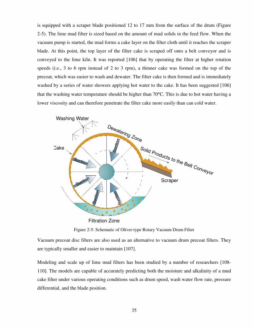
35

is equipped with a scraper blade positioned 12 to 17 mm from the surface of the drum (Figure

2-5). The lime mud filter is sized based on the amount of mud solids in the feed flow. When the

vacuum pump is started, the mud forms a cake layer on the filter cloth until it reaches the scraper

blade. At this point, the top layer of the filter cake is scraped off onto a belt conveyor and is

conveyed to the lime kiln. It was reported [106] that by operating the filter at higher rotation

speeds (i.e., 3 to 6 rpm instead of 2 to 3 rpm), a thinner cake was formed on the top of the

precoat, which was easier to wash and dewater. The filter cake is then formed and is immediately

washed by a series of water showers applying hot water to the cake. It has been suggested [106]

that the washing water temperature should be higher than 70°C. This is due to hot water having a

lower viscosity and can therefore penetrate the filter cake more easily than can cold water.

Figure 2-5: Schematic of Oliver-type Rotary Vacuum Drum Filter

Vacuum precoat disc filters are also used as an alternative to vacuum drum precoat filters. They

are typically smaller and easier to maintain [107].

Modeling and scale up of lime mud filters has been studied by a number of researchers [108-

110]. The models are capable of accurately predicting both the moisture and alkalinity of a mud

cake filter under various operating conditions such as drum speed, wash water flow rate, pressure

differential, and the blade position.

Cake

Washing Water

Scraper

Filtration Zone

36

2.7 Summary

There are several studies to relate lime mud characteristics to filtration and dewatering

behaviours. Although these studies made important contributions to the understanding of lime

mud dewatering, the mechanisms that prevent lime mud from settling and filtering easily are not

well understood.

Since the liming ratio has a significant impact on the settling rate and filterability of lime mud,

and hence, on the thermal efficiency of the lime kiln, the focus of the present thesis is to

systematically investigate the effect of liming ratio on the causticizing efficiency (CE), physical

characteristics (particle size distribution, zeta potential, etc.), settling rate, and filterability of the

precipitated lime muds.

Furthermore, despite the fact that there exist a few experimental studies on overliming, there has

been no reliable method for measuring the degree of overliming directly in the causticizing plant.

In kraft mills, an overliming condition is noticed only when the lime mud does not settle well

and/or when the filterability is poor.

37

3 Experimental Techniques

3.1 Slaking and Causticizing Reactions

Figure 3-1 shows the experimental setup used in this study. A tightly sealed jar containing 300

ml of Na2CO3 solution was placed in a water bath controlled at 95°C (± 1°C). The liquid

temperature inside of the reaction vessel was monitored using a thermocouple inserted directly

into the solution through a threaded hole. The liquid temperature inside the vessel was 88°C (±

2°C) prior to lime addition. Lime was poured quickly into the jar and the slurry was constantly

agitated with a motorized stirrer for 90 minutes to allow the slaking and causticizing reactions

(as described in Section 1.1) to proceed to completion. Depending on the test conditions, the

liming ratio (i.e., molar ratio of CaO to Na2CO3) in the feed was varied. The lime quantity was

calculated based on the moles of Na2CO3 per liter of water.

Figure 3-1: Schematic of the Slaking and Causticizing Vessel

The reburned lime samples used in this study were collected from four kraft pulp mills at the

outlet of the lime crusher at the discharge end of the kiln. The samples were calcined again in a

laboratory muffle furnace at 900 ºC for 60 minutes to ensure that they were fully calcined. The

samples were stored in airtight bags with only a small portion of each used for testing.

38

In addition to the reburned lime, pure lime (analytical grade with 99.9 wt. % CaO purchased

from Fisher Scientific Canada) was also used. Synthetic green liquor with a TTA (Total

Titratable Alkali) value of 120 g/L Na2O was prepared by dissolving analytical grade Na2CO3

(with 99.5 wt. % Na2CO3 purchased from Fisher Scientific Canada) in distilled water.

To produce Ca(OH)2, 300 mL of distilled water was kept at 95 ºC (±1 ºC) in a hot water bath. A

known weight of reburned lime was poured quickly into the jar and the slurry was kept

suspended by a motorized stirrer for 90 minutes, which allowed the slaking reaction to proceed

to completion.

After the slaking and causticizing reactions, 100 mL of slurry from the reaction vessel was

poured onto a filter paper in a funnel placed on a flask, and vacuum-filtered. The filtered solution

(filtrate) was stored in an airtight bottle until it was analyzed for NaOH and Na2CO3 by titration.

The titration analysis results were used to calculate the causticizing efficiency (CE). The wet

cake (solids) on the filter paper after filtration was washed with methanol to reduce the surface

tension of water between particles, and then washed with boiling deionized water to remove any

residual alkali. The washed cake was weighed and dried in a vacuum oven at 90 °C for 24 hours

before undergoing physical and chemical analyses.

3.2 Settling

After slaking and causticizing, 100 mL of the well-mixed slurry was transferred to a graduated

cylinder immersed in a water bath maintained at 95 °C for a batch settling test (Figure 3-2). A

graduated glass cylinder 24.5 cm in height and with a 2.61 cm inner diameter (ID) was selected

for the settling tests. It was chosen this size of graduated cylinder because we found using larger

ID cylinders (5.95 cm ID) obtained the same results (see Appendix B).

The cylinder was covered with a glass disc to minimize the carbonation of Ca(OH)2 by CO2

present in the air. The suspension was allowed to settle, and the change in the height of the

interface between supernatant (the clear liquid portion) and the sediment (cloudy liquid-particles

portion) in the cylinder was monitored with time. The settling curve was constructed by

measuring the height of the interface every 2 minutes for the first 30 minutes, and every 5

minutes thereafter, until the interface came to rest. The cylinder was then withdrawn from the

39

water bath and tapped gently before the final reading was recorded. The settling velocities were

calculated from the initial slope of the settling curves.

Figure 3-2: Settling Test Set-up

3.2.1 Five-Minute Settling Test

A common test to determine the overliming condition in the causticizing plant of a kraft pulp

mill is the “5-minute settling test” [21].

In this test, the mill operator places 1 L of the causticizer slurry (white liquor with precipitated

lime mud) in a cone shaped cylinder. Samples are taken from the process after the slaker and

causticizer vessels. Then the slurry is allowed to settle and a change in the height of the interface

between supernatant (the clear liquid portion) and the sediment (cloudy liquid-particles portion)

in the cylinder is measured after 5 minutes. If solids settle to between 50 % and 60 % of the total

volume in 5 minutes and the liquor above solids is clear, the operator concludes that the system

is not overlimed. If the slurry settles slowly and/or the liquor is cloudy, it is then assumed that

the system is overlimed and free lime is present.

Thermometer

Water Bath

(95°C)

Sample

Thermometer

Water Bath

(95°C)

Sample

40

3.3 Filterability

3.3.1 Original Set-up

A common test to evaluate the filtration characteristics of a rotary vacuum filter is a vacuum leaf

test, undertaken at constant pressure or vacuum [111].

After the slaking and causticizing reactions, 100 mL of slurry was poured onto a vacuum

filtration apparatus as shown in Figure 3-3. The apparatus consisted of a 4.7 cm diameter filter

holder with a 250 ml graduated reservoir. The base of the filter holder was a perforated plate

with a filter paper placed on top. A Whatman No. 4 filter paper was used in the filtration and

dewatering tests. Vacuum was applied to the graduated cylinder (filtrate container) using a rotary

vacuum pump. The filtration was carried out at a constant vacuum of 14 kPa. The vacuum level

was monitored using a pressure gauge and was regulated using a by-pass valve on the pump. The

volume of the filtrate (V) collected in the graduated cylinder was measured over a fixed length of

time (t). After all the water had passed through the solids cake, the dewatering was continued for

an additional 30 seconds. The cake was then removed, weighed and dried in an oven at 110 °C

for 24 hours. The moisture content of the cake was determined (in accordance with TAPPI

Standard for moisture content analysis of pulp – T412om-06 [112]), using Equation (24):

Figure 3-3: Bench Scale Dewatering Equipment Set-up

Funnel

Pressure

Gauge

Graduated

Cylinder

Slurry

Vacuum

Pump

Perforated Plate

41

100m

mmContentMoisture

0

10 ×−

= (24)

where m0 and m1 are the weight of the cake before and after drying in an oven, respectively.

The average specific resistance αav and the medium resistance Rm were calculated by plotting t/V

against V and drawing a line of best fit through the data using Equation (11) as discussed in

Section 2.2.

3.3.2 Modified Set-up

To avoid filter clogging and to improve the reliability of measurements, the experimental set-up

was modified. As shown in Figure 3-4, in the modified set-up the slurry was fed into a sealed

container and a vacuum was applied across a filter. The apparatus consisted of a 5.5 cm diameter

filter holder mounted on a sealed jar and connected by coiled tubing to a filtrate vessel placed on

an electronic balance with a data acquisition system. The filter holder was fitted with a Whatman

No. 4 filter paper. For each test, a known weight of a dried lime mud sample produced from the

causticizing reaction was used. The sample was dried in a vacuum oven after filtration as

described in Section 3.1, and was mixed with 100 mL of de-ionized water to obtain a mud slurry

of 20% solids by weight. Vacuum was applied to the filtrate vessel using a rotary vacuum pump.

The tests were conducted at a constant pressure of 65 kPa. In this set-up applied pressure is

higher than in the original set-up to support building a thick filter cake. The applied pressure

should overcome the increasing weight of the filter cake and the higher pressure loss of the line.

The vacuum level was measured using a digital manometer and regulated using a by-pass valve

on the pump. The weight of the filtrate collected was measured over a fixed length of time (t = 3

minutes). The cake was weighed and dried in an oven at 110 °C for 24 hours. The moisture

content of the cake was determined based on the loss in weight on drying.

42

Figure 3-4: Filterability Test Set-up

3.4 Titration

CO32-

and OH-

concentrations were determined by titration of samples with a 1.0 N

hydrocholoric acid (HCl) solution (in accordance with TAPPI Standard for white liquor (NaOH)

analysis – T624os-68 [113]). The titration was conducted with an automatic titration device

Metrohm 751 GPD Titrino.

A titration curve was displayed by the titration device which automatically calculated both the

volume of HCl added to the sample and the pH value of each equivalent. The amount of

hydroxide and carbonate in the sample was calculated based on the volume of HCl added to

reach the first and third equivalent points, respectively. Causticizing efficiency (CE %) of the

reaction was determined using Equation (19) presented in Section 2.6.1.1.

3.5 Particle Size Distribution (PSD)

The particle size distribution measurements were carried out using Malvern’s Mastersizer S laser

particle size analyzer. The device employs a laser for light scattering diffraction analysis to

obtain a particle size distribution. The detection range of the instrument is from 0.05 to 3500 µm

[114]. The value of the refractive index was 1.33. The suspensions were prepared using

distillated water in order to have well dispersed and homogeneous samples at an appropriate

concentration (15-20 % obscuration).

Magnetic Stirrer

To Vacuum Pump

Balance

VentVent

Filter Holder

Filtrate

Data Acquisition

Pressure Gauge

Filter Cake

43

Some particle size distribution measurements were also performed by a Microtrac S3500 laser

particle size analyzer with a detection range of 0.02 to 2816 µm.

3.6 Surface Area of Particle

The surface area of the lime particles were measured by the Brunauer-Emmett-Teller (BET)

method using an Autosorb-1 (Quantachrome, US) BET set-up with N2 as adsorbate. The N2

physisorption isotherm was measured and plotted as Vgas vs. P/P0. Using the adsorption isotherm,

the equipment determines the volume of gas required to form a film of adsorbed molecules (i.e.,

a monolayer) on the solid surface. The volume-pressure data can be reduced by the

AUTOSORB-1 software into BET surface area in a range of 0.1-0.35 P/P0 on the isotherm using

an extensive set of built-in data-reduction procedures.

3.7 Zeta Potential

Zeta potential (ζ) measurements were performed by the micro-electrophoretic apparatus Zeta

Plus (Brookhaven Instruments Corporation, U.S.A). This instrument determines the

electrophoretic mobility and converts to ζ using Smoluchowski’s model. The suspensions were

made by adding 0.1 g of mud particles to 500 mL of distilled water at 23 °C ± 1. The pH was

adjusted to 10.5 ± 0.2 using white liquor produced by the causticizing reactions.

As illustrated in Figure 3-5, the measurement of ζ employs laser light-scattering and comparison

to a reference beam. The laser beam passes through the sample in the sample cell holder, which

carries two electrodes to induce the electric field. The light which is scattered by the particles is

Doppler shifted because the scattering particles are moving in the electric field. This scattered

beam is mixed with the reference beam at the detector (photo-multiplier-tube (PMT)). The

reference beam is modulated and a frequency shift is used to calculate both the sign and

magnitude of the electrophoretic mobility.

44

Figure 3-5: Zeta Plus Optics Apparatus

3.8 Thermal Gravimetric Analysis

Mud samples were tested for Ca(OH)2 contents using a simultaneous thermogravimetric

Analysis (TGA) and differential thermal analysis (DTA) instrument, Model SDT Q600TM

from

TA Instrument.

Mud samples, approximately 20 mg each, were placed in the aluminum sample pan, and the

changes in sample weight were recorded as a function of temperature as samples were heated

over the temperature range 25-910 °C at a scanning rate of 20 °C/min in nitrogen, which was

passed through the TGA/DSC instrument at 100 mL/min. The Ca(OH)2 content was calculated

based on the weight loss between 300 and 500 °C where the decomposition of calcium hydroxide

to calcium oxide occurs, while the CaCO3 content in the mud was calculated from the weight

loss between 600 and 900 °C where the decomposition of calcium carbonate to calcium oxide

occurs.

3.9 Scanning Electron Microscopy

Scanning electronic microscopy (SEM) images were obtained using a JEOL JSM-840 scanning

electron microscope to study the morphology and state of aggregation of CaCO3 particles. Mud

samples were coated with gold prior to testing to enable charge removal during SEM operation.

45

3.10 Atomic Absorption Spectroscopy (AAS)

Sodium and calcium concentrations were analyzed using atomic absorption (AA) spectroscopy.

The spectrometer used was a Varian Spectra AA-250 Plus. White liquor samples were diluted in

deionized water to produce solutions containing 1 to 50 ppm Ca2+

and 1 to 10 ppm Na+. In this

technique, the sample solution is aspirated into an air-acetylene flame, and the elemental Na or

Ca is converted to an atomic vapor [115]. Most atoms of the test element remain in the ground

state and can absorb radiation of a particular wavelength specific to that element. The

wavelengths of the radiation given off by the source of the radiation are the same as those

absorbed by the atoms in the flame. Hence, the absorbance is directly proportional to the path

length in the flame and to the concentration of atomic vapor in the flame. Since the path length

can be kept constant, the concentration of the element in the solution can directly be determined.

Atomic absorption (AA) spectroscopy results for white liquor produced from pure lime, R-Lime

“A” and R-Lime “B” samples are presented in Appendix C.

3.11 X-ray Florescence Spectroscopy (XRF)

The elemental composition of the reburned lime samples were determined using an x-ray

florescence spectroscope (Philips PW2404). The equipment gives qualitative and quantitative

information on the elements that may be present in the samples using a semi-quantitative

software package and custom calibration with the selected method.

3.12 X-Ray Diffraction Analysis (XRD)

X-ray diffraction patterns of the samples were obtained with a Philips PW3710 diffractometer

utilizing Cu Ka radiation in the range 15–60° 2θ with a step size of 0.02°. The acquisition time

was measured at 2.5 s per step. The generated patterns were compared with the International

Centre for Diffraction Data® files to identify the crystallographic structure of the samples.

3.13 OLI, Advanced Simulation Software

To study the thermodynamic stability of different Ca species in an aqueous solution, a relative

distribution diagram (stability diagram) of Ca species was constructed using OLI Stream

46

AnalyzerTM

version 2.0. The program is capable of predicting the phases as well as the chemical

reaction behaviour, based on the equilibrium state equations for the reaction and species

involved.

47

4 Experimental Results and Discussion

The settling and filterability of lime mud are closely related. Mill experience says that lime mud

with a slower settling rate tends to be more difficult to filter and less adept at cake formation.

Although, in this thesis, the effect of various parameters on lime mud dewatering was evaluated

based on data obtained mainly from settling rate, data from lime mud filterability tests were also

used to support the conclusions wherever possible.

This chapter contains six sections. As noted in previous chapters, liming ratio has a significant

impact on the settling rate and filterability. The reburned lime samples used were characterized

in Section 4.1. The effect of liming ratio on the settling was investigated in Section 4.2. To study

the effect of liming ratio, settling velocities and solid fluxes were calculated from settling data

for lime muds prepared by causticizing a pure Na2CO3 solution with pure CaO and/or reburned

lime B. The results and related discussion are presented in Section 4.2.1. Increasing the solids

content increases the potential for particle-particle interactions. This, in turn, can influence the

settling rate of lime mud. The effect of solids content is studied in Section 4.2.2. The effect of

lime type on settling is investigated in Section 4.2.3.

Section 4.3 reviews the impact of liming ratio, solids content, and lime type on filterability.

Filterability test data were used to determine specific cake and medium resistance by plotting t/V

(time required to filter a V volume of filtrate) against V (filtrate volume).

The causticizing efficiency is an important parameter in the kraft process. Section 4.4 studies the

impact of liming ratio on the causticizing efficiency. The test results were used to show the

adverse effect of overliming on the settling and filterability without improvement to the

causticizing efficiency beyond a certain extent.

Section 4.5 investigates the effect of liming ratio on the mud particle size and shape. Different

analytical techniques were used to investigate the physical features of lime mud particles.

As noted in Chapter 2, it is a common belief that overliming promotes generation of small size

Ca(OH)2 particles from the causticizing reaction and that these fine particles are the main cause

of settling and filterability difficulties. Section 4.6 evaluates the validity of this hypothesis.

48

Particle charge has a significant effect on settling and filterability. Section 4.7 discusses the

effect of liming ratio on the zeta potential (ζ) of lime mud particles. The results were used to

establish a correlation between changes in particle charge and free lime content of lime mud

particles when the system state changed from underliming to overliming.

The causticizing reaction conditions were kept constant at 120 g/L Na2O TTA, and 90 minutes

throughout this work.

4.1 Reburned Lime Characteristics

The reburned lime samples used in this study were identified as R-Lime “A”, R-Lime “B”, R-

Lime “C”, and R-Lime “D” respectively from mills A, B, C, and D. Table 4-1 summarizes the

chemical composition and physical properties of the samples. The composition, expressed as

oxides, was determined by means of x-ray fluorescence spectroscopy (XRF). A scanning

electron microscope (SEM) was also used to examine the morphology of the lime particles.

Figure 4-1 shows that the reburned lime samples mainly consist of agglomerates of large

crystals. The agglomerates have different shapes. The cumulative particle size distribution of

samples was determined using a Malvern Mastersizer S laser particle size analyzer. Mean

particle sizes estimated from these data are presented in Table 4-1.

49

Figure 4-1: SEM of Reburned Limes, a) Mill A, b) Mill B, c) Mill C, d) Mill D, and e) Pure CaO

50

Table 4-1: Physical and Chemical Characteristics of Reburned Limes

Item Unit R-Lime

“A”

R-Lime

“B”

R-Lime

“C”

R-Lime

“D”

Mean number diameter µm 7.4 30.9 14.2 10.3

Specific Surface Area4 m

2/g 0.8 0.3 0.4 0.6

Zeta Potential mV +36.6 +32.2 +34.3 +31.6

Composition5

CaO

wt. %

88.1 91.7 86.2 89.3

MgO 5.5 4.3 1.9 2.6

Na2O 1.4 0.7 1.5 1.4

P2O5 1.5 1.6 2.5 2.0

MnO 0.9 0.01 n/a 0.02

SO3 0.7 1.0 0.9 1.5

Fe2O3 0.5 0.1 n/a 0.1

Si2O 0.2 0.3 0.4 0.4

Al2O3 0.2 0.1 0.3 0.1

Other 0.8 0.2 6.3 2.6

4.2 Lime Mud Settling

4.2.1 Liming Ratio

Figure 4-2 shows pictures of a mixture with a liming ratio of 0.6 at different times of settling.

Time zero (t = 0) represents the start of the settling right after the slurry was poured into the

graduated cylinder. This series of pictures shows the progression of the settling and the descent

of the interface with time.

4 Determined by the gas adsorption technique (BET)

5 Determined by X-Ray Fluorescence Spectroscopy (XRF)

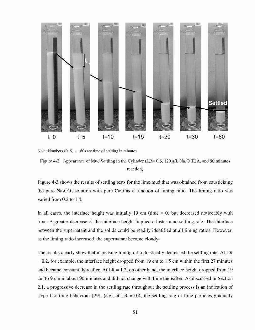
51

Note: Numbers (0, 5, …, 60) are time of settling in minutes

Figure 4-2: Appearance of Mud Settling in the Cylinder (LR= 0.6, 120 g/L Na2O TTA, and 90 minutes

reaction)

Figure 4-3 shows the results of settling tests for the lime mud that was obtained from causticizing

the pure Na2CO3 solution with pure CaO as a function of liming ratio. The liming ratio was

varied from 0.2 to 1.4.

In all cases, the interface height was initially 19 cm (time = 0) but decreased noticeably with

time. A greater decrease of the interface height implied a faster mud settling rate. The interface

between the supernatant and the solids could be readily identified at all liming ratios. However,

as the liming ratio increased, the supernatant became cloudy.

The results clearly show that increasing liming ratio drastically decreased the settling rate. At LR

= 0.2, for example, the interface height dropped from 19 cm to 1.5 cm within the first 27 minutes

and became constant thereafter. At LR = 1.2, on other hand, the interface height dropped from 19

cm to 9 cm in about 90 minutes and did not change with time thereafter. As discussed in Section

2.1, a progressive decrease in the settling rate throughout the settling process is an indication of

Type I settling behaviour [29], (e.g., at LR = 0.4, the settling rate of lime particles gradually

t=0 t=5 t=10 t=15 t=20 t=30 t=60

Settled

U0

52

decreased with time from 19 cm to 3 cm). The results suggest that for tests with low liming

ratios, the resulting lime mud follows Type I settling behaviour.

Figure 4-3: Effect of Liming Ratio on Settling Curve (120 g/L Na2O TTA, and 90 minutes reaction), Pure

CaO

At higher liming ratios, for example LR = 1, the interface height became constant at 8 cm after

60 minutes, while at LR = 1.4, it decreased at a much slower rate and became constant only after

110 minutes. For these conditions, it is possible to have a very short induction period in which

loosely aggregated particles were formed and no sedimentation occurred. This was followed by a

constant decrease in the interface height, exhibiting the zone settling regime. A steady-state

compression settling subsequently took place with a much lower rate. As the liming ratio is

increased, the length of the initial induction is increased, suggesting a Type II settling behaviour,

which slows the settling of the mud particles.

To study the effect of liming ratio on settling rates, the settling velocities were calculated as the

initial slope of the settling curves. Figure 4-4 shows the effect of liming ratio on the settling

velocity for pure lime on logarithmic scale. The results indicate that increasing liming ratio from

0

5

10

15

20

0 20 40 60 80 100 120

Time, min

Inte

rfa

ce

He

igh

t, c

m

0.2

0.4

0.60.8

1

[CaO]/[Na2CO3]=1.4

1.2

53

0.2 to 1.4 decreased the settling velocity from 2.7 cm/min to 0.09 cm/min, respectively. They

also show two different slopes of settling rate. The changes in the slope of settling rate plots

suggest changes in the settling mechanisms. At higher liming ratios, however, the average

settling rate becomes much lower. For example, increasing the liming ratio from 0.2 to 0.6

decreased the average settling rate from 2.7 cm/min to 0.3 cm/min, while increasing liming ratio

from 0.6 to 1.4 decreased the average settling rate from 0.3 cm/min to 0.09 cm/min.

Figure 4-4: Settling Velocity as a Function of Lime Dosage (120 g/L Na2O TTA, and 90 minutes

reaction), Pure CaO

0.01

0.10

1.00

10.00

0 0.2 0.4 0.6 0.8 1 1.2 1.4

Se

ttli

ng

Ve

loc

ity,

cm

/min

[CaO]/[Na2CO3]

10

1

0.1

54

The above clearly demonstrates strong dependence of the settling rate on liming ratio. To make

sure that the above results are not only for the lime mud produced by causticizing pure Na2CO3

solution with pure CaO, experiments were also carried out on lime mud obtained by causticizing

the pure Na2CO3 solution with R-Lime “B” at different liming ratios. The results are shown in

Figure 4-5. Similar to the behaviour of lime mud produced from pure chemicals, the settling rate

decreased considerably with an increase in liming ratio. At LR = 0.18, the lime mud obtained

appeared to be coarse and sandy. It settled rapidly to the bottom of the cylinder with a turbid

supernatant. As the liming ratio increased, the supernatant turbidity decreased. At higher liming

ratios, for example 0.92, the length of the initial induction increased, the settling occurred with a

much lower rate, and the interface height became constant at 7 cm after 35 minutes, while at 1.3,

the interface height decreased at a much slower rate and became constant after 50 minutes.

Consistent with the first set of tests, with increasing liming ratio settling behavior changed from

Type I to Type II.

Figure 4-5: Effect of Liming Ratio on Settling Curve (120 g/L Na2O TTA, and 90 minutes reaction), R-

Lime “B”

The results of the settling tests for reburned limes from Mills A, C, and D are presented in

Appendix D. For all samples, the results clearly show that increasing the liming ratio considerably

decreased the settling rate. The mud sample settling tests also show similar behaviours as a

function of increasing liming ratios.

0

5

10

15

20

0 10 20 30 40 50 60 70 80

He

igh

t o

f In

terf

ac

e,

cm

Time, min

0.92

0.55

0.73

1.1

[CaO]/[Na2CO3]=1.3

0.380.18

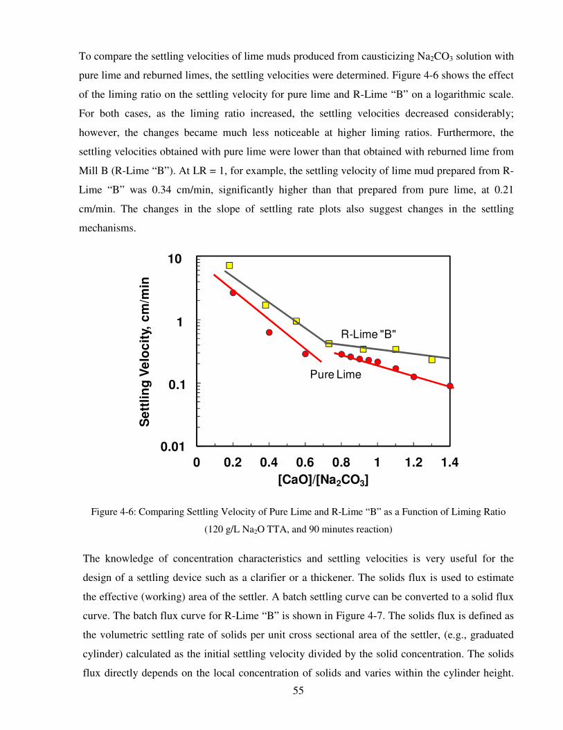
55

To compare the settling velocities of lime muds produced from causticizing Na2CO3 solution with

pure lime and reburned limes, the settling velocities were determined. Figure 4-6 shows the effect

of the liming ratio on the settling velocity for pure lime and R-Lime “B” on a logarithmic scale.

For both cases, as the liming ratio increased, the settling velocities decreased considerably;

however, the changes became much less noticeable at higher liming ratios. Furthermore, the

settling velocities obtained with pure lime were lower than that obtained with reburned lime from

Mill B (R-Lime “B”). At LR = 1, for example, the settling velocity of lime mud prepared from R-

Lime “B” was 0.34 cm/min, significantly higher than that prepared from pure lime, at 0.21

cm/min. The changes in the slope of settling rate plots also suggest changes in the settling

mechanisms.

Figure 4-6: Comparing Settling Velocity of Pure Lime and R-Lime “B” as a Function of Liming Ratio

(120 g/L Na2O TTA, and 90 minutes reaction)

The knowledge of concentration characteristics and settling velocities is very useful for the

design of a settling device such as a clarifier or a thickener. The solids flux is used to estimate

the effective (working) area of the settler. A batch settling curve can be converted to a solid flux

curve. The batch flux curve for R-Lime “B” is shown in Figure 4-7. The solids flux is defined as

the volumetric settling rate of solids per unit cross sectional area of the settler, (e.g., graduated

cylinder) calculated as the initial settling velocity divided by the solid concentration. The solids

flux directly depends on the local concentration of solids and varies within the cylinder height.

0.01

0.10

1.00

10.00

0 0.2 0.4 0.6 0.8 1 1.2 1.4

Se

ttli

ng

Ve

loc

ity,

cm

/min

[CaO]/[Na2CO3]

R-Lime "B"

Pure Lime

10

1

0.1

56

As the concentration of solids increases with depth and the amount of liquid that is displaced

(upward) by the solids decreases, upward drag on the particles changes.

As the results indicate, a batch flux curve features a maximum and a minimum, and this can be

explained by considering two limits: at zero concentration the flux must be zero, and at the

highest possible concentration the flux will be again zero because the settling velocity term will

reach zero. Between these two extremes the flux has finite values since the settling velocity is

nearly constant in the free settling region. Hence, the batch flux curve exhibits a maximum at a

low liming ratio, as illustrated in Figure 4-7. The solid flux first decreases sharply and then

decreases gradually with increasing liming ratio. The initial sharp decrease is due to Type I

settling of a dilute slurry, the subsequent decrease is attributed to the settling behavior changing

from Type I to Type II settling.

Figure 4-7: The Batch Flux Curve as a Function of Lime Ratio (120 g/L Na2O TTA, and 90 minutes

reaction), R-Lime “B”

0

10

20

30

0 10 20 30 40

So

lid

Flu

x,

g/c

m2.m

in

Solids Concentration, g/cm3

Experimental Data

57

Figure 4-8 plots the final interface height as a function of liming ratio for lime muds produced

from causticizing Na2CO3 solution with R-lime “B”. As shown, the final interface height

increased non-linearly with an increase in the liming ratio suggesting that an increase in the

liming ratio proportionally increases the solids content of the slurry.

Figure 4-8: Relationship between Liming Ratio and Final Interface Height shown in Figure 4-5

To summarize, this section utilized different techniques and approaches to investigate the effect

of the liming ratio on the settling rate. As shown in Figure 4-3 and Figure 4-5 and supported by

other results, increasing the liming ratio results in a lower settling rate, although it is not clear

that the slower settling is only related to the liming ratio or also to the higher solids content and

higher potential for particle-particle interactions. At higher particle concentrations, particles are

closer to one another; their movements inevitably interfere with one another. With an increase in

particle concentration, the free area between particles is reduced, causing interparticle fluid

velocities and alteration of flow patterns around particles [26].

4.2.2 Effect of Solids Content

To investigate the effect of solids content on the settling behaviour, a series of lime mud slurries

with different solids content ranging from 5 wt. % to 25 wt. % were prepared. To prepare these

samples, a known weight of dried lime mud that was obtained from causticizing pure Na2CO3

0

2

4

6

8

10

12

0 0.2 0.4 0.6 0.8 1 1.2 1.4

Fin

al In

terf

ac

e H

eig

ht,

cm

[CaO]/[Na2CO3]

58

solution with R-Lime “B” at LR = 1, was mixed with 25 mL of deionized water to obtain the

targeted slurry concentration. The samples were allowed to stand for 24 hours before being

transferred to a graduated cylinder for the settling test.

Figure 4-9 shows the effect of slurry concentration on the settling rate of lime mud (R-Lime “B”)

at LR = 1. As expected, the settling velocity of particles decreased steadily as the concentration

of the suspension increased. For higher concentrations, the rate of particle settling was lower due

presumably to greater upward velocity of the displaced fluid [116].

Figure 4-9: Effect of Solids Content on Settling Curve (R-Lime “B”, [CaO]/ [Na2CO3] =1,

120 g/L Na2O TTA, and 90 minutes reaction)

0

2

4

6

8

10

12

14

0 10 20 30 40 50 60 70

Inte

rface H

eig

ht,

cm

Time, min

Solids Content

20 %

15 %

5 %

10 %

25 %

59

Figure 4-10 shows particle settling velocities plotted against solids content. As shown,

increasing the solids content from 5 wt. % to 25 wt. % decreased the settling velocity

considerably from 2.25 cm/min to 0.34 cm/min. Increasing the concentration of particles

suspended in a fluid increases the density and viscosity of the suspension. As a particle falls it

must displace a volume of fluid equal to its own. Consequently, the apparent settling velocity of

the particles in the concentrated suspensions is less than of that of a discrete particle of similar

properties (e.g., the same liming ratio). This further confirms the adverse effect of solids content

on the settling rate.

Figure 4-10: Effect of Solids Concentration on Settling Velocity (R-Lime “B”, [CaO]/

[Na2CO3] =1, 120 g/L Na2O TTA, and 90 minutes reaction)

To investigate the effect of particle-particle interactions on settling, additional settling tests were

carried out at various liming ratios with constant solids content. In such tests, a known weight of

dried lime mud that was obtained from causticizing pure Na2CO3 solution with R-Lime “B” with

liming ratios ranging from 0.38 to 1.3 were mixed with 25 mL of deionized water to obtain mud

slurries of 6 wt. % solids. Figure 4-11 shows the results of these tests. In this case, since solids

content was the same for all tests at different liming ratios, the height of the interface settled at

the same final level of 1.8 cm. The results clearly suggest that the higher liming ratio was the

main cause of slower mud settling.

0

0.5

1

1.5

2

2.5

0 10 20 30

Se

ttli

ng

Ve

loc

ity,

cm

/min

Solids Concentration, %

60

Figure 4-11: Effect of Liming Ratio on Settling Curve of Mud Produced from Mill B Reburned

Lime at a Constant Slurry Concentration of 6 wt. % (120 g/L Na2O TTA, and 90 minutes

reaction)

Figure 4-12 presents the settling of the mud produced from Mill B (R-Lime “B”) reburned lime

at a constant slurry concentration of 20 wt. % as a function of liming ratio. Similar to the tests at

6 wt. % slurry concentration, the settling rate decreased with an increase in the liming ratio. At a

given liming ratio, however, the settling rate was slower at a higher solids concentration. For

example at LR = 0.92, increasing the solids content from 6 wt. % to 20 wt. % decreases the

settling velocity from 1.5 cm/min to 0.23 cm/min.

The above confirms that although the solids content noticeably influences the settling, it is not

the only cause of the decrease in the settling rate. The liming ratio has a significant impact on the

settling rates as well.

0

2

4

6

8

10

12

14

0 15 30

Inte

rface H

eig

ht,

cm

Time, min

0.92

0.73

[CaO]/[Na2CO3]

1.1

1.3

0.38

61

Figure 4-12: Effect of Liming Ratio on Settling Curve of Mud Produced from Mill B Lime at a Constant

Slurry Concentration of 20 wt. % (120 g/L Na2O TTA, and 90 minutes reaction)

4.2.3 Lime Type

To investigate the effect of lime type on the settling rate, a series of experiments were conducted

to test the settling rates of different limes at a constant liming ratio. Figure 4-13 compares

settling rates of lime muds produced from causticizing pure Na2CO3 solution with different

reburned limes and pure CaO at LR = 1. The settling rates were noticeably different depending

on the lime type used. At the same liming ratio, however, reburned limes produced lime muds

that were easier to settle.

As shown in Figure 4-14, although the initial solids content was the same, different lime types

did not give the same final interface height. The results imply that the final sedimentation height

may be related to the porosity of the sediment, which in turn, depends on the amount of

entrapped water as well as the strength of the attractive forces between flocs [51].

0

2

4

6

8

10

12

14

0 10 20 30 40 50 60

Inte

rfa

ce

He

igh

t, c

m

Time, min

0.550.92

[CaO]/[Na2CO3]

0.73

1.11.3

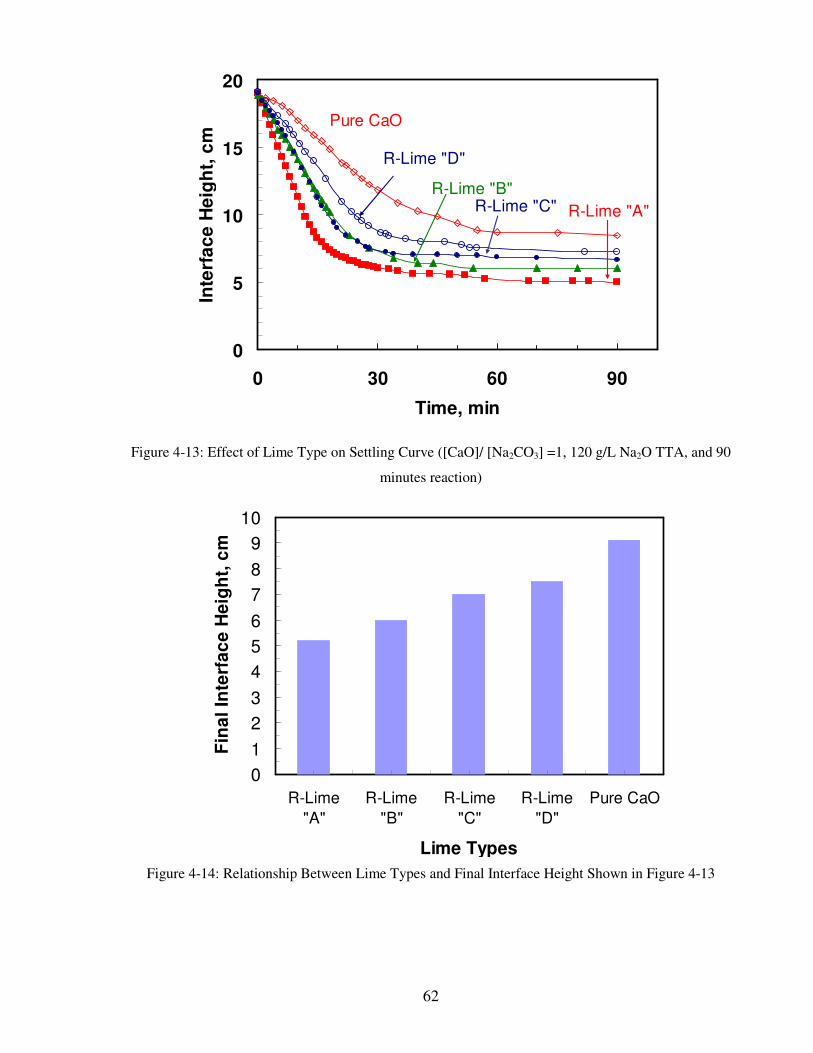
62

Figure 4-13: Effect of Lime Type on Settling Curve ([CaO]/ [Na2CO3] =1, 120 g/L Na2O TTA, and 90

minutes reaction)

Figure 4-14: Relationship Between Lime Types and Final Interface Height Shown in Figure 4-13

0

5

10

15

20

0 30 60 90

Time, min

Inte

rfa

ce

He

igh

t, c

m

Pure CaO

R-Lime "A"

R-Lime "B" R-Lime "C"

R-Lime "D"

0

1

2

3

4

5

6

7

8

9

10

R-Lime

"A"

R-Lime

"B"

R-Lime

"C"

R-Lime

"D"

Pure CaO

Lime Types

Fin

al

Inte

rfa

ce

He

igh

t, c

m

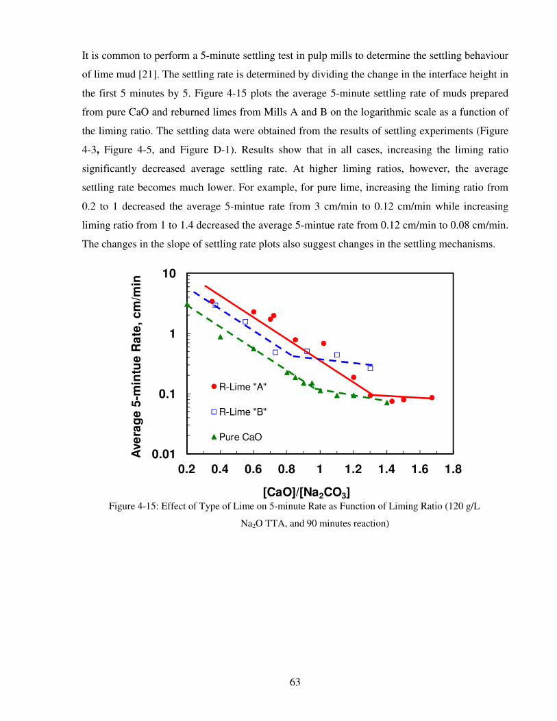
63

It is common to perform a 5-minute settling test in pulp mills to determine the settling behaviour

of lime mud [21]. The settling rate is determined by dividing the change in the interface height in

the first 5 minutes by 5. Figure 4-15 plots the average 5-minute settling rate of muds prepared

from pure CaO and reburned limes from Mills A and B on the logarithmic scale as a function of

the liming ratio. The settling data were obtained from the results of settling experiments (Figure

4-3, Figure 4-5, and Figure D-1). Results show that in all cases, increasing the liming ratio

significantly decreased average settling rate. At higher liming ratios, however, the average

settling rate becomes much lower. For example, for pure lime, increasing the liming ratio from

0.2 to 1 decreased the average 5-mintue rate from 3 cm/min to 0.12 cm/min while increasing

liming ratio from 1 to 1.4 decreased the average 5-mintue rate from 0.12 cm/min to 0.08 cm/min.

The changes in the slope of settling rate plots also suggest changes in the settling mechanisms.

Figure 4-15: Effect of Type of Lime on 5-minute Rate as Function of Liming Ratio (120 g/L

Na2O TTA, and 90 minutes reaction)

0.01

0.1

1

10

0.2 0.4 0.6 0.8 1 1.2 1.4 1.6 1.8

Ave

rag

e 5

-min

tue

Ra

te,

cm

/min

[CaO]/[Na2CO3]

R-Lime "A"

R-Lime "B"

Pure CaO

64

4.3 Lime Mud Filterability

4.3.1 Liming Ratio

Using the test set-up described in Section 3.2.1, the effect of liming ratio on lime mud

filterability was studied. Figure 4-16 shows the filterability represented as t/V (time required to

filter a V volume of filtrate) for the lime muds obtained using R-Lime “B” as a function of slurry

volume and liming ratio. The liming ratio was varied from 0.18 to 1.3. Since the filtration of fine

particles in a suspension is dependent on pH and temperature, filtration tests were performed at

ambient temperature and a pH of 10.5.

It should be noted that non-linearity in the plot of the (t/V, V) data can often be seen close to the

start and end of the filtration. The non-linearity in the beginning of the tests is likely due to

changes in the cake thickness. In the initial stage of the filtration when the cake is very thin, the

main part of the total pressure drop is over the filter medium. As the cake becomes thicker, the

pressure drop becomes across the cake and cake resistance dominates the medium resistance.

The non-linearity at the end of the filtration is caused by particulates at high liming ratios, and it

may be due to the decrease in flow rate from thick cake formation, which significantly reduces

the filtrate flow rate.

65

Figure 4-16: t/V vs. V Plots as Function of Liming Ratio (120 g/L Na2O TTA, 90 minutes

reaction, and 14 KPa Vacuum), R-Lime “B” using Filterability Set-up as Shown in

Figure 3-3

Figure 4-16 shows that at LR = 0.18, for example, the filtration finished more quickly than in the

higher LRs, and most filtrate (liquid) was released in a short time period (i.e., after one minute

of filtration). The samples with high liming ratios (i.e., LR = 1.3), on the other hand, finished

more slowly, and filtrate drained out continuously through the entire filtration period (seventeen

minutes of filtration). The results clearly indicate that increasing liming ratio considerably

decreases the filterability. The slope of fitted lines to data points increases with an increase in

slurry volume and liming ratio indicating that the mud is more difficult to filter as more time is

required to filter a given volume of slurry.

The results of the filterability tests of R-Lime “A” are presented in Appendix E and show a

similar trend.

4.3.2 Effect of Solids Content

Similar to the settling tests presented in Section 4.2, the effect of solids content on the

filterability was studied. Figure 4-17 shows the filtration test results for the lime mud obtained

from causticizing pure Na2CO3 solution with pure CaO as a function of the liming ratio. The

0

10

20

0 20 40 60 80 100

t/V

, S

/mL

V, mL

[CaO]/[Na2CO3]=1.3

0.550.38

0.73

1.1

0.92

0.18

66

liming ratio was varied from 0.8 to 1.4. The solids content was fixed at 20 wt. % for all samples.

Experimental data was collected using the filtration set-up shown in Figure 3-4.

As seen in Figure 4-17, the filtration curves can be divided to three periods. For LR = 0.8, these

segments are described in more detail:

• The first period (0 to 10 seconds): This period represents disturbance in the beginning of

the filtration.

• The second period (10 to 40 seconds): During this period, the initial draining of free

water between particles occurs, which results in rapid filtration. Moreover, there is a

vertical line at time equal to 24 seconds which indicates that the water film on the particle

surface has broken down and the water drained, which is a slow filtration process.

• The third period (> 40 seconds): This is the cake dewatering period, which represents the

flushing of air through the pores of the cake. During this segment, almost no more water

drains out as shown by almost a horizontal line in Figure 4-17 for each of the filtration

curves.

This irregular data can result in errors in calculation of the cake’s specific resistance and the

medium resistance. In order to remove the irregularities, such as the breakdown of the water

film, the data were corrected using a linear interpolation method (Figure 4-18). After correction,

it is easier to see that the weight of the filtrate collected at a given time decreases noticeably with

an increase in the liming ratio, indicating that the mud is more difficult to filter. This, in turn,

confirms the strong dependence of filterability on the liming ratio.

67

Figure 4-17: Raw Data - Effect of Liming Ratios on Filtration at a Constant Solid

Concentration of 20 wt. %, (Pure CaO, 120 g/L Na2O TTA, and 90 minutes

reaction, 65 KPa Vacuum) using Filterability Set-up Shown in Figure 3-4

Figure 4-18: Corrected Data - Effect of Liming Ratios on Filtration at a Constant Solid

Concentration of 20 wt. %, (Pure CaO, 120 g/L Na2O TTA, and 90 minutes

reaction, 65 KPa Vacuum) using Filterability Set-up Shown in Figure 3-4

0

15

30

45

60

75

0 20 40 60 80 100

We

igh

t o

f F

iltr

ate

, g

Time, s

[CaO]/[Na2CO3]

0.8

1

1.2

1.4

0

15

30

45

60

75

0 20 40 60 80 100

We

igh

t o

f F

iltr

ate

, g

Time, s

[CaO]/[Na2CO3]

0.8

1

1.2

1.4

68

The weight of the filtrate collected over a 20 s test period (from time equal to 10 to 30 seconds)

was used to estimate the filtration rate (Figure 4-19). The first 10 s was considered as analogous

to the use of a precoat on the vacuum drum filter typically used in kraft pulp mills. As shown in

Figure 4-19, there appears to be a linear relationship between the liming ratio and the filtration

rate.

Figure 4-19: Relationship between Liming Ratio and Filtration Rate Shown in Figure 4-18 (Solids

Content of 20 wt. %)

Table 4-2 summarizes the calculations of average cake specific resistance (αav) and apparent

medium resistance (Rm) from the experimental data as a function of the liming ratio. From the

time-weight data, t/V was calculated and then plotted against V (Figure 4-20). αav and Rm were

determined from the slope and the intercept of a straight line through the linear part of the plot

using Equation (11) from Section 2.2. The density of the lime mud in these calculations was

assumed to be 2600 kg/m3. The calculated values of the cake specific resistance are in good

agreement with the literature values [32, 38].

y = -2.00x + 3.48R² = 1.00

0

1

2

0.8 1 1.2 1.4

Filte

rab

ilit

y R

ate

, g/s

[CaO]/[Na2CO3]

69

Figure 4-20: t/V vs. V Plots at Different Liming Ratio (Pure CaO, 120 g/L Na2O TTA, and 90 minutes

reaction, 65 KPa Vacuum, Constant Solids Concentration of 20 wt. %,) using Filterability Data Shown in

Figure 4-18

It should be noted that the calculation of cake specific resistance using Equation (11) in Section

2.2 was based on the assumption that the filter cake was incompressible. If the filter cake is

compressible, the measured cake specific resistance value would be pressure-dependent and need

to be corrected according to the compressibility coefficient. However, the same correction factor

should be applied to all calculated specific resistance presented in the table below.

Table 4-2: Calculation of Cake Specific Resistance and Apparent Medium Resistance Values of lime

muds at Different Liming Ratio at 65 Kilopascal Vacuum

LR Cake Specific Resistance

αav ×10−10 (m kg-1

) Apparent Medium Resistance

Rm×10-10

(m-1

)

0.8 0.84 1.4

1.0 1.40 1.7

1.2 1.49 1.5

1.4 1.57 1.3

The specific cake resistance to the filtration is a measure of the resistance of the cake to the flow

of the filtrate, and therefore it is a measure of the filterability. The greater the specific cake

resistance, the slower is the mud filtration rate. As shown, the specific cake resistance increased

0

1

2

0 20 40 60 80

t/V

, s

/mL

V, mL

[CaO]/[Na2CO3]=1.4

1.2

0.81

70

steadily as the liming ratio increased. Since the filtration equations are derived based on the

assumption that there was no penetration of particles into the internal pores of the medium, the

medium resistance is assumed to remain constant during filtration [117]. In this instance the

medium resistance is a composite term including the resistance to filtrate flow due to cake

formed during the preceding constant rate filtration period, in addition to the true medium

resistance.

To summarize, the results presented in this section further confirm the impact of liming ratio on

the filterability and suggest that liming ratio could be the main cause of lime mud settling and

filterability difficulties.

4.3.3 Lime Type

To study the effect of lime type on the filterability, additional filtration tests were performed.

Figure 4-21 compares the filterability of all lime muds produced in this study at LR = 1 and

solids concentration of 20 wt. %. The data were corrected using a linear interpolation method to

remove irregular data effects. The original data can result in errors in calculation of the cake

specific resistance and the medium resistance. Figure 4-22 shows the corrected data. As shown,

there are noticeable differences in the filtration rates of different limes. Pure CaO results in lime

mud that is more difficult to filter compared to reburned limes A, B, C and D. This suggests that

lime type plays a rather important role on the lime mud filterability.

71

Figure 4-21: Raw Data - Effect of Type of Lime on Filtration Curve ([CaO]/ [Na2CO3] =1, 20 wt. %

solids, 120 g/L Na2O TTA, and 90 minutes reaction) using Filterability Set-up Shown in Figure 3-4

Figure 4-22: Corrected Data - Effect of Type of Lime on Filtration Curve ([CaO]/ [Na2CO3] =1, 20 wt. %

solids, 120 g/L Na2O TTA, and 90 minutes reaction) using Filterability Set-up Shown in Figure 3-4

0

10

20

30

40

50

60

70

0 20 40 60 80 100

We

igh

t o

f F

iltr

ate

, g

Time, s

R-Lime " B"

Pure CaOR-Lime " D"

R-Lime " A"

R-Lime " C"

0

10

20

30

40

50

60

70

0 20 40 60 80 100

We

igh

t o

f F

iltr

ate

, g

Time, s

R-Lime " B"

Pure CaO

R-Lime " D"

R-Lime " A"

R-Lime " C"

72

The cake moisture contents were also calculated using Equation (24) in Section 3.2.1. As shown

in Figure 4-23, mud from pure CaO had a higher cake moisture content compared to mud from

reburned limes. The higher moisture content of pure CaO is an indication of low filterability of

lime mud produced by causticizing Na2CO3 solution with pure CaO.

Figure 4-23: Effect of Lime Type on Cake Moisture Content ([CaO]/ [Na2CO3] =1, 20 wt. % solids, 120

g/L Na2O TTA, and 90 minutes reaction)

Table 4-3 is a summary of the calculations of cake specific resistance and apparent medium

resistance from the experimental data (Figure 4-22). The calculation method was explained in

Sections 2.2 and 4.3.2. The results reveal that different lime types produced cakes with different

specific resistances. The cake produced from pure CaO has higher specific cake resistance than

those from reburned limes. From Figure 4-22, Figure 4-23, and Table 4-3, it is evident that the

greater the cake specific resistance, the slower is the mud filterability and hence, higher cake

moisture contents.

0

10

20

30

40

50

60

Pure

CaO

R-lime

"A"

R-lime

"B"

R-lime

"C"

R-lime

"D"

Lime Type

Mo

istu

re C

on

ten

t,%

73

Table 4-3: Calculation of Specific Cake Resistance and Apparent Medium Resistance Values of Different

Lime Types at 65 Kilopascal Vacuum

Sample Cake Specific Resistance

αav ×10−10 (m kg-1

) Apparent Medium Resistance

Rm×10-10

(m-1

)

Pure CaO 1.4 1.7

R - Lime “A” 0.17 1.5

R - Lime “B” 0.63 1.5

R - Lime “C” 0.16 1.8

R - Lime “D” 0.43 1.5

4.4 Causticizing Efficiency

As noted in Section 2.6, the measure of the extent of production of NaOH in the causticizing

reaction is called the causticizing efficiency (CE). The causticizing efficiency is an important

operating parameter in kraft pulping mills. The plant operators typically adjust causticizing

efficiency by adding extra lime to push the causticizing reaction forward. In this section, we

performed a series of tests to assess the effect of liming ratio on the CE.

Figure 4-24 shows the effect of liming ratio on the CE for pure lime and R-Lime “B”. As the

liming ratio increased, the CE increased up to the equilibrium point of 88 % and then remained at

the same value even at higher liming ratios.

The CE value obtained from pure lime was higher than that of lime from Mill B. Furthermore,

with pure lime, the maximum CE was reached at a lower liming ratio compared to that of Mill B

lime. R-Lime “B”, for example, reached a maximum CE value at LR = 1.15 while pure lime

reached the same at LR = 1. This implies that in an actual mill operation, more lime would need

to be added to achieve a target CE, since pure lime is not used in actual operations.

The results clearly indicate that while the mud settling and filterability were drastically affected

by the types of lime used, the maximum CE value was not, and overliming had no effect on the

maximum achievable CE value. However, depending on the lime type, different lime dosages

may be required to reach the desired CE.

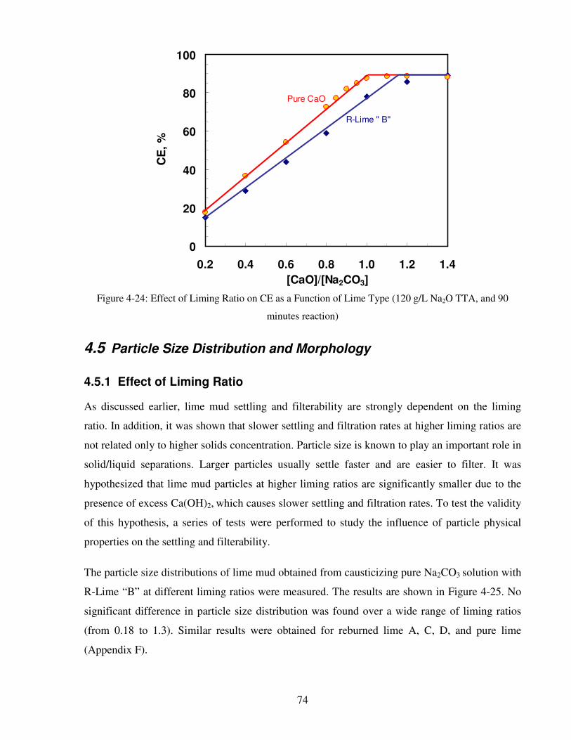
74

Figure 4-24: Effect of Liming Ratio on CE as a Function of Lime Type (120 g/L Na2O TTA, and 90

minutes reaction)

4.5 Particle Size Distribution and Morphology

4.5.1 Effect of Liming Ratio

As discussed earlier, lime mud settling and filterability are strongly dependent on the liming

ratio. In addition, it was shown that slower settling and filtration rates at higher liming ratios are

not related only to higher solids concentration. Particle size is known to play an important role in

solid/liquid separations. Larger particles usually settle faster and are easier to filter. It was

hypothesized that lime mud particles at higher liming ratios are significantly smaller due to the

presence of excess Ca(OH)2, which causes slower settling and filtration rates. To test the validity

of this hypothesis, a series of tests were performed to study the influence of particle physical

properties on the settling and filterability.

The particle size distributions of lime mud obtained from causticizing pure Na2CO3 solution with

R-Lime “B” at different liming ratios were measured. The results are shown in Figure 4-25. No

significant difference in particle size distribution was found over a wide range of liming ratios

(from 0.18 to 1.3). Similar results were obtained for reburned lime A, C, D, and pure lime

(Appendix F).

0

20

40

60

80

100

0.2 0.4 0.6 0.8 1.0 1.2 1.4

[CaO]/[Na2CO3]

CE

, %

Pure CaO

R-Lime " B"

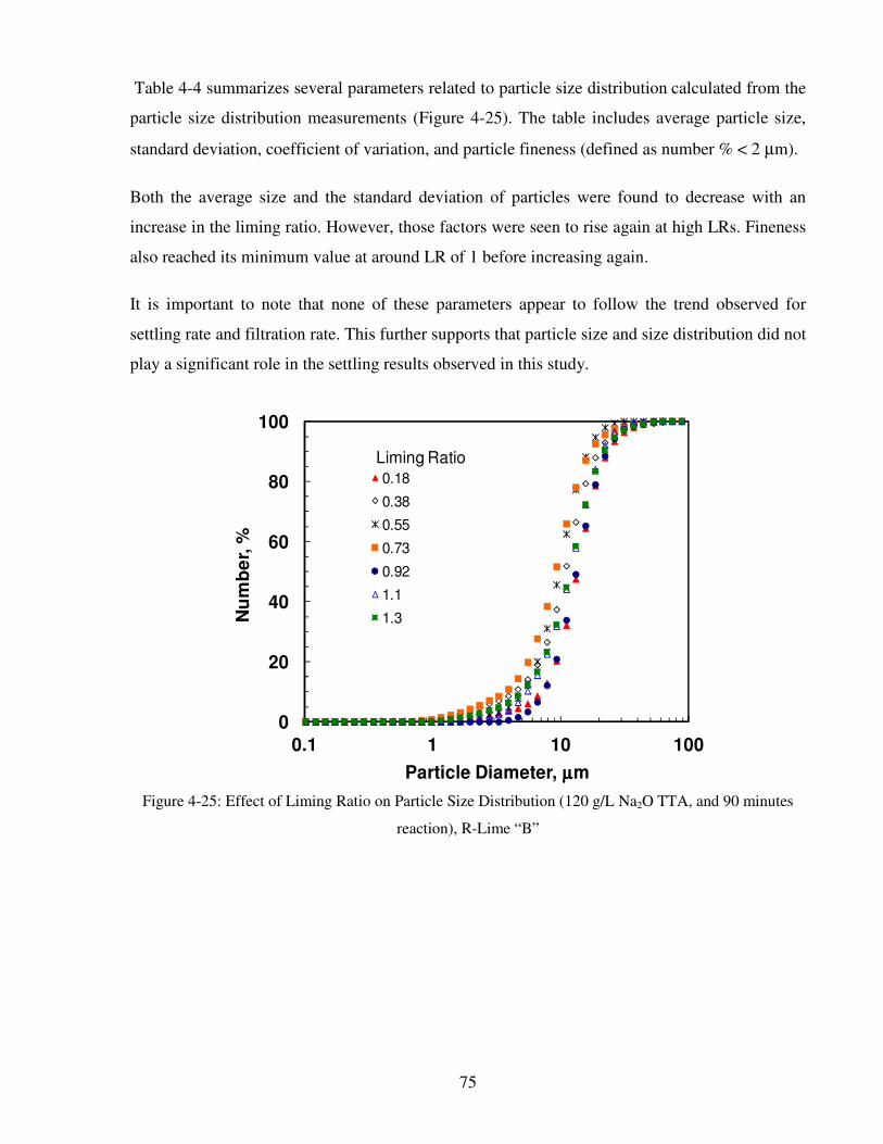
75

Table 4-4 summarizes several parameters related to particle size distribution calculated from the

particle size distribution measurements (Figure 4-25). The table includes average particle size,

standard deviation, coefficient of variation, and particle fineness (defined as number % < 2 µm).

Both the average size and the standard deviation of particles were found to decrease with an

increase in the liming ratio. However, those factors were seen to rise again at high LRs. Fineness

also reached its minimum value at around LR of 1 before increasing again.

It is important to note that none of these parameters appear to follow the trend observed for

settling rate and filtration rate. This further supports that particle size and size distribution did not

play a significant role in the settling results observed in this study.

Figure 4-25: Effect of Liming Ratio on Particle Size Distribution (120 g/L Na2O TTA, and 90 minutes

reaction), R-Lime “B”

0

20

40

60

80

100

0.1 1 10 100

Nu

mb

er,

%

Particle Diameter, µµµµm

0.18

0.38

0.55

0.73

0.92

1.1

1.3

Liming Ratio

76

Table 4-4: Summary of Parameters Related to Size Distribution

LR Average Particle

Diameter (µm)

Standard

deviation (µm)

Coefficient of

Variation (%)

Fineness

(%)

0.18 16 8.4 52 1.5

0.38 13.2 8.7 66 4.0

0.55 11.2 5.0 45 0.9

0.73 11.1 7.0 64 4.3

0.92 15.8 7.3 47 0

1.1 13.9 6.9 50 0.4

1.3 14.2 8.4 59 2.1

Figure 4-26 presents the particle diameter by number at the 85th

percentile as a function of liming

ratio. The 85th

percentile diameters were obtained from particle size distribution measurements

(Figure 4-25). No apparent correlation between liming ratio and particle diameter was found.

Figure 4-26: Relationship between Liming Ratio and 85th Percentile Diameter shown in Figure 4-25

0

5

10

15

20

25

0 0.5 1 1.5

85

thP

erc

en

tile

Dia

me

ter,

µµ µµm

[CaO]/[Na2CO3]

77

The measured 85th

percentile diameter of particles was subsequently used to examine their effect

on the particle settling velocity calculated in Section 4.2. As illustrated in Figure 4-27, there was

no significant correlation between these two parameters. This graph further confirms that there is

no apparent relation between lime mud particle size and settling velocity of particles as a

function of liming ratio.

Note: the two points at 20.6 µm display very different settling velocities, the reasons for this will be addressed

in Section 4.7

Figure 4-27: Comparing the 85th Percentile Diameter with Settling Velocity of Mud Particles as a

Function of Liming Ratio (120 g/L Na2O TTA, and 90 minutes reaction), R-Lime “B”

The surface area of mud particles were determined by the nitrogen adsorption technique BET as

described earlier. Figure 4-28 shows the specific surface area for the lime mud obtained from

causticizing pure Na2CO3 solution with pure CaO as a function of liming ratio. In general, the

smaller the particle size, the larger the particle surface area. As the results demonstrate, there is

no evidence that increasing the liming ratio resulted in an increase in specific surface area of

particles.

0

2

4

6

8

10 15 20

Se

ttli

ng

Ve

loc

ity,

cm

/min

85th Percentile Diameter, µµµµm

78

Figure 4-28: Effect of Liming Ratio on Specific Surface Area (120 g/L Na2O TTA, and 90 minutes

reaction), Pure CaO

Figure 4-29 shows scanning electron microscopy (SEM) images of lime mud samples obtained

from causticizing pure Na2CO3 solution with R-Lime “B” at different liming ratios. As shown,

no significant differences are evident in particle morphologies at different liming ratios. Analysis

of lime muds with SEM concluded that lime ratios does not have an impact on particle

morphologies.

From Figure 4-25 and Figure 4-26 and other results presented in this section, it is evident that the

variation in settling velocity and filtration rate cannot be explained simply based on the particle

size, size distribution, surface area, or particle morphology. The results suggest that particle size

does not change significantly with liming ratio, thus it is likely not the key factor affecting the

mud settling rate and filterability difficulties that are the focus of this study.

0

2

4

6

8

0.6 0.8 1 1.2 1.4

Su

rfa

ce

are

a m

2/g

[CaO]/[Na2CO3]

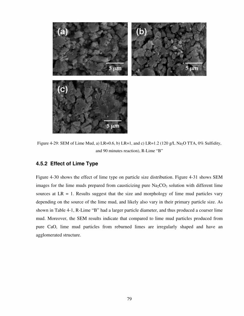
79

Figure 4-29: SEM of Lime Mud, a) LR=0.6, b) LR=1, and c) LR=1.2 (120 g/L Na2O TTA, 0% Sulfidity,

and 90 minutes reaction), R-Lime “B”

4.5.2 Effect of Lime Type

Figure 4-30 shows the effect of lime type on particle size distribution. Figure 4-31 shows SEM

images for the lime muds prepared from causticizing pure Na2CO3 solution with different lime

sources at LR = 1. Results suggest that the size and morphology of lime mud particles vary

depending on the source of the lime mud, and likely also vary in their primary particle size. As

shown in Table 4-1, R-Lime “B” had a larger particle diameter, and thus produced a coarser lime

mud. Moreover, the SEM results indicate that compared to lime mud particles produced from

pure CaO, lime mud particles from reburned limes are irregularly shaped and have an

agglomerated structure.

80

Figure 4-30: Particle Size Distribution of Different Lime Mud ([CaO] / [Na2CO3] =1, 120 g/L Na2O TTA,

and 90 minutes reaction)

Figure 4-31: SEM Images of Lime Mud Prepared from a) R-Lime “A”, b) R-Lime “B”, and c) Pure CaO

([CaO]/ [Na2CO3] =1, 120 g/L Na2O TTA, and 90 minutes reaction)

0

20

40

60

80

100

0.01 0.1 1 10 100


Nu

mb

er

%

R-Lime " A"

Pure CaO Liming Ratio = 1

R-Lime " B"

R-Lime " C"

R-Lime " D"

81

To compare the results of particle size measurements and filterability tests for the lime muds

prepared from causticizing pure Na2CO3 solution with different lime types at LR = 1, Sauter

mean particle diameters6 (d32) were determined from particle size measurements and plotted

against the calculated cake specific resistance presented in Table 4-3. Figure 4-32 shows the

results of this analysis. In general, there is a moderate correlation (R2 = 0.69) between the two

parameters. As expected, specific cake resistance decreased with an increase in particle size.

Figure 4-32: Correlation between Sauter Mean Particle Diameter and Specific Cake Resistance for

Different Lime Type ([CaO]/ [Na2CO3] =1, 120 g/L Na2O TTA, and 90 minutes reaction)

4.6 Evolution of Particle Size Distribution during Slaking and

Causticizing Reactions

The most commonly cited cause of mud settling and filterability difficulties is the presence of

free lime (unreacted Ca(OH)2) in the mud at higher liming ratios. Since Ca(OH)2 particles are

smaller than lime mud (CaCO3) particles, it is believed that free lime particles plug the precoat

filters, resulting in a low dewatering efficiency and consequently lime mud a with low solids

content [22].

6 Sauter mean diameter (d32) is commonly considered the mean size relevant to settling and filtration rate.

R-Lime"A"

R-Lime"B"

R-Lime"C"

R-Lime"D"

Pure CaO

y = -0.10x + 1.34R² = 0.69

0

0.5

1

1.5

0 5 10 15

Sp

ec

ific

Ca

ke

Re

sis

tan

ce×

10

-10,

m/k

g

Sauter Mean Particle Diameter (d32), µµµµm

82

To investigate the validity of the above hypothesis, two sets of experiments were designed to

study physical properties, settling, and filtration behaviour of Ca(OH)2 and CaCO3 particles

separately.

• In the first set of experiments, R-Lime “B” was added to water to produce Ca(OH)2.

Also, R-Lime “B” was added to a Na2CO3 solution to produce CaCO3 according to the

slaking and causticizing reactions. The physical properties of the resulting Ca(OH)2 and

CaCO3 particles were then compared.

• In the second set of experiments, slaking and causticizing reactions were performed by

adding R-Lime “B” to Na2CO3 solution. Samples were taken during the reactions to study

changes in physical properties of mud particles with the progression of the reactions.

4.6.1 Comparing Physical Properties of CaCO3 and Ca(OH)2 Particles

Figure 4-33 and Figure 4-34 compare the settling and filtration rates of CaCO3 and Ca(OH)2,

respectively.

Figure 4-33: Comparing Settling Curve for Ca(OH)2 and CaCO3 (R-Lime “B”, [CaO]/ [Na2CO3] =1, 120

g/L Na2O TTA, and 90 minutes reaction)

0

5

10

15

20

0 30 60 90

Inte

rfa

ce

He

igh

t, c

m

Time, min

CaCO3

Ca(OH)2

CaCO3

Ca(OH)2

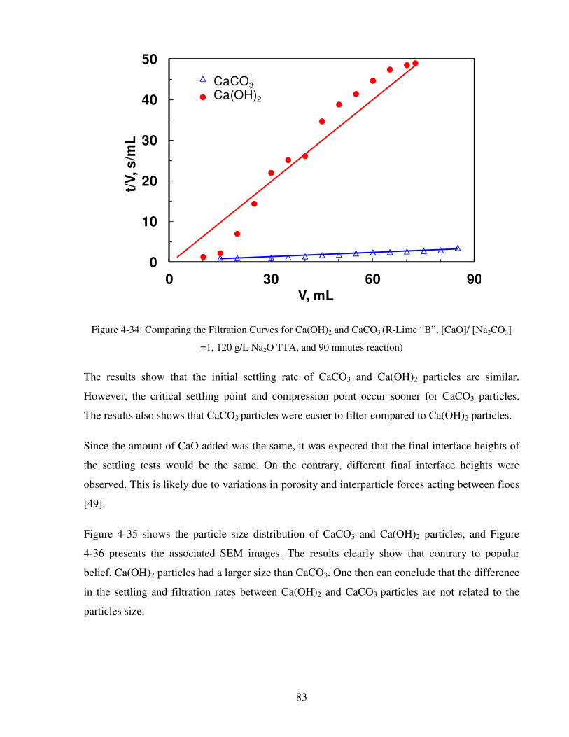
83

Figure 4-34: Comparing the Filtration Curves for Ca(OH)2 and CaCO3 (R-Lime “B”, [CaO]/ [Na2CO3]

=1, 120 g/L Na2O TTA, and 90 minutes reaction)

The results show that the initial settling rate of CaCO3 and Ca(OH)2 particles are similar.

However, the critical settling point and compression point occur sooner for CaCO3 particles.

The results also shows that CaCO3 particles were easier to filter compared to Ca(OH)2 particles.

Since the amount of CaO added was the same, it was expected that the final interface heights of

the settling tests would be the same. On the contrary, different final interface heights were

observed. This is likely due to variations in porosity and interparticle forces acting between flocs

[49].

Figure 4-35 shows the particle size distribution of CaCO3 and Ca(OH)2 particles, and Figure

4-36 presents the associated SEM images. The results clearly show that contrary to popular

belief, Ca(OH)2 particles had a larger size than CaCO3. One then can conclude that the difference

in the settling and filtration rates between Ca(OH)2 and CaCO3 particles are not related to the

particles size.

0

10

20

30

40

50

0 30 60 90

t/V

, s

/mL

V, mL

CaCO3

Ca(OH)2

CaCO3

Ca(OH)2

84

Figure 4-35: Comparing Particle Size Distribution for Ca(OH)2 and CaCO3 (R-Lime “B”, [CaO]/

[Na2CO3] =1, 120 g/L Na2O TTA, and 90 minutes reaction)

Figure 4-36: SEM of a) Ca(OH)2 Particles, and b) CaCO3 Particles (R-Lime “B”, [CaO]/ [Na2CO3] =1,

120 g/L Na2O TTA, and 90 minutes reaction)

Further, based on Figure 4-35, the particle size distribution of Ca(OH)2 is broader than that of

CaCO3, resulting in better packing of cake and a denser cake (Figure 4-34). A wider particle size

distribution gives a more densely packed cake, with smaller particles filling the spaces between

0

20

40

60

80

100

0.1 1 10 100 1000

Nu

mb

er

%

Particle Diameter (µµµµm)

Ca(OH)2

CaCO3

Ca(OH)2

CaCO3

5 µ5 µ5 µ5 µm

(a)

5 µ5 µ5 µ5 µm

(b)

5 µ5 µ5 µ5 µm

(a)

5 µ5 µ5 µ5 µm

(b)

85

larger particles. Also, this broad distribution can explain the differences in Figure 4-33; larger

particles settle first, resulting in a higher initial settling rate, but then smaller particles that are

left behind settle more slowly resulting in a steady but very shallow slope of the settling curve at

longer settling times in Figure 4-33.

4.6.2 Taking Samples During Slaking and Causticizing Reactions

To further study changes in physical properties of mud particles as a function of the progression

of the slaking and causticizing reactions, samples were taken at specified time intervals. The

slaking and causticizing reactions followed the procedure outlined in Section 3.1. Reburned lime

from Mill B and pure Na2CO3 were used in this test. Using a 10 mL syringe, samples were taken

at specified times and analyzed for composition and particle size. The intent was to differentiate

between CaCO3 and Ca(OH)2 behaviours. The reactor temperature was monitored using a

thermocouple.

Figure 4-37 shows the temperature profile of the reactor as a function of reaction time. The

temperature rose from 83 ºC to 97 ºC in the first 8 minutes during the slaking reaction where

hydration of calcium oxide took place and then consistently decreased to 73 ºC during the

causticizing reaction.

Figure 4-37: Temperature Profile During the Slaking and Causticizing Reactions

50

60

70

80

90

100

0 30 60 90

Te

mp

era

ture

, ºC

Reaction Time, min

86

Samples were analyzed by XRD to characterize their chemical make-ups. Figure 4-38 (a) to (c)

shows the XRD spectra of samples. The first spectrum shows the diffraction pattern of R-Lime

“B” which consists of CaO and small amounts of Ca(OH)2. The second spectrum shows the

reaction 5 minutes after adding reburned lime to the reactor. The second spectrum includes

strong characteristic peaks of the less crystalline Ca(OH)2 and to a lesser degree CaCO3 that has

a higher degree of crystallinity. It is important to note that the area under the characteristic peaks

represents the relative mass percentage of each component. This shows that the slaking reaction

proceeded to completion and that the causticizing reaction progressed considerably after 5 min.

The spectrum also included minor characteristic peaks of CaO, which shows that a small portion

of CaO remained unreacted. The third spectrum shows that the sample that was taken after 60

minutes consists of CaCO3 with a minor quantity of Ca(OH)2. The results demonstrate the

progression of the slaking and causticizing reactions as expected and were used to interpret the

outcome of particle size distribution tests.

Figure 4-39 shows the effect of reaction time on the particle size distribution. The particle sizes

decreased as the reactions progressed. For example, the sample taken after a 5-minute reaction

was a mixture of Ca(OH)2 and CaCO3 with large particles, while the sample taken after 30

minutes was almost entirely made of CaCO3 and had smaller particles.

This finding challenges the common belief that the generation of smaller size Ca(OH)2 particles

during the slaking and causticizing reactions is the root cause of settling and filterability

difficulties [24]. The results show that the products of the slaking and causticizing reactions are

progressively smaller in size with increasing reaction progress. As shown in Section 4.5, it is also

important to note that the particle size of lime muds did not change considerably with increases

in the liming ratio, and, as a result, the current observation should be valid for a range of liming

ratios. This further suggests that even at high liming ratios relatively large-size Ca(OH)2 particles

are potentially produced, but these are unlikely to plug the precoat filters. Instead the presence of

unreacted free lime could possibly form CaCO3 within the filter medium (cloth) and eventually

clog-up the cloth, resulting in a low dewatering efficiency and lime muds with low solids

content.

87

Figure 4-38: The XRD Results of the Sample (a) Reburned Lime, (b) 5-Minute Slaking and Causticizing

Reactions, and (c) 60-Minute Slaking and Causticizing Reactions, R-Lime “B” ([CaO]/ [Na2CO3] =1)

(a) CaO

Ca(OH)2

20 30 40 50 60

600

400

200

0

Position [ºTheta]

Counts/s

CaO

20 30 40 50 60

200

100

0

Position [ºTheta]

(b)

Counts/s

Ca(OH)2CaCO3

20 30 40 50 60

400

200

0

Position [ºTheta]

(c)

Counts/s

Ca(OH)2CaCO3

88

Figure 4-39: Particle Size Distribution of Lime Mud Throughout the Slaking and Causticizing Reactions

([CaO]/ [Na2CO3] =1, 120 g/L Na2O TTA, and R-Lime “B”)

4.7 Zeta Potential

In the previous sections, the effect of different parameters on the settling and filterability of lime

muds was studied. The results confirmed the strong dependence of settling and filterability on

the liming ratio. The validity of several hypotheses and common beliefs were shown to be

incorrect; while settling and filterability are indeed influenced by solids content and particle size,

they are not the main causes of poor filtration of lime mud.

If the lime mud particle size is smaller than 10 µm, the surface charge on the particles, which is

often represented by the zeta potential (ζ), becomes more prominent, and the net attractive or

repulsive forces between particles can become as significant as gravitationally or

hydrodynamically induced forces. Since the lime mud particle size does not change considerably

with increases in the liming ratio, it was decided to study the effect of surface charge on the

settling and filterability. For these tests, the experimental procedure described in Section 3.7 was

followed.

0

20

40

60

80

100

0.01 0.1 1 10 100 1000

Vo

lum

e (

%)

Particle Diameter (µµµµm)

1-Minute

5-Minute

30-Minute

90-Minute

Reaction Time

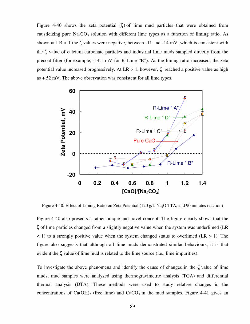
89

Figure 4-40 shows the zeta potential (ζ) of lime mud particles that were obtained from

causticizing pure Na2CO3 solution with different lime types as a function of liming ratio. As

shown at LR < 1 the ζ values were negative, between -11 and -14 mV, which is consistent with

the ζ value of calcium carbonate particles and industrial lime muds sampled directly from the

precoat filter (for example, -14.1 mV for R-Lime “B”). As the liming ratio increased, the zeta

potential value increased progressively. At LR > 1, however, ζ reached a positive value as high

as + 52 mV. The above observation was consistent for all lime types.

Figure 4-40: Effect of Liming Ratio on Zeta Potential (120 g/L Na2O TTA, and 90 minutes reaction)

Figure 4-40 also presents a rather unique and novel concept. The figure clearly shows that the

ζ of lime particles changed from a slightly negative value when the system was underlimed (LR

< 1) to a strongly positive value when the system changed status to overlimed (LR > 1). The

figure also suggests that although all lime muds demonstrated similar behaviours, it is that

evident the ζ value of lime mud is related to the lime source (i.e., lime impurities).

To investigate the above phenomena and identify the cause of changes in the ζ value of lime

muds, mud samples were analyzed using thermogravimetric analysis (TGA) and differential

thermal analysis (DTA). These methods were used to study relative changes in the

concentrations of Ca(OH)2 (free lime) and CaCO3 in the mud samples. Figure 4-41 gives an

-20

0

20

40

60

0 0.2 0.4 0.6 0.8 1 1.2 1.4

[CaO]/[Na2CO3]

Ze

ta P

ote

nti

al,

mV

R-Lime " C"

R-Lime " B"

R-Lime " D"

R-Lime " A"

Pure CaO

90

example of TGA/DSC results for lime muds obtained from the causticizing reaction of pure

Na2CO3 and pure CaO at LR = 1.4. The initial heat flow occurs at approximately 100 °C due to

the evaporation of moisture from the chemicals (dehydration). The second endothermic peak

shows a loss of mass at around 380 °C caused by the decomposition of Ca(OH)2. The third and

the most intense endothermic peak started at 650 °C and finished around 830 °C. This peak was

caused by the decomposition of CaCO3 to CaO.

Figure 4-42 plots the TGA weight loss profiles of lime mud obtained from the causticizing

reactions of CaO and Na2CO3 at different liming ratios. The weight loss due to decomposition of

Ca(OH)2 in mud samples increases with an increase in liming ratio, suggesting that causticizing

at higher liming ratios results in lime muds with a higher free lime (Ca(OH)2) content.

Figure 4-41: Weight Loss Profile for Lime Mud in Nitrogen (Pure CaO, [CaO]/ [Na2CO3] =1.4, 120 g/L


-12

-10

-8

-6

-4

-2

0

2

0

20

40

60

80

100

120

0 200 400 600 800 1000

He

at,

W/g

We

igh

t L

os

s, %

Temperature, ºC

91

Figure 4-42: TGA of Lime Mud Samples (Pure CaO, 120 g/L Na2O TTA, and 90 minutes reaction)

Figure 4-43 shows the Ca(OH)2 content of mud samples as a function of liming ratio for different

lime sources. Similar to above, the results indicate that with an increase in the liming ratio, the

free lime (Ca(OH)2) content increased.

Figure 4-43: Free Lime Contents as a Function of Liming Ratio

50

60

70

80

90

100

0 200 400 600 800 1000

We

igh

t L

os

s, %

Temperature, OC

0.40.811.21.4

[CaO]/[Na2CO3]

0

5

10

15

20

25

0 0.2 0.4 0.6 0.8 1 1.2 1.4 1.6

Ca

(OH

) 2,

wt%

[CaO]/[Na2CO3]

Pure CaO

R-Lime "A"

R-Lime "B"

R-Lime "C"

R-Lime "D"

92

These results are consistent with literature findings that the Ca2+

concentration has a profound

effect on the ζ of particles [68, 72]. It has been shown that increasing Ca2+

concentration in the

slurry causes the ζ to shift toward a more positive value due to the Ca2+

adsorption on the

negative sites on the calcite surface. Huang et al. [118] demonstrated that increasing Ca2+

in the

suspension makes the calcite surface more positively charged (i.e., increasing ζ) until the calcite

surface was saturated with Ca2+

ions.

Vergouw et al. [119] reported that the settling rate of galena (lead ore mineral) decreased in the

presence of Ca2+

ions. Huang et al. [118] also showed that the adsorption of Ca2+

onto calcite

particles is due to the strong affinity of Ca2+

for the calcite surface. That is, the Ca2+

ions

penetrate into the hydrolyzed layer, replace the water at the surface, and directly bind to the

calcite surface. As shown in Sections 4.2 and 4.3, lime mud settling and filtration rates decreased

noticeably with an increase in the liming ratio. In addition, as shown in Figure 4-27, the two

points with particle diameters of 20.6 µm (LR=0.18 and LR=0.92) display very different settling

velocities (7.2 cm/min and 0.34 cm/min), this behaviour is due to their differing zeta potential

values (Figure 4-40). The current findings, along with other evidence [119], suggest that lime

mud settling and filtration rates are strongly related to the concentration of Ca2+

ions in the

system. This further confirms that causticizing at higher liming ratios results in a higher free lime

(Ca(OH)2, or Ca2+

ions) content. This in turn changes the ζ value of lime mud and it makes

difficult to settle and filter.

Although different lime types demonstrated similar behaviour, the influence of lime sources on

the value of ζ was evident. Generally, polyvalent ions (e.g., PO43-

, HPO42-

, SO42-

, CO32-

, Mg2+

,

Ca2+

) tend to change the surface charge due to adsorption onto the opposite charged surface sites

and/or precipitation of another mineral onto the calcite surface. This means that the presence of

other ions as impurities depending on the type of ion and its concentration in the lime can alter

the ζ and have an effect on the mud settling and filterability.

Figure 4-44 shows the relationship between ζ and free lime contents of mud samples produced

from different sources of lime. In all five cases, increasing the free lime resulted in a higher ζ,

suggesting that a larger liming ratio may in fact increase the repulsive force between particles,

which hinders lime mud settling and filterability. Within the limits of experimental error, the

relationship between the free lime content and the ζ of the mud solution appears to be linear (R2

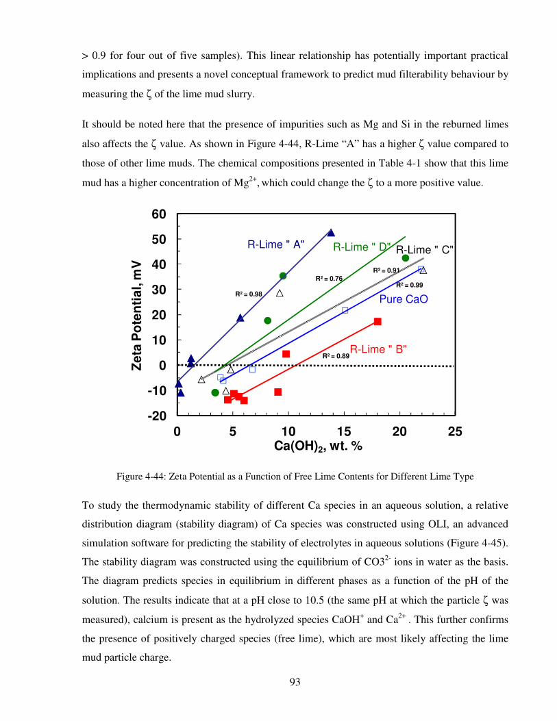
93

> 0.9 for four out of five samples). This linear relationship has potentially important practical

implications and presents a novel conceptual framework to predict mud filterability behaviour by

measuring the ζ of the lime mud slurry.

It should be noted here that the presence of impurities such as Mg and Si in the reburned limes

also affects the ζ value. As shown in Figure 4-44, R-Lime “A” has a higher ζ value compared to

those of other lime muds. The chemical compositions presented in Table 4-1 show that this lime

mud has a higher concentration of Mg2+

, which could change the ζ to a more positive value.

Figure 4-44: Zeta Potential as a Function of Free Lime Contents for Different Lime Type

To study the thermodynamic stability of different Ca species in an aqueous solution, a relative

distribution diagram (stability diagram) of Ca species was constructed using OLI, an advanced

simulation software for predicting the stability of electrolytes in aqueous solutions (Figure 4-45).

The stability diagram was constructed using the equilibrium of CO32-

ions in water as the basis.

The diagram predicts species in equilibrium in different phases as a function of the pH of the

solution. The results indicate that at a pH close to 10.5 (the same pH at which the particle ζ was

measured), calcium is present as the hydrolyzed species CaOH+ and Ca

2+ . This further confirms

the presence of positively charged species (free lime), which are most likely affecting the lime

mud particle charge.

R² = 0.98

R² = 0.89

R² = 0.99

R² = 0.91

R² = 0.76

-20

-10

0

10

20

30

40

50

60

0 5 10 15 20 25

Ze

ta P

ote

nti

al,

mV

Ca(OH)2, wt. %

R-Lime " A" R-Lime " D"

R-Lime " B"

Pure CaO

R-Lime " C"

94

Figure 4-45: Species Distribution Diagram as a Function of pH

Figure 4-46 plots the average settling rate of lime mud particles as a function of zeta potential.

The average settling rate was determined from the slope of the settling curves. The batch settling

tests were carried out at a constant solids concentration of 20 wt. % as a function of the liming

ratio. A point on this curve represents the settling velocity of lime mud at a specific liming ratio.

This figure indicates a sharp drop in the settling velocity of lime mud with an increase in the ζ

from -14 to -5 mV. As the ζ increases, the settling velocity decreases slowly to a small value. For

a given lime mud source, the average settling rate is much greater when the ζ is negative than

when it is positive. The decrease in the settling rate, however, becomes less pronounced as the ζ

becomes positive.

Figure 4-47 shows the filtration rate of produced lime mud as a function of ζ. Results indicate a

good inverse linear relationship between these two parameters. It is apparent that an increase in

the ζ, which is directly related to an increase in the liming ratio, leads to a decrease in the

filtration rate of the lime mud from 2.1 to 0.6 g/s.

-6

-5

-4

-3

-2

-1

0

3 5 7 9 11 13

Lo

g C

on

ce

ntr

ati

on

(m

ol/

L)

pH

CaCO3 (s)Ca 2+

H2CO3

HCO3-

CaHCO3+

CaOH+

CaCO3 (Aq)

CO32-

95

Figure 4-46: Average Settling Velocity vs. Zeta Potential of Particles (Constant Concentration: 20 wt. %,

120 g/L Na2O TTA, and 90 minute reaction)

Figure 4-47: Filtration Rate vs. Zeta Potential of Particles (Constant Concentration: 20 wt. %, 120 g/L

Na2O TTA, and 90 minutes reaction), R-Lime “A”, R-Lime “B”, and Pure CaO

0

0.1

0.2

0.3

0.4

0.5

-20 0 20 40 60

Se

ttli

ng

Ve

loc

ity,

cm

/min

ζζζζ, mV

R-Lime " A"R-Lime " D"

Pure CaO

R-Lime " B"

R-Lime " C"

y = -0.04x + 1.48R² = 0.94

0

0.5

1

1.5

2

2.5

-20 -10 0 10 20 30

Fil

tera

tio

n R

ate

, g

/s

ζζζζ, mv

96

Figure 4-48 shows the correlation between the ζ of lime mud particles and causticizing

efficiency (CE) at a specific liming ratio for different lime types. The CE values and ζ values

were determined from Figure 4-24 and Figure 4-40, respectively. The results suggest that ζ value

increases as CE increases. As shown, the graph can be divided into three sections. At the left side

of the graph, where CE values increased significantly, the ζ of particles were negative. However,

the lower the CE values, the more negative were the ζ values. This indicates that increasing the

CO32-

concentration would cause the ζ to shift to more negative values. There is a maximum

efficiency that could be attained for a given lime approximately at the zero value for ζ. This

implies that the zero ζfor lime mud occurs when the concentration of Ca2+

ions in the suspension

equals the concentration of CO32-

ions. Subsequently, while the ζvalues increased significantly,

the CE remained at the same value indicating that the increased Ca2+

concentration caused the ζ

to shift to more positive values. Hence, the magnitude of the ζ depended on the actual Ca2+

and

CO32-

concentrations.

Figure 4-48: CE vs. Zeta Potential of Particles (120 g/L Na2O TTA, and 90 minutes reaction), R-Lime

“A”, R-Lime “B”, and Pure CaO

Once the maximum possible CE was obtained, there would be no further reaction between

Ca(OH)2 and Na2CO3. Adding more lime (Ca(OH)2) than the maximum amount would overlime

0

20

40

60

80

100

-20 -10 0 10 20 30 40 50 60

CE

, %

ζζζζ ,mV

Pure Lime

R-Lime"A"

R-Lime"B"

97

the system, while adding less lime would underlime the system. As a result, there exists a

maximum liming ratio above which the system would be overlimed. Thus, the higher the ζ, the

easier it would be for the system to be overlimed.

98

5 Relationship between Zeta Potential and Kozeny

Coefficient

Results presented in Chapter 4 suggest that the zeta potential (ζ) of lime mud affects its settling

characteristics. In order to gain a better understanding of this phenomenon, a theoretical model

was used to predict the settling rate of mud particles. To plot a batch settling curve, i.e., the

change in the height of the interface between the supernatant (clear liquid) and the settling

suspension with respect to time, the Holdich and Butt model [30] was adapted. A description of

the theory of the batch settling curve and their mathematical model is provided in Section 2.1.1.

The model was modified by comparing the theoretical settling rates with the experimental data.

A linear relationship was then established between the ζ and the Kozeny coefficient to account

for the effect of particle surface charge on the settling rate.

5.1 Results and Discussion

5.1.1 General Approach

Experimental results which have been presented in Section 4.5 show that the liming ratio has

little effect on the particle size distribution. To compliment the experimental results with an

analytical study using the Holdich and Butt model, batch settling curves were plotted and

compared with the experimental settling curves. The experimental data used were settling test

results of the lime mud that was obtained from causticizing pure Na2CO3 solution with Mill B

lime as a function of liming ratio at a constant concentration of 6 wt. % (Figure 4-11).

99

Figure 5-1 shows a comparison between the experimental data for the highest and the lowest

liming ratios and the theoretical curves for the smallest and largest particle diameters detected in

the lime mud samples. As shown, there was a significant difference between the experimental

and theoretical settling rates, suggesting that the low settling rate as a result of an increase in the

liming ratio was not only due to the particle size.

Figure 5-1: Theoretical and Experimental Settling Rates

5.1.2 Kozeny Coefficient

To better understand the cause of the discrepancy between the experimental and predicted

settling curves, a parametric study was conducted to examine the effect of the Kozeny coefficient

variation on the settling rate.

The particles were assumed to be spherical with a diameter of 15 µm and density of 2600 kg/m3

that were settling in a water column with a height of 13.0 cm at an initial concentration of 5 % by

volume. The predicted settling curves for different values of the Kozeny coefficient (K) are

shown in Figure 5-2.

0

5

10

15

0 10 20 30Time, min

Inte

rfa

ce

He

igh

t, c

mExperimental Data - Smallest

and Largest Liming Ratio

Calculated - Largest and

Smallest Particle Diameter

100

Figure 5-2: Effect of Kozeny Coefficient on Settling Curve (Particle Diameter = 15 µm, and Initial

Concentration = 5 % v/v)

The results indicate that with an increase in K, the settling rates of particles increased

significantly. This finding suggests that changes in the value of K may be responsible for the

observed deviation between theoretical predictions and the experimental data in Figure 5-1. To

evaluate this hypothesis, the theoretical settling curves were fitted to the experimental data based

on the least square analysis while using K as the fitting parameter.

The values of K obtained for different liming ratios and the calculated settling curves are given

in Table 5-1 and Figure 5-4, respectively. According to Table 5-1, K appears to increase with

increasing ζ of lime mud samples. This relationship is better illustrated in Figure 5-3 where a

strong linear correlation (R2 = 0.90) between the K and ζ of samples is observed.

It should be noted that the Kozeny coefficient K is inversely proportional to the permeability

coefficient k according to Equation (8). k, in turn, depends on fluid density and material porosity

according to Darcy’s law (Equation (11)). A greater Kozeny coefficient means a lower

permeability and a lower rate of fluid flowing through a material, or slower settling and

dewatering rates.

0

2

4

6

8

10

12

14

0 20 40 60

Inte

rfa

ce

He

igh

t, c

m

Time, min

K=1.75

K=3.36

K=5

K=15

K=23

101

It is expected that if ζ values show a higher negative value (due to the presence of ions that cause

the surface charge of lime mud particles to become negatively charged), the Kozeny coefficient

will be increased. This means that the relationship between ζ and Kozeny coefficients could be

hyperbolic. However, this cannot be confirmed with the limited data shown in Figure 5-3,

because no experiments were conducted in this study that could produce high negative ζ values.

Table 5-1: Summary of Zeta Potential of Particles and Estimated Kozeny Coefficients

Liming Ratio, LR ζ, mV Kozeny Coefficient, K 0.38 -11.3 1

0.73 -12.4 1.5

0.92 -10.6 2.5

1.1 +4.5 3.4

1.3 +17.3 5

For smaller particles, the interparticle forces are expected to play a dominant role in the settling

and packing of particles. By increasing the ζ, the particles separate from each other due to their

stronger repulsive forces [120]. Hence, the net effect of such particle-particle interactions would

resemble that of increased particle size and consequently an increase in K.

102

Figure 5-3: Linear Relationship between Zeta Potential and Kozeny Coefficient

Figure 5-4: Experimental and Calculated of Lime Mud Settling Curves (Mill B Lime at a Constant

Concentration of 5 % v/v)

y = 0.12x + 2.96R² = 0.90

0

1

2

3

4

5

6

-20 -10 0 10 20

Ko

ze

ny C

oe

ffic

ien

t

ZP, mV

0

2

4

6

8

10

12

14

0 5 10 15 20 25 30

Time, min

Inte

rfa

ce

He

igh

t, c

m

Experimental 0.38

Calculated 0.38

Experimental 0.73

Calculated 0.73

Experimental 0.92

Calculated 0.92

Experimental 1.1

Calculated 1.1

Experimental 1.3

Calculated 1.3

Liming Ratio

103

5.2 Parametric Study: Effect of Particle Size and Concentration

5.2.1 Effect of Particle Size on Settling Rate of CaCO3 Particles

A parametric study was performed to determine the effect of particle size on the settling of

CaCO3 particles using the analytical methods described above. Figure 5-5 shows the effect of the

particle size on the settling rate of mud particles. In this figure, the particle diameter was varied

from 2 to 75 µm while the Kozeny coefficient was kept constant at 2.5 (K value at LR = 1). As

expected, the settling rate increased steadily as the particle size decreased. For larger particle

sizes, the particle settling occurred more quickly. For particles of 75 µm, for example, the

interface height decreased from 14 cm to 1 cm within the first minute and was constant

thereafter. For particles of 2 µm, on the other hand, the interface height did not decrease much

even after 30 minutes.

In practice, particles smaller than 2 µm settle more slowly than what is predicted by Stokes’ law,

and particles less than 1 µm in size do not settle at all [32]. On the other hand, at a particle

diameter greater than 100 µm (i.e., a Reynolds number > 0.2) the degree of turbulence becomes

more important [34]. Thus, the particle velocity is lower than that predicted by Stokes’ law.

Figure 5-6 shows the settling velocities calculated as the slope of the settling curves within the

zone settling regime. The results are consistent with Equation (9), which predicts that the settling

velocity increases proportional to dp2.

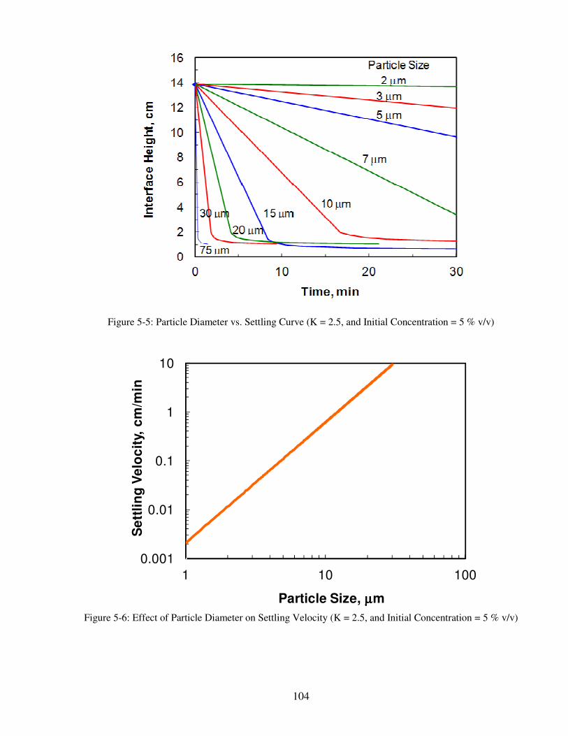
104

Figure 5-5: Particle Diameter vs. Settling Curve (K = 2.5, and Initial Concentration = 5 % v/v)

Figure 5-6: Effect of Particle Diameter on Settling Velocity (K = 2.5, and Initial Concentration = 5 % v/v)

0.001

0.01

0.1

1

10

1 10 100

Se

ttli

ng

Ve

loc

ity,

cm

/min

Particle Size, µµµµm

105

5.2.2 Effect of Initial Solids Content on Settling Rate of CaCO3 Particles

Figure 5-7 shows the effect of the initial solids content on the settling rate for spherical CaCO3

particles with a diameter of 15 µm and a density of 2600 kg/m3 at different initial solids contents

ranging from 1 to 50 % v/v. A constant Kozeny coefficient of 2.5 (K value at LR = 1) was used

in this case. Settling curves were plotted using the analytical method described in Section 5.1.2.

In general, hindered settling occurred when the particle concentration was greater than 1 % v/v.

Particles did not settle if the sediment concentration was in excess of 60 % solids, and the more

diluted the slurry had higher settling rates. Therefore, the most commonly used values are

typically between 20 and 30 % v/v, as diluting to lower values would result in increased volume

capacities of the settling vessels.

As expected, the settling rate of particles decreased progressively as the concentration of the

suspension was increased. The higher concentration samples gave slower particle settling rates.

At 1 % v/v, the interface height dropped from 14 cm to 0.5 cm within the first minute and

became constant thereafter. At 50 % v/v, on other hand, the interface height changed only

slightly after the first 30 minutes.

The settling velocities were calculated as the slope of the settling curves within the zone settling

regime (Figure 5-8). The results indicate that, as predicted from Equation (9), increasing the

solids content from 1 to 50 % v/v decreased the settling rate proportional to (1– C)3/C.

106

Figure 5-7: Initial Solids Content vs. Settling Curve (Particle Diameter = 15 µm, K = 2.5)

Figure 5-8: Effect of Initial Solids Content on Settling Velocity (Particle Diameter = 15 µm, K = 2.5)

0

5

10

15

0 20 40 60 80 100

Se

ttli

ng

Ve

loc

ity,

cm

/min

(1-C)3/C

107

6 Practical Implications

This study confirms that the mud settling rate and filterability decrease with an increase in liming

ratio. The decrease is much more notable as the liming ratio exceeds a critical level determined

by the causticizing equilibrium. Poor mud settling and filterability are not caused by the small

particle size of Ca(OH)2 (free lime) as commonly believed, but by an increase in the zeta

potential of Ca(OH)2-containing mud particles. The zeta potential of the particles changes from

slightly negative when the system is underlimed to strongly positive when the system is

overlimed.

The study also identifies a linear relationship between the zeta potential and the free lime content

for different sources of lime. This implies that operating the causticizing system near the

isoelectric point (zero zeta potential) would result in an optimum coagulation of charged

particles, which should improve the settling and filterability. Therefore, measuring the zeta

potential of the lime mud could estimate the free lime content and also avoid lime mud

filterability issues caused by overliming. This concept can be used in the development of a

practical tool for monitoring and adjusting lime addition to the slaking and causticizing vessels.

The new method is expected to provide a reliable and accurate replacement for the current

method of identification of overliming in pulp mills, known as the “5-minute settling test” [21].

The test procedure was described in Section 3.2.1.

108

7 Conclusions and Recommendations

7.1 Conclusions

A systematic laboratory study was carried out to examine the effect of liming ratio on the settling

rate and filterability of the lime mud produced by causticizing aqueous solutions of Na2CO3 with

pure and reburned limes from four different Canadian kraft mills. The main conclusions are

summarized as follows:

• Lime mud settling and filtration rates decreased with an increase in liming ratio,

regardless of lime type. The decrease was much more noticeable as the liming ratio

exceeded the overliming threshold.

• Overliming is the leading cause of settling and filterability difficulties.

• The slower settling was caused by both the higher liming ratio and the higher solids

concentration.

• There was no significant change in lime mud particle size with an increase in liming

ratio.

• Low settling rate and poor filterability are not caused by the small size of free lime

particles as commonly believed. They are rather caused by an increase in the zeta

potential of free lime particles.

• The zeta potential of lime particles changed from slightly negative to strongly positive

when the system state changed from underlimed to overlimed.

• The increasing trend between zeta potential and free lime content of the samples suggests

that the zeta potential measurements could be used to identify overliming.

• The magnitude of the zeta potential depends on the actual Ca2+

and CO32-

concentrations,

and the presence of impurities may considerably change the zeta potential of lime mud

particles.

109

• A zeta potential meter can be a practical tool for monitoring and adjusting lime addition

to the slaking and causticizing vessels in order to obtain optimum operating conditions in

the dewatering process.

• A batch settling curve was plotted using the Holdich and Butt model. A linear

relationship between zeta potential and Kozeny coefficient was established to correct the

effect of particle surface charge on the settling rate.

7.2 Recommendations

The present work identified several items for further investigation. These are outlined below:

• This work investigated the effect of liming ratio on the settling rate, filterability, and

characteristic properties of lime mud produced by causticizing aqueous solutions of

Na2CO3 with pure and reburned limes. It is suggested to further extend this work by

performing additional tests and studying the effect of liming ratio on the lime mud

dewatering by causticizing a solution of Na2CO3 and Na2S (green liquor) with pure and

reburned limes.

• It is recommended to study the effect of NPE (as impurities such as Mg, Si, P, Al, Fe) on

the lime mud properties and dewatering characteristics.

• It is important to study the effect of the type and concentration of impurities on the zeta

potential of lime mud samples. In an aqueous medium, zeta potential is also strongly

influenced by sample pH. The effect of pH on zeta potential measurements should also be

investigated.

• An experimental filterability apparatus should be developed to control cake thickness.

This would be useful in investigating the cake moisture content as a function of liming

ratios. It is recommended to conduct experiments to study the relationship among the

liming ratios, the cake moisture content, and the zeta potential of particles. The results

could be useful to finding optimum operating conditions of lime mud dewatering

processes.

110

• In the present work, physical and chemical properties of lime mud were studied after

drying the samples in an oven. It is suggested to study mud characteristics in wet

samples.

• It is strongly recommended to use the findings of this work to develop an analytical

method for determining overliming by the measurement of zeta potential.

111

8 Reference

1. Biermann, C. J., “Essential of Pulping and Papermaking”, Academic Press, San Diego,

1993.

2. Tran, H. N., Vakkiainnen, E. K., “Advances in the Kraft Chemical Recovery Process”, The

3rd

International Colloquium on Eucalyptus Pulp, Belo, Horizonte, Brazil, March 2007.

3. Tran, H. N., “The kraft Recovery Process”, Tappi Kraft Recovery Short Course, Tappi

Press, St. Petersburg, Florida, January 8-11, 2007.

4. Tran, H. N., “Energy and Chemical Recovery”, Chemical Engineering (CHE 564), Pulp

and Paper Course Notes, University of Toronto, Spring 2009.

5. Sanchez, D., “Recausticizing: Principles and Practice”, Tappi Kraft Recovery Short

Course, Tappi Press, St. Petersburg, Florida, January 8-11, 2007.

6. Papermaking Science and Technology: Chemical Pulping, Chapter 14, White liquor

Preparation, Book 6B, 2000: B133-202.

7. Adams, T.N., “Lime Kiln Principles and Operations”, TAPPI Kraft Recovery Course,

TAPPIPress, 2009.

8. Llyod, P. J., and Ward, A. S., “Filtration Applications of Particle Characterization”, AIChE

Series, 171(73), 1975: 6-12.

9. Tadros, M. E., and Mayes, I., “Effect of Particle Properties on Filtration of Aqueous

Suspensions”, Proceeding of the International Symposium on Fine Particle Processing,

Las Vegas, NV, 1980: 1583-1593.

10. Puttock, S. J., Frane A. G., Fell, C. J. D., Robins, R. G., and Wainwright, M. S., “Vacuum

Filtration and Dewatering of Alumina Tihydrate – The Role of Cake Porosity and Material

Phenomena”, International Journal of Mineral Processing, 17, 1986: 205-224.

11. Rong, R. X., and Hitchins, J., “Preliminary Study of Correlation between Fine Coal

Characteristics and Properties and their Dewatering Behaviour”, Minerals Engineering,

8(3), 1995: 293-309.

12. Ives, K. J., and Gregory, J., “Surface Forces in Filtration”, Journal of the Society for Water

Treatment and Examination, 15, 1996: 93-116.

13. Dolina, L. F., and Kaminski, V. S., “Influence of the Electrokinetic Charge Potential of

Particles on Dewatering Processes”, Coke Chem., 1, 1974: 8-11.

14. Ayub, A. L., and Sheppard, J. D., “Dewatering of Fuel Grade Peat with Surfactants –

Adsorption and Electrokinetics”, Colloid and Surfaces, 18, 1986: 43-52.

112

15. Chen, W.-J., “Effect of Surface Charge and Shear during Orthokinetics Flocculation on the

adsorption and Sedimentation of Kaolin Suspension in Polyelectrolyte Solutions”,

Separation Science and Technology, 33, 1998: 569-590.

16. Henderson, A. F., Cornell, C. F., Dunyon, A. F., and Dahlstrom, D. A., “Filtration and

Control of Moisture Content on Taconite Concentrates”, Tran. AIME, 204, 1957: 349-355.

17. Wakeman, R.J., “Filtration Post Treatment”, Elsevier, Amsterdam, 1975.

18. Wheelock, T. D., and Drzymala, J., “Coal Hydrophobicity and its Role in Filtration and

Dewatering”, Filtration and Separation, 28 (3), 1991: 351-354.

19. Rushton A., Hosseini, M., and Hassan, I., “The Effect of Velocity and Concentration on

Filter Cake Resistance”, Journal of Separation Processes Technology, 1, 1980: 35-41.

20. Stroh, G., and Stahl, W., “Effect of Surfactants on Filtration Properties of Fine Particle”,

Filtration and Separation, 27 (3), 1990: 197-199.

21. Angevine P. A. “How to Troubleshoot Problems that Arise in Mill Causticizing Systems”,

Pulp and paper, 128 (Dec.), 1979: 128-129,134.

22. Riberio, J. C., Santos, S., and Tran, H. “Experience of Low Mud Solids Problems at a Kraft

Pulp Mill”, Proceeding of the International Chemical Recovery Conference, Quebec City,

Canada, May 29-June 1, 2007: 567-573.

23. Dorris, G. M., and Allen, L. H., “The Effect of Reburned Lime Structure on the Rates of

Slaking, Causticizing and Lime Mud Settling”, Journal of Pulp and Paper Science, 11(4),

1985: J89-J98.

24. Dorris, G. M., “The Physical Characterization of Hydrated Reburned Lime and Lime Mud

Particles”, Journal of Pulp and Paper Science, 19(6), 1993: 256-167.

25. Campbell, A. J., “The Effects of Lime quality and Dosage on Causticizing and Lime Mud

Settling Properties”, Pulp & Paper Canada, 86(11), 1985:67-71.

26. Ruashton, A., Ward, A.S., and Holdich, R.G., “Solid-Liquid Filtration and Separation

Technology”, VCH Weinheim, 1996.

27. Stokes, G.G., Mathematical and Physical Papers, 3, Cambridge University Press,

Cambridge, 1891.

28. Richardson, J. F., and Zaki, W. N. “Sedimentation and Fluidization”, Trans. Inst. Chem.

Engers., 32, 1954: 35 -53.

29. Coe, H.S, and Clevenger, G.H., “Methods for Determining the Capacities of Slime Settling

Tanks”, Trans. Am. Inst, Mining Engrs, 55, 1916: 356-384.

30. Holdich, R.G., and Butt, G., “Solid/Liquid Separation by Sedimentation”, Journal of

Process Mechanical Engineering, 211, 1997: 43-52.

113

31. Kynch. G. J., “A Theory of Sedimentation”, Trans. Faraday Society, 48, 1952: 166-176.

32. Holdich, R.G “Fundamentals of Particle Technology”, Midland Information Technology

and Publishing, Nottingham, UK, 2003.

33. Holdich, R.G., and Butt, G., “Experimental and Numerical Analysis of a sedimentation

Forming Compressible Compacts”, Separation Science and Technology, 23(13), 1997:

2149-2171.

34. Coulson, J. M., Richardson, J.F., and Harker, J.H. “Chemical Engineering”, V. 2, Ed.5th

,

Oxford, Boston, Btterworth-Henemann, 1996.

35. Wakeman, R., “The influence of Particle Properties on Filtration”, Separation purification

Technology, 58, 2007: 234-241.

36. Holdich, R.G., “Rotary Vacuum Filter Scale-up Calculations and the Use of Computer

Spreadsheets”, Filtration & Separation, November and December, 1990: 435-439.

37. Kozeny J., Sitzber. Akad. Wiss. Wien, Math-naturnw. kl (Abt. Ha), 136, 1927:271.

38. Theliander, H., “On the Filtration Properties of Lime Mud”, Nordic Pulp and Paper

Research Journal, 5(2), 1990: 74-82.

39. Wang, W., and Chase, G. G., “Using Zeta Potentials to Characterize Filter Performance”,

Microscale Physiochemical Engineering Center (MPEC), The University of Akron, 2004.

40. Israelachivili, J.N., “Adhesion Forces between Surface in Liquid and Condensable

Vapours”, Surface Science Report, A review Journal, 14(3), 1992.

41. Butt, H._J., Graf, K., and Kappl, M., Physics and Chemistry Interface, Weinheim : Wiley-

VCH ; Chichester : John Wiley, 2003.

42. Hough, D.B., and White, L.R., “The Calculation of Hamaker Constant from Lifshitz

Theory with Application to Wetting Phenomena”, Adv. Colloid Interf. Sci., 14(3), 1980.

43. Goodwin, J.W., “Colloidal Dispersions”, Special Publication, 43, 1981

44. Aplan, F.F., and Fuerstenau, M.D, “Froth Flotation”, Fuerstenau, D.W., ed. AIME, New

York, 1962:170, 173.

45. Chapman, D. L., Phil. Mag. 25(6), 1913:475.

46. Stern, O.Z, .Electrochem, 30, 1924:508.

47. Hunter, R.J., “Zeta Potential in Colloid Science, Principles and Application”, Academic

Press, London, 1981.

48. Kruyt, H.R., Editors, Colloid Science, 1, 1952: 159, 199, 206

114

49. Henry, D.C, “The Cataphoresis of Suspended Particles, Part I: The Equation of

Cataforesis”, Proc. Roy. Soc., 133, 1931:106-129.

50. Overbeek, J.Th.G., “Colloid Science”, Elsevier, Amsterdam, 1952.

51. Michaels, A.S., and Bolger, J.C., “Settling Rates and Sediment Volumes of Flocculated

Kaolin Suspension”, Industrial Engineering Chemistry & Fundamentals, 1(1), 1962: 24-33.

52. Gaudin, A.M., and Fuerstenau, D.W., “The Transviewer-X-rays to Measure Suspended

Solids Concentration”, Engineering and Mining Journal, 159(2), 1958: 110-112.

53. Firth, B.A., “Flow Properties of Coagulated Colloidal Suspensions, II. Experimental

Properties of the Flow Curve Parameters”, Journal of Colloid and Interface Science, 57 (2),

1976: 257-265

54. Firth, B.A., and Hunter, R.J., “Flow Properties of Coagulated Colloidal Suspensions, II.

The Elastic Floc Model”, Journal of Colloid and Interface Science, 57 (2), 1976: 266-275.

55. Wright, H.J.L., and Kitchener, J.A., “The Problem of Dewatering Clay Slurries: Factors

Controlling Filterability”, Journal of Colloid and Interface Science, 56, 1976:57.

56. Fuerstenau, M.D., Gaudin, A.M., and Miaw, H.L., “The Influence of Alumina Slimes on

Galena Flotation,” American Institute of Mining, Metallurgical and Petroleum

Engineering, 211, 1958: 792 -795

57. Yopps. J.A., and Fuerstenau, D.W., “The Zero Point Charge of Alpha-alumina” Journal of

Colloid Science, 19 (1), 1964: 61-71

58. Boynton, R.S., “Chemistry and Technology of Lime and Limestone”, John Wiley & Sons,

INC., New York, 1980, Chapter Nine.

59. Hanson, C, and Theliander, H., “Properties and Quality of Lime, Part I: Influence of

Conditions during Reburning”, Nordic Pulp and Paper Research Journal, 9(3), 1994: 161-

166, 195.

60. Hanna, H. S., and Somasundaran, P., “Flotation of Salt Type Minerals”, Floatation –

Memorial Volume, 8, 1976: 197-272.

61. Madsen, L., “Surface Charge of Calcite”, Encyclopedia of Surface and Colloid Science,

Dekker, New York, 2002.

62. Somasundaran, P., and Agar, G. E., “The Zero Charge of Calcite”, Journal of Colloid

Interface Science, 24, 1967: 433-440.

63. Thompson, D. w., and Pownall, P. G., “Surface Electrical charges of Calcite”, Journal of

Colloid Interface Science, 131(1), 1989: 74-82.

115

64. Somasundaran, P., Amankonah, K., P., and Ananthapadmabhan, K., P., “Mineral –

Solution Equilibria in Sparingly Soluble Mineral System”, Colloid and Surfaces, 15, 1985:

309-333.

65. Eriksoon, R., Merta, J., and Rosenholm, J., B., “The Calcite/Water Interface I. Surface

Charge in Indifferent Electrolyte Media and the Influence of Low-molecular-weight

Polyelectrolyte”, Journal of Colloids and Interface Science, 313, 2007: 184-193.

66. Berlin, T. S., and Khabakov, A. V., “Difference in Electro-kinetic Potentials of Carbonate

Sedimentary Rocks of Different Origin and Composition”, Geochemistry, 3, 1961: 217-

230.

67. Siffert, B., and Fimbel, P., “Parameters Affecting the Sign and the Magnitude of the

Electrokinetic Potential of Calcite”, Colloid and Surfaces, 11, 1984: 377-389.

68. Smallwood, P. V., “Some Aspects of the Surface Chemistry of Calcite and aragonite, Part

I: An Electrokinetic Study”, Colloid Polymer Science, 255, 1977: 881-886.

69. Foxall, T., Peterson, G. C., Rendall, H. M., and Smith A. L., “Charge Determination of

Calcium Salt/ Aqueous Solution Interface”, Journal of the Chemical Society, Faraday

Transactions, 75 (I), 1979: 1034-1039.

70. Thompson, W. D., and Pownall, G. P., “Surface Electrical Properties of Calcite”, Journal

of Colloids and Interface Science, 131, 1989: 74-82.

71. Pierre, A., Lamarche, J. M., Mercier, R., and Foissy, A., “Calcium as Potential

Determining Ion in Aqueous Calcite Suspensions”, Journal of Dispersion Science and

Technology, 11, 1990: 611-635.

72. Stipp, S. L., and M. F. Hochella, Jr., “Structure and Bonding Environments at the Calcite

Surface as Observed with X-Ray Photoelectron Spectroscopy (XPS) and Low Energy

Electron Diffraction (LEED)”, Geochimica et Cosmochimica Acta, 55(6), 1991: 1723-1736

73. Cicerone, D. S., Regazzoni, A. E., Blesa, M. A., “Electrokinetic Properties of the

Calcite/Water Interface in the Presence of Magnesium and Organic Matter”, Journal of

Colloids and Interface Science, 154, 1992: 423-433.

74. Amankonah, K., P., and Somasundaran, P., “Effect of Dissolved Mineral Species on the

Electrokinetics Behaviour of Calcite and Apatite”, Colloid and Surfaces, 15, 1985: 335-

353.

75. Fuerstenau, D. W., and Herrera-Urbina, P. R., “The Surface Chemistry of Bastnesite, Barite

and Calcite in Aqueous Carbonate Solutions”, Colloids and Surfaces, 68, 1992:95-102.

76. Olsen, J. C., and Direnga, O. G., “Settling Rate of Calcium Carbonate in the Causticizing

of Soda Ash”, American Chemical society: Industrial & Engineering Chemistry, 33, 1941:

204-218.

116

77. Wernqvist, A., and Theliander, H., “On the Kinetics of the Causticizing Reaction”, Journal

of Pulp and Paper Science, 20, 1994: 301-315.

78. Kokkila, A. K., and Laapas, H. R., “Effect of Particle Characteristics on the Dewatering of

Lime Mud”, Filtration & Separation, 23(5), 1986: 284-287.

79. Angevine P. A. “When Your Causticizing System Upsets, It’s Time to Get Back to Basic”,

Proceeding of the International Chemical Recovery Conference, New Orleans, USA, April

28-May 1, 1985: 305-314.

80. Dorris, G. M., and Allen, L. H., “Operating Variables Affecting the Causticizing of Green

Liquors with Reburned Limes”, Journal of Pulp and Paper Science, 13(3), 1987: J99-J105.

81. Venkatesh, V., “Lime Reburning: The Rotary Lime Kiln,” Chemical Recovery in the

Alkaline Pulping Processes, Tappi Press, Atlanta, 1992: 153-179.

82. Sylwon, O., “Theory and Practice in Causticizing Green Liquor”, Paper Trade Journal,

143(2), 1959:42-46.

83. Rydin, S., “The Kinetics of the Causticizing Reaction”, Svensk Papperstidning, 81(2), 1978:

43-48

84. Rydin, S., Haglund, P., and Mattson, E., “Causticizing of the Technical Green Liquors with

Various Lime Qualities”, Svensk Papperstidning, 80(2), 1977: 54-58.

85. Rothrock, C. W., “The Effect of Certain Variables on the Causticizing Process”, Tappi

Journal, 41(6), 1958: 241A-244A

86. Kinzner, K., “Investigations of the Causticizing of Green Liquors”, Proceeding of

IUPAC/EUCEPA Symposium on Recovery of Pulping Chemicals, Helsinki, May 13-17,

1968: 279-302.

87. Murray J. A., Fischer H.C., and Sabean D. W., “Effect of Time and Temperature of Burning

on Quicklime Properties”, Paper Trade Journal, June 1, 1951: 22-29.

88. Dorris G., “Effect of Washable and Unwashable Sodium on Calcined Lime Mud Properties

and on Recausticizing Operation”, Proceeding of 88 PAPTAC Annual Meeting, Montreal,

Canada, January 29-31, 2002: A119-A127.

89. Jemaa, N., Thompson, R., Paleologou, M., and Berry, R. M., “Non-process Elements in the

Kraft Cycle, Part I: Sources, Levels and Process Effects”, Pulp & Paper Canada, 100(9),

1999: 47-51.

90. Keitaanniemi O., and Virkola N.-E., “Amounts and Behaviours of Certain Chemical

Elements in Kraft Pulp Manufacture: Results of a Mill Scale Study”, Paper ja Puu, 60(9),

1978: 507-522.

91. Frederick, Jr. W. J. “Managing Non-process Element Flows in Pulp-Mill Chemical

Cycles”, AIChE Symposium Series, 239(80), 1984: 21-29.

117

92. Azarniouch, M. K., and Philip, R. J., “Wood Residues as Fuel Source for Lime Kilns,

Phase I: Pilot Kiln Trials”, Pulp & Paper Canada, 84(1), 1983: T1-T6.

93. Ulmgren, P., and Radestrom, R., “The Build-up of Phosphorus in a Kraft Pulp Mill and the

Precipitation of Calcium Phosphate from Green and White Liquors”, Tappi International

Chemical Recovery Conference proceedings, Toronto, ON, 1995: B149-B157.

94. Keitaanniemi O., and Virkola N.-E., “Undesirable Elements in Causticizing Systems”,

Tappi Journal, 65(Jul.), 1982: 89-92.

95. Boniface, A., Mattison, R. J., and Haws, R. C., “Recausticizing Systems Should Strike

Balance between Your Cost and Their Performance”, Pulp and paper, 42(44), 1968: 28-30.

96. Campbell, A. J., “Factors Affecting White Liquor Quality: Green Liquor Concentration,

Dregs Concentration and Lime Dosage”, Pulp & Paper Canada, 82(4), 1981: T121-T126.

97. Lindberg, H., and Ulmgren, P., “The Chemistry of the Causticizing Reaction – Effects on

the Operation of the Causticizing Department in a Kraft Mill”, Tappi Proceedings of the

International Conference on Recovery of Pulping Chemicals, New Orleans, April, 1985:

329-333.

98. Axelsson, O., Gustafsson, E., and Wiklander, G., “Improper Operating Conditions –

Sources of Unnecessary Trouble and Energy Cost in the Kraft Recovery Cycle”, Pulp &

Paper Canada, 84(2), 1983: 55-57.

99. Elsila M., Leiviska, K., Nettamo, M., and Pulkkineen, “”, Pulp & Paper, 53(11), 1979:

152-159.

100. Knowles, C. L., “Continuous Recausticizing in Pulp & Paper”, Paper Trade Journal,

84(14), 1927: 59-64.

101. Dorr, J. V. N., and Bull, A. W., “Some Variables Affecting the Behaviour of Limes Used

in Causticizing”, Industrial and Engineering Chemistry, 19(5), 1927: 558-561.

102. Mehra, N. K., Cornell, C. F., and Hough, G. W., “Green Liquor Preparation: Causticizing

of sodium Carbonate in Green Liquor”, Chemical Recovery in the Alkaline Pulping

Processes, Tappi Press, 1985: 191-256.

103. Johnston, I. J. W., Miles, H. V., and McClaskey, S. L., Jr., “Chemical Conversion of

Smelt: Causticizing of Sodium Carbonate”, Chemical Recovery in the Alkaline Pulping

Processes, Tappi Monograph Series, 32, 1968: 100-158.

104. Ford, W., “Dewatering Chemistry Helps Solve Problems in Lime Kiln Operation”, Pulp &

Paper, 68 (4), 1994: 115-119.

105. Croft, A. P., “Alkyleneamine Composition for Enhancing Lime Mud Dewatering”, US

6,451,164 B1, September 17, 2002.

118

106. Sanchez, D. R., “Recausticizing – Principles and Practice”, Tappi Kraft Recovery Short

Course, Orlando, Florida, January 5-8, 2004: 2.1-1-2.1-27.

107. Sanchez, D. R., “Lime Mud Filtration Using Disc Filter Technology”, 88Th

PAPTAC

Annual Meeting, Montreal, Canada, January 29-31, 2002: A67-A68.

108. Uronen, P., “Modeling and Advanced Control of Lime Mud Filters”, Proceeding of

Pulping Conference, Hollywood, FL, USA, 1985: 611-617.

109. Davey, K. R., Vachtsevanos, G., Cheng, J. C., and Hsieh, J. S., “The Modeling of Rotary

Mud Filters”, Tappi Journal, 72(8), 1989:150-156.

110. Haataja, R., Leiviska, K., and Uronen, P., “Modeling and Optimization of Mud Filter and

Lime Kiln”, IFAC Proceeding Series, 8, 1984: 131-140.

111. Dorr-Oliver-Long Ltd. “Filtration Leaf Test Procedures”, Bulletin, No. CAN-25ILT.

112. TAPPI Standard, T624os-68: Analysis of Soda, Sulfate, White Liquor and Green Liquor

113. TAPPI Standard, T412om-06: Moisture in Pulp, Paper and Paperboard

114. Software Reference Manual 0102, Malvern Instruments Ltd., Issue 1.0, January 1996.

115. Christian, G.D., “Analytical Chemistry”, Sixth Edition, 2004

116. Egolf, C.B., and McCabe, W.L., “Rate of Sedimentation of Flocculated Particles”, Trans.

Am. Inst. Chem. Eng., 33, 1937:620.

117. Wakeman, R.J., and Tarleton, E. S., “Filtration Equipment Selection, Modeling and

Process Simulation” Elsevier Advanced Technology, UK, 1991

118. Huang, Y.C., Fowkes, F.M., Lylod, T.B., and Sanders, N.D., “Adsorption of Calcium Ions

from Calcium Chloride Solution onto Calcium Carbonate Particles”, Langmuir, 7, 1991:

1742-1748.

119. Vergouw, J.M., Xu, A.D.Z., and Finch J.A., “An Agglomeration Study of Sulphide

Minerals Using Zeta Potential and Settling Rate. Part I: Pyrite and Galena”, Mineral

Engineering, 11(2), 1998: 159-169

120. Lu, W._M., Lai, C._C., and Hwang, K._J., “Constant Pressure Filtration of Submicron”,

Separation Technology, 5, 1995:45-53.

121. Vilambi, K.N.R., “Enhanced Settling of Industrial Suspensions using Positive Buoyant

Particles”, M.Sc. Thesis, Clarkson College of Technology, 1983.

122. Dorris G., Personal Communication, University of Toronto, 2009

119

Appendices

120

Appendix A: Type I and II Settling

Coulson et al. [34] concluded that a concentrated suspension may settle in one of two different

ways. Figure A-1 shows a schematic diagram of a sedimentation process [34]. Typical Type I

and Type II batch settling curves are shown in Figure A-2. In Type I settling, the sedimentation

rate progressively decreases throughout the whole process. There is no zone of constant

composition, and “Zone C” extends from the top interface to the layer of sediment. This type of

settling is obtained in a dilute suspension, which particles have little interaction with each other

as they settle.

In the Type II settling, the initial period represents an induction period in which the loosely

aggregated particles called flocs are formed. After that, the interface between the clear liquid and

the suspension moves downwards at a constant rate and a layer of sediment builds up at the

bottom of the column. When this interface approaches the layer of the sediment, the settling rate

of the interface decreases until the “critical settling point” is reached. At this point, there is a

transition to a first falling rate section which ends at the “compression point”. Further

sedimentation then results in the consolidation of the sediment, with liquid being forced upwards

through the pores between the solids, which then form a loose bed, with particles are in contact

with one another.

Figure A-1: Sedimentation of Concentrated Settling (a) Type I (b) Type II [34]

(a) Type I (b) Type II

A

C

D

Clear Liquid

Sediment

Variable

Composition

Zone

Sediment

Constant

Composition

Zone

A

D

B

C

Clear Liquid

Variable

Composition Zone

121

Figure A-2: Typical Batch Settling Curve

Inte

rfac

e H

eig

ht,

cm

Time, min

Type I

Induction

Critical Settling Point

Compression Point

Type II

122

Appendix B: Selecting Graduated Cylinder Height and

Diameter

Coulson et al. [34] studied the effect of two different initial heights on the settling rate of a 3%

by volume suspension of calcium carbonate and concluded that the height of suspension does not

generally affect either the rate of sedimentation or the consistency of the sediment finally

obtained. Also, Vilambi [121] suggested that the effect of the diameter of the settling vessel is

often a function of the size of the particle settling. If the ratio of the diameter of the vessel to the

diameter of the particle is greater than 100, the walls of the container appear to have no effect on

the rate of sedimentation. For smaller values, the sedimentation rate may be reduced because of

the influence of the walls. These would seem to contradict Dorris finding [122] which claim

settling behaviour could be affected by cylinder diameter. Therefore, a series of test was

conducted to study effect of the graduate cylinder on settling rate. Two cylinders with diameter

of I.d. = 5.95 cm and I.d. = 2.61 cm was chosen.

Figure B–1, Figure B–2, and Figure B-3 show a comparison of two different diameters of the

graduate cylinder on the batch settling test. The results indicate that cylinder diameters have no

effect on the settling rate of three different liming ratio of pure CaO. According to the particle

size measurements, the ratios of the diameter of the vessel to the diameter of the particle are

13,000 and 29,750 (ca. liming ratio of 1) for the cylinder of 2.61 cm and 5.95 cm in diameter,

respectively. As a result, a cylinder of 2.61 cm diameter for settling test was selected.

123

Figure B-1: Effect of Cylinder Diameter on Settling rate (Pure CaO, [CaO]/[Na2CO3]=0.8)

Figure B-2: Effect of Cylinder Diameter on Settling rate (Pure CaO, [CaO]/[Na2CO3]=1)

0

5

10

15

20

0 20 40 60

Time, min

Inte

rfa

ce

He

igh

t, c

m

I.d.=5.95 cm

I.d.=2.61 cm

0

5

10

15

20

0 20 40 60Time, min

Inte

rfa

ce

He

igh

t, c

m

I.d.=5.95 cm

I.d.=2.61 cm

124

Figure B-3: Effect of Cylinder Diameter on Settling rate (Pure CaO, [CaO]/[Na2CO3]=1.2)

0

5

10

15

20

0 20 40 60Time, min

Inte

rfa

ce

He

igh

t,c

m

I.d.=5.95 cm

I.d.=2.61 cm

125

Appendix C: Atomic Absorption Spectroscopy (AAS)

Figure C-1 shows the effect liming ratio on Ca2+

concentration in liquid phase (NaOH produced

from reaction of Na2CO3 and CaO). Calcium concentration increased as liming ratio increased.

The Ca2+

concentrations are very low amount, around few ppm, which are much lower than the

solubility of CaO and many of them would not be dissolved and be remained in solid phase. The

reasons why the Ca2+

concentrations were increased are not well understood.

Figure C-1: AAS Results, Ca2+

Concentration as a Function of Liming Ratio

Figure C-2 shows the effect liming ratio on Na+ concentration in liquid phase (NaOH produced

from reaction of Na2CO3 and CaO). Sodium concentration did not change as liming ratio

increased. The Na+ concentration remained constant, since the liquor concentration (TTA) was

the same at the causticizing reactions of different liming ratio.

0

1

2

0 0.2 0.4 0.6 0.8 1 1.2 1.4

Pure Lime

R-Lime"B"

R-Lime"A"

Ca

2+

Co

nc

en

tra

tio

n, p

pm

[CaO]/[Na2CO3]

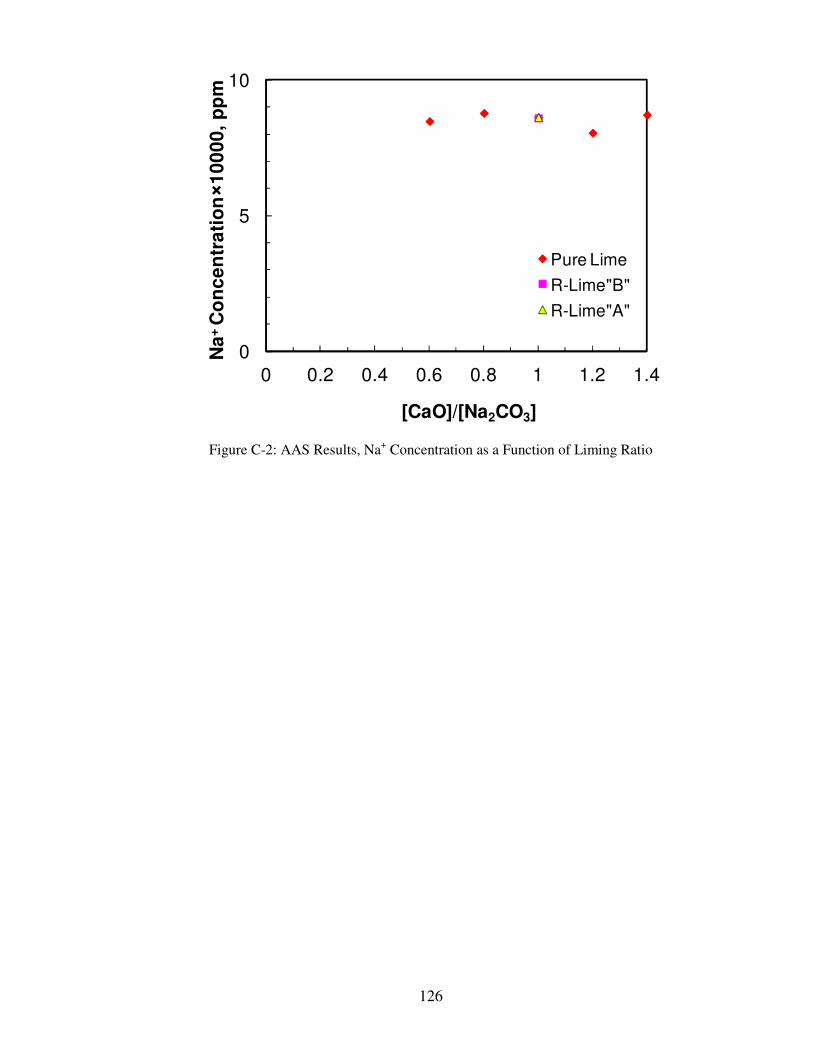
126

Figure C-2: AAS Results, Na+ Concentration as a Function of Liming Ratio

0

5

10

0 0.2 0.4 0.6 0.8 1 1.2 1.4

Pure Lime

R-Lime"B"

R-Lime"A"

Na

+ C

on

ce

ntr

ati

on×

10

00

0,

pp

m

[CaO]/[Na2CO3]

127

Appendix D: Settling Results

Figure D-1: Effect of Liming Ratio on Settling Rate (120 g/L Na2O TTA, and 90 minutes reaction), R-

Lime “A”


Lime “C”

0

5

10

15

20

0 10 20 30 40 50 60

Time, min

Inte

rfa

ce

He

igh

t, c

m

1.2

1

0.7

0.8

0.4

[CaO]/[Na2CO3]=1.4

0.2

0

5

10

15

20

0 30 60 90

Time, min

Inte

rfa

ce

He

igh

t, c

m

[CaO]/[Na2CO3]=1.4

0.6

0.8

1.2

1

128


Lime “D”

0

5

10

15

20

0 10 20 30 40 50 60

Time, min

Inte

rfa

ce

He

igh

t, ,

cm [CaO]/[Na2CO3]=1.4

0.6

0.8

1.2

1

129

Appendix E: Filterability Results

Figure E-1: Effect of Liming Ratio on Filtration Rate (120 g/L Na2O TTA, and 90 minutes reaction, 14

Kilopascal Vacuum), R-Lime “A” using Filterability Set-up Shown in Figure 3-3

Figure E-2: Effect of Liming Ratio on Cake Moisture Content (120 g/L Na2O TTA, and 90 minutes

reaction, 14 Kilopascal Vacuum), R-Lime “A” using Filterability Set-up Shown in Figure 3-3

0

5

10

15

20

0 30 60 90

V, mL

t/v

, S

/mL

[CaO]/[Na2CO3]=1.2

0.520.35

0.15

0.70.6

1 0.85

0.72

30

40

50

60

0.2 0.4 0.6 0.8 1 1.2 1.4

[CaO]/[Na2CO3]

Mo

istu

re C

on

ten

t, %

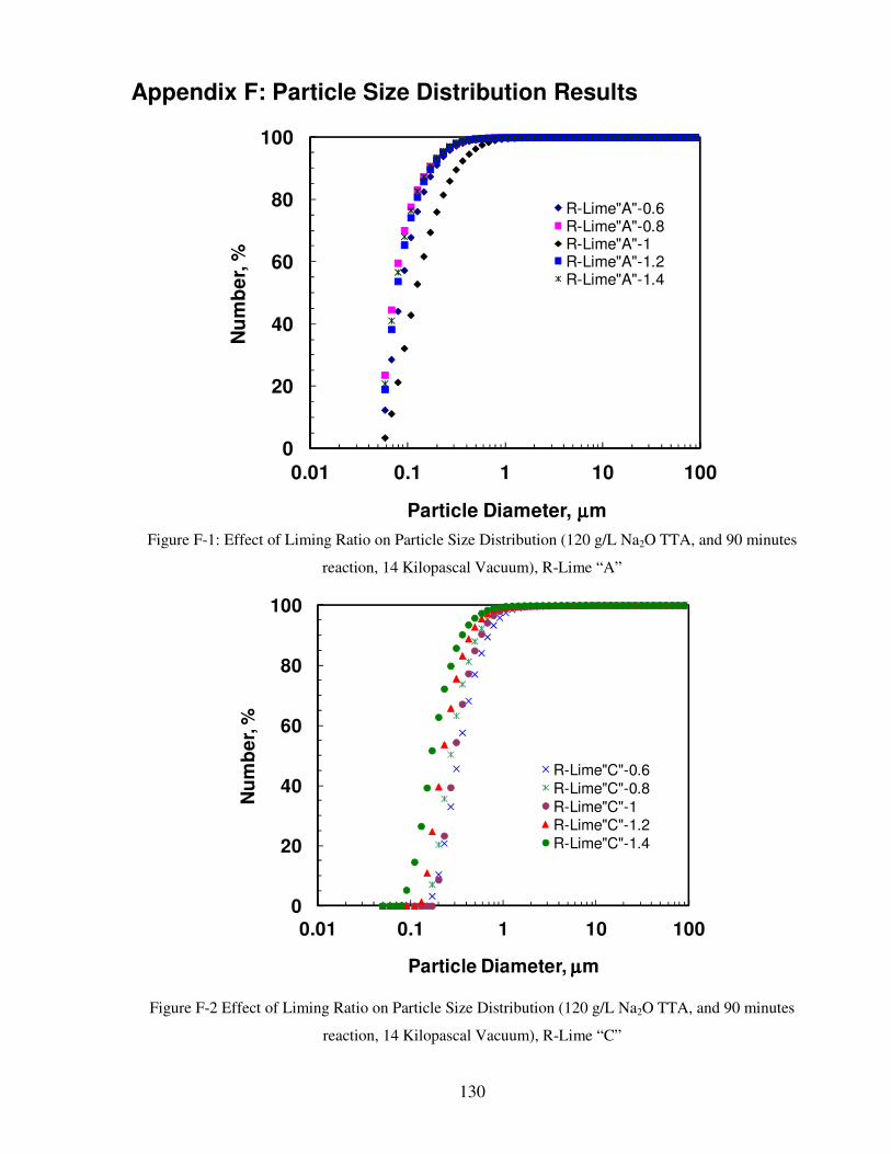
130

Appendix F: Particle Size Distribution Results

Figure F-1: Effect of Liming Ratio on Particle Size Distribution (120 g/L Na2O TTA, and 90 minutes

reaction, 14 Kilopascal Vacuum), R-Lime “A”

Figure F-2 Effect of Liming Ratio on Particle Size Distribution (120 g/L Na2O TTA, and 90 minutes

reaction, 14 Kilopascal Vacuum), R-Lime “C”

0

20

40

60

80

100

0.01 0.1 1 10 100

Nu

mb

er,

%


R-Lime"A"-0.6R-Lime"A"-0.8R-Lime"A"-1R-Lime"A"-1.2R-Lime"A"-1.4

0

20

40

60

80

100

0.01 0.1 1 10 100

Nu

mb

er,

%


R-Lime"C"-0.6

R-Lime"C"-0.8

R-Lime"C"-1R-Lime"C"-1.2

R-Lime"C"-1.4

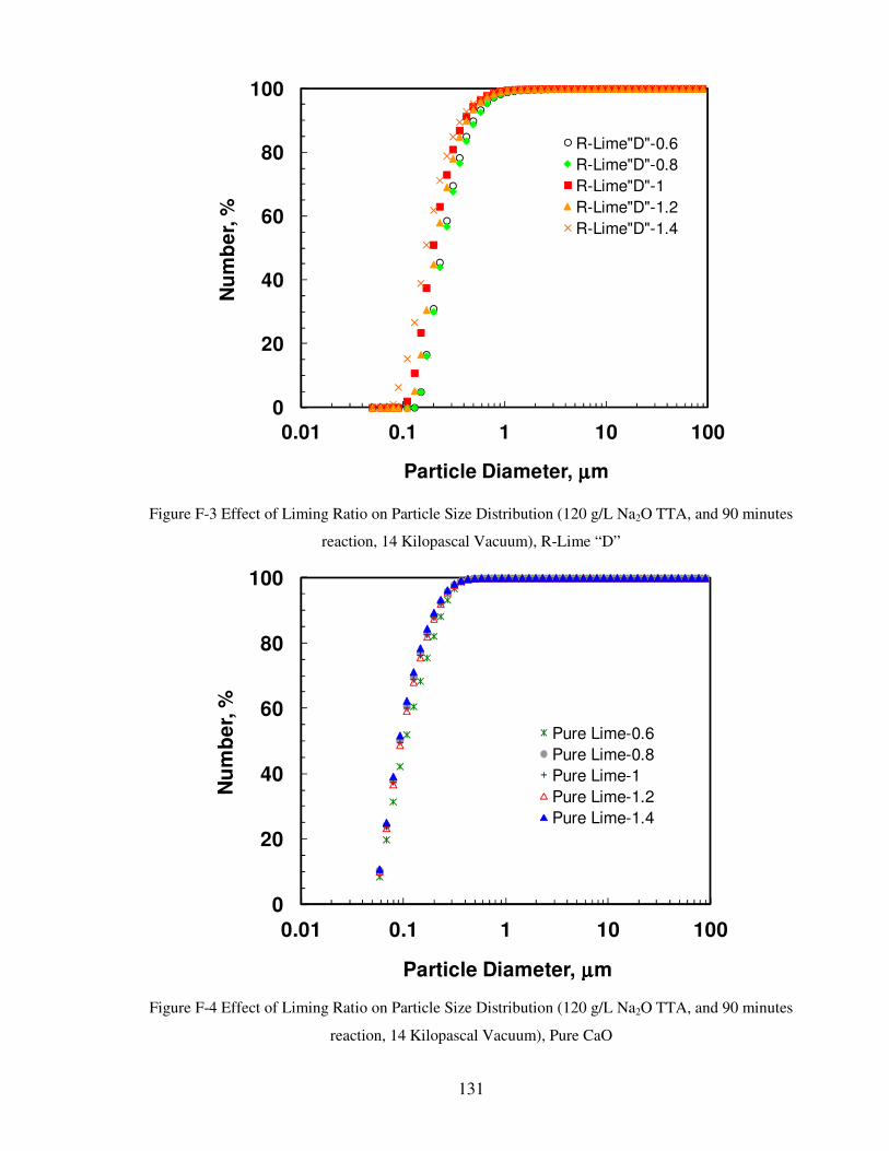
131


reaction, 14 Kilopascal Vacuum), R-Lime “D”


reaction, 14 Kilopascal Vacuum), Pure CaO

0

20

40

60

80

100

0.01 0.1 1 10 100

Nu

mb

er,

%


R-Lime"D"-0.6

R-Lime"D"-0.8

R-Lime"D"-1

R-Lime"D"-1.2

R-Lime"D"-1.4

0

20

40

60

80

100

0.01 0.1 1 10 100

Nu

mb

er,

%


Pure Lime-0.6

Pure Lime-0.8

Pure Lime-1

Pure Lime-1.2

Pure Lime-1.4

132

Appendix G: Liquid Density and Viscosity Measurements

As Figure G-1 and Figure G-2 show liming ratio did not affect liquid (NaOH produced from

reaction of Na2CO3 and CaO) density and viscosity significantly.

Figure G-1 Effect of Liming Ratio on Liquid Density

0

0.2

0.4

0.6

0.8

1

1.2

1.4

0 0.2 0.4 0.6 0.8 1 1.2 1.4

De

ns

ity g

/mL

Pure Lime

R-Lime"B"

R-Lime"A"

[CaO]/[Na2CO3]

133

Figure G-2: Effect of Liming Ratio on Liquid Viscosity

0.0

0.5

1.0

1.5

2.0

2.5

0 0.2 0.4 0.6 0.8 1 1.2 1.4

Vis

co

sit

y, c

p

[CaO]/[Na2CO3]

Pure Lime

R-Lime"A"

R-Lime"B"

134

Appendix H: Effect of Electrolyte Concentration on Settling

Figure H-1 and H-2 show effect of electrolyte (NaCl) concentration on the settling for liming

ratio of 1 and 1.2, respectively. NaCl concentration changed from 0 to 0.1 M. the solid

concentration was 5 wt. %. Results indicate that electrolyte concentration did not affect particle

settling. Since Cl- is indifferent ion and has no special affinity for the surface charge, the settling

did not change and zeta potential may change at very high concentration (5-6 M).

Figure H-1: Effect of Electrolyte Concentration on the Settling (LR=1)

0

2

4

6

8

10

12

14

0 2 4 6 8 10

Time, min

Inte

rfa

ce

He

igh

t, c

m

NaCl 0.1M

NaCl 0.01M

NaCl 0.001M

NaCl 0M

135

Figure H-2: Effect of Electrolyte Concentration on the Settling (LR=1.2)

0

2

4

6

8

10

12

14

0 2 4 6 8 10

Time, min

Inte

rfa

ce

He

igh

t, c

m

NaCl 0.1M

NaCl 0.01M

NaCl 0.001M

NaCl 0M

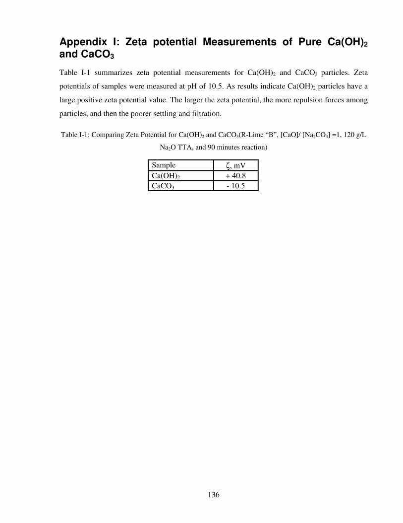
136

Appendix I: Zeta potential Measurements of Pure Ca(OH)2 and CaCO3

Table I-1 summarizes zeta potential measurements for Ca(OH)2 and CaCO3 particles. Zeta

potentials of samples were measured at pH of 10.5. As results indicate Ca(OH)2 particles have a

large positive zeta potential value. The larger the zeta potential, the more repulsion forces among

particles, and then the poorer settling and filtration.

Table I-1: Comparing Zeta Potential for Ca(OH)2 and CaCO3(R-Lime “B”, [CaO]/ [Na2CO3] =1, 120 g/L


Sample ζ, mV

Ca(OH)2 + 40.8

CaCO3 - 10.5

Documents

Impact of Liming Ratio on Lime Mud Settling and Filterability in the