1

Image-Based Sentiment Analysis of Videos

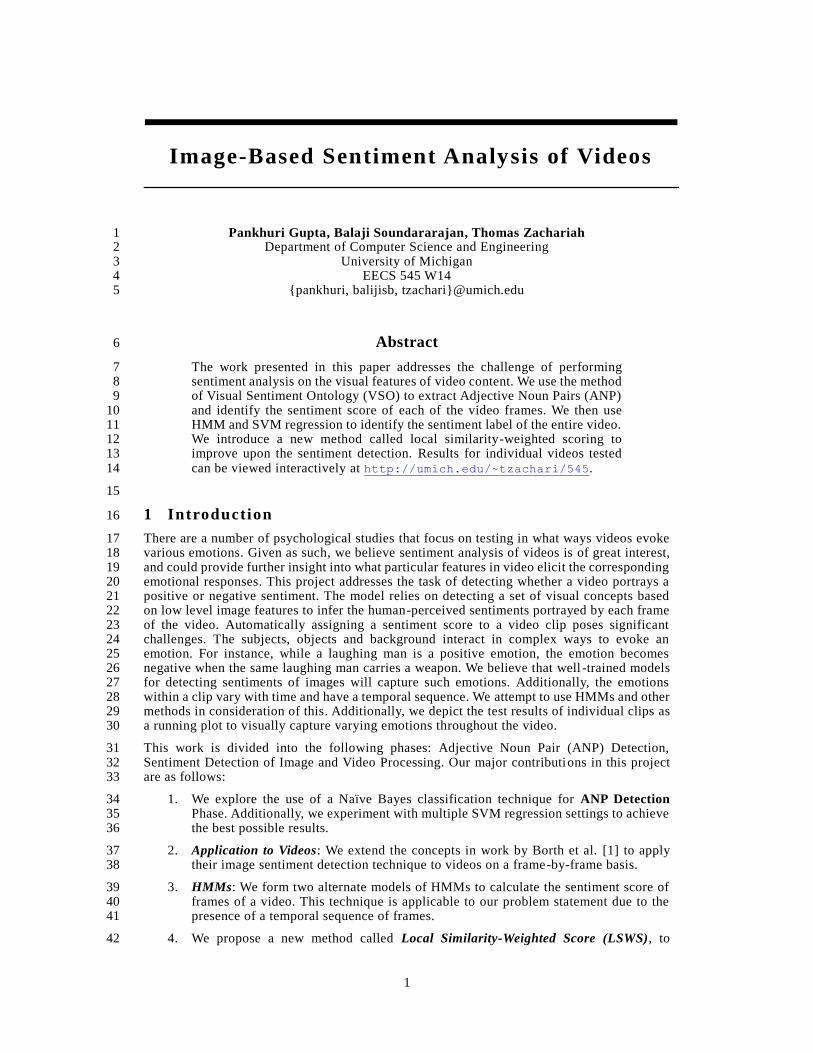
Pankhuri Gupta, Balaji Soundararajan, Thomas Zachariah 1 Department of Computer Science and Engineering 2

University of Michigan 3 EECS 545 W14 4

{pankhuri, balijisb, tzachari}@umich.edu 5

Abstract 6

The work presented in this paper addresses the challenge of performing 7 sentiment analysis on the visual features of video content. We use the method 8 of Visual Sentiment Ontology (VSO) to extract Adjective Noun Pairs (ANP) 9 and identify the sentiment score of each of the video frames. We then use 10 HMM and SVM regression to identify the sentiment label of the entire video. 11 We introduce a new method called local similarity-weighted scoring to 12 improve upon the sentiment detection. Results for individual videos tested 13 can be viewed interactively at http://umich.edu/~tzachari/545. 14

15

1 Introduction 16

There are a number of psychological studies that focus on testing in what ways videos evoke 17 various emotions. Given as such, we believe sentiment analysis of videos is of great interest, 18 and could provide further insight into what particular features in video elicit the corresponding 19 emotional responses. This project addresses the task of detecting whether a video portrays a 20 positive or negative sentiment. The model relies on detecting a set of visual concepts based 21 on low level image features to infer the human-perceived sentiments portrayed by each frame 22 of the video. Automatically assigning a sentiment score to a video clip poses significant 23 challenges. The subjects, objects and background interact in complex ways to evoke an 24 emotion. For instance, while a laughing man is a positive emotion, the emotion becomes 25 negative when the same laughing man carries a weapon. We believe that well -trained models 26 for detecting sentiments of images will capture such emotions. Additionally, the emotions 27 within a clip vary with time and have a temporal sequence. We attempt to use HMMs and other 28 methods in consideration of this. Additionally, we depict the test results of individual clips as 29 a running plot to visually capture varying emotions throughout the video. 30

This work is divided into the following phases: Adjective Noun Pair (ANP) Detection, 31 Sentiment Detection of Image and Video Processing. Our major contributions in this project 32 are as follows: 33

1. We explore the use of a Naïve Bayes classification technique for ANP Detection 34 Phase. Additionally, we experiment with multiple SVM regression settings to achieve 35 the best possible results. 36

2. Application to Videos: We extend the concepts in work by Borth et al. [1] to apply 37 their image sentiment detection technique to videos on a frame-by-frame basis. 38

3. HMMs: We form two alternate models of HMMs to calculate the sentiment score of 39 frames of a video. This technique is applicable to our problem statement due to the 40 presence of a temporal sequence of frames. 41

4. We propose a new method called Local Similarity-Weighted Score (LSWS), to 42

2

improve upon the sentiment scores of images. This method draws on the sequential 43 nature of the frames in a video. 44

5. Web Interface: We present a web interface that gives the entire work that we have done 45 as a part of this project. This interface can be released in the future. 46

47

2 Related Work 48

Sentiment analysis is a widely studied area, however, it has been limited to analysis of text 49 data. Analyzing the sentiments of images is a relatively new field that is gaining more and 50 more popularity with the social web [2] talks about using some very basic visual features and 51 adjectives for finding sentiments portrayed by the images [1] introduces a concept of Adjective 52 noun pairs that offer greater sentiments and uses a richer set of features. They train 1200 53 different binary classifiers (one for each ANP) and pass the test image through each of these 54 classifiers. This gives a 1200 long vector, where each element gives the probability of 55 corresponding ANP occurring in that image. They feed this vector as input to their Sentiment 56 Detector binary classifier that labels the image as +1 or -1(negative). 57

We extend this work by applying the image sentiments to videos. Schaefer et al. [3] and 58 Carvalho et al. [4], from whom we have obtained our testing data (see following section), refer 59 to relatively recent psychophysiological studies on the direct human emotional response to 60 video graphic imagery. Our intent with the application of image sentiment analysis to video, 61 is to take first steps towards developing a model that can generate results comparable to those 62 of such studies and to pinpoint the specific features responsible for various sentiments. 63

Hidden Markov Model assumes that the system is a Markov process with unobserved states. 64 In Bilmes [5], the EM algorithm for HMM with Gaussian Models is described. Though HMMs 65 are applied in temporal pattern recognition [6] such as speech [7], hand-writing etc., they have 66 not been used to model the underlying sentiment of an image. 67

Deep Convolution Neural Networks have been recently shown to yield state -of-the art 68 performance in challenging image classification benchmarks such as ImageNet [8]. While this 69 classification deals with the problem of object recognition, it has not been applied for 70 sentiment analysis. In this project, we have taken a step towards using CNNs for sentiment 71 classification. 72

73

3 Dataset 74

Training ANP Detectors: The binary classifiers for detecting the presence of ANPs within an 75 image are trained and tested using the Flickr Data [9] previously classified by the Visual 76 Sentiment Ontology (VSO) [10]. The training data set comprises about 700 images per ANP. 77 Libsvm’s 5-fold cross validation is used for training purposes and an additional 20% of the 78 data set is held out as validation set. The test data is divided into 5 parts and in total comprises 79 about 300 images. The data sets are balanced and consists of equal number of positive and 80 negative labelled examples. 81

Training Sentiment Binary Classifier: The data set that is used to train and test binary classifier 82 for labelling images as positive and negative sentiment images is a set of 800 Twitter images 83 provided by VSO [10]. This data set has an unequal number of images with negative 84 sentiments. Hence, we have added 400 additional public domain images from Google . 85

Video Dataset: FilmStim database [3] and EMDB database [4] are used for running our models 86 and testing our work. We have received permission for both the datasets to be used for research 87 purposes. 88

Third-party Libraries Utilized: 89

1. The SVM trained binary classifiers for detecting the presence of ANPs in an image as 90 provided by Visual Sentiment Ontology [10]. 91

2. Scikit-learn: A python based library that provides the implementation for Gaussian 92 HMM [11]. 93

3. LibSVM: A Matlab library that implements various settings of a SVM [12]. 94

3

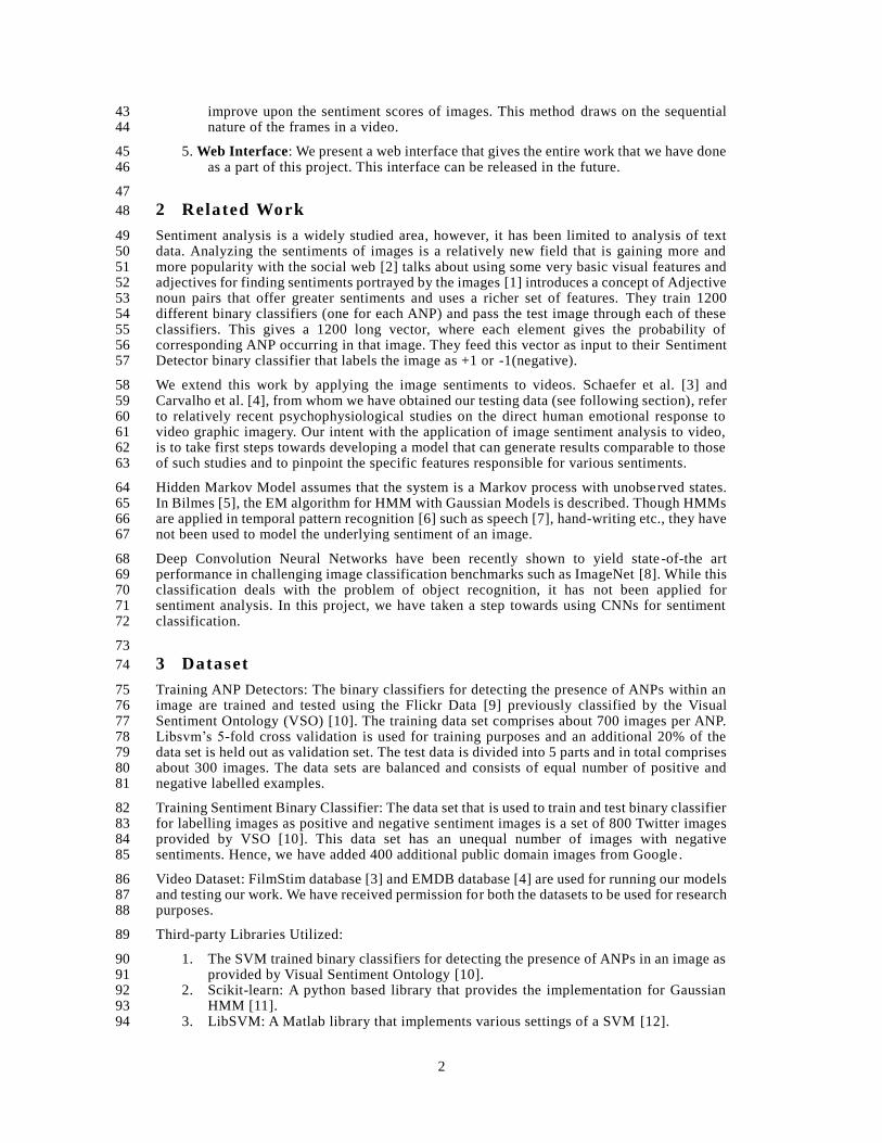
95 Figure 1: Overview of the proposed framework for constructing the visual sentiment ontology, 96

SentiBank and Video Processing. 97

98

4 Methodology 99

The general process framework is depicted in the pipeline shown in Figure 1. The methods 100 that we have utilized throughout the project are discussed in the following subsections. 101

102

4 .1 ANP Detec t io n M ethods 103

104 4 .1 .1 Co mpa r ing M ul t ip le SVM s (Or ig in a l Wo rk ) 105

As mentioned earlier, Borth et al. [1] employs Linear SVM for training the ANP detectors. For 106 each of the 1200 ANPs, they employ a one-vs-all SVM classifier. To compare the accuracy of 107 the different classifiers, we train ANP detectors using different kernel settings for SVM and 108 compare each one to see how the different models behave and perform. The different kernels 109 used are: 110

1. Linear Kernels 111

2. Polynomial Kernels with degree 1 112

3. Polynomial Kernels with degree 2 113

4. RBF kernels 114

5. Sigmoid Kernels 115

For this task, we identify 67 ANPs that best capture the different emotions portrayed by the 116 original 1200 long set and train a classifier for each ANP. 117

118 4 .1 .2 Na ïv e B ay es B ina ry Cla ss i f i er s (Or ig in a l wo r k ) 119

In Borth et al. [1], inputs to the Linear SVMs are different image features like colors (RGB), 120 SIFT or GIST, BOW, LBP, Histogram and PHOW (common descriptors for images). Our 121 assumption is that each of these features capture different properties of the image and are 122 inherently independent. Under this assumption, we test a Naïve Bayes classifier for training 123 ANP detectors for images. Using the same set of 67 ANPs, we compare the rela tive 124 performance of a Naïve Bayes and best SVM classifier. As we discuss in the Experiments 125 section, the Naïve Bayes approach achieves nearly similar accuracy as the best SVM classifier. 126

127

4 .2 Sent i ment Detec t io n M etho ds 128

129

4 .2 .1 SVM Reg ress io n -ba se d Detec t io n 130 (Re - imp lemen ta t io n u s in g S VM in s t ea d o f Lo g is t i c Reg ress io n ) 131

We use a sigmoid kernel SVM regression to find the sentiment score of an image. The feature 132 set for this system is the output from the ANP detection phase in the form of a 708 long vector 133 containing the probabilities of that ANP belonging to the image, scaled by the individual 134 sentiment score of the ANP. Borth et al. [1] uses Logistic Regression for this purpose. 135

4

4 .2 .2 Co nv o lut io n Neura l Netw o rks (O r ig in a l wo r k ) 136

The Convolution Neural Networks have been proven to produce very good results in image 137 segmentation and object detection. We attempt to extend the use of CNNs to use it for ANP 138 detection and sentiment label of the image. We use the Deep Learning Toolbox for MATLAB 139 to implement a 6 layered CNN (3 convolution layers and 3 sub sampling layers). 140

141 4 .3 Sent i ment Ana ly s i s o f Video s (O r ig in a l wo rk ) 142

In this project, we are interested in examining the feasibility and relative accuracy of applying 143 a trained photograph-based image sentiment analysis model such as our own to videos as a 144 method of identifying the graphical features in film that illicit psychophysiological responses 145 so as to classify the expected positive or negative emotional response in humans. 146

To this end, we use 34 film clips from the FilmStim database [3] as the test set. Each clip in 147 this database is affiliated with an emotion such as sadness, anger, amusement or disgust, which 148 was assigned during an associated study in which emotional responses of humans were 149 recorded during in-lab viewings. In order to prepare the data for efficient and adequate 150 analysis, we have sampled each clip at one frame per second. 151

The different methods that we have employed to perform sentiment analysis on video are: 152

1. Linear SVM — We parse each frame individually through our pipeline to extract the 153 sentiment score and produce an effective ‘mapping of the sentiment’ for each of the 154 34 clips to plot the time variation of the sentiment across the clips. This, as expected, 155 yields a certain degree of mixed results. However, we do find that the model is capable 156 of picking up on changes in trends of similar cinematic compositions. In the end, 157 sentiment scores of each sample snapshot is averaged to provide the final score for 158 the video. 159

2. HMM-1 — We believe that the sentiment scores of each frame should have temporal 160 correlation. Usually, an event spans across continuous frames, which should lead to 161 these frames having similar sentiment scores. With this underlying assumption, we 162 use the uncorrelated sentiment score of individual frames to find the hidden correlated 163 sentiment labels of each frame. 164

3. HMM-708 — Instead of using the sentiment scores as the observations, we directly 165 take the ANP probability scores as the observations. We assume that the ANP scores 166 follow a Gaussian distribution and use a discrete state HMM with Gaussian 167 observations. The hidden state describes the sentiment label of the frames. 168

4. Local Similarity Weighted SVM (LSWS) — We propose a new method to revise the 169 sentiment scores of the video frames. We revise the sentiment score of each frame 170 obtained from the SVM regression, using the scores of its neighboring frames. These 171 scores are weighted according to a) the cosine similarity and b) the time lag between the 172 frame under reference and its corresponding neighbors. The number of neighboring frames 173 that are taken into consideration while revising the sentiment score of the particular frame 174 is controlled by a factor “τ” called the field width. Time lag refers to the difference between 175 the timestamp of the frames. For instance, if, say, frame number 15 is being processed, its 176 immediate neighbors 14 and 16 will have time difference of 1. Equation 1 depicts how to 177 calculate this score. 178

(1)

179 180

5

5 Experiments and Results 181

182

5 .1 ANP Detec t io n Pha se 183

184

5 .1 .1 Comparing Different SVMs 185

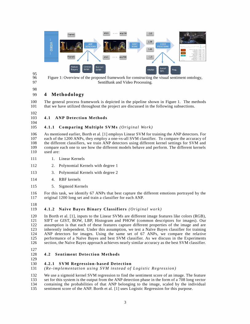
We compare different SVM kernels based upon the accuracy achieved by each on the test set. 186 It is observed that across all ANPs, the sigmoid kernels consistently give the worst 187 performance. The performance of other SVM settings are similar to each other. Figure 2 shows 188 percent accuracies of these different settings. The graph also depicts the best SVM setting 189 selected for each ANP to give the final trained model (red line). 190

191

192

Figure 2: Comparison of 67 ANPs for 6 different kernel settings for SVM classification. The 193 accuracies have been computed by average of runs over 5 different test sets. The best performing 194

kernel for each ANP is shown by the red plot. 195

196

5 .1 .2 Naïve Bayes vs. SVM 197

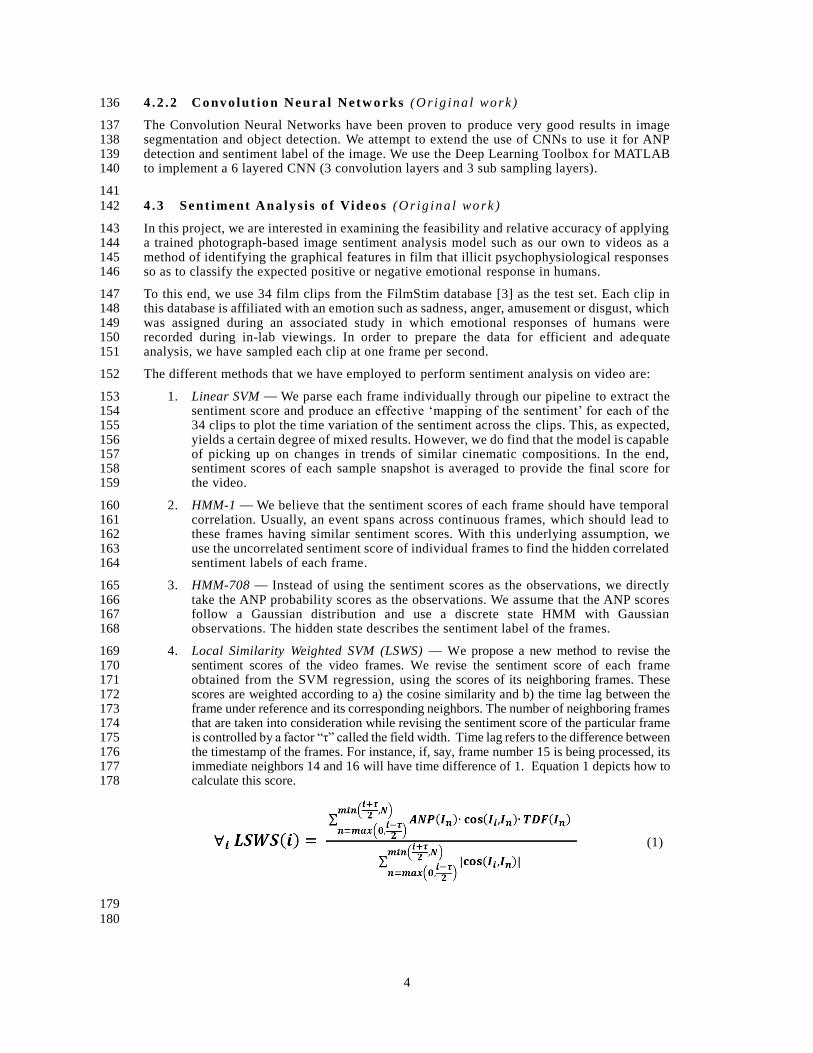
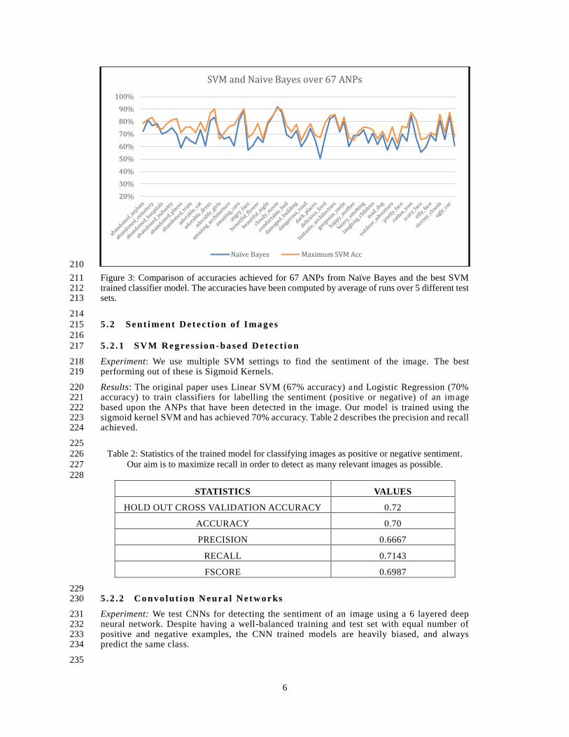
We draw a comparison between the binary classifiers for detecting the presence of ANPs in an 198 image trained using Naïve Bayes and the best SVM binary classifier. Figure 3 shows the 199 percent accuracies achieved for all the ANPs. It is observed that although the overall winner 200 is SVM, however, Naïve Bayes classifiers do not lag behind with a huge margin. The 201 difference however, is huge in terms of the time taken to train each classifier. Table 1 shows 202 the average time taken to train a Naïve Bayes and a SVM classifier. Hence, we see that a 203 relatively simpler model (Naïve Bayes) performance is close to the complex SVM model 204 yielding a huge time benefit. 205

206 Table 1: Average time taken per ANP to train a binary classifier 207

208

AVERAGE TIME TAKEN per ANP (in seconds)

NAÏVE BAYES SVM

1.42334 52.35

209

20%

30%

40%

50%

60%

70%

80%

90%

100%

Accuracies of LibSVM Models over 67 ANPs

-t 0' -t 1 -d 1 -g 0.5' -t 1 -d 2 -r 0.5 -g 1 -t 2 -g 0.5

-t 2 -g 0.6 -t 3 Maximum SVM Acc

6

210

Figure 3: Comparison of accuracies achieved for 67 ANPs from Naïve Bayes and the best SVM 211 trained classifier model. The accuracies have been computed by average of runs over 5 different test 212 sets. 213

214

5 .2 Sent i ment Detec t io n o f I ma g es 215

216

5 .2 .1 SVM Reg ress io n -ba se d Detec t io n 217

Experiment: We use multiple SVM settings to find the sentiment of the image. The best 218 performing out of these is Sigmoid Kernels. 219

Results: The original paper uses Linear SVM (67% accuracy) and Logistic Regression (70% 220 accuracy) to train classifiers for labelling the sentiment (positive or negative) of an image 221 based upon the ANPs that have been detected in the image. Our model is trained using the 222 sigmoid kernel SVM and has achieved 70% accuracy. Table 2 describes the precision and recall 223 achieved. 224

225

Table 2: Statistics of the trained model for classifying images as positive or negative sentiment. 226

Our aim is to maximize recall in order to detect as many relevant images as possible. 227

228

STATISTICS VALUES

HOLD OUT CROSS VALIDATION ACCURACY 0.72

ACCURACY 0.70

PRECISION 0.6667

RECALL 0.7143

FSCORE 0.6987

229 5 .2 .2 Co nv o lut io n Neura l Netw o rks 230

Experiment: We test CNNs for detecting the sentiment of an image using a 6 layered deep 231 neural network. Despite having a well-balanced training and test set with equal number of 232 positive and negative examples, the CNN trained models are heavily biased, and always 233 predict the same class. 234

235

20%

30%

40%

50%

60%

70%

80%

90%

100%

SVM and Naive Bayes over 67 ANPs

Naïve Bayes Maximum SVM Acc

7

Analysis: The data set we use for training the CNN models is the set of labeled images from 236 Twitter as provided by [1]. As this is a very small data set (comprising about 1000 images), 237 the resulting train and test set is very limited. Additional fine tuning of the initial parameters 238 is required for CNNs to ensure that they do not get trapped in local minima. 239

240

5 .3 Sent i ment Ana ly s i s o f Video s 241

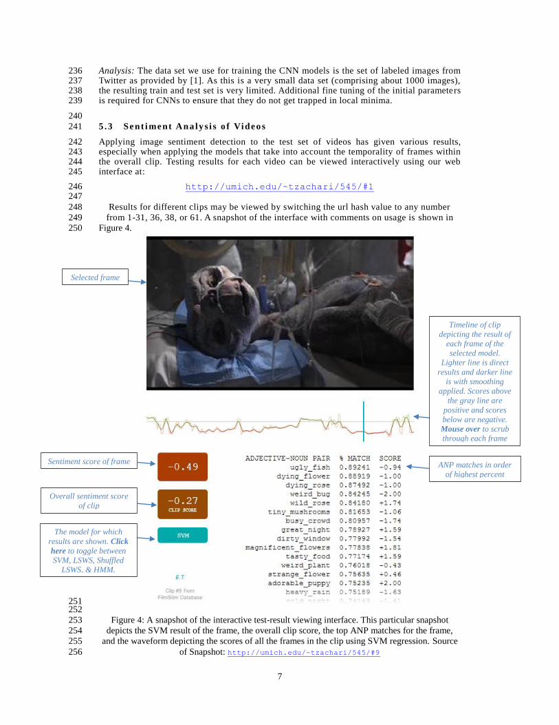
Applying image sentiment detection to the test set of videos has given various results, 242 especially when applying the models that take into account the temporality of frames within 243 the overall clip. Testing results for each video can be viewed interactively using our web 244 interface at: 245

http://umich.edu/~tzachari/545/#1 246 247

Results for different clips may be viewed by switching the url hash value to any number 248

from 1-31, 36, 38, or 61. A snapshot of the interface with comments on usage is shown in 249

Figure 4. 250

251 252

Figure 4: A snapshot of the interactive test-result viewing interface. This particular snapshot 253

depicts the SVM result of the frame, the overall clip score, the top ANP matches for the frame, 254

and the waveform depicting the scores of all the frames in the clip using SVM regression. Source 255

of Snapshot: http://umich.edu/~tzachari/545/#9 256

Sentiment score of frame

Overall sentiment score

of clip

The model for which

results are shown. Click

here to toggle between

SVM, LSWS, Shuffled

LSWS, & HMM.

ANP matches in order

of highest percent

match

Timeline of clip

depicting the result of

each frame of the

selected model.

Lighter line is direct

results and darker line

is with smoothing

applied. Scores above

the gray line are

positive and scores

below are negative.

Mouse over to scrub

through each frame

Selected frame

8

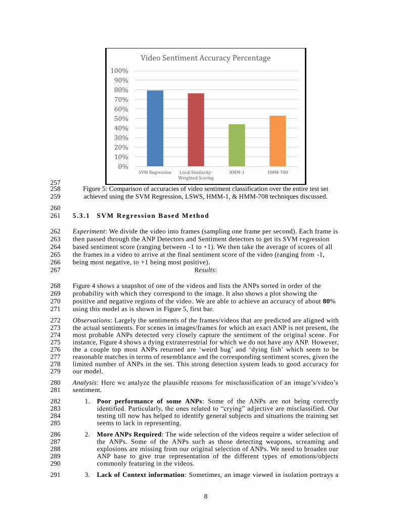
257 Figure 5: Comparison of accuracies of video sentiment classification over the entire test set 258

achieved using the SVM Regression, LSWS, HMM-1, & HMM-708 techniques discussed. 259

260

5 .3 .1 SVM Reg ress io n B a sed M etho d 261

Experiment: We divide the video into frames (sampling one frame per second). Each frame is 262

then passed through the ANP Detectors and Sentiment detectors to get its SVM regression 263

based sentiment score (ranging between -1 to +1). We then take the average of scores of all 264

the frames in a video to arrive at the final sentiment score of the video (ranging from -1, 265

being most negative, to +1 being most positive). 266

Results: 267

Figure 4 shows a snapshot of one of the videos and lists the ANPs sorted in order of the 268

probability with which they correspond to the image. It also shows a plot showing the 269

positive and negative regions of the video. We are able to achieve an accuracy of about 80% 270

using this model as is shown in Figure 5, first bar. 271

Observations: Largely the sentiments of the frames/videos that are predicted are aligned with 272 the actual sentiments. For scenes in images/frames for which an exact ANP is not present, the 273 most probable ANPs detected very closely capture the sentiment of the origina l scene. For 274 instance, Figure 4 shows a dying extraterrestrial for which we do not have any ANP. However, 275 the a couple top most ANPs returned are ‘weird bug’ and ‘dying fish’ which seem to be 276 reasonable matches in terms of resemblance and the corresponding sentiment scores, given the 277 limited number of ANPs in the set. This strong detection system leads to good accuracy for 278 our model. 279

Analysis: Here we analyze the plausible reasons for misclassification of an image’s/video’s 280 sentiment. 281

1. Poor performance of some ANPs: Some of the ANPs are not being correctly 282 identified. Particularly, the ones related to “crying” ad jective are misclassified. Our 283 testing till now has helped to identify general subjects and situations the training set 284 seems to lack in representing. 285

2. More ANPs Required: The wide selection of the videos require a wider selection of 286 the ANPs. Some of the ANPs such as those detecting weapons, screaming and 287 explosions are missing from our original selection of ANPs. We need to broaden our 288 ANP base to give true representation of the different types of emotions/objects 289 commonly featuring in the videos. 290

3. Lack of Context information: Sometimes, an image viewed in isolation portrays a 291

0%

10%

20%

30%

40%

50%

60%

70%

80%

90%

100%

SVM Regression Local Similarity-Weighted Scoring

HMM-1 HMM-708

Video Sentiment Accuracy Percentage

9

different meaning than when it is part of a complete video. As our method views 292 snapshots in isolation and does not have any information about the context of the 293 video, it results in labelling positive images as negative or vice versa. For instance, 294 one of the videos in our data set shows scenes from a dry comedy in which most of 295 the individual frames are wrongly labeled as negative. 296

297 5 .3 .2 HM M Resul t s 298

Experiment: We use the Gaussian HMM implementation of python-sklearn to learn a first 299 order HMM with discrete hidden states (possible values: +1, -1). The implementation we call 300 HMM-1 uses one-dimensional observations (the uncorrelated SVM regression sentiment 301 scores of the frame) and implementation HMM-708 uses the multi-dimensional observations 302 (probability scores of each of the 708 ANPs for the frame obtained from the ANP Detection 303 phase). For both implementations, expectation maximization is executed for approximately 304 100 iterations and then Viterbi algorithm is applied to find the best possible state sequence. 305 We run different trials for the HMMs and picks the model corresponding to the maximum log 306 probability score. This initializes the training system with random values and hence ensures 307 that we are not actually selecting a local minima. 308

Observations: Contrary to our initial expectations, the HMMs have performed poorer than 309 SVM, achieving only about 44% and 50% accuracy (Figure 5 third and fourth bar respectively). 310 HMM-708 performed slightly better than HMM-1. This is as expected and thereby 311 corroborates the correlation between the visual concepts (ANPs) and the sentiment of the 312 frame. 313

Analysis: 314

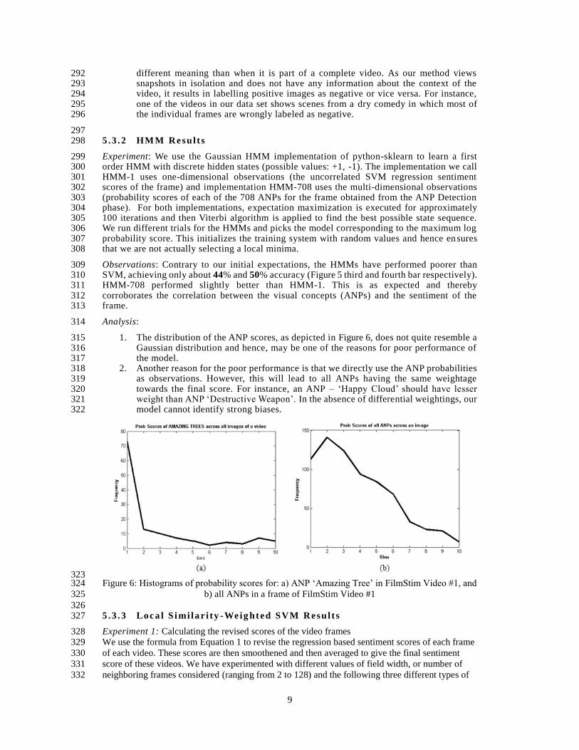
1. The distribution of the ANP scores, as depicted in Figure 6, does not quite resemble a 315 Gaussian distribution and hence, may be one of the reasons for poor performance of 316 the model. 317

2. Another reason for the poor performance is that we directly use the ANP probabilities 318 as observations. However, this will lead to all ANPs having the same weightage 319 towards the final score. For instance, an ANP – ‘Happy Cloud’ should have lesser 320 weight than ANP ‘Destructive Weapon’. In the absence of differential weightings, our 321 model cannot identify strong biases. 322

323 Figure 6: Histograms of probability scores for: a) ANP ‘Amazing Tree’ in FilmStim Video #1, and 324

b) all ANPs in a frame of FilmStim Video #1 325

326 5 .3 .3 Lo ca l S i mi la r i ty -Weig hted SVM Resu l t s 327

Experiment 1: Calculating the revised scores of the video frames 328 We use the formula from Equation 1 to revise the regression based sentiment scores of each frame 329

of each video. These scores are then smoothened and then averaged to give the final sentiment 330

score of these videos. We have experimented with different values of field width, or number of 331

neighboring frames considered (ranging from 2 to 128) and the following three different types of 332

10

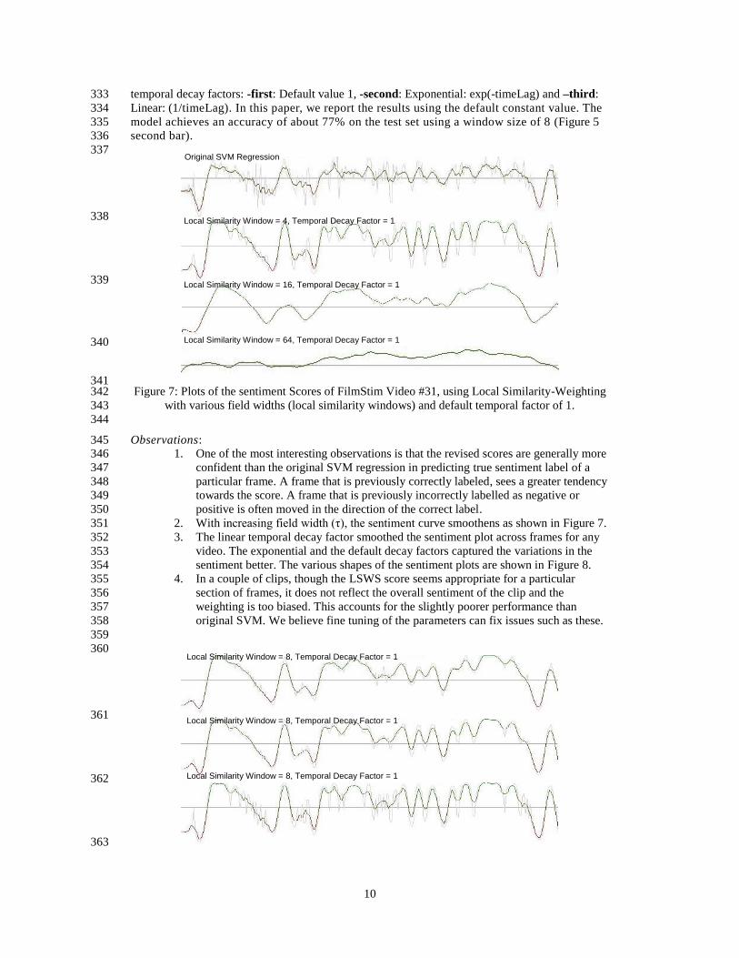
temporal decay factors: -first: Default value 1, -second: Exponential: exp(-timeLag) and –third: 333

Linear: (1/timeLag). In this paper, we report the results using the default constant value. The 334

model achieves an accuracy of about 77% on the test set using a window size of 8 (Figure 5 335

second bar). 336

337

338

339

340

341 Figure 7: Plots of the sentiment Scores of FilmStim Video #31, using Local Similarity-Weighting 342

with various field widths (local similarity windows) and default temporal factor of 1. 343

344

Observations: 345 1. One of the most interesting observations is that the revised scores are generally more 346

confident than the original SVM regression in predicting true sentiment label of a 347

particular frame. A frame that is previously correctly labeled, sees a greater tendency 348

towards the score. A frame that is previously incorrectly labelled as negative or 349

positive is often moved in the direction of the correct label. 350

2. With increasing field width (τ), the sentiment curve smoothens as shown in Figure 7. 351

3. The linear temporal decay factor smoothed the sentiment plot across frames for any 352

video. The exponential and the default decay factors captured the variations in the 353

sentiment better. The various shapes of the sentiment plots are shown in Figure 8. 354

4. In a couple of clips, though the LSWS score seems appropriate for a particular 355

section of frames, it does not reflect the overall sentiment of the clip and the 356

weighting is too biased. This accounts for the slightly poorer performance than 357

original SVM. We believe fine tuning of the parameters can fix issues such as these. 358

359

360

361

362

363

Original SVM Regression

Local Similarity Window = 4, Temporal Decay Factor = 1

Local Similarity Window = 16, Temporal Decay Factor = 1

Local Similarity Window = 64, Temporal Decay Factor = 1

Local Similarity Window = 8, Temporal Decay Factor = 1

Local Similarity Window = 8, Temporal Decay Factor = 1

Local Similarity Window = 8, Temporal Decay Factor = 1

11

Figure 8: Plots of the sentiment scores of FilmStim Video #31, using Local Similarity-Weighting 364

with various temporal factors and similarity window of 8. 365

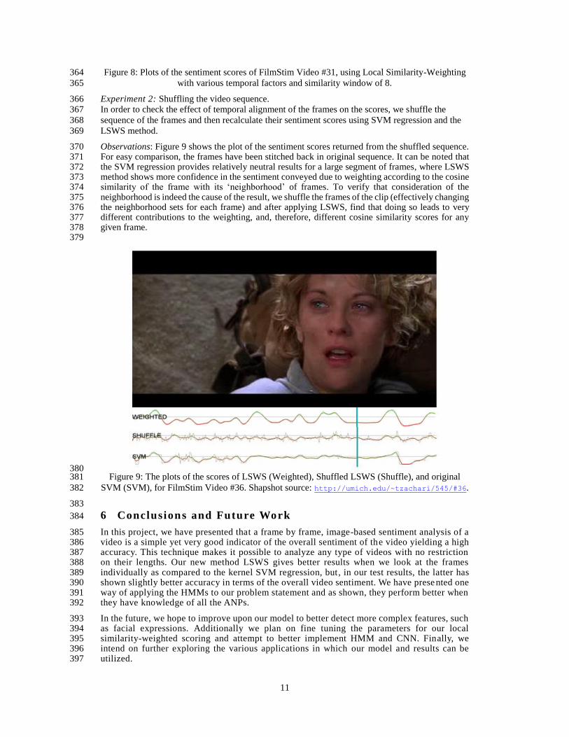
Experiment 2: Shuffling the video sequence. 366 In order to check the effect of temporal alignment of the frames on the scores, we shuffle the 367

sequence of the frames and then recalculate their sentiment scores using SVM regression and the 368

LSWS method. 369

Observations: Figure 9 shows the plot of the sentiment scores returned from the shuffled sequence. 370 For easy comparison, the frames have been stitched back in original sequence. It can be noted that 371 the SVM regression provides relatively neutral results for a large segment of frames, where LSWS 372 method shows more confidence in the sentiment conveyed due to weighting according to the cosine 373 similarity of the frame with its ‘neighborhood’ of frames. To verify that consideration of the 374 neighborhood is indeed the cause of the result, we shuffle the frames of the clip (effectively changing 375 the neighborhood sets for each frame) and after applying LSWS, find that doing so leads to very 376 different contributions to the weighting, and, therefore, different cosine similarity scores for any 377 given frame. 378 379

380 Figure 9: The plots of the scores of LSWS (Weighted), Shuffled LSWS (Shuffle), and original 381

SVM (SVM), for FilmStim Video #36. Shapshot source: http://umich.edu/~tzachari/545/#36. 382

383

6 Conclusions and Future Work 384

In this project, we have presented that a frame by frame, image-based sentiment analysis of a 385 video is a simple yet very good indicator of the overall sentiment of the video yielding a high 386 accuracy. This technique makes it possible to analyze any type of videos with no restriction 387 on their lengths. Our new method LSWS gives better results when we look at the frames 388 individually as compared to the kernel SVM regression, but, in our test results, the latter has 389 shown slightly better accuracy in terms of the overall video sentiment. We have prese nted one 390 way of applying the HMMs to our problem statement and as shown, they perform better when 391 they have knowledge of all the ANPs. 392

In the future, we hope to improve upon our model to better detect more complex features, such 393 as facial expressions. Additionally we plan on fine tuning the parameters for our local 394 similarity-weighted scoring and attempt to better implement HMM and CNN. Finally, we 395 intend on further exploring the various applications in which our model and results can be 396 utilized. 397

12

398

Ac kno w ledg me nts 399

We would first like to thank Professor Satinder Baveja for his help and motivation in pursuing 400 this project. Additionally, we would like to acknowledge Borth et al. [1], Schaefer et al. [3], 401 and Carvalho et al. [4], all of whose studies and corresponding datasets have played a large 402 part in our project. We have used MATLAB and Python for all programming that necessary 403 for this project. 404

405

References 406

[1] D. Borth, R. Ji, T. Chen, T. Breuel and S.-F. Chang, "Large-scale Visual Sentiment

Ontology and Detectors Using Adjective Noun Pairs," in ACM Int. Conference on

Multimedia (ACM MM), Barcelona, Spain, 2013.

[2] S. Siersdorfer and J. Hare, "Analyzing and Predicting Sentiment of Images on the Social

Web," ACM, 2010.

[3] A. Schaefer, F. Nils, X. Sanchez and P. Philippot, "Assessing the Effectiveness of a Large

Database of Emotion-eliciting Films: A New Tool for Emotion Researchers," Cognition &

Emotion, vol. 24, no. 7, pp. 1153-1172, 2010.

[4] S. Carvalho, J. Leite, S. Galdo-Álvarez and Ó. F. Gonçalves, "The Emotional Movie

Database (EMDB): A Self-Report and Psychophysiological Study," Applied

Psychophysiology and Biofeedback, vol. 37, no. 4, pp. 279-94, 2012.

[5] J. A. Bilmes, "A Gentle Tutorial of the EM Algorithm and its Application to Parameter

Estimation for Gaussian Mixture and Hidden Markov Models," 1998.

[6] B. C. Lovell, "Hidden Markov Models for Spatio-Temporal Pattern Recognition and Image

Segmentation," in International Conference on Advances in Pattern Recognition, Kolkatta,

2003.

[7] D. Paul, "Speech Recognition Using Hidden Markov Models," Lincoln Laboratory Journal ,

vol. 3, no. 1, 1990.

[8] A. Krizhevsky, I. Sutskever and G. Hilton, "ImageNet Classification with Deep Convolution

Neural Networks," NIPS, pp. 1106-1114, 2012.

[9] "Flickr API," [Online]. Available: http://www.flickr.com/services/api.

[10] "Visual Sentiment Ontology," [Online]. Available: http://visual-sentiment-

ontology.appspot.com.

[11] Scikit-Learn. [Online]. Available: http://scikit-

learn.org/stable/modules/generated/sklearn.hmm.GaussianHMM.html.

[12] "LibSVM," [Online]. Available: www.csie.ntu.edu.tw/~cjlin/libsvm/.

407

408