Embed Size (px)
Citation preview
Spectroscopy of ultracold metastable hydrogen: in
pursuit of a precision measurement
by
Kendra Margaret Denny Vant
Submitted to the Department of Physics in partial fulfillment of the requirements for the degree of
Doctor of Philosophy
at the
MASSACHUSETTS INSTITUTE OF TECHNOLOGY @ePlefn+m wcj3
June 2005
@ Kerldra Margaret Denny Vant, MMV. All rights reserved.
The autlhor hereby grants to MIT permission to reproduce and distribute publicly paper and electronic copies of this thesis document
ARCHIVES
in whole or in part. MASSACHUSETTS I N ~ E '
- -. /" . . .
OF TECHNOLOGY
LIBRARIES Author . . . . . . . . . . . . . . . . . . . . . . . . . . . .- - &../ . . . . . . . . . . . . . . . . . . . . . . I
Department of Physics 8 June, 2005
Certified b y ........................ .w+.-r. . . . . . . . . . . . . . . aniel Kleppner
Lester Wolfe Professor of Physics - - Thesis Supervisor, ,
Certified by. - . . . . . . . . . . . . . . . . . . . . . . . . . . . . . .
ofessor ihomasPak - Thegis Supervisor,
?
Accepted by . . . . . . . . . . . . . . . . . . . . . . . . . . . I'
k ' h o m a s p a k " Chairman, Department ofphysics GraduateC mittee

Spectroscopy of ultracold metastable hydrogen: in pursuit of
a precision measurement
Kendra Margaret Denny Vant
Submitted to the Department of Physics on 8 June, 2005, in partial fulfillment of the
requirements for the degree of Doctor of Philosophy
Abstract
This thesis describes the first observations in trapped hydrogen of optical transitions starting from the metastable 2s state. It covers in detail the design and construction of two stabilized diode laser systems for performing spectroscopy of the 2s-3P and 2s-8s transitions.
Spectroscopy of the one photon 2s-3P transition in hydrogen is demonstrated both by the depletion of the metastable 2 s atom state and the absorption of the 2s-3P laser light. A model for absorption spectroscopy as a probe for metastable number is developed and absorption is shown to offer a major improvement over current detection methods. In the course of these experiments, techniques with diode lasers were developed that will be used later in the proposed precision measurements of 2s-nS transitions.
The design, construction and characterization of the diode laser system for per- forming spectroscopy of the two photon 2s-8s transition is explained and recom- mended parameters for a proposed signal search are outlined.
Thesis Supervisor: Daniel Kleppner Title: Lester Wolfe Professor of Physics
Thesis Supervisor: Thomas Greytak Title: Professor

Acknowledgments
So very many people have supported, encouraged and inspired me during my six years
at MIT that I can only do justice to a few here. The rest will live on in my heart and
my memories.
To begin I would like to thank my advisors, Dan Kleppner and Tom Greytak. The
Ultracold Hydrogen lab is an enduring symbol of their dedication and commitment
to basic scientific research even when times are slow and the experiments are tough.
I have learned much from Tom and Dan that I will carry with me in the years to
come.
Dave Pritchard has been a supportive and engaged academic advisor from day
one. I will always remember Eric Hudson for his approachability and his personal
concern.
Julia Steinberger welcomed me into the lab and into her life. Over five years
together in the lab, we developed an enduring friendship and had a lot of laughs.
Greg and I will always remember the warmth and generosity with which Julia shared
her family. She seemed to understand as few others did, how much we missed New
Zealand in the early years.
I enjoyed sharing the lab for four years with Lorenz Willmann. While things didn't
always go according to plan, mine or his, we got stuff done and had some great times
along the way.
Cort and Corey Johnson arrived in lab life in 2001 when Cort joined the Ultracold
Hydrogen group as a first year graduate student. I count their friendship as one of
the high points of my time at MIT. Cort's calm and measured presence in the lab
and his quiet humor were a wonderful addition to our highly strung team. I would
also like to pa,rticularly thank Cort for his prompt, thorough and critical reading of
this thesis.
Lia Matos ha,s been a great colleague and an even better friend. With her, more
than anyone, I share both the sorrow of an experiment that could not be bought to
fruition and the joy of our laser physics achievements. Over the years, we negotiated
courses, qualifying exams, research woes and (wonderfully) motherhood in tandem.
She, Pedro and Clara will always hold a special place in my heart. Tycho will miss
his little sister so much.
In the past couple of years, it has been a lot of fun to have Rob decarvalho,
Bonna Newman and Nathan Brahms around the lab. I have enjoyed sharing in Rob's
crazy physics ideas and expect to see some important patents being developed in near
future.
All the inhabitants of the second floor of Building 13 have contributed in their
own ways to the richness of my time at MIT. I particularly enjoyed sharing in the
mini baby boom of 2003-2004.
I would like to acknowledge both Mary Rowe and Blanche Staton for providing
a ready ear and sound advice in a time of need and Miriam Kahn for four years of
patient and unwavering support.
My sister in law, Katherine Ball, has provided an oasis of calm and non-physics
related conversation during these last busy weeks. Greg, Tycho and I will always be
indebted to her for her love and support.
Gillian Paku and family have helped us recreate a little home-away-from-home
here in Boston. We have very deeply appreciated all the support and good food they
have provided and look forward to continuing the friendship when we all finally return
to home shores.
Throughout my time at MIT, I have thoroughly enjoyed participating in the Grad-
uate Women in Physics Group. Wphys has provided me the opportunity to meet and
get to know many interesting people from all flavors of physics, an experience to be
treasured in a department as large as this one.
Gary Steele and Oliver Dial of the Ashoori Group were always ready to share
their expertise in the realms of computing and electronics. Many a time, a seeming
insurmountable problem has been overcome with their cheerful and seemingly limitless
assistance.
From the very beginnings of my life, I have been supported by my parents Anne
Denny and Robin Vant. I cherish the family life they created and will never cease

to benefit from the spirit of inquiry and joy in learning that they nurtured. Many
thanks are also due to my sister Arwen and brother Murdoch. None of you may really
understand wh.y I have persisted so long in banging my head against this brick wall
called physics but you have always been wonderfully non-judgemental!
Finally I would like to acknowledge, at least to the extent that words can, the fun-
damental, sustaining support of my husband Greg Ball. In our eleven years together,
we have built a relationship strong enough to withstand not just one PhD but two!
Our growing fa,mily has filled my life with a joy and purpose like none other. I look
forward to a lifetime of love where ever life may take us now.

Contents
1 Introduction
2 Ultracold Hydrogen
2.1 Trapping and cooling of 1s hydrogen . . . . . . . . . . . . . . . . . .
. . . . . . . . . . . . . . . . . . . . . . . . . 2.2 2s hydrogen production
. . . . . . . . . . . . . . . . . . . . . . . . . . 2.3 2s hydrogen detection
2.4 2s signal - Doppler free and Doppler sensitive . . . . . . . . . . . . .
. . . . . . . . . . . . . . . . . . . . . . . . . . . 2.5 2s sample parameters
3 Diode Lasers: properties and stabilization schemes
. . . . . . . . . . . . . . . . . . . . . . . . . . . . . . 3.1 Diode structure
. . . . . . . . . . . . . . . . . . . . . . . . . . 3.2 Tuning characteristics
. . . . . . . . . . . . . . . . . . . . . . 3.3 Grating feedback stabilization
3.4 Passive frequency stabilization . . . . . . . . . . . . . . . . . . . . . .
. . . . . . . . . . . . . . . . . . . . . . . . . . . . 3.5 Operational quirks
3.6 Diode lasers for 2s-3P spectroscopy . . . . . . . . . . . . . . . . . . .
3.7 Diode lasers for 2s-8s spectroscopy . . . . . . . . . . . . . . . . . . .
4 Iodine Frequency Reference
. . . . . . . . . 4.1 Saturated absorption spectroscopy of molecular iodine
. . . . . . . . . . . . . . . . . . . . . . . 4.2 Experimental considerations
4.2.1 Lock-in detection . . . . . . . . . . . . . . . . . . . . . . . . .
4.2.2 Optimizing the absorption signal . . . . . . . . . . . . . . . .
. . . . . . . . . . . . . . . . . . . . . . . . . . . . . 4.3 Locking to iodine 52
. . . . . . . . . . . . . . . . . . . . . . . . . . . . . . . . 4.4 Iodine oven 55
5 Detection of the 2s-4P transition 59
. . . . . . . . . . . . . . . . . . . . . . . . . . . . . . . . 5.1 2s-4P laser 60
. . . . . . . . . . . . . . . . . . . . . . . . . . . . 5.2 Frequency reference 60
. . . . . . . . . . . . . . . . . . . . . . . . . . . . . . . 5.3 2s-4P results 61
6 Spectroscopy of the 2s-3P transition 63
. . . . . . . . . . . . . . . . . . . . . . . . . . . . . . . . . 6.1 Motivation 63
. . . . . . . . . . . . . . . . . . . . . . 6.2 Laser layout for spectroscopy 64
. . . . . . . . . . . . . . . . 6.3 Saturated absorption of iodine at 656 nm 66
. . . . . . . . . . . . . . . . . . . . 6.4 Balmer-a! depletion spectroscopy 68
. . . . . . . . . . . . . . . . . . . . . . . . . . . . . 6.4.1 Overview 68
. . . . . . . . . . . . . . . . . . . . . . . . . . 6.4.2 Beam alignment 69
. . . . . . . . . . . . . . . . . . . . . . 6.4.3 2s-3P depletion results 69
. . . . . . . . . . . . . . . . . . . . 6.5 Balmer-a! absorption spectroscopy 71
. . . . . . . . . . . . . . . . . . . . . . . . . . . . . 6.5.1 Overview 73
. . . . . . . . . . . . . . . . . . . . . . . . . 6.5.2 Absorption setup 73
. . . . . . . . . . . . . . . . . . . . . . . 6.5.3 Experimental timing 76
. . . . . . . . . . . . . . . . . . . . . . . . 6.5.4 Power requirements 77
. . . . . . . . . . . . . . . . . . . . . 6.5.5 2s-3P absorption results 78
. . . . . . . . . . 6.5.6 Calculation of metastable number produced 80
. . . . . . . . . . . . . . . . . . . 6.6 Detection methods for metastables 83
. . . . . . . . . . . . 6.6.1 Expected signal-to-noise ratio from MCP 83
. . . . . . . . . 6.6.2 Expected signal-to-noise ratio from absorption 84
. . . . . . . . . . . . . . . . . 6.6.3 Signal-to-noise ratio comparison 94
7 Proposed spectroscopy of the 2s-8s transition 95
. . . . . . . . . . . . . . . . . . . . . . . . . . . . . . . . . 7.1 Motivation 95
. . . . . . . . . . . . 7.1.1 Why a precision frequency measurement? 95

7.1.2 Why in trapped hydrogen? . . . . . . . . . . . . . . . . . . . . 96
7.1.3 Why 2s-8S? . . . . . . . . . . . . . . . . . . . . . . . . . . . . 97
7.2 The Rydberg constant . . . . . . . . . . . . . . . . . . . . . . . . . . 97
7.2.1 History . . . . . . . . . . . . . . . . . . . . . . . . . . . . . . . 97
7.2.2 Significance of a new measurement . . . . . . . . . . . . . . . 98
7.3 The, Lamb shift . . . . . . . . . . . . . . . . . . . . . . . . . . . . . . 99
. . . . . . . . . . . . . . . . . . . . . . . . . . . . . . . 7.3.1 History 99
7.3.2 Dissecting the Lamb shift . . . . . . . . . . . . . . . . . . . . 100
7.3.3 Significance of a new measurement . . . . . . . . . . . . . . . 101
7.4 Current measurement precision . . . . . . . . . . . . . . . . . . . . . 102
7.5 Proposed experiment . . . . . . . . . . . . . . . . . . . . . . . . . . . 102
7.6 Systenlatics . . . . . . . . . . . . . . . . . . . . . . . . . . . . . . . . 103
7.6.'11 DC Stark effect . . . . . . . . . . . . . . . . . . . . . . . . . . 103
7.6.2 AC Stark effect . . . . . . . . . . . . . . . . . . . . . . . . . . 104
7.6.3 Zeeman effect . . . . . . . . . . . . . . . . . . . . . . . . . . . 105
7.6.4 Second order Doppler effect . . . . . . . . . . . . . . . . . . . 106
7.6.5 Cold collision shift . . . . . . . . . . . . . . . . . . . . . . . . 107
7.6.6 Summary . . . . . . . . . . . . . . . . . . . . . . . . . . . . . 108
7.7 Guidelines for a signal search . . . . . . . . . . . . . . . . . . . . . . 108
8 Laser System for 2s-8s two-photon spectroscopy 115
8.1 Laser overview for 2s-8s measurement . . . . . . . . . . . . . . . . . 115
8.2 Saturated absorption of iodine at 778 nm . . . . . . . . . . . . . . . . 117
8.3 Injection locking . . . . . . . . . . . . . . . . . . . . . . . . . . . . . 120
8.4 Passive linewidth . . . . . . . . . . . . . . . . . . . . . . . . . . . . . 124
8.5 Phase lock between two diodes . . . . . . . . . . . . . . . . . . . . . . 126
8.6 Phase lock between diode and comb . . . . . . . . . . . . . . . . . . . 132
9 Conclusion and Outlook 137
9.1 Outlook . for 2s-3P . . . . . . . . . . . . . . . . . . . . . . . . . . . . . 137
9.1.1 Alignment tool in 2s-8s experiments . . . . . . . . . . . . . . 137

. . . . . . . . . . . . . . . . . . . . . . . . . . 9.1.2 Optical quench 138
. . . . . . . . . . . . . . . . 9.1.3 Detection method for metastables 140
. . . . . . . . . . . . . . 9.2 Outlook for 2s-8s and precision spectroscopy 140
List of Figures
2-1 Ground state hyperfine structure of atomic hydrogen . . . . . . . . .
2-2 Field profile of the magnetic trap . . . . . . . . . . . . . . . . . . . .
2-3 Schematic of cryogenic trapping apparatus . . . . . . . . . . . . . . .
2-4 Production cycle for creating and detecting 2 s atoms with UV laser
. . . . . . . . . . . . . . . . . . . . . . light and a microchannel plate
2-5 1s-2s Doppler free and Doppler sensitive spectra . . . . . . . . . . .
3-1 Internal structure of a laser diode . . . . . . . . . . . . . . . . . . . .
3-2 Schematic of diode laser block . . . . . . . . . . . . . . . . . . . . . .
3-3 Grating feedback stabilization using the Littrow configuration . . . . .
3-4 Sketch of acoustic isolation in laser box design . . . . . . . . . . . . .
3-5 Output power from a grating stabilized laser vs injection current . . .
3-6 Single mode and multi mode behavior for a grating stabilized diode .
4-1 Saturat'ed absorption setup for iodine spectroscopy . . . . . . . . . .
4-2 Experirnental iodine spectrum a t 656 nm . . . . . . . . . . . . . . . .
. . . . . . . . . . . . . . . . . . . . . . . . . . . . . 4-3 Locking to iodine
4-4 Loop filter for grating lock to iodine . . . . . . . . . . . . . . . . . . .
. . . . . . . . . . . . . . . . . . . . . . . . . 4-5 Schematic of iodine oven
5-1 Experimental cycle for 2s-4P depletion experiments . . . . . . . . . .
. . . . . . . . . . . . . . . . . . . . . . . . 5-2 2s-4F' depletion spectrum
6-1 Laser pair layout for atomic spectroscopy at 656nm . . . . . . . . . .
6-2 Experimental iodine spectrum at 656 nm . . . . . . . . . . . . . . . .

6-3 Experimental cycle for 2s-3P depletion experiments . . . . . . . . . . 68
6-4 Depletion of the 2s cloud by 2s-3P photons . . . . . . . . . . . . . . 70
. . . . . . . . . . . . . . . . . . . . 6-5 2s-3P depletion: In C vs detuning 71
. . . . . . . . . . . . . . . . . . . . . 6-6 Sketch of current cell geometry 72
6-7 Spectroscopy cycle for 2s-3P absorption measurements . . . . . . . . 74
6-8 Optical setup for 656 nm absorption measurement . . . . . . . . . . . . 75
6-9 Timing for 2s-3P absorption spectroscopy experiments . . . . . . . . 76
6-10 2s-3P absorption signal . . . . . . . . . . . . . . . . . . . . . . . . . . 78
6-11 Lyman-a signal on MCP . . . . . . . . . . . . . . . . . . . . . . . . . 79
6-12 MCP counts from cycles with and without red laser . . . . . . . . . . 81
6-13 Signal-to-noise ratio vs metastable number for MCP detector . . . . . 85
6-14 Sketch of typical absorption signal . . . . . . . . . . . . . . . . . . . . 88
6-15 Signal-to-noise ratio for 2s-3P absorption for 10 million input photons 90
. . . . . . . . . . . . . . . . 6-16 Fraction of photons surviving vs opacity 92
6-17 Absorption lineshapes observed sweeping across a Lorentzian line . . 93
6-18 Signal to noise comparison . . . . . . . . . . . . . . . . . . . . . . . . 94
. . . . . . . . . . . . . . 7-1 Basic structure of an S manifold in hydrogen 105
7-2 Potential and characteristics of the IS sample in Trap W . . . . . . . 109
7-3 Monte Carlo simulation of total metastable depletion vs laser on time . 112
7-4 Signal-to-noise ratio expected for 2s-8s depletion in a single scan . . 113
. . . . . . . . . . . . . Laser layout for 2s-8s frequency measurement 116
Iodine spectrum in the 778 nm region calculated using IodineSpec . . . 118
. . . . . . . . . . . Experimental iodine spectrum in the 778 nm region 119
. . . . . . . . . . . . . . . . . . . . Optical setup for injection locking 121
. . . . . . . . . . . . . . . . . . . Injection locking of a 778 nm diode 123
Illustration of a linewidth measurement using a Fabry-Perot cavity fringe125
. . . . . . . . . . . . . . . . . . . Block diagram of phase locked loop 126
. . . . . . . . . . . . . . . . . . . . . Loop filter for diode phase lock 128
. . . . . . . . . . . . . . . . . . . . . Circuit for direct diode feedback 129

8-10 Beatnote between two phase locked diodes. coarse scale . . . . . . . . 130
8-11 Beatnote between two phase locked diodes. fine scale . . . . . . . . . 131
. . . . . . . . . . . . . . . . . 8-12 Laser layout for diode-comb phase lock 132
8-13 Phase locked beatnote between spectroscopy diode and fs comb. coarse
. . . . . . . . . . . . . . . . . . . . . . . . . . . . . . . . . . . . scale 134
8-14 Phase locked beatnote between spectroscopy diode and fs comb. fine
. . . . . . . . . . . . . . . . . . . . . . . . . . . . . . . . . . . . scale 135
. . . . . . . . . . . . . . . . . . . . . . 9-1 Geometry of quench electrodes 139


List of Tables
6.1 Parameters for metastable number calculation with estimated errors . 82
6.2 Values of x and r in regions I, I1 and I11 . . . . . . . . . . . . . . . . 91
7.1 2s-1-1s transition wavelengths . . . . . . . . . . . . . . . . . . . . . . . 97
7.2 Error comparison between beam and trap experiments . . . . . . . . 108


Chapter 1
Introduction
Hydrogen has long been an arena for precision measurements because the simplicity
of the atomic structure lends itself to close comparison with theory. Such comparisons
have given rise to many of the fundamental theories on which our current knowledge
of the physical world are based. Bohr's theory of the atom and the new paradigm
of quantum mechanics from Schrodinger, Heisenberg, Pauli and Dirac sprang from
the experimentally observed spectral lines of atomic hydrogen. Rabi's development
of nuclear magnetic resonance grew out of a measurement of the proton magnetic
moment in molecular hydrogen. When Lamb, Rabi, Kusch and others probed the
hydrogen atom more closely in the laboratory, a contradiction to Dirac theory was
discovered which stimulated the development of quantum electrodynamics (&ED),
one of the most successful theoretical frameworks in modern physics. Ramsey and
Kleppner developed the hydrogen maser and the extremely stable clock based upon
the hydrogen hyperfine frequency. In the 1970's, Hansch pioneered laser spectroscopy
of hydrogen, precipitating a new era of spectroscopy and atomic physics. More re-
cently, he invented a general method for measuring optical frequencies, stimulated
in large part by the desire to measure the hydrogen IS-2s transition to ever higher
precision. Today, that measurement, with a current uncertainty of about one part in
1014, is the most precise optical frequency measurement on record '. -
'For an excellent and throughly engaging review of the impact of the hydrogen atom on physics research the reacler is referred to John Ridgen's text [I].

From this brief account, it can be seen that atomic hydrogen has played a long and
illustrious role in the advance of physics and in the advance of precision metrology.
We describe here research firmly in this tradition: an attempt to open a new chapter
in precision spectroscopy of hydrogen by using ultracold trapped hydrogen. This
gas, at temperatures up to one million times lower than in previous experiments,
essentially eliminates effects of motion and can interact with the radiation for much
longer periods of time.
This thesis describes laser systems designed to carry out this new spectroscopy. In
addition, a new method for detecting trapped metastable hydrogen was demonstrated.
Based on optical absorption, in contrast to ultraviolet fluorescence, it can provide a
major enhancement in the signal to noise ratio.
The most scientifically urgent measurements involve exciting metastable atoms
(2s state) to higher levels, as such measurements can directly give a more precise
value for the Rydberg constant or the Lamb shift . Further into the future, there are
possibilities for improving the accuracy of the 1s-2s frequency measurement, with a
view to a better optical atomic clock. However, that is not the subject of this thesis.
The initial goal of this research is a redetermination of the 2s-8s two-photon
transition frequency. Achieving this involves a number of steps: development of
the required laser systems for spectroscopy, development of the optical frequency
metrology systems, and integrating these optical systems with ultracold hydrogen.
This thesis reports the first efforts at carrying out laser spectroscopy of ultracold
metastable hydrogen. The ultracold hydrogen was prepared by methods, and in an
apparatus, which have been well described elsewhere [2-41 and these methods will only
be lightly touched on. A number of chapters, (Chapters 3, 4 and 8) are devoted to
technical descriptions of the new laser systems and associated hardware. The other
chapters are devoted to the first application of these lasers to studies in ultracold
hydrogen.
Chapter 5 provides a brief description of our first efforts to integrate laser spec-
troscopy of trapped metastable hydrogen. These were a "warm up" effort, and demon-
strated proof of principle by detecting the depletion of 2s atoms via the 4P state.

Chapter 6 encompasses two studies. The first was a demonstration of a new
method for monitoring the population of metastable atoms by absorption spectroscopy
of the 2S-3P (Balmer-a) transition. This method offers a major improvement in the
signal-to-noise ratio for all future measurements using metastable trapped hydrogen.
The second goal covered in Chapter 6 was to provide a testing ground for most of
the technical challenges that would be involved in a precision measurement of the
two-photon 2S--8s transition.
Chapter 7 describes the motivation for the 2S-8s measuremerlts and analyzes the
principle sources of systematic errors as well as the most favorable parameters for the
initial signal search.
It had been hoped that this thesis would have included the results of the initial
search. Sadly, a series of superfluid leaks in the cryogenic apparatus culminated
in one which. could not be robustly repaired without a major reconstruction of the
apparatus. A new apparatus was under construction and it was decided that diverting
efforts from t'he new apparatus to rebuild the old one would substantially disrupt our
long term goals. Consequently, initial results for the 2S-8s transition are not included.
Finally, Cha'pter 9 summarizes a number of findings that will be useful in the next
stage of this experiment.

Chapter 2
Ultracold Hydrogen
All of the experiments described in this thesis start with a trapped sample of cold
atomic hydrogen excited to the metastable 2 s state. After many years of experiments
in the Ultracold Hydrogen group at MIT, the techniques for trapping and cooling 1s hydrogen in a helium dilution refrigerator to sub- mK temperatures and optically
exciting these atoms to the 2s state with a UV laser are well documented. Only
the briefest outline of the cryogenic side of the experiment and the 2s laser system
will be given here. For details the interested reader is referred to the theses of Dale
Fried [2] and Tom Killian [3]. The thesis of David Landhuis [4] deals specifically with
the properties of the trapped metastable 2s atoms.
2.1 Trapping and cooling of IS hydrogen
Hydrogen can be cooled and trapped for study using magnetic confinement. The
hydrogen gas is initially thermalized by collisions with superfluid helium coated cell
walls. The atoms can then be captured in a Ioffe-Pritchard type magnetic trap created
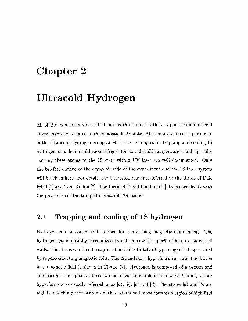
by superconducting magnetic coils. The ground state hyperfine structure of hydrogen
in a magnetic field is shown in Figure 2-1. Hydrogen is composed of a proton and
an electron. The spins of these two particles can couple in four ways, leading to four
hyperfine states usually referred to as la), Ib), Ic) and Id). The states la) and ( b ) are
high field seeking; that is atoms in these states will move towards a,region of high field
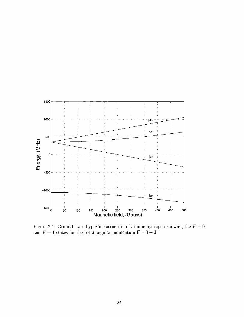
Figure 2-1: Ground state hyperfine structure of atomic hydrogen showing the F = 0 and F = 1 states for the total angular momentum F = I + J
to minimize their potential energy. Hence these atoms are repelled from the magnetic
minimum and are sucked back into the high field region around the discharge (see
Figure 2-2). The Id) and lc) states are low field seeking and both are trapped in a
magnetic minimum which in our experiment presents a trap depth of around 600 mK.
Atoms in the lc) state are lost very rapidly via spin-exchange collisions resulting in a
doubly spin polarized trapped sample of Id) hydrogen atoms. Collisions between two
Id) state atoms occur via a purely triplet molecular potential and spin exchange can
not occur. Atom loss from the doubly polarized sample is dominated by two body
dipole decay [5].
After trap loading, the wall temperature is lowered as quickly as possible (- 20
seconds) from 300mK to around 100 mK. When the wall reaches approximately
150mK, the residence time on the wall for any atom that reaches it becomes so
long that recombination will occur before the atom 'bounces'. At this point there is a
thermal disconnect between the trapped atoms and the cell walls. Any atom escaping
from the trap by evaporation over the magnetic potential will be removed from the
sample.
For the data in this thesis, the trapped cloud was cooled via magnetic field saddle-
point evaporation. The current in the lower pinch magnet is slowly reduced, lowering
th.e axially confining barrier a t the bottom of the trap. The hottest atoms escape,
and after redistribution of the energies of the remaining atoms through collisions,
the sample temperature is reduced. However only atoms with large energies in the
axial direction will be removed. As the atoms settle into the harmonic region at the
bottom of the Ioffe-Pritchard trap, energy exchange between the motional degrees of
freedom decreases and the evaporation becomes largely one dimensional and rather
inefficient [2].
The trapped sample obtained from pushing magnetic field saddlepoint evapora-
tion to its limits has around 10" Id) atoms a t a density of a few 1013 cm-3 with a
temperature of 100 pK and a radial diameter of - 100 pm. The cooling cycle takes
around six minutes. The sample can be further cooled by an radio frequency (rf)
evaporation but this is not done in any of the experiments described in this thesis.
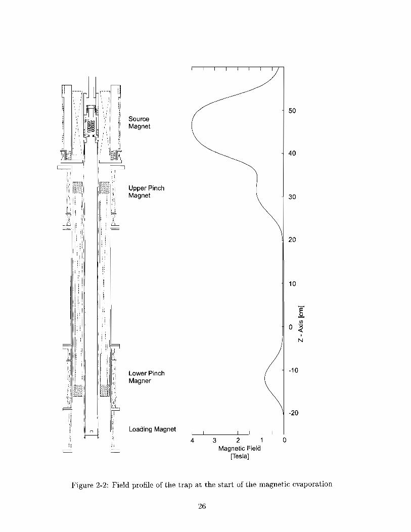
Source Magnet
Upper Pinch Magnet
Lower Pinch Magner
Loading Magnet
4 3 2 1 0 Magnetic Field
[Tes l a]
Figure 2-2: Field profile of the trap at the start of the magnetic evaporation
26

Figure 2-3 shows a schematic of the discharge coil to produce atomic hydrogen, the
cell for confining the atoms and the magnet configuration used for trapping. The cell
is thermally connected to the mixing chamber of an Oxford dilution refrigerator and
the magnets sit in a bath of liquid 4He. Atomic hydrogen is created from molecular
hydrogen by a cryogenic radio frequency (rf) discharge. Molecular hydrogen is frozen
onto the discharge coil during system cooldown. When rf power is applied at the
300 MHz resonant frequency of the coil, molecules are disassociated into atoms and
expelled down into the trapping region. Typically the discharge is run for 8 seconds
at 50 Hz with a 5% duty cycle ( I ms pulses). The peak power of the pulses is around
20 Watts. A single load of 50 T0rr.L of hydrogen lasts for a run of several months.
The trapping cell is a double walled plastic cell with a superfluid helium jacket
between the walls to provide a thermal link between the cell bottom and the mixing
chamber of the dilution fridge. The inside of the cell is covered in a thin layer of
superfluid helium. This film is essential for successful loading. The binding energy of
H atoms on a superfluid 4He film is only 1.1 K, much lower than on any other surface,
arid an atom which is adsorbed onto the cell wall (maintained at 300 mK during
trap loading) during a collision has a good chance of leaving the wall again before it
recombines with another atom to form molecular hydrogen. Any bare spots on the
cell walls during the loading process result in large losses (for a further discussion of
the superfluid film see [6]).
2.2 2s hydrogen production
Once we have prepared a cold, trapped sample of doubly spin polarized ground state
atoms, the next step is to promote some atoms to the first excited (2s) state. This is
a t,wo-photon transition with a natural linewidth of just 0.65 Hz a t 243 nm. To drive
the transition optically, the group developed a continuous wave UV laser source with
a linewidth of atround 2 kHz at 243 nm which can deliver up to 10 mW of light to
the cold atom. cloud. Details of the construction and operation of this laser system
can be found in [4,7]. In a typical experiment in this thesis, we first sweep the UV

bolometer
cell
Figure 2-3: Schematic of cryogenic trapping apparatus taken from [4]. Not shown is an additional small magnet below the lower pinch coil which is used during loading to create a hard end to the trap.

laser across the 1S-2s transition to locate the line center (the frequency which gives
the largest 2s atom number, see the detection method for 2s atoms described in
Section 2.3) and then park the laser a t this center frequency to maximize the 2s
yield.
2.3 2s hydrogen detection
The 2P state in hydrogen is very short lived, decaying in just 1.6 ns. To count the
2S atom number, we apply a small (10 V/cm) quenching electric field across the cell
in order to mix some 2P character into the quantum state of the excited atoms. If
the 2 s sample were left to decay spontaneously, the resulting signal to noise would
be vanishingly small. (The natural lifetime of the 2s state is 120 ms and we have
observed excited atoms to live up to 100 ms in our current trapping cell.) When the
quench field is applied, the excited atoms decay in a few microseconds back to the
ground state by emitting 121 nm Lyman-cu photons. This burst of photons is detected
on a microchannel plate detector (MCP) at the bottom of the experimental cell (see
Figure 2-3). The photon number detected is proportional to the number of 2s atoms
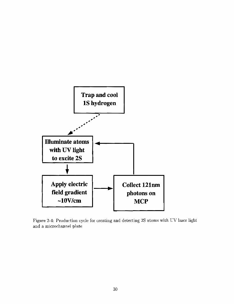
excited. The production and detection cycle is depicted in Figure 2-4. In a typical
load of IS hydrogen, we can perform up to 800 production/detection cycles with the
UV laser on resonance, producing a few tens of millions of excited atoms in each
cycle.
2.4 2s signal - Doppler free and Doppler sensitive
As shown in Figure 2-3, the UV laser beam enters from the top of the cryostat and is
retroreflected with high efficiency from a mirror a t the bottom of the cell. Therefore
the atoms are illuminated with two counter-propagating laser beams of almost equal
intensity. A single atom can absorb two photons from the same beam or a single
photon from each beam. These two cases lead to the dramatically different spectra
illustrated in Figure 2-5. When counter-propagating photons are absorbed, the atom
Trap and cool 1 s hydrogen
I Illuminate atoms 1 with UV light to excite 2 s
Apply electric field gradient
-1OVIcm
Figure 2-4: Production cycle for creating and detecting 2s atoms with UV laser light and a microchannel plate
I I + Collect 121nm
photons on MCP
laser detuning [MHZ at 243 nm]
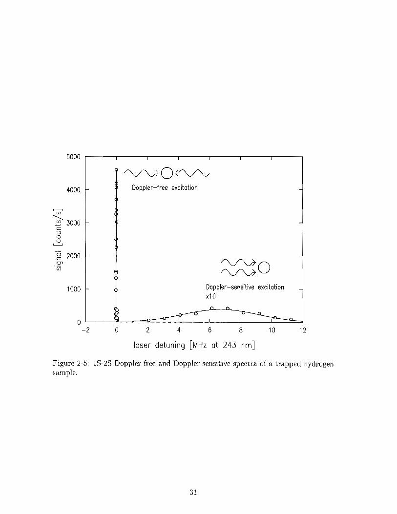
Figure 2-5: IS-2s Doppler free and Doppler sensitive spectra of a trapped hydrogen sample.
receives no net momentum kick, resulting in the intense, narrow line shown on the
left. Because both beams must be in resonance with the atom, this process selects
the cold atoms with no significant velocity in the direction of the laser. Thus the
signal is "Doppler free". The width of this feature is currently limited by our UV
laser system to at few kHz.
If instead an atom absorbs both photons from the same beam, the situation is
markedly different. An atom at rest picks up 2hvk of recoil momentum, causing a
6.7 MHz shift of the center of the line (see Figure 2-5). To supply this extra energy,
the frequency of the photon must be somewhat above half the natural frequency of
the transition. A moving atom can also shift into resonance with a photon that
is detuned from the zero velocity resonance. Hence the Doppler sensitive peak is
strongly broadened due to the finite temperature of the atomic cloud. The Doppler
sensitive spectra was studied extensively in investigations of a hydrogen Bose-Einstein
condensate [8] and can be used in some trap regimes to obtain a measure of the sample
temperature. In the spectroscopic measurements performed in this thesis we use a
laser tuned to the center of the Doppler free line to create a sample of cold, trapped
2s hydrogen.
2.5 2s sample parameters
With a 1 ms UV pulse, we can repeatedly prepare a sample of a few tens of million
metastable 2s atoms in the F = 1, r n ~ = 1 (2s Id)) hyperfine state at densities around
10' cm-3 using the trapped 1s cloud as a reservoir. The 2s cloud is created in the
2 s Id) state because of the selection rules that govern two-photon absorption. These
2s Id) atoms see a potential due to the magnetic field which is essentially identical to
that seen by the IS atoms and hence are also trapped. The metastables are created
in focus of the UV laser beam and then spread throughout the trap by diffusion (see
the discussion in (41). This cold, trapped metastable 2s sample is the starting point
for all the spectroscopic experiments described in this thesis.

Chapter 3
Diode Lasers: properties and
stabilization schemes
Both of the major experiments described in this thesis (see Chapter 6 and Chap-
ters 7& 8) have laser system requirements that are well matched to the properties of
diode lasers. A general discussion of diode lasers and their uses in atomic physics is
given by Wieman and Hollberg in [9]. This chapter summarizes the basics of these
lasers, and describes particular aspects that are relevant to our experiment.
Off-the-shelf, commercially available diode lasers are a very convenient source of
moderately narrow band light (N a few tens of MHz) in the red a'nd infra-red. They
are widely used in telecommunications, optical data storage and consumer electronics
and are therefore cheap, reliable and readily available. This chapter describes some
of the inherent characteristics of diode lasers and covers in detail the external stabi-
lization required to improve the free running linewidth and tuning characteristics to
a point where diodes can be used in a precision spectroscopy experiment.
3.1 Diode structure
Laser diodes are semiconductor devices emitting coherent light. Commercial diodes
come prepackaged in a standard hermetically sealed can with a base flange of either
9 m m or 5.6mm in diameter. A cut-away view of this can is shown in Figure 3-

1 (a). Inside the can is the tiny laser chip with typical dimensions of a few hundred
microns. Because of a high electrical to optical conversion efficiency, these tiny devices
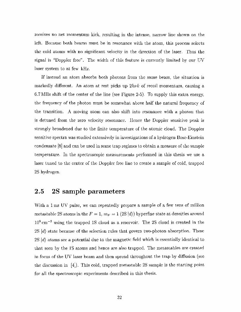
are capable of continuous wave (cw) outputs of tens to hundreds of mW. Figure 3-
1 (b) shows the laser chip structure, the direction of forward injection current and
the characteristic radiation pattern. The optical output is generated by sending an
'injection current' through the active region of the diode between the n-type and p-
type cladding layers. The injection current produces electrons and holes which then
recombine to emit photons. The light is confined within the active region because
of the different refractive indices of the layers. In an index guided laser (the most
common design for moderate power commercial lasers), there is a narrow channel
in the active layer defined by a built-in refractive index profile perpendicular to the
direction of light propagation. This confines the light and defines the spatial mode
of the laser. The rectangular shape of this gain region results in the characteristic
ellipsoidal diode laser beam. The output beam of a diode laser is highly divergent
and must be collimated a short distance from the diode can.
3.2 Tuning characteristics
The band gap of the active layer of a diode is directly responsible for the range of wave-
lengths that can be emitted. The wavelengths of interest in this thesis are covered
by Indium Gallium Aluminum Phosphide (InGaAlP) (the visible range starting at
620 nm) and Aluminum Gallium Arsenide (AlGaAs) (750 to 850 nm). Most commer-
cial lasers can be tuned (choppily and incompletely) over a wavelength range of greater
than 10 nm. This tuning is accomplished by manipulating the junction temperature
and the injection current. For an AlGaAs diode, the frequency of the laser changes
with temperature because both the optical path length of the cavity (+O.O6 nm/K)
and the gain curve (+0.25nm/K) shift with temperature. The wavelength depen-
dence on the injection current is due to both an effect on diode temperature and a
change in the carrier density which changes the index of refraction of the chip and
hence the lasing wavelength. For an AlGaAs laser, the tuning is typically on the
Photodmde Detector
Cladding La ye r (n-l n(CiaA1 )P) Substrate (n-GaAs:) Elect rode
I I
i e k /?=' 1 1
Figure 3-1: (a) The layout of a typical laser diode package. The three leads on the back side of the package are the anode or cathode for the laser diode, the anode or cathode for the internal photodetector (used to run the laser in constant power mode) and a common ground pin. The internal photodiode detector is not used in our experiments and is in fact absent in the 778 nm diodes discussed in Chapter 8. In this case, the third pin in simply not connected. (b) The layers of a typical diode laser chip. Note the highly divergent output beam. Typical values are OI1 = 8" and O1 = 31".

order of -3 GHz/mA for injection currents which are typically in the tens of mA. In-
GaAlP lasers exhibit similar dependencies on temperature and current density. This
rough tunability is very advantageous for initially placing the emission wavelength of
a diode close to that of an atomic transition. However it also then follows that precise
control over the temperature of the diode and the injection current will be of utmost
importance in the inherent stability of any laser diode system.
3.3 Grating feedback stabilization
In a typical laser diode, the uncoated, cleaved facets of the semiconductor chip form
a short, low finesse cavity. The facet reflectivity of - 30% is determined by the index
of refraction of the chip relative to air. Fine tuning of the laser frequency along with a
significant amount of linewidth narrowing is usually carried out via deliberate optical
feedback from an external cavity. The essence of all optical feedback methods is the
same: by increasing the quality factor (Q) of a laser's dominant resonator at some
wavelength, they cause a corresponding decrease in the laser linewidth. According to
[9], no one method has been found that works to narrow the linewidth and control
the frequency of all types of diode lasers. However a method with reasonably wide
applicability for relatively high power (> 15 mW) commercial diodes is that of forming
a pseudo-external cavity laser with frequency selective feedback by using a diffraction
grating.
Grating feedback stabilization works by the formation of an external cavity be-
tween the back facet of the diode and the surface of the grating. Moderate power
commercial diodes tend to have an high reflectance (HR) coated back facet and a
partially anti reflection (AR) coated front facet. This facilitates a design where the
external cavity has a higher Q than the laser chip and hence dominates the internal
diode cavity. With most modern commercial diodes, the window of the protective
can is AR coated and it is not necessary to remove the can to use the laser in a grat-
ing feedback setup. Figure 3-2 shows a roughly to scale sketch of the 'diode block'
which securely holds the diode plus its collimating lens and the grating. It allows

Side view
Slot hinge for vertical
Top view
Diode 0 0 0
grating adjustment
Figure 3-2: Sketch of the block used to securely hold the diode and grating while allowing fine adjustment of the vertical and horizontal pointing of the feedback beam diffracted from the grating.
4-
collim ating l m m m m l m m m m m m l m m m
m m 1 m 1 1 m . 1 m 1 m m m m 1
for horizontal and vertical adjustment of the grating relative to the diode. Vertical
$ rating$p
PZT
0
grating adjustment (changing the angle of the reflected beam in the vertical plane) is
0 0 0 J
provided by a slot hinge in the block itself. A slot hinge in the grating mount provides
horizontal adjustment - manually using a fine thread screw and electronically via a
piezo-electric transducer (PZT) stack [lo]. These diode blocks are based on a design
originally frorn the group of Hansch in Munich, now widely used.
Figure 3-3 illustrates the Littrow configuration that we use in all our grating
stabilized diode lasers. The oth order (reflected) beam is used as the laser output
while the first diffracted order is sent back into the diode1. Tilting the grating changes
the frequency of the light fed back. For practical operation, a tradeoff must be made
between greater feedback and hence greater control over the feedback, versus coupling
'-A di~a~dvantage of this setup is that the pointing of the output beam changes when the grating is rotated.

Figure 3-3: Grating feedback stabilization using the Littrow configuration.
out the maximum possible power. The feedback can be varied by the choice of blaze
angle on the diffraction grating. All the lasers described in this thesis operate in a
grating stabilized configuration with some 10-15% feedback. A laser that must be
pulled far from its free running wavelength will require more feedback than a laser
whose free running wavelength is close to the desired wavelength. We have used a
range of gratings but have now settled on 18001ines/mm gold coated gratings from
Optometrics [ll].
A laser diode in a grating feedback stabilized setup has several major advantages
over a free-running laser diode which more than make up for the loss in optical
power. They are much more likely to lase in a single frequency mode for a wide range
of injection currents and they provide for smooth, reproducible frequency tuning over
hundreds of MHz via a voltage ramp applied to the PZT behind the grating hinge.
In addition, in a well designed setup the linewidth is reduced from the typical free
running tens of MHz to around a few hundred kHz.

, I 1 +-------------- Diode block
Thermoelectric cooler
1 L Sorbothane
Aluminum
Figure 3-4: Sketch of acoustic isolation in laser box design
3.4 Passive frequency stabilization
Our spectroscopy requires that all the lasers lase in a single frequency mode and are
smoothly tunable in frequency over a range of several hundred MHz. As well as the
grating feedback stabilization discussed in Section 3.3, these requirements necessitate
significant attention to the design of the passive components of the system.
Long term single mode behavior with low drift rate requires extremely good ther-
mal and acoustic isolation from the environment. Our laser housings are an 8"x 8"x
5" box made of 0.5" thick aluminum, rigidly mounted to the optical table on 1)' di-
ameter pedestal pillar posts. Inside the box (see Figure 3-4) is a 6" x 6" x 1" block
of copper on a sheet of 0.125" thick Sorbothane. A thermoelectric cooler is sand-
wiched between the diode block and the copper block which acts as both an acoustic
buffer and a heat sink for the diode block temperature control. It is very important
to seal the boxes to eliminate air currents. These boxes ensure that the lasers are
not disturbed by voices or slamming doors. They also deliver good thermal stability.
After the box has been sealed for several hours (the time scale we have observed for
rea,ching thermal equilibrium), the frequency drift (part of a random wander) is only
around 1 MHz in. a minute.
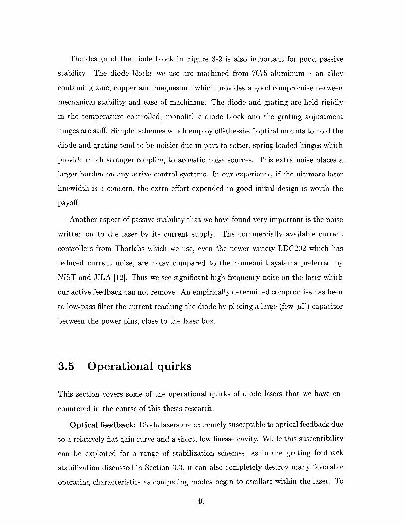
The design of the diode block in Figure 3-2 is also important for good passive
stability. The diode blocks we use are machined from 7075 aluminum - an alloy
containing zinc, copper and magnesium which provides a good compromise between
mechanical stability and ease of machining. The diode and grating are held rigidly
in the temperature controlled, monolithic diode block and the grating adjustment
hinges are stiff. Simpler schemes which employ off-the-shelf optical mounts to hold the
diode and grating tend to be noisier due in part to softer, spring loaded hinges which
provide much stronger coupling to acoustic noise sources. This extra noise places a
larger burden on any active control systems. In our experience, if the ultimate laser
linewidth is a concern, the extra effort expended in good initial design is worth the
payoff.
Another aspect of passive stability that we have found very important is the noise
written on to the laser by its current supply, The commercially available current
controllers from Thorlabs which we use, even the newer variety LDC202 which has
reduced current noise, are noisy compared to the homebuilt systems preferred by
NIST and JILA [12]. Thus we see significant high frequency noise on the laser which
our active feedback can not remove. An empirically determined compromise has been
to low-pass filter the current reaching the diode by placing a large (few PF) capacitor
between the power pins, close to the laser box.
3.5 Operational quirks
This section covers some of the operational quirks of diode lasers that we have en-
countered in the course of this thesis research.
Optical feedback: Diode lasers are extremely susceptible to optical feedback due
to a relatively flat gain curve and a short, low finesse cavity. While this susceptibility
can be exploited for a range of stabilization schemes, as in the grating feedback
stabilization discussed in Section 3.3, it can also completely destroy many favorable
operating characteristics as competing modes begin to oscillate within the laser. To

guard against such accidental feedback, we use an optical Faraday isolator2 with 40-
60dB of isolation directly in front of each laser, just outside of the aluminum box.
The isolator must be carefully aligned and adjusted for the appropriate wavelength.
Elven with the isolator in the beam line, direct reflections must be avoided. We have
on occasion seen optical feedback coming from a surface which is separated from
the isolated laser by an optical fiber. Another tradeoff must be made here between
output power and susceptibility to optical feedback. Lasers with strong, deliberate
optical feedback used to control the frequency will be correspondingly less sensitive
to accidental feedback from stray beams, but will have less power in the primary
(output) bea,m.
Transients: Diode lasers can easily be destroyed by brief electrical transients
which cause too much current to flow or produce too large a back voltage across the
junction. These transients can often occur in power up or power down. Current
controllers built to be used with diode lasers should be equipped with a soft on/off
function. Extreme care is also needed when handling the bare diodes as the static
electricity built up on a user on a dry Boston day is more than enough to destroy a
diode.
Collimation: As mentioned in Section 3.1, the output beam from a diode laser is
strongly divergent. Hence the beam needs to be collimated a short distance from the
diode with a small f number lens. We have had good success with the Geltech range
of lenses from Thorlabs, particularly the C230TM-B. The quality of the collimation
is very important in achieving good results within a grating feedback setup - the lens
position needs to be adjusted to give a spot of a fixed diameter over several meters.
3.6 Diode lasers for 2s-3P spectroscopy
This section discusses the issues involved in selecting a diode for spectroscopy a t
656nm, the wavelength of the 2s-3P transition in hydrogen (see Chapter 6). The
features of interest are:
2 ~ e have used two brands of isolators, Optics for Research and Linos Photonics.
41

available power (at least 15 mW after stabilization)
single mode behavior
smooth tunability
compatibility with a grating feedback setup.
Reliable diode lasers at 656 nm are not readily available, possibly because of the
large gap between 656nm and the telecom wavelengths in the IR that tend to drive
commercial development. In the course of the experiments reported in this thesis,
we have only found one acceptable option - the Panasonic LNCQ05PS 5.6mm. Un-
fortunately, this diode is no longer manufactured. Happily, new diodes are regularly
being developed so a recommendation for future experiments would be to try out any
diodes which have gone into production since 2003.
Available power: Spectroscopy of the one-photon 2s-3P transition requires only a
few pW of light (see Section 6.5.4). The power requirements for the laser diode are
instead set by the amount required to perform saturated absorption in iodine (see
Chapter 4). Some 20 mW is a comfortable amount of power at 656 nm. The power vs
injection current spectrum for a grating stabilized Panasonic is shown in Figure 3-5.
Note that this spectrum shows power before the optical isolator which will reduce the
total available power by N 10%) depending on alignment.
Single mode behavior: To be a useful spectroscopic tool, the laser needs to lase in
a single longitudinal mode when operating in a grating feedback stabilized configu-
ration3. Finding a laser that lases in a single longitudinal mode while sweeping over
hundreds of MHz was the single biggest problem encountered in our search for 656 nm
diodes. Single mode and multi mode output from a typical Panasonic LNCQ05PS
are shown in Figure 3-6.
Smooth tunability: The range of continuous tunability for different brands of
diodes is surprising. The range of smooth tunability is the range in frequency over
30ne point worth noting is that some diodes are advertised as 'single transverse mode' meaning the output beam has only one spatial mode. In our experience, all the lasers we have tested have had a single spatial mode.

0 I I I I I I I I
20 30 40 50 60 70 80 90 100 110 120
Current, (mA)
Figure 3-5: Output power directly from the grating stabilized laser vs injection cur- rent. The threshold current for lasing is several mA lower than in the free running laser. Reduction in the threshold current is an indication of grating stabilization via optical feedback. The reduction depends on the alignment of the grating and the percentage feedback. The maximum current plotted above is determined by the manufacturer's absolute maximum rating and varies from diode to diode.

-500 -400 -300 -200 -100 0 100 200 300 400 500
Detuning, (MHz)
Figure 3-6: Single mode (top) and multi mode (bottom) behavior for a typical Pana- sonic LNCQ05PS operating in a grating stabilized configuration. The frequency scale
0.8 0, .-
0.6
u 2 0.4 (d 0
along the x axis is approximate and is taken from a relative measurement of the voltage span needed to reach the full spectral range (FSR) of the Fabry Perot cavity used as a frequency discriminator. The apparent width of each individual mode is dominated by the width of the modes of the cavity. Because the cavity is confocal,
0 0.2 -
0 -700 -600 -500 -400 -300 -200 -100 0 100 200 300
Detuning, (MHz)
- -
it is mode-degenerate i.e. zeroth and higher order modes all almost overlap. The ap- parent width of the cavity therefore depends on the precise alignment but is usually around the 10 MHz seen here.
-
-
-
-
I

which a diode can be swept by varying the voltage of the PZT behind the grating
hinge while maintaining single mode behavior and avoiding mode hops4. Within a
given brand, behavior from diode to diode varies little. Most of the 656nm diodes
scanned smoothly over acceptable ranges.
Compatibility with a grating feedback setup: Grating feedback stabilization
works significantly better (in terms of tunability achieved and feedback power re-
quired) in some brands of lasers than in others. The reasons for this are not clear
but probably depend on the actual fabrication methods employed for various diodes.
The Panasonic was the only diode investigated that combined reasonable mode be-
havior with the required output power and tunability when operated with grating
stabilization.
Diode lasers for 2s-8s spectroscopy
The 2s-8s transition is a two-photon transition at 778nm. Spectroscopy of this
transition is discussed in Chapters 7 and 8. Although several manufacturers sell
diodes in this wavelength range, we have had reasonable results with only a few
diodes.
Available power: With the 778 nm laser system, available optical power is of much
greater concern than for the system a t 656nm. The iodine saturated absorption re-
quires more power (see Section 8.2) and, as described in Chapter 8, the two-photon
2s-8s hydrogen spectroscopy is estimated to require more than 50 mW of light rather
than the p W that are sufficient at 656nm. Monitoring of the laser frequency and
mode quality, which is essential in our precision measurement experiments, also re-
quires significant power. The total power required is more than can be provided by
a single laser running under grating feedback (see Chapter 8). An injection locked
diode laser system was built to overcome this limitation and provide sufficient power. -
4There are many clever schemes to obtain GHz scans which involve scanning the PZT voltage in tandem with a simultaneous injection current sweep. However, as sweeping a few hundred MHz is all that is regularly required in our experiment, we wished to avoid the additional complexities of these implement- CL t ' ions.

This system is discussed in Section 8.3. Although our current powers are marginal,
available powers seem to be increasing almost every year.
Single mode behavior: By and large, diodes close to 778 nm seem to run single
mode at almost all injection currents even without grating feedback stabilization.
Smooth tunability: Several brands of diode were tried that would not give wide
( N GHz) scanning ranges although they would lase single mode at almost any given
injection current. However the Hitachi HL7851G, the Sanyo DL7140-201s and the
Sharp GH0781JA2C all perform well. These are all fairly recently available diodes,
so the poor scanning may have been due to a structural problem that was resolved
in newer products.
Compatibility with a grating feedback setup: For grating feedback opera-
tion we have had success with the 50 mW Hitachi HL7851G and the 120 mW Sharp
GH0781JA2C. Strangely the 80 mW Sanyo DL7140-201s does not work well.
Injection locking: As slave lasers for injection locking (see Section 8.3), the 50 mW
Hitachi HL7851G, the 80 mW Sanyo DL7140-201s and the 120 mW Sharp GH0781 JA2C
all work well.

Chapter 4
Iodine Frequency Reference
In the search for any atomic signal, a pre-requisite is absolute frequency calibration -
the ability to place the spectroscopy laser as near as possible to the frequency of the
desired transition. In this chapter, we explain the procedure for observing an iodine
spectrum using saturated absorption spectroscopy, and then stabilizing or 'locking' a
diode laser to the desired spectral line. The spectrum of molecular iodine is frequently
used in laser spectroscopy as a frequency reference. For example, iodine is the basis
of frequency references a t 532 nm (second harmonic of a Nd:YAG laser) and 632 nm
(iodine-stabilized He:Ne lasers). The rotational and vibrational level structure of the
excited I2 m01.ecule provide a rich structure of lines, the strongest of which have been
documented experimentally across the upper visible and lower infra-red spectrum
(500nm-909nm) by Gerstenkorn and colleagues [13]. More recently, a program for
calculating the spectrum at a given wavelength was developed at the Institute of
Quantum Optlics, University of Hannover. It is now commercially available under
the brand name of IodineSpec4 from Toptica Photonics AG. This chapter covers the
design and construction of a molecular iodine frequency reference for use in the 2S-3P
and. 2S-8s experiments described in Chapters 6, 7 and 8.

Dual
Iodine oven
Figure 4-1: Saturated absorption setup for iodine spectroscopy. PBS stands for po- larizing beam splitter.
4.1 Saturated absorption spectroscopy of molecu-
lar iodine
In simple absorption spectroscopy, the observed linewidths in molecular iodine at
room temperature are around 900 MHz. These broad lines actually consist of a num-
ber of hyperfine components, smeared out and overlapped by Doppler broadening of
- 300 MHz. In order to observe the underlying N 10 MHz hyperfine iodine signals,
one can suppress the broad Doppler profile using a technique known as Doppler-free
saturated absorption spectroscopy (DFSAS) [14]. The optical setup for this spec-
troscopy is shown in Figure 4-1. For a DFSAS setup, a single beam is split into
three - two relatively weak probe beams and a stronger pump beam. The probe
beams both travel in the same direction through the gas cell and are directed onto
photodiodes which measure the intensity as a function of time. The pump beam is
positioned to overlap with one of the probe beams1. The non-overlapped probe beam
gives the standard Doppler broadened absorption signal. However the second probe
beam travels the same path through the iodine cell as the counter-propagating pump
beam. The pump beam causes a partial population inversion in the iodine atoms
it interacts with. This results in dips in the Doppler broadened absorption seen by
the probe, whenever the pump and probe are in resonance with the same group of
'To boost the iodine signal in the infrared, the pump and probe beams are overlapped for the full length of the iodine cell. This requires the use of polarization optics to protect the diode from optical feedback due to the retroreflected pump beam.
atoms i.e. at the zero velocity frequency of each spectral component. Subtracting the
two probe beam absorption signals removes the common mode Doppler broadening,
leaving only the 'dips'.
4.2 Experimental considerations
4.2.1 Lock-in detection
The simple implementation of DFSAS described in Section 4.1 works well for absorp-
tion signals which are reasonably strong. In the case of iodine however, even with a
heated cell, t,he lower states of the transitions of interest are only weakly populated
and we need to use lock-in detection to lift the correspondingly tiny absorption signals
out of the noise. (For details of lock-in detection, which is a standard technique, the
interested reader is referred to [15]). However, there is one experimental quirk which
requires explanation. In lock-in detection an externally imposed, periodic excitation
serves to dissociate the output signals from random disturbances. In our experi-
ments, the periodic excitation is a 'fast' sinusoidal modulation of the laser frequency.
The laser is 'slowly' swept in frequency across the spectral region of interest and the
differential ou.tput absorption signal from the two probe beam photodiodes2 is demod-
ulated by a EG&G Model 5204 Lock-In Analyzer using a reference signal from the
same function generator that is used to impose the 'fast' sinusoidal modulation. The
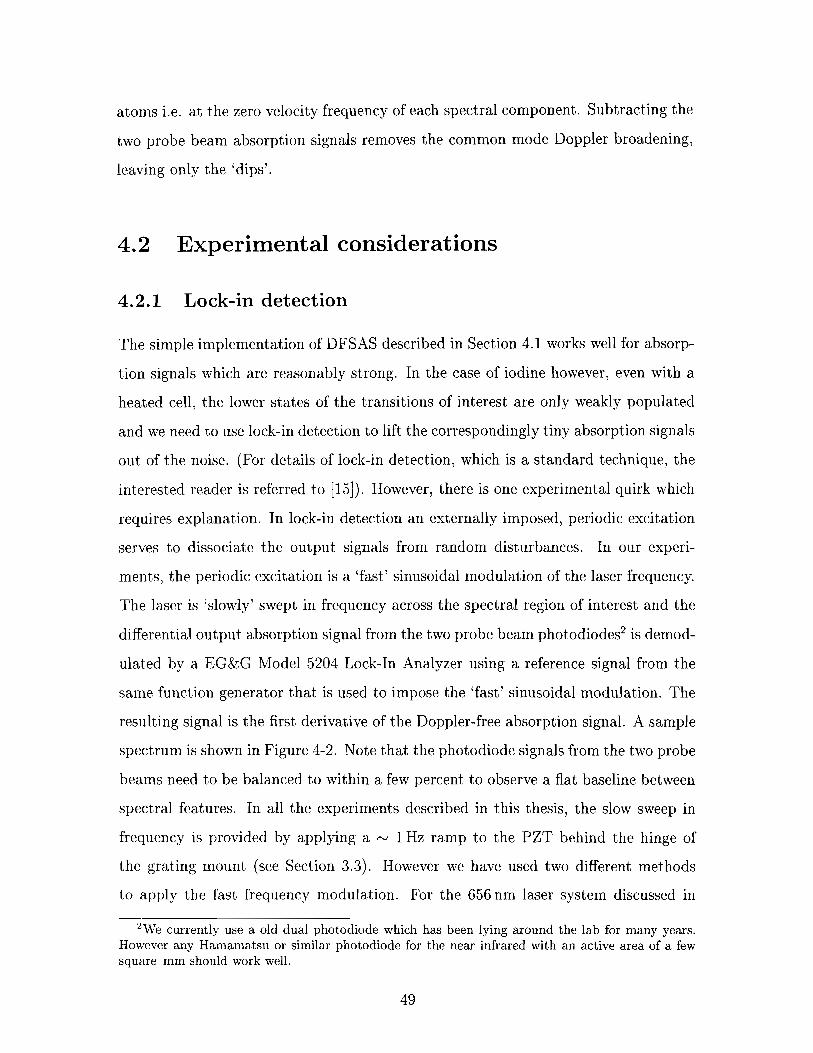
resulting signal is the first derivative of the Doppler-free absorption signal. A sample
spectrum is shown in Figure 4-2. Note that the photodiode signals from the two probe
beams need to be balanced to within a few percent to observe a flat baseline between
spectral features. In all the experiments described in this thesis, the slow sweep in
frequency is provided by applying a 1 Hz ramp to the PZT behind the hinge of
the grating mount (see Section 3.3). However we have used two different methods
to apply the fast frequency modulation. For the 656nm laser system discussed in -
2We currently use a old dual photodiode which has been lying around the lab for many years. However any Hamamatsu or similar photodiode for the near infrared with an active area of a few square mm should work well.

I
Wavenumber (cm-l) (full scale -0.03 cm-') I
Figure 4-2: Experimental iodine spectrum in the 656 nm region. The extent of the x axis in wavenumber is estimated to be 0.03 cm-I from comparison with the theoretical spectrum. dA/dn is the change in absorption with wavenumber. The absolute voltage scale for the y axis depends on laser power, alignment, modulation depth, lock-in settings, etc.

Chapter 6, the fast modulation is applied using current modulation applied through
the laser current controller. The major drawback is that the frequency modulation of
the iodine laser limits the achievable linewidth. For performing spectroscopy on the
30 MHz wide 3P state however this is not a significant issue.
The second approach we used for the fast modulation is to use an acousto-optic
modulator (AOM) to modulate the pump beam. The modulation amplitude is typi-
cally 8 MHz and the modulation rate around 50 kHz. The AOM technique results in
a much cleaner absorption signal with a flatter baseline between absorption peaks.
This is important for reliably locking the laser at 778nm where the iodine absorp-
tion is lower and the signals correspondingly lower. The downside is a significantly
greater expense (AOM plus driver costs on the order of several thousand dollars) and
a severe loss in available light power. In order to avoid problems with pump beam
motion as the driving radio frequency (rf) is modulated, the light must be double
passed through the AOM giving at most -- 50% of the input light in a usable output
pump beam3. Because the modulation is externally applied only to the pump beam,
there is no frequency modulation of the laser itself. This allowed us to keep the line
width of the iodine laser narrow. This is important in the phase locking experiments
described in Section 8.5.
4.2.2 Optimizing the absorption signal
The molecular iodine spectrum is unlike an atomic absorption spectrum which usually
consists of a few well separated lines. In iodine, there are many possible lock points of
comparable height and slope within a small frequency range. A good signal-to-noise
ratlio and a flat baseline are both important in obtaining a stable laser frequency
lock to a given line that will reliably stay at , and re-lock to, the same point. The - -
3Note that it is certainly possible to achieve much higher double passed efficiency with an AOM but this requires using a beam which is collimated as it passes through the crystal. A collimated beam must be reflected off a flat mirror, but a flat mirror can be normally orientated to the beam for only one AOM frequency and a setup like this will still result in a significant change in pointing of the double passed beam as the rf frequency is swept. In order to observe a clean FM signal (without additional AM from pointing modulation), the AOM must be a t the focal point of a confocal telescope. This introduces significant divergence into the beam as it passes through the crystal and reduces the achievable diffraction efficiency into the first order.

experimental absorption signal as described in the previous sections is relatively easy
to observe, but it can be challenging to optimize. The optical setup used is shown in
Figure 4-1. Reflections back into the diode laser must be carefully avoided by placing
the oven and the photodiodes at slight angles to the incoming light beams. The
photodiodes monitoring the two probe beams are very susceptible to scattered light,
while the lock-in signal is easily distorted by an imbalance in the two probe beam
intensities. We have found the alignment of the iodine optics critical to obtaining a
reliable lock signal. In the 656 nm setup (which is less demanding in terms of power
requirements) it is worth sacrificing light power to decouple the iodine alignment from
the laser alignment by an optical fiber. With this setup, on a day-to-day basis the
only alignment that is usually necessary (even when the grating must be realigned to
tune the laser frequency) is to peak up the fiber coupling. This becomes especially
important for an inexperienced operator. Unfortunately, with currently available
diodes, the power loss due to the optical fiber is too great to be supported in the
778 nm system where iodine spectroscopy requires all the power we have available.
4.3 Locking to iodine
In all the experiments described in Chapters 6, and 8, we use a two-laser setup where
one laser provides a frequency reference via iodine spectroscopy and the other can
be swept in frequency relative to the reference laser to perform the spectroscopy.
This section discusses the techniques involved in locking a diode laser to an iodine
transition to provide the frequency reference.
The first step in locking the reference laser to iodine is observation of the DFSAS
signal at the desired frequency. There are many extremely similar absorption spectra
- the exact spectrum of interest becomes familiar with time. For the 2s-3P transition,
we use a old Burleigh WA-10 wavemeter to initially tune the laser close to the required
15233.36 cm-'. Careful attention to the reading of the wavemeter is necessary as there
is a largely indistinguishable spectrum only 0.2 cm-' away. After initial alignment of
the grating to reach the correct frequency, day-to-day adjustment should be possible

by changing only the diode injection current and the PZT voltage. To unambiguously
identify the iodine spectrum of interest, it is necessary to sweep over a range of several
hundred MHz (see Figure 4-3 a)) . To do this, the PZT behind the grating hinge is fed
the sum of the slow ramp and a variable DC offset. Any small area of the spectrum
within the sweep can be selected by adjusting the amplitude of the ramp and the value
of the offset. In this way, the desired lock point is brought to the center of the sweep
(see Figure 4:-3 b)). When just one zero crossing remains within the sweep range, the
- - - -
Wavenumber (em-') (full scale -0.03cm-')
Wavenumber (cm-') (full scale -0.002cm-')
Figure 4-3: a) Sweep across all the features in the iodine band closest to the H 2S-3P transition frequency. PZT voltage sweep is around 8 V. b) Zoomed sweep across one fea,ture. PZT voltage sweep is around 600 mV.
electronic lock is switched on, holding the laser frequency a t the point corresponding
to that zero. At present this feedback system is a simple low bandwidth PI controller
(see Figure 4-4) which feeds back only to the grating PZT. This setup holds the laser
in lock for many hours. The observed linewidth is on the order of 2 MHz. As long as
the laser stays locked to the same iodine feature, the center frequency is not observed

Figure 4-4: Loop filter for grating lock to iodine. The first two op amps buffer the input signal and add a variable DC offset. The third buffers an output for use as a monitor. All the resistors represented by zigzagged lines are the same, non-critical value. The last two op amps provide the loop filter shaping.

to drift on the MHz scale which is sufficient for our purposes.
4.4 Iodine oven
For all of the frequencies of interest in our experiments, the lower level of the iodine
transition in question is only weakly populated at room temperature. Hence to obtain
reasonable signals, the iodine cell must be heated. In early experiments at visible
frequencies, we used a 10 cm long cell at around 40°C. This provided an adequate
signal for light at 656 nm but not for transitions in the infrared which start from a
higher vibrational state. To observe these signals we needed a setup that could be
maintained aJt higher temperatures and provide a longer optical path length in the
gas.
To address the second issue, we purchased a custom iodine cell from Opthos
Instruments [16]. It is 25 mm in outer diameter and 300mm long with a 60 mm
tipped off filling stem close to one end. The material is quartz with optical quality
windows optically contacted to the cell body. The cell is held inside the oven without
touching the sides to avoid spot heating. A thermocouple [17] is attached to the side
of the cell to measure the oven temperature.
A new oven was also designed and built to produce the - 600" C temperatures
required (see Figure 4-5). The heart of the oven is a 40 mm diameter stainless steel
tube. It is 250 mm long with a slot cut in one end to accommodate the tipped off filling
stem of the iodine cell which is used as a cold finger. Wrapped around the outside of
the central 10 cm of the tube is a quartz insulated heating cord rated to 800°C [18].
The stainless steel tube with attached heater wire was wrapped in a ceramic fiber
insulation blanket [19] to make a bundle with outer diameter - 120 mm. This was
pla'ced inside a 50mm thick tube of mineral wool pipe insulation [20]. Corrugated
aluminum pipe insulation [21] was wrapped around the mineral wool tube to form
the outer layer of the oven. End pieces were cut from the same aluminum insulation.
This oven has now been continuously operated at 600°C for many months.
In order to observe the - 10MHz absorption lines, it is necessary to control the

Aluminum cladding McMaster Carr #4479K15
Mineral wool tube insulation McMaster Carr #9364K59
Stainless steel tube wrapped in quartz insulated heating tape
Ceramic fiber insulation blanket McMaster Carr #93315K61
Figure 4-5: Schematic of iodine oven showing construction materials. Material choices are limited at the required 600' C.
a,mount of iodine in the cell. This avoids the collisional broadening which otherwise
washes out the features. The iodine cell cold finger extends some 2" from the body
of the cell. For the experiments in this thesis, we kept its tip immersed in water to
hold it close to room temperature hence limiting the pressure of iodine in the cell.

Chapter 5
Detection of the 2s-4P transition
In 2001, the group purchased a second tunable dye laser system to construct a narrow
band UV light source for precision 1s-2s measurements. We took advantage of our
new capabilities to gain experience in detecting transitions from the 2s state by
observing the 2s depletion while pumping the 2s-4P transition.
It is difficult to introduce new techniques for ultracold hydrogen because of the
complexity of the apparatus. There is a long turn around time for any apparatus
alterations and alterations to the trapping cell carry a grave risk of opening up leaks
which can only be detected a t helium temperatures. With a dye laser, we had unlim-
ited optical power and could essentially fill the cell with 2s-4P light, eliminating the
complications associated with beam-atom cloud alignment and removing the need to
have a high reflectance mirror for 486 nm light at the bottom of the cell (see Chap-
ter 6).
In the hydrogen atom, the level structure is such that
or in other words, v(2S - 4P) falls only 4.87 GHz from the frequency of the blue
light (486nm) that , when doubled (to 243nm), is used to pump the two-photon,
ultraviolet 1 S-2s transition (1 2 1 nm) . Other researchers have used this coincidence of
frequencies to make precision Lamb shift measurements by comparing the 1s-2s and

2s-4P frequencies [22].
5.1 2s-4P laser
The laser used in these measurements is an off-the-shelf Coherent 899 ring dye laser
circulating Coumarin 480 dye and pumped with a Coherent Sabre Krypton ion laser.
The linewidth of the laser locked to its internal reference cavity is approximately
1 MHz which is significantly less than the 12 MHz natural line width of the 2s-4P
transition.
The lasing frequency is grossly adjusted by adjusting the intracavity etalon and
the birefringent filter. The frequency can be smoothly scanned over a range of several
GHz by scanning the internal Fabry-Perot reference cavity to which the laser is locked.
5.2 Frequency reference
Because of the close coincidence of transition frequencies, the experiment ally deter-
mined a u ( l ~ - 2 s ) frequency can be used as a frequency reference to locate the
v(2S - 4P) frequency. A small portion of 486 nm light from the 1s-2s laser system
was split off and sent to the second dye laser in a single mode fiber. We then tuned
the second dye laser until the readings of both lasers were the same on our Burleigh
WA-10 wavemeter to within 0.01 cm-' or 0.3 GHz '. The light from the two lasers
was superimposed on a fast photodiode [23]. The resulting beat signal was mixed
down with a - 5 GHz local oscillator to a few hundred MHz which can be observed
on a standard 1 GHz range spectrum analyzer (in this case a Hamamatsu HM5011).
The laser frequency was scannable via computer by running a control signal to the
analog input on the Coherent control box.
'While the Burleigh cannot be relied on for absolute accuracy, if two lasers simultaneously give the same reading, they will be within a few hundred MHz of each other.

Trap and cool 1S hydrogen
2s cloud
Excite 2S-4P transition metastables
Figure 5-1: Experimental cycle at each blue frequency point for the 2S-4P depletion experiments
5.3 2S-4P results
We were essentially unlimited in the input blue power - the saturation intensity of
the 2S-4P transition is around a p W (see Chapter 6) and dumping ten times this
power into the cryostat for a few ms does not cause significant heating. Because
the retroreflecting mirror at the bottom of the cell had only around a 10% reflection
for 486 nm light, we did not attempt to use a blue beam waist at the cloud and
obtain a retroreflected beam. Instead, we used a roughly collimated beam a few mm
in diameter, filling the cell with 2S-4P light and removing the stringent alignment
constraints that must be considered in Chapters 6 and 7.
Figure 5-1 shows a flowchart of the experimental cycle used to observe the 2S-
4P transition. The signature is a depletion in the number of metastable 2s atoms
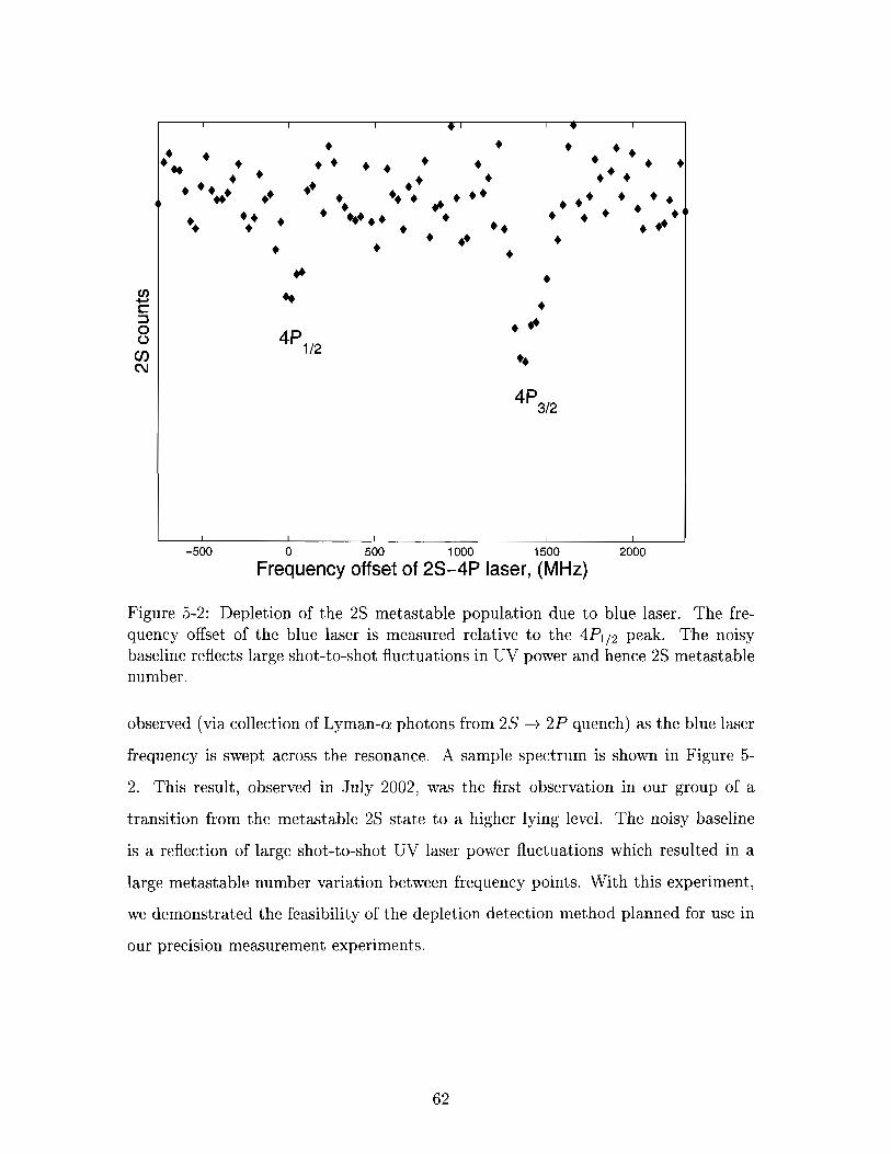
-500 0 500 1 000 1500 2000
Frequency offset of 2s-4P laser, (MHz)
Figure 5-2: Depletion of the 2s metastable population due to blue laser. The fre- quency offset of the blue laser is measured relative to the 4Pl12 peak. The noisy baseline reflects large shot-to-shot fluctuations in UV power and hence 2s metastable number.
observed (via collection of Lyman-a photons from 2 s + 2 P quench) as the blue laser
frequency is swept across the resonance. A sample spectrum is shown in Figure 5-
2. This result, observed in July 2002, was the first observation in our group of a
transition from the metastable 2s state to a higher lying level. The noisy baseline
is a reflection of large shot-to-shot UV laser power fluctuations which resulted in a
large metastable number variation between frequency points. With this experiment,
we demonstrated the feasibility of the depletion detection method planned for use in
our precision measurement experiments.

Chapter 6
Spectroscopy of the 2s-3P
transit ion
6.1 Motivation
This chapter describes the lab's first steps in the area of Balmer-n spectroscopy of
trapped atomic hydrogen. There are two reasons for performing this spectroscopy.
The first is that the required 2s-3P laser system is extremely similar to the more
complex 2s-8s system discussed in Chapter 8. The iodine locking electronics, beat-
note detection, and computer interface with the experiment are identical. The optical
setup is similar and for the spectroscopy itself the alignment issues are less stringent
(a one-photon transition doesn't require overlapping counter-propagating beams a t
the atomic cloud). These similarities allowed us to use experiments with the 2s-3P
laser system as a testing ground for the proposed 2s-8s experiments. The 2s-3P
traasition has a natural width of 29 MHz compared to the 2s-8s width of 72 kHz at
778 nm and, because the transition is via a single photon, the expected depletion sig-
nal is an order of magnitude larger for only a tiny fraction of the light power. These
experiments are described in Section 6.4.
The second reason is to investigate the feasibility of using absorption spectroscopy
on the 2s-3P transition as a detection method for 2s atoms. The current method,
in which Lyman-n photons are detected on a cryogenic microchannel plate, suffers

from the extremely restricted cell geometry imposed by the magnet configuration
and poor detection efficiency. Section 6.5 describes our preliminary observations of
Balmer-c-u absorption spectroscopy. Section 6.6 estimates the signal to noise that can
be expected from the two detection methods.
6.2 Laser layout for spectroscopy
In order to perform spectroscopy of an atomic transition we have the following re-
quirements:
a frequency reference to place us within a few linewidths of the atomic frequency
sufficient power to drive the transition
the ability to sweep the frequency across the transition
The laser setup in Figure 6-1 was designed to meet all these requirements using a
pair of grating stabilized diode lasers. As discussed in Section 6.3 and in detail in
Chapter 4, the frequency reference for our 2s-3P experiments is provided by saturated
absorption spectroscopy of molecular iodine. For this one-photon transition, the
power required to drive the 2s-3P transition is a few hundred nW (see Section 6.5.4).
This is only a tiny fraction of the power available from a single diode. Of greater
importance from a system design standpoint is the requirement that we can sweep the
laser frequency across a frequency range of several times the 30 MHz linewidth. With
a single laser setup, this frequency sweep capability would have to be provided by an
acousto-optic modulator (AOM) limiting the total sweep range to less than 100 MHz.
In addition, an AOM has a steep fall off in diffraction efficiency as the drive frequency
moves away from its designed center frequency. Hence for even a small sweep range,
there would be significant variation in diffracted power compounded by a variation
of the coupling efficiency into the fiber used to transport light to the atoms. This
power variation with varying frequency would make the obtained spectra difficult to
interpret.

Iodine saturated absorption
Fiber coupler to wavemeter
n Fiber coupler 4- ,La--
S u cu alum; Fiber coupler to wavemeter I
Optical beatnote free space coupled to 1, New Focus 1577 PD \ I
Iodine reference laser
I
Spectroscopy laser
Figure 6-1: Laser pair layout for atomic spectroscopy a t 656 nm. FP cavity refers to the Fabry-Perot spectrum analyzer used for monitoring the laser mode. The waveme- ter used was a Burleigh WA-10. The New Focus photodiode has a bandwidth of 12 GHz, rather more than is required for this experiment.

To avoid these problems, a paired laser system was constructed as shown in Fig-
ure 6-1. One laser is locked to a line in molecular iodine. Some light from each laser
is then overlapped on a fast photodiode to form an optical beatnote. An offset lock is
formed whereby the second diode is locked to the first diode with the frequency off-
set determined by a computer-controlled radio frequency synthesizer. (For details of
offset locking two diode lasers see Chapter 8.) By varying the synthesizer frequency,
we can sweep the frequency of the spectroscopy laser relative to the iodine laser while
maintaining the lock.
6.3 Saturated absorption of iodine at 656 nm
Molecular iodine provides an excellent frequency standard for our 2s-3P experiments,
placing us within a few tens of MHz of the desired transition. The details of saturated
absorption spectroscopy in iodine are discussed in Chapter 4. With the oven at 200' C
(the iodine tip is immersed in water to hold it at room temperature), the Doppler
broadened, single pass absorption around 15233.36 cm-'(656 nm) is on the order of
30%.
Figure 6-2 shows the first derivative of the Doppler free absorption signal obtained
around 656 nm. In the iodine atlas [13], the centroids of the rotational fine structure
around the 2s-3P transition frequency have been analyzed experimentally to an un-
certainty of around 30MHz. Allowing for effects due to temperature, pressure and
possible impurities in the iodine cell, we expected an absolute accuracy of around
50 MHz which is indeed comparable to what we observed. As we were searching for a
30 MHz line and had a sweep range approaching a GHz, this accuracy was perfectly
accept able.

Relative amplitude of lock-in signal, (dA/dn)
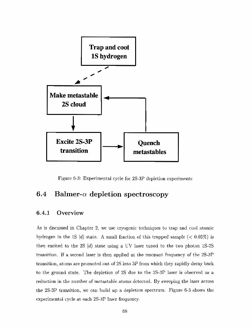
Trap and cool 1s hydrogen
Make metastable I 2s cloud
Excite 2s-3P transition metastables
Figure 6-3: Experimental cycle for 2s-3P depletion experiments
6.4 Balmer-a depletion spectroscopy
6.4.1 Overview
As is discussed in Chapter 2, we use cryogenic techniques to trap and cool atomic
hydrogen in the 1s Id) state. A small fraction of this trapped sample (< 0.05%) is
then excited to the 2s Id) state using a UV laser tuned to the two photon 1s-2s
transition. If a second laser is then applied at the resonant frequency of the 2s-3P
transition, atoms are promoted out of 2s into 3P from which they rapidly decay back
to the ground state. The depletion of 2s due to the 2s-3P laser is observed as a
reduction in the number of metastable atoms detected. By sweeping the laser across
the 2s-3P transition, we can build up a depletion spectrum. Figure 6-3 shows the
experimental cycle at each 2s-3P laser frequency.

6.4.2 Beam alignment
In contlrast with the 2s-4P experiments described in Chapter 5, for the 2s-3P light
we could expect to see a reflected beam off the mirror on the bottom of the cell (HR
@ 243 nm and 656 nm). The return beam is extremely useful for initially aligning the
red beam with the cloud. If the red light overlaps with the UV beam on the fridge
top window and we have a return beam which overlaps the in-going red beam, the
path of the UV and red beams in the fridge will be similar. A return spot close to
the fiber tip, maximized in brightness by eye, would usually give sufficiently good
alignment to observe some depletion.
6.4.3 2s-3P depletion results
A typical spectrum is shown in Figure 6-4. It is obtained by scanning the red laser
frequency across the 2s-3P transition while holding the UV laser fixed to maximize
2S atom number production. The plotted data is the averaged sum of 20 sweeps
across the 2s-3P line. About 450 nW of power was used in a 1 ms pulse. The beam
waist at the cloud was around 100 pm.
In this depletion experiment, we are considering the case where the atoms interact
with a light field of roughly constant intensity throughout the length of the cloud (i.e.
the percentage nbsorption of the light is small). If the excitation rate at frequency
w is y(w), then the number of atoms after excitation time t is N = ~ ~ e - ' ( ~ ) ~ and
the number of decay photons observed on the MCP after quenching the metastable
atoms is C = ~ ~ ~ e - 7 ( ~ ) ~ where c is the overall detection efficiency include the factor
from the restricted cell geometry. From the observed signal C , we want to extract
y(w). For a fixed pulse duration T
= - 1nC + const
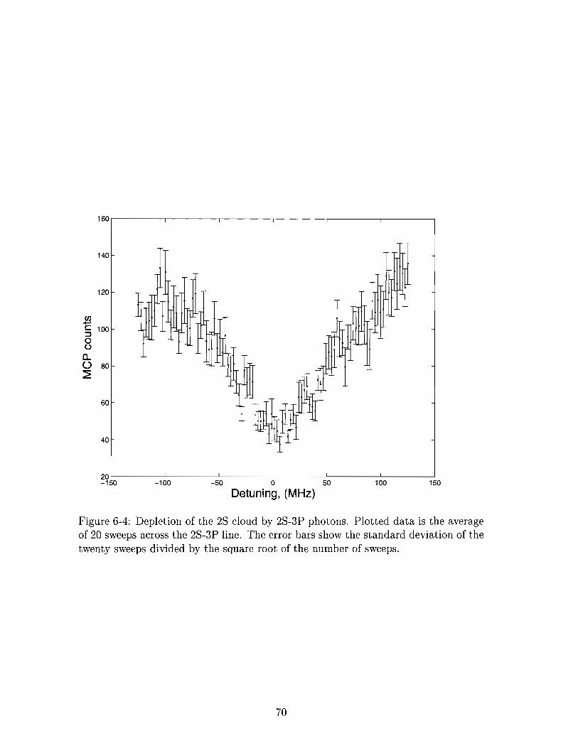
201 I I I I I I
-1 50 -1 00 -50 0 50 100 150
Detuning, (MHz)
Figure 6-4: Depletion of the 2s cloud by 2s-3P photons. Plotted data is the average of 20 sweeps across the 2s-3P line. The error bars show the standard deviation of the twenty sweeps divided by the square root of the number of sweeps.
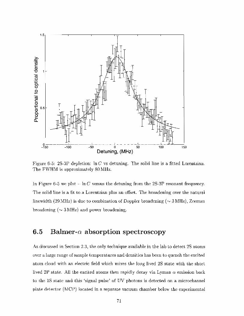
Figure 6-5: 2s-3P depletion: 1nC vs detuning. The solid line is a fitted Lorentzian. The FWHM is approximately 80 MHz.
In Figure 6-5 we plot - In C versus the detuning from the 2s-3P resonant frequency.
The solid line is a fit to a Lorentzian plus an offset. The broadening over the natural
linewidth (29 MHz) is due to combination of Doppler broadening (N 3 MHz), Zeeman
broadening ( N 3 MHz) and power broadening.
Balmer-a absorption spectroscopy
As discussed in Section 2.3, the only technique available in the lab to detect 2s atoms
over a large range of sample temperatures and densities has been to quench the excited
atom cloud with an electric field which mixes the long lived 2s state with the short
lived 2P state. All the excited atoms then rapidly decay via Lyman a emission back
to the 1s state and this 'signal pulse' of UV photons is detected on a microchannel
plate detector (MCP) located in a separate vacuum chamber below the experimental
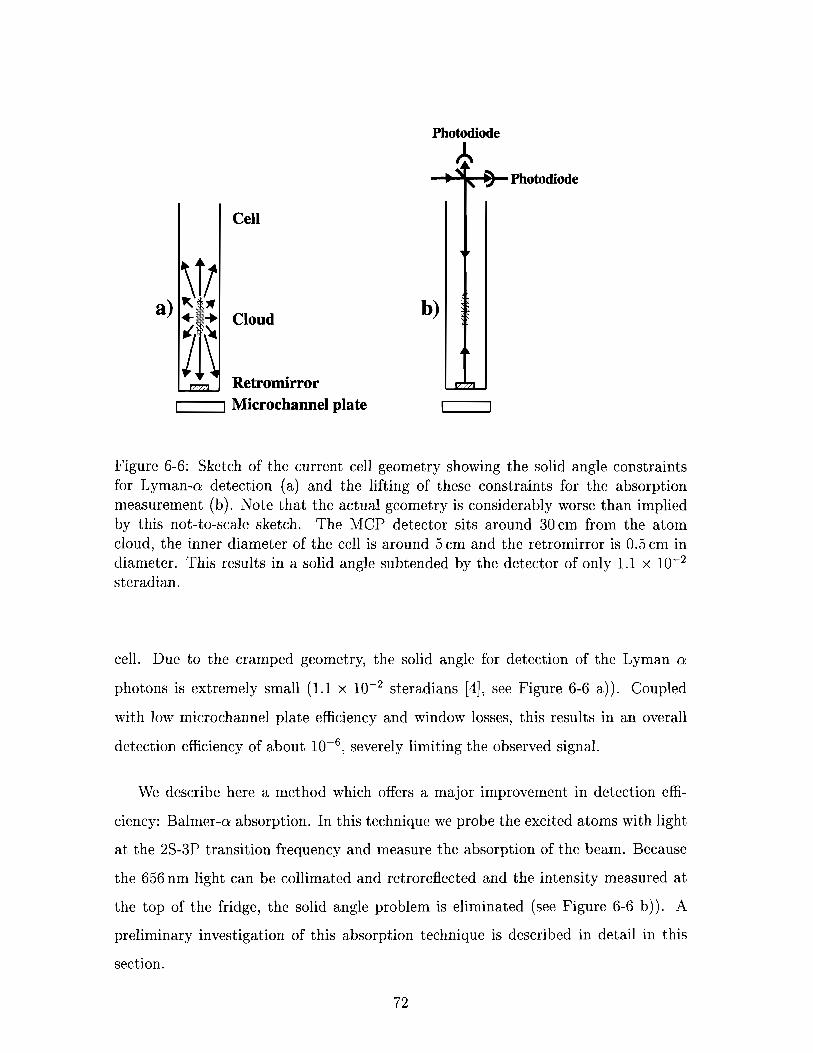
Photodiode
Cell
Cloud
Retromirror 1-1 Microchannel plate
I Pho todiode
Figure 6-6: Sketch of the current cell geometry showing the solid angle constraints for Lyman-a detection (a) and the lifting of these constraints for the absorption measurement (b). Note that the actual geometry is considerably worse than implied by this not-to-scale sketch. The MCP detector sits around 30 cm from the atom cloud, the inner diameter of the cell is around 5 cm and the retromirror is 0.5 cm in diameter. This results in a solid angle subtended by the detector of only 1.1 x steradian.
cell. Due to the cramped geometry, the solid angle for detection of the Lyman a
photons is extremely small (1.1 x steradians [4], see Figure 6-6 a)) . Coupled
with low microchannel plate efficiency and window losses, this results in an overall
detection efficiency of about lov6, severely limiting the observed signal.
We describe here a method which offers a major improvement in detection effi-
ciency: Balmer-a absorption. In this technique we probe the excited atoms with light
at the 2s-3P transition frequency and measure the absorption of the beam. Because
the 656 nm light can be collimated and retroreflected and the intensity measured at
the top of the fridge, the solid angle problem is eliminated (see Figure 6-6 b)). A
preliminary investigation of this absorption technique is described in detail in this
section.

6.5.1 Overview
The expected signal is a reduction in the number of red photons making it through
t:he atomic c:loud when the UV laser is tuned to resonance with the 1S-2s transition.
After trapping and cooling 1s hydrogen, we promoted a small fraction to the 2 s state
via the absorption of two UV photons. To search for an absorption signal, we first
located the 2S-3P resonance by sweeping the red laser across the expected transition
frequency (as in the experiments described in Section 6.4). In subsequent traps we
held the red light frequency fixed while sweeping the UV frequency across the 1S-2s
line. The advantage of sweeping the UV rather than the red is because the relative
stability of the 2S-3P laser is much better than the 1S-2s laser. Once the 2S-3P
laser is locked, its frequency will stay close to the center of the resonance for many
hours. By comparison, the UV laser would need to be re-centered every half an hour
or so. The experimental cycle at each UV frequency point is shown in Figure 6-7. An
electrical quench is used to remove the remaining 2 s atoms before the next cycle.
6.5.2 Absorption setup
A schematic of the fridge top optical setup for the absorption measurement is shown
in Figure 6-8. The 656nm light is transported to the fridge top in a single mode
optical fiber [24]. Smooth power control is provided via a polarizing beam splitting
cube and a half-wave plate. There is some evidence of power drift over the course of
a day which is likely due a t least in part to drift of the output polarization from the
fiber. This could be controlled if necessary but has not limited our experiments so
far.
After the polarization optics, the 656 nm light is reflected from a glass slide. The
tra'nsmitted light is collected on a photodiode while the 4% reflection is sent into a
beam shaping telescope. The beam then propagates down through the cryostat and
the trapping cell and is retroreflected with very high efficiency a t the cell bottom
mirror. The retroreflected beam passes through the atom cloud again and exits the
cryostat a t the fridge top window. At the glass slide, the majority of the retroreflected

Trap and cool 1s hydrogen
/
Make metastable Quench to remove remaining 2s atoms
Excite 2s-3P transition
Figure 6-7: Spectroscopy cycle for 2s-3P absorption experiments. The 1s hydrogen cloud acts as a reservoir of cold atoms.

Adjustable fiber launcher
11
Polarizing beam splitter
Glass slide
Avalanche photodiode Thorlabs DET-110 monitoring return power monitoring in-going
power
Figure 6-8: Optical setup for 656 nm absorption measurement. Smooth power control is provided via t'he half wave plate and the polarizing beam splitter.
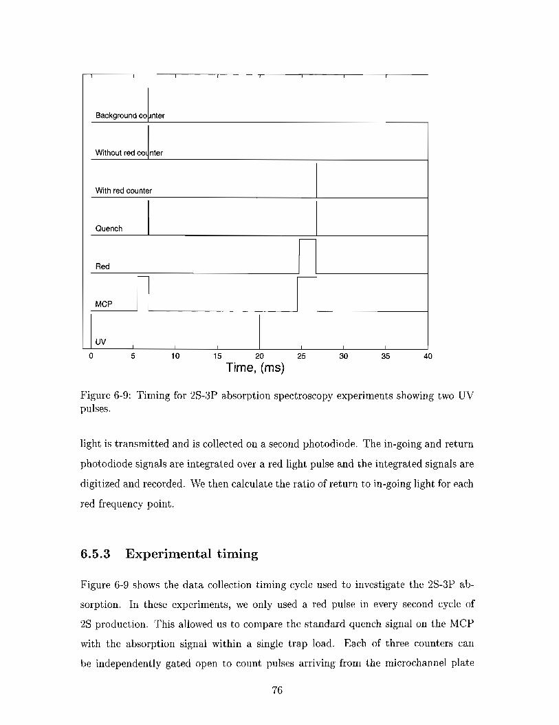
0 5 10 15 20 25 30 35 40
Time, (ms)
I I I I I I I I
Figure 6-9: Timing for 2s-3P absorption spectroscopy experiments showing two UV
Background co
Without red coi
pulses.
~nter
nter
light is transmitted and is collected on a second photodiode. The in-going and return
photodiode signals are integrated over a red light pulse and the integrated signals are
digitized and recorded. We then calculate the ratio of return to in-going light for each
red frequency point.
6.5.3 Experimental timing
With red counter
Quench -
Red I
MCP
Figure 6-9 shows the data collection timing cycle used to investigate the 2s-3P ab-
sorption. In these experiments, we only used a red pulse in every second cycle of
2s production. This allowed us to compare the standard quench signal on the MCP
with the absorption signal within a single trap load. Each of three counters can
be independently gated open to count pulses arriving from the microchannel plate
uv I I I I I I
stack. The background counter is open for 80 ps directly before the quench pulse.
The quench plates are energized for 40ps. The with-red and without-red counters
are open during alternate quench pulses. 40 ps has been experimentally shown to be
a good compromise between a high percentage of atoms quenched and a reasonable
background noise level in the observed counts. The MCP is switched on a consider-
able time before the quench to allow the stack to warm up and reach full detection
efficiency. The difference in MCP on-time between the red and no-red cycles is a
quirk of the timing simulator and has no impact on the experiment. In the prelimi-
nary signal search presented here, we used a pulse length of 1 ms. Even if the beam
intersected with only a portion of the cloud, with a 1 ms pulse length and a radial
trap frequency of 1 kHz we expected that a reasonable number of the atoms would
pass through the laser beam during the light pulse due to their motion through the
trap.
6.5.4 Power requirements
To search for an absorption signal, we need an estimate of the light intensity required.
For a one-photon transition such as the 2s-3P, the saturation intensity is given by [25]
where I? = l/rnat and wo is the resonant frequency. Rewriting this in terms of more
useful quantities [26] we have
where T is the excited state lifetime and X is the resonant wavelength. For 2s-3P, we
have 7-3p = 1/(27~ x 30 MHz) = 5.3 ns and X = 656 nm so Isat = 13.9 mW/cm2. For
a 100 pm diameter beam waist, we reach the saturation intensity with just 1 p W of
656 nm power.
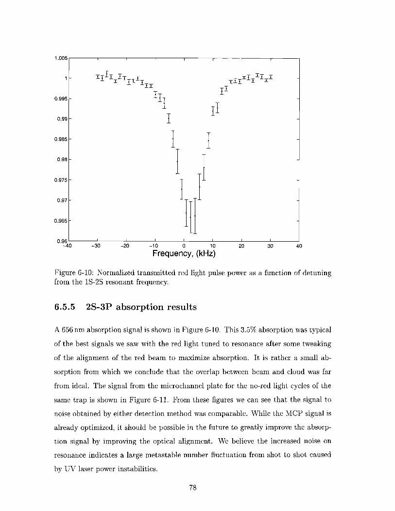
0.96' I I I I I I i I
-40 -30 -20 -1 0 0 10 20 30 40
Frequency, (kHz)
Figure 6-10: Normalized transmitted red light pulse power as a function of detuning from the 1s-2s resonant frequency.
6.5.5 2s-3P absorption results
A 656 nm absorption signal is shown in Figure 6-10. This 3.5% absorption was typical
of the best signals we saw with the red light tuned to resonance after some tweaking
of the alignment of the red beam to maximize absorption. It is rather a small ab-
sorption from which we conclude that the overlap between beam and cloud was far
from ideal. The signal from the microchannel plate for the no-red light cycles of the
same trap is shown in Figure 6-11. From these figures we can see that the signal to
noise obtained by either detection method was comparable. While the MCP signal is
already optimized, it should be possible in the future to greatly improve the absorp-
tion signal by improving the optical alignment. We believe the increased noise on
resonance indicates a large metastable number fluctuation from shot to shot caused
by UV laser power instabilities.

Figure 6-1 1: The traditional Lyman-a signal collected for the same trap as Figure 6- 10. The ordinate is the detuning of the UV frequency from the 1s-2s resonance. The co-ordinate is th.e average number of 2s counts per scan across the resonance.
120.
100
80
v, * LZ 3 60
S 40
20
0 -30 0 10 20 30
Frequency, (kHz)
- I I I 1
-
-
ll1, -
- I 1 1 -
-
I I I -
- ,I I -
I I
1 I== =I , I T ~ I : T I
=IT ==XIXI
- I I I I I
-20 -1 0
-
This trap used the timing cycle described in Section 6.5.3 with a 1 ms red pulse
length. The input red power measured at the fridge top window was 120nW. The
return power off resonance was around 50 nW. The loss is dominated by the uncoated
optics in the laser path within the cryostat.
6.5.6 Calculation of metastable number produced
If the signal from the MCP is the only method of 2s atom detection, there is no way
to make a direct calculation of the absolute number of 2s atoms excited. Previous
values rely on an estimate of the efficiency of Lyman a detection [4]. Combining the
MCP data with data from our Balmer-a absorption spectroscopy offers a more direct
measurement of metastable number. Knowledge of the absolute 2s atom number and
hence the 2s atom density will be useful in our proposed precision measurements of
other transition frequencies in hydrogen (see Chapter 7) both in the design of the
experiments and in the interpretation of results.
From the data presented in Figures 6-10 and 6-12, we can estimate the number
of metastable 2s atoms produced for a single UV laser shot. First let us define A,
the fractional absorption of the red light on resonance and D, the observed fractional
depletion of the metastable atoms on resonance. We then further define the light
power reaching the atoms for an input power at the cell top window of P as,
where T takes into account the less than perfect transmission at each of six uncoated
glass surfaces between fridge top and atom cloud (two each from the fridge top win-
dow, the blackbody window and the cell top lens). For a pulse of length t we have
N,, the number of photons reaching the cloud given by,
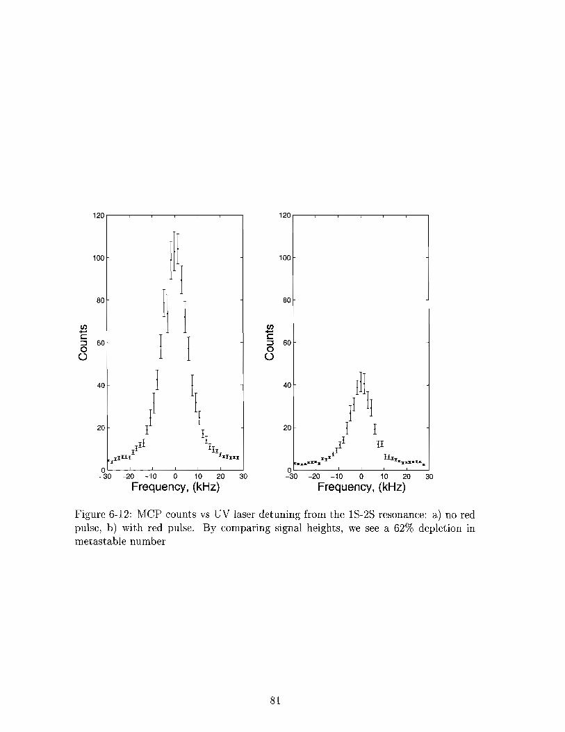
Figure 6-12: MCP counts vs UV laser detuning from the 1s-2s resonance: a) no red pulse, b) with red pulse. By comparing signal heights, we see a 62% depletion in metastable number

Table 6.1: Parameters for metastable number calculation with estimated errors.
where E, is the energy of a single photon. Hence the number of photons absorbed is
and the number of 2s atoms is given by
The parameters and estimated errors are given in Table 6.1. The resulting estimate
for the 2s atom number created by a lms pulse of UV light on resonance with 1s-2s
All the errors could be reduced in a more careful and deliberate measurement. T can
be bought extremely close to one by replacing the fridge optics with versions which
are AR coated at 656nm. With this simple formalism, we now have a method to
calculate the metastable number produced for any given cloud geometry, UV laser
parameters, etc.
We can also combine this metastable number calculation with the observed number
of microchannel plate counts to get an estimate of the MCP detection efficiency. Note
that because the timing simulator was run twice before readout, the accumulated
MCP counts a t each frequency are actually for two UV laser pulses. Given that we
saw around 100 f 15 Lyman-cu counts on the microchannel plate this implies that 18

million 2s a,toms resulted in 50 f 8 Lyman-a counts giving a detection efficiency of
2.9 x 5 0.1 x in reasonable agreement with the earlier estimate of 1.9 x f
0.8 x lov6 [4]. For any given MCP geometry and cell construction, this technique
gives a simple method for calibrating the observed 2s atom number.
6.6 Detection methods for metastables
One of the prilnary motivations for pursuing 2s-3P spectroscopy was to investigate
using absorption of 2s-3P photons as a probe of the metastable cloud. The experi-
ments in this thesis have demonstrated this absorption signal in trapped metastable
hydrogen for the first time. In this section we consider the signal-to-noise ratio that
can be expected from the two different detection methods - MCP detection and
Balmer-a absorption.
6.6.1 Expected signal-to-noise ratio from MCP
We want to measure the number of 2s metastable atoms at a given time after they
are excited. This is done by quenching the metastables with an applied electric field
and counting the Lyman-a decay photons. Let No be the number of metastables and
t'he detection efficiency. Then the number of detected atoms is Nd = €NO, and the
total number of counts from the MCP detector is
where Ns is t'he number of background counts on the detector. NB is given by the
product of the average background rate and the detection gate time, typically 40 ps.
Assuming stakistical noise, the variance in C is given by 06 = C. We will use the
estimator

The signal is No. The noise on the observed counts on resonance is given by
Hence
Figure 6-13 shows the signal-to-noise ratio vs metastable number for a single quench
cycle with 6 = 1 x (about that expected for the MCP stack geometry in the
new hydrogen apparatus), a background of 100000 counts per second (typical of the
background noise observed in the old apparatus) and a quench time of 40 ps.
6.6.2 Expected signal-to-noise ratio from absorption
The aim of this section is to demonstrate that in certain regimes the signal-to-noise
ratio that can be expected from the absorption method greatly exceeds that for the
MCP detector. We will consider a simple model for absorption which neglects multi-
photon processes. These processes only become significant as the intensity of the light
beam approaches the saturation intensity. We will also neglect the atoms that fall
back into the 2s state from 3P1. Because we want to consider situations where the
number of metastable atoms and the number of photons in the light pulse are roughly
similar, the absorption can be large. In this case it is important to realize that the
optical density of the sample changes during the length of the absorption pulse and
that the intensity of the light beam changes from one end of the cloud to the other.
Consider a collection of atoms of scattering cross section o in a cylinder with
radius R and length L and imagine a detector behind the atom cloud of area .rrR2.
The laser beam radius is matched to the cloud size. The probability that a photon
'The branching ratio for decay of 3P atoms to the 2s state compared to the ground state is around 8%

Figure 6-13: Signal-to-noise ratio vs metastable number for a single quench cycle for the MCP stack using typical operating conditions: 6 = 1 x and NB = 4.

makes it through the cloud, which is equal to the probability that it falls on the
detector, is given by
where p = ~ / T R ~ for notational convenience. Hence the probability that it does not
fall on the detector, which is equal to the probability that an atom is removed, is
If k is the number of photons incident on the cloud, in the limit of a large number of
atoms we can make the approximation that
where Nk is the number of metastable atoms surviving after k photons. Rewriting in
integral form we have the following expression for Nk,
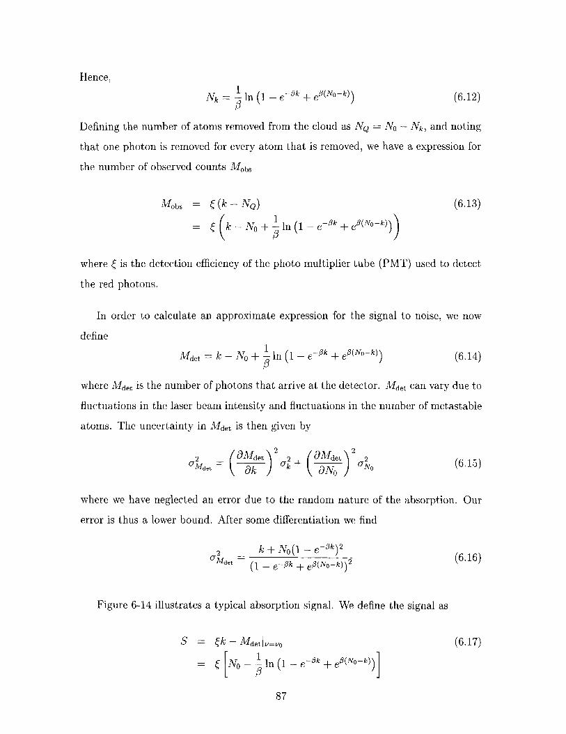
Hence,
Defining the number of atoms removed from the cloud as NQ = No - Nk, and noting
that one photon is removed for every atom that is removed, we have a expression for
the number of observed counts Mobs
Mobs = E (k - NQ) (6.13) 1 k - N~ + - In (1 - e-Bk + eP(N~-k) P
where < is the detection efficiency of the photo multiplier tube (PMT) used to detect
the red photons.
In order to calculate an approximate expression for the signal to noise, we now
define
where Mdet is the number of photons that arrive at the detector. Mdet can vary due to
fluctuations in the laser beam intensity and fluctuations in the number of metastable
atoms. The uncertainty in Mdet is then given by
where we have neglected an error due to the random nature of the absorption. Our
error is thus a lower bound. After some differentiation we find
Figure 6-14 illustrates a typical absorption signal. We define the signal as

Figure 6-14: Sketch of typical absorption signal showing definition of signal and contributions to the noise (shaded area).

As an approximation for the noise we will take
= lo^,., I b,, + Ek
where (k is the noise contribution from the baseline and oLdet = <oLObs.
This model is valid only for an operating regime where the intensity is smaller
than Isat. This places an upper limit on the minimum pulse length required to deliver
a given number of photons2. Previously we have calculated Isat to be 13.9 mW/cm2
or 139 W/m2. With an energy per photon of E, = 3.03 x lo-'' J this translates to
Isat = 4.59 x 1(120 photonso s-'rnM2. Hence if we deliver lo8 photons into an area of
ra,dius 100 prn with a pulse length of 1 ms then I / Isat is only 7 x
A short pulse is desirable to minimize background noise. However for a PMT, this
noise can be extremely low. If the noise counts are a few per second, in a measurement
interval of a millisecond they will be completely negligible compared to the shot noise
errors caused by photon counting.
To produce the plots in this section, we have taken the quantum efficiency for
extended red range PMT at 656nm as [ 5%, the area of the cloud to be n x
(100 pm)2 and o = 2.4 x 10-lo cm2 [4]. The signal-to-noise ratio is plotted in Figure 6-
15 for a range of metastable sample sizes and a fixed number of input photons, k = lo7.
We will consider the nature of the observed absorption signals for peak on resonance
metastable sample sizes in the regions around I, I1 and 111.
At I, the signal is atom limited. All the atoms are lost and the signal increases
linearly with the number of metastable atoms. The noise comes in roughly equal parts
from fluctuations in the signal and in the baseline and is approximately proportional
to with little dependence on metastable number.
At 111, the signal is photon limited. On resonance, all the photons are absorbed.
We also note a practical limit on the shortest pulse used. The length of the light pulse r656 is best controlled using an AOM. For a 200 MHz AOM with a 0.1 mm diameter beam, the rise time of the light pulse is on the order of 20ns. Hence a reasonable value for the minimum length pulse is around 100ns from a technical stand point.

Figure 6-15: Signal-to-noise ratio for 2S-3P absorption for 10 million input photons
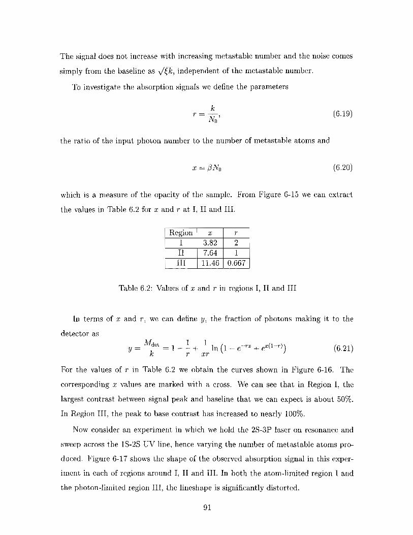
The signal does not increase with increasing metastable number and the noise comes
simply from the baseline as G, independent of the metastable number.
To investigate the absorption signals we define the parameters
the ratio of the input photon number to the number of metastable atoms and
which is a rnea,sure of the opacity of the sample. From Figure 6-15 we can extract
the values in Table 6.2 for x and r at I, I1 and 111.
Table 6.2: Values of x and r in regions I, I1 and I11
In terms of x and r , we can define y, the fraction of photons making it to the
detector as
For the values of r in Table 6.2 we obtain the curves shown in Figure 6-16. The
corresponding x values are marked with a cross. We can see that in Region I, the
largest contrast between signal peak and baseline that we can expect is about 50%.
In Region 111, the peak to base contrast has increased to nearly 100%.
Now consider an experiment in which we hold the 2s-3P laser on resonance and
sweep across tlhe 1s-2s UV line, hence varying the number of metastable atoms pro-
duced. Figure 6-17 shows the shape of the observed absorption signal in this exper-
iment in each of regions around I, I1 and 111. In both the atom-limited region I and
the photon-limited region 111, the lineshape is significantly distorted.
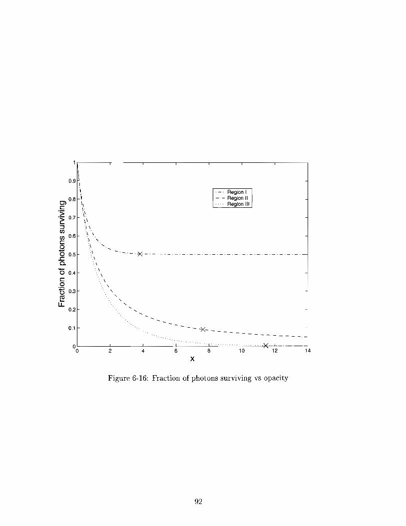
Region I Region II Region Ill
X
Figure 6-16: Fraction of photons surviving vs opacity
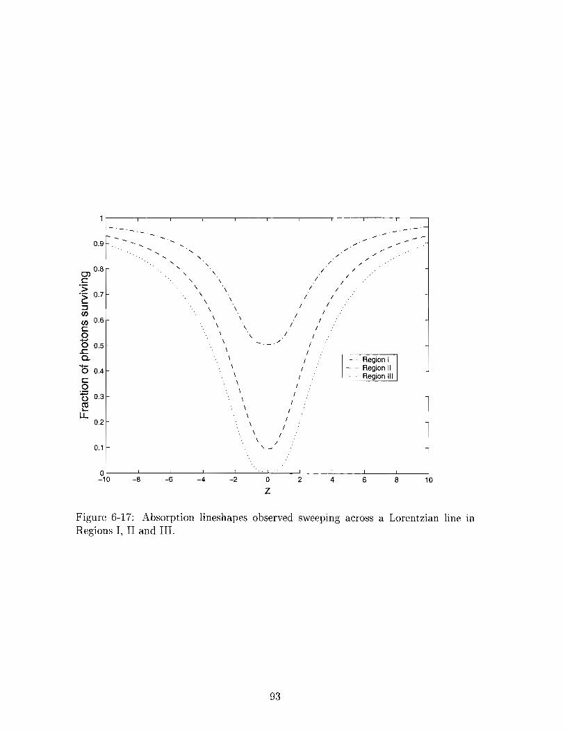
Region I Region 11
Figure 6-17: Absorption lineshapes observed sweeping across a Lorentzian line in Regions I, I1 and 111.

1 o - ~ I I I I I I I I I 0 10 20 30 40 50 60 70 80 90 100
2s atom number (millions)
Figure 6-18: Signal to noise comparison: MCP (solid line) vs absorption (dots and dashed line)
6.6.3 Signal- to-noise ratio comparison
As can be seen from Section 6.6.2, absorption detection is significantly more compli-
cated than MCP detection and optimizing the signal-to-noise ratio observed would
depend on a knowledge of the application. To illustrate the advantages of the ab-
sorption method in at least one instance, in this section we consider the case where
r is always held at one i.e. the peak number of metastable atoms is the same as the
average photon number. In this region (11) we expect to see a line shape with only
modest distortion. As illustrated in Figure 6-18, the gain in expected signal-to-noise
ratio operating in this regime is very significant. We note that while designing a shot-
noise limited detection system for 656 nm photons would be challenging, even without
reaching this limit absorption spectroscopy offers a real possibility for improvement
over the previously used MCP detection.

Chapter 7
Proposed spectroscopy of the
2S-8s transition
This chapter discusses the proposed high precision measurement of the 2S-8s fre-
quency in our trapped atomic hydrogen sample. Problems with the cryogenic side of
the apparatus have so far frustrated our attempts to complete these experiments. The
laser systems have been designed, constructed and tested but the atomic hydrogen
sample is sadly absent. When the new hydrogen trapping apparatus comes on line, a
search for the 2S-8s line can be undertaken.
7.1 Motivation
7 .11 Why a precision frequency measurement?
The main goal of a high precision measurement of the hydrogen transition frequencies
is to allow a closer comparison of the predictions of theory with the observations of
experiment. Specifically, we want to extract from our frequency measurements a value
for the Rydberg constant and for the 1s Lamb shift. While an outstandingly precise
measurement has been made of the 1S-2s frequency that brings the uncertainty to
1.8 parts in 1014 [27], the frequency of at least two transitions must be known in
order to extract QED or nuclear effects. If v ( l S - 2 s ) is taken as one frequency,
the ultimate precision of the theory-experiment comparison is currently limited by
the experimental knowledge of the second frequency. Hence our goal to perform a
precision measurement of the 2s-8s transition frequency. The current record for this
measurement is held by the group of Franz Biraben in Paris [28-311.
7.1.2 Why in trapped hydrogen?
Precision measurements in hydrogen have a long history (see Chapter 1) and are still
an active field. Hence we will briefly explain why we believe that the MIT Ultracold
Hydrogen experiment has the potential to produce a significant improvement on a
measurement of the 2s-nS frequencies.
All other 2s-nS experiments with hydrogen [28] make use of an atomic beam where
the 2s atoms are created by electronic bombardment. The most probable velocity
for the metastable atoms is around 4000ms-'. Optical production of our 2s sample
from a trapped 1s cloud at 100 pK via a UV laser creates a trapped 2s sample in
which the most probable velocity is around 1.6 ms-l. The cold, confined cloud allows
for an extended interaction time of the atoms with the laser light, with the potential
to greatly reduce the required light intensities and hence the errors due to the AC
Stark effect. Additionally the second order Doppler shift is negligibly small. The
AC Stark shift and the second order Doppler shift contributed the limiting errors
in previous experiments [28]. It is also important to note that because of Zeeman
effects (see Section 7.6.3) measurements in a magnetically trapped hydrogen sample
are restricted to S to S transitions. These and other systematic errors are studied in
more detail in Section 7.6.
Our ability to make a direct, real time comparison of the 1s-2s and 2s-8s fre-
quencies via the femtosecond comb should also yield an appreciable improvement in
the error of the frequency measurement (currently a 2 kHz contribution to the final
frequency error in [28]). Importantly, because we excite the 1s-2s transition to create
our atoms, we have a natural frequency reference in terms of the best known optical
transition. This advantage, combined with the femtosecond comb and the ultracold
hydrogen should permit a major advance. (For more details see [32].) An added

Table 7.1 : 2s-nS transition wavelengths. Two photons are required for each transition.
Transition 2s-4s 2s-6s 2s-8s 2s-10s 2s-12s
advantage is that ultimately any n level is accessible because the frequency reference
is the comb rather than some frequency specific laser chain.
Wavelength ( nm) 972.53 nm 820.57 nm 778.03 nm 759.79 nm 750.24 nm
7.1.3 Why 2s-8S?
As mentioned in Section 7.1.2, in a magnetic trap we are restricted to measurements
from 2s to higher nS levels. Table 7.1 shows the wavelength for each of the two
photons required to pump a 2s-nS transition for a range of n. In the long term,
we would like to measure the frequencies of several transitions. A number of factors
influenced our clioice of 2s-8s as the initial transition. The natural linewidth decreases
as approximately l /n3 for n > 2. Hence a higher excited state presents a narrower
line. However the Stark effects due to static electric fields increase rapidly with
increasing n (as n7 for the shift due to the quadratic Stark effect) so higher order
n states are increasingly vulnerable to stray electric fields. These two ideas taken
together suggest a moderately high n state as a good first choice. From the point of
view of an experimental implementation, for the states with n 2 6, 2s-8s lies closest
to the free running wavelength of a commercially available diode laser.
7.2 The Rydberg constant
7.2.1 History
Some years after Balmer's work showing that the many wavelengths of transitions in
the hydrogen atom then observed could be represented by a simple formula, Johannes

Rydberg developed a formula which could accurately predict not only the spectra of
hydrogen but the observations of the wavelength series apparent in the spectra of
many chemical elements. When he discovered Balmer's paper, Rydberg realized that
its predictions could be recast in the same form as his own more general formula to
give,
R, was first experimentally determined in 1890 by Rydberg with an accuracy of
better than 1 part in lo3.
As it stood, the Rydberg was merely an empirical number. In 1913, however, Neils
Bohr's theory for the hydrogen atom provided the Rydberg with a theoretical basis
so that he was able to calculate its value in terms of other fundamental quantities:
the electron mass (m), the electron charge (e), the velocity of light (c) and the Planck
constant (h),
The Rydberg, or more precisely, hcR,, was then revealed as the natural energy scale
of atomic physics. It is basic to all calculations of atomic and molecular energy lev-
els and is important in many areas of physics and chemistry. Optical spectroscopy
brought the accuracy to 1 part in lo7 by the 1970s. In 1974, Theodor Hansch in-
troduced laser spectroscopy of hydrogen, using saturated absorption spectroscopy to
eliminate Doppler broadening. Laser spectroscopy in hydrogen has since improved
the results to the point where the uncertainty is a mere 7.7 parts in 1012 [28] mak-
ing the Rydberg constant currently the most precisely measured of all fundamental
physical constants.
7.2.2 Significance of a new measurement
A quantity is considered fundamental if its value comes from a core theory of physics
and determines the magnitude of a basic interaction of nature. A fundamental con-
stant is linked to other constants and helps to establish values of other significant
quantities. The fundamental constants are often needed in comparisons between ex-

periment and theory and, if known to high precision, can play a role in exposing the
strengths and weaknesses of a particular theory. Efforts to measure the fundamental
constants with ever increasing accuracy have resulted in new experimental techniques
which continue to pay dividends throughout science. The Rydberg constant is cur-
rently so well known that the significance of any further improvement is in large part
the contribution of the work to extending the art of spectroscopy and high precision
measurement.
7.3 The Lamb shift
7.3.1 History
In June 1947, soon after the end of World War 11, a physics conference was held on
Shelter Island, New York. Most of the conference participants had recently returned
to academic life after working for several years on war-related projects such as de-
veloping rada.r systems at MIT or at the top secret Manhattan project designing the
atomic bomb a t Los Alamos. On the first day of the conference, Willis Lamb pre-
sented new experimental data on the spectrum of the hydrogen atom that exposed a
discrepancy with Dirac theory [33]. Dirac had predicted that the states of hydrogen
with n = 2, J = 112 would be degenerate in energy. In an experiment using a radio
frequency resonance technique, Lamb measured an energy gap of 1050 f 10 MHz be-
tween 2S112 and 2Plj2. The precision of this experiment at around 1% was hundreds
of times better than the best that had been achieved optically and left little doubt
that a major shake-up of atomic theory was about to occur. It was this discovery of
the Lamb shift which led to the description of physical processes via quantum field
theory.
Although the original Lamb shift is the energy gap between the 2SlI2 and 2Pllz
levels, it is now common practice to refer to any energy gap between nSl12 and nPl12
levels as a Lamb shift. In this nomenclature, Lamb's original shift becomes the 2s
hydrogen Lamb shift or in this thesis where only hydrogen is discussed, the 2s Lamb

shift.
7.3.2 Dissecting the Lamb shift
The hydrogen energy levels can be expressed as
where R, is the Rydberg constant and a is the fine structure constant. EHFs denotes
the contribution from the hyperfine structure.
The Lamb shift, hL(n, J, L) contains all the QED corrections and corrections for
the finite size and polarizability of the nucleus and can be written as [34]
where
F, is the expression for an infinitely heavy point nucleus and can be expanded as
where Apq and Bpq are dimensionless constants depending on the quantum numbers
L, J and sometimes n . Terms in Apq are the so called one-loop corrections associated
with self-energy and vacuum polarization where the corresponding Feynman diagrams
have only one loop. Terms in Bpq correspond to two-loop diagrams. These two loop
corrections have recently been the subject of much theoretical interest because of
calculations showing "a peculiar behavior which may significantly alter the theoretical
predictions for low lying states" [35].
FRR and FNR in Eqn 7.4 refer to corrections for a nucleus of finite mass, account-
ing for the radiative and non-radiative nuclear recoil motion respectively. FpOl is a
correction for the finite polarizability of the nucleus [36].

FNS is a correction for the shift caused by finite nuclear size. This can be calculated
in non-relativistic perturbation theory as
where p is the reduced mass, re = a2ao is the classical electron radius and r, is the
proton charge radius. The accuracy of the current experimental determination of the
proton charge radius is of considerable importance in the comparison of any Lamb
shift measurem.ent with calculations of hydrogen structure using bound state QED
theory (see Section 7.3.3).
7.3.3 Significance of a new measurement
Because of the tremendous advances in optical spectroscopy over the last few decades,
Lamb shift measurements in hydrogen have now reached the point where the interpre-
tation of results is affected by the finite size of the proton. Current knowledge of the
proton charge radius comes from traditional electron scattering measurements [37-
401. Unfortunately, these experiments are difficult to perform and the analysis of
results is complicated. An alternative approach is currently being pursued at the
Patul Scherrer Institute in Switzerland [41]. A collaboration is preparing to measure
the 2s Lamb shift in muonic hydrogen: a hydrogen-like atom where the electron is
replaced by the much heavier muon (m,,,, x 207m,). Due to the small Bohr ra-
dius, the nuclear size effects have a significantly larger effect on the energy levels of
muonium. A determination of the proton charge radius to a part in lo3 should be
possible from a measurement of the 2S-2P splitting. This would improve the current
situation by more than an order of magnitude.
If such an improvement is made in the knowledge of the proton charge radius, the
bulk of the experimental uncertainty in the hydrogen Lamb shift would shift back to
the knowledge of the transition frequencies. An improvement in the 2S-8s transition
frequency would then allow a closer comparison between experiment and QED theory.

7.4 Current measurement precision
The current best measurements of the 2s-nS transition frequencies in hydrogen are
those made by Franz Biraben and collaborators in Paris [28-311. These experiments
were carried out in a metastable atomic beam formed by electronic bombardment of
a beam of 1s atomic hydrogen. The reported frequency for the 2s-8s transition is
an accuracy of around one part in 10" [28]. By combining this measurement with
further, similarly accurate measurements of the 2 s - 8 0 and 2 s - 12S, D transition
frequencies, the highly accurate experimental value of v ( l S - 2 s ) [27] and some
theoretical calculations for differences between Lamb shifts [42], de Beauvoir et a1 [28]
extract
R, = 109737.31568550(84) cm-',
L(1S) = 8172.840(22) MHz,
L(2S) = 1057.8450(29)MHz.
currently the most precise values available.
7.5 Proposed experiment
The limiting errors in previous experiments have been the AC Stark shift and the
second order Doppler shift [28]. As discussed in Section 7.1.2 because of our cold
atoms and increased interaction times, we believe we can improve upon the current
experimental accuracy of the 2s-8s transition. The structure of the proposed ex-
periment is as follows. After trapping and cooling a reservoir of atomic hydrogen in
the 1s Id) state (see Section 2 4 , a metastable population of atoms in the 2s state
is created using a UV laser (see Section 2.2). These metastables are quenched us-
ing an applied electric field and the resulting Lyman-a photons are counted with a
microchannel plate (see Section 2.3). This measurement gives a base line count for
the number of metastables produced. In the next cycle of 2s production, the atoms
are also illuminated with a laser at half the two-photon 2s-8s transition frequency
which excites the 2s atoms up to the 8 s state. The majority of these atoms decay by
radiative cascade into the ground state. After some laser on time, the metastables
are again quenched and the remaining 2 s atom number is detected. The depletion in
the number of metastable atoms is then recorded as the 2s-8s laser is swept through
resonance. The expected signal is similar to the depletion spectra observed in our 2s-
3P experiments (see Figure 6-4). This depletion must then be fit to some calculated
lineshape and the corrected center frequency extracted.
At each frequency point in the depletion measurement, the frequency of the 2s-8s
laser is measured relative to the frequency of the 1s-2s laser which is exciting the
metastables. The two laser frequencies are linked via a femtosecond, mode-locked
Ti:Saph comb. Further details of the frequency measurement will be covered in 1321.
7.6 Systematics
This section contains a brief discussion of the expected sources of shifts and broaden-
i n g ~ of the 2s-8s transition in a trapped hydrogen sample and contrasts them with
the errors observed in the hydrogen beam experiment. While a shift or broadening
can be compensated for to some extent in the data analysis and lineshape calcula-
tion, the smaller the effect, the smaller will be the residual error. For comparison,
the natural linewidth of the 2s-8s transition at 778 nm is 72 kHz.
7.6.1 DC Stark effect
From [28] we have that the 2s-8s transition has a shift due to small electric fields of
strength E of

For a stray electric field of 40 mV/cm (the upper limit on the stray electric fields
of the old hydrogen trapping cell as estimated in [4]) this gives a shift of 143 kHz.
This is a significant shift and one which is hard to remove accurately in data analysis
because the magnitude of the stray fields are difficult to measure. In the hydrogen
beam experiments, the stray fields were estimated at 3 mV/cm and were calculated
to contribute a frequency uncertainty of 0.4 kHz. In a new cell designed specifically
for precision measurement, it will be worthwhile to make a concerted effort to reduce
the stray fields (see Section 9.1.2).
7.6.2 AC Stark effect
The total two-photon transition probability scales as 12tint where tint is the interaction
time of the light with the atoms. The AC Stark effect, however, is linear in the
intensity. If we increase tint, we can decrease I and therefore decrease the light shift.
In the atomic beam experiments, where the interactions times were around 200 ,us,
the required peak intensities1 were - 1.5 x lo8 W/m2 causing light shifts of around
400 kHz. By repeating the measurements at a series of light powers and extrapolating
to zero light power, the center frequency of the unshifted line was extracted with an
error of around 7 kHz [28]. In a measurement in trapped hydrogen we can expect
interaction times two orders of magnitude longer (see Section 7.7). Hence the required
intensities can be around ten times lower bringing the light shift down to 40 kHz. With
a similar effort in error analysis, the residual error due to the light shift should be
reduced to less than 1 kHz. There will also be some broadening due to the variation of
light intensity seen by the atoms in the trap. This effect would need to be convolved
into the lineshape calculation as is done for the beam experiments.
'Quoted intensities will be given as the peak intensity for a Gaussian beam i.e. I =
for x = y = t = 0 where w, = w o J m and zo = ?rwi/X is the Rayleigh range.
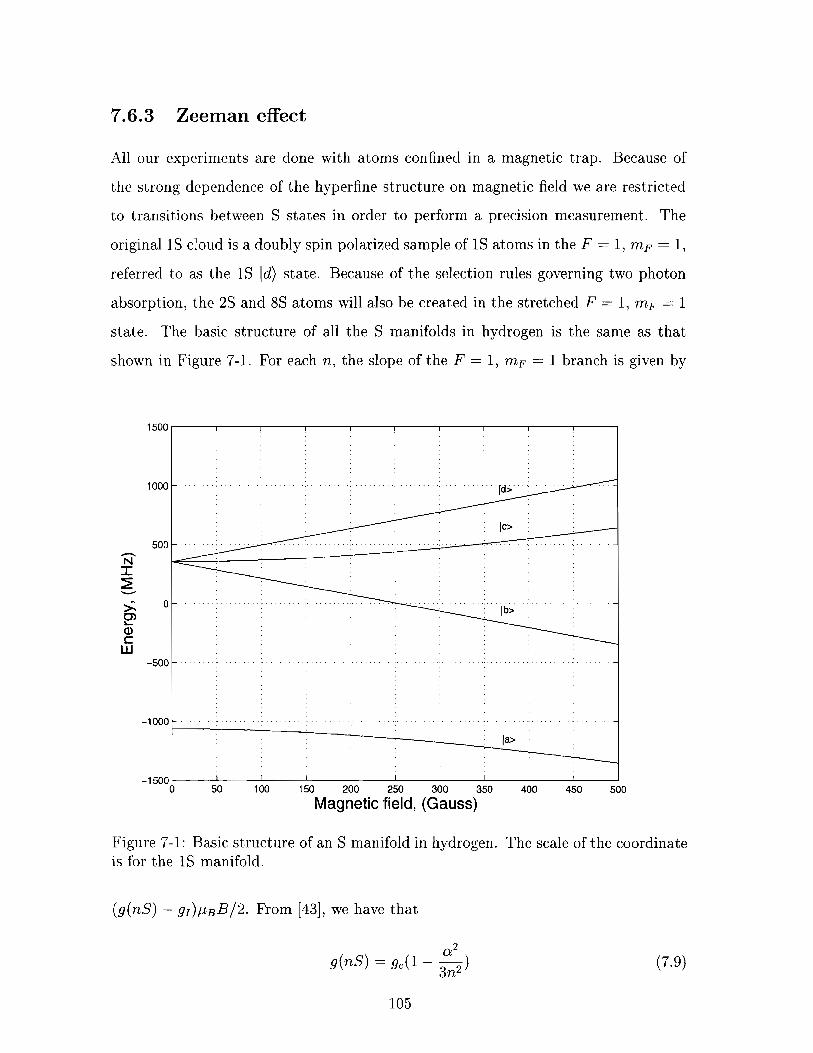
7.6.3 Zeeman effect
All our experiments are done with atoms confined in a magnetic trap. Because of
the strong dependence of the hyperfine structure on magnetic field we are restricted
to transitions between S states in order to perform a precision measurement. The
original 1s cloud is a doubly spin polarized sample of 1s atoms in the F = 1, r n ~ = 1,
referred to as the 1s Id) state. Because of the selection rules governing two photon
absorption, the 2s and 8 s atoms will also be created in the stretched F = 1, r n ~ = 1
st'ate. The basic structure of all the S manifolds in hydrogen is the same as that
shown in Figure 7-1. For each n, the slope of the F = 1, r n ~ = 1 branch is given by
Figure 7-1: Basic structure of an S manifold in hydrogen. The scale of the coordinate is for the IS manifold.
(g(nS) - g1)p~B/2 . From [43], we have that

to order a2. The range in energies for the n to m splitting for a range in magnetic
fields of AB is then given by
Using AB = kBT/pB we have
for the spread of frequencies in a cloud of temperature T. For a 100pK cloud this
gives
While the spread in frequencies of 28 Hz for the IS-2s line seems significant compared
to the natural line width, it is small compared to the width of the expected signal
which will have contributions from time-of-flight broadening and the finite UV laser
linewidth. The 9Hz spread in frequencies for 2s-8s is negligible compared to the
natural linewidth of 72 kHz @ 778 nm and our other expected errors.
7.6.4 Second order Doppler effect
Both the IS-2s and 2s-8s signals that we wish to study arise from Doppler-free
two photon absorption, i.e. the atom absorbs one photon from each of two counter-
propagating beams. Hence, for perfectly aligned beams, there are no effects due to
the first order Doppler shift . The second order Doppler shift is given by
In the simplistic approximation where all the atoms contribute equally to the signal,
the shift can be calculated by substituting the mean-square velocity v =
into Eqn 7.11. At a temperature of 100 pK, the hydrogen atoms are moving at a
velocity of around 1.6 m/s. This gives rise to a fractional frequency shift of 1.4 x 10-l7
or a shift at 243nm of 0.02 Hz (IS-2s) and at 778 nm of 0.005 Hz (2s-8s). Due to the
spread in velocities, there will be a broadening of the same order of magnitude. Both
shift and broadening are clearly negligible in our trap.
By comparison, the atoms in hydrogen beam experiments are moving at around
4000 m/s which, with a more detailed analysis, gives a second order Doppler shift of
40 kHz and a similar broadening. This is calculated to add around a 2 kHz uncertainty
to the extracted frequency 1281.
7.6.5 Cold collision shift
In experiments with trapped hydrogen using the 1s-2s transition, we have observed
a frequency shift which is linearly dependent on the sample density [3,44]. This cold
collision frequency shift arises when the energy levels of an atom are shifted due to
int,eractions with neighboring atoms. It is clearly visible for densities above 1013 cm-3
in the Doppler-free 1s-2s spectrum2.
A theory for the shift has been developed in the low temperature regime to explain
the observations in cryogenic hydrogen masers [45] and more recently in laser cooled
atomic fountains [46-481. The calculations assume a homogeneous sample and a
ho~nogeneous excitation and result in a collision shift due to elastic collisions for a
% broadening is predicted to accompany the shift [3]. However the importance of the broadening decreases with decreasing temperature and at 100pK should be small compared to the linewidth due to other effects. There has so far been no experimental observation of the broadening in trapped hydrogen.
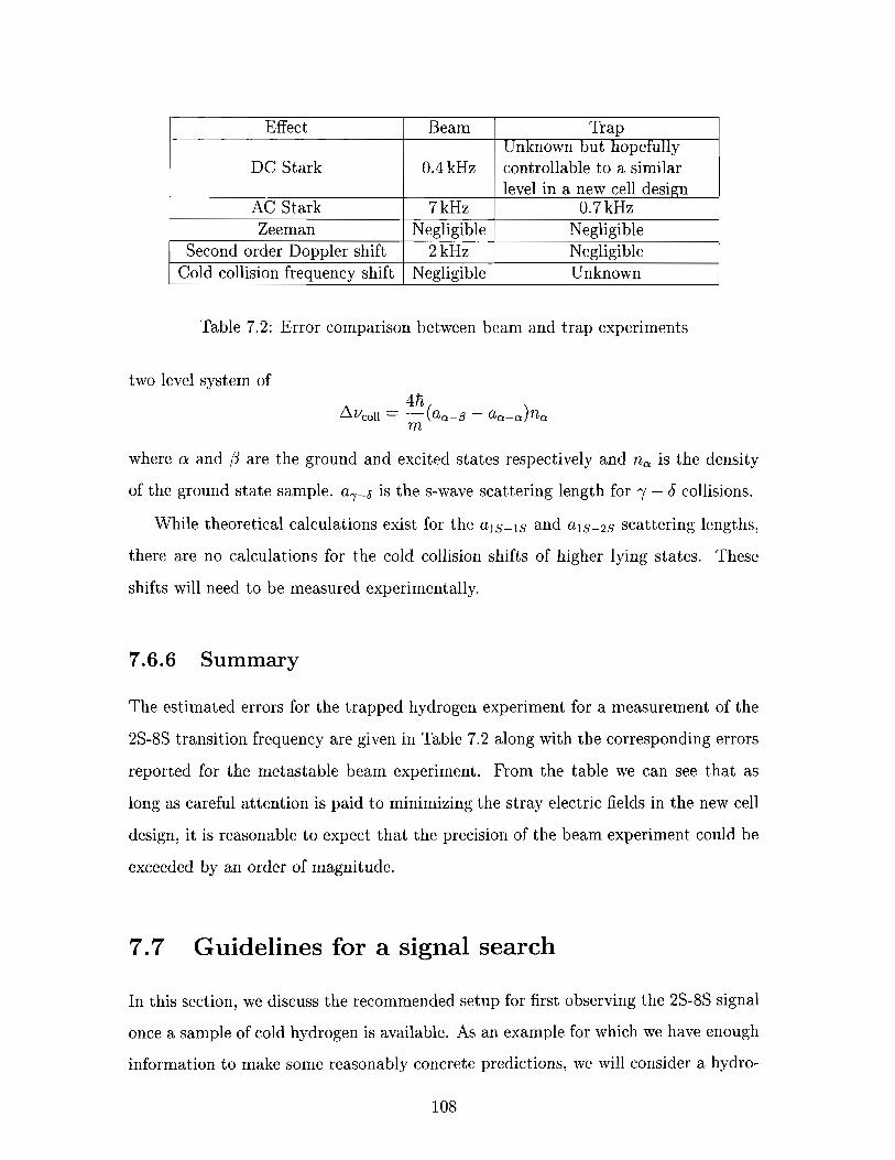
Table 7.2: Error comparison between beam and trap experiments
Effect
DC Stark
AC Stark Zeeman
Second order Doppler shift Cold collision frequency shift
two level system of
where a and p are the ground and excited states respectively and n, is the density
of the ground state sample. a,-6 is the s-wave scattering length for y - 6 collisions.
While theoretical calculations exist for the a1s-1~ and als-2s scattering lengths,
there are no calculations for the cold collision shifts of higher lying states. These
shifts will need to be measured experimentally.
Beam
0.4 kHz
7 kHz Negligible
2 kHz Negligible
7.6.6 Summary
Trap Unknown but hopefully controllable to a similar level in a new cell design
0.7 kHz Negligible Negligible Unknown
The estimated errors for the trapped hydrogen experiment for a measurement of the
2s-8s transition frequency are given in Table 7.2 along with the corresponding errors
reported for the metastable beam experiment. From the table we can see that as
long as careful attention is paid to minimizing the stray electric fields in the new cell
design, it is reasonable to expect that the precision of the beam experiment could be
exceeded by an order of magnitude.
7.7 Guidelines for a signal search
In this section, we discuss the recommended setup for first observing the 2s-8s signal
once a sample of cold hydrogen is available. As an example for which we have enough
information to make some reasonably concrete predictions, we will consider a hydro-

gen sample in Trap W (illustrated in Figure 7-2) as defined by David Landhuis 141.
For a temperature of 87pK, this trap has a thermal radius a,-, = I l l pm in the
Magnetic Potential for Trap W 800
4'1.5 E Depth: 0.826 mK: Y
7, = 9.49 . - Q N - 0 263 2 1 - -Te_mperature; 0.087 mK . . . . IS. ..IS 7 . : . . . . . . . . . . . . . .
+ C a, +-r
0 I 1 I 1
Figure 7-2: Potential and characteristics of the I S sample in Trap W. From Ref. 141.
radial dimension and a, = 38 mm in the axial dimension. The initial 1s density is
no,ls = 6.5 x loL3 ~ m - ~ and the total number of 1s atoms is Nls = 1.3 x 10". For a
UV laser power of around lOmW, a beam waist at the cloud of wo = 21 pm, and a
UV pulse length of 2 ms, we can estimate that around 1 x lo8 metastable atoms are
produced in a single UV shot with the laser on resonance. The metastable decay rate
in the trap was measured to be around 25s-' 141.
For this trap, elastic IS-2s collisions are such that the mean free path for a 2s atom
is on the order of the radial thermal radius. Hence a radial equilibrium distribution is
rapidly established. Axial motion is better described by diffusion and for these trap
parameters, the net distance traveled in 20 ms is only around 2 mm [4]. The initial
distribution of metastable atoms in z was simulated by Lorenz Willmann and David

Landhuis for the given UV laser parameters. The majority of the metastables are
created within 10 mm of the laser focus.
Along with knowledge of the metastable distribution, we need to know the inten-
sity dependent two-photon excitation rate for a single atom. From [49] we have that
the two photon transition rate between the two states lg) and (e) due to two-photon
excitation is
where n, is the number of photons per unit volume in each counter-propagating
wave, re is the natural line width of the excited state, w is the laser frequency, ?is
the polarization of the light, ;is the electric dipole moment operator and the sum is
over all possible intermediate states including the continuum. We can now define
and rewrite Eqn 7.12 as
where a0 is the Bohr radius, a is the fine structure constant, m is the mass of the
electron, I = n,hc is the power density and (elQtplg) is in atomic units. In our
experiment, the incident light has linear polarization and (e 1 Qtp 1 g) has been calculated
to be -14.921 [49].
On resonance we have
If we take re as being close to the natural linewidth of 2 7 ~ x 144 kHz @ 389 nm, this
corresponds to a saturation intensity of I,,, = 5.2 x lo8 W/m2.
With knowledge of the metastable distribution and the single atom, two-photon
transition ratte as a function of intensity, we can now investigate the depletion of the
metastable cloud by spectroscopy of the 2s-8s state. A Monte Carlo simulation was
constructed that propagated atoms with randomly chosen initial conditions within a
two-dimensional harmonic potential. In z, the atoms are approximated as stationary
as discussed earlier. A harmonic potential is a reasonable approximation for our
magnetic trap at low temperature. These atoms interacted with a laser beam with a
Gaussian TEMOO intensity distribution.
Using the trap parameters discussed previously and a total diode laser power of
70 mW, we carried out a Monte Carlo simulation of the metastable depletion for a
range of interaction times. The diode laser beam waist used was wo = 50pm. This
gives a corresponding Rayleigh length of zo = 10 mm which enables us to neglect the
intensity variation in z relative to our metastable sample. The simulation does not
take into account elastic collisions which will change the orbits of atoms in the x-y
plane. These collisions will by definition not change the thermal distribution. The
2s-8s laser beam does change the relative population of orbits, however, because it
preferentially removes atoms in orbits in regions of high intensity. Collisions would
therefore serve to re-populate the orbits with trajectories close to the trap center
which are depleted by the laser beam. Hence neglecting collisions leads to a low
estimate of the total depletion.
The result,~ of the Monte Carlo simulation are shown in Figure 7-3. Figure 7-4
shows the signal-to-noise expected for a single scan across the 2s-8s line if the data is
shot noise limited. The signal to noise is maximized for an laser pulse time of 30 ms
which results in a depletion of around 35%. This should be easily visible with our
current detection system.
We wish to emphasize that these trap and laser parameters are those suggested
for a signal search, not for a precision measurement. The cold collision shift of
3The saturation intensity Isat = hw~I'/12rc2, where I' is the natural lifetime and wo the resonant frequency, is the intensity a t which the photon scattering rate approaches one scattered photon per natural lifetime r
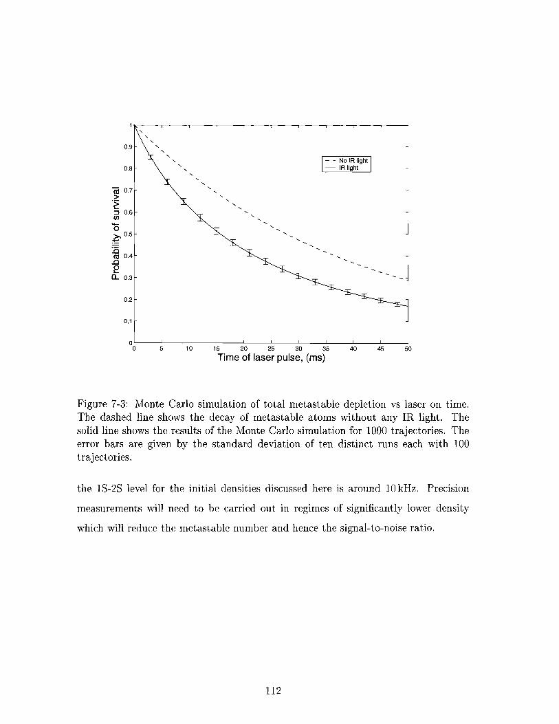
01 I I I I I I I I I 1
0 5 10 15 20 25 30 35 40 45 50
Time of laser pulse, (ms)
Figure 7-3: Monte Carlo simulation of total metastable depletion vs laser on time. The dashed line shows the decay of metastable atoms without any IR light. The solid line shows the results of the Monte Carlo simulation for 1000 trajectories. The error bars are given by the standard deviation of ten distinct runs each with 100 trajectories.
the 1s-2s level for the initial densities discussed here is around 10 kHz. Precision
measurements will need to be carried out in regimes of significantly lower density
which will reduce the metastable number and hence the signal-to-noise ratio.
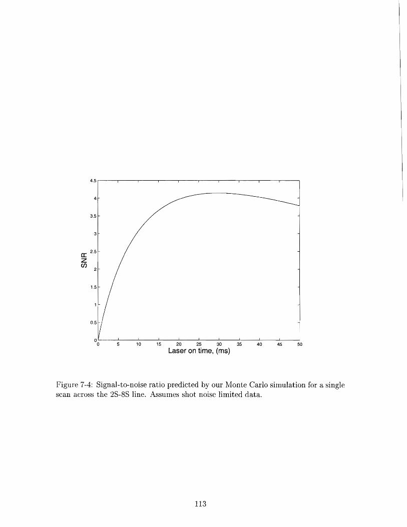
4.5 -- I I I I I I I I I
4 -.
3.5 -.
3 -
IT 2.5 -
z cn
2 -
1.5 -
I I I I
0 I
5 I I I
10 15 20 25 30 35 40 45 50
Laser on time, (ms)
Figure 7-4: Signal-to-noise ratio predicted by our Monte Carlo simulation for a single scan across the 2s-8s line. Assumes shot noise limited data.


Chapter 8
Laser System for 2S-8s two-photon
spectroscopy
This chapter discusses the technical aspects of the 778nm diode laser systems built
to perform 2S-8S spectroscopy.
8.1 Laser overview for 2S-8s measurement
There are three primary requirements for the laser system a t 778nm: accurate fre-
quency referencing, narrow linewidth and high power. In order to make a precision
frequency measurement, we need to be able to reference the frequency of the spec-
trascopy diode laser to the frequency of the 1S-2s transition. This is achieved by
locking the diode to a single mode of a mode-locked femtosecond (fs) comb which in
turn is stabilized to the dye laser that produces the UV light for pumping 1S-2s. The
construction and operation of the femtosecond comb is described in the thesis of Lia
Matos [32]. The laser layout designed to provide sufficient power and tunability to
make a frequency measurement is shown in Figure 8-1. The diode lasers are tuned to
approximately the right frequency using a wavemeter. The iodine laser then gives an
absolute frequency reference to within a few tens of MHz. This allows us to unam-
biguously identify the nearest comb mode (the spacing of modes in the current version
of the comb is 190 MHz). The spectroscopy laser (master laser in Figure 8-1) is then

Menlo Systems I - - - - - - -
I
atoms
I 486 nm dye laser: - -) master frequency reference
locked to 1s-2s transition
Femtosecond 1- - +
comb
to wavemeter
to wavemeter Fiber coupler
to wavemeter
1 Optical beatnote fiber coupled to
(injection locked)
Fiber coupler1
- - - - - - - A -
toatoms
Figure 8-1: Laser layout for 2s-8s frequency measurement. x2 denotes a frequency doubling stage. Approximate power requirements are given where appropriate. APD stands for avalanche photodiode. The dashed lines indicate feedback paths for stabi- lization.
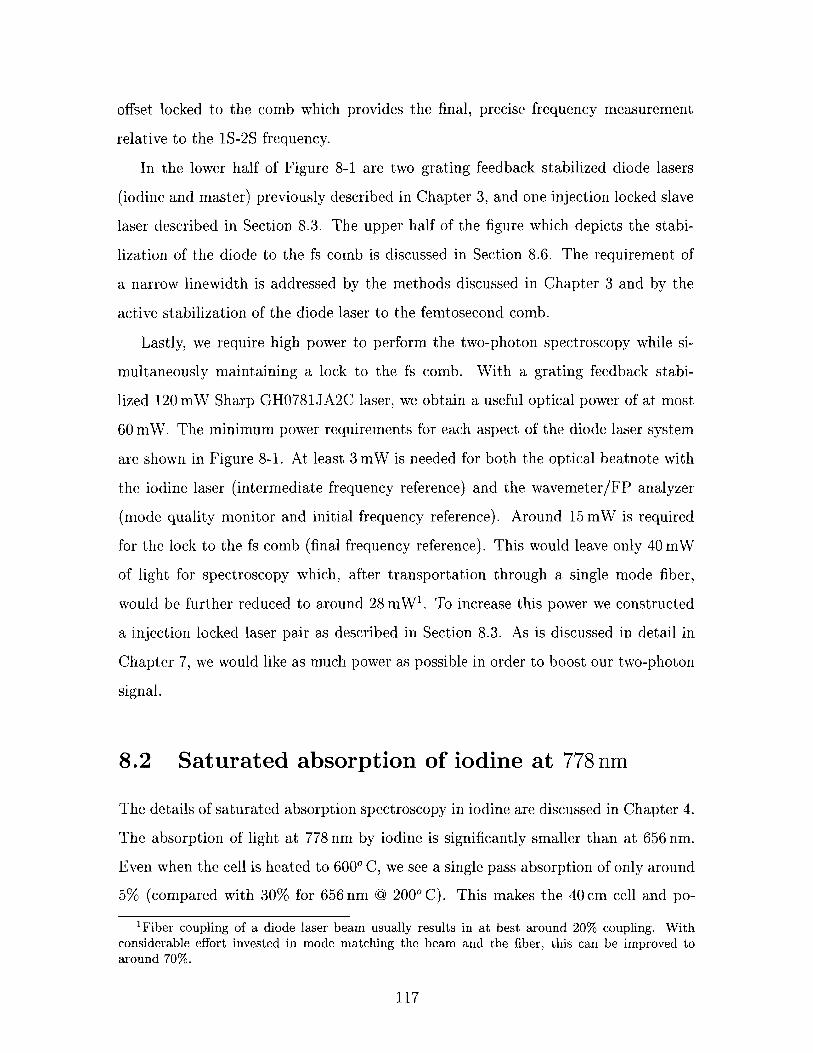
offset locked to the comb which provides the final, precise frequency measurement
relative to the 1s-2s frequency.
In the lower half of Figure 8-1 are two grating feedback stabilized diode lasers
(iodine and master) previously described in Chapter 3, and one injection locked slave
laser described in Section 8.3. The upper half of the figure which depicts the stabi-
lization of the diode to the fs comb is discussed in Section 8.6. The requirement of
a narrow linewidth is addressed by the methods discussed in Chapter 3 and by the
active stabilization of the diode laser to the femtosecond comb.
Lastly, we require high power to perform the two-photon spectroscopy while si-
multaneously maintaining a lock to the fs comb. With a grating feedback stabi-
lized 120 mW Sharp GH0781JA2C laser, we obtain a useful optical power of at most
60 mW. The minimum power requirements for each aspect of the diode laser system
are shown in Figure 8-1. At least 3 mW is needed for both the optical beatnote with
the iodine laser (intermediate frequency reference) and the wavemeter/FP analyzer
(mode quality monitor and initial frequency reference). Around 15 mW is required
for the lock to the fs comb (final frequency reference). This would leave only 40 mW
of light for spectroscopy which, after transportation through a single mode fiber,
would be furt,her reduced to around 28 mW1. To increase this power we constructed
a injection locked laser pair as described in Section 8.3. As is discussed in detail in
Chapter 7, we would like as much power as possible in order to boost our two-photon
signal.
8.2 Saturated absorption of iodine at 778 nm
The details of saturated absorption spectroscopy in iodine are discussed in Chapter 4.
The absorption of light a t 778 nm by iodine is significantly smaller than at 656 nm.
Even when the cell is heated to 600' C, we see a single pass absorption of only around
5% (compared with 30% for 656nm @ 200°C). This makes the 40cm cell and po-
'Fiber coupling of a diode laser beam usually results in a t best around 20% coupling. With considerable effort invested in mode matching the beam and the fiber, this can be improved to around 70%.

larization optics, which allow maximum pump and probe beam overlap, a necessity
rather than a luxury. Figure 8-2 and 8-3 show the theoretical and experimental iodine
spectra in the vicinity of the 2s-8s transition frequency. In wavenumbers, half the
transition frequency from 2s to 8 s is 12853.05 cm-l, indicated on Figure 8-3 by the
dashed vertical line.
Iodine a t 12853 cm-'
calculated vibrational spectrum [ c m - I I
Figure 8-2: Iodine spectrum in the 778 nm region calculated using IodineSpec. The zero on the ordinate axis corresponds to 12853 cm-'. The coordinate axis shows the relative intensity of the various lines. Courtesy of L Willmann, Kernfysisch Versneller Instituut .

Figure 8-3: Experimental iodine spectrum in the 778nm region. The extent of the x axis in wavenumber is approximately 0.06 cm-' by comparison with the calculated spectrum. The dashed line indicates 12853.05 cm-', half the transition frequency from 2 s to 28. The absolute voltage scale for the y axis depends on laser power, alignment, modulation depth, lock-in settings, etc.

8.3 Injection locking
As discussed in Section 8.1, a single grating feedback stabilized diode cannot provide
enough power for both stabilization and spectroscopy. To address this problem, we
use optical injection locking. Diode lasers are extremely sensitive to optical feedback
from any stray light that is coupled back into the laser cavity. In most situations this
is a experimental nuisance, necessitating careful optical design and an expensive and
lossy Faraday isolator to eliminate. However the property can be exploited in a very
useful manner, namely the injection locking of one diode (usually referred to as the
slave laser (SL)) by the deliberate insertion of a small amount of seed light from a
master laser (ML). In this manner the frequency, linewidth and mode quality of one
laser can be transferred to another.
For the 778 nm system, the master laser is a grating feedback stabilized 120 mW
Sharp GH0781JA2C laser. With a gold coated, 1800 l/mm grating blazed for 500 nm [ll]
we achieve a maximum useful output power (light after the Faraday isolator) of around
60 mW. Some 5 mW of this light is split off to injection lock another 120 mW Sharp.
The optical setup for injection locking is illustrated in Figure 8-4. Note that all the
rotations discussed are from the perspective of an observer standing beside the slave
laser, not an observer traveling with the light beams.
The incoming ML light is vertically polarized and is reflected by polarizing beam
splitter 'A' into the Faraday rotator 2. The light is rotated 45" counterclockwise and
exits polarizer 'B' which is orientated to pass light polarized 45" counterclockwise of
vertical. It then passes through a half wave plate which imparts another counter-
clockwise 45" twist resulting in horizontally polarized light. The typical ML power
reaching the SL is 1 - 2 mW. It is possible to injection lock a laser with far less light
than this (say a few tens of /IW). However this makes the alignment significantly
harder and with the current setup we are not so heavily power restricted to make the
added complications of optimized injection locking worthwhile.
2~a raday rotator vs Faraday isolator. The convention we have adopted is that an isolator is a rotator plus two polarizing beam splitters. The Optics for Research isolators come with detachable polarizers. For injection locking, one polarizer is removed and replaced with a free standing polarizing beam splitter cube to simplify the optical alignment.

Injection locked output beam from slave laser
Polarizing beam splitter
Seed light from master laser
IO-05-0778-HP
Polarizing beam splitter -attached to rotator
Figure 8-4: Optiical setup for injection locking. ML stands for master laser and SL stands for slave laser. $ indicates vertical polarization, tt indicates horizontal polarization.

The SL light is horizontally polarized (along the long axis of the elliptical output
beam profile as is typical for diode lasers). Passing through the half wave plate, it
is rotated 45" clockwise which aligns it with the transmission axis of polarizer 'B'.
It passes through the Faraday rotator, receiving a 45" rotation counterclockwise and
exits the rotator horizontally polarized. This polarization is transmitted by the free
standing polarizing beam splitter cube 'A'.
To facilitate injection locking at high currents, the slave laser is temperature tuned
so that its free running wavelength coarsely overlaps that of the master laser. The
actual temperature used varies from diode to diode but is typically around 5" C below
room temperature. Fine adjustment of the pointing of the seeding light is then usually
sufficient to achieve smooth injection locking over GHz scan ranges. With the current
setup, we have achieved usable output powers from the injection locked laser as high
as 100 mW. This is about 85% of the available diode power as opposed to -- 50%
from a grating stabilized laser. Because the SL light is an exact replica of the ML
light, the injection lock has almost tripled the available output power of the master
laser.
Injection locking is illustrated in Figure 8-5. Each of the three panels a), b) and c)
show a 350 MHz frequency sweep of the scanning F P analyzer across a laser mode.
In a), there is only the free running SL. In b), the seed light from the ML is just
starting to see gain in the SL resonator. Note that the power in the free running laser
mode is already reduced. In c), the SL light has completely won the mode competition
and the free running laser mode has vanished. Note that the seed light, which comes
from a grating stabilized laser, results in a narrower mode. The apparent full width
at half maximum (FWHM) of the injection locked mode is the approximately 10 MHz
expected from the F P analyzer (the laser is much narrower (see Section 8.4)). The
apparent width of the free running laser is 18 MHz. De-convolving this from the
-- 10 MHz cavity width suggests a free running laser linewidth of around 15 MHz.
Referring back to Figure 8-1, we can see that with injection locking, the power
available for spectroscopy has increased to -- 70% x 100 mW = 70 mW. As the ex-
pected two-photon signal rate scales as 12, this 2.5 times gain in laser power translates
Figure 8-5: Injection locking of a 778nm diode. a) shows the free running laser. b) shows the situation of partial injection locking where the seed beam is just starting to see gain in the slave laser. c) shows full injection locking where all the power of the slave laser has been transferred to the injected seed mode. All traces are broadened by the - 10 MHz line width of the Fabry-Perot analyzer used to measure the spectra.
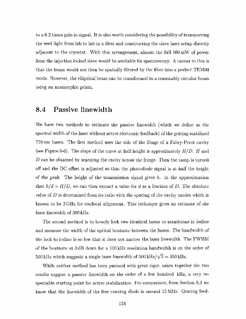
to a 6.2 times gain in signal. It is also worth considering the possibility of transporting
the seed light from lab to lab in a fiber and constructing the slave laser setup directly
adjacent to the cryostat. With this arrangement, almost the full 100mW of power
from the injection locked slave would be available for spectroscopy. A caveat to this is
that the beam would not then be spatially filtered by the fiber into a perfect TEMOO
mode. However, the elliptical beam can be transformed to a reasonably circular beam
using an anamorphic prism.
8.4 Passive linewidth
We have two methods to estimate the passive linewidth (which we define as the
spectral width of the laser without active electronic feedback) of the grating stabilized
778nm lasers. The first method uses the side of the fringe of a Fabry-Perot cavity
(see Figure 8-6). The slope of the curve at half height is approximately HID. H and
D can be obtained by scanning the cavity across the fringe. Then the ramp is turned
off and the DC offset is adjusted so that the photodiode signal is at half the height
of the peak. The height of the transmission signal gives h. In the approximation
that h ld = H I D , we can then extract a value for d as a fraction of D. The absolute
value of D is determined from its ratio with the spacing of the cavity modes which is
known to be 3 GHz for confocal alignment. This technique gives an estimate of the
laser linewidth of 300 kHz.
The second method is to loosely lock two identical lasers to transitions in iodine
and measure the width of the optical beatnote between the lasers. The bandwidth of
the lock to iodine is so low that it does not narrow the laser linewidth. The FWHM
of the beatnote at 3 dB down for a 100 kHz resolution bandwidth is on the order of
500 kHz which suggests a single laser linewidth of 500 k ~ z / f i = 350 kHz.
While neither method has been pursued with great rigor, taken together the two
results suggest a passive linewidth on the order of a few hundred kHz, a very re-
spectable starting point for active stabilization. For comparison, from Section 8.3 we
know that the linewidth of the free running diode is around 15 MHz. Grating feed-
Figure 8-6: Illustration of a linewidth measurement using a Fabry-Perot cavity fringe. H is the amplitude of the cavity fringe. D is the full width half maximum of the fringe. h is the amplitude of the transmission signal when the laser is fixed at the frequency corresponding to half the amplitude H. d corresponds to the width of the laser

back stabilization coupled with good passive design has reduced the laser linewidth
by more than an order of magnitude.
8.5 Phase lock between two diodes
As a testing ground for phase locking the diode to the femtosecond comb, we initially
developed the required phase detector and loop filter electronics by phase locking two
778 nm grating stabilized diode lasers together at some offset frequency determined by
a local oscillator. A phase-locked loop (PLL) is an electronic circuit that controls an
oscillator (in this case one laser of two which form a radio frequency beatnote) so that
it maintains a constant phase angle relative to a reference signal (a local oscillator).
A block diagram of our PLL is shown in Figure 8-7. An optical beatnote is formed
Local ................. oscillator I phase ~..- Beatnote .................
4 7 detector I
#2 Fast
Phase ................ error
i"-pl filter
photodiode
Figure 8-7: Block diagram of phase locked loop
by overlapping light from the two lasers via an optical fiber onto a fast photodiode
(Thorlabs 2 GHz SV2-FC). The beatnote signal to noise can be up to -- 50 dB. The
beatnote is amplified and fed into a digital phase detector (for details of the digital

phase detection see the thesis of Lia Matos [32]). The phase detector gives a phase
error signal derived from the comparison of the beatnote to the local oscillator (an
HP 8657B). The output of the phase detector then goes to the loop filter shown in
Figure 8-8. Th.e basic design is from a JILA circuit, adapted by Lia Matos. For the
diodes we use only the invertible fast path, feeding directly back to the laser diode.
The first stage is a simple non-inverting amplifier with a single pole. The filter corner
frequency is determined by a selectable R and C. We typically use an R of 22 kR and
a C of 1000 pF. The second stage is an inverting amplifier with two poles and a zero.
We have had good success with R19 20 kR, R34 I kR, R37 200 kR potentiometer,
C144 1 p F and C112 open. (Component numbering refers to circuit numbering in
Figure 8-8.)
We have picked up some tips specifically for locking laser diodes from the group
of Leo Hollberg at NIST[12]. Direct feedback to the laser diode, after the current
controller, allows the highest loop bandwidth. Coupling to the diode is accomplished
with the circuit shown in Figure 8-9. We currently use R1 of 10 kR, R2 of 39 0, C
of 47 pF and L of 10 pH. The inductor decouples the feedback from the laser current
source. The paxallel capacitance C is used to introduce phase-lead. According to
[12], most laser diodes have a phase response that rolls off sharply near 1 MHz and
some phase-lead adjustments are required to compensate for this in order to maximize
the filter bandwidth. The resistor R2 in series with C is to limit the high frequency
gain above 30 MHz, preventing parasitic loop oscillations a t very high frequencies.
Although we do not have the facilities to probe the open loop gain of our system and
the response of each component in detail in order to optimize the circuit entirely, we
have seen an improvement in the lock bandwidth when the phase-lead components
are included.
A typical beatnote between two diodes when the phase lock is switched on is
shown in Figures 8-10 and 8-11. Figure 8-10 has a large frequency span and
clearly shows that the bandwidth of the electronic feedback is around 170 kHz. The
width of the central spike simply reflects the resolution bandwidth of the spectrum
analyzer. Figure 8-11 has a 50 Hz frequency span and a 1 Hz resolution bandwidth,
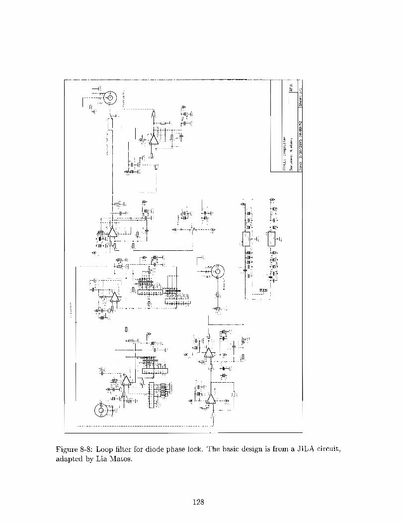
Figure 8-8: Loop filter for diode phase lock. The basic design is from a JILA circuit, adapted by Lia Matos.

Laser current source
L
In from loop filter
Laser
- Figure 8-9: Circuit for feeding back the output of the loop filter directly to the laser diode. Typica,l component values are given in the text.
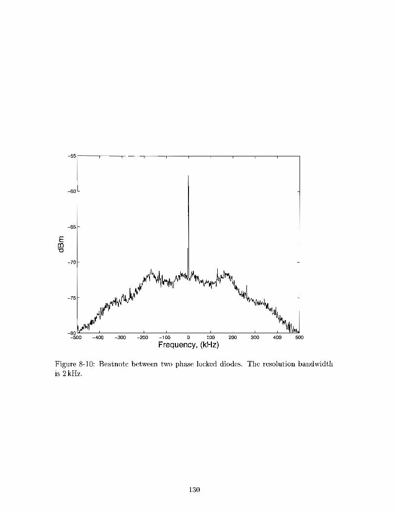
Figure 8-10: Beatnote between two phase locked diodes. The resolution bandwidth is 2 kHz.
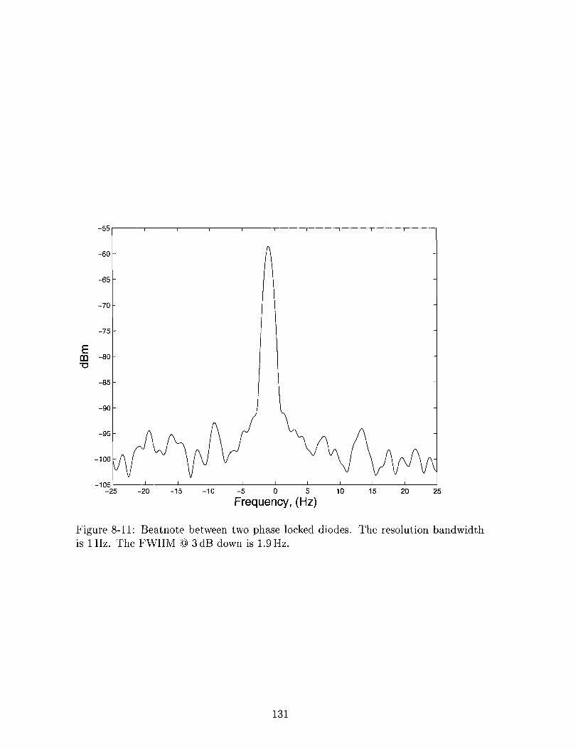
Figure 8-1 1 : Beatnote between two phase locked diodes. The resolution bandwidth is 1 Hz. The FWHM @ 3 dB down is 1.9 Hz.
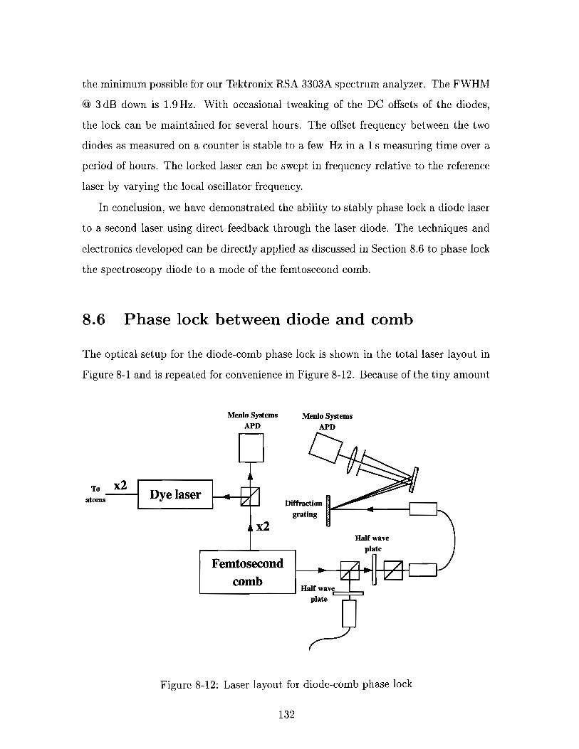
the minimum possible for our Tektronix RSA 3303A spectrum analyzer. The FWHM
@ 3dB down is 1.9Hz. With occasional tweaking of the DC offsets of the diodes,
the lock can be maintained for several hours. The offset frequency between the two
diodes as measured on a counter is stable to a few Hz in a 1 s measuring time over a
period of hours. The locked laser can be swept in frequency relative to the reference
laser by varying the local oscillator frequency.
In conclusion, we have demonstrated the ability to stably phase lock a diode laser
to a second laser using direct feedback through the laser diode. The techniques and
electronics developed can be directly applied as discussed in Section 8.6 to phase lock
the spectroscopy diode to a mode of the femtosecond comb.
8.6 Phase lock between diode and comb
The optical setup for the diode-comb phase lock is shown in the total laser layout in
Figure 8-1 and is repeated for convenience in Figure 8-12. Because of the tiny amount
Menlo Systems Menlo Systems APD APD
I Half wave I
A
I plate I Femtosecond 1 comb 1
, '' Half wave plate -
-
To x2 atoms
Figure 8-12: Laser layout for diode-comb phase lock
4 Dye laser ,/
of light in a single comb mode (- 50 nW), observing reasonable signal to noise on the
comb-diode beatnote is a significant technical challenge. The half wave plate directly
after the out.put of the fiber allows smooth adjustment of the power that is sent into
the beatnote from the diode. The beam combiner is a polarizing beam splitter which
combines vertically polarized light from the diode with horizontally polarized light
from the comb. The second half wave plate mixes the two polarizations. Depending
on the orientation of the second wave plate, the light transmitted by the second cube,
which is also a polarizing beam splitter, contains a smoothly variable mix of the comb
and diode light. In this way, we obtain complete control over the proportion of diode
to comb light.
This light is then coupled into a single mode fiber. This ensures perfect spatial
overlap of the beams from the two different lasers. The fiber output is directed onto
a diffraction grating (Optometrics [ll], 1200 l/mm, blazed for 750 nm, Catalog #3 -
4175). The comb light, which has a bandwidth of some hundreds of nm is dispersed
by the grating. Because of the perfect spatial overlap of diode and comb light, the
diode laser and the comb mode of the closest frequency will remain overlapped while
the rest of the comb modes spread out and can be spatially filtered. Currently we
have N 130cm between the grating and the detector (a Menlo Systems Avalanche
photodiode [50]). The spatial dispersion of the modes is key to achieving good signal
to noise in the heat note as additional comb modes falling on the detector increase
the noise without contributing to the signal. With the optical setup described, we
have achieved a signal to noise of 30 dB which is sufficient to reliably lock the diode
to the comb. The electronics used are the same as those described in Section 8.5.
The locked diode-comb beatnote is shown in Figures 8-13 and 8-14 and The offset
frequency between the diode and the comb as measured on a counter is stable to a
few Hz in a 1 s measuring time. The duration of the lock is currently limited by
instabilities in the comb [32]. When these are resolved, the laser system will be more
than stable enough to perform our 2S-8s precision measurement.

Figure 8-13: Phase locked beatnote between spectroscopy diode and fs comb. The resolution bandwidth is 2 kHz.

Figure 8-14: Phase locked beatnote between spectroscopy diode the fs comb. The resolution bandwidth is 1 Hz. The FWHM @ 3 dB down is 1.0 Hz.


Chapter 9
Conclusion and Outlook
9.1 Outlook for 2s-3P
The 2s-3P experiments described in Chapter 6 were carried out under considerable
time pressure at the tail end of a cryogenic run. Because of this, the techniques were
not explored in detail or polished in any way. However several points of potential
interest have been identified. In this section we discuss the prospects for 2s-3P
spectroscopy in future trapped hydrogen experiments.
9.1.1 Alignment tool in 2s-8s experiments
As mentioned in Section 6.5, the system for 2s-3P spectroscopy is similar to that
designed and built to perform 2s-8s spectroscopy. From our experience with the IS-
2s signal, we know that alignment will be a critical factor in first observing the weak
and narrow 2s-8S signal. Because the same optics can be used for 656 nm (2s-3P) and
778nm (2s-8s) i3 recommendation for the 2s-8s experiment is first to observe and
optimize depletion of the metastable 2S atoms using 2s-3P light. It is then a simple
matter to couple 778 nm light through the same single mode fiber hence switching to
the 2s-8s wavelength without altering the pointing. Good overlap of the cloud and
the 778 nm light is then assured even before a signal is observed.

9.1.2 Optical quench
The 2s atoms excited by UV spectroscopy are metastable, with observed lifetimes of
up to 80 ms in our current cell design. In order to observe good signal to noise when
counting the Lyman-a decay photons on a MCP, we need a way to force the decay
to occur in a much shorter time window, in other words a method to 'quench' the 2s
atoms. An alternative to the electrical quench currently used in our experiments (see
Section 2.3) is an optical quench using a laser tuned to the 2s-3P transition. In this
section, we will discuss the implementation of such an optical quench.
In an electrical quench, we mix the 2s and 2P states via an electric field applied
across the cell. The currently used 10 V/cm results in a 2s lifetime of around 3.6 ps.
This gives a peak MCP signal rate for high UV power of around 10 MHz l . In the
current trapping cell, the quench voltage is applied across the trapping cell by a pair
of opposed electrodes (see Figure 9-1). The electrodes were formed by scratching the
outline of a rectangle through the thin copper skin on the inner surface of the cell.
While the electrodes work well, the construction method has resulted in stray fields
estimated at 40 mV/cm [4]. In our proposed precision measurement in trapped
hydrogen, this level of stray fields would be the limiting error.
If we consider the alternative of an optical quench, creating an effective 2s lifetime
of 3.6 ps with a red beam tuned to 2s-3P would require an intensity of just 0.3% Imt
or around 0.04 mW/cm2. Even filling the cell with a wide beam of this intensity would
introduce no heating problems and the light would not even have to be particularly
close to resonance. The decay from 3P is primarily back to 1s via the emission of
one photon at 103 nm. A major problem with this method is that the transmission of
MgF2 at this wavelength is probably around 20% less than at 121 nm [51] although
this drop in signal may be partially offset by an increased detection efficiency on
the MCP for the shorter wavelength. However, if the primary method of detection
is 2s-3P absorption, then a reduction in the MCP signal is not important. In the
design of a new cell for precision spectroscopy, the use of an optical quench should
'This is close to the maximum signal rate that can be observed with the current plates. Higher count rates result in missed counts because of the finite dead time of the MCP.

@ Atoms
Figure 9-1: Cross section of the trapping cell showing the quench electrodes (adapted from [dl)

be considered as it eliminates the need for quench electrodes and hence allow the
construction of a cell with extremely low stray electric fields.
9.1.3 Detection method for metastables
As discussed in detail in Section 6.6, absorption of light on the 2s-3P transition offers
an alternative method for metastable detection with the potential for much higher
signal to noise than the currently used MCP method. Because optical access to the
atomic cloud will be from the bottom rather than from the top of the fridge, it should
be possible to have the last room temperature accessible folding mirror for beam
steering only 30 cm from the atoms instead of the current 270 cm. This makes it
entirely feasible to expect near perfect overlap of the atomic cloud with a laser beam
of comparable diameter. In this situation, it should be possible to approach the shot
noise limit for 2s-3P absorption spectroscopy.
9.2 Outlook for 2s-8s and precision spectroscopy
While the primary goal of performing a high precision measurement of the 2s-8s
frequency in cold trapped hydrogen was not realized, the laser systems for this mea-
surement now sit poised for action as soon as sufficiently cold hydrogen samples are
obtained in the new apparatus. As this thesis has demonstrated, with a new cell
designed specifically for precision spectroscopy, the Ultracold Hydrogen Group has
every chance of performing a new measurement of the 2s-8s transition frequency
with an accuracy ten times higher than the current best measurement. All of the
tricks and techniques for manipulating diode lasers acquired during the course of this
thesis research can also be extended to additional laser systems allowing precision
measurements of further 2s-nS transition frequencies.

Bibliography
[I] John S Itigden. Hydrogen: the essential element. Harvard Univeristy Press, 2002.
[2] Dale G. Fried. Bose-Einstein condensation of atomic hydrogen. PhD thesis,
Massachusetts Institute of Technology, 1999.
[3] Thomas Charles Killian. I S - 2 s spectroscopy of trapped hydrogen: The cold colli-
sion frequency shzjl and studies of BEC. PhD thesis, Massachusetts Institute of
Technology, 1999.
[4] David Paul Landhuis. Studies with Ultracold Metastable Hydrogen. PhD thesis,
Harvard University, 2002.
[5] H T C Stoof, J M V A Koelman, and B J Verhaar. Spin-exchange and dipole
relaxation rates in atomic hydrogen: rigorous and simplified calculations. Phys
Rev B, 38(7):4688, 1988.
[6] Julia K. Steinberger. Progress towards high precision measurements o n ultracold
metastable hydrogen and trapping deuterium. PhD thesis, Massachusetts Institute
of Technology, 2004.
[7] Jon Carl Sandberg. Research towards laser spectroscopy of trapped atomic hy-
drogen. PhD thesis, Massachusetts Institute of Technology, 1993.
[8] Stephen C. Moss. Formation and Decay of a Bose-Einstein condensate in atomic
hydrogen. PhD thesis, Massachusetts Institute of Technology, 2002.
[9] Carl E Wieman and Leo Hollberg. Using diode lasers for atomic physics. Review
of Scientific Instruments, 62(1): 1, 1991.
[lo] Thorlabs, http://www.thorlabs.com, AE0203D04 Piezo-electric stack.
[ll] Optometrics LLC, http://www.optometrics.com.
[12] Private communication, Leo Hollberg.
[13] S Gerstenkorn and P Luc. At las d u spectre dabsorpt ion de la molecule diode.
Editions du CNRS : Diffusion, Presses du CNRS, 1978.
[14] Anthony E Siegman. Lasers. University Science Books, 1986.
[15] Paul Horowitz and Winfield Hill. T h e Art of Electronics. Cambridge University
Press, 1980.
[16] Opthos Instruments, http: //www.e-opthos.com.
[17] Omega Engineering, http://www.omega.co, CL3512A Digital thermometer.
[18] Barnstead International, http://www.barnsteadthermolyne.com, HC503X1
quartz insulated heater tape, 115V.
[19] McMaster-Carr. http://www.mcmaster.com, 8 lbs/cu ft, Cat# 93315K61.
1201 McMaster-Carr. http://www.mcmaster .corn, Cat #9364K59.
1221 D J Berkeland, E A Hinds, and M G Boshier. Precise optical measurement of
Lamb shifts in atomic hydrogen. Physical Rev iew Let ters , 75(13) :2470, 1995.
[23] http://www.newfocus.com New Focus. Model 1577, 12-GHz Amplified Free-
Space Photoreceiver.
[24] http://www.thorlabs.com Thorlabs. FS-SN-3224, 630nm single mode fiber. Op-
erating wavelength is typically 50nm below to 200nm above the design wave-
length.
[25] MIT Physics. MIT 8.421 (Atomic and Optical Phyiscs) course notes.
142
[26] Robert decarvalho. Inelastic scattering of magnetically trapped atomic
chromium. PhD thesis, Harvard, 2004.
[27] M Niering, R Holzwarth, J Reichert, P Pokasov, Th Udem, M Weitz, T W
Hansch, P Lemonde, G Santarelli, M Abgrall, P Laurent, C Salomon, and A Cla-
iron. Measurement of the hydrogen 1S-2s transition frequency by phase coherent
comparison with a microwave cesium fountain clock. Physical Review Letters,
84(24) : 5496, 2000.
[28] B de Beauvoir, C Schwob, A Acel, L Jozefowski, L Hilico, F Nez, L Julien,
A Clairon, and F Biraben. Metrology of the hydrogen and deuterium atoms:
Determination of the Rydberg constant and Lamb shifts. European Physical
Journal D, 12:61, 2000.
[29] F Nez, M D Plimmer, S Bourzeix, L Julien, F Biraben, R Felder, 0 Acef, J J
Zondy, P Laurent, A Clarion, M Abed, Y Millerioux, and P Juncar. Precise
frequency measurement of the 2 s - 8S/8D transitions in atomic hydrogen: New
determination of the Rydberg constant. Physical Review Letters, 69(16):2326,
1992.
[30] B de Beauvoir, F Nez, L Julien, B Cagnac, F Biraben, D Touahri, L Hilco,
0 Acef, A Clairon, and J J Zondy. Absolute frequency measurement of the
2 s - 8 S I D transitions in hydrogen and deuterium: New determination of the
Rydberg constant. Physical Review Letters, 78(3):440, 1997.
[31] C Schwob, L Jozefowski, B de Beauvoir, L Hilco, F Nez, L Julien, F Biraben,
0 Acef, a,nd A Clairon. Optical frequency measurement of the 2 s - 1 2 0 transi-
tions in hydrogen and deuterium: Rydberg constant and Lamb shift determina-
tions. Physical Review Letters, 82(25):4960, 1999.
[32] Lia Matos. Title to be determined. PhD thesis, Massachusetts Institute of Tech-
nology, 2005.

[33] W E Lamb and R C Retherford. Fine structure of the hydrogen atom by a
microwave method. Physical Review, 72 (3) :241, 1947.
[34] M Weitz, A Huber, F Schmidt-Kaler, D Leibfried, W Vassen, C Zimmermann,
K Pachucki, and T W Hansch. Precision measurement of the 1s ground-state
Lamb shift in atomic hydrogen and deuterium by frequency comparison. Physical
Review A, 52(4):2664, 1995.
[35] Krzysztof Pachucki. Logarithmic two-loop corrections to the lamb shift in hy-
drogen. Physical Review A, 63:042503, 2001.
[36] K Pachucki, D Leibfried, and T W Hansch. Nuclear-structure correction to the
Lamb shift. Physical Review A, 48(R1), 1993.
[37] L N Hand, D G Miller, and Richard Wilson. Electric and magnetic form factors
of the nucleon. Review of Modern Physics, 35:335, 1963.
[38] G G Simon, Ch Schmitt, F Borkowski, and V H Walther. Absolute electron-
proton cross sections at low momentum transfer measured with a high pressure
gas target system. Nuclear Physics A, 333:381, 1980.
[39] P Mergell, Ulf-G Meibner, and D Drechsel. Dispersion-t heoretical analysis of the
nucleon electromagnetic form factors. Nuclear Physics A, 596:367, 1996.
[40] R Rosenfelder. Coulomb corrections to elastic electron-proton scattering and the
proton charge radius. Physics Letters B, 479:381, 2000.
[41] R Pohl, F Biraben, C A N Conde, C Donche-Gay, T W Hansch, F J Hartmann,
P Hauser, V W Hughes, 0 Huot, P Indelicato, P Knowles, F Kottmann, Y W
Liu, V E Markushin, F Mulhauser, F Nez, C Petitjean, P Rabinowitz, J M F dos
Santos, L A Schaller, H Schneuwly, W Schott, D Taqqu, and J F C A Veloso.
Towards a measurement of the Lamb shift in muonic hydrogen. In The Hydrogen
Atom: Precision Physics of Simple Atomic Systems, Lecture Notes in Physics.
Springer-Verlag, 2001. Contributed paper on CD only.
[42] Savely G Karshenboim. Two-loop logarithmic corrections in the hydrogen lamb
shift. Journal of Physics B: Atomic, Molecular and Optical Physics, 29:L29,
1996.
[43] Hans A Bethe and Edwin E Salpeter. Quantum Mechanics of one- and two-
electron at oms. Springer-Verlag, 1957.
[44] T K Killian, D G Fried, L Willmann, D Landhuis, S C Moss, T J Greytak, and
D Kleppner. Two-photon spectroscopy of trapped atomic hydrogen. Physical
Review Letters, 81:3807, 1998.
[45] B J Verhaar, J M V A Koelman, H T C Stoof, and 0 J Luiten. Hyperfine
contributions to spin-exchange frequency shifts in the hydrogen maser. Physical
Review A, 35:3825, 1987.
[46] E Tiesinga, B J Verhaar, H T C Stoof, and D van Bragt. Spin-exchange frequency
shift in a cesium fountain. Physical Review A, 45:R2671, 1992.
[47] K Gibble and S Chu. Laser-cooled Cs frequency standard and a measurement of
the frequency shift due to ultracold collisions. Physical Review Letters, 70: 1771,
1993.
[48] S Ghezali, Ph Laurent, S N Lea, and A Clarion. An experimental study of
the spin-exchange frequency shift in a laser-cooled cesium fountain frequency
standard. Europhysics Letters, 36(1) :25, 1996.
[49] J C Garreau, M Allegrini, L Julien, and F Biraben. High resolution spectroscopy
of the hydrogen atom. 11. Study of line profiles. Journal of Physics, France,
51:2275, October 1990.
[50] Thorlabs, http://www. thorlabs.com, APD210.
[51]See for example the curves for magnesium fluoride at
http://www.rainbowoptics.com.