lsl. OF TEC 1

(1959) May 27 1997Henry WilMtUam Brdi1

I-S

-A

R

B. ST, Tute Univerety(1959)

SUBMITTED IN PARTIAL FULFILLMENTOF THE REQUIREMNTS FOR TC- s

DEGREES OF MASTER OF WSCIENCE FROM

MIT ES

MASSACHU E TS INSTITUTE OF TECNOOYMay, 1965

IN1 1965

CerStiMed by.o. ... ... - -- , - . .. ,.. ... .. .....................S. T ommiees Soupervisor

Acceptod by ...e a 0 10So, 090 *.... 0. . ..... * 0 00 605 00004

Aox yDepartment Commttee on Graduate Students

ATMOSPHEkIC POLLUTION BY OZONE:ITS EFFECTS AND VARIABILITY

by

Henry William Brandli

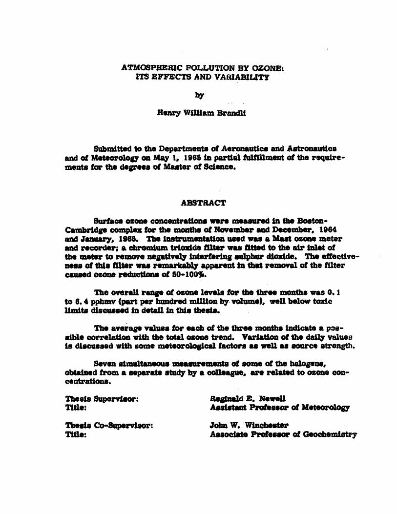
Submittod to the Departments of Aeronautics and Astronauticsand of Meteorology on May 1, 1966 in partial fulfillment of the require-ments for the degrees of Master of Science.

ABSTRACT

Surface ozone concentrations were measured in the BostonCambridge comples for the months of November and December, 1984and January, 1965. The lastrumentation used was a Mast osone meterand recorder; a chromium triide filter was fitted to the air inlet ofthe meter to remove negatively interfering sulphur didaide. The effective-ness of this ilter was remarkably apparent in that removal of the filtercaused ozone reductions of 50-100%.

The overall range of ozone levels for the three months was 0,to 6. 4 pphmv (part per hundred million by volume), weUl below toxiclimits discussed in detail in this thesis.

The average vales for each of the three months indicate a pos-sible correlation with the total ozone trend. Variation of the daily valuesis disussed with some meteorological factors as wel as source strength.

Seven simultaneous measurements of some of the halogens,obtained from a separate study by a colleague, are related to ozone con-centrations.

Thesis Supervisor: Reginald E. NewellTitle: Assistant Professor of Meteorology

Thesis Co-Supervisor: John W. WinchesterTitle: Associate Profesor of Geochemistry

*-3-

TABLE OF CONTENTS

LIST OF FIGURES

FigureFigre

Figure 3.

FigureFigure

Figure 6.

Vertical distibution of osoe (umkehr method)Vertical diatbibution of ozone (rocket and ozone-sande)Isopleths otverage ozone amount (month andlatitude) ...Vertical transport mechanismsMaximum daily values of surface ozone (Boston-Cambridge)Peak ozone values versus beta activity in sur-face air

LIST OF TABLES

Table 1. Surface osone values in Boston-Cambridge com-plex

Table . Effectiveness of Chromium Trioxide FilterTable 3. Stability versus ozons concentrationTable 4. Traffic density versus ozone concentration

I INTRODUCTION

II DESCRIPTION OF OZONE

A. PrpertteeB. Uses

IU TOXICITY

A. Effect on PlantsB. Effect on AnimalsC. Effect on Humans

IV FORMATION AND DISTRIBUTION OF ATMOSBPERIC OZONE

A. Upper AtmosphereB. Transport Properties

6.4

1010

131417

2126

-4-

Table of Contents, cont.

Page

C. Lower Atmosphere 30D. Other possible mechaniams in ozone formation 34

V INSTRUMENTATION

A. Osone measuring devices 3,7B. Disturbing agents in the electrochemical (KI) method

of ozone analysi (use of filter) 41

VI SAMPLING SITE8 4.5

VII DISCUSSION OF RESULTS

A. Osone measurements in Boston-Cambridge complex 4B. Past Measurements 5 1C. Effectiveness of Chromium Trioxide Filter 5 4D. Discussion of results with respect to

1. Past Measurements 5 62. Meteorological Factors 573. Source Strength 81

E. Relationship between ozone and some members ofthe halogen family1. Relation ozone to chlorine '2. Relation of Bromine and Iodine to osone 67

VIII RECOMMENDATIONS 60

IBLIOGRLAPHY 70

APPENDIX AAPPENDIX B 73ACKNOWLEDGEMENTS 70

LIST OF FIGURES

Figure 1. Vertical distribution of ozone (umkehr method)

Figure 2. Vertical distribution of ozone (rocket and ozonesonde)

Figure 3. Isoplethe of average ozone amount (month and latitude)

Figure 4. Vertical transport mechanisms

Figure 5. Maximum daily values of surface ozone (Boston-Cambridge)

Figure 6. Peak ozone values versus beta activity in surface air

LIST OF TABLES

Table 1 Surface ozone values in Boston-Cambridge complex

Table 2. Effectiveness of Chromiunm Trioidde Filter

Table 3, Stability versus ozone concentration

Table 4. Traffic density versus ozone concentration

I INT#ODUCTION

In his State of the Union message to the people of the United

States of America in January of 1965, President Lyndon Baines Johnson

emphasized the need for air pollution studies and control, particularly

in the urban areas of the country, as one of the more important matters

facing the nation.

Ozone is one of the major contaminants that exist n polluted

urban atmospheres and is very harmful to people, plants, and animal

if the concentration to allowed to reach certain levels. On the other

hand, the presence of ozone in the lower stratosphere shields the earth

from the deadly ultra-violet light of the sun.It

Since ozone was discovered in Germany by Schoabeln over one-

hundred years ago, much has been studied and reported about this gas;

however, the majority of the meteorological work done has been with

the use of ozone as a trace substance in the upper atmosphere where

it is produced by photochemical reactions. With the discovery of the

toxic properties of ozone in the last few years, a fact that is still re-

ported incorrectly in some recent literature accounts, a new impetus

in the field of ozone pollution has arisen in measurements and mea-

surement techniques in all levels of the atmosphere particularly in

major urban areas known for pollution problems.

-7-

The concentration of ozone in the upper atmosphere between

20 and 30 kilometers reaches values as high as 10 parts per million

by volume (ppmv) which is a lethal dosage for humans itf exposed to it

for a specified length of time. With the advent of supersonic commer-

cial aircraft flying at levels close to the maxiiuam values of ozone,

these potential toxic effects will present a tremendous problem to the

builders and designers of these planes, a dilemma probably even more

critical than effects of cosmic radiation. Elimination of ozone in these

deadly proportions will undoubtedly be done by the use of filter tech-

niques in the compressor system, possibly of a catalytic nature, as

are used in some high altitude military planes, or of the activated car-

bon type used in the space field. However, the duration of flight in

commercial air travel is in most cases greater than the length of military

or space flights; thus greater dangers are presented due to longer ex-

posure times. The effect of ozone in high-altitude cabins is discussed

in greater detail by Jaffe and Estes (1984).

In the lower levels of the atmosphere, more specifically in

polluted urban areas, it isto important that the levels of ozone concentra-

tion be determined and monitored. Much of this work has been and is

being done in noted smog areas such as Los Angeles and London where

pollution is an immediate problem. But what about other cities and areas

-8-

of this nation and the world where population, industry, and motor

vehicles are increasing at a rapid and somewhat alarming pace? In

this day and age, there seems to be a trend toward moving everything

and everybody into the large city complexes, particularly in the United

States.

The measurements of ozone in the past have been concerned in

large extent with the total amount of ozone in a vertical column of the

atmosphere. But what about sorface concentration measurements or

measurements at a particular level of the atmosphere ? This type of

measurement could be extremely important to the meteorologist or

toxicologist. Recent work by Kawamura (1964) on measurement of

surface ozone in the Tokyo area showed that the concentration of ozone

in the lower troposphere and at the surface varied simultaneously with

total ozone amount. However, in some areas, it is possible that pol-

lution by surface sources is a greater factor in surface ozone concen-

tration than the ozone which is brought down from upper levels by

diffusion, turbulence, and vertical transport. Kawamura's result

could be extremely significant, it valid everywhere, in that former

investigations which used total ozone content could be reviewed some-

what critically perhaps in view of present surface measurements.

It is hoped that new results can be gathered with the use of

-9-

surface ozone measurements such as the variability of ozone in different

air masses, the effects of source strength, and many other comparisons

with regard to the major meteorological parameters. Also comments

about the many reactions, both direct and indirect, on the formation

and destruction of ozone would be an interesting study area to be probed

with better instrumental techniques. Another question to be raised is

"Are the concentrations of surface ozone high enough to create a hazard

to the vital human activity in the area concerned, and it so what solu-

tions should be proposed?"

The author measured surface ozone concentration in the Boston-

Cambridge complex using a portable Mast ozone meter with a filter that

removed the negative interference of sulfur-dioxide. The measurements

were recorded at three different sites n the city complex during the

months of November and December in 1964 and the month of January of

1965.

II DESCRIPTION OF OZONE

A. Properties

Ozone, 03 , is a colorless to blue gas with a pungent odor and

has a gas density of 2. 144g/iter at 0oC. (760mm) which is 50% greater

than oxygen, 02. In high concentrations, ozone has a characteristic

chlorine or sulfur-dioxide like odor, whereas in lower concentrations,

it has a so-called "electrical odor" discernable after a thunderstorm.

Ozone boils at -I t. 9oC (760mm) and melts at -192. 7. It will con-

dense at low temperatures to a blue black liquid. The chemical proper-

ties of ozone are similar to those of oxygen, but ozone is more reactive.

Many substances that do not react at all with oxygen, or only slowly,

react readily with ozone. Silver, for example, which remains bright

and shining for years in ordinary oxygen quickly becomes covered with

a brown film of silver oxide when exposed to air containing a trace of

ozone. Also a stretched rubber band exposeci to the action of ozonized

air snaps in a few seconds showing how rapidly it is oxidised.

13. Uses

Ozone is used industrially in the bleaching of colors and dyes

in textiles and of oils, fate, flour, starch, and sugar in foodstuffs; it

is also used in producing peroxides. The use of ozone has also been

mentioned in the controlling of mold both in fruit produce, particularly

-11-

apples, and also in the dairy industry, namely cheese and cheese products.

Most recently, there has been thought of using high-energy liquid ozone

to replace liquid oygen in rocket fuels, thus. providing a 80% increase

in energy over former conventional liquid fuels, such as hydrogen-oxy-

gen. Recent work done at M. I. T, on the delicate job of controlling and

storing the dangerous and unpredicatable liquid ozone has made this a

leasable proposition.

The last mentioned use of ozone would be a boon In the present

space age; however, there exists the possibility of ozonospheric contam-

ination because the exhaust gases of the rockets. The disruption of the

upper atmosphere could have serious implications on our environment

and would be a very important factor in considering ozone as a fuel for

rockets. This problem of contamination by exotic rocket exhaust gases

on the atmosphere, particularly the upper portions, is getting more

and more acute because of the augmentation in the size of rocket

boosters. The total mass of constituents in the upper atmosphere is

so small, it is conceivable that the exhaust gases will be approaching

these magnitudes. With a possible ftel iUke fluorine which to a

scavenger of electrons, there is a chance of upsetting the Ionosphere,

thus causing severe communication problems as well as other major

disorders. The subject of atmospheric modification by rocket exhausts

-12-

is not discussed in detail here, but the author refers interested persons

to the work being done by the Geophysics Corporation of America (Mill-

man et al8 1962).

A few years ago, ozone was frequently advocated as a means

for removing deadly carbon monoxide gas from garages. The ozone

was to be produced by ozone generators, Fortunatelythis scheme was

found to be too slow to convert carbon monodide to carbon dioxiae. Of

course if the toxic properties of ozone were well known at that time,

the above proposal would have been absurd. The important topic, ozone

toxicity, is discussed in the next section.

-13*

III TOXICITY

A. Effect on plants

In a 1962 report to the Congress of the United States, the Surgeon

General related that plant damage by air pollution cost the nation between

one hundred and fifty and five hundred million dollars annually. One of

the major air pollutants mentioned as a cause of this damage was ozone.

Many observers and investigators in the nineteen forties noticed

smog effects on leaty vegetables and other crops in the Southern Califor-

nia area. A constituent of photochemical smog. ozone was studied with

regard to the plant problem by Haagen-Smit et a (1952). They showed

that the combination of ozone at 28 parts per hundred million by volume

(pphmv) and gasoline vapors at 340 pphmv produced the same plant dam-

age as observed in the area mentioned above.

Richards et al (1958) reported that ozone might be the cause

of stipple disease on grapes in California. Later Reggestad and

Middleton (1959) showed that "weather fleck" disease on tobacco plants

could be produced by exposure to ozone, and that high ozone levels were

correlated with observed fleck reports. In a Connecticut study, Sand

(1959) found that experimental concentrations of ozone greater than 10-

20 pphmv produced this leaf tissue injury called fleck in susceptible

varieties of tobacco. This susceptibility to fleck is partly genetic as

-14-

Was demonstrated by hybridization experiments in the New Haven,

Connecticut station. Sand also mentioned that physical or chemical

measures to close the leaf Stomata, or antioxidant sprays to diminish

the local concentration of ozone reduced fleck injury.

A suggestion by Daines e a (1960) in a preliminary study was

that a disease of spinach may be related to atmospheric ozone concen-

tration.

The effects of ozone are probably produced by its action on the

cell enzymes of the plants discussed. Freebairn (1959) demonstrated

that certain reducing agents such as glutathione and ascorbic acid

tended to hinder the effects of ozone upon certain reducing groups in

vital protein molecules. Further field tests Indicated that the damaging

effects of smog-associated ozone upon plants were reduced by the use

of vitamin C (ascorbic acid) sprays.

B. Effect on animals

Ozone effects on animale have been described by many researchers

in papers for a little over a century. From this work, physiologists and

toxicologists have obtained much needed data in hopes of studying man's

adaptations to ozone.

In an experiment by Diggle and Gage (1955), they found that the

LD5 0 (lethal dosage in fifty per cent of cases observed) for rodents

exposed for a period of four hours was 12 ppm (vol). This is a rather

high concentration of ozone, and it is very unlikely that a concentration

of this magnitude would be found in pOluted air near the ground.

Stokinger (1957) observed that the LD50 for rats and mice also exposed

for 4 hours was 4. 8 - 3. 8 ppm (vol). Mittler 0 (1957) reported using

animals (small) exposed to ozone produced by a corona discharge ozon-

iser that the LDSO in a 3 hour exposure period was 12 ppm (vol) for

rodents in one study and over 20 ppm (vol) in another (1956).

Thorp (1941) suggested that the presence of nitrogen oxides

which could be generated by some osonisers may enhance the toxicity

of ozone. Diggle and Gage in their paper stated that mixtures of ozone

and nitrogen diotide reacted in part to form N20 5 (nitrogen pentoside)

which was about three times as toxic as ozone. Stokinger (1957), how.-

ever, claimed that as a result of many careful studies on test animals

that there are no reasonable grounds for these claims that nitrogen

oxides contribute signifcantly to the toxiity of of oone. In fact, he

reports that the lethal effects of ozone on mice was reduced slightly by

the addition of nitrogen dioxide.

Many conlicting reports of the above nature occur in the

literature. These discrepancies are most likely due to the use of crude

osonisers, unreiable methods of analysis and measurement, and the

-Is-

-16-

presence of organic materials readily attacked by ozone.

The casle of death in the above mentioned studies was due to

acute pulmonary edema and hemorrhage. In other animal studies, it

was found that with repeated exposure to ozone of 1 ppmv (only slightly

higher than reported in some urban areas) 8 hours a day for periods

up to one year, the animals contracted bronchitis, fibrosis, and bron-

chiolitus.

Stokinger et al (1961) demonstrated that several other sub-

stances of oxidative nature including ozone are capable of educing a

comparable acutely tonic response and subsequently causing the de*

velopment of a tolerance toward further intoxication. For example,

pre-exposure to lower levels of ozone seemed to protect animals

from subsequent otherwise lethal dosage;. Also, hydrogen peroxide

(HO, ) administered to mice in repeated dosages of about 20% of the

lethal dose conferred protection on these animals when they were

challenged with acute lethal dosages of ozone. When oone and carbon

dioxide were administered to rodents, it was found that the acute toxicity

of ozone was slightly enhanced. Another interesting discovery was that

oil mists tended.to protect small animals from the ascte effects of ozone.

This protection was only afforded if the animals were exposed to the

mist before comlng in contact with the ozone. If the expoasre to ozone

and mist was atmultaneous, toxhe ticity was slightly intensified. White

mineral oil gave greater protection than motor oil. Whether this mist

protection would work on human beings is not known.

Ascorbic acid (vitamin C) which was used as a spray in plant.

protection discussed earlier in section A decreased mortality and

lessened pulmonary edema when given to mice before exposures to

lethal concentrations of ozone. When combined with reducing agents

and other vitamins, ascorbic acid conferred almost complete protection

against otherwise lethal exposures.

Serotoin although it dida not tnfuence mortality gave some pro-

tectio in that it lessened the amount of pulmonary edema. Serotonin,

however, was given after ozone exposure in large dosages, 1 mg,

(Matzen, 1959).

C. Effect on humans

While there have been many studies on ozone effects on animals,

such experiments on human beings are few, as is to be expected with

any toxic gas. The few reports that are available have dealt only with

a small number of subjects in questionable environments. This small

sample tends to give some conflicting conclusions because of the wide

variability in human beings in reacting to any type of toxicological

agent.

Klenfeld and Giel (1956) described the ozone efttfects on three

welders exposed to 9. 8 ppm (vol) of ozone in workshop air, while

Klesineld et al (1957) reported on Intermittent exposures of from 0. 3

to 8 ppm (vol) of ozone on electric are welders, Dyspnea and headache

developed rapidly in the welders, and after a nine month period, fatigue

and dyspnea were still evident although clinclal recovery was complete.

Griswold st al (1957) exposed a volunteer to 1. 5 to 2. 0 ppm (vol) for

a period of two hours. The subject was studied with the use of a spiro-

graph, an Instrument used for recording respiratory movements. The

volunteer suffered dryness of mouth and throat, constrictive substernal

chest pains, lack of coordinating ability, and difficulty in expression

and articulation. He also suffered significant respiratory embarrass-

ment immediately after exposure and this diminished for 23 hours

thereafteri

One of the better studies Conducted was by Clamanm and Bancroft

(1959) on a group of 5 subjects. The volunteers were exposed to concen.

trations of 1. 3 to 6, 0 ppm (vol) In Ieriods of I to 3 1/2 hours in a con-

trolled room over a period of two weeks. The highest concentration of

ozone applied was 6. 0 ppm (vol) for I hour and the longest exposure

time was 2 1/2 hours at a concentration of 1, 2 ppm (vol). Although there

was great Individual sensitivity to ozone, the authors noted a definite

-19-

effect on the respiratory system with a decrease in vital capacity of

the lungs. This lung capacity decreased with increasing concentra-

tions of ozone. With the aid of lung function tests, it was observed

that edema seeims to begin in men at concentrations of 4 to 5 ppm (vol)

at exposure times in the range of one hour. A definite impairment of

all the subject's sense of smell was found with no effects on blood

pressure, pulse rate, and blood itself. Other discomforts such as a

burning sensation in the throat, feeling of oppression of the chest and

difficulty in breathing were reported by certain individuals, burning

of the eyes was not detected.

In comparing inhaled air of 4. 8 ppm of ozone to exhaled air

which contained no ozone, it was concluded that ozone decomposes

completely in the respiratory tissues.

The above reports are ato interest because they indicate the

levels to which osone expoure may go before toaticity becomes evident;

they do not take into consideration however, the tolerances that man

may exhibit when his exposure includes not only ozone in air but other

contaminants as well.

The experimental results in this report are fairly consistent

with the maximum allowable concentration value of O. 1 ppm (vol) for

an eight hour day which was adopted by the American Conference of

Governmental Industrial Hygienists in 1955. The alert stages for toxic

air polluttants in ppm (vol) adopted by the Los Angeles County Air Pol-

lution Control District in 1955 are as follows for ozone: first alert 0. 5

ppm, second alert 1. O0 ppm, third alert 1. 5 ppm. The definitions of

the stages are:

First Alert: Close approach to maximum allowable concentration

for the population at large. Still safe but approaching a point where

preventive action is required.

Second Alert: Air contamination level at which a health menace

exists in a preliminary stage.

Third Alert: Air contamination level at which a dangerous health

exists.

From the discussion in previous three sections, the requirement

for precise monitoring of ozone levels in polluted urban centers should

be obvious.

-21-

IV FORMATION AND DISTRIBUTION OF ATMOSPHERIC OZONE

A. Upper Atmosphere

Most of the ozone in the atmosphere is found between 20 and

50 km, Ozone is formed in the upper atmosphere by a photochemical

process. Similarly, photochemical reactions tend to destroy it. An

equilibrium between these reactions determines the concentrations of

ozone. The reactions thought to be most important are:

0 2 + hv2-- 20 ( < 2420 A) (I)

02 + O + M--- 03 + N (2)

0 3 + hv --- O + O (;1 < 11540 A) (3)

03 + o 202 (excited) (4)

(1) and (2) determine the production of ozone from oxygen. It is seen

that in (1) oxygen dissociates into its atomic form with the absorption

of a quantum of energy corresponding to wavelengths less than 2420

Angstrom Units. The collision of this unstable atom with an oxygen

molecule in the presence of a third body (either an oxygen or nitrogen

molecule) produces one molecule of ozone. Concurrent to this pro-

duction mechanism is the destruction of ozone by the absorption of sun-

light to give molecular oxygen and a free atom of oxygen. This, by the

way, is the reaction which -made ozone a "germicide" by the release of

the powerful oxidant, O. The reaction was thought to be very useful to

human activity until the toxic properties of osone were brought to bear.

A second collision reaction (4) also aids in the equlibrium.

Craig (1950) and Johnson (1954) show the derivation of an exprese

sion demonstrating equilbrium concentration of ozone in terms of solar

radiation flux, reaction equilibrium constants, and height (density).

From the expression, we can calculate the amounmmt of osone predicted

by photochemical equflibrium alone as a function of beight. Qualitatively,

the distribution would show a maximum total amount at the equator with

a decrease towards the poles, and a temporal maxima in the summer.

The vertical profile predicted by theory tois in fair accord with observa-

tion but the horizontal distribution observed has a maxima at about 600N

and the maximum amount occurs in the Spring season.

It io evident from these calculations that the atmospheric ozone

on the whole Is indeed not in photochemical equilibrium. Wulf and Demng

(1936) investigated non-equllibrium effects and found that above 35 km

at high sun angle, it all the ozone were removed, equilibrium would be

restored almost immediately. Below this, in the S5 to 30 km level, a

'IsiP

pprv

o010 020

CM Ozone at N.T.P. por km of Hi.

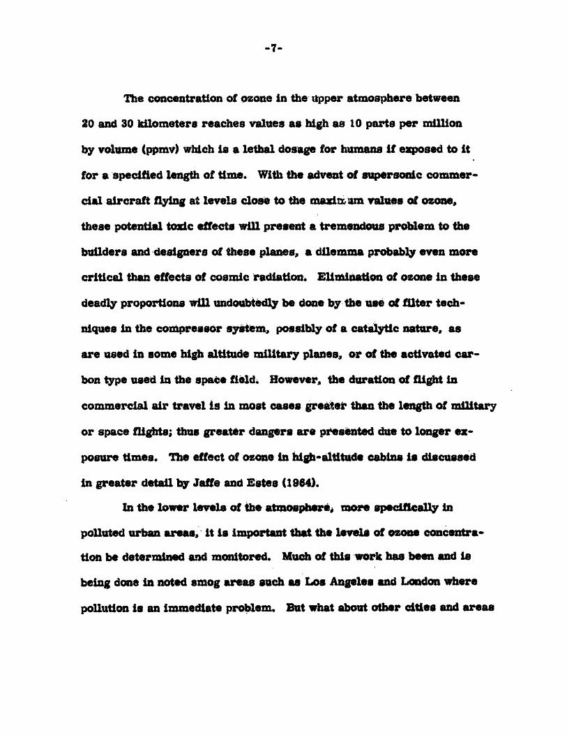
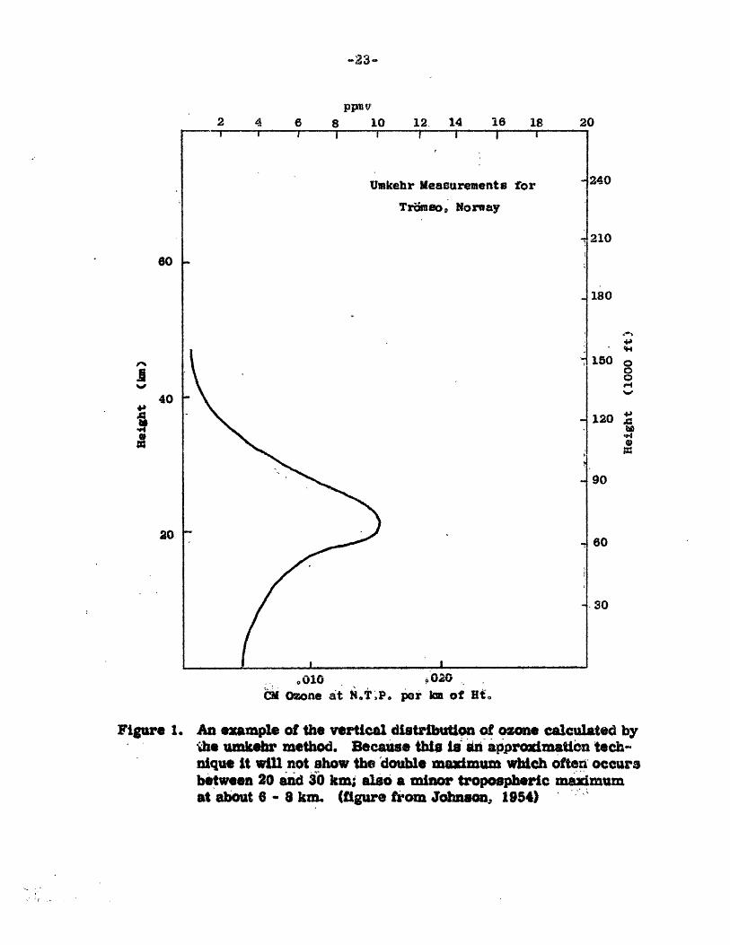
Figure 1. An example of the vertical distribution of ozone calculated bythe umkehr method. Because this i an approximation tech-nique it will not show the double maximum which often occursbetween 20 and 30 km also a minor tropospheric maximumat about 6 - 8 km. (figure from Johnson, 1954)

40

20

1240

210

180

150490

60

80

30

80

70

60

4 50

40

30

20

10

-410 0-310'

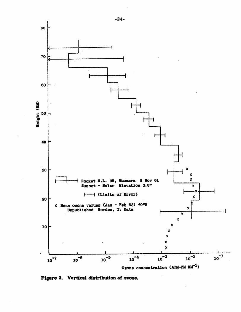
Ozone concentration (ATM-CM Io1 )

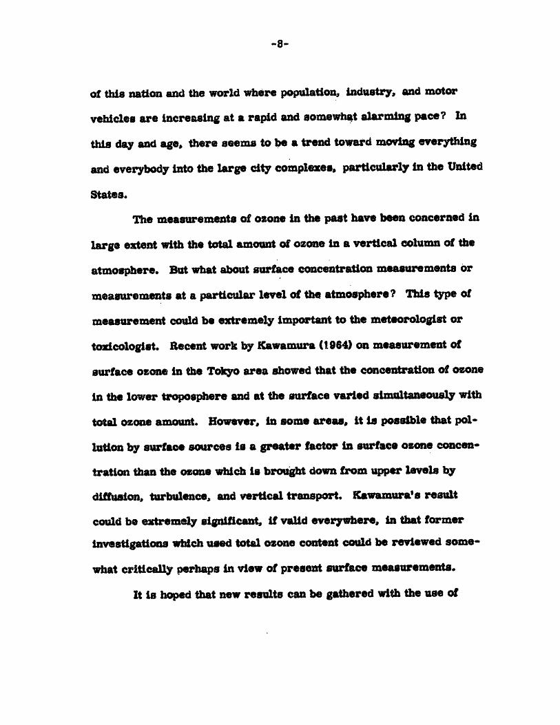
Vertical distribution of ozone.

I - Rooket 8.L. 35, Woomera 8 Nov 61Sunset - Solar Elevation 3.80

--- (Limits of Error)

K Mean ozone values (Jan - Feb 63) 40NUnpublished Borden, T. Data

10-

-24-

Figure 2.

clr J r i:

-25.-

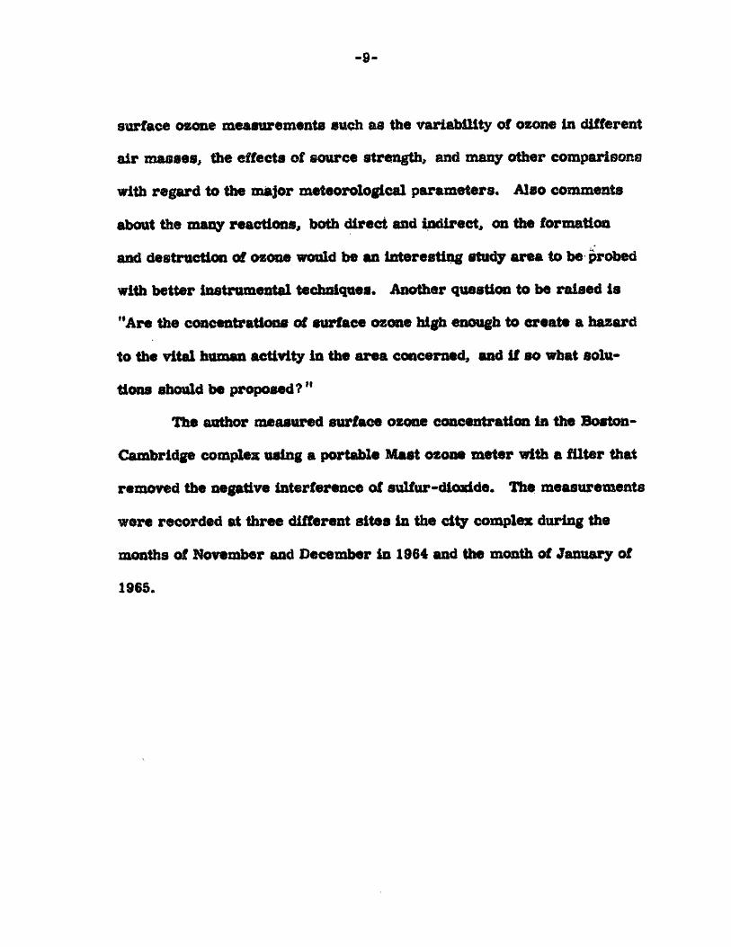
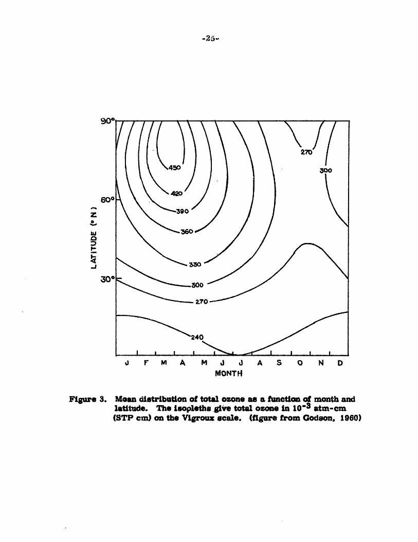
Figure 3.

F M A M J 3 A S O N DMONTH

Moean distribution of total ozone as a fuactoa of month andlatitude. The isopleths give total ozone in 10- 3 atm-cm(STP cm) on the Vigroux scale. (figure from Godaen, 1960)

-26-

a simiar interruption would take days to months to erase, and still at

lower altitudes, equilibrium is almost never restored. The reason

for this is that ozone absorbs so strongly in the ultraviolet wavelengths

which induce reactions that below the upper few kilometers, the atmos-

phere is protected from this light. In fact, in the Hartley band (3200-

2000 A), as low as 1/145 centimeter layer (STP) can reduce the inten-

sity by 11/10. The entire quantity of atmospheric ozone if reduced to

standard temperature and pressure would form a layer only a few

millimeters thick. Here, and in most other works on atmospheric

ozone, the concentration of ozone is given in terms of thickness. To

convert these units into parts per million by volume (ppmv), one needs

only the appropriate conversion factors (Appendix A).

B. Transport Properties

A circulation pattern of some type is needed which can create

a maximum of total ozone at the latitude and season at which it is found.

There are two immediate possibilities, one, a horizontal field of motion

which might concentrate it in a certaii band, or secondly, a vertical

motion which might pull down ozone from the region of photochemical

equilibrium. The actual field of motion is probably a combination.

Although we have a fairly good understanding of tropospheric

circulatIons, the fact that ozone is found mainly above 20 km forces

4 k. -

s to ,look to stratospheric motions to describe its behavior. In fact,

ozone is one of our better tracers to aid in the Investigation of the

stratosphere.

It is interesting to note that the early thinking on a stratospheric

general circulation followed the same pattern as the development of the

tropospheric circulation. Craig (1948) found the olone measurements

to indicate a mean meridional cell. However, a variety of data and a

many nvestigators, Reed (1953), Martin (1956), Diitsch (1959), Newell

(1963a, 1963), have led to a postulated circulation similar to the

troposphere, one in which the eddies play a major role in middle latitudes.

The work of Reed (1953) and that of Ditsch (1959) indicates that

there is a steady downward flux of ozone into the troposphere where it

is destroyed in large quantities by chemical, photochemical, and catalytic

reactions. The mechanism by which it is passed through the tropopauss

region is not thoroughly understood but the transfer apparently occurs

in the vicinity of the jet stream, in frontal zones, and perhaps also

directly across the tropopause region. These transfer processes have

been discussed by Danielson (1959, 1964), Brewer (1960), Staley (1960),

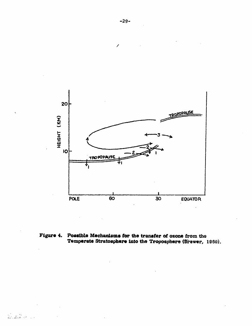
Newell (1968a) and Briggs and Roach (1963). The following presentation

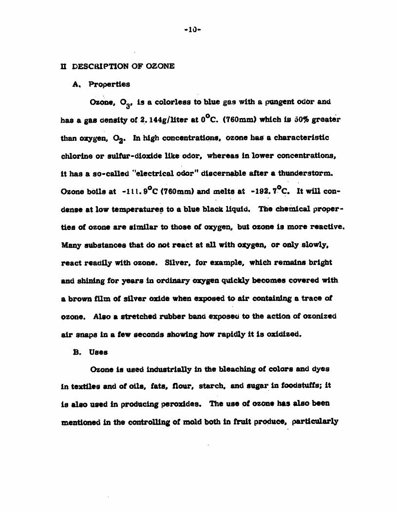
of four mechanisms is from Brewer's paper (see Figure 4):

1) Here is a continuation across the tropopause of the flow nonadia-

-28-

batic descent which is presumed to have brought the ozone down to the

tropopause. This process would tend to give a relatively uniform rate

of transfer of ozone into regions. The outflow would be greatest in

late Spring when the high concentrations are found near the tropopause.

2) Since the tropopause often slopes relatively to the isentropic

surfaces, especially in the region just north of the subtropical jet stream.,

motion along the isentropic surfaces can take ozone out of the strato-

sphere. This process would give greatest outflow just north of the sub-

tropical jet and requires relatively high concentrations of ozone just

above the tropopause in these regions.

3) Exchange can occur along the isentropic surfaces which lie in the

lower stratosphere of temperate regions and pass through the subtropi-

cal jet into the upper, tropical troposphere. Ozone-free air can enter

the stratosphere and conversely the ozone-rich air can pass out of the

stratosphere. This mechanism will concentrate outflow at the region

of the subtropical jet and will be greatest in Spring when the temperate

stratosphere contains most ozone.

4) There is also the possibility of this circulation pattern through

the lower stratosphere. Any contribution which such a circulation

makes to the transfer of ozone to the troposphere will give outflow in

the region of the subtropical jet with a strong maximum in late Spring

20

4

10 - -.ypOPPUSE

+

POLE 60

Figure 4. Possible Mechanisms for the transfer of ozone from theTemperate Stratosphere into the Troposphere (B8iewer, 1960).

-29-

30 EQUATOR__ _ _ ___ __ _ __

~I~

t---

i)t cr~)l*1

IrU. ~.

-so-

an, ear.y Srnmer when the ozone levels near the lower part of the jet

is highest.

For a more quantitative estimate of the relative importance of

the several transfer mechanisms based upon racioactivity data see a

Table by Machta, quoted by Murgatroyd (1964).

In conclusion to this section on ozone in the upper atmosphere,

the author feels that with more high-quality measurements, researchers

can look forward to a regular gri of reporting stations to aid in making

the study of atmospheric ozone a very valuable tool for the purpose of

further examination of the behavior of the stratosphere. Persons inter-

ested in present upper level ozone measurements are referred to the

compilation of data from the work of Mr. Wayne S. Hering (1964) at

the Air Force Cambridge Research Laboratories in Bedford, Mass.

Hering's data from ozonesondes from different stations over North

America give the ozone concentrations at various levels in the atmos-

phere rather than the total ozone amount in a column for the whole

atmosphere that was used in the studies mentioned in this section.

These reported and tabulated values make it easier to carry on investi-

gations at particular levels in the atmosphere with reliable and not

approximate wind data,

C. Lower Atmosphere (at the surface of the earth and particulary

i 4

-31-

in polluted air)

Tost of the ozone .resent in the atmosphere is produced photo-

chemically in the upper levels above 20 km as mentioned in the previous

sections; some of this ozone is transported downward into the troposphere

where it is partially destroyed by chemical reactions. The small amount

that reaches the surface of the earth is almost completely depleted by

the ozone reactions with surface soil, plants, etc. In this section, the

ozone production in the polluted surface layers particularly in the vici -

ity of urban areas will be discussed.

Ozone in polluted air is primarily produced and destroyed by

the following reactions according to Leighton and Perkins, 1958.

o 0

NOS + hv---NO + O (3100A < < 3700A) (5

O + O + M 0- O + M 2

O3 + hv--- Og + o

NO + 03 -- NO2 + o2 (

In (3) ozone absorbs between 2000 ana 3200 %in the ultraviolet

Hartley bands and between 4500 and 7000 X in the Chappius bands; how-

._i

.

ever all solar racdation of wavel1ngth shorter than 2900 is absorbed

in the upper atmosphere. M in (2) is any particle capable of absorbing

excess energy released by the reaction (otherwise 03 would be unstable

and quicily dissociate again). The atomic oxygen formed by (5) will aso

react with other constituents present in the polluted urban nQmosphere,

but the above mentioned authors reported that 99. 5% ot the atomic oxygte Y1

reacts with molecular oxygen to form ozone and that less than 0. 5% re-

acts by all other processes. Other reactions have been suggested-as

possible producers both directly and inoarectly of oone but their valid-

ity still remains uncertain.

While not immediately involved in the formation of ozone in pya-

luted air there are some constituents of the local air which enhance or

slow down the above main reactions. For example, ozone production

is apparently increased in the presence of olefins, whereas the prodaue-

tion rate of ozone for most paraffins is small as reported by Schuck

and Doyle (1959). Also some types of olefins not only promote rapid

rates of formation of ozone, but tend to promote high concentrations

of :zone. Reaction (2) is slow and does not substantially decrease the

ozone concentration but (3) limits the concentration which can cooxYot

with nitrogen-dioxide.

In view of the above reactions, one can easily see that the

~ A

-33-

prasence of nitrogen-oxides i very important in th~ sutdy of both uB~'an

and non urban pollution by ozone. The internal combustion engine and

other high temperature combustion processes such as industrial furnaces

are the chief sources of nitrogen dioxide, especially if the effluent$ ar-

rapidly cooled. Dickinson (1961) reports that with the gasolihae engine,

the nitrogen oxide is almost entirely in the form of nitric oxide when

exhausted from the engine; however, once in the atmosphere, nitric

oxide converts rapidly to nitrogen dioxide. According to Leighton and

Perkins, it appears that the conversion of nitric oxide to nitrogen di-

oxide is assisted by many organic substances such as olefins, aromati

hydrocarbons, aldehydes, and paraffins.

In a most recent work by Kawamura (1964), it is suggested that

a part of surface nitrogen-dioxide may originate from the surface soil

as a result of bacterial reaction. Kawamura also found from measure-

ments in Tokyo that nitrogen-dioxide in the surface air had a marked

duirnal variation with two maxima in the day which occurred respectively

in the morning three hours after sunrise and in the evening two hours

after sunset. This duirnal variation of nitrogen-dioxide in pollued air

could be explained as a result of meteorological conditions, photochem~-

cal effects, and traffic density. A similar result was found by Dickinson

(1961) in the Los Angeles area.

-34-

To show the importance of nitrogen-dioxide in the formation of

surface ozone, Vassy (t963) reported that the ozone concentration in

Paris was but a fraction (on the order of 1/10) of the concentration

measured in Los Angeles during comparable conditions. Most of this

difference was attributed to the smaller number of automobiles in the

French city; in a similar comparison between London and Los Angeles,

the ozone concentration ratios were in the same proportion as the en-

gine cylinder ratios. Other possible reactions of ozone with constitu-

ents of polluted air are those with members of the halogen family, most

important of which could be chloride. These particular chemical re-

actions will be discussed more completely in a later section of this thesis;

this evaluation is a direct result of this author's work in sampling ozone

in the Boston-Cambridge complex.

D. Other mechanisms in the production of ozone

In addition to the reactions mentioned in the previous three

sections, ozone is formed in other ways; one of these is the dissociation

of molecular oxygen into atomic oxygen by an electrical discharge and

the subsequent reaction of the Oxygen atom with molecular oxygen to

form ozone. In the atmosphere, this is a common occurrence during

lightning in thunderstorms, discharge from airplanes, and even in

silent discharges that happen in snowstorms. Vassy (1954) showed

-35-

while measuring surface ozone in Paris that there is a definite In-

crease in concentration during thunderstorms; however, the abrupt in-

crease of this concentration occured three and one-half hours before

the first discharge on the average. It is the opinion of Kroening and

Ney (1962) that ozone produced by lightning is on the same order as

that produced by solar ultra-violet light.

Another ozone production method discussed by Kroening and

Ney is of nuclear origin; they calculated that the amount of ozone pro-

duced by a fifty megaton nuclear device is approximately 0. 1% of the

ozone in the entire atmosphere.

There is also a production related to the presence of aerosols

as reported by Reshetov (1961). Here, the reaction of water and oxygen

(in air) due to selective adsorption on the surface of the aerosol parti-

cle forms hydrogen-peroxide; the reactions that follow are discussed

in full by the author and will not be repeated here. Reshetov's proposal

stems from many so-called unexplained facts on ozone; one of which

was the report of high ozone content near waterfalls and in the vicinity

of sea sprays as measured by Leybinzon (1936). All of the facts except

the one above ean be explalei by onventional neans; however, the

present author feels that measurement techniques at that time were

questionable. Regener (1954) considered atmospheric aerosols to be

a scavenger but not generator of ozone and conceded that the photo-

chemical diesoclation methcod are probably the rost important.

-37-

V INSTRUMENTATION

A. Ozone measuring devices

Ozone can be measured by two techniques, spectrophotometric

or chemical; the former has been used mostly for total ozone (Appendix

A) as well as vertical distribution, and this "umkehr effect" is discussed

in detail by Mitra (1952) or Johnson (1954). Mateer (1964) concluded

that there is no possibility of determining fromumkehr observations

whether or not there exists a distinct secondary maximum in the lower

stratosphere. He also states that the vertical distributions of ozone

obtained from umkehr observations are to be compared with each other

oy Kwhen determined by the same objective technique. Great care must

be taken when making inferences about atmospheric motions from ver-

tical distributions of ozone obtained from umkehr obsevations since

the evaluator sometimes uses subjective methods on what the vertical

distribution "should" look like.

Chemical methods of ozone determination go back 100 years when

measurements were made in the layer of the atmosphere closest to the

earth in Germany with the use of Schonbein's potassium iodide starched

paper. Dauvillier in 1933-35, used a reaction of the oxidation by ozone

with a titration solution of sodium arseenite to measure the ozone. The

ozone amount was determined by the portion of the solution which remains

-38-

unxidized. This portion was titrated with an iodine solution, Also

at this time, a rubber cracking method was used, but this was an em-

perical scheme in that it was not specific to ozone and had to be Inter-

preted with caution; the technique was a cumulative test for total sub-

stances in the attnospbere effecting rubber (Jacobs, 1960).

In the last two decades, great improvements have been made

on the potassium iodide method for ozone determination, and also a new

method, oxyluminescence, was discovered. At one time, a colorimet-

ric analysis was used, whereby the products of the reaction were

usually determined by comparison of the color of the indicators at a

certain stage of the reaction. For example, oxidation by ozone of solu-

tions of potassium iodide and other odides are accompanied by an in-

crease in the solution of the etfective concentration of bydrogen tons

(an increase of the pH). This kind of reaction leads to the use of color

indicators such as phenol, bromotbymol, nirtophenol, phenolphthalen,

and others for the qualitative determination of high ozone concentrations

in the air. Here, absolute values of the ozone concentration can be ob-

tained by comparing the action of each indicator in a pecific schedule

of measurements with one of the absolute methods of measurements of

the ozone. Another example of the colortmetric method is the reaction

of the oxidation by ozone of Indigo. earmne, a substance used by Britayev

-39-

(1959) in a number of cases for a qualitative evaluation of comparatively

high ozone concentrations in the atmosphere, The ozone concentration

is calculated by the equation of the chemical reaction and by the amount

of air passed through the solution. In spite of the simplicity of the color-

imetric analysis, it still involves the subjectivity of the estimation of

the color alteration, and this is its most important fault.

Ozone causes luminescence in contact with several chemical

elements (iodine, sulphur, sodium, thallium), mineral compounds (the

sulphides, the chlorides, and also an oxide of nitrogen), sea water,

milk, and also chlorophyll. Very strong luminescence can be observed

when ozone acts on luminol in an alkaline solution. Bernanose and

Rene (1959) determined the ozone concentration by the intensity of oxy-

luminescence. However,. a small amount of moisture is essential for

this chemiluminescent reaction to take place in luminol. Regener

(1964) used the chemiluminescent reaction between ozone and rhodamine

B which does not show this type of moisture effect, His instrument in

balloon-borne sonde equipment is used widely in investigations n the

upper atmosphere over North America.

The basis for the majority of presentday electrochemical

methods of ozonometry is the reaction by ozone of potassium iodide in

aqueous solution,

03 + 2K1 + H20 ---- 12 + 02 + 2KOH

The reaction with potassium Iodide is characterized by great selectiv-

ity with regard to ozone. Exact quantitative measurements of ozone

are effected by electrochemical methods. wherhe reaction of the

destruction of the ozone is checked by the alteration of the electrical

properties of the solution being oxidized by the ozone. The instrument

chosen by this author for study of the air in the Boston area was the

Mast ozone meter (Mast and Saunders, 1962). This particular instru-

ment was chosen for its simplicity of operation, ease of handling cost,

and most important the quickness in obtairfng the instrument for im-

mediate use. - In this instrument, the above chemical reaction takes

place on the cathode portion of an electrical support. At this cathode,

a thin layer of hydrogen gas is produced by a polarization current:

2e + 2H --- * B 2 (8)

When the voltage is applied to the electrodes (0. 24 volts), the hydrogen

layer builds to its maximum, and the polarization current ceases to

flow, When free iodine Is produced by the reaction with ozone, it re-

acts immediately with the H 2 as follows:

H3 + I2 -- 4 2HI

(7)~

(9)

-41-

The removal of hydrogen from the cathode causes a re-polarization

current of two electrons to flow in an external circuit, re-establishing

equilibrium. Thus, for every ozone molecule reacting in the senso,

two electrons flow through the external circuit. Hence, the rate of

electron flow, or current, is directly proportional to mass per unit

time of ozone entering the sensor. The instrument was connected to

a recorder which was calibrated in pphmv (part per hundred million

by volume) and could be read directly when the air flow rate was 140

ml/main at STP. To correct for ambient conditions and thus get a

more accurate reading the instrument values should be multiplied by

p (_ambient) T (standard)a factor of p (standard) T (ambient) The uncertainty or accuracy

of the instrument is reported to be I ppbv (parts per billion by volume)

which is approximately the limit to which the graph on the recorder

can be read. Further information desired. about the Mast ozone meter

and recorder can be obtained from the Mast Development Company,

Davenport, Iowa.

B. Disturbing agents in the electrochemical (KI) method of ozoneanalysis (use of filter)

When considering the measurement of ozone by the electro-

chemical method with a potassium iodide solution, one should be aware

of possible Interference from oxidizing or reducing agents or erroneous

readings from other means, Possible interfering agents, mostly

-42-

found in polluted air are sulftr dioxide (S02), nitrogen dioxide (NO2)

and nitrate ion (NO;). There is also possible destruction of ozone

from the wall-effect of g tubing (Kawamura, 1964) which is used

as an air inlet by many authors and researchers; however, in this

taudy of Boston air, a polyethelene and teflon tubing was used for inlet

air intakes.

Of the above mentioned contimnants, sulfur dioxide is the most

important. Saltzman and Wartburg (1964). Ripperton (1964), and

Kawamura (1984) all reported on the negative interference of this gas-

eous substance common in polluted or urban atmospheres; but only the

first two authora suggested a mean.tor removal of 802 from the air

nlet so as to improve the accuracy of iodometric measuring devices

such as the Mast instrument. Their method is as follows: Prepare

a 10 ml solation containing 83 - 1. 66 grams of chromium troixide

and .46 -. 93 cc concentrated sulphuric acid. Drop solution (with

eyedropper) onto 6 sq. in. ot glass fiber filter paper; dry paper in

oven at 80oC for one hour or until paper turns pink (in my case, this

happened in approximately one half hour). Now, cut dried filter paper

into 1/4 by 1/2 inch pieces and told the pieces into V shapes. Place

the folded paper into 100 mm Schwars U tube (glass). ( used a 100

mm straight polyethelene tube). The paper (pie shaped because I used

-43-

circular filter paper, 1 in. diameter) was folded to prevent nesting to-

gether when packed in the tube. The final product resembled a large

cigarette type filter and acted in essentially the same manner. Con*

ditioning of the filter and also ensuring against any blocking of the air

intake flow was accomplished by drawing laboratory air through the

filter with the aid of a small vacuum pump. The theory of this filter

technique to based on the fact that the chromium trixide is an excel-

lent oaidi ng agent; thus the sulfur dioxide a oaidized to S03 (highly

hygroscopic) which then clings to the glass fiber filter paper. Saltzman

and Wartburg (1964) report that the filter is good for thirty days and

are stil in the testing phase for longer periods of time.

Nitrogen dioxide (NO2 ) interfere positively on the instrument

to the order of from one to ten percent of the amount of NO2 present

depending on whether one uses Kawamura's or Ripperton's figures.

Junge (1063) gives typical values of NO 2 of approximately 15jfg/m3

( . 7pphm) for large urban areaq whereas for Tokyo, Kawamura reports

maximum readings of 78 /g/m 3 (3 pphm). It maximum error is used,

one gets only values of .07 pphm or 0. 3 ppbm which are very small

compared to actual readings of ozone; in fact, these figures are the same

magnitude as the reported accuracy of the instrument. Also, the use

of a buftered potassium iodide solution (this is used in Mast instrument)

-44-

tends to reduce the effect of NO 2 even more; so no problems were to

be encountered in this aspect of the study.

The disturbing effect due to the presence of the nitrate ion (NO3)

In the atmosphere is negligible as reported by Kawamura (1964) in his

research report of pollution n the Tokyo area.

VI SELECTION OF THE SAMPLING SITES

The ozone concentration data reported in this study represent

measurements with a portable Mast ozone meter taken at three types

of sampling sites. It was decided to choose one location near a major

traffic thoroughfare and another a short distance away elevated above

the street level; these locations should be in the heart of a city com-

plex. A third site should be away from the city, i. e., in the suburbs,

so as to have a sample of non-urban classification. In addition to the

above restrictions, several other practical considerations were met

in the final selection of the three sampling sites. The first two sites

mentioned should be close enough together to represent the same con-

ditions of industry and traffic density. All the sites should be near an

outlet for electrical power to drive the ozone meter. Luring the curb-

side period of the test, the operator must remain on site to take and

record various readings of meteorological and traffic conditions and

to safeguard the equipment against possible interference by over-

curious passers-by. Therefore, the curb-side site should allow legal

parking to permit the operator to employ his vehicle as a base of opera-

tions and a place of temporary storage for the equipment directly and

indirectly involved in the test.

The sites actually chosen for this test meet the above criteria

-45-

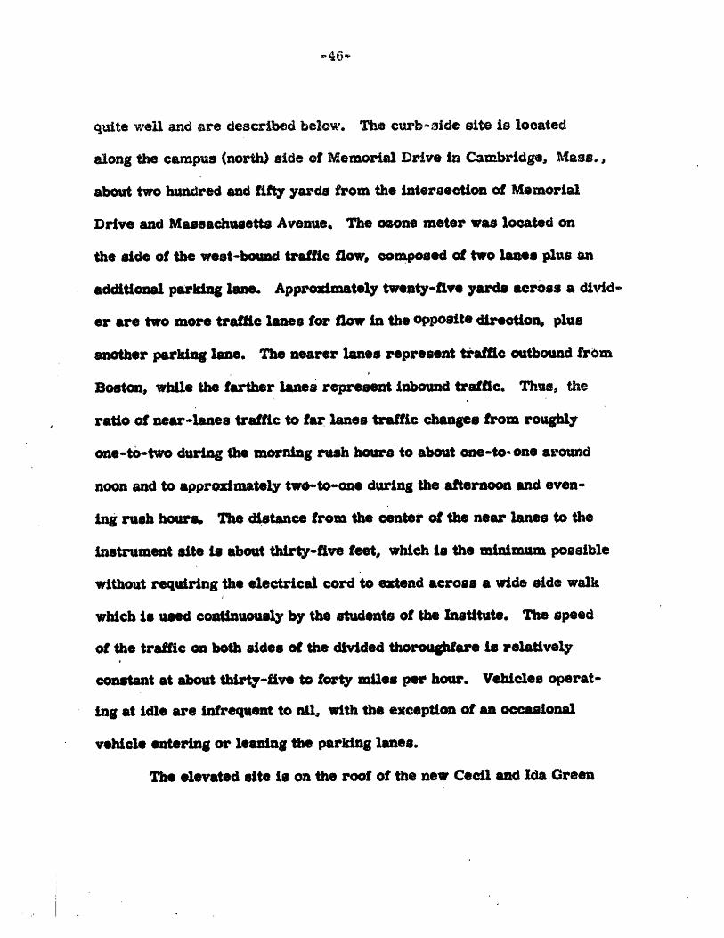
quite well and are described below. The curb-side site is located

along the campus (north) side of Memorial Drive in Cambridge, Mass.,

about two hundred and fifty yards from the intersection of Memorial

Drive and Massachusetts Avenue. The ozone meter was located on

the side of the west-bound traffic flow, composed of two lanes plus an

additional parking lane. Approximately twenty-five yards across a divid-

or are two more traffic lanes for flow in the opposite direction, plus

another parking lane. The nearer lanes represent traffic outbound from

Boston, while the farther lanes represent inbound traffictl. Thus, the

ratio of near-lanes traffic to far lanes traffic changes from roughly

one-to-two during the morning rush hours to about one-to-one around

noon and to approximately two-to-one during the afternoon and even-

ing rush hours, The distance from the center of the near lanes to the

instrument site is about thirty-five feet, which is the minimum possible

without requiring the electrical cord to extend across a wide side walk

which is used continuously by the students of the Institute. The speed

of the traffic on both sides of the divided thoroughfare is relatively

constant at about thirty-five to forty miles per hour. Vehicles operat-

ing at idle are infrequent to nil, with the exception of an occasional

vehicle entering or leaning the parking lanes.

The elevated site is on the roof of the new Cecil and Ida Green

iib r

Center for Earth Sciences, on campus approximately two hundred

yards from the curb-side site. The exact location of the meter on

the roof depends on the wind. That is, it is almost always positioned

upwind of the laboratory hood exhaust and the air conditioning cooling

water spray, either of which might act as a contaminant source with-

out suitable precautions.

The third and final site is the author's home in Roslindale,

approximately ten miles southwest of the Cambridge-Boston complex.

The Instrument was placed n an upstairs (2nd floor) room about 25

feet above the ground with the inlet tube sticking out of the window.

The author intended to alternate the meter equally between the urban

and suburban, sites but the severe weather (specifically strong winds)

necessitated the sheltering of the instrument.

~Y~Y). % ~!d~~ :-

VII DISCUSSION OF RESULTS

A. aOzone Measurements in the Boston-Cambric ge Complex

The following results were recorded and computeo from the

ozone measurements at the three sampling locations; specifically, the

November data was obtained from the roof-top locality with fifteen

hours of curb-site measurements interfused, while the December and

January values were taken from the third sampling site mentioned

(less than ten miles from the other two) with approximately three days

of roof-top site recordings intermingled. While it is difficult to make

any defendable conclusions on the effects of the change of location, be-

cause there are no samples taken an all locations simultaneously or

under completely equivalent weather conditions, it is felt that since the

measured substance is gaseous, a thorough mixing at low levels near

the surface is a reasonable assumption. This postulate was borne out

somewhat; for in the several instances when the instrument and record-

er were transferred between sites (transfer time less than one hour),

the recorder values of ozone concentration did not change in this site

to site transferrence.

The monthly means were computed by averaging ono hour means

for the entire month concerned. This was a tedious operation because

one inch of the trace on the recorder paper corresponded to one hour.

':''

(I l9)~1 01I I I I

9 c 0 qe S ozZL39WIMXst 01>R- ~

~

MW3AONQ1 01

II I I I I I

0V~70Q0

0

* 00v

weVOO

00C

0V

00

00

v 0

00

V

7

(ss~a i't-OT IOU) SOUMl 40 I1ZflnO IT.na XV

(,,- P1-31) OJtrIO4 uOQU SuTinp POAJZTIOO ;T oDSa-3P~Tqm'3 uO4808) sIO2O aoe;fl19

JO 8-sr'1TA £lTvuc UnRflm~f

00

00

12

oz

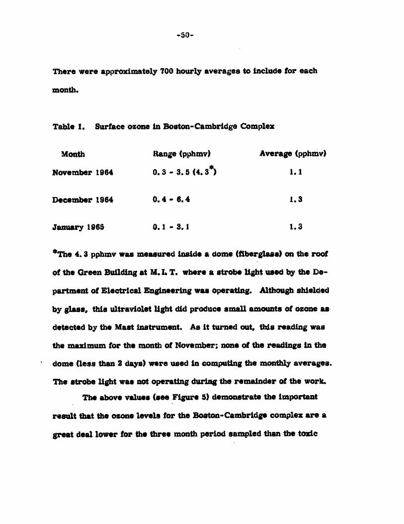
There were approximately 700 hourly averages to include for each

month.

Table 1. Surface ozone n Boston-Cambridge Complex

Month Iange (pphmv) Average (pphmv)

November 1964 0. 3 - 3.5 (4. 3") 1. 1

December 1964 0. 4- 6. 4 1. 3

January 1965 0. 1 - 3. 1 1. 3

*The 4. 3 pphmv was measured inside a dome (fiberglass) on the root

of the Green Building at M. I. T. where a strobe light used by the De-

partment of Electrical Engineering was operating. Although shielded

by glass, this ultraviolet light did produce small amounts of ozone as.

detected by the Mast nstrument. As it turned out, this reading was

the maximum for the month of November; none of the readings in the

dome (less than 2 days) were used in computing the monthly averages.

The strobe light was not operating during the remainder of the work.

The above values (see Figure 5) demonstrate the important

result that the ozone levels for the Boston-Cambridge complex are a

great deal lower for the three month period sampled than the toxic

levels for humans, animals, and plants as discussed in an earlier

section of this thesis (section III). Since the months of the measure-

ments nclude the time of year when insolation and total ozone in the

atmosphere are at a minimum, it would be worthwhile to measure

surface ozone during the time of maximum insolation (Summer) and

the time of maximum total ozone (Spring). Such a complementary

study is being carried out by a colleague in the Meteorology Depart-

ment. However, it just might be that though the amounts of ozone in

this future report will probably contain higher concentration levels,

the values could still be much lower than potentially hazardous ones.

This does not mean that measurements of surface ozone should then

be discontinued with regard to this aspect of the results. On the con-

trary, measurements of low level ozone along with other pollutants in

the urban air should be taken periodically over the years to insure that

the concentrations reached remain at these same low levels.

B. Past Measurements

As is the case with any study in which measurements, particu"

larly of very small quantities, of a substance are reported, it is almost

always necessary, if possible, to Include past measurements of the

same substance it only for a comparison of the relative magnitudes.

In the measurement of surface or low level ozone, there are slight prob-

lems however; first of all, not too many reports of measurements of

surface ozone exist in the literature, and secondly, in the majority of

measurements that were reported, the researchers did not use tech-

niques which were specific to ozone. In the discussion presentea here,

the author considers only studies in the last 15 years, for it is only

since then that fairly reliable methoos for surface ozone analysis have

appeared. If the instrumentation had failings or shortcomings in this

period, the researchers were essentially aware of them.

Measurements at the surface in the Los Angeles Basin reported

as total oxidant by ienzeth (1954) were as follows. At night, the

values averaged between 2 and 4 ppbmv. The average maximum con-

centrations for the entire area during the month of November, 1954

were from 7 to 15 pphm(v).

Measurements of surface ozone reported by Cauer (1951) for

locales throughout Europe during the years 1949 to 1951 had a range

from 0 to 9. 5 pphm(v). Most of these measurements were obtained

with an Ehmert electrochemical (potassium iodide) technique.

Kawamura's measurements for the Tokyo area were obtained

by the same method as reported by Cauer with only minor modifications,

The values reported for Tokyo during 1958 and 1959 showed a range

from I to 3 pphm(v).

Of all the measurements reviewed by this author, the three

mentioned below used the Regener Rhodamin B chemiluminescent tech-

nique which is specific to ozone.

Kroening and Ney (1961) measured surface ozone in Minneapolis,

Minnesota during the month of May and reported daytime values of

approximately 2 pphm(v) with minor fluctuations; nighttime values were

generally 11/30 of the daytime values.

Ripperton (1984) in analyzing seventeen 24-hour samples taken

over a period of one year in Chapel Hill, North Carolina, reported

ranges from 0.0 to 13 pphm(v). The nighttime range was 0. O0 to 0. 1

pphm and the daytime range was 6. 4 to 13. 0 pphm(v).

Finally values computed from Bering's data for the month of

December, 1962 taken in mid-afternoon showed a range of .8 to 2. 7

pphm. These values were for approximately a height of three-hundred

feet, the same height as the Green Building at M, I. T., and represented

the first level of the measurement of the ozonesonde run for Bedford,

Massachusetts.

Of course, the measurements discussed in the preceding para-

graphs are not going to be exactly the same as this author's measure-

ments in the Boston-Cambridge complex because of variation due to

geographical location, time of year, year, and pollutant sources, etc.

But it is. most gratifying in an investigation of a small concentration

-54-

substance like ozone in surface air to find that one's results are not

drastically different from others reported.

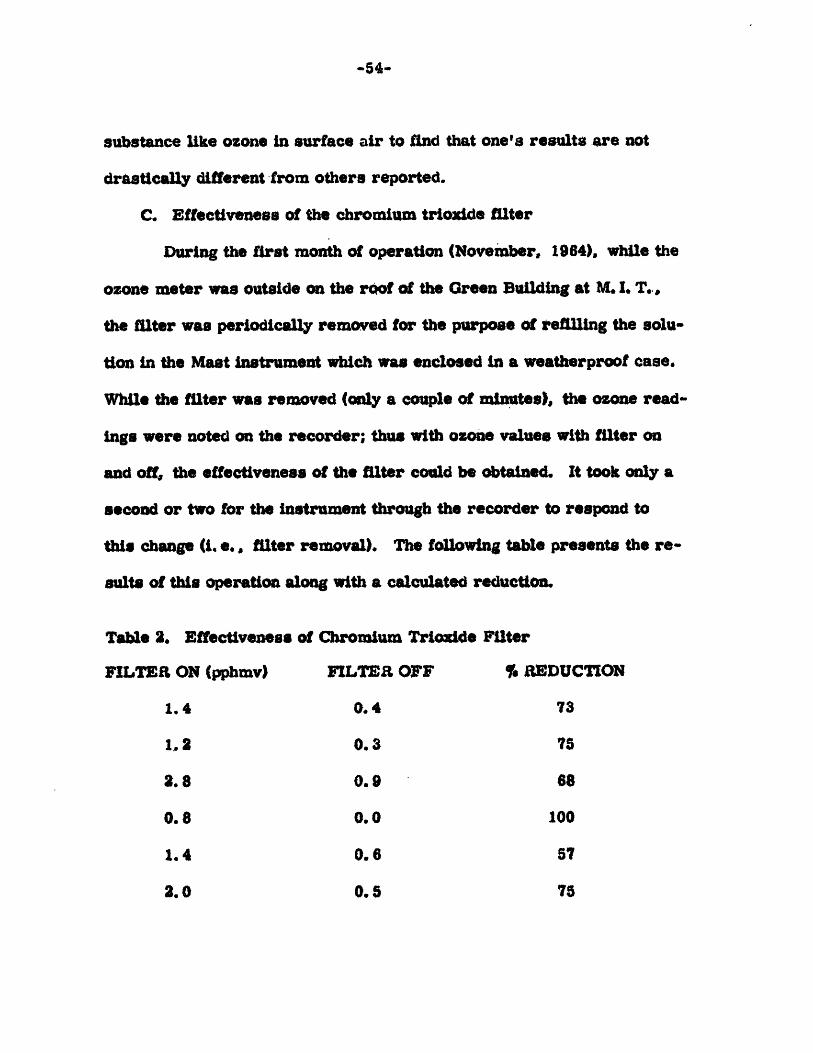
C. Effectiveness of the chromium trioxide filter

During the first month of operation (November, 1964). while the

ozone meter was outside on the roof of the Green Building at M. I. T.,

the filter was periodically removed for the purpose of refilling the solu-

tion in the Mast instrument which was enclosed in a weatherproof case.

While the filter was removed (only a couple of minutes), the ozone read-

ings were noted on the recorder; thus with ozone values with filter on

and off, the effectiveness of the filter could be obtained. It took only a

second or two for the instrument through the recorder to respond to

this change (i. e. , filter removal). The following table presents the re-

sults of this operation along with a calculated reduction.

Table 2. Effectiveness of Chromium Triozide Filter

FILTER ON (pphmv) FILTER OFF %a REDUCTION

1.4 0. 4 73

1,.2 0.3 75

. 8 0.9 68

0.8 0.0 100

1.4 0.6 57

2.0 0.5 75

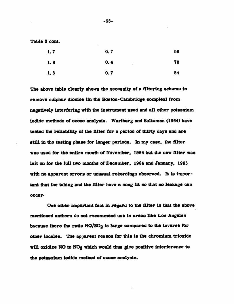
-55-

Table 2 cont.

1.7 0.7 59

1.8 0.4 78

1.5 0.7 54

The above table clearly shows the necessity of a filtering scheme to

remove sulphur dioxide (in the Boston-Cambridge complex) from

negatively interfering with the instrument used and all other potassium

iodide methods of ozone analysis. Wartburg and Saltzman (1964) have

tested the reliability of the filter for a period of thirty days and are

still in the testing phase for longer periods. In my case, the filter

was used for the entire month of November, 1964 but the new filter was

left on for the full two months of December, 1964 and January, 1965

with no apparent errors or unusual recordings observed. It is impor-

tant that the tubing and the filter have a snug fit so that no leakage can

occur,

One other important fact in regard to -the filter is that the above

mentioned authors do not recommend use in areas like Los Angeles

because there the ratio NO/SO2 is large compared to the inverse for

other locales. The apparent reason for this tois the chromium trioxide

will oxidize NO to NO2 which would thus give positive interference to

the potassium iodide method of ozone analysis.

L Discussion of results with respect to

1. Past Measurements

In comparing my surface ozone measurements with past

measurements (section B), a few interesting comparisons were noted.

First of all, the closeness of Hering's values taken in Bedford during

the same months as in this study although a different year was partic-

ularly important to this researcher. Secondly, the Los Angeles values..

also for the same months, but different year, were approximately 6

times the Boston-Cambridge values, both for daytime and nighttime

levels. This was to be expected because of the intensity of the well-

known ozone enriched smog so prevalent in the California city. A

third slightly unusual comparison was noticed between the Minneapolis

values reported by Kroening and Ney and the Boston-Cambridge measure-

ments. The size and human activity of both cities are nearly the same,

but the month and year of ozone comparison are different. Even though

the daytime concentrations of both locales were almost the same, a

striking difference in the nighttime values was present. The nighttime

concentrations of ozone in Minneapolis were approximately 1/30 of

their daytime values; in Boston, the nighttime levels were generally 1/6

of the concentrations reached in the daytime. Could it be that the de-

struction of surface ozone at night in the Minnesota city is greater due

-56-

L ~J

to time of year, temperature, or other local mechanisms ? The Los

Angeles ratio of nighttime to daytime values was nearly the same as

Boston.

2. Meteorological factors

Cholak tala(1956) measured surface ozone using a Beckman

potassium iodide method in ten eastern U. S. cities. They concluded

that the levels of ozone concentration were too low and too dependent

on sulphur dioxide to be reliably correlated with meteorological

variables. This was not the case in the presented study where sulphur

dioxide was filtered from the instrument, and the ozone variation was

significantly discernible.

In an examination of wind direction dependence, there were

only a few days whereby completely satisfying requirements existed

for this relationship; that is nearly the same weather conditions (cloud

cover, air mass, etc) with a strong wind directional change. In this

period (November 7-8), it was noted that with a northwest wind, the

ozone levels were less than those which occurred with a west or south-

west flow. This difference (a factor of approximately two) can prob-

ably be explained in that many pollhtion sources (cities, industrial

areas) are located in these directions whereas to the northwest few

sources exist.

-574

It was also decided to examine the possible ozone pollution

content with air masses since air masses are roughly internally

homogeneous with respect to temperature, moisture content, etc. In

analyzing the ozone variation across fronts, no apparent recognized

variability was noticed between the air masses. However, in the frontal

zones, where considerable overturning of the air is present, consider-

able fluctuations of ozone levels occured; sometimes the levels came

close to daytime values, when fronts passed during the night. These

fluctuations also happened with strong surface winds and rapidly chang-

Ing wind directions; all these conditions are conducive to low level

turbulence and will be discussed in the next section, source strength.

Most often, in a study of air pollution, researchers use rawind-

sonde data to make estimates of the degree of dynamic stability or in-

stability present in the atmosphere. (See Willet and Sanders (198589)

for complete discussion). The data is obtained from a nearby Weather

Bureau station that participates in the atmospheric sounding network.

Robinson (1961), however, advises caution in assuming that data

from soundings taken outside the area of an urban pollutant sampling

location can adequately represent the temperature structure over a

city, in view of the thermal modifications imposed upon the atmos-

phere by the presence of the city itself. With no vertical temperature

difference measurements available, a different parameter must be

used. My colleague R. L. Lininger, (Appendix B) used the following

technique; and since a small part of my study was done in conjunction

with his work, it was decided to discuss this method here as a guide*

line for future researchers. While the values for this relationship

will be presented, no conclusions are to be expected because it was

such a small sample. Turner (1961) used this index which he attributed

to the work of Dr. F. Pasquill. The method of computation is describ-

ed briefly below, omitting some of the details.

First, one obtains the solar elevation angle a, which is given

by the following equation for daytime observations:

a sin-1 in L sin D + cos L cos D cos H]

where L * the latitude of the sampling location

H a the hour angle, computed from local noon at the rate of 150per hour

D a the declination angle of the sun, available in tables, as aftnction of time of year. See List (1951).

From the solar elevation angle, one obtains an insolation class number

which is modified semi-objectively for sky conditions. This modifica-

tion gives what is termed the net radiation index. (Special rules apply

at night, but no night observations are ncluded in this report). Then,

_ i ' -

, , '

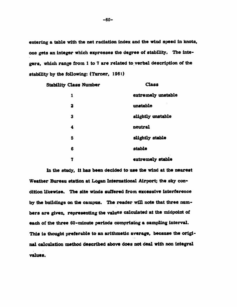
entering a table with the net radiation index and the wind speed in knots,

one gets an integer which expresses the degree of stability. The nte-

gers, which range from 1 to 7 are related to, verbal description of the

stability by the following: (Turner, 1961)

Stability Class Number Class

1 extremely unstable

2 unstable

3 slightly unstable

4 neutral

5 slightly stable

6 stable

7 extremely stable

In the study, it has been decided to use the wind at the nearest

Weather Bureau station at Logan International Airport; the sky con-

dition likewise. The site winds suffered from excessive interference

by the buildings on the campus. The reader will note that three num-

bers are given, representing the values calculated- at the midpoint of

each of the three 60-minute periods comprising a sampling interval.

This isto thought preferable to an arithmetic average, because the origi-

nal calculation method described above does not deal with non integral

values.

-60-

-61-

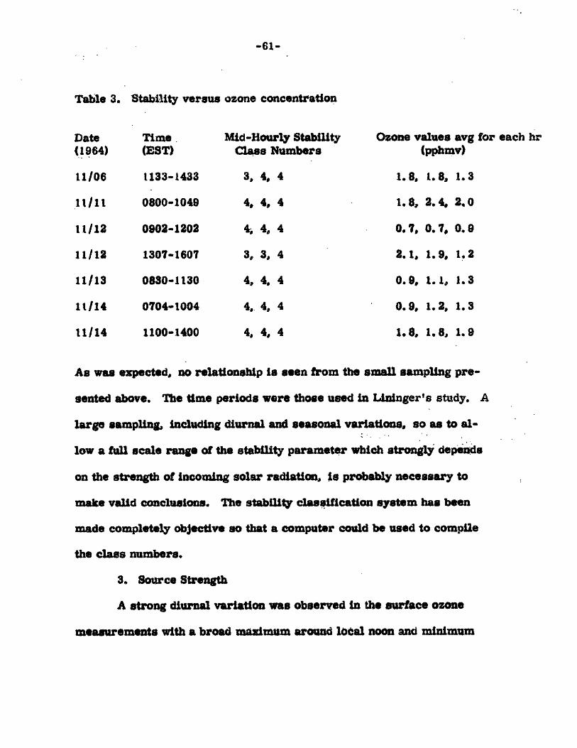
Table 3. Stability versus ozone concentration

Time .(EST)

1133-1433

0800-1049

0902-1202

1307-1607

0830-1130

0704-1004

1100-1400

Mid-Hourly StabilityClass Numbers

3, 4, 4

4, 4, 4

4i 4, 4

3, 3, 4

4, 4. 4

4, 4, 44, 4, 4

Ozone values avg(pphmv)

1.8,. 1. 8, 1.3

1.8, 2.4 2.0

0.7, 0.7, 0.9

2.1, 1.9, 1.2

0.9, 1.1, 1.3

0.9, 1.2, 1.3

1.8, 1.8, 1.9

for each hr

As was expected, no relationship is seen from the small sampling pre-

sented above. The time periods were those used in IAnnger's study. A

large sampling, including diurnal and seasonal variations, so as to al-

low a full scale range of the stability parameter which strongly depends

on the strength of incoming solar radiation, Is probably necessary to

make valid conclusions. The stability classification system has been

made completely objective so that a computer could be used to compile

the class numbers.

3. Source Strength

A strong diurnal variation was observed in the surface ozone

measurements with a broad maximum around local noon and minimum

Date(1964)

11/06

1112

11/12

11/13

11114

11/14

values during the night. At sunrise, the ozone generally increased and

then decreased at sunset. This diurnal variation was more pronounced

during days of excellent weather conditions (clear with no visibility re-

strictions). This observation agrees somewhat with the study by McKee

(196 a in Greenland where he reported measurable quantities of surface

ozone disappeared when the sun was obscured by high level clouds. With

low level clouds present, stability as well as photochemical dependence

would be an important factor. However these results are not entirely

analogous to high ozone concentrations as found with smog conditions

in Los Angeles. This is probably due to the difference of pollutants

present in the California city compared with our area where the smoke,

haze, etc. does not contain much ozone or precursors of ozone.

From Table 1, the monthly means show an increase, a trend

that is similar to total ozone amounts which are a minimum in the Fall

increasing to a maximum the following Spring. However, a longer per-

iod of measurement of surface ozone would be necessary to show absolute-

ly the strong dependence on total ozone rather than local pollution.

During the nighttime hours, when surface winds were strong

( > 10kts) and gusting, sudden increases in the surface ozone concen-

trations were recorded. These levels occasionally approached the high-

er daytime values. These are called turbulent interludes discussed by

-63-

Blackadar et al (1961) where the vertical gradient of wind velocity

suddenly becomes disturbed by the creation of turbulence which produces

a connection between the surface and higher velocity winds hundreds of

feet above the ground. This phenomena also occurred during strong

wind shifts, in frontal. zones and when an upper level trough was located

east of the sampling site (subsidence effect). During these turbulent

interludes, one could then assume that the ozone aloft (above the inver-

sion) is brought to the surface by the increased eddy difftsion and sub-

sidence. The above comments are discussed in a qualltative nature

because of the difficulty in expressing these factors in a quantitative

way and correlating them with the many other variables that come into

play on surface ozone values.

Peak surface ozone values versus the concentration of radio-

active substances in surface air ( j activity) are presented in Figure

6 since both have the lower stratosphere as an ultimate source region.

Notice the similar trend particularly in the early weeks of the study.

Finally, a brief table of ozone versus traffic density is offered

here. The results were obtained from joint work with R. L.. Lininger

(Appendix B). The measurements were taken at the curb-site.

5 day averages of peak SFC ozone concentrationveraus P (beta activity) from Public Health Service

X SFC Ozone (Boston-Cambridge)

A (Lawrence, Mass.)

O (Winchester, Mass.)

(N) No. of days other than 5

(3)

Q0.O

U

0.2

CI)(4)

1-5 6-10 11-15 16-0 PJ-25 26-30 1-5 6-0November. (1964)

Figure 6. Peak ozone versus beta activity in

11415 16-20 21-25 23ZI 1-5December i1964)

surface air

6-10 11-15 16-aO 21-5 26-31January (1965)

(4

.60

.50

.40

I I I I _

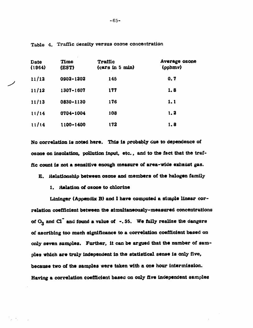
Traffic density versus ozone concentration

Date Time Traffic Average ozone(1964) (EST) (cars in 5 min) (pphmv)

11/12 0902-1202 145 0.7

11112 1307-1607 177 1.8

11/13 0830-1130 176 1. 1

11/14 0704-1004 108 1.2

11 / 4 1100-1400 172 1. 8

No correlation is noted here. This is probably drue to dependence of

ozone on insolation, pollution input, etc., and to the fact that the traf-

fic count is not a sensitive enough measure of area-wide exhaust gas.

E. Relationship between ozone and members of the halogen family

1. relation of ozone to chlorine

Linnger (Appendix B) and I have computed a simple linear cor-

relation coefficient between the simultaneously-measured concentrations

of 03 and C1 and found a value of O. 55. We fully realize the dangers

of ascribing too much significance to a correlation coefficient based on

only seven samples. Further, it can be argued that the number of sam-

ples which are truly independent in the statistical sense is only five,

because two of the samples were taken with a one hour intermission.

Having a correlation coefficient based on on only five independent samples

Table 4.

-66-

would be even worse, from the standpoint of the confidence ascribable

to the statistic computed.,

The joint effort of attempting an explanation of the correlation

by possible chemical reactions along with an examination of measure-

ments of chloride and ozone taken by other investigators to see if any

indication of a chloride-ozone relationship can be inferred in locales

other than the Boaton-Cambridge complex is reported by LAninger (1965).

Since chloride increases with an off the ocean wind, and this

fact was corroborated by Li.ninger's study, careful examination of ozone

concentrations under these meteorological circumstances should show

a decrease (if one accepts the above correlation). However, in the

three months of the ozone studyi November 1964 to January 1965, and

for that matter in all winter months, an easterly wind almost always

brings considerable cloudiness and precipitation to the Boston and

coastal New England area; it was no exception during the study outlined

here. As disaussed in an earlier section, this '"weather" alone would

tend to give low ozone readings. The ideal time to concentrate on this

type of investigation of the ozone-chloride correlation would be in the

Summer before and after the onset of a sea breeze which is a very

common occurrence to the New England coastal areas during the early

afternoon of the Summer months.

-67-

It ia further suggested that more simultaneous measurements

of ozone and chlorine be taken, together with measurements of para-

meters representing insolation and turbulence. Then the ozone values

can be adjusted to equal conditions of Insolation and turbulence to re-

move the effects of these processes, and a more statistically reliable

correlation can be obtained with chloride content to test the above

theories. Perhaps lag correlations should also be studied. If it can

indeed be shown that chloride salts can control ozone to some extent

even at concentration ratios as low as those observed in this study

(Cl/O 3 approximately 0.05 - 0.2), then an inexpensive method of con-

trolling the undesirable effects of atmospheric ozone is suggested; for

example, one might spray an ozone-contaminated area with droplets

of saturated salt solution, providing of course the corrosive effects of

the chloride could be tolerated.

2. Relation of Bromine and Iodine to Ozone

There appears to be essentially no correlation between the ozone

amounts and either the bromine or iodine simultaneous concentrations.

This lack of correlation would be expected in our data even if there

could be any direct reactions (not catalytic) between ozone and either

bromine or iodine, because there is a vast overabundance of ozone com-

pared to either bromine or iodine on a molar basis. That is, from

-68-

Lninger (1965) Cl/0 3 V 10 1 molesollesmole, and Br/CL 1- 10' 2 - 100 3

moles/mole; therefore Br /0 3 A 10 10 moles / mole. Consequent-

ly, a direct reaction would hardly be noticeable in the total ozone amount,

Similarly for iodine, /Cl I 10- 4 - 1005 moles/mole; therefrefore 1/03

1005 .10"6 moles/mole, and the conclusion is even more valid. A re-

action suggested by Millman al (1962) which woula occur more effec-

tively in photochemical smog because of 12 quenching the free radical

chain reactions that generate 03 is:

212 + 903 1- l(103)3.+ 90 2(10)

VIII. RECOMMENDATIONS

As mentioned in this thesis, further surface ozone measurements

should be taken in the same location to obtain concentrations during the

Spring (total ozone maximum) and Summer (insolation maximum), to

confirm or deny it possible the surface ozone dependence on total ozone,

and to corroborate the ozone-chloride correlation by ozone readings

before and after the onset of a sea breeze. Also further measurements

might resolve the problem of local source versus stratospheric source,

Further work should be done, preferably by a graduate student

in the chemistry department, to investigate the feasability of sulphur

dioxide determination, either empiracally or analytically, by the filter

technique; specifically, use the ozone values before and after filter is

removed.

Other areas for further examination are with the stability index

as well as wind direction versus surface ozone. This should be done

with values for an entire year.

Also for the toxicologist, more research should be done on the

toxicity of ozone; the literature still contains some conflicting arguments.

BIBLIOGRAPHY

AMERICAN CONFERENCE OF GOVERNMENTAL INDUSTRIALHYGIENISTS, 1955: Threshold limit values for 1955 Arch.

d,. HeMlt, 11, 521.

BERNANOSE, H. J., and M. G. RENE, 1959: Oxylumunescence of afew fluorescent compounds of ozone. Ozone Chemistry and Tech-nclo American Chemical Society, Washington, D. C., 7-12.

BLACKADAR, A. K. , H. A. PANOFSKY, G. E. McVEHIL, and S. H.WOLLIARTON, 1960: Structure of turbulence and mean windprofiles within the atmosphere and mean wind profiles withinthe atmospheric boundary layer. Pe tte D . Meteor.Tech. Rept, AFCRL-80-422. 6t-65.

BREWER, A. W. , 1960: The transfer of atmospheric ozone into thetroposphere. Sc. , Dept. of Meteor., Planetary Circu-lations Project, M. I. T., 15 pp.

BRIGOS, J., and W. T. ROACH, 1963: Aircraft observations near jetstream, uarto. &. k. Meteor. Soc., 09, 225-247.

BRITAVEV, A. S., 1961: Atmospheric Ozone-Results of IGY Workin the USSR (859), and esolutions. Moscow. MoscowUniversity Press, 18-31.

CAUER, H., 1951: Some problems of atmospheric chemistry. Com.-pendiua of Meteorology , Boston, American Meteor. Soc., 1334 pp.

CHOLAK, J., L. J. SCHAFER and D. W. YEAGER, 1956: Concen-tration of ozone in the atmosphere of American cities. J. AirPollution Control Aseoc., , No. 4, 227-232.

CLAMANN, H. G., and E. W. BANCROFT, 1959: Toxicity of ozonein high altitude flight. Advances n chemical 21, 352-359.

CRAIG, R. A., 1948: The observations and photochemistry of atmos-pheric ozone and their meteorological algnLficance. D. Sc.Thesis, M.I.T., 178 pp.

-714-

CRAIG, it. A., 1950: The observations and photochemistry of atmos-pheric ozone and their meteorological significance. MetMonogr., 1(2) 1-50.

DAINES, i. H., i. A. LEONE, and E. BfRENNAN, 1960: Air pollutionas it affects agriculture in New Jersey, N Jerse AgriculturalEriment Station llet!, 794.

DANIELSON, E. F., 1959: The Laminar Structure of the Atmosphereand its Relation to the concept of a Tropopae. Arch. MetGeo.hys. Biokl. A, 11, 293-332.

._.. o___ _4 1984: Radioactivity transport from stratosphere totroposphere. Penn. State Univ. Mineral Indus., 33(6), 17.

DAUVILLIER, A., 1934: Researches on atmospheric ozone at Scorsby-Suud., Journ. de M . et de Radium (Phyics a RadiumJournal), 7, 455 pp.

DICKINSON, J, E., 1961: Air quality of Los Angeles County. TechnicalProgress @ , Air Pollution Control District (Los Angeles),vol Il

DIGGLE, W. M., and J. C. GAGE, 1955; The toxicity of ozone in thepresence of oxides of nitrogen. 'rit. J Ind. MNd. 12, 60-64.

DUTSCH, H. U., 1959: Vertical ozone distribution from Umkehr obser-vations. Arch. Met Gophyr. Biok., All, 240-251.

FREEBAIRN, H. T. 1959: The toxicity of ozone, a constituent of smog.J A Ntr., 1 , S-13.

GODSON, W. L., 1960: Total ozone and the middle stratosphere overArctic and sub-arctic areas in winter and spring. . J. R.Meteor. Soc.. 86, 301-317.

GOTZ, F. W. P., 1951: Ozone nto the atmosphere. Compendium ofMeteoroloy, Boston, American Meteor. Soc., 275-291.

GRISWOLD, S. S., L. A. CHAMBERS, and H. L. MOTLEY, 1957: Re-port of a case of exposure to high ozone concentrations for twohours. Arch. Ind. Heath, 15, 108-110.

%NA !' I-Ak- i '

HAAGEN-SMIT, A. J., E. F, DARLEY, M. ZAITLIN, H. HULL, andW. NOBLE, 1952: Investigation on injury to plants from airpollution in the Los Angeles area. Plant Physiol., 27, 18-34.

HEGGESTAD, H. E., and J. T. MIDDLETON, 1959: Ozone in highconcentrations as cause of tobacco-leaf injury. Science, 129,208-209.

HE RING, W. S., editor, 1964: Ozonesonde observations over NorthAmerica, Vol. 1. Research t R t, AFCRL, Bedford, Mass.,512 pp.

HERING, W. S., and T. R. BORDEN Jr., 1964: Ozonesonde observa-tions over North America, Vol. 3, Environmental ResearchPapers, 38, AFCRL, Bedford, Mass., 280 pp.

HILL, A. C., M. R. PACK, M. TRESHOW, 1, J. DOWNS, and L. G.TRANSTRUM, 1961: Plant injury induced by ozone. Phytopathog ,51, 356-363.

JACOBS, M. B., 1960: The chemical analis of air utants. NewYork, Intersacience, 430 pp,

JAFFE, L. S., and H. D. ESTES, 1964: Ozone in high-altitude aircraftcabins. Arch Environ. Health, 9, 61-71.

JOHNSON, J. C,, 1954: Physical Meteorology, Cambridge TechnologyPress, M.I. T., New York, Wiley and Sons Inc., 393 pp.

KAWAMURA, K., 1964: Studies on the atmospheric ozone and nitrogen-dioxide. Geophys. GMag., 32, 153-204.

KLEINFELD, M., and C. P. GIEL, 1956: Clinical manifestations ofozone poisoning; report of a new source of exposure. AmericanJ. Med. Sci., 231, 638-643.

KLEINFELD, M., C. P. GIEL, and i.TABERSHAW, 1957: Healthhazards associated with gas-shielded metal are welding.Arch. Ind. He 15, 27.

o j , , ,1

-72-

-73-

KtOENING, J. L., and E. P. NEY, 1962: Atmospheric ozone. J.Geophys. Res., 67, 1867-1875.

LEIGHTON, P. A., and W. A. PERKINS, 1958: Photochemical second-ary reactions in urban air. Air Pollution Foundation (LosAngles) Rept.. No. 24, 1-212.

LEYBENZON, 0., 1936: Fundamentals of thalassic therapy. Biomedgiz(State Biological and Medical Publishing Hours).

LININGER, R. L., 1965: Lead, bromine, chlorine, and iodine in pol-luted air. M. S. thesis, Dept. of Meteor., M I. T., 82 pp.

LIST, I. J., 1951: Smithsonian Meteoroloical Tables, Washington,D. C., Smithsonian Institution, 527 pp.

MARTIN, D. W., 1950: Contributions to the study of atmosphericozone. Set. IReprt No. 6, Contract No. AF19(604)-1000,General Circulation Project, Dept. of Meteor., M. L T., 52 pp.

MAST, G. M., and H. E. SAUNDERS, 1962: Research and developmentof the instrumentation of ozone sensing. -InstUent Soc. ofAmerica, Transactions, 1, 325-328.

MATEER, C. L., 1964: A study of the information content of Umkehrobservations, N;S.F, No. 6-19131, Washington, D. C., 199 pp.

MATZEN, R. N., 1959: Effects of serotonin on pulmonary edema pro-duced by ozone in mice. Guthrie Clln e 29, 102-106.

McKEE, H. C., 19681: Atmospheric ozone in Northern Greenland.J. Air Pollution Control Assoc., 11, 562-565.

MIL.LMAN, S., J. PESSMAN, and P. WARNECK, 1962: Ozonospheriemodification by missile exhaust, Q. C. T A . No, 6146. Bedford, Mass., 63 pp.

MITRA, A.P., 1952: The oer Atmosphere, Calcutta, India, TheAsiatic Soc., 441 pp.

MITTLER, S., D. HEDRICK, M. KING, and A. GAYNOR, 1956: Toxi-city of ozone. L acute toxicity. Ind. Med. an ., 25,301-306.

j,

-74-

MITTLEk , S., D. HEMDICK, and L. PHILLIPS, 1957: Toxicity ofozone. I1. Effects of oxygen and carbon dioxide upon acutetoxicity. Ind. Med. and SUr. 26, 63-66.

MURGAT OYD, R. J., 19684: Radioactivity in the atmosphere-WMO/UNSCEAR symposium in Geneva, WMO Blletin, 13, No. 2,73-77.

NEWELL, A. E., 1963a: Transfer through the tropopause and withinthe stratosphere. Quart. J. ft. Meteor. Soc., 89, i67-204.

, 1963b: The general crculation of the atmosphere and itseffects on the movement of trace substances. J. eoSyRos e.,68, 3949-3962.

REED, R. J., 1953: Large-scale eddy flaW as a mechanism for verticaltransport of ozone. J. Meteor., 10, 296-297.

REGENER, V. H., 1954: New experimental results on atmosphericozone. Proc. Int. Assoc. Meteor.

1964: - Measurement of atmospheric ozone with the chomlumiti-scent method. J. ~g s 69(18), 7985-8800.

RENZETTI, N A., (editor), 1955: An aerometric sarvey of the LosAngeles Basin. August-November. 1954, Air Poaton Founda-tion pt. 9, 334 pp.

kESHETOV, V, D., 1961: Atmosperf Ozone-Remtes of IOY work inhe USS (1959), or and Reolton Moicw, Moscow

University Press, 103-119.

.IICHARDS, B. L., J. T, MIDDLETON, and W. B. HEWITT, 1958:Air pollation with relation to agronomic crops: ozidant stippleof grape. Aron., J, 50, 559-561.

HIPPERTON, L. A., 19864: Ozone and ozone pre cursors in the atmos-phere of Chapel Hill, North Caro~lna. International AtmosphericOzone SymposIum, Albuquerque, New Mex co, 32 pp.

ROBINSON, E., 19861: The relative1mportance of some meteorologicalfactors in air pollution. Public Health Service, SEC TechA62-5, Cincinatti, 229-238.

-75-

SAND, S. A., 1959: What the tobacco plane does to ozone. Frontiersof Plant Scil, , ,No. 1, 4-5, 8.

SCHUCK, E. A., and G. J. DOYLE, 1959: Photo-oxidation of hydro-carbons in mixtures contining oxides of nitrogen and sulfurdioxide. Air Pollution Foundation (Lo Aeles), No. 29, 1-104.

STALEY, D. 0., 1960: Evaluation of potential-vorticity changes nearthe tropopause and the related vertical motions, vertical advec-tion of vorticity, and transfer of radioactive debris from 3trat-osphere to troposphere, J. Meteor., 17, 591-620.

STOKINGER, H. E., 1957: Evaluation of the hazards of ozone andoxides of nitrogen-factors modfying toxicity. A M. A. Arch.Ind Health, 15, 181.

THORP, C. E., 1941: Influence of nitrogen oxides on the toxicity ofozone. American Chem. Soc., 19, 686-688.

TURNE R, D. B., 1964: Relationships between 24-hour mean air qualitymeasurements and meteorological factors in Nashville, Tenn.,

. Air Pollution Cont. Assoc., 11, 483-489.

VASSY, A., 1954: Relation between atmospheric ozone and thunderstorms.Compt. Rend., 239, 1309-1312.

, 1961: Relationships between ozone and atmospheric pollution.. Read., 252, 571-573.

WAGNER, W. D., 0. J. DOBROGORSKI, and H. E. STOKIINGER, 1961:Antagonistic action of all mists on air pollutants. Effects onoxidants, ozone, and nitrogen doxide. Arch. Environ. Hea2, 523-534.

WARTBURG, A. F., and B. E. SALTZMAN, 1963: Removal of inter-fering sulfur dioxide in atmospheric oxidant analysis, Symposinmon Air Pollution, 68-71.

WILLET, H. C., and F. SANDERS, 1959: Descrptive MeteorologyNew York, Academic Press, 355 pp.

WULF, O. R*, and L, S. DEMING, 1936: The theoretical calculationof the distribution of photochemically-formed ozone in the atmos-phere. Terr. Mag!. Atmos. Elect., 41, 299-310.

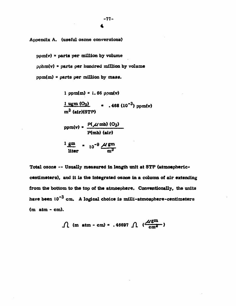
-77-

Appendix A. (useful ozone conversions)

ppm(v) = parts per million by volume

pphm(v) = parts per hundred million by volume

ppm(m) o parts per million by mass.

1 ppm(m) a 1. 66 ppm(v)

1 gm (0a) - . 468 (10- 3 ) ppm(v)m3 (air)(STP)

ppm(v) P(d mb) (03)

P(mb) (air)

1gm o.. gm

liter

Total ozone -- Usually measured in length unit at STP (atmospheric-

centimeters), and it is the integrated ozone in a column of air extending

from the bottom to the top of the atmosphere. Conventionally, the -units

have been 10- 3 cm. A logical choice is milli-atmosphere-centimeters

(m atm - cm).

S(m atm - cm) = . 4697 l ( - )

-78-

Appendix B.

The measurements of the halogens in this study have been supplied to

this author by his friend and colleague, Captian Ronald L. Lininger, a

fellow graduate student in the Department of Meteorology. They represent

a large part of his graduate thesis. His measurements have been collected

in the Cambridge-Boston complex using a Casella four stage cascade im-

pactor. The analysis for the halogens were conducted by pile neutron

activation. Since Captain Lininger's project began slightly earlier than

this study, there were no oione measurements for the first theree periods

or aerosol collection that totaled ten in all. The ozone meter operated

within a few yards of the cascade impactor intake orifice ouring the periods

of the remaining seven aerosol collections.

ACKNOWLEDGEMENTS

The author is extremely grateful to Professor Reginald E. Newell

for his advice, assistance, and enthusiasm in helping me to plan and

carry out this project. The author expresses his gratitude to Captain

fRonald L. Lininger for the use of his halogen measurements made at

the same time as part of this project and also for his support in the

many discussions concerning the study. Also, many thanks go to

Professor John W. Winchester and Dr. Robert A. Duce for their sug-

gestions on the instrumentation and for the use of the geochemistry

laboratory and equipment for the chemical phase and calibration of the

Mast ozone meter. The author wishes to thank Miss Ruth Benjamin

who has typed this manuscript.

Finally, the author is indebted to the Department of Defense,

which, through the Department of the Air Force has provided the

author's salary, tuition, and miscellaneous costs in making this edu-

cation and research possible; and also to the Office of Naval Research

whose futnds provided the author with the Mast ozone meter and recorder.

Lit