Embed Size (px)
Citation preview

FondazioneGiacomo Brodolini
IESS project is funded by the European Union Programme for Employment and Social Solidarity – PROGRESS (2007-2013). The information contained in this report reflects only the author’s view. The European Commission shall not be considered in any way responsible for any use that can be made of the information it contains.
Analysis report
IESS
Table of contents
Introduction 4
1. The data 5
2. Workers’ vulnerability in Italy: transitions among working statuses at a glance 10
Introduction 10
2.1 Transition matrixes 11
2.2 Downgrade risks and upgrade chances 18
2.3 Workers’ risks during the crisis 20
Conclusions 22
3. The new versions of T-DYMM 23
Introduction 23
3.1 Recent history of T-DYMM: the first release of the model 23
3.2 The new release of the model: from T-DYMM 1.0 to T-DYMM 2.0 25
3.2.1 The new simulation platform 25
3.2.2 The new structure of the model and the new characteristics of the modules 26
3.2.3 Demographic module 28
3.2.4 Labour market module 29
3.2.5 Pension module 30
3.2.6 Taxation module 37
References 39
4. The estimations employed in the modules 40
4.1 Estimations in the demographic module 42
4.1.1 Giving birth 42
4.1.2 Education 43
4.1.3 Marriage market 44
4.1.4 Divorce 46
4.2 Estimations in the labour market module 47
4.2.1 Transitions among employment states 47
4.2.2 Estimating gross earnings and months worked 55
4.3 Estimations in the pension module 60
References 62
5. Simulation results 63
5.1 Sample evolution at retirement 64
5.2 The evolution of adequacy indicators 68
5.3 The impact of private pension plans 71
References 74
6. Macro analysis on the effects of increasing the retirement age on GDP and on employment, especially of older workers 75
Introduction 75
6.1 Demographic developments in Europe 75
6.2 Short description of pension schemes in the EU 77
6.3 Labour force projections and participation rate: the deterministic approach of the 2015 Ageing Report 82
6.4 Pension reforms and participation rate: deterministic projections 85
6.5 A DSGE model for Italy: the FGB-MDL-MKIII 87
6.6 Other results based on DSGE models 88
References 89
Conclusions 90
iess Improving effectiveness in social security4
Introduction
The project “Improving effectiveness in social security” (henceforth IESS1), has been launched to provide innovative analytical tools in order to improve the effectiveness of public policy evaluation in the fields of labour market analysis, labour income distribution, public and private social security programs and retirement behaviour and, consequently, in order to help policy makers in their decisional process.
It largely benefitted from the work carried out in aa previous project “Innovative Datasets and Models for Improving Welfare Policies” which had as objective to fill the severe deficiency coming from current policy toolkit by developing: i) a dynamic microsimulation model (henceforth, DMSM) – called T-DYMM (Treasury Dynamic Microsimulation Model) – in order to simulate the evolution of cross-sectional sample representative of Italian population, with both individuals and households as units of analysis, and ii) a unique and innovative dataset – called “Administrative SILC”, henceforth AD-SILC – by matching longi-tudinal information coming from several administrative archives gathered by INPS (National Institute of Social Security) with survey data collected by ISTAT (National Institute of Statistics).
As a follow up of the previous project, the IESS aims at extending and improving the tools built in the recent past. In this respect, the project focuses, among other things, on two main activities: i) improving the dynamic micro-simulation model T-DYMM, and ii) updating and extending the innovative longitudi-nal dataset AD-SILC.
This analysis report has the objective to provide a detailed description of the state of art of the project. The following section presents the dataset resulting from the merge of statistical and administrative data, and explains how it is utilised for the various research purposes. Section 2 focuses on the main dynamic patterns of the Italian labour market in the period 2000-2011 as shown from administrative data, with particular focus on workers’ transitions and on the risks of unemployment during the current recession phase. The third section describes the structure and the characteristics of the microsimulation model T-DYMM in detail, highlighting the innovative features with respect to its old version. Section 4 is dedicated to the presentation of the estimations employed in the various modules contained in the model. Section 5 presents the main results of the microsimulations implemented so far in terms of trends of social se-curity aggregates, addressing adequacy concerns and analysing the impact of private pension schemes on the welfare system. Lastly, section 6 presents a survey of the literature on the impact of increased retirement ages over employment rates and GDP growth.
1 “Improving effectiveness in social security” (IESS), proposed by the Italian Ministry of Economy and Finance, Treasury Depart-ment (MEF DT), in partnership with Istituto Nazionale della Previdenza Sociale (INPS), Fondazione G. Brodolini (FGB) and Centre for Economic and Social Inclusion (CESI) and funded by the European Commission, DG Employment, Social Affairs and Inclusion.
iess Improving effectiveness in social security5
1. The data
Estimations and micro-simulations are based on an ad hoc longitudinal micro-data of the AD-SILC (e.g. administrative SILC) dataset. The dataset is particularly useful for analysing Italian labour market perfor-mance at individual level in the last decades focusing, in particular, on the dynamics of earnings distribu-tion, on individual transitions among the various working statuses and on the adequacy of contributions accumulated by cohorts of workers belonging to the new Notional Defined Contribution pension sche-me.
Moreover, the AD-SILC dataset is crucial for building the dynamic micro-simulation model T-DYMM, su-ited to evaluate the Italian pension system and fiscal policy changes. So far, the AD-SILC dataset has allowed to reconstruct the information relevant for the computation of future pension benefits of peo-ple applying both Defined Benefit (retributivo) and Notional Defined Contribution (contributivo) rules, in accordance with the legislation in force.
The AD-SILC dataset has been built by merging longitudinal data collected in several administrative ar-chives. To this aim, INPS archives2, regarding all individuals belonging to the specific group such as for instance, private employees or professionals, have been merged with the survey micro-data IT-SILC, the Italian version of the EU country-specific survey EU-SILC3. This means that AD-SILC links rich information about individuals’ social and demographic background, gathered in IT-SILC, with information on their working histories, collected in the administrative archives from the beginning of the individual working life (e.g. from the moment he/she starts belong to a specific group within the administrative archives) up until 2013/2014.
More in detail, considering the individuals sampled in any of the IT-SILC waves, INPS took their fiscal co-des (e.g. a unique key characterizing all residents in Italy) and drew out from its archives all the available records concerning those individuals. Once these records were drawn out, INPS blanked fiscal codes for privacy reasons, replacing them with an individual identification key. Hence, by means of the identifica-tion key, the administrative archives were merged in a single, very large administrative dataset and then linked to individuals surveyed by IT-SILC, provided they had any data related to them in the Register of Active Workers or in the Register of Retirees.
The completion of the merging procedure produces a panel AD-SILC which is very large over the retro-spective horizon (and in many cases also in projection) , where individuals’ data are recorded since their entry in the labour market up to 2013/2014. Clearly, AD-SILC is an unbalanced panel because, by defini-tion, individuals are followed for a different number of years.
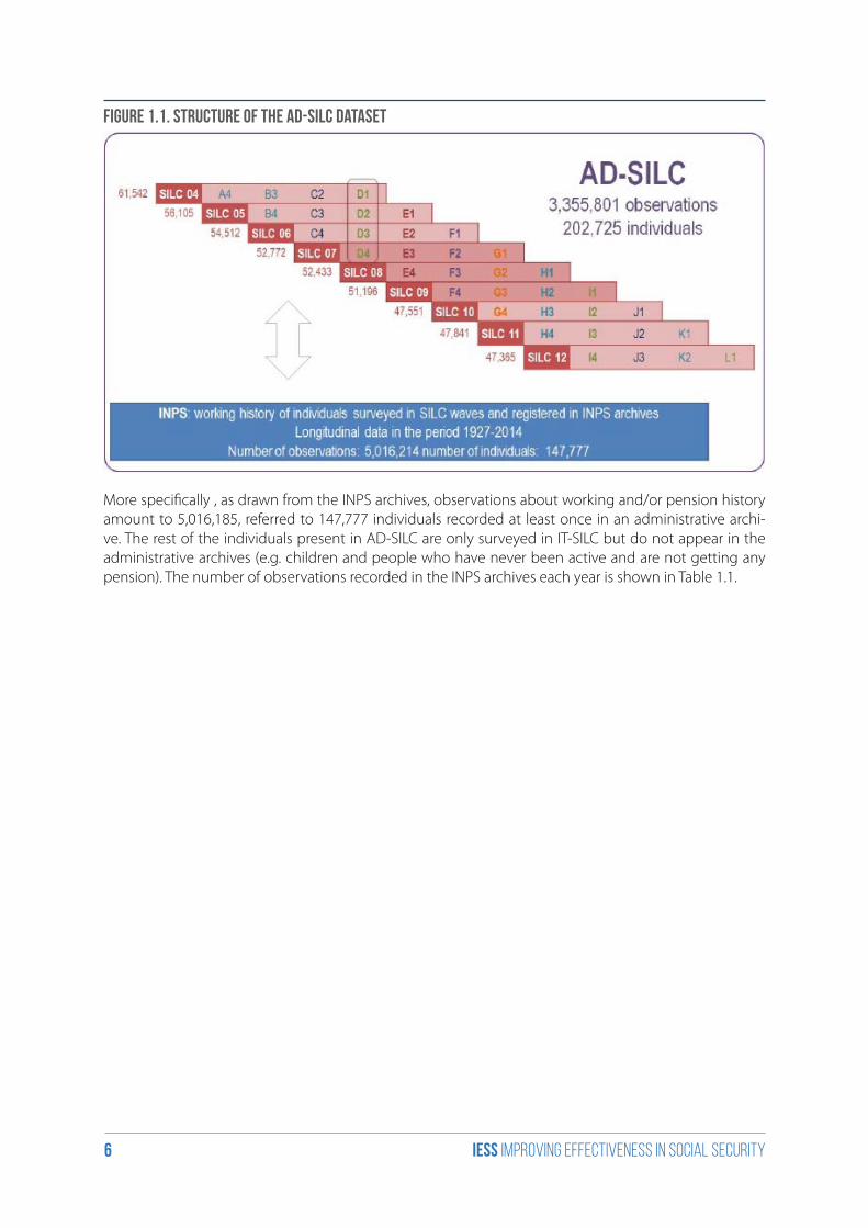
Figure 1.1 shows the design of AD-SILC, whose sample size amounts to 202,725 individuals correspon-ding to 3,355,801 annual observations.
2 INPS (National Institute of Social Security) provides information about active people (Register of Active Workers – EC_INPS) and about retired workers (Register of Retirees-PENSIONI).3 In the first version of AD-SILC developed for the first version of T-DYMM – only cross-sectional data of IT-SILC 2005 had been uti-lized, while eight more waves (data collected in IT-SILC from 2004 to 2012) have been added in the current version of the dataset.
iess Improving effectiveness in social security6
Figure 1.1. Structure of the AD-SILC dataset
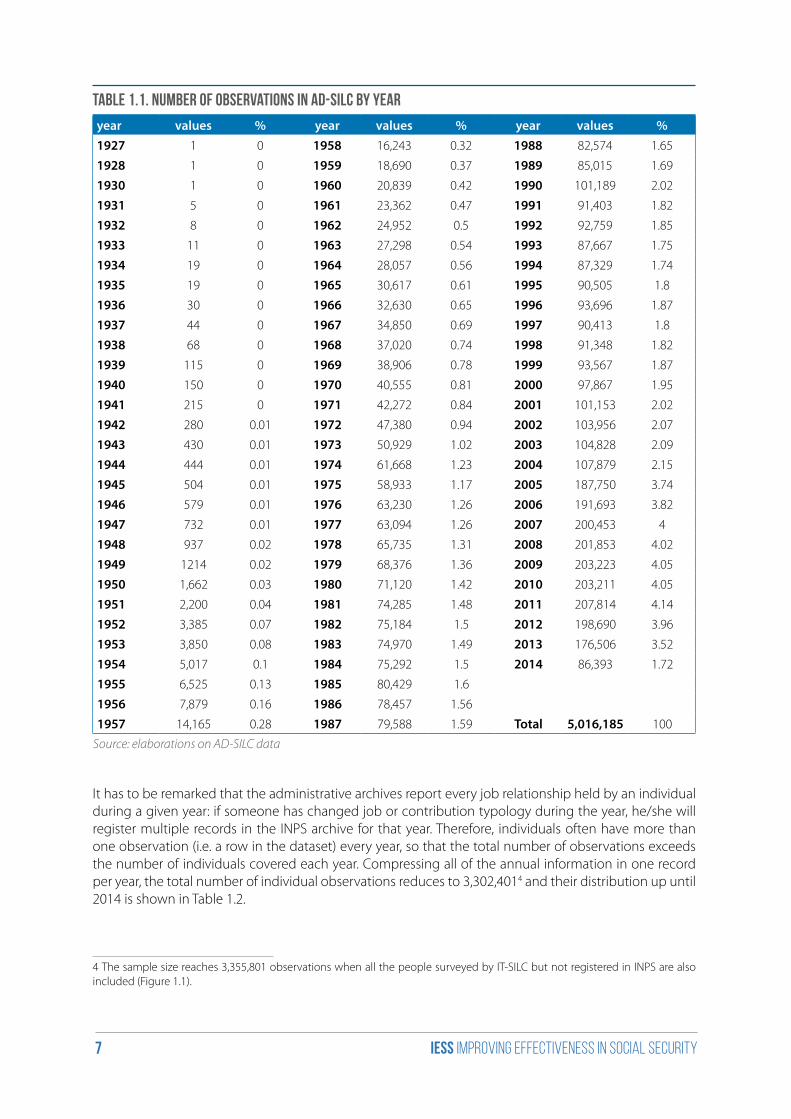
More specifically , as drawn from the INPS archives, observations about working and/or pension history amount to 5,016,185, referred to 147,777 individuals recorded at least once in an administrative archi-ve. The rest of the individuals present in AD-SILC are only surveyed in IT-SILC but do not appear in the administrative archives (e.g. children and people who have never been active and are not getting any pension). The number of observations recorded in the INPS archives each year is shown in Table 1.1.
iess Improving effectiveness in social security7
Table 1.1. Number of observations in AD-SILC by year
year values % year values % year values %1927 1 0 1958 16,243 0.32 1988 82,574 1.65
1928 1 0 1959 18,690 0.37 1989 85,015 1.69
1930 1 0 1960 20,839 0.42 1990 101,189 2.02
1931 5 0 1961 23,362 0.47 1991 91,403 1.82
1932 8 0 1962 24,952 0.5 1992 92,759 1.85
1933 11 0 1963 27,298 0.54 1993 87,667 1.75
1934 19 0 1964 28,057 0.56 1994 87,329 1.74
1935 19 0 1965 30,617 0.61 1995 90,505 1.8
1936 30 0 1966 32,630 0.65 1996 93,696 1.87
1937 44 0 1967 34,850 0.69 1997 90,413 1.8
1938 68 0 1968 37,020 0.74 1998 91,348 1.82
1939 115 0 1969 38,906 0.78 1999 93,567 1.87
1940 150 0 1970 40,555 0.81 2000 97,867 1.95
1941 215 0 1971 42,272 0.84 2001 101,153 2.02
1942 280 0.01 1972 47,380 0.94 2002 103,956 2.07
1943 430 0.01 1973 50,929 1.02 2003 104,828 2.09
1944 444 0.01 1974 61,668 1.23 2004 107,879 2.15
1945 504 0.01 1975 58,933 1.17 2005 187,750 3.74
1946 579 0.01 1976 63,230 1.26 2006 191,693 3.82
1947 732 0.01 1977 63,094 1.26 2007 200,453 4
1948 937 0.02 1978 65,735 1.31 2008 201,853 4.02
1949 1214 0.02 1979 68,376 1.36 2009 203,223 4.05
1950 1,662 0.03 1980 71,120 1.42 2010 203,211 4.05
1951 2,200 0.04 1981 74,285 1.48 2011 207,814 4.14
1952 3,385 0.07 1982 75,184 1.5 2012 198,690 3.96
1953 3,850 0.08 1983 74,970 1.49 2013 176,506 3.52
1954 5,017 0.1 1984 75,292 1.5 2014 86,393 1.72
1955 6,525 0.13 1985 80,429 1.6
1956 7,879 0.16 1986 78,457 1.56
1957 14,165 0.28 1987 79,588 1.59 Total 5,016,185 100
Source: elaborations on AD-SILC data
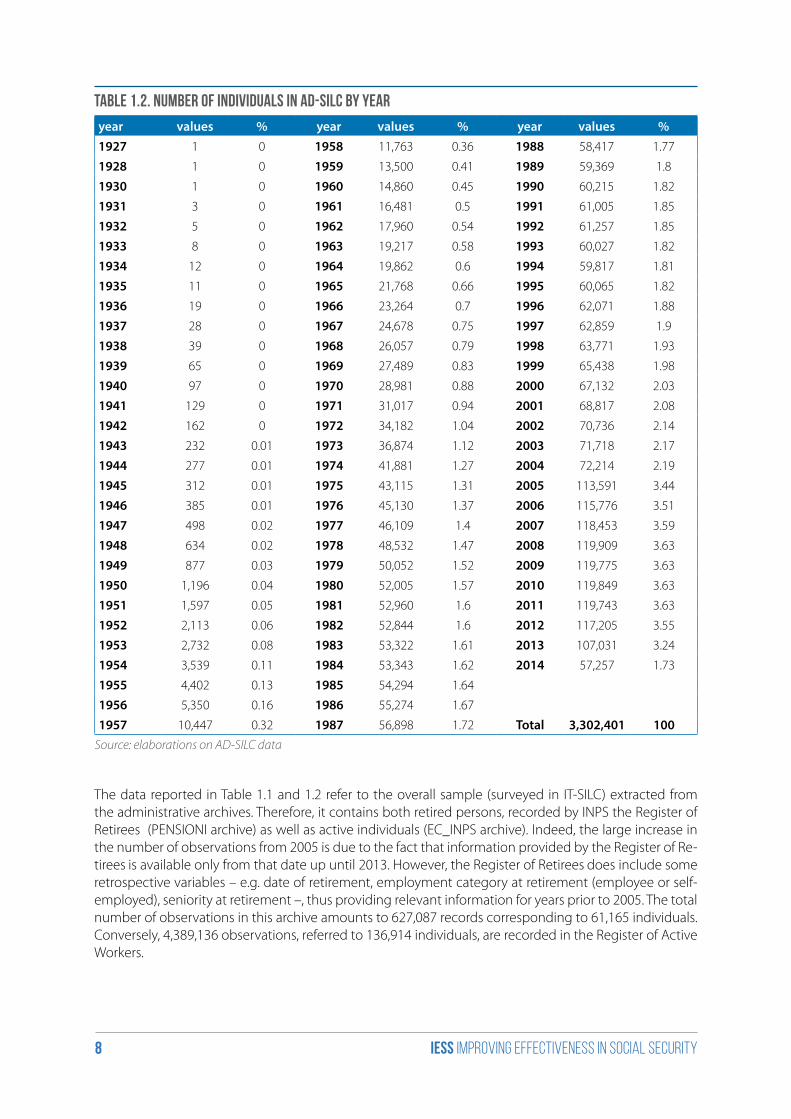
It has to be remarked that the administrative archives report every job relationship held by an individual during a given year: if someone has changed job or contribution typology during the year, he/she will register multiple records in the INPS archive for that year. Therefore, individuals often have more than one observation (i.e. a row in the dataset) every year, so that the total number of observations exceeds the number of individuals covered each year. Compressing all of the annual information in one record per year, the total number of individual observations reduces to 3,302,4014 and their distribution up until 2014 is shown in Table 1.2.
4 The sample size reaches 3,355,801 observations when all the people surveyed by IT-SILC but not registered in INPS are also included (Figure 1.1).
iess Improving effectiveness in social security8
Table 1.2. Number of individuals in AD-SILC by year
year values % year values % year values %1927 1 0 1958 11,763 0.36 1988 58,417 1.77
1928 1 0 1959 13,500 0.41 1989 59,369 1.8
1930 1 0 1960 14,860 0.45 1990 60,215 1.82
1931 3 0 1961 16,481 0.5 1991 61,005 1.85
1932 5 0 1962 17,960 0.54 1992 61,257 1.85
1933 8 0 1963 19,217 0.58 1993 60,027 1.82
1934 12 0 1964 19,862 0.6 1994 59,817 1.81
1935 11 0 1965 21,768 0.66 1995 60,065 1.82
1936 19 0 1966 23,264 0.7 1996 62,071 1.88
1937 28 0 1967 24,678 0.75 1997 62,859 1.9
1938 39 0 1968 26,057 0.79 1998 63,771 1.93
1939 65 0 1969 27,489 0.83 1999 65,438 1.98
1940 97 0 1970 28,981 0.88 2000 67,132 2.03
1941 129 0 1971 31,017 0.94 2001 68,817 2.08
1942 162 0 1972 34,182 1.04 2002 70,736 2.14
1943 232 0.01 1973 36,874 1.12 2003 71,718 2.17
1944 277 0.01 1974 41,881 1.27 2004 72,214 2.19
1945 312 0.01 1975 43,115 1.31 2005 113,591 3.44
1946 385 0.01 1976 45,130 1.37 2006 115,776 3.51
1947 498 0.02 1977 46,109 1.4 2007 118,453 3.59
1948 634 0.02 1978 48,532 1.47 2008 119,909 3.63
1949 877 0.03 1979 50,052 1.52 2009 119,775 3.63
1950 1,196 0.04 1980 52,005 1.57 2010 119,849 3.63
1951 1,597 0.05 1981 52,960 1.6 2011 119,743 3.63
1952 2,113 0.06 1982 52,844 1.6 2012 117,205 3.55
1953 2,732 0.08 1983 53,322 1.61 2013 107,031 3.24
1954 3,539 0.11 1984 53,343 1.62 2014 57,257 1.73
1955 4,402 0.13 1985 54,294 1.64
1956 5,350 0.16 1986 55,274 1.67
1957 10,447 0.32 1987 56,898 1.72 Total 3,302,401 100Source: elaborations on AD-SILC data
The data reported in Table 1.1 and 1.2 refer to the overall sample (surveyed in IT-SILC) extracted from the administrative archives. Therefore, it contains both retired persons, recorded by INPS the Register of Retirees (PENSIONI archive) as well as active individuals (EC_INPS archive). Indeed, the large increase in the number of observations from 2005 is due to the fact that information provided by the Register of Re-tirees is available only from that date up until 2013. However, the Register of Retirees does include some retrospective variables – e.g. date of retirement, employment category at retirement (employee or self-employed), seniority at retirement –, thus providing relevant information for years prior to 2005. The total number of observations in this archive amounts to 627,087 records corresponding to 61,165 individuals. Conversely, 4,389,136 observations, referred to 136,914 individuals, are recorded in the Register of Active Workers.
iess Improving effectiveness in social security9
It should be noted that most of the surveyed persons are present in the EC_INPS archive as they result active – or in any event not retired – by their last record in the administrative archives. However, because AD-SILC is mainly a retrospective panel database it provides the entire working history also for workers already in retirement; consequently, a significant number of individuals are present in both registers. Fi-nally, some individuals present in the Register of Retirees have never paid any contributions in their lives. These are generally people receiving invalidity or survivor’s pensions. In particular, 10,854 individuals do not appear in the Register of Active Workers for the above-mentioned reasons, almost 70 percent of whom are women.
For the purposes of the IESS project, we employ the AD-SILC dataset in various ways. In particular, we can identify three main applications of AD-SILC: i) analyses of the Italian labour market dynamics in the past decades up until now; ii) estimation of the parameters needed for the different modules that constitute the T-DYMM model; iii) micro-simulations to evaluate the Italian pension system and fiscal policy chan-ges.
In each of these three fields, a specific configuration of the dataset has been carried out. It has to be re-minded that various records per year are often present in the administrative archives, but all of the listed uses we have employed annual observations. For this reason, we had to aggregate data in order to have one single record including all relevant information relative to that year. For instance, for the scopes in i), the data are annualised considering working conditions occurred at the end of the year5. For the analyses comprised in point ii), data have been annualised aggregating the single observations registered in a given year into one single annual record based on the prevalent job a worker held in that year, while still preserving some important information like the total annual amount of weeks of contribution, total ear-nings, etc. Therefore, we do not refer to a particular time (month, week or day) of the year but we retrace the predominant condition of the individual in a given year.
Furthermore, for the purposes of i) and ii) we make use of the entire dataset (i.e. including all SILC waves, from 2004 to 2012), while as starting population for our micro-simulations (point iii) we only use one part of the dataset – the subsample referred to the IT-SILC wave 2011 and merged with the INPS data. By this way, the year 2011 represents the starting point of the simulation , with a sample which is representative of the Italian population in that year. The dataset used for this purpose is cross-sectional, yet integrated with retrospective information about working conditions, acquired work experience, total number of years of contribution, etc.
Two reasons have guided the choice of 2011 as baseline year for T-DYMM simulations. First, the informa-tion on public workers in the INPS archives is not accountable after 2011. In addition, 2011 was the year of the last major reform of the pension system in Italy (the so-called “Fornero Reform”). By choosing 2011 as baseline year, we allow ourselves the possibility to implement scenarios where the previous legislation is kept in force.
5 If an individual is not present in the register for most of the time in a given year, but recorded as an employee in December, then the individual will be considered as an employee for that year. Conversely, if an individual has worked and paid contribu-tions for several months during a year but is not recorded in December, then he/she will result not employed that year.
iess Improving effectiveness in social security10
2. Workers’ vulnerability in Italy: transitions among working statuses at a glance
Introduction
The analysis of workers’ vulnerability in a multi-year period requires a deep longitudinal investigation of individuals’ movements across the various working conditions and a detailed exam of the relationship between contractual arrangements and individual career prospects. In particular, temporary and perma-nent workers’ prospects can be mainly assessed in terms of mobility towards better or worse working statuses. For instance, low transition rates between fixed-term and permanent positions could imply entrapment in insecure jobs and poor career prospects for those who do not succeed in getting into stable employment soon.
Since the ‘90s, the Italian labour market has experienced several legislative interventions aimed at intro-ducing various flexible contractual arrangements. It is partly because of these legislative interventions that the labour market segmentation between temporary and permanent workers has been increasing in Italy over the last years. In order to properly analyse labour market segmentation and the extent of the vulnerability of the working condition in the Italian labour market, it is then crucial to investigate workers’ transitions among different statuses. Labour market segmentation and the related problems of preca-riousness and insecurity are recorded when the most disadvantaged condition (being a worker with a temporary/atypical contract) is not a transitory phenomenon (i.e. in the stage of entry to or exit from the labour market), but rather becomes a permanent status. Likewise, workers’ vulnerability could be observed also when a large share of the supposedly “guaranteed” individuals – i.e. those working through open-ended arrangements – experience a worsening of their status.
Actually, investigating workers mobility in the medium run in the Italian case is of the outmost importan-ce also in order to inquire the possible future effects of the recently introduced labour market reform (the so-called Jobs Act) that has modified the contractual arrangement for those who will be hired with an open-ended contract since March 2015 introducing open-ended contracts with increasing protection according to tenure.
Assessing individual transitions among different working statuses requires the availability of a longitudi-nal micro dataset – i.e. the same individual has to be observed for many years – where detailed informa-tion about socio-economic characteristics of the interviewed people are included. Therefore, the AD-SILC dataset (i.e. the panel dataset built by merging the IT-SILC waves with the information collected in INPS’ administrative archives) is very well suited to the aim of studying in-depth short, medium and long-term individual transitions among different working statuses, also comparing the working histories of indivi-duals with different characteristics (e.g. gender and educational attainment).
Observing individual transitions among the various employment statuses in a decade is crucial for as-sessing the extent of workers’ vulnerability in Italy – over aggregate indexes of precariousness (e.g., the share of atypical workers in a given year) – and for trying to answer to several research questions, as the following:

iess Improving effectiveness in social security11
• Is there an actual dual labour market?
• Does a sort of “liquidity” of the labour market emerge, also before the crisis?
• Are temporary contracts a trap or a stepping stone?
• Do permanent contracts and stabilization cover individuals against risks?
• Is it enough to focus on being hired through an open-ended arrangement?
• Are only some groups of individuals exposed to risks?
In the following sections we provide useful evidences in order to try to answer to these questions, show-ing the individual transition matrixes among the various working statuses in a 12-years period (i.e. in the period 2000-2011; section 2.2), then computing downgrade risks and upgrade chances for those working, respectively, with permanent and temporary arrangements (section 2.3). Lastly, we show some evidences about the risks of being fired during the current recession phase (section 2.4). Section 2.5 concludes.
2.1 Transition matrixes
In order to answer the questions listed in the introduction, as a first set of analyses, we follow the indi-viduals that were working in 2000 up to 2011 and compute the transitions matrixes from the working status in 2000 to the statuses achieved in the following years. We exclude from the analyses the older workers, thus we restrain our subsample to those born since 1950. Furthermore, we exclude the few in-dividuals who retired or died during the observation period.
We define yearly individual working statuses as the status held by the individual at the end of a given year (i.e. at December). We identify 7 possible working statuses: i) private employee with an open-ended arrangement; ii) private employee with a fixed-term arrangement; iii) public employee with an open-ended arrangement; iv) public employee with a fixed-term arrangement; v) atypical worker (where we include those working with the so-called “parasubordinate” arrangements and enrolled to the Gestione Separata, the pension fund for parasubordinate collaborators and self-employed not enrolled in other types of pension funds); vi) self-employed enrolled in INPS (craftsmen, shopkeepers and self-employed farmers); vii) professionals (e.g. lawyers, architects, i.e. professional workers who are enrolled in pension funds managed by their professional association). In addition, as destinations, we consider two further statuses: viii) unemployed (i.e. those working during a year, but not working at the end of the year); ix) inactive (those not working during a whole year). Note also that periods spent receiving allowances for maternity, sickness or temporary layoff (Cassa Integrazione) are considered as an employment period, because the contractual arrangement does not interrupt when these contingencies occur.
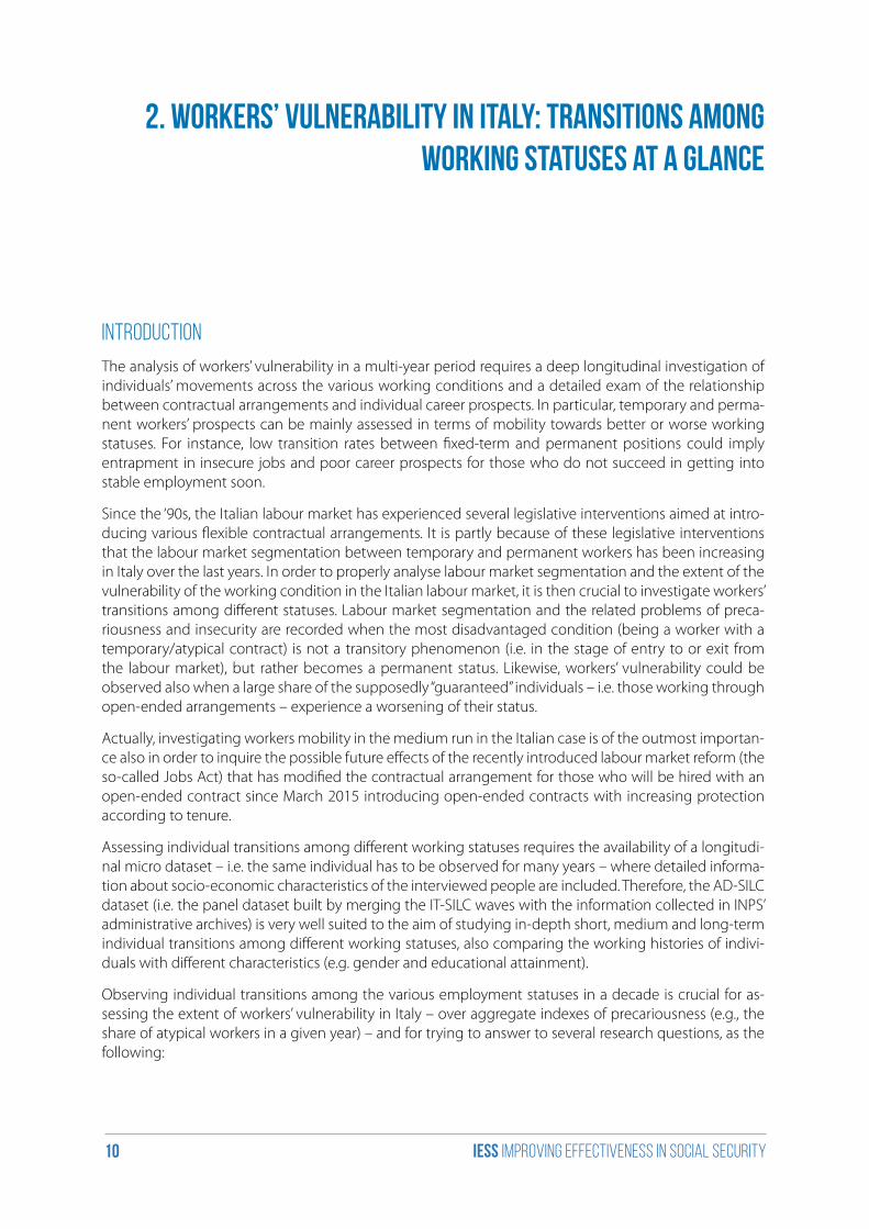
However, before discussing the main results highlighted by the transition matrixes, it is interesting to present the distribution of the workforce by type of employment, gender and educational attainment in 2000 and 2011. About 60% of workers had a private employment arrangement in 2000 and, among these, 12.7% had a fixed-term contract (Figure 2.1). The share of public employees amounted to 17.1% (the share of temporary workers in public employment was 1.8%), while the shares of atypical workers (i.e. those enrolled to the Gestione Separata), “pure” self-employed and professionals were, respectively, 3.9%, 16.0% and 2.5%.
Among females, public employment is relatively more diffused, but so are temporary contracts, for what concerns both fixed-term employment and atypical contracts (respectively, 9.2% and 4.3 among fema-les, versus 7.1% and 3.6% among males). The share of males working as self-employed or professionals is much higher than the share of females performing these types of jobs (respectively, 21.5% versus 14.5%).
iess Improving effectiveness in social security12
Figure 2.1. Distribution by employment status of the workforce in 2000, by gender and education
52,7% 55,1%49,4%
59,2%54,2%
30,2%
7,7%7,1%
8,6%
10,1%
6,6%
5,3%
16,8% 12,6% 22,5%7,6%
18,4%
35,4%
0,3%0,1%
0,6% 0,1% 0,3%
1,0%
3,9%3,6%
4,3%1,8% 4,0%
9,2%
16,0% 18,5%12,5%
21,1% 15,2%
5,3%
2,5% 3,0% 2,0% 0,1% 1,3%
13,5%
0%
10%
20%
30%
40%
50%
60%
70%
80%
90%
100%
Male Female At most low. Sec. Upper sec. Tertiary
Total Gender Education
Perm. pr. emp. F.T. pr. emp. Perm. pub. emp. F.T. pub. emp. Gestione Separata Self-employed Professionals
Source: elaborations on AD-SILC data
Clear differences emerge when we distinguish individuals by education. In particular, tertiary graduates (that are still a minority in the Italian workforce) are more likely to work as public employees and, as expected, as professionals (the degree often being a prerequisite for performing professional activities). Conversely, the shares of those working as employees or self-employed are much higher among less educated workers. Interestingly, atypical arrangements are more diffused among tertiary graduates than among the low skilled (9.2% of tertiary graduates had an atypical arrangement in 2000, while these sha-res were 1.8% and 4.0% among those who have achieved, respectively, at most a lower secondary degree and an upper secondary degree).
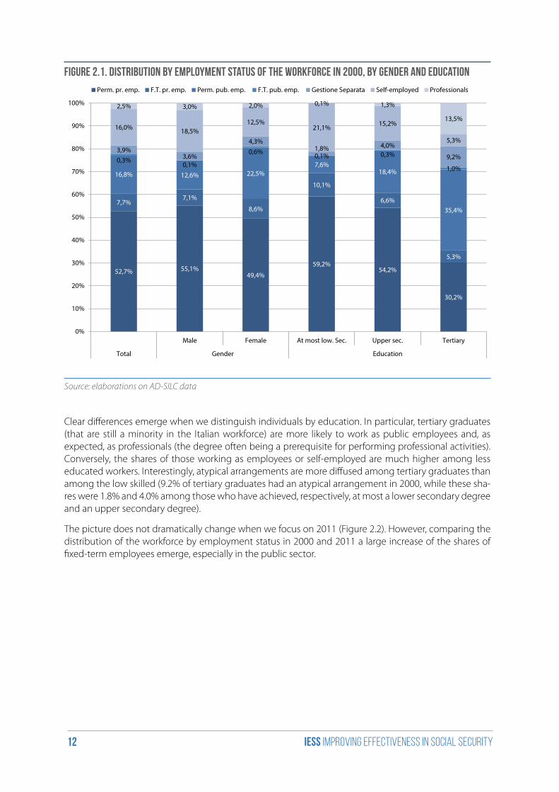
The picture does not dramatically change when we focus on 2011 (Figure 2.2). However, comparing the distribution of the workforce by employment status in 2000 and 2011 a large increase of the shares of fixed-term employees emerge, especially in the public sector.
iess Improving effectiveness in social security13
Figure 2.2. Distribution by employment status of the workforce in 2011, by gender and education
51,1% 52,8%48,9%
57,0% 53,3%
33,6%
8,7% 8,0%9,5%
13,0%
7,3%
4,0%
15,8% 12,1% 20,3%
7,8%
16,2%
29,5%
1,6%0,7%
2,7%0,5% 1,4%
4,3%
5,2%5,2%
5,3%2,8% 5,4%
9,0%
14,3%17,4%
10,4% 18,7% 14,7%
5,4%
3,4% 3,8% 2,9% 0,3% 1,7%
14,1%
0%
10%
20%
30%
40%
50%
60%
70%
80%
90%
100%
Male Female At most low. Sec. Upper sec. Tertiary
Total Gender Education
Perm. pr. emp. F.T. pr. emp. Perm. pub. emp. F.T. pub. emp. Gestione Separata Self-employed Professionals
Source: elaborations on AD-SILC data
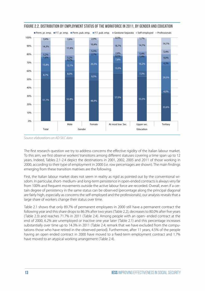
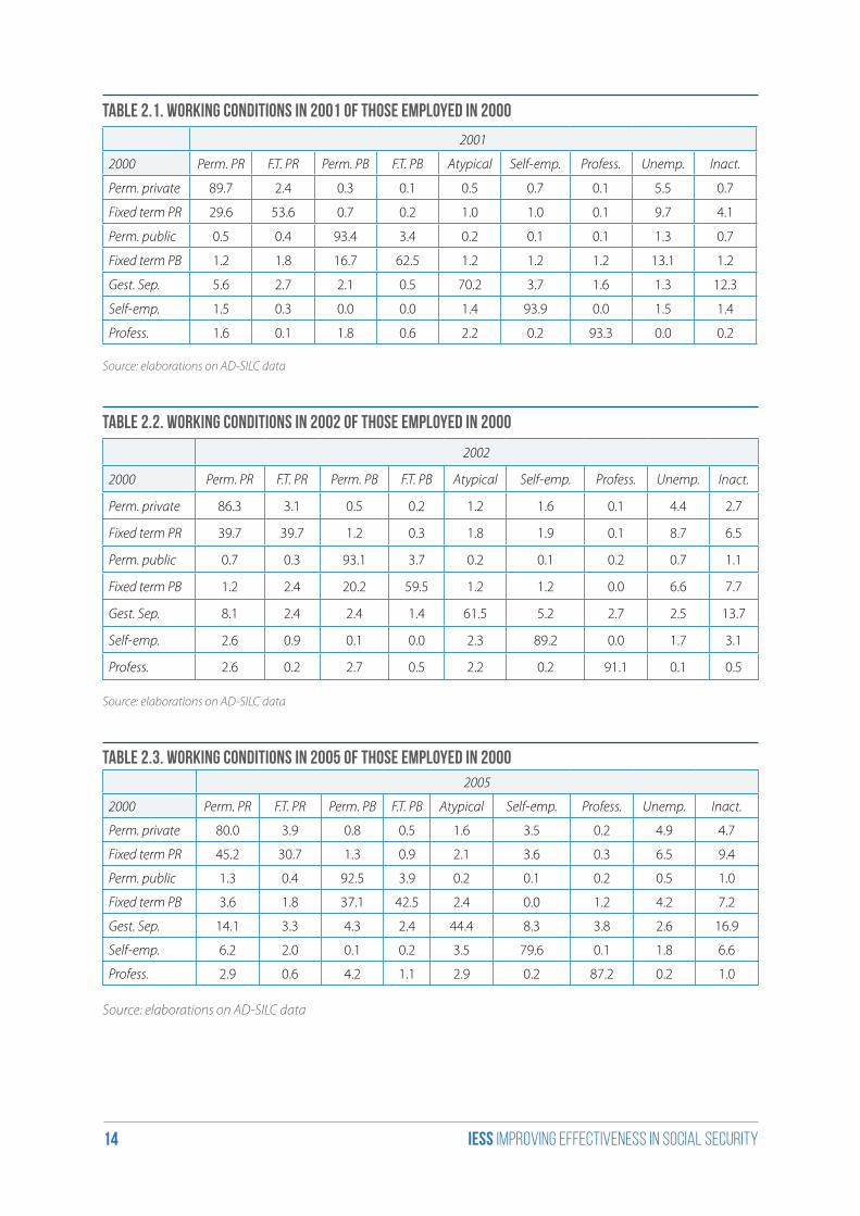
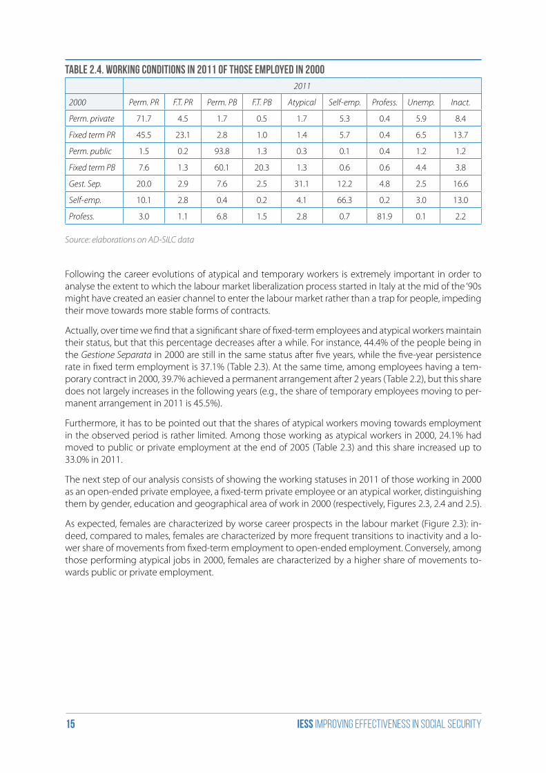
The first research question we try to address concerns the effective rigidity of the Italian labour market. To this aim, we first observe workers’ transitions among different statuses covering a time span up to 12 years. Indeed, Tables 2.1-2.4 depict the destinations in 2001, 2002, 2005 and 2011 of those working in 2000, according to their type of employment in 2000 (i.e. row percentages are shown). The main findings emerging from these transition matrixes are the following.
First, the Italian labour market does not seem in reality as rigid as pointed out by the conventional wi-sdom. In particular, short- medium- and long-term persistence in open-ended contracts is always very far from 100% and frequent movements outside the active labour force are recorded. Overall, even if a cer-tain degree of persistency in the same status can be observed (percentage along the principal diagonal are fairly high, especially as concerns the self-employed and the professionals), our analysis reveals that a large share of workers change their status over time.
Table 2.1 shows that only 89.7% of permanent employees in 2000 still have a permanent contract the following year and this share drops to 86.3% after two years (Table 2.2), decreases to 80.0% after five years (Table 2.3) and reaches 71.7% in 2011 (Table 2.4). Among people with an open- ended contract at the end of 2000, 6.2% are unemployed or inactive one year later (Table 2.1) and this percentage increases substantially over time up to 14.3% in 2011 (Table 2.4; remark that we have excluded from the compu-tations those who have retired in the observed period). Furthermore, after 11 years, 4.5% of the people having an open ended contract in 2000 have moved to a fixed-term employment contract and 1.7% have moved to an atypical working arrangement (Table 2.4).
iess Improving effectiveness in social security14
Table 2.1. Working conditions in 2001 of those employed in 2000
2001
2000 Perm. PR F.T. PR Perm. PB F.T. PB Atypical Self-emp. Profess. Unemp. Inact.
Perm. private 89.7 2.4 0.3 0.1 0.5 0.7 0.1 5.5 0.7
Fixed term PR 29.6 53.6 0.7 0.2 1.0 1.0 0.1 9.7 4.1
Perm. public 0.5 0.4 93.4 3.4 0.2 0.1 0.1 1.3 0.7
Fixed term PB 1.2 1.8 16.7 62.5 1.2 1.2 1.2 13.1 1.2
Gest. Sep. 5.6 2.7 2.1 0.5 70.2 3.7 1.6 1.3 12.3
Self-emp. 1.5 0.3 0.0 0.0 1.4 93.9 0.0 1.5 1.4
Profess. 1.6 0.1 1.8 0.6 2.2 0.2 93.3 0.0 0.2
Source: elaborations on AD-SILC data
Table 2.2. Working conditions in 2002 of those employed in 2000
2002
2000 Perm. PR F.T. PR Perm. PB F.T. PB Atypical Self-emp. Profess. Unemp. Inact.
Perm. private 86.3 3.1 0.5 0.2 1.2 1.6 0.1 4.4 2.7
Fixed term PR 39.7 39.7 1.2 0.3 1.8 1.9 0.1 8.7 6.5
Perm. public 0.7 0.3 93.1 3.7 0.2 0.1 0.2 0.7 1.1
Fixed term PB 1.2 2.4 20.2 59.5 1.2 1.2 0.0 6.6 7.7
Gest. Sep. 8.1 2.4 2.4 1.4 61.5 5.2 2.7 2.5 13.7
Self-emp. 2.6 0.9 0.1 0.0 2.3 89.2 0.0 1.7 3.1
Profess. 2.6 0.2 2.7 0.5 2.2 0.2 91.1 0.1 0.5
Source: elaborations on AD-SILC data
Table 2.3. Working conditions in 2005 of those employed in 20002005
2000 Perm. PR F.T. PR Perm. PB F.T. PB Atypical Self-emp. Profess. Unemp. Inact.
Perm. private 80.0 3.9 0.8 0.5 1.6 3.5 0.2 4.9 4.7
Fixed term PR 45.2 30.7 1.3 0.9 2.1 3.6 0.3 6.5 9.4
Perm. public 1.3 0.4 92.5 3.9 0.2 0.1 0.2 0.5 1.0
Fixed term PB 3.6 1.8 37.1 42.5 2.4 0.0 1.2 4.2 7.2
Gest. Sep. 14.1 3.3 4.3 2.4 44.4 8.3 3.8 2.6 16.9
Self-emp. 6.2 2.0 0.1 0.2 3.5 79.6 0.1 1.8 6.6
Profess. 2.9 0.6 4.2 1.1 2.9 0.2 87.2 0.2 1.0
Source: elaborations on AD-SILC data
iess Improving effectiveness in social security15
Table 2.4. Working conditions in 2011 of those employed in 20002011
2000 Perm. PR F.T. PR Perm. PB F.T. PB Atypical Self-emp. Profess. Unemp. Inact.
Perm. private 71.7 4.5 1.7 0.5 1.7 5.3 0.4 5.9 8.4
Fixed term PR 45.5 23.1 2.8 1.0 1.4 5.7 0.4 6.5 13.7
Perm. public 1.5 0.2 93.8 1.3 0.3 0.1 0.4 1.2 1.2
Fixed term PB 7.6 1.3 60.1 20.3 1.3 0.6 0.6 4.4 3.8
Gest. Sep. 20.0 2.9 7.6 2.5 31.1 12.2 4.8 2.5 16.6
Self-emp. 10.1 2.8 0.4 0.2 4.1 66.3 0.2 3.0 13.0
Profess. 3.0 1.1 6.8 1.5 2.8 0.7 81.9 0.1 2.2
Source: elaborations on AD-SILC data
Following the career evolutions of atypical and temporary workers is extremely important in order to analyse the extent to which the labour market liberalization process started in Italy at the mid of the ‘90s might have created an easier channel to enter the labour market rather than a trap for people, impeding their move towards more stable forms of contracts.
Actually, over time we find that a significant share of fixed-term employees and atypical workers maintain their status, but that this percentage decreases after a while. For instance, 44.4% of the people being in the Gestione Separata in 2000 are still in the same status after five years, while the five-year persistence rate in fixed term employment is 37.1% (Table 2.3). At the same time, among employees having a tem-porary contract in 2000, 39.7% achieved a permanent arrangement after 2 years (Table 2.2), but this share does not largely increases in the following years (e.g., the share of temporary employees moving to per-manent arrangement in 2011 is 45.5%).
Furthermore, it has to be pointed out that the shares of atypical workers moving towards employment in the observed period is rather limited. Among those working as atypical workers in 2000, 24.1% had moved to public or private employment at the end of 2005 (Table 2.3) and this share increased up to 33.0% in 2011.
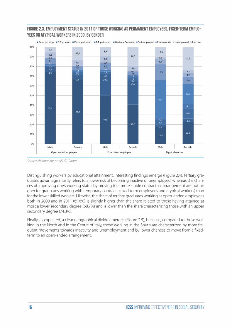
The next step of our analysis consists of showing the working statuses in 2011 of those working in 2000 as an open-ended private employee, a fixed-term private employee or an atypical worker, distinguishing them by gender, education and geographical area of work in 2000 (respectively, Figures 2.3, 2.4 and 2.5).
As expected, females are characterized by worse career prospects in the labour market (Figure 2.3): in-deed, compared to males, females are characterized by more frequent transitions to inactivity and a lo-wer share of movements from fixed-term employment to open-ended employment. Conversely, among those performing atypical jobs in 2000, females are characterized by a higher share of movements to-wards public or private employment.
iess Improving effectiveness in social security16
Figure 2.3. Employment status in 2011 of those working as permanent employees, fixed-term emplo-yees or atypical workers in 2000, by gender
75,0
66,8
49,8
40,6
17,422,8
4,5
4,6 22,2
24,2
2,3
3,4
1,1
2,5 2,4
3,2
4,9
10,6
0,2
0,9 0,5
1,6
1,0
4,1
1,7 1,8 1,6
1,2
40,3
20,8
6,1
4,1 7,2
3,9 16,3
7,6
0,4
0,40,4
0,3
5,6
3,9
5,8
6,07,0
5,9
1,7
3,3
5,3
13,08,9
19,0
10,4
23,5
0%
10%
20%
30%
40%
50%
60%
70%
80%
90%
100%
Male Female Male Female Male Female
Open ended employee Fixed term employee Atypical worker
Perm. pr. emp. F.T. pr. emp. Perm. pub. emp. F.T. pub. emp. Gestione Separata Self-employed Professionals Unemployed Inactive
Source: elaborations on AD-SILC data
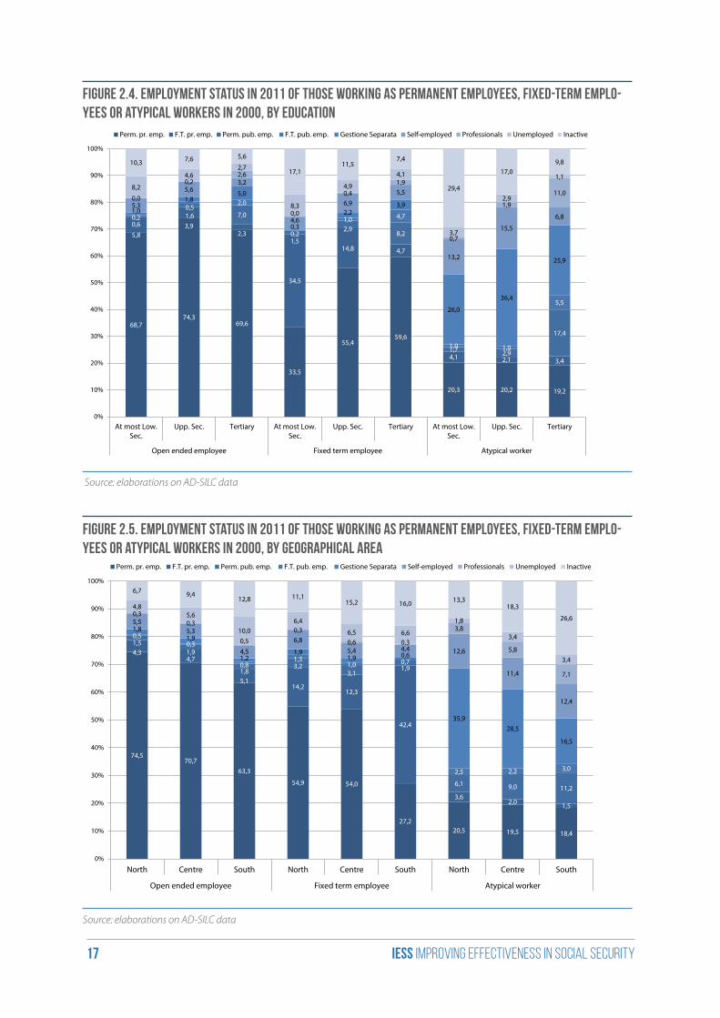
Distinguishing workers by educational attainment, interesting findings emerge (Figure 2.4). Tertiary gra-duates’ advantage mostly refers to a lower risk of becoming inactive or unemployed, whereas the chan-ces of improving one’s working status by moving to a more stable contractual arrangement are not hi-gher for graduates working with temporary contracts (fixed-term employees and atypical workers) than for the lower skilled workers. Likewise, the share of tertiary graduates working as open-ended employees both in 2000 and in 2011 (69.6%) is slightly higher than the share related to those having attained at most a lower secondary degree (68.7%) and is lower than the share characterizing those with an upper secondary degree (74.3%).
Finally, as expected, a clear geographical divide emerges (Figure 2.5), because, compared to those wor-king in the North and in the Centre of Italy, those working in the South are characterized by more fre-quent movements towards inactivity and unemployment and by lower chances to move from a fixed-term to an open-ended arrangement.
iess Improving effectiveness in social security17
Figure 2.4. Employment status in 2011 of those working as permanent employees, fixed-term emplo-yees or atypical workers in 2000, by education
68,774,3
69,6
33,5
55,459,6
20,3 20,2 19,2
5,83,9
2,3
34,5
14,8 4,7
4,1 2,1 3,4
0,61,6 7,0
1,5
2,98,2
1,7 2,9
17,4
0,20,5
2,0
0,2
1,0 4,7
1,0 1,0
5,5
1,0
1,85,0
0,3
2,23,9
26,0
36,4
25,9
5,3
5,63,2
4,6
6,9
5,5
13,2
15,5
6,8
0,0
0,22,6
0,0
0,4
1,9
0,7
1,9
11,08,2
4,62,7
8,3
4,9
4,1
3,7
2,9
1,1
10,3 7,6 5,6
17,111,5
7,4
29,4
17,09,8
0%
10%
20%
30%
40%
50%
60%
70%
80%
90%
100%
At most Low.Sec.
Upp. Sec. Tertiary At most Low.Sec.
Upp. Sec. Tertiary At most Low.Sec.
Upp. Sec. Tertiary
Open ended employee Fixed term employee Atypical worker
Perm. pr. emp. F.T. pr. emp. Perm. pub. emp. F.T. pub. emp. Gestione Separata Self-employed Professionals Unemployed Inactive
Source: elaborations on AD-SILC data
Figure 2.5. Employment status in 2011 of those working as permanent employees, fixed-term emplo-yees or atypical workers in 2000, by geographical area
74,570,7
63,3
54,9 54,0
27,220,5 19,5 18,4
4,34,7
5,114,2
12,3
42,4
3,62,0 1,5
1,51,9
1,83,2
3,11,9
6,1 9,0 11,2
0,50,3
0,81,3
1,0 0,7
2,5 2,2 3,0
1,81,9
1,21,9
1,9 0,6
35,928,5
16,5
5,55,3
4,5
6,8
5,4 4,4 12,6
11,4
12,4
0,30,3
0,5
0,3
0,6 0,3
3,8
5,8
7,1
4,85,6
10,06,4
6,5 6,6
1,8
3,4
3,4
6,7 9,412,8 11,1
15,2 16,0 13,318,3
26,6
0%
10%
20%
30%
40%
50%
60%
70%
80%
90%
100%
North Centre South North Centre South North Centre South
Open ended employee Fixed term employee Atypical worker
Perm. pr. emp. F.T. pr. emp. Perm. pub. emp. F.T. pub. emp. Gestione Separata Self-employed Professionals Unemployed Inactive
Source: elaborations on AD-SILC data
iess Improving effectiveness in social security18
2.2 Downgrade risks and upgrade chances
The matrixes depicted so far show “point to point” transitions, because they display individual move-ments in two specific points of time without informing, however, about what happens during the obser-ved period (for instance, observing transitions in the couple of years 2000 and 2005 does not inform us about individual movements in 2001, 2002, 2003 and 2004).
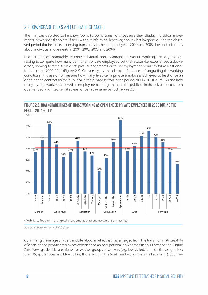
In order to more thoroughly describe individual mobility among the various working statuses, it is inte-resting to compute how many permanent private employees lost their status (i.e. experienced a down-grade, moving to fixed term or atypical arrangements or to unemployment or inactivity) at least once in the period 2000-2011 (Figure 2.6). Conversely, as an indicator of chances of upgrading the working conditions, it is useful to measure how many fixed-term private employees achieved at least once an open-ended contract (in the public or in the private sector) in the period 2000-2011 (Figure 2.7) and how many atypical workers achieved an employment arrangement (in the public or in the private sector, both open-ended and fixed term) at least once in the same period (Figure 2.8).
Figure 2.6. Downgrade risks of those working as open-ended private employees in 2000 during the period 2001-2011a
37%
48%
62%
44%
33%
37%
47%
38%
34%
20%
32%
46%
65%
38%
42%
51%
56%
50%
46%
37%
26%
0%
10%
20%
30%
40%
50%
60%
70%
Mal
es
Fem
ales
15-2
4
25-3
4
35-4
4
45-5
0
Low
. Sec
.
Upp
. Sec
.
Tert
iary
Man
ager
Whi
te-c
olla
r
Blue
-col
lar
App
rent
ices
Nor
th
Cent
re
Sout
h
1-5
6-15
16-4
9
50-2
49
>=25
0
Gender Age group Education Occupation Area Firm size
a Mobility to fixed-term or atypical arrangements or to unemployment or inactivity
Source: elaborations on AD-SILC data
Confirming the image of a very mobile labour market that has emerged from the transition matrixes, 41% of open-ended private employees experienced an occupational downgrade in an 11-year period (Figure 2.6). Downgrade risks are higher for weaker groups of workers (e.g. low skilled, females, those aged less than 35, apprentices and blue collars, those living in the South and working in small size firms), but inse-
iess Improving effectiveness in social security19
curities emerge also among the most advantaged groups (i.e. among tertiary graduates, those living in the North and working in large enterprises). In particular, no significant differences in workers’ risks emer-ge among permanent employees hired in firms whose size is around 15 employees, i.e. the threshold over which the reinstatement of employees at the job place in case of unfair dismissal was guaranteed before the introduction of the Jobs Act reform in March 2015.
Figure 2.7. Upgrade chances of those working as fixed-term private employees in 2000 during the period 2001-2011a
72,4%
61,5%
81,9%
75,6%
48,9%
33,3%
53,9%
79,0%
83,8%
91,9%
60,1% 61,5%
80,3% 80,0%
41,9%
0,0%
10,0%
20,0%
30,0%
40,0%
50,0%
60,0%
70,0%
80,0%
90,0%
100,0%
Mal
es
Fem
ales
15-2
4
25-3
4
35-4
4
45-5
0
Low
. Sec
.
Upp
. Sec
.
Tert
iary
Whi
te-c
olla
r
Blue
-col
lar
App
rent
ices
Nor
th
Cent
re
Sout
h
Gender Age group Education Occupation Area
a Mobility to open-ended private or public employment
Source: elaborations on AD-SILC data
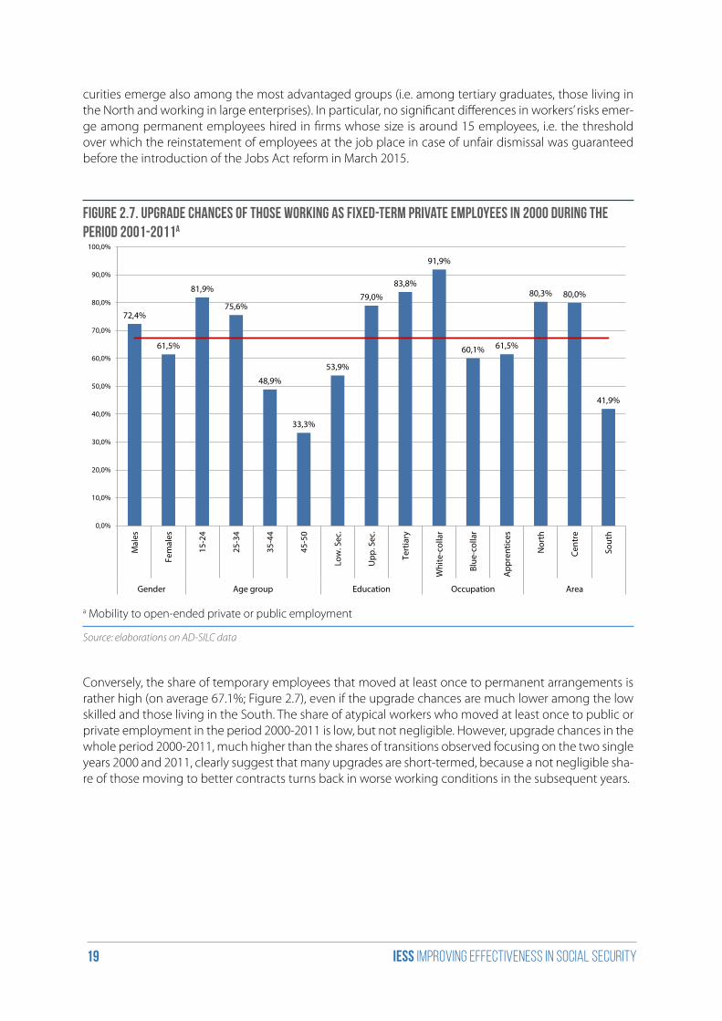
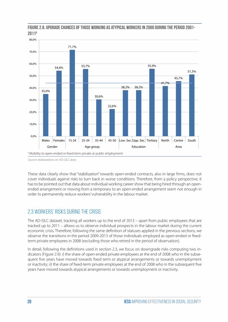
Conversely, the share of temporary employees that moved at least once to permanent arrangements is rather high (on average 67.1%; Figure 2.7), even if the upgrade chances are much lower among the low skilled and those living in the South. The share of atypical workers who moved at least once to public or private employment in the period 2000-2011 is low, but not negligible. However, upgrade chances in the whole period 2000-2011, much higher than the shares of transitions observed focusing on the two single years 2000 and 2011, clearly suggest that many upgrades are short-termed, because a not negligible sha-re of those moving to better contracts turns back in worse working conditions in the subsequent years.
iess Improving effectiveness in social security20
Figure 2.8. Upgrade chances of those working as atypical workers in 2000 during the period 2001-2011a
35,0%
54,4%
71,7%
55,7%
30,6%
22,6%
38,2% 38,2%
55,9%
41,7%45,7%
51,3%
0,0%
10,0%
20,0%
30,0%
40,0%
50,0%
60,0%
70,0%
80,0%
Males Females 15-24 25-34 35-44 45-50 Low. Sec. Upp. Sec. Tertiary North Centre South
Gender Age group Education Area
a Mobility to open-ended or fixed-term private or public employment
Source: elaborations on AD-SILC data
These data clearly show that “stabilization” towards open-ended contracts, also in large firms, does not cover individuals against risks to turn back in worse conditions. Therefore, from a policy perspective, it has to be pointed out that data about individual working career show that being hired through an open-ended arrangement or moving from a temporary to an open-ended arrangement seem not enough in order to permanently reduce workers’ vulnerability in the labour market.
2.3 Workers’ risks during the crisis
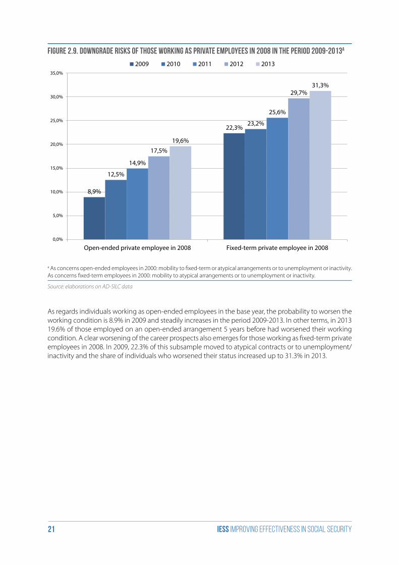
The AD-SILC dataset, tracking all workers up to the end of 2013 – apart from public employees that are tracked up to 2011 – allows us to observe individual prospects in the labour market during the current economic crisis. Therefore, following the same definition of statuses applied in the previous sections, we observe the transitions in the period 2009-2013 of those individuals employed as open-ended or fixed-term private employees in 2008 (excluding those who retired in the period of observation).
In detail, following the definitions used in section 2.3, we focus on downgrade risks computing two in-dicators (Figure 2.9): i) the share of open-ended private employees at the end of 2008 who in the subse-quent five years have moved towards fixed term or atypical arrangements or towards unemployment or inactivity; ii) the share of fixed-term private employees at the end of 2008 who in the subsequent five years have moved towards atypical arrangements or towards unemployment or inactivity.
iess Improving effectiveness in social security21
Figure 2.9. Downgrade risks of those working as private employees in 2008 in the period 2009-2013a
8,9%
22,3%
12,5%
23,2%
14,9%
25,6%
17,5%
29,7%
19,6%
31,3%
0,0%
5,0%
10,0%
15,0%
20,0%
25,0%
30,0%
35,0%
Open-ended private employee in 2008 Fixed-term private employee in 2008
2009 2010 2011 2012 2013
a As concerns open-ended employees in 2000: mobility to fixed-term or atypical arrangements or to unemployment or inactivity. As concerns fixed-term employees in 2000: mobility to atypical arrangements or to unemployment or inactivity.
Source: elaborations on AD-SILC data
As regards individuals working as open-ended employees in the base year, the probability to worsen the working condition is 8.9% in 2009 and steadily increases in the period 2009-2013. In other terms, in 2013 19.6% of those employed on an open-ended arrangement 5 years before had worsened their working condition. A clear worsening of the career prospects also emerges for those working as fixed-term private employees in 2008. In 2009, 22.3% of this subsample moved to atypical contracts or to unemployment/inactivity and the share of individuals who worsened their status increased up to 31.3% in 2013.

iess Improving effectiveness in social security22
Conclusions
Workers’ vulnerability cannot be assessed by looking at the individual employment status in a given point of time, but it is a condition that has to be empirically assessed studying the transition experienced by workers during their career among the several working statuses (e.g. temporary jobs, permanent em-ployment, unemployment, inactivity) in a dynamic perspective.
Hence, the main research idea behind this chapter has been to analyse by means of the longitudinal da-taset AD-SILC the interplay between contractual arrangements and individual prospects up to a twelve-year period.
Data signal that in the medium and long run individual working trajectories are various and often not linear, i.e. they differ from the mere “fixed-term at the entry, then permanent” dynamic, even before the explosion of the current recession phase. Temporary workers are relatively more at risk and are often trapped in disadvantaged statuses (especially when working through atypical arrangements), but, more in general, the majority of workers, independently from their contractual status, record a non-negligible probability of changing status.
Transitions regarding the stock of workers signal that the Italian labour market has never truly been very rigid. In particular, medium and long-term persistence in open-ended employment are always very far from 100% and frequent movements outside the active labour force are observed. The frequency of people losing the status of permanent employee at least once in a five-year period is high (41%), even if risks are higher for weaker workers (e.g. low skilled, females, living in the South and working in small size firms). Furthermore, the crisis greatly exacerbated workers’ vulnerability, as can be assessed by looking at the share of employees who worsened their contractual arrangement in the period 2009-2013.
The empirical evidence observed in this chapter suggests that the Italian labour market seems characte-rized by a sort of “liquidity” rather than by a simple segmentation between insiders and outsiders, becau-se a very large share of individuals continuously rise and fall among relatively advantaged and disadvan-taged statuses.
iess Improving effectiveness in social security23
3. The new versions of T-DYMM
Introduction
In this chapter, we focus on the new version of the Treasury Dynamic Microsimulation Model (henceforth, TDYMM 2.0), describing its characteristics and functions. The new model T-DYMM 2.0 contains a few dif-ferences compared to the previous release, in particular:
i) A new simulation platform LIAM2, that represents a natural evolution of the previously employed LIAM;
ii) Some changes on the structure of the main modules that compose the model (demographic, labour market and pension module);
iii) The extension of the model with an extra sub-module that allows to analyse the dynamics of pri-vate pension schemes.
The chapter contains three paragraphs. Section 3.1 summarises the recent history of T-DYMM 1.0: the birth and the structure of the first DMSM. Section 3.2 gives an overview of the new T-DYMM 2.0 compo-nents, highlighting the most important progress of the model on the demographic and pension modu-les. The last section presents the external tax module.
3.1 Recent history of T-DYMM: the first release of the model
The first release of T-DYMM (henceforth, T-DYMM 1.0) is a dynamic microsimulation model (DMSM), which significantly benefits and moves from the experience of MIDAS-IT6, a DMSM written by the ISAE (the Italian Institute for Studies and Economic Analyses)7.
T-DYMM 1.0 has the Italian population as a base. It simulates the evolution of a cross-sectional sample representative of the population, with both individuals and households as units of analysis.
Following O’Donoghue’s (2001) taxonomy, T-DYMM 1.0 presents the following features:
i) It is a model with dynamic ageing;
ii) It is a discrete time model: transitions in the labour market and all updating processes are carried out year-by-year;
iii) The ageing process is probabilistic: simulation and transitional dynamics are achieved through probabilistic methodologies. In particular, discrete transitions (in the labour market or in others sec-tions) are obtained by means of a Monte Carlo technique;
6 http://www.bancaditalia.it/studiricerche/convegni/atti/pensionreform/Session3/Dekkers_et_al.pdf. 7 The model was developed in the context of AIM, a European‐funded sixth framework project. http://aei.pitt.edu/10747/1/1780.pdf.
iess Improving effectiveness in social security24
iv) It is a closed model: it simulates life-cycle evolution of the main demographic and economic po-pulation features within the sample, with new individuals that enter the population each year due to birth and others who exit due to death. As of now, migration flows are not simulated.
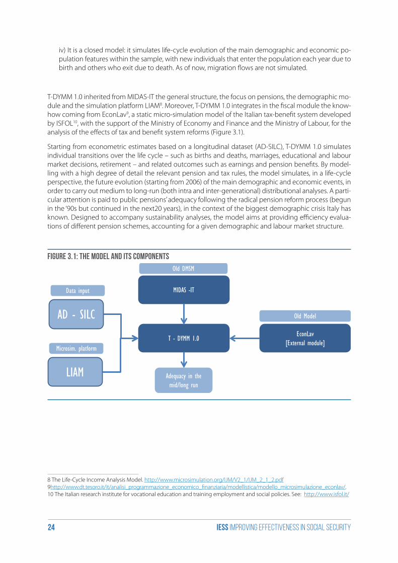
T-DYMM 1.0 inherited from MIDAS-IT the general structure, the focus on pensions, the demographic mo-dule and the simulation platform LIAM8. Moreover, T-DYMM 1.0 integrates in the fiscal module the know-how coming from EconLav9, a static micro-simulation model of the Italian tax-benefit system developed by ISFOL10, with the support of the Ministry of Economy and Finance and the Ministry of Labour, for the analysis of the effects of tax and benefit system reforms (Figure 3.1).
Starting from econometric estimates based on a longitudinal dataset (AD-SILC), T-DYMM 1.0 simulates individual transitions over the life cycle – such as births and deaths, marriages, educational and labour market decisions, retirement – and related outcomes such as earnings and pension benefits. By model-ling with a high degree of detail the relevant pension and tax rules, the model simulates, in a life-cycle perspective, the future evolution (starting from 2006) of the main demographic and economic events, in order to carry out medium to long-run (both intra and inter-generational) distributional analyses. A parti-cular attention is paid to public pensions’ adequacy following the radical pension reform process (begun in the ‘90s but continued in the next20 years), in the context of the biggest demographic crisis Italy has known. Designed to accompany sustainability analyses, the model aims at providing efficiency evalua-tions of different pension schemes, accounting for a given demographic and labour market structure.
Figure 3.1: The Model and its components
MIDAS -IT
T - DYMM 1.0
AD - SILCEconLav
[External module]
Adequacy in the mid/long run
Data input
Old DMSM
Old Model
LIAM
Microsim. platform
8 The Life-Cycle Income Analysis Model. http://www.microsimulation.org/IJM/V2_1/IJM_2_1_2.pdf 9 http://www.dt.tesoro.it/it/analisi_programmazione_economico_finanziaria/modellistica/modello_microsimulazione_econlav/.10 The Italian research institute for vocational education and training employment and social policies. See: http://www.isfol.it/
iess Improving effectiveness in social security25
The stylised structure of the model consists of three main modules linked to each other by recursive feedbacks (i.e. in the same period the causal relationship is unidirectional), then integrated with a fourth (so far external) one regarding the taxation system. In detail, T-DYMM 1.0 comprises:
1. A Demographic module, inherited by MIDAS (Dekkers et al., 2009); it estimates intergenerational persistence, birth processes, educational achievements and the “marriage market”.
2. A Labour market module that probabilistically simulates individual labour market dynamics, na-mely employment transitions (in and out of the labour market and among employment categories, sectors and contractual arrangements).
3. A Pension module for the definition of eligibility requirements and retirement decisions and for the computation of pension benefits.
4. A Fiscal module, running separately at the end of the simulation process, that produces net labour and pension incomes, with a high degree of detail on the Italian tax-benefit system.
T-DYMM 1.0 uses alignment procedures (i.e. calibrations) – in particular in the demographic module – in order to link certain aggregate results (couples formation, fertility and mortality rates, employment rates, disability rates) to official projections. The main source of alignment is the Ageing Working Group, (AWG)11 2015, Ageing Report baseline demographic and macroeconomic projections for the period 2006-2060.
3.2 The new release of the model: from T-DYMM 1.0 to T-DYMM 2.0
T-DYMM 2.0 – like its predecessor – is based on econometric estimates carried out on a new longitudinal dataset and its key aim is to simulate individuals’ transitions over life cycle (births, deaths, marriages, edu-cational and labour market decisions, retirement) and analyse their condition at retirement.
In the present section, we present the most important characteristics of T-DYMM 2.0, highlighting the main differences between the new and the old version of the model and focusing on four main points:
i) the new platform of the simulation with a new programming code (LIAM2);
ii) the new structure of the model and the new characteristics of the modules;
iii) T-DYMM 2.0‘s complete departure from MIDAS – IT estimates;
iv) the new sub-module on private pension schemes (henceforth, PPS).
3.2.1 The new simulation platform
The model operates on the new simulation platform LIAM2, that represents a natural evolution of the previously employed LIAM and provides considerable improvements in terms of speed and data capa-city.
LIAM2 is a generic microsimulation modelling toolbox, which allows to develop almost any microsimu-lation model as long as it uses cross-sectional ageing. Being it an open-source tool12, and with the incre-ased cooperation through meetings and code sharing, LIAM2 should greatly reduce the development
11 http://ec.europa.eu/economy_finance/publications/european_economy/2012/pdf/ee-2012-2_en.pdf.12 It is licensed under the GNU General Public License (GPL) version 3.
iess Improving effectiveness in social security26
costs (in terms of both time and money) of microsimulation models. It should enable the use of very large datasets, such as AD-SILC, or even the expansion of the survey data to the whole population in order to fulfil representativeness requirements. Due to its new programming code, LIAM213 – in the version 0.11 – is much more flexible and increases the simulation scopes. The platform’s interface is very friendly and allows for an easy and flexible use for microsimulation team.
Most of all, LIAM2 is much faster than its predecessor, reducing time costs for each simulation by about ten times.
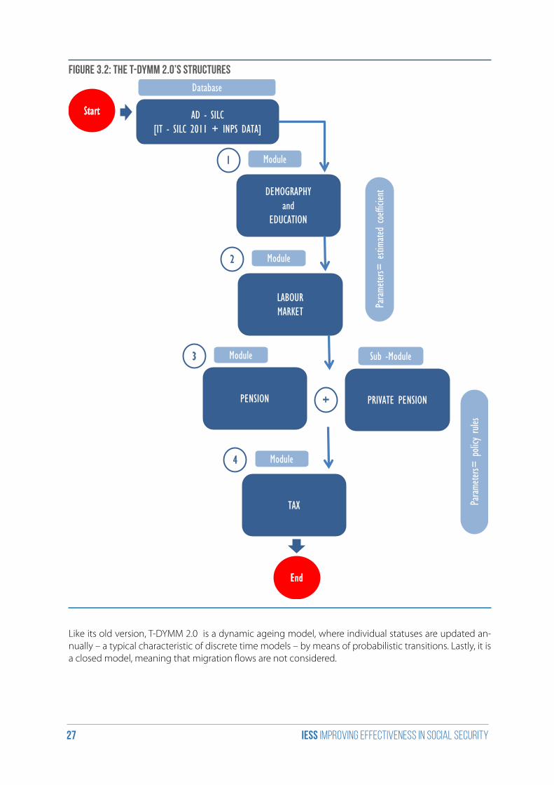
3.2.2 The new structure of the model and the new characteristics of the modules
T-DYMM 2.0 (Figure 3.2) has maintained the general structure and features of the previous version (T-DYMM 1.0). It consists of three main modules linked to each other by recursive feedback, plus a fourth external module (Tax module) as in the case of the previous version of the DMSM. In particular, T-DYMM 2.0 is composed of:
• a Demographic module;
• a Labour market module;
• a Pension module (with a sub-module on private pension schemes);
• a Tax module (external).
13 http://liam2.plan.be/
iess Improving effectiveness in social security27
Figure 3.2: The T-DYMM 2.0’s structures
Start AD - SILC[IT - SILC 2011 + INPS DATA]
Database
1 Module
DEMOGRAPHYand
EDUCATION
2 Module
LABOURMARKET
PENSION
4 Module
TAX
Param
eters=
estim
ated
coeff
icient
+ PRIVATE PENSION
3 Module Sub -Module
Param
eters=
policy rules
End
Like its old version, T-DYMM 2.0 is a dynamic ageing model, where individual statuses are updated an-nually – a typical characteristic of discrete time models – by means of probabilistic transitions. Lastly, it is a closed model, meaning that migration flows are not considered.

iess Improving effectiveness in social security28
In the model, all the monetary values (gross income, pensions and other welfare benefits) are expressed in real terms. Generally, welfare rules establish that monetary parameters and cash benefits – e.g. “As-segno sociale”, “Integrazione al minimo”, etc. – are indexed to inflation. T-DYMM 2.0 does not account for inflation variations, and assumes that these monetary values are instead indexed to GDP real growth, as projected by AWG14.
The main purpose of T-DYMM 2.0 is to analyse the adequacy of the Italian pension system in the medium-long run. Yet, it is worth highlighting that the model is very flexible and can support other secondary objectives, e.g., simulating pension reforms or analysing the impact of labour market reforms and even-tually assessing the sustainability of the pension system.
3.2.3 Demographic module
T-DYMM 2.0’s demographic module estimates intergenerational persistence, birth processes, educatio-nal achievements and the “marriage market”. Differently from T-DYMM 1.0’s module, estimates are no lon-ger taken from MIDAS-IT. Indeed, in T-DYMM 2.0 all econometric regressions have been based exclusively on the new version of AD-SILC15, ensuring more reliable and suitable estimations. The module simulates four types of processes (Table 3.1):
Table 3.1: Demographic module
Process Description Alignment
1 Alive Individuals are assigned to either life or death AWG 2015
2 Birth Which and how many women give birth AWG 2015
3 EducationThree levels: Compulsory, upper-secondary and universi-ty level. Achievement dependent on parental education
Istat
4 Marriage marketCoupling process (marriage or cohabitation). Divorce/se-paration process
Internal
These processes can be aggregated in three kinds of demographic events (or choices):
1. events that mainly modify the population structure by sub-group composition, such as mortality and fertility rates. So far, survival probabilities are not tested by any micro-level analysis, and mortality is uniformly distributed among ages and genders according to AWG 2015 projections16. On the other hand, the birth process includes the consideration of certain parameters pertaining to women in fertile age, so that the most likely to give birth are selected. Fertility rates are taken from AWG 2015 projections;
2. attribution of an educational level (compulsory, upper-secondary or university level) to young pe-ople (in education age), which is simulated on the basis of parental education. The shares of indivi-duals assigned to the each education achievement are aligned to Istat official statistics and projected in the future with a logarithmic function17;
14 This procedure allows accounting for a necessary periodical update of said parameters by the policy maker. A mere index-ation to inflation, in a context of economic growth, would greatly penalize the mentioned social benefits in the long run.15 See chapter 4.16 http://ec.europa.eu/economy_finance/publications/european_economy/2014/pdf/ee8_en.pdf.17 See chapter 4, paragraph 4.1.
iess Improving effectiveness in social security29
3. events that affect the household structure, such as departure from the family of origin, cohabita-tion, marriage and separation. The matching process among singles and the divorce process among in-couple individuals are estimated via AD-SILC variables. Based on the baseline data, specific ali-gnments are developed in order to keep the number of coupled individuals and of divorcees con-stant overtime. This “neutrality assumption” seems appropriate in a context where such demographic phenomena do not constitute the “reason why” of the research.
3.2.4 Labour market module
The labour market module has two main purposes: on one hand, it simulates the transitions between different employment states; on the other, once a labour market status is established, the corresponding level of income is imputed.
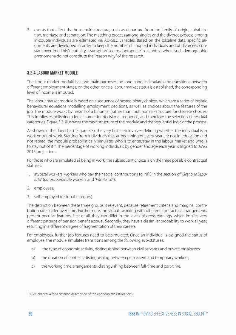
The labour market module is based on a sequence of nested binary choices, which are a series of logistic behavioural equations modelling employment decisions, as well as choices about the features of the job. The module works by means of a binomial (rather than multinomial) structure for discrete choices. This implies establishing a logical order for decisional sequence, and therefore the selection of residual categories. Figure 3.3 illustrates the basic structure of the module and the sequential logic of the process.
As shown in the flow chart (Figure 3.3), the very first step involves defining whether the individual is in work or out of work. Starting from individuals that at beginning of every year are not in education and not retired, the module probabilistically simulates who is to enter/stay in the labour market and who is to stay out of it18. The percentage of working individuals by gender and age each year is aligned to AWG 2015 projections.
For those who are simulated as being in work, the subsequent choice is on the three possible contractual statuses:
1. atypical workers: workers who pay their social contributions to INPS in the section of “Gestione Sepa-rata” (parasubordinate workers and “Partite Iva”);
2. employees;
3. self-employed (residual category).
The distinction between these three groups is relevant, because retirement criteria and marginal contri-bution rates differ over time. Furthermore, individuals working with different contractual arrangements present peculiar features. First of all, they can differ in the levels of gross earnings, which implies very different patterns of pension benefit accrual. Secondly, they have a dissimilar probability to work all year, resulting in a different degree of fragmentation of their careers.
For employees, further job features need to be simulated. Once an individual is assigned the status of employee, the module simulates transitions among the following sub-statuses:
a) the type of economic activity, distinguishing between civil servants and private employees;
b) the duration of contract, distinguishing between permanent and temporary workers;
c) the working time arrangements, distinguishing between full-time and part-time.
18 See chapter 4 for a detailed description of the econometric estimations.
iess Improving effectiveness in social security30
Figure 3.3: Labour market module
NOTIN WORK
NOT IN EDUCATION and NOT RETIRED
IN WORK
ATYPICAL WORKERS[Gestione Sep. INPS= P. iva+Parasubordinate workers]
EMPLOYEES
SELF EMPLOYED WORKERS[Residual category]
CIVIL SERVANTS
PERMANENT WORKERS
PART TIME/FULL TIME
DISABLED
OTHER INACTIVE
Months worked
In work all year
Gross earnings or salary
+
+
Once an individual is assigned to a particular employment status, the following step is the simulation of a yearly labour gross income. This is the measure of earnings that represents the base on which contribu-tion rates have to be applied in order to calculate the contribution to future pension benefits19.
Finally, it is important to underline that a part of the individuals out of work every year are assigned to the “disabled” category. For simplicity’s sake, we assume that these workers are permanently out of the work force. Information on disability is extracted from AD-SILC, and in accordance with T-DYMM 1.0 ad hoc alignments are built in order to keep the number of disabled individuals constant over the simulation period.
3.2.5 Pension module
The pension module in T-DYMM 2.0 is divided in two parts:
1. simulation of pensions of the first pillar (public pensions);
2. simulation of pensions of the second and third pillars (private pensions).
19 See chapter 4 for a detailed description of the gross income econometric estimations.
iess Improving effectiveness in social security31
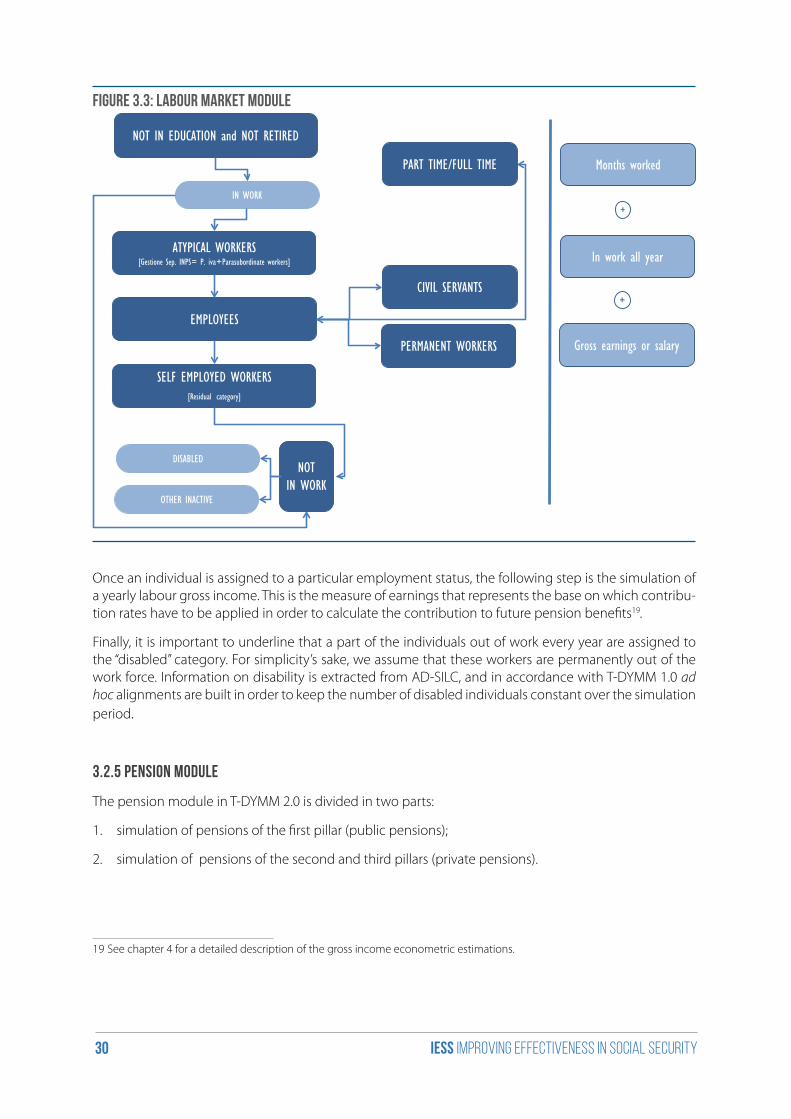
3.2.5.1 Public pension sub-module
The public pension module (henceforth, PubPM) comprises three steps that define the sequence of the process (Figure 3.4):
a) deposit of contribution;
b) pension benefit calculation;
c) verification of eligibility requirements and attribution of retirement decisions.
Figure 3.4: Public Pension module
DEPOSIT OF CONTRIBUTIONS
RETIREMENT DECISION
BENEFIT INDEXATION
NOTIN WORK
ELIGIBILITY REQUIREMENTS
PENSION BENFIT CALCULATION
The PubPM starts with the simulation of seniority and social contributions accrual. For each individual in work, seniority increases according to the time spent in employment during the year. For what concerns contri-butions accrual, the model applies the appropriate contribution rates (they vary over time and for different employment categories) to gross labour incomes in order to compute the pension notional annual savings.
Once these steps are completed, the module computes the potential pension benefits according to the rules for each pension regime, described in Table 3.2. The module classifies each worker in the appropria-te pension scheme: “Mixed 1995”20, “Mixed 2011”21 or “NDC”22. In-sample individuals are assigned to their pension scheme according to their seniority level in 1995, new-borns are automatically assigned to the Notional Defined Contribution regime.
20 Workers who had at least 18 years of seniority in 1995. Defined Benefit rules are applied pro-quota for the share of seniority accrued prior to Jan 1st 2012. Notional Defined Contribution rules are applied for the remaining quota.21 Workers who had less than 18 years of seniority in 1995. Defined Benefit rules are applied pro-quota for the share of senior-ity accrued prior to Jan 1st 1996 on overall seniority. Notional Defined Contribution rules are applied for the remaining quota.22 Individuals who have started working after 1995 who are subject to a full Notional Defined Contribution (NDC) scheme.
iess Improving effectiveness in social security32
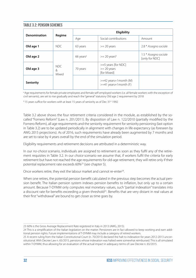
Table 3.2: Pension schemes
Denomination RegimeEligibility
Age Social contributions Amount
Old age 1 NDC 63 years >= 20 years 2.8 * Assegno sociale
Old age 2
NDC&Mixed
66 yearsa >= 20 yearsb 1.5 * Assegno sociale[only for NDC]
Old age 3 70 years>=5 years [for NDC]>= 20 years[for Mixed]
Seniority >=42 years+1month (M)>=41 years+1month (F)
a Age requirements for female private employees and female self-employed workers (i.e. all female workers with the exception of civil servants), are set to rise gradually and reach the “general” statutory Old age 2 requirement by 2018
b 15 years suffice for workers with at least 15 years of seniority as of Dec 31st 1992
Table 3.2 above shows the four retirement criteria considered in the module, as established by the so-called “Fornero Reform” (Law n. 201/2011). By disposition of Law n. 122/2010 (partially modified by the Fornero Reform), all age requirements and the seniority requirement for seniority pensioning (last option in Table 3.2) are to be updated periodically in alignment with changes in life expectancy (as foreseen by AWG 2015 projections). As of 2016, such requirements have already been augmented by 7 months and are set to raise by 4 years overall by the end of the simulation period.
Eligibility requirements and retirement decisions are attributed in a deterministic way.
In our no-choice scenario, individuals are assigned to retirement as soon as they fulfil any of the retire-ment requisites in Table 3.2. In our choice scenario we assume that, if workers fulfil the criteria for early retirement but have not reached the age requirements for old-age retirement, they will retire only if their potential replacement rate exceeds 60%23 (see chapter 5).
Once workers retire, they exit the labour market and cannot re-enter24.
When one retires, the potential pension benefit calculated in the previous step becomes the actual pen-sion benefit. The Italian pension system indexes pension benefits to inflation, but only up to a certain amount. Because T-DYMM only computes real monetary values, such “partial indexation” translates into a discount rate for benefits exceeding a given threshold25. Benefits that are very distant in real values at their first “withdrawal” are bound to get closer as time goes by.
23 60% is the Gross Average Replacement Rate registered in Italy in 2013 (AWG, 2015).24 This is a simplification of the Italian legislation on the matter. Pensioners are in fact allowed to keep working and earn addi-tional pension rights. Future implementations of T-DYMM may include a category of retired workers.25 A recent ruling from the Italian Constitutional Court (n. 70/2015) declared the halt to indexation for years 2012-2013 uncon-stitutional. With Decree Law n. 65/2015, pensions whose indexation was halted were somewhat reimbursed. This is all simulated within T-DYMM, thus allowing for an evaluation of the actual impact in adequacy terms of Law Decree n. 65/2015.
iess Improving effectiveness in social security33
In addition to ordinary old-age and early retirement pension benefits, the pension module simulates other kinds of benefits:
i) survivor’s pensions, paid to the retiree’s widow/er;
ii) social pensions (“assegno sociale”), e.g. non-contributory means-tested social allowances paid to the elderly26;
iii) minimum integrations (“integrazione al minimo”), e.g. non-contributory benefits – only available to individuals enrolled, entirely or pro quota, in the old Defined Benefit scheme – paid out whenever benefits are below the minimum level;
iv) disability pensions paid to workers whose earning capacity is reduced due to illness27.
The procedure for the attribution of survivor’s pensions and non-contributory pensions mirrors the Ita-lian law requirements; eligibility for such benefits depends on both individual’s and household’s incomes of applicants.
3.2.5.2 Private pension sub-module
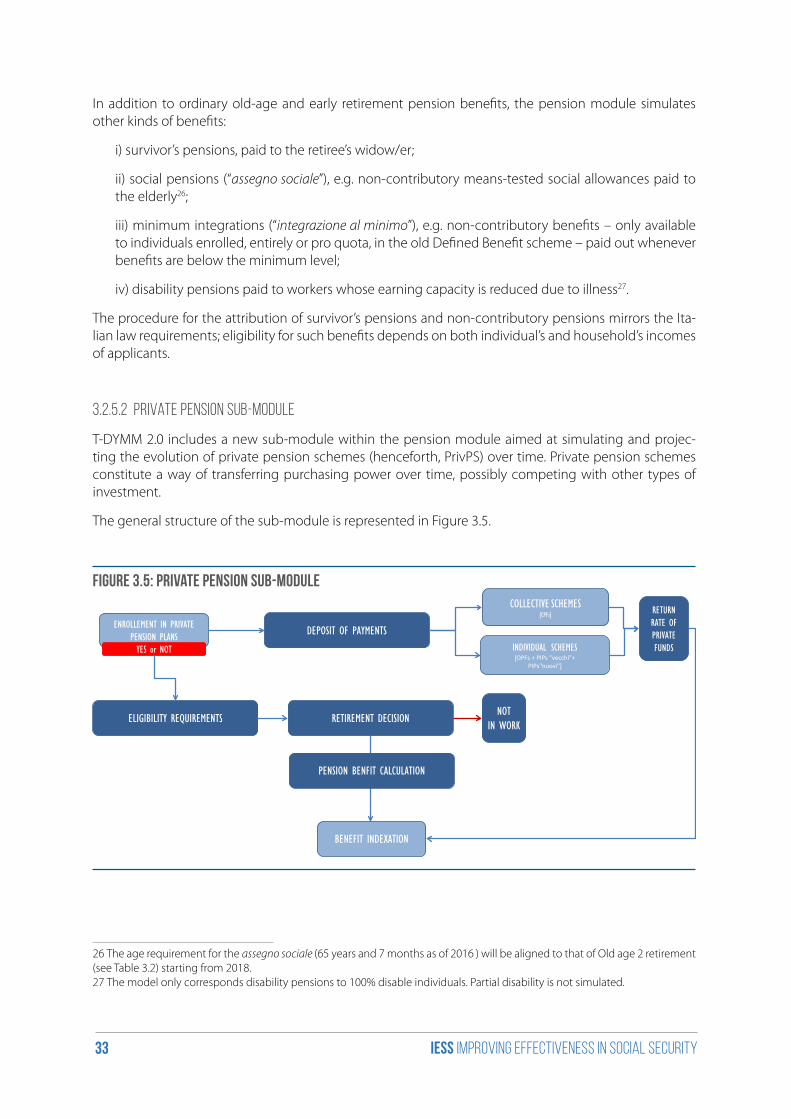
T-DYMM 2.0 includes a new sub-module within the pension module aimed at simulating and projec-ting the evolution of private pension schemes (henceforth, PrivPS) over time. Private pension schemes constitute a way of transferring purchasing power over time, possibly competing with other types of investment.
The general structure of the sub-module is represented in Figure 3.5.
Figure 3.5: Private pension sub-module
DEPOSIT OF PAYMENTS
RETIREMENT DECISIONNOT
IN WORKELIGIBILITY REQUIREMENTS
PENSION BENFIT CALCULATION
ENROLLEMENT IN PRIVATE PENSION PLANSYES or NOT INDIVIDUAL SCHEMES
[OPFs + PIPs "vecchi"+PIPs"nuovi"]
COLLECTIVE SCHEMES[CPFs] RETURN
RATE OF PRIVATE FUNDS
BENEFIT INDEXATION
26 The age requirement for the assegno sociale (65 years and 7 months as of 2016 ) will be aligned to that of Old age 2 retirement (see Table 3.2) starting from 2018.27 The model only corresponds disability pensions to 100% disable individuals. Partial disability is not simulated.
iess Improving effectiveness in social security34
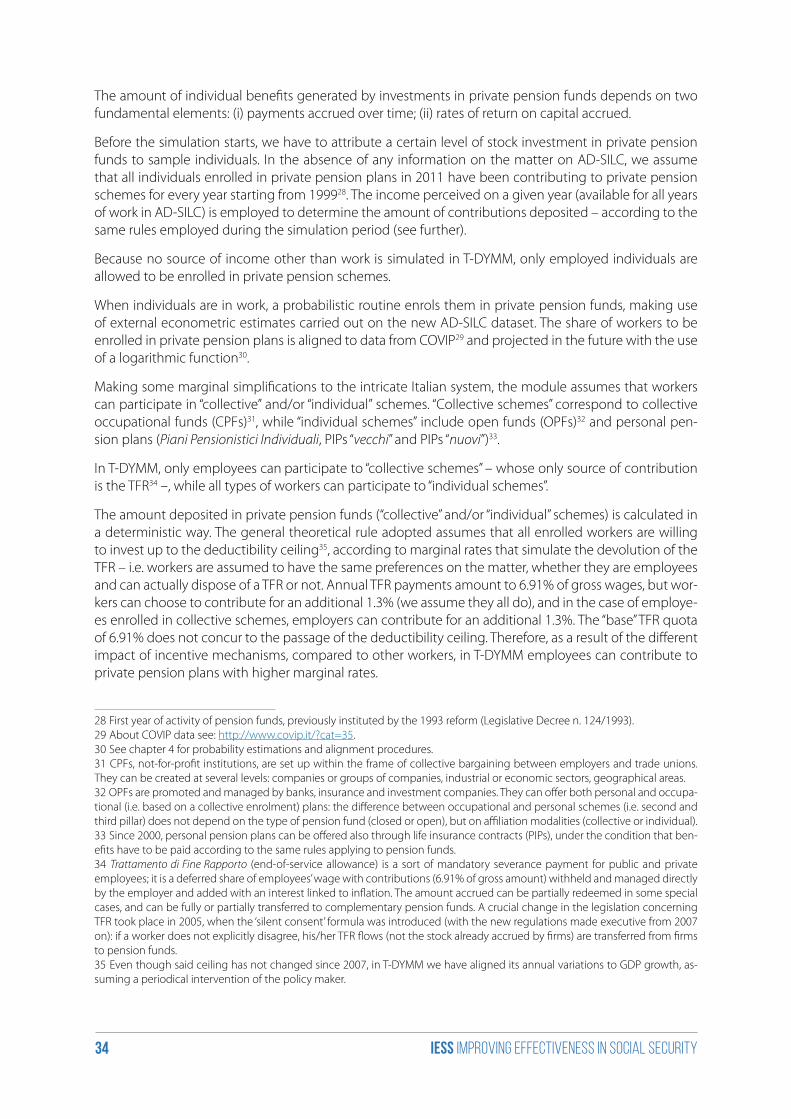
The amount of individual benefits generated by investments in private pension funds depends on two fundamental elements: (i) payments accrued over time; (ii) rates of return on capital accrued.
Before the simulation starts, we have to attribute a certain level of stock investment in private pension funds to sample individuals. In the absence of any information on the matter on AD-SILC, we assume that all individuals enrolled in private pension plans in 2011 have been contributing to private pension schemes for every year starting from 199928. The income perceived on a given year (available for all years of work in AD-SILC) is employed to determine the amount of contributions deposited – according to the same rules employed during the simulation period (see further).
Because no source of income other than work is simulated in T-DYMM, only employed individuals are allowed to be enrolled in private pension schemes.
When individuals are in work, a probabilistic routine enrols them in private pension funds, making use of external econometric estimates carried out on the new AD-SILC dataset. The share of workers to be enrolled in private pension plans is aligned to data from COVIP29 and projected in the future with the use of a logarithmic function30.
Making some marginal simplifications to the intricate Italian system, the module assumes that workers can participate in “collective” and/or “individual” schemes. “Collective schemes” correspond to collective occupational funds (CPFs)31, while “individual schemes” include open funds (OPFs)32 and personal pen-sion plans (Piani Pensionistici Individuali, PIPs “vecchi” and PIPs “nuovi”)33.
In T-DYMM, only employees can participate to “collective schemes” – whose only source of contribution is the TFR34 –, while all types of workers can participate to “individual schemes”.
The amount deposited in private pension funds (“collective” and/or “individual” schemes) is calculated in a deterministic way. The general theoretical rule adopted assumes that all enrolled workers are willing to invest up to the deductibility ceiling35, according to marginal rates that simulate the devolution of the TFR – i.e. workers are assumed to have the same preferences on the matter, whether they are employees and can actually dispose of a TFR or not. Annual TFR payments amount to 6.91% of gross wages, but wor-kers can choose to contribute for an additional 1.3% (we assume they all do), and in the case of employe-es enrolled in collective schemes, employers can contribute for an additional 1.3%. The “base” TFR quota of 6.91% does not concur to the passage of the deductibility ceiling. Therefore, as a result of the different impact of incentive mechanisms, compared to other workers, in T-DYMM employees can contribute to private pension plans with higher marginal rates.
28 First year of activity of pension funds, previously instituted by the 1993 reform (Legislative Decree n. 124/1993).29 About COVIP data see: http://www.covip.it/?cat=35. 30 See chapter 4 for probability estimations and alignment procedures.31 CPFs, not-for-profit institutions, are set up within the frame of collective bargaining between employers and trade unions. They can be created at several levels: companies or groups of companies, industrial or economic sectors, geographical areas.32 OPFs are promoted and managed by banks, insurance and investment companies. They can offer both personal and occupa-tional (i.e. based on a collective enrolment) plans: the difference between occupational and personal schemes (i.e. second and third pillar) does not depend on the type of pension fund (closed or open), but on affiliation modalities (collective or individual).33 Since 2000, personal pension plans can be offered also through life insurance contracts (PIPs), under the condition that ben-efits have to be paid according to the same rules applying to pension funds.34 Trattamento di Fine Rapporto (end-of-service allowance) is a sort of mandatory severance payment for public and private employees; it is a deferred share of employees’ wage with contributions (6.91% of gross amount) withheld and managed directly by the employer and added with an interest linked to inflation. The amount accrued can be partially redeemed in some special cases, and can be fully or partially transferred to complementary pension funds. A crucial change in the legislation concerning TFR took place in 2005, when the ‘silent consent’ formula was introduced (with the new regulations made executive from 2007 on): if a worker does not explicitly disagree, his/her TFR flows (not the stock already accrued by firms) are transferred from firms to pension funds.35 Even though said ceiling has not changed since 2007, in T-DYMM we have aligned its annual variations to GDP growth, as-suming a periodical intervention of the policy maker.
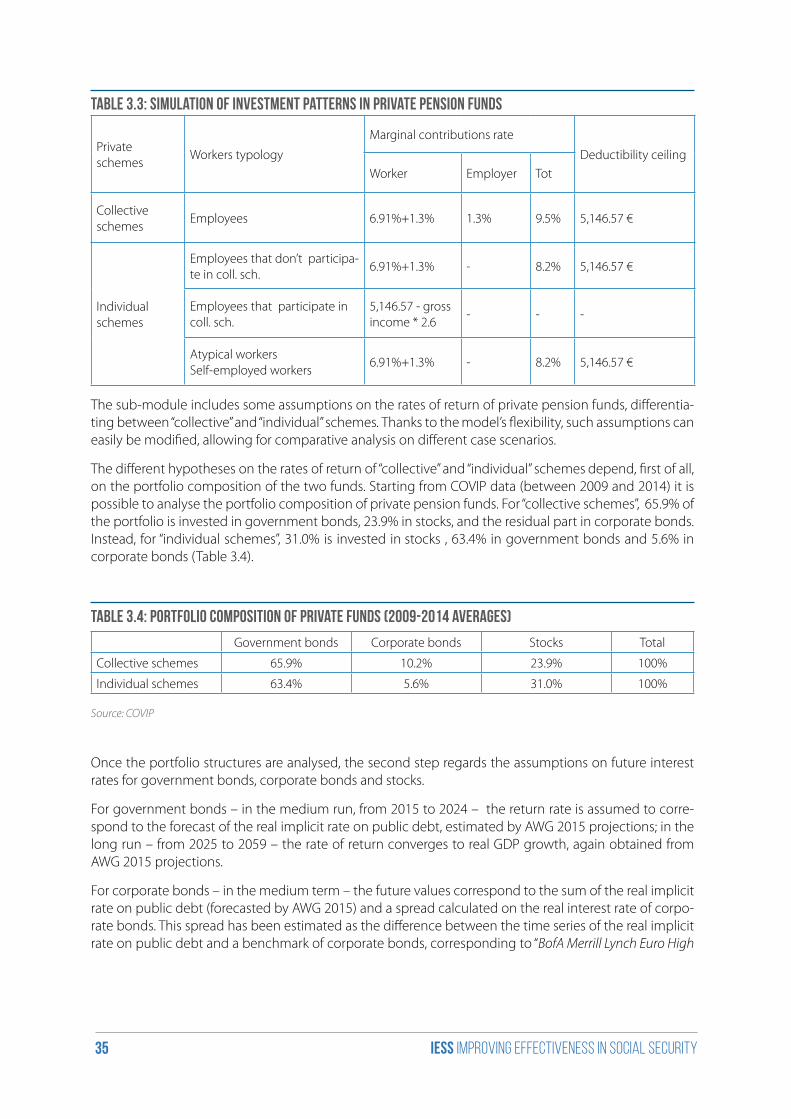
iess Improving effectiveness in social security35
Table 3.3: Simulation of investment patterns in private pension funds
Private schemes
Workers typology
Marginal contributions rate
Deductibility ceilingWorker Employer Tot
Collective schemes
Employees 6.91%+1.3% 1.3% 9.5% 5,146.57 €
Individual schemes
Employees that don’t participa-te in coll. sch.
6.91%+1.3% - 8.2% 5,146.57 €
Employees that participate in coll. sch.
5,146.57 - gross income * 2.6
- - -
Atypical workersSelf-employed workers
6.91%+1.3% - 8.2% 5,146.57 €
The sub-module includes some assumptions on the rates of return of private pension funds, differentia-ting between “collective” and “individual” schemes. Thanks to the model’s flexibility, such assumptions can easily be modified, allowing for comparative analysis on different case scenarios.
The different hypotheses on the rates of return of “collective” and “individual” schemes depend, first of all, on the portfolio composition of the two funds. Starting from COVIP data (between 2009 and 2014) it is possible to analyse the portfolio composition of private pension funds. For “collective schemes”, 65.9% of the portfolio is invested in government bonds, 23.9% in stocks, and the residual part in corporate bonds. Instead, for “individual schemes”, 31.0% is invested in stocks , 63.4% in government bonds and 5.6% in corporate bonds (Table 3.4).
Table 3.4: Portfolio composition of private funds (2009-2014 averages)
Government bonds Corporate bonds Stocks Total
Collective schemes 65.9% 10.2% 23.9% 100%
Individual schemes 63.4% 5.6% 31.0% 100%
Source: COVIP
Once the portfolio structures are analysed, the second step regards the assumptions on future interest rates for government bonds, corporate bonds and stocks.
For government bonds – in the medium run, from 2015 to 2024 – the return rate is assumed to corre-spond to the forecast of the real implicit rate on public debt, estimated by AWG 2015 projections; in the long run – from 2025 to 2059 – the rate of return converges to real GDP growth, again obtained from AWG 2015 projections.
For corporate bonds – in the medium term – the future values correspond to the sum of the real implicit rate on public debt (forecasted by AWG 2015) and a spread calculated on the real interest rate of corpo-rate bonds. This spread has been estimated as the difference between the time series of the real implicit rate on public debt and a benchmark of corporate bonds, corresponding to “BofA Merrill Lynch Euro High
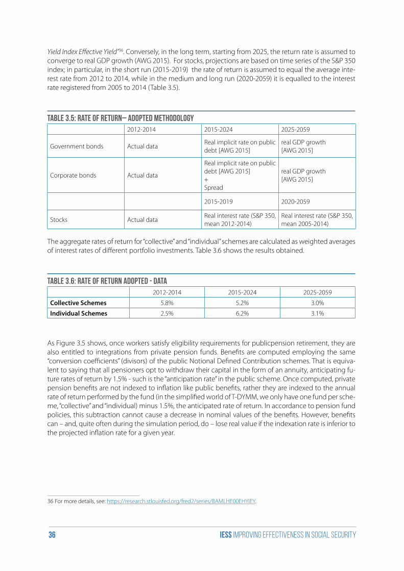
iess Improving effectiveness in social security36
Yield Index Effective Yield”36. Conversely, in the long term, starting from 2025, the return rate is assumed to converge to real GDP growth (AWG 2015). For stocks, projections are based on time series of the S&P 350 index; in particular, in the short run (2015-2019) the rate of return is assumed to equal the average inte-rest rate from 2012 to 2014, while in the medium and long run (2020-2059) it is equalled to the interest rate registered from 2005 to 2014 (Table 3.5).
Table 3.5: Rate of return– adopted methodology2012-2014 2015-2024 2025-2059
Government bonds Actual dataReal implicit rate on public debt [AWG 2015]
real GDP growth[AWG 2015]
Corporate bonds Actual data
Real implicit rate on public debt [AWG 2015]+Spread
real GDP growth[AWG 2015]
2015-2019 2020-2059
Stocks Actual dataReal interest rate (S&P 350, mean 2012-2014)
Real interest rate (S&P 350, mean 2005-2014)
The aggregate rates of return for “collective” and “individual” schemes are calculated as weighted averages of interest rates of different portfolio investments. Table 3.6 shows the results obtained.
Table 3.6: Rate of return adopted - data2012-2014 2015-2024 2025-2059
Collective Schemes 5.8% 5.2% 3.0%
Individual Schemes 2.5% 6.2% 3.1%
As Figure 3.5 shows, once workers satisfy eligibility requirements for publicpension retirement, they are also entitled to integrations from private pension funds. Benefits are computed employing the same “conversion coefficients” (divisors) of the public Notional Defined Contribution schemes. That is equiva-lent to saying that all pensioners opt to withdraw their capital in the form of an annuity, anticipating fu-ture rates of return by 1.5% - such is the “anticipation rate” in the public scheme. Once computed, private pension benefits are not indexed to inflation like public benefits, rather they are indexed to the annual rate of return performed by the fund (in the simplified world of T-DYMM, we only have one fund per sche-me, “collective” and “individual) minus 1.5%, the anticipated rate of return. In accordance to pension fund policies, this subtraction cannot cause a decrease in nominal values of the benefits. However, benefits can – and, quite often during the simulation period, do – lose real value if the indexation rate is inferior to the projected inflation rate for a given year.
36 For more details, see: https://research.stlouisfed.org/fred2/series/BAMLHE00EHYIEY.
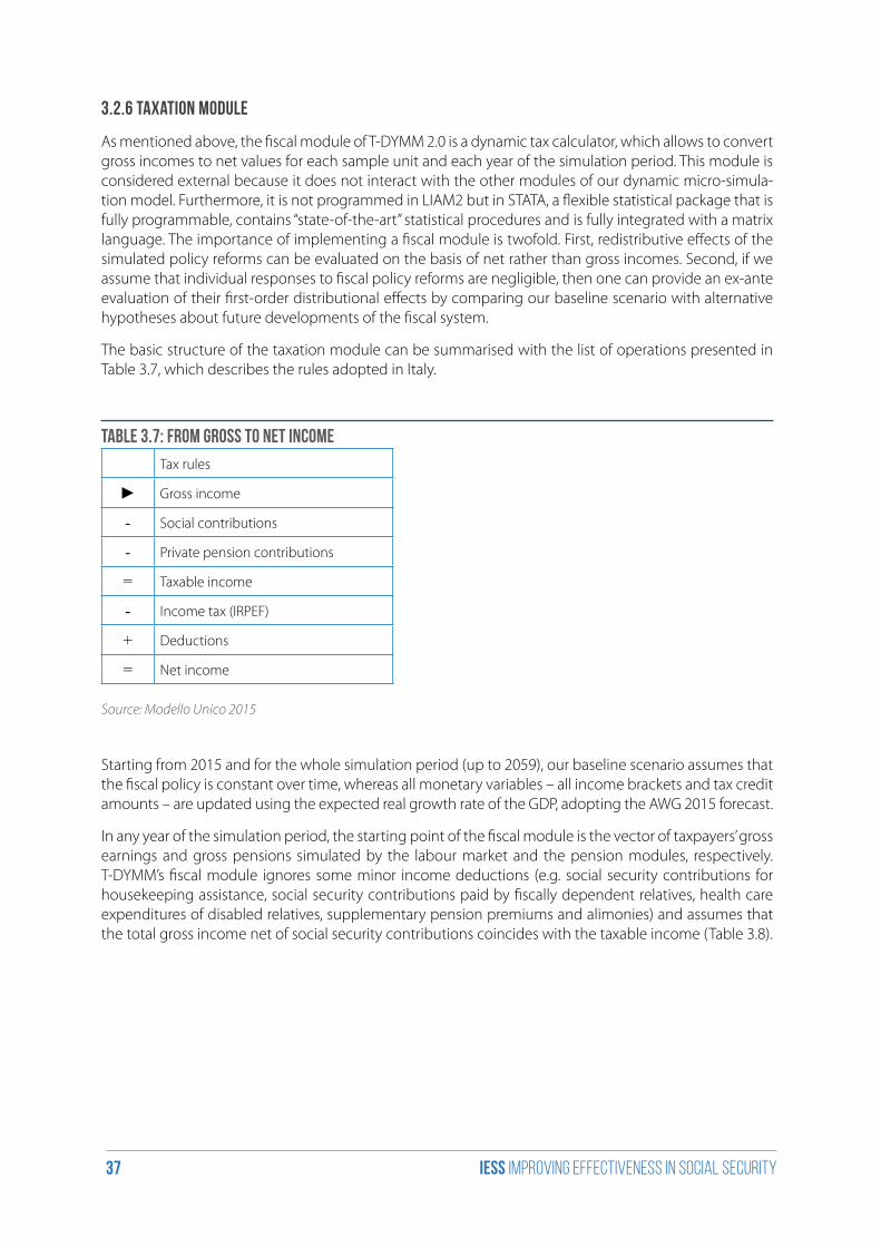
iess Improving effectiveness in social security37
3.2.6 Taxation module
As mentioned above, the fiscal module of T-DYMM 2.0 is a dynamic tax calculator, which allows to convert gross incomes to net values for each sample unit and each year of the simulation period. This module is considered external because it does not interact with the other modules of our dynamic micro-simula-tion model. Furthermore, it is not programmed in LIAM2 but in STATA, a flexible statistical package that is fully programmable, contains “state-of-the-art” statistical procedures and is fully integrated with a matrix language. The importance of implementing a fiscal module is twofold. First, redistributive effects of the simulated policy reforms can be evaluated on the basis of net rather than gross incomes. Second, if we assume that individual responses to fiscal policy reforms are negligible, then one can provide an ex-ante evaluation of their first-order distributional effects by comparing our baseline scenario with alternative hypotheses about future developments of the fiscal system.
The basic structure of the taxation module can be summarised with the list of operations presented in Table 3.7, which describes the rules adopted in Italy.
Table 3.7: From gross to net income
Tax rules
► Gross income
- Social contributions
- Private pension contributions
= Taxable income
- Income tax (IRPEF)
+ Deductions
= Net income
Source: Modello Unico 2015
Starting from 2015 and for the whole simulation period (up to 2059), our baseline scenario assumes that the fiscal policy is constant over time, whereas all monetary variables – all income brackets and tax credit amounts – are updated using the expected real growth rate of the GDP, adopting the AWG 2015 forecast.
In any year of the simulation period, the starting point of the fiscal module is the vector of taxpayers’ gross earnings and gross pensions simulated by the labour market and the pension modules, respectively. T-DYMM’s fiscal module ignores some minor income deductions (e.g. social security contributions for housekeeping assistance, social security contributions paid by fiscally dependent relatives, health care expenditures of disabled relatives, supplementary pension premiums and alimonies) and assumes that the total gross income net of social security contributions coincides with the taxable income (Table 3.8).
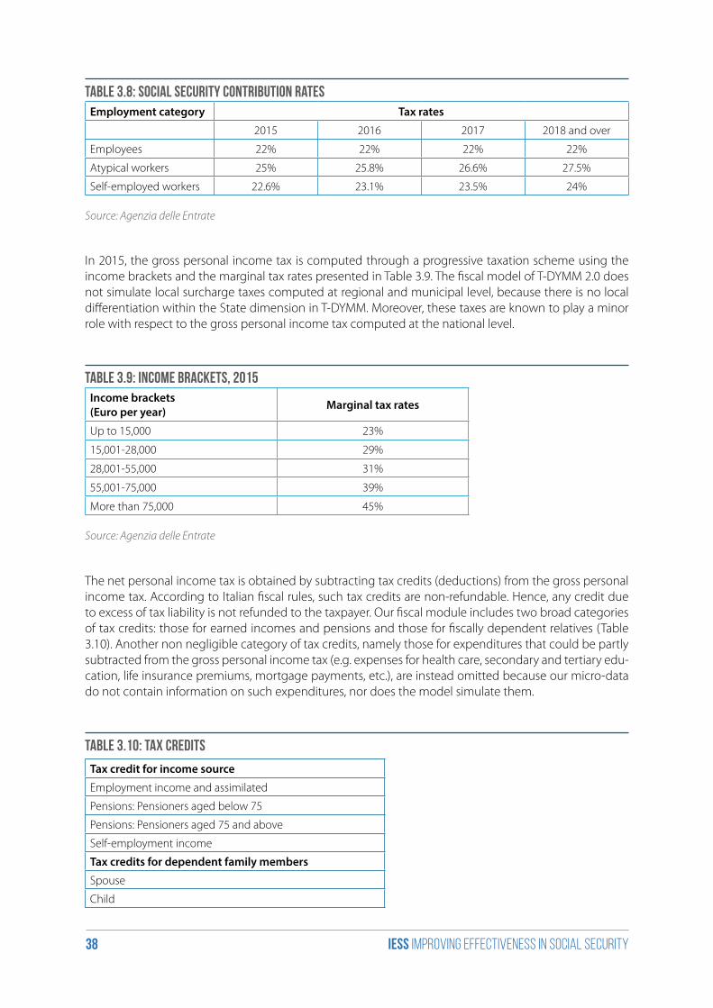
iess Improving effectiveness in social security38
Table 3.8: Social security contribution ratesEmployment category Tax rates
2015 2016 2017 2018 and over
Employees 22% 22% 22% 22%
Atypical workers 25% 25.8% 26.6% 27.5%
Self-employed workers 22.6% 23.1% 23.5% 24%
Source: Agenzia delle Entrate
In 2015, the gross personal income tax is computed through a progressive taxation scheme using the income brackets and the marginal tax rates presented in Table 3.9. The fiscal model of T-DYMM 2.0 does not simulate local surcharge taxes computed at regional and municipal level, because there is no local differentiation within the State dimension in T-DYMM. Moreover, these taxes are known to play a minor role with respect to the gross personal income tax computed at the national level.
Table 3.9: Income brackets, 2015Income brackets(Euro per year) Marginal tax rates
Up to 15,000 23%
15,001-28,000 29%
28,001-55,000 31%
55,001-75,000 39%
More than 75,000 45%
Source: Agenzia delle Entrate
The net personal income tax is obtained by subtracting tax credits (deductions) from the gross personal income tax. According to Italian fiscal rules, such tax credits are non-refundable. Hence, any credit due to excess of tax liability is not refunded to the taxpayer. Our fiscal module includes two broad categories of tax credits: those for earned incomes and pensions and those for fiscally dependent relatives (Table 3.10). Another non negligible category of tax credits, namely those for expenditures that could be partly subtracted from the gross personal income tax (e.g. expenses for health care, secondary and tertiary edu-cation, life insurance premiums, mortgage payments, etc.), are instead omitted because our micro-data do not contain information on such expenditures, nor does the model simulate them.
Table 3.10: Tax credits
Tax credit for income source
Employment income and assimilated
Pensions: Pensioners aged below 75
Pensions: Pensioners aged 75 and above
Self-employment income
Tax credits for dependent family members
Spouse
Child
iess Improving effectiveness in social security39
References
Dekkers, G., Buslei H., Cozzolino M., Desmet R., Geyer J., Hofmann D., Raitano M., Steiner V., Tanda P., Tede-schi S., Verschueren F. (2009). What Are the Consequences of AWG Projections for the Adequacy of Social Security Pensions? ENEPRI Research Report N. 65, AIM WP4;
European Commission - Directorate-General for Economic and Financial Affairs - The 2015 Ageing Re-port: Economic and budgetary projections for the EU28 Member States (2013-2060);
O’Donoghue, C. (2001), “Dynamic Microsimulation: A Methodological Survey”, Brazilian Electronic Jour-nal of Economics, Universidade Federal de Pernambuco, vol. 4, n.2.
iess Improving effectiveness in social security40
4. The estimations employed in the modules
As widely analysed in chapter 1, the first innovation of T-DYMM 2.0 is the use of a new and improved dataset for the estimations imported in the microsimulation model.
Because of the existence of a panel dimension not only on the administrative side, but also in the SILC portion of the dataset, T-DYMM 2.0 can make use of more solid estimations compared to the ones cha-racterising the first version of the model for the purpose of the labour market module. Moreover, for what concerns the demographic module, T-DYMM 2.0 has now departed from MIDAS-IT and employs autonomous estimation on a number of demographic variables. As a complete innovation from T-DYMM 1.0, T-DYMM 2.0 also makes use of the panel information collected in SILC to estimate the probability of contributing to occupational and individual pension plans.
It should be noted that – and this is true for all estimations which parameters are imported in the model – not all of the variables present in AD-SILC dataset can effectively be utilised in the estimation phase. Specifically, we do not include in our regressions any variable that is not present in the “simulation world” because of the impracticability of projecting its evolution in time. For instance, while the dimension of the firm may have relevance in explaining the probability of a worker to contribute to occupational pension plans, we do not differentiate by firm dimension in the model and we have excluded this para-meter from the external estimations, because we find it unfeasible to project whether workers will keep working for a specific type of firm.
We are aware that omitted variables may distort some of the estimated coefficients. Nonetheless, other than the impact of time dummies, we decided to maintain our coefficients unaffected in order to mini-mize the loss of valuable information and to avoid counterintuitive results.
A series of regressions has been carried out for the purpose, employing various explanatory variables. We give a brief description of them, as follows:
• age and age2 – age and the relative quadratic form;
• age25-29, age30-34,..,age_over49,… – dummies for 5-year age classes; the first age class comprise individuals aged 25-29 years and the last individuals age 49 years or more;
• upsec and univ – dummies indicating the education level ( upper-secondary and university), the reference category being an educational attainment below upper secondary degree;
• marr –a dummy for being married or cohabiting rather than single/separated/divorced or widow;
• single/divorced/widowed– dummy for being single/divorced/widowed rather than married/coha-biting;
• agediff, agediff2 and agediff3 – the difference between the women’s age and the average age of their male counterparts, its quadratic and cubic form;
• p_age, p_age2 and p_age3 – the age of the partner and its quadratic and cubic form;
• pareduach– parental education (see Table 4.2);
• edudiff_0 and edudiff_1 –dummies for the difference in the education level between the two spou-

iess Improving effectiveness in social security41
ses: the first indicates no difference in the education and the second 1-level difference (the reference group for the two dummies is couples with education difference greater than 1);
• dur_marriageand dur_marriage2– years of marriage and its quadratic form;
• dummy_numch1 – dummy equal to 1 if children are 1 year old;
• numch03, etc. – the number of children in different age bands, depending on the level of significan-ce of the groups (0-3, pre-school age; 0-11, pre-school and primary school age; 4-11, primary school age; 12-15, lower-secondary school age);
• potexp and potexp2 – the accrued work experience, as computed by the years spent working in the AD-SILC panel, and its quadratic;
• inwork_1 – dummy for being employed at time t-1;
• p_inworkand p_inwork_1 – the employment condition of the spouse/partner respectively at time t and t-1, for those who are married/cohabiting;
• dummies capturing several work conditions at time t-1 when the option lag is included, namely:
-dip_1, coco_1, aut_1 – whether the individual is an employee, a parasubordinate worker, or self-employed, whereas the reference group is not employed in t-1;
-public, pt, perm –when in work as an employee, whether the individual is working in the public or private sector; part-time or full-time; has a permanent or temporary contract. when the option lag is included then we have public_1, pt_1, perm_1
• p_public_1andp_perm_1– dummies for having a partner working, respectively, as public and per-manent employee at time t-1;
• duration, expressed in levels, and its quadratic; these variables refer to the work condition at time t-1, and therefore:
-durwork_1 and durwork2 – the number of consecutive years spent in formal employment up to time t-1 and its quadratic in the equation predicting the chances of being in work;
-durdip_1 and durdip2, durcoco_1 and durcoco2, duraut_1 and duraut2 –the number of con-secutive years as an employee/parasubordinate/self-employed up to time t-1 and the respective quadratic forms;
-durpub_1anddurpub2,durperm_1anddurperm2, durpt_1anddurpt2 – the number of con-secutive years as a public/permanent/part-time employee up to time t-1 and the respective qua-dratic forms;
• inw_allyr and inw_allyr_1 – dummies for having been in work all year at time t and t-1, respectively;
• cococo – dummy for being an atypical worker rather than a temporary employee;
• pensit and pensit_1 – dummy equal to 1 when individuals are enrolled in “individual” pension funds, at time t and t-1, respectively;
• convol_1 - dummy equal to 1 when individuals are enrolled in “collective” pension funds, at time t and t-1, respectively;
• logwage – logarithm of wages (2011 nominal value).
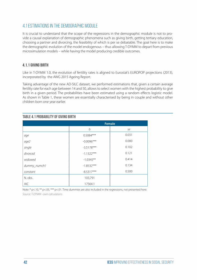
iess Improving effectiveness in social security42
4.1 Estimations in the demographic module
It is crucial to understand that the scope of the regressions in the demographic module is not to pro-vide a causal explanation of demographic phenomena such as giving birth, getting tertiary education, choosing a partner and divorcing, the feasibility of which is per se debatable. The goal here is to make the demographic evolution of the model endogenous – thus allowing T-DYMM to depart from previous microsimulation models – while having the model producing credible outcomes.
4.1.1 Giving birth
Like in T-DYMM 1.0, the evolution of fertility rates is aligned to Eurostat’s EUROPOP projections (2013), incorporated by the AWG 2015 Ageing Report.
Taking advantage of the new AD-SILC dataset, we performed estimations that, given a certain average fertility rate for each age between 14 and 50, allows to select women with the highest probability to give birth in a given period. The probabilities have been estimated using a random effects logistic model. As shown in Table 1, these women are essentially characterised by being in couple and without other children born one year earlier.
Table 4.1 Probability of giving birth
Female
b se
age 0.5084*** 0.031
age2 -0.0096*** 0.000
single -3.5178*** 0.102
divorced -1.1322*** 0.121
widowed -1.0345** 0.414
dummy_numch1 -1.8532*** 0.134
constant -8.5317*** 0.500
N. obs. 103,791
AIC 17564.1
Note: * p<.10, ** p<.05, *** p<.01. Time dummies are also included in the regressions, not presented here.
Source: T-DYMM - own calculations
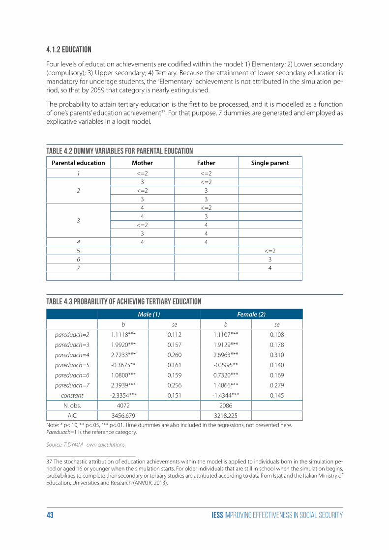
iess Improving effectiveness in social security43
4.1.2 Education
Four levels of education achievements are codified within the model: 1) Elementary; 2) Lower secondary (compulsory); 3) Upper secondary; 4) Tertiary. Because the attainment of lower secondary education is mandatory for underage students, the “Elementary” achievement is not attributed in the simulation pe-riod, so that by 2059 that category is nearly extinguished.
The probability to attain tertiary education is the first to be processed, and it is modelled as a function of one’s parents’ education achievement37. For that purpose, 7 dummies are generated and employed as explicative variables in a logit model.
Table 4.2 Dummy variables for parental educationParental education Mother Father Single parent
1 <=2 <=2
23 <=2
<=2 33 3
3
4 <=24 3
<=2 43 4
4 4 45 <=26 37 4
Table 4.3 Probability of achieving tertiary education
Male(1) Female(2)
b se b se
pareduach=2 1.1118*** 0.112 1.1107*** 0.108
pareduach=3 1.9920*** 0.157 1.9129*** 0.178
pareduach=4 2.7233*** 0.260 2.6963*** 0.310
pareduach=5 -0.3675** 0.161 -0.2995** 0.140
pareduach=6 1.0800*** 0.159 0.7320*** 0.169
pareduach=7 2.3939*** 0.256 1.4866*** 0.279
constant -2.3354*** 0.151 -1.4344*** 0.145
N. obs. 4072 2086
AIC 3456.679 3218.225Note: * p<.10, ** p<.05, *** p<.01. Time dummies are also included in the regressions, not presented here.Pareduach=1 is the reference category.
Source: T-DYMM - own calculations
37 The stochastic attribution of education achievements within the model is applied to individuals born in the simulation pe-riod or aged 16 or younger when the simulation starts. For older individuals that are still in school when the simulation begins, probabilities to complete their secondary or tertiary studies are attributed according to data from Istat and the Italian Ministry of Education, Universities and Research (ANVUR, 2013).
iess Improving effectiveness in social security44
The amount of individuals attaining tertiary education is aligned to probabilities extracted by Istat data. Such amount evolves in the simulation period by means of a logarithmic scale. Because of it, the share of individuals aged between 30 and 34 holding a university degree raises from 25.2% in 2012 to 28.7% in 2059, passing the Europe 2020 goal of 27% by 2040. The share of women holding tertiary education is 10 percentage points higher than that of men over the historical sample. By assumption, this feature is kept constant throughout the whole simulation period.
If individuals are assigned a tertiary education achievement, a random process determines at what age they exit the education module and access the labour model38.
If individuals are not assigned a tertiary education achievement, a random process assigns them either lower or upper secondary education, according to probabilities that evolve in the simulation period by means of a logarithmic scale.
The transition from education to work is irreversible and student-workers are not simulated in T-DYMM at this time.
4.1.3 Marriage market
In accordance with the procedure proposed by LIAM2 developers, the coupling process is articulated in three steps:
1. Individuals (male and female) to be coupled are selected amongst all singles aged between 18 and 65 via a logit regression (we have employed a random effects logistic model);
2. The selected females are ordered by the difference between their own age and the average age of their male counterparts (the oldest females get the highest scores, so that they are sure to be se-lected first);
3. The selected males are ordered by means of a score, estimated with a logit regression.
An alignment process is implemented with the scope of maintaining an equal share of coupled adults in the simulation period. Because of the fact that no difference could be observed in the AD-SILC data-set between married and cohabiting couples, those processes are not dealt with separately39. Instead, a portion of the newly coupled individuals are assigned to marriage every year. We have implemented an alignment procedure that, with the use of a logarithmic function, predicts the evolution of the quota of marriages on overall unions, thus depicting the decreasing trend in marriages observed in the past 20 years (Istat)40.
For the purpose of selecting individuals to be coupled, the parameters in table 4 are imported in the model.
38 Data from Almalaurea.39 It is however of some relevance to treat married couples separately. For what concerns labor choices, it is conceivable that a legal commitment impacts such decisions, and we have verified that it does in our labor market estimations (see further). For what concerns pensions, married couples are the ones who can access survivor’s pensions.
It is also relevant to keep cohabiting individuals into consideration, mainly for what concerns the “giving birth” process.40 However, the quota of married couples on overall couples decreases very slightly in the simulation period, from 92.93% in 2011 to 90.26% in 2059.
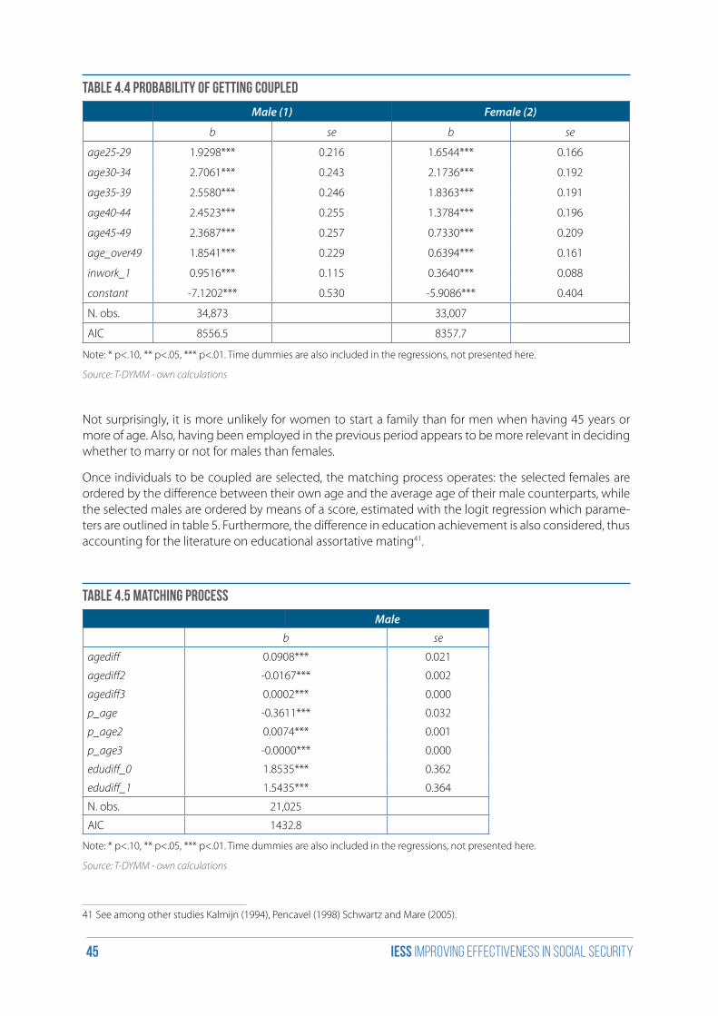
iess Improving effectiveness in social security45
Table 4.4 Probability of getting coupled
Male(1) Female(2)
b se b se
age25-29 1.9298*** 0.216 1.6544*** 0.166
age30-34 2.7061*** 0.243 2.1736*** 0.192
age35-39 2.5580*** 0.246 1.8363*** 0.191
age40-44 2.4523*** 0.255 1.3784*** 0.196
age45-49 2.3687*** 0.257 0.7330*** 0.209
age_over49 1.8541*** 0.229 0.6394*** 0.161
inwork_1 0.9516*** 0.115 0.3640*** 0.088
constant -7.1202*** 0.530 -5.9086*** 0.404
N. obs. 34,873 33,007
AIC 8556.5 8357.7
Note: * p<.10, ** p<.05, *** p<.01. Time dummies are also included in the regressions, not presented here.
Source: T-DYMM - own calculations
Not surprisingly, it is more unlikely for women to start a family than for men when having 45 years or more of age. Also, having been employed in the previous period appears to be more relevant in deciding whether to marry or not for males than females.
Once individuals to be coupled are selected, the matching process operates: the selected females are ordered by the difference between their own age and the average age of their male counterparts, while the selected males are ordered by means of a score, estimated with the logit regression which parame-ters are outlined in table 5. Furthermore, the difference in education achievement is also considered, thus accounting for the literature on educational assortative mating41.
Table 4.5 Matching process
Male
b se
agediff 0.0908*** 0.021
agediff2 -0.0167*** 0.002
agediff3 0.0002*** 0.000
p_age -0.3611*** 0.032
p_age2 0.0074*** 0.001
p_age3 -0.0000*** 0.000
edudiff_0 1.8535*** 0.362
edudiff_1 1.5435*** 0.364
N. obs. 21,025
AIC 1432.8
Note: * p<.10, ** p<.05, *** p<.01. Time dummies are also included in the regressions, not presented here.
Source: T-DYMM - own calculations
41 See among other studies Kalmijn (1994), Pencavel (1998) Schwartz and Mare (2005).
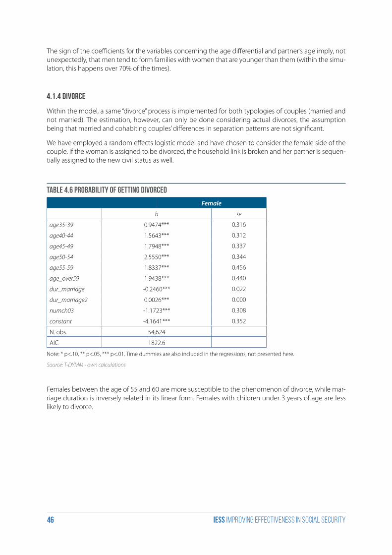
iess Improving effectiveness in social security46
The sign of the coefficients for the variables concerning the age differential and partner’s age imply, not unexpectedly, that men tend to form families with women that are younger than them (within the simu-lation, this happens over 70% of the times).
4.1.4 Divorce
Within the model, a same “divorce” process is implemented for both typologies of couples (married and not married). The estimation, however, can only be done considering actual divorces, the assumption being that married and cohabiting couples’ differences in separation patterns are not significant.
We have employed a random effects logistic model and have chosen to consider the female side of the couple. If the woman is assigned to be divorced, the household link is broken and her partner is sequen-tially assigned to the new civil status as well.
Table 4.6 Probability of getting divorced
Female
b se
age35-39 0.9474*** 0.316
age40-44 1.5643*** 0.312
age45-49 1.7948*** 0.337
age50-54 2.5550*** 0.344
age55-59 1.8337*** 0.456
age_over59 1.9438*** 0.440
dur_marriage -0.2460*** 0.022
dur_marriage2 0.0026*** 0.000
numch03 -1.1723*** 0.308
constant -4.1641*** 0.352
N. obs. 54,624
AIC 1822.6
Note: * p<.10, ** p<.05, *** p<.01. Time dummies are also included in the regressions, not presented here.
Source: T-DYMM - own calculations
Females between the age of 55 and 60 are more susceptible to the phenomenon of divorce, while mar-riage duration is inversely related in its linear form. Females with children under 3 years of age are less likely to divorce.
iess Improving effectiveness in social security47
4.2 Estimations in the labour market module
A crucial step in building the labour market module is the estimation of conditional probabilities of tran-sition across alternative employment states42.
First, as explained in section 3, we estimate the conditional probability to be employed thus determining who is actually employed and then assign as not employed the rest of the working age population. Once the individual has been included in the labour market as employed it is necessary to determine whether he/she is an employee, or independent worker. Differently from the previous version of T-DYMM, here the first work choice is ascribed to the parasubordinate status (registered in Gestione Separata of INPS). The rationale behind this choice is that parasubordinate workers represent a particular category of the Italian labour market and we need to define a share that suitably reflects the employment composition as it is in the labour market. Starting with the estimation of the probability of ending up in the parasubordinate state allows to set up its share and thus to prevent the risk of extremely reducing it in the upcoming ye-ars. If the worker is not assigned to this work state the propensity of being an employee is determined. This is the prevalent category and the probability that a worker becomes an employee is far greater than those of the other two states, therefore there is no need to do further adjustments. If the worker does not go into this status either, then he/she is assigned to the self-employed state which represents a residual category. The need of decomposing the employment in these three states is due to the fact that they implicate different career paths as well as different pension schemes and contributions.
Second, once an individual is assigned the status of employee, the subsequent choices concern the type of economic activity (private or public); duration of contract (permanent or temporary); and working time arrangements (full-time or part-time). These job characteristics exert an impact both on the proba-bility of transition across employment states, and on the level of earnings.
Finally, once the working condition has been determined, the following step is the simulation of months worked and a yearly labour income, gross of personal income taxation; this is exactly the measure of ear-nings that represents the base on which contribution rates have to be applied in order to calculate the contribution to future pension benefits.
4.2.1 Transitions among employment states
This section presents the estimation results of the regressions of the employment transitions, whereas the estimated parameters are used in the T-DYMM model to simulate the labour market conditions. The entire AD-SILC dataset is used for the estimation (e.g. all IT-SILC waves merged with the INPS archives). As long as INPS considers only statuses of individuals paying contributions we are not able to infer why individuals are recorded in some years and not present in others, i.e. we cannot ascertain whether their absence from administrative records is due to exit from the labour force for unemployment without being entitled to benefits, entry in the shadow economy, discouragement, and so on. Therefore, those individuals that are not assigned to any employment status are considered as inactive43.
42 A detailed description of the labour market module is presented in section 3.2.2.43 As far as our purpose is to study the contribution accumulation of different working career patterns and the redistributive effects of the Italian pension system and given that an individual working in the shadow economy by definition does not pay any contributions, it is not of a great concern that this individual is assigned as inactive rather than as a worker with undeclared job relationship. The drawbacks come up if one wants to study in-depth the labour market dynamics.
iess Improving effectiveness in social security48
The sample size amounts to 1,105,456 observations for 82,137 individuals, followed over the time span 1998-2011. We focus on individuals aged 16-69, whereas almost 53 percent are men and the rest 47 per-cent women. Behavioural equations are estimated using random effects logistic models44 separately for men and women.
As in most MSMs, it is assumed that the characteristics of the employment are ‘decided’ by the individual, and therefore do not depend on demand-side factors.
a) Employment
The first event simulated in the labour market module is employment. This is modelled separately for males and females, and the reference group is all individuals aged 16-69 who were employed or not in education nor retired at time t-145. The resulting employment rates are then aligned with gender and age-group specific of the AWG 2015 Ageing Report projections (with the first years of simulation adju-sted using the actual figures from Eurostat). This implies a two-step procedure; in the first step, indivi-duals are ranked according to decreasing propensity to the event (here, probability of being in formal employment), depending on their characteristics; once this ranking is built, by using the regressions re-ported below, the number of individuals simulated as actually being in work is established so that the re-sulting employment rates are consistent with the alignment data; for each gender/age group subgroup, n individuals will be imputed an in-work status, and these will be persons in the top n positions in the ranking.
Table 4.7 reports the estimated parameters for the regression concerning the probability of being em-ployed, both for men and women. Regardless the gender, the higher the education level the higher the probability of being employed. There are more chances to be employed with the increase of age and the overall work experience albeit at decreasing rates. Similarly, more years the individual has been employed without spells the higher the probability of being in work also at time t. Being employed in t-1 increases the likelihood of being it again whereas employees and self-employed (at time t-1) are more advantaged than atypical workers.
Also, factors related to family background appear to be relevant for women; being married/cohabiting and the number of children up to 11 years of age reduce the chances of a woman to maintain her em-ployment. Yet, having a spouse in work rises her likelihood to work, too.
44 In the previous project two procedures have been employed: random effects logistic models whenever the sample size was large enough and simple logistic regressions in all the other cases. In particular, given the relatively small sample size of the old version of AD-SILC the first type of regressions has been used only to estimate the probabilities of being in work having been in work in the previous year, and the probability of being an employee having been an employee at time t-1 as well. The new AD-SILC is almost four times larger than its old version (that used in the previous project) which allows to apply the same regression technique for all employment states. 45 We recall that education, employment and retirement are three mutually exclusive states in the model.
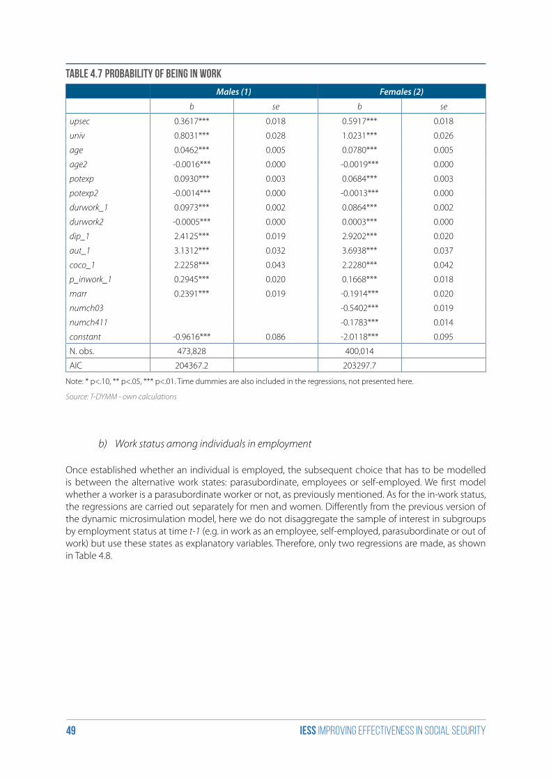
iess Improving effectiveness in social security49
Table 4.7 Probability of being in work
Males(1) Females(2)
b se b se
upsec 0.3617*** 0.018 0.5917*** 0.018
univ 0.8031*** 0.028 1.0231*** 0.026
age 0.0462*** 0.005 0.0780*** 0.005
age2 -0.0016*** 0.000 -0.0019*** 0.000
potexp 0.0930*** 0.003 0.0684*** 0.003
potexp2 -0.0014*** 0.000 -0.0013*** 0.000
durwork_1 0.0973*** 0.002 0.0864*** 0.002
durwork2 -0.0005*** 0.000 0.0003*** 0.000
dip_1 2.4125*** 0.019 2.9202*** 0.020
aut_1 3.1312*** 0.032 3.6938*** 0.037
coco_1 2.2258*** 0.043 2.2280*** 0.042
p_inwork_1 0.2945*** 0.020 0.1668*** 0.018
marr 0.2391*** 0.019 -0.1914*** 0.020
numch03 -0.5402*** 0.019
numch411 -0.1783*** 0.014
constant -0.9616*** 0.086 -2.0118*** 0.095
N. obs. 473,828 400,014
AIC 204367.2 203297.7
Note: * p<.10, ** p<.05, *** p<.01. Time dummies are also included in the regressions, not presented here.
Source: T-DYMM - own calculations
b) Work status among individuals in employment
Once established whether an individual is employed, the subsequent choice that has to be modelled is between the alternative work states: parasubordinate, employees or self-employed. We first model whether a worker is a parasubordinate worker or not, as previously mentioned. As for the in-work status, the regressions are carried out separately for men and women. Differently from the previous version of the dynamic microsimulation model, here we do not disaggregate the sample of interest in subgroups by employment status at time t-1 (e.g. in work as an employee, self-employed, parasubordinate or out of work) but use these states as explanatory variables. Therefore, only two regressions are made, as shown in Table 4.8.
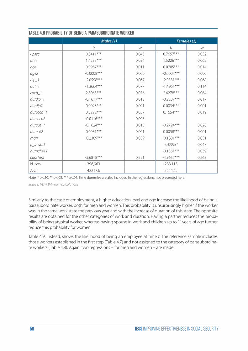
iess Improving effectiveness in social security50
Table 4.8 Probability of being a parasubordinate worker
Males(1) Females(2)
b se b se
upsec 0.8411*** 0.043 0.7657*** 0.052
univ 1.4255*** 0.054 1.5226*** 0.062
age 0.0967*** 0.011 0.0705*** 0.014
age2 -0.0008*** 0.000 -0.0007*** 0.000
dip_1 -2.0598*** 0.067 -2.0331*** 0.068
aut_1 -1.3664*** 0.077 -1.4964*** 0.114
coco_1 2.8063*** 0.076 2.4278*** 0.064
durdip_1 -0.1617*** 0.013 -0.2207*** 0.017
durdip2 0.0023*** 0.001 0.0034*** 0.001
durcoco_1 0.3222*** 0.037 0.1654*** 0.019
durcoco2 -0.0116*** 0.003
duraut_1 -0.1624*** 0.015 -0.2724*** 0.028
duraut2 0.0031*** 0.001 0.0058*** 0.001
marr -0.2389*** 0.039 -0.1801*** 0.051
p_inwork -0.0995* 0.047
numch411 -0.1361*** 0.039
constant -5.6818*** 0.221 -4.9657*** 0.263
N. obs. 396,963 288,113
AIC 42217.6 35442.5
Note: * p<.10, ** p<.05, *** p<.01. Time dummies are also included in the regressions, not presented here.
Source: T-DYMM - own calculations
Similarly to the case of employment, a higher education level and age increase the likelihood of being a parasubordinate worker, both for men and women. This probability is unsurprisingly higher if the worker was in the same work state the previous year and with the increase of duration of this state. The opposite results are obtained for the other categories of work and duration. Having a partner reduces the proba-bility of being atypical worker, whereas having spouse in work and children up to 11years of age further reduce this probability for women.
Table 4.9, instead, shows the likelihood of being an employee at time t. The reference sample includes those workers established in the first step (Table 4.7) and not assigned to the category of parasubordina-te workers (Table 4.8). Again, two regressions – for men and women – are made.
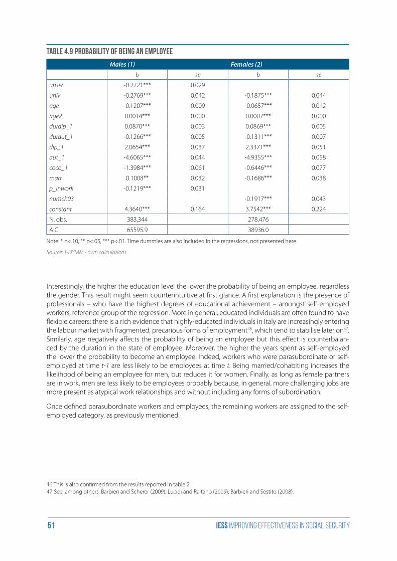
iess Improving effectiveness in social security51
Table 4.9 Probability of being an employee
Males(1) Females(2)
b se b se
upsec -0.2721*** 0.029
univ -0.2769*** 0.042 -0.1875*** 0.044
age -0.1207*** 0.009 -0.0657*** 0.012
age2 0.0014*** 0.000 0.0007*** 0.000
durdip_1 0.0870*** 0.003 0.0869*** 0.005
duraut_1 -0.1266*** 0.005 -0.1311*** 0.007
dip_1 2.0654*** 0.037 2.3371*** 0.051
aut_1 -4.6065*** 0.044 -4.9355*** 0.058
coco_1 -1.3984*** 0.061 -0.6446*** 0.077
marr 0.1008** 0.032 -0.1686*** 0.038
p_inwork -0.1219*** 0.031
numch03 -0.1917*** 0.043
constant 4.3640*** 0.164 3.7542*** 0.224
N. obs. 383,344 278,476
AIC 65595.9 38936.0
Note: * p<.10, ** p<.05, *** p<.01. Time dummies are also included in the regressions, not presented here.
Source: T-DYMM - own calculations
Interestingly, the higher the education level the lower the probability of being an employee, regardless the gender. This result might seem counterintuitive at first glance. A first explanation is the presence of professionals – who have the highest degrees of educational achievement – amongst self-employed workers, reference group of the regression. More in general, educated individuals are often found to have flexible careers: there is a rich evidence that highly-educated individuals in Italy are increasingly entering the labour market with fragmented, precarious forms of employment46, which tend to stabilise later on47. Similarly, age negatively affects the probability of being an employee but this effect is counterbalan-ced by the duration in the state of employee. Moreover, the higher the years spent as self-employed the lower the probability to become an employee. Indeed, workers who were parasubordinate or self-employed at time t-1 are less likely to be employees at time t. Being married/cohabiting increases the likelihood of being an employee for men, but reduces it for women. Finally, as long as female partners are in work, men are less likely to be employees probably because, in general, more challenging jobs are more present as atypical work relationships and without including any forms of subordination.
Once defined parasubordinate workers and employees, the remaining workers are assigned to the self-employed category, as previously mentioned.
46 This is also confirmed from the results reported in table 2.47 See, among others, Barbieri and Scherer (2009); Lucidi and Raitano (2009); Barbieri and Sestito (2008).
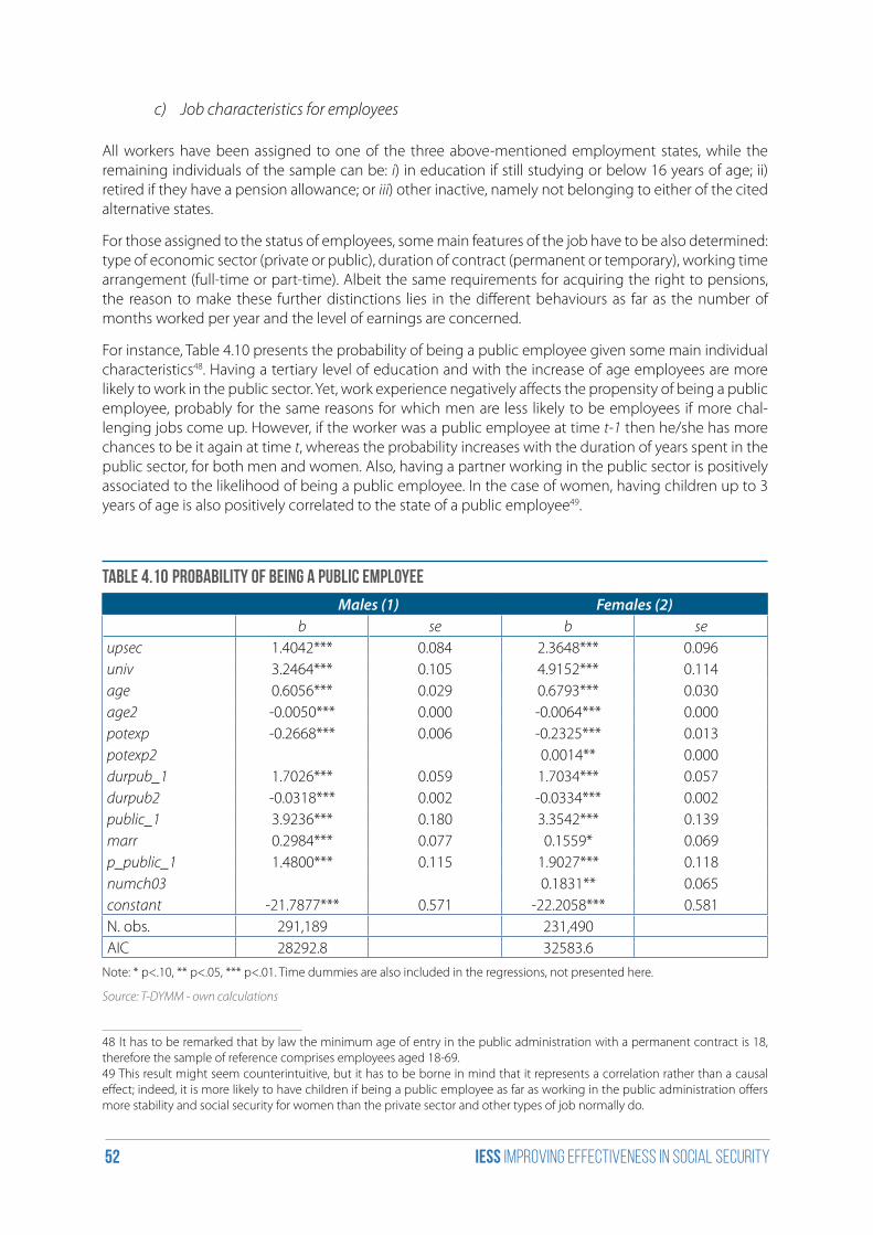
iess Improving effectiveness in social security52
c) Job characteristics for employees
All workers have been assigned to one of the three above-mentioned employment states, while the remaining individuals of the sample can be: i) in education if still studying or below 16 years of age; ii) retired if they have a pension allowance; or iii) other inactive, namely not belonging to either of the cited alternative states.
For those assigned to the status of employees, some main features of the job have to be also determined: type of economic sector (private or public), duration of contract (permanent or temporary), working time arrangement (full-time or part-time). Albeit the same requirements for acquiring the right to pensions, the reason to make these further distinctions lies in the different behaviours as far as the number of months worked per year and the level of earnings are concerned.
For instance, Table 4.10 presents the probability of being a public employee given some main individual characteristics48. Having a tertiary level of education and with the increase of age employees are more likely to work in the public sector. Yet, work experience negatively affects the propensity of being a public employee, probably for the same reasons for which men are less likely to be employees if more chal-lenging jobs come up. However, if the worker was a public employee at time t-1 then he/she has more chances to be it again at time t, whereas the probability increases with the duration of years spent in the public sector, for both men and women. Also, having a partner working in the public sector is positively associated to the likelihood of being a public employee. In the case of women, having children up to 3 years of age is also positively correlated to the state of a public employee49.
Table 4.10 Probability of being a public employee
Males(1) Females(2)b se b se
upsec 1.4042*** 0.084 2.3648*** 0.096univ 3.2464*** 0.105 4.9152*** 0.114age 0.6056*** 0.029 0.6793*** 0.030age2 -0.0050*** 0.000 -0.0064*** 0.000potexp -0.2668*** 0.006 -0.2325*** 0.013potexp2 0.0014** 0.000durpub_1 1.7026*** 0.059 1.7034*** 0.057durpub2 -0.0318*** 0.002 -0.0334*** 0.002public_1 3.9236*** 0.180 3.3542*** 0.139marr 0.2984*** 0.077 0.1559* 0.069p_public_1 1.4800*** 0.115 1.9027*** 0.118numch03 0.1831** 0.065constant -21.7877*** 0.571 -22.2058*** 0.581N. obs. 291,189 231,490AIC 28292.8 32583.6
Note: * p<.10, ** p<.05, *** p<.01. Time dummies are also included in the regressions, not presented here.
Source: T-DYMM - own calculations
48 It has to be remarked that by law the minimum age of entry in the public administration with a permanent contract is 18, therefore the sample of reference comprises employees aged 18-69.49 This result might seem counterintuitive, but it has to be borne in mind that it represents a correlation rather than a causal effect; indeed, it is more likely to have children if being a public employee as far as working in the public administration offers more stability and social security for women than the private sector and other types of job normally do.
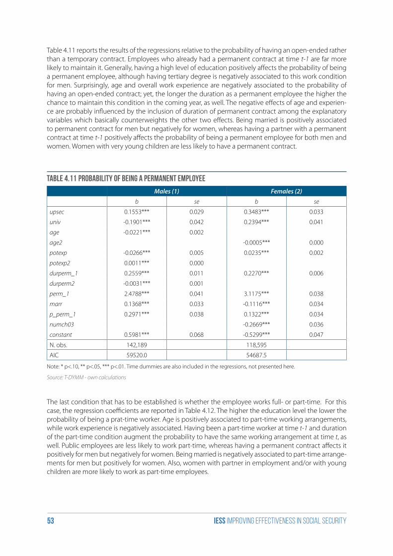
iess Improving effectiveness in social security53
Table 4.11 reports the results of the regressions relative to the probability of having an open-ended rather than a temporary contract. Employees who already had a permanent contract at time t-1 are far more likely to maintain it. Generally, having a high level of education positively affects the probability of being a permanent employee, although having tertiary degree is negatively associated to this work condition for men. Surprisingly, age and overall work experience are negatively associated to the probability of having an open-ended contract; yet, the longer the duration as a permanent employee the higher the chance to maintain this condition in the coming year, as well. The negative effects of age and experien-ce are probably influenced by the inclusion of duration of permanent contract among the explanatory variables which basically counterweights the other two effects. Being married is positively associated to permanent contract for men but negatively for women, whereas having a partner with a permanent contract at time t-1 positively affects the probability of being a permanent employee for both men and women. Women with very young children are less likely to have a permanent contract.
Table 4.11 Probability of being a permanent employee
Males(1) Females(2)
b se b se
upsec 0.1553*** 0.029 0.3483*** 0.033
univ -0.1901*** 0.042 0.2394*** 0.041
age -0.0221*** 0.002
age2 -0.0005*** 0.000
potexp -0.0266*** 0.005 0.0235*** 0.002
potexp2 0.0011*** 0.000
durperm_1 0.2559*** 0.011 0.2270*** 0.006
durperm2 -0.0031*** 0.001
perm_1 2.4788*** 0.041 3.1175*** 0.038
marr 0.1368*** 0.033 -0.1116*** 0.034
p_perm_1 0.2971*** 0.038 0.1322*** 0.034
numch03 -0.2669*** 0.036
constant 0.5981*** 0.068 -0.5299*** 0.047
N. obs. 142,189 118,595
AIC 59520.0 54687.5
Note: * p<.10, ** p<.05, *** p<.01. Time dummies are also included in the regressions, not presented here.
Source: T-DYMM - own calculations
The last condition that has to be established is whether the employee works full- or part-time. For this case, the regression coefficients are reported in Table 4.12. The higher the education level the lower the probability of being a prat-time worker. Age is positively associated to part-time working arrangements, while work experience is negatively associated. Having been a part-time worker at time t-1 and duration of the part-time condition augment the probability to have the same working arrangement at time t, as well. Public employees are less likely to work part-time, whereas having a permanent contract affects it positively for men but negatively for women. Being married is negatively associated to part-time arrange-ments for men but positively for women. Also, women with partner in employment and/or with young children are more likely to work as part-time employees.
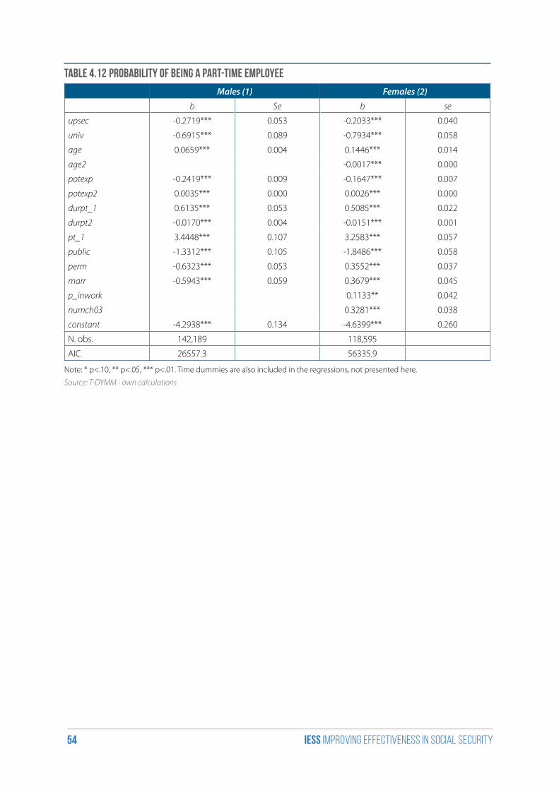
iess Improving effectiveness in social security54
Table 4.12 Probability of being a part-time employee
Males(1) Females(2)
b Se b se
upsec -0.2719*** 0.053 -0.2033*** 0.040
univ -0.6915*** 0.089 -0.7934*** 0.058
age 0.0659*** 0.004 0.1446*** 0.014
age2 -0.0017*** 0.000
potexp -0.2419*** 0.009 -0.1647*** 0.007
potexp2 0.0035*** 0.000 0.0026*** 0.000
durpt_1 0.6135*** 0.053 0.5085*** 0.022
durpt2 -0.0170*** 0.004 -0.0151*** 0.001
pt_1 3.4448*** 0.107 3.2583*** 0.057
public -1.3312*** 0.105 -1.8486*** 0.058
perm -0.6323*** 0.053 0.3552*** 0.037
marr -0.5943*** 0.059 0.3679*** 0.045
p_inwork 0.1133** 0.042
numch03 0.3281*** 0.038
constant -4.2938*** 0.134 -4.6399*** 0.260
N. obs. 142,189 118,595
AIC 26557.3 56335.9
Note: * p<.10, ** p<.05, *** p<.01. Time dummies are also included in the regressions, not presented here.
Source: T-DYMM - own calculations
iess Improving effectiveness in social security55
4.2.2 Estimating gross earnings and months worked
Yearly individual labour income gross of personal income taxation is the product of two components: monthly gross income and months worked.
a) Monthly earnings
In order to estimate the first component, separately for the three main typologies of workers as well as for men and women, accounting for individual unobserved heterogeneity, we use a Fixed Effect (FE) estimator on the retrospective AD-SILC panel50. In the simulation program we use actual predicted values of fixed effect for in sample individuals, while for new-born or out-of-sample individuals we impute this value as a random draw from a normal distribution with the estimated standard deviation. Since each individual can potentially be employed in more than one category over the life cycle, he/she must be endowed with a three dimensional residual fixed effect, one for each work category. We assume that the value for this residual is perfectly correlated to the value in the prevalent states. In other words, for out-of-sample individuals, the residual FE is a random draw from a three-variate normal distribution with correlation coefficient equal to one. The rationale behind this assumption relies on the fact that unobserved time-invariant heterogeneity typically accounts for ability or soft skills or other characteri-stics which make the individual constantly above or below the average. Therefore, we consider a sensible assumption that such relative position persists across work typologies as well.
Estimates are carried out using an AD-SILC sample composed of 1,282,863 observations for 102,865 in-dividuals, once again followed over the time span 1998-2011. Regressions are carried out separately for men and women, and for the three main work categories modelled in T-DYMM. In the retrospective panel the work typology of a formally employed individual was established mainly according to the prevalence of earnings from one of the three work categories. It should be noted, however, that once a worker is assigned to a category in a given year, the overall income he/she earned over that period is attributed to that category. In other words, even if an individual earned a part of his/her labour income from a different typology of work, when estimating earnings equations the sum of incomes from all typologies is used as the dependent variable. Since the model excludes the possibility of a worker having more than one job or type of job over a year, this was the only way to avoid an underestimation of yearly labour incomes.
The dependent variable is the logarithm of monthly gross earnings51; these are clearly an average of annual earnings, computed as the ratio between overall labour income earned over the year and the number of months worked over the period. It should be noticed that this measure of time spent in employment is not based on the actual duration of a contract, but rather on the number of weeks of contribution to pension funds, as the latter is the relevant information as far as the accumulation of pension contributions is concerned.
50 To account for the role of time invariant observed characteristics, which is prevented when using a FE estimate, in the previ-ous version of T-DYMM it has been adopted a three stage procedure Fixed Effects Vector Decomposition (FE-VD) as in Plümper and Troeger (2007) for the estimation of time invariant variables. As explained by the authors, the FE-VD technique involves the following three steps: in the first step, the procedure estimates the unit FE by running a FE estimate of the baseline model. In the second step, the procedure splits the unit effects into an explained and an unexplained part by regressing the unit effects of the time-invariant […] explanatory variables of the original model. Finally, the third stage performs a pooled-OLS estimation of the baseline model by including all explanatory time-variant variables, the time-invariant variables, […] and the unexplained part of the FE vector.
Here, we used the same method of modelling earnings as long as our purpose, at this stage of the project, is to replicate as much as possible the techniques of T-DYMM 1.0, but updating the model. For instance, the current changes concern: inclusion of an additional module relative to the private pension funds, utilization of only one dataset for all the regressions, use estimated parameters with AD-SILC also for the demographic module. However, at a second stage, we intend to apply other estimation methods of earnings as well, in order to check out which one fits better.51 In the simulation process, real monthly earnings increase with labour productivity over time, through an alignment with macroeconomic AWG projections.
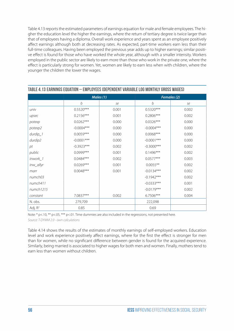
iess Improving effectiveness in social security56
Table 4.13 reports the estimated parameters of earnings equation for male and female employees. The hi-gher the education level the higher the earnings, where the return of tertiary degree is twice larger than that of employees having a diploma. Overall work experience and years spent as an employee positively affect earnings although both at decreasing rates. As expected, part-time workers earn less than their full-time colleagues. Having been employed the previous year adds up to higher earnings; similar positi-ve effect is found for those who have worked the whole year, although with a smaller intensity. Workers employed in the public sector are likely to earn more than those who work in the private one, where the effect is particularly strong for women. Yet, women are likely to earn less when with children, where the younger the children the lower the wages.
Table 4.13 Earnings equation – employees (dependent variable log monthly gross wages)
Males(1) Females(2)
b se b se
univ 0.5520*** 0.001 0.5320*** 0.002
upsec 0.2156*** 0.001 0.2806*** 0.002
potexp 0.0262*** 0.000 0.0326*** 0.000
potexp2 -0.0004*** 0.000 -0.0004*** 0.000
durdip_1 0.0059*** 0.000 0.0068*** 0.000
durdip2 -0.0001*** 0.000 -0.0001*** 0.000
pt -0.3923*** 0.002 -0.3000*** 0.002
public 0.0999*** 0.001 0.1496*** 0.002
inwork_1 0.0484*** 0.002 0.0577*** 0.003
inw_allyr 0.0269*** 0.001 0.0055** 0.002
marr 0.0048*** 0.001 -0.0134*** 0.002
numch03 -0.1942*** 0.002
numch411 -0.0333*** 0.001
numch1215 -0.0179*** 0.002
constant 7.0837*** 0.002 6.7506*** 0.004
N. obs. 279,709 222,098
Adj. R2 0.85 0.69
Note: * p<.10, ** p<.05, *** p<.01. Time dummies are also included in the regressions, not presented here.
Source: T-DYMM 2.0 - own calculations
Table 4.14 shows the results of the estimates of monthly earnings of self-employed workers. Education level and work experience positively affect earnings, where for the first the effect is stronger for men than for women, while no significant difference between gender is found for the acquired experience. Similarly, being married is associated to higher wages for both men and women. Finally, mothers tend to earn less than women without children.
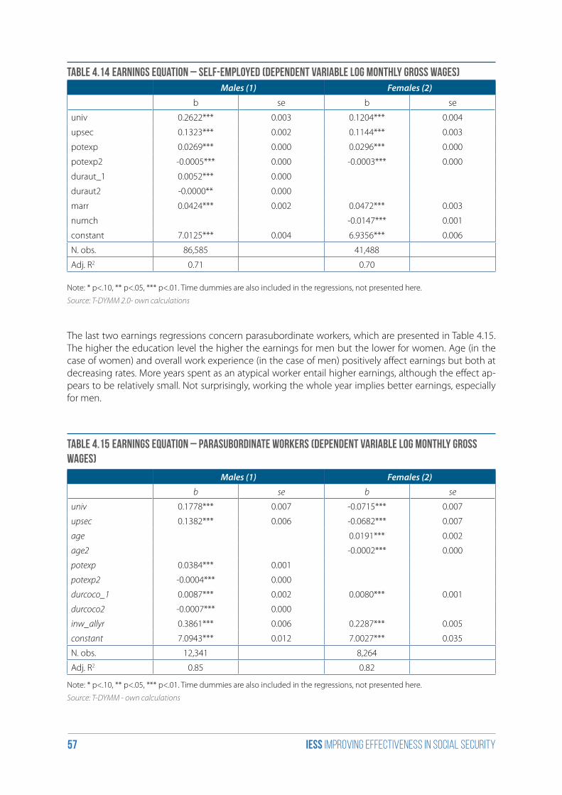
iess Improving effectiveness in social security57
Table 4.14 Earnings equation – self-employed (dependent variable log monthly gross wages)Males(1) Females(2)
b se b se
univ 0.2622*** 0.003 0.1204*** 0.004
upsec 0.1323*** 0.002 0.1144*** 0.003
potexp 0.0269*** 0.000 0.0296*** 0.000
potexp2 -0.0005*** 0.000 -0.0003*** 0.000
duraut_1 0.0052*** 0.000
duraut2 -0.0000** 0.000
marr 0.0424*** 0.002 0.0472*** 0.003
numch -0.0147*** 0.001
constant 7.0125*** 0.004 6.9356*** 0.006
N. obs. 86,585 41,488
Adj. R2 0.71 0.70
Note: * p<.10, ** p<.05, *** p<.01. Time dummies are also included in the regressions, not presented here.
Source: T-DYMM 2.0- own calculations
The last two earnings regressions concern parasubordinate workers, which are presented in Table 4.15. The higher the education level the higher the earnings for men but the lower for women. Age (in the case of women) and overall work experience (in the case of men) positively affect earnings but both at decreasing rates. More years spent as an atypical worker entail higher earnings, although the effect ap-pears to be relatively small. Not surprisingly, working the whole year implies better earnings, especially for men.
Table 4.15 Earnings equation – parasubordinate workers (dependent variable log monthly gross wages)
Males(1) Females(2)
b se b se
univ 0.1778*** 0.007 -0.0715*** 0.007
upsec 0.1382*** 0.006 -0.0682*** 0.007
age 0.0191*** 0.002
age2 -0.0002*** 0.000
potexp 0.0384*** 0.001
potexp2 -0.0004*** 0.000
durcoco_1 0.0087*** 0.002 0.0080*** 0.001
durcoco2 -0.0007*** 0.000
inw_allyr 0.3861*** 0.006 0.2287*** 0.005
constant 7.0943*** 0.012 7.0027*** 0.035
N. obs. 12,341 8,264
Adj. R2 0.85 0.82
Note: * p<.10, ** p<.05, *** p<.01. Time dummies are also included in the regressions, not presented here.
Source: T-DYMM - own calculations
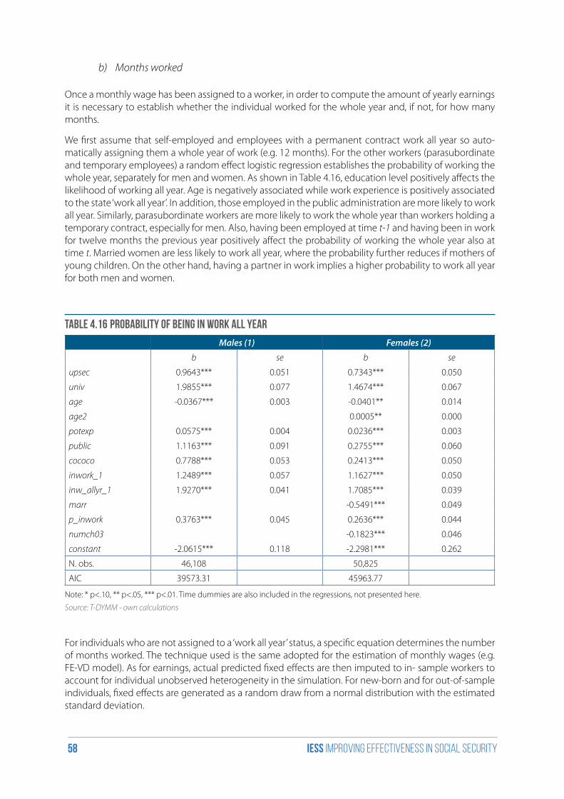
iess Improving effectiveness in social security58
b) Months worked
Once a monthly wage has been assigned to a worker, in order to compute the amount of yearly earnings it is necessary to establish whether the individual worked for the whole year and, if not, for how many months.
We first assume that self-employed and employees with a permanent contract work all year so auto-matically assigning them a whole year of work (e.g. 12 months). For the other workers (parasubordinate and temporary employees) a random effect logistic regression establishes the probability of working the whole year, separately for men and women. As shown in Table 4.16, education level positively affects the likelihood of working all year. Age is negatively associated while work experience is positively associated to the state ‘work all year’. In addition, those employed in the public administration are more likely to work all year. Similarly, parasubordinate workers are more likely to work the whole year than workers holding a temporary contract, especially for men. Also, having been employed at time t-1 and having been in work for twelve months the previous year positively affect the probability of working the whole year also at time t. Married women are less likely to work all year, where the probability further reduces if mothers of young children. On the other hand, having a partner in work implies a higher probability to work all year for both men and women.
Table 4.16 Probability of being in work all year
Males(1) Females(2)
b se b se
upsec 0.9643*** 0.051 0.7343*** 0.050
univ 1.9855*** 0.077 1.4674*** 0.067
age -0.0367*** 0.003 -0.0401** 0.014
age2 0.0005** 0.000
potexp 0.0575*** 0.004 0.0236*** 0.003
public 1.1163*** 0.091 0.2755*** 0.060
cococo 0.7788*** 0.053 0.2413*** 0.050
inwork_1 1.2489*** 0.057 1.1627*** 0.050
inw_allyr_1 1.9270*** 0.041 1.7085*** 0.039
marr -0.5491*** 0.049
p_inwork 0.3763*** 0.045 0.2636*** 0.044
numch03 -0.1823*** 0.046
constant -2.0615*** 0.118 -2.2981*** 0.262
N. obs. 46,108 50,825
AIC 39573.31 45963.77
Note: * p<.10, ** p<.05, *** p<.01. Time dummies are also included in the regressions, not presented here.
Source: T-DYMM - own calculations
For individuals who are not assigned to a ‘work all year’ status, a specific equation determines the number of months worked. The technique used is the same adopted for the estimation of monthly wages (e.g. FE-VD model). As for earnings, actual predicted fixed effects are then imputed to in- sample workers to account for individual unobserved heterogeneity in the simulation. For new-born and for out-of-sample individuals, fixed effects are generated as a random draw from a normal distribution with the estimated standard deviation.
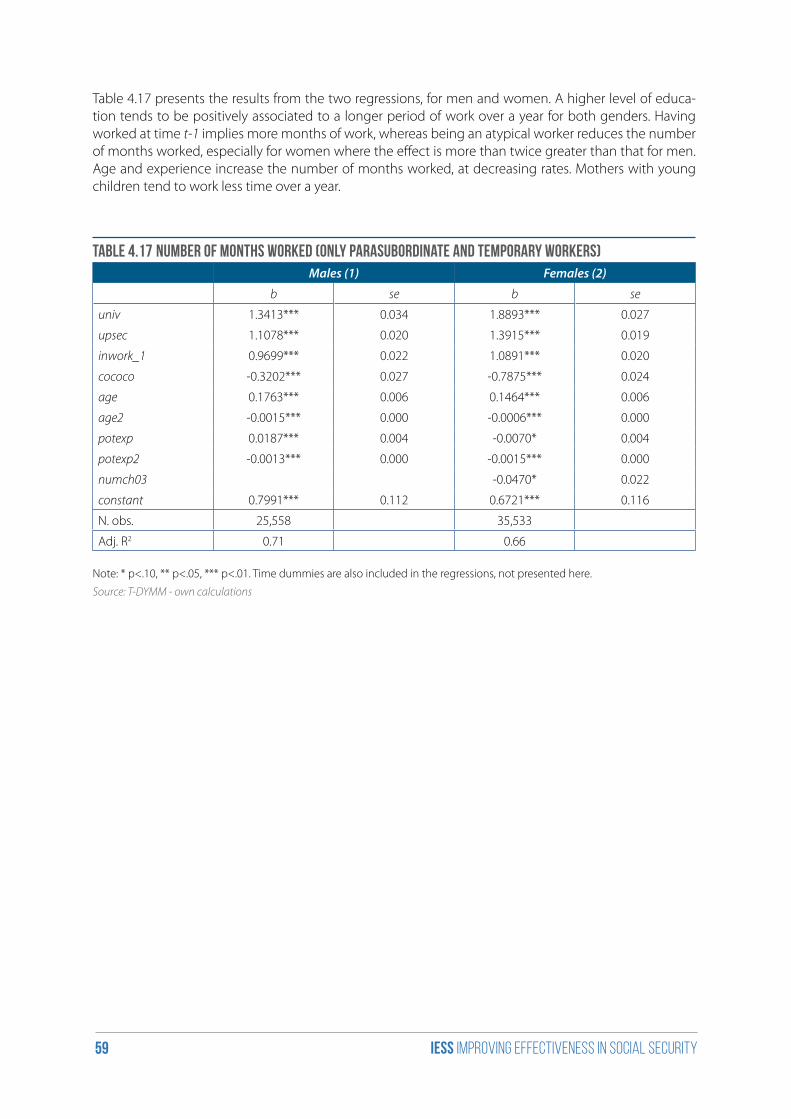
iess Improving effectiveness in social security59
Table 4.17 presents the results from the two regressions, for men and women. A higher level of educa-tion tends to be positively associated to a longer period of work over a year for both genders. Having worked at time t-1 implies more months of work, whereas being an atypical worker reduces the number of months worked, especially for women where the effect is more than twice greater than that for men. Age and experience increase the number of months worked, at decreasing rates. Mothers with young children tend to work less time over a year.
Table 4.17 Number of months worked (only parasubordinate and temporary workers)Males(1) Females(2)
b se b se
univ 1.3413*** 0.034 1.8893*** 0.027
upsec 1.1078*** 0.020 1.3915*** 0.019
inwork_1 0.9699*** 0.022 1.0891*** 0.020
cococo -0.3202*** 0.027 -0.7875*** 0.024
age 0.1763*** 0.006 0.1464*** 0.006
age2 -0.0015*** 0.000 -0.0006*** 0.000
potexp 0.0187*** 0.004 -0.0070* 0.004
potexp2 -0.0013*** 0.000 -0.0015*** 0.000
numch03 -0.0470* 0.022
constant 0.7991*** 0.112 0.6721*** 0.116
N. obs. 25,558 35,533
Adj. R2 0.71 0.66
Note: * p<.10, ** p<.05, *** p<.01. Time dummies are also included in the regressions, not presented here.
Source: T-DYMM - own calculations
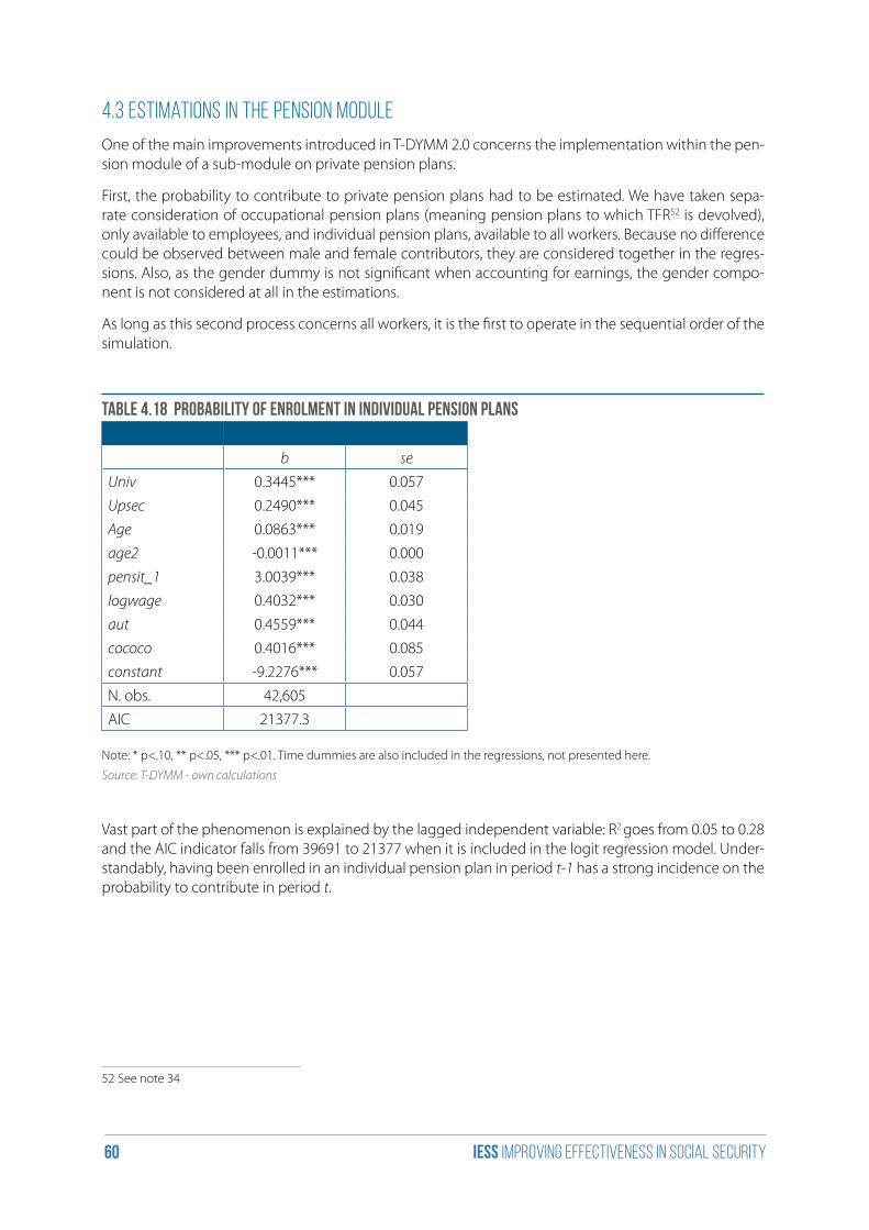
iess Improving effectiveness in social security60
4.3 Estimations in the pension module
One of the main improvements introduced in T-DYMM 2.0 concerns the implementation within the pen-sion module of a sub-module on private pension plans.
First, the probability to contribute to private pension plans had to be estimated. We have taken sepa-rate consideration of occupational pension plans (meaning pension plans to which TFR52 is devolved), only available to employees, and individual pension plans, available to all workers. Because no difference could be observed between male and female contributors, they are considered together in the regres-sions. Also, as the gender dummy is not significant when accounting for earnings, the gender compo-nent is not considered at all in the estimations.
As long as this second process concerns all workers, it is the first to operate in the sequential order of the simulation.
Table 4.18 Probability of enrolment in individual pension plans
b seUniv 0.3445*** 0.057
Upsec 0.2490*** 0.045
Age 0.0863*** 0.019
age2 -0.0011*** 0.000
pensit_1 3.0039*** 0.038
logwage 0.4032*** 0.030
aut 0.4559*** 0.044
cococo 0.4016*** 0.085
constant -9.2276*** 0.057
N. obs. 42,605
AIC 21377.3
Note: * p<.10, ** p<.05, *** p<.01. Time dummies are also included in the regressions, not presented here.
Source: T-DYMM - own calculations
Vast part of the phenomenon is explained by the lagged independent variable: R2 goes from 0.05 to 0.28 and the AIC indicator falls from 39691 to 21377 when it is included in the logit regression model. Under-standably, having been enrolled in an individual pension plan in period t-1 has a strong incidence on the probability to contribute in period t.
52 See note 34
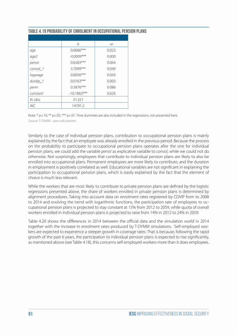
iess Improving effectiveness in social security61
Table 4.19 Probability of enrolment in occupational pension plans
b se
age 0.0666*** 0.023
age2 -0.0009*** 0.000
pensit 0.6583*** 0.064
convol_1 3.7099*** 0.049
logwage 0.6056*** 0.043
durdip_1 0.0163*** 0.003
perm 0.3876*** 0.086
constant -10.1863*** 0.626
N. obs. 31,321
AIC 14791.2
Note: * p<.10, ** p<.05, *** p<.01. Time dummies are also included in the regressions, not presented here.
Source: T-DYMM - own calculations
Similarly to the case of individual pension plans, contribution to occupational pension plans is mainly explained by the fact that an employee was already enrolled in the previous period. Because the process on the probability to participate to occupational pension plans operates after the one for individual pension plans, we could add the variable pensit as explicative variable to convol, while we could not do otherwise. Not surprisingly, employees that contribute to individual pension plans are likely to also be enrolled into occupational plans. Permanent employees are more likely to contribute, and the duration in employment is positively correlated as well. Educational variables are not significant in explaining the participation to occupational pension plans, which is easily explained by the fact that the element of choice is much less relevant.
While the workers that are most likely to contribute to private pension plans are defined by the logistic regressions presented above, the share of workers enrolled in private pension plans is determined by alignment procedures. Taking into account data on enrolment rates registered by COVIP from to 2008 to 2014 and evolving the trend with logarithmic functions, the participation rate of employees to oc-cupational pension plans is projected to stay constant at 15% from 2012 to 2059, while quota of overall workers enrolled in individual pension plans is projected to raise from 14% in 2012 to 24% in 2059.
Table 4.20 shows the differences in 2014 between the official data and the simulation world in 2014 together with the increase in enrolment rates produced by T-DYMM simulations. Self-employed wor-kers are expected to experience a steeper growth in coverage rates. That is because, following the rapid growth of the past 6 years, the participation to individual pension plans is expected to rise significantly, as mentioned above (see Table 4.18), this concerns self-employed workers more than it does employees.
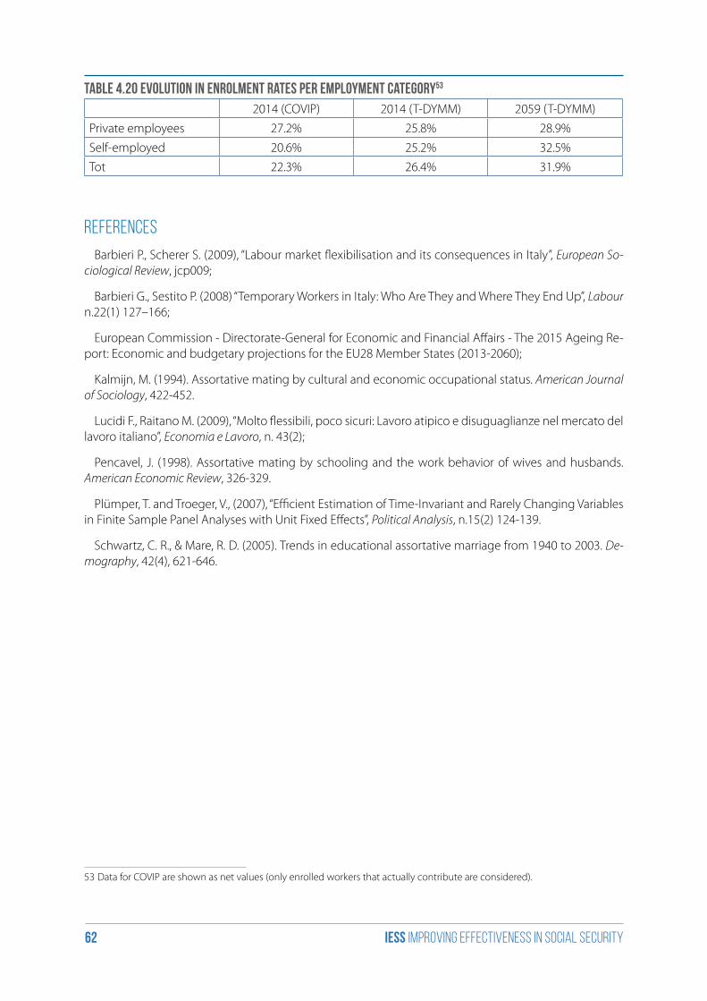
iess Improving effectiveness in social security62
Table 4.20 Evolution in enrolment rates per employment category53
2014 (COVIP) 2014 (T-DYMM) 2059 (T-DYMM)
Private employees 27.2% 25.8% 28.9%
Self-employed 20.6% 25.2% 32.5%
Tot 22.3% 26.4% 31.9%
References
Barbieri P., Scherer S. (2009), “Labour market flexibilisation and its consequences in Italy”, European So-ciological Review, jcp009;
Barbieri G., Sestito P. (2008) “Temporary Workers in Italy: Who Are They and Where They End Up”, Labour n.22(1) 127–166;
European Commission - Directorate-General for Economic and Financial Affairs - The 2015 Ageing Re-port: Economic and budgetary projections for the EU28 Member States (2013-2060);
Kalmijn, M. (1994). Assortative mating by cultural and economic occupational status. American Journal of Sociology, 422-452.
Lucidi F., Raitano M. (2009), “Molto flessibili, poco sicuri: Lavoro atipico e disuguaglianze nel mercato del lavoro italiano”, Economia e Lavoro, n. 43(2);
Pencavel, J. (1998). Assortative mating by schooling and the work behavior of wives and husbands. American Economic Review, 326-329.
Plümper, T. and Troeger, V., (2007), “Efficient Estimation of Time-Invariant and Rarely Changing Variables in Finite Sample Panel Analyses with Unit Fixed Effects”, Political Analysis, n.15(2) 124-139.
Schwartz, C. R., & Mare, R. D. (2005). Trends in educational assortative marriage from 1940 to 2003. De-mography, 42(4), 621-646.
53 Data for COVIP are shown as net values (only enrolled workers that actually contribute are considered).

iess Improving effectiveness in social security63
5. Simulation results
Before analysing the main outcomes of T-DYMM 2.0’s simulations in their present state, it is of some importance to sum up the key assumptions underlying the results and have a look at the impact on the evolution of the pension system.
three typologies of assumptions may be identified: demographic, macroeconomic and microeconomic assumptions.
a. Demographic assumptions on fertility rate, migration and life expectancy.
Assumptions on fertility rate and migration54 have an impact on sustainability indicators, which are not shown here. Changes in life expectancy affect eligibility requirements as well as the computation of pen-sion benefits, through the mechanism of automatic adjustment55 of age requirements and conversion coefficients56 to changes in longevity.
b. Macroeconomic assumptions on GDP growth, employment rate, inflation rate.
In T-DYMM, GDP growth affects the level of wages and the notional revenues on contributions paid in the NDC system. Because of the intrinsic characteristics of NDC pension systems, workers’ condition is affected by employment rates not only during activity, but also during retirement, since possible unem-ployment spells have an impact on the accruement of notional contributions and the eventual level of pension benefits.
Since pension benefits in Italy are indexed to inflation according to given thresholds, assumptions on inflation rates define how much and how fast pensions lose purchasing power compared to wages.
c. Microeconomic assumptions on career patterns and retirement choices.
Again, because of the mirroring proprieties of NDC pension schemes, stability and dynamics of working careers, whose patterns are estimated on AD-SILC, impact on workers’ income conditions before and after retirement. Following principles of actuarial fairness, the age in which individuals choose to retire is directly related to the amount of benefit they will receive.
As far as retirement choices are concerned, results shown in the present chapter pertain to two scenarios:
1. “No-choice scenario”, where we assume that individuals retire as soon as they reach retirement re-quisites;
2. “Choice scenario”, where we assume that, if workers fulfil the criteria for early retirement but have not reached the statutory age requirements for old-age retirement, they will leave the labour market only if their potential replacement rate exceeds 60%57.
54 As of today, T-DYMM 2.0 – like its predecessor – is a “closed” model, assuming “zero migration”.55 Introduced by Law n. 122/2010 – partially modified by the more recent 2011 pension reform56 The conversion coefficient, sometimes referred to as “divisor”, is the operator that converts the amount of (notional) capital accrued into an annuity.57 60% is the Gross Average Replacement Rate registered in Italy in 2013 (AWG, 2015).
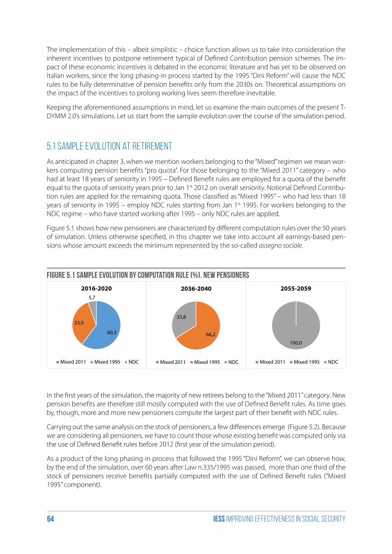
iess Improving effectiveness in social security64
The implementation of this – albeit simplistic – choice function allows us to take into consideration the inherent incentives to postpone retirement typical of Defined Contribution pension schemes. The im-pact of these economic incentives is debated in the economic literature and has yet to be observed on Italian workers, since the long phasing-in process started by the 1995 “Dini Reform” will cause the NDC rules to be fully determinative of pension benefits only from the 2030s on. Theoretical assumptions on the impact of the incentives to prolong working lives seem therefore inevitable.
Keeping the aforementioned assumptions in mind, let us examine the main outcomes of the present T-DYMM 2.0’s simulations. Let us start from the sample evolution over the course of the simulation period.
5.1 Sample evolution at retirement
As anticipated in chapter 3, when we mention workers belonging to the “Mixed” regimen we mean wor-kers computing pension benefits “pro quota”. For those belonging to the “Mixed 2011” category – who had at least 18 years of seniority in 1995 – Defined Benefit rules are employed for a quota of the benefit equal to the quota of seniority years prior to Jan 1st 2012 on overall seniority. Notional Defined Contribu-tion rules are applied for the remaining quota. Those classified as “Mixed 1995” – who had less than 18 years of seniority in 1995 – employ NDC rules starting from Jan 1st 1995. For workers belonging to the NDC regime – who have started working after 1995 – only NDC rules are applied.
Figure 5.1 shows how new pensioners are characterized by different computation rules over the 50 years of simulation. Unless otherwise specified, in this chapter we take into account all earnings-based pen-sions whose amount exceeds the minimum represented by the so-called assegno sociale.
Figure 5.1 Sample evolution by computation rule (%). New pensioners
60,3
33,9
5,7
2016-2020
Mixed 2011 Mixed 1995 NDC
66,2
33,8
2036-2040
Mixed 2011 Mixed 1995 NDC
100,0
2055-2059
Mixed 2011 Mixed 1995 NDC
In the first years of the simulation, the majority of new retirees belong to the “Mixed 2011” category. New pension benefits are therefore still mostly computed with the use of Defined Benefit rules. As time goes by, though, more and more new pensioners compute the largest part of their benefit with NDC rules.
Carrying out the same analysis on the stock of pensioners, a few differences emerge (Figure 5.2). Because we are considering all pensioners, we have to count those whose existing benefit was computed only via the use of Defined Benefit rules before 2012 (first year of the simulation period).
As a product of the long phasing-in process that followed the 1995 “Dini Reform”, we can observe how, by the end of the simulation, over 60 years after Law n.335/1995 was passed, more than one third of the stock of pensioners receive benefits partially computed with the use of Defined Benefit rules (“Mixed 1995” component).
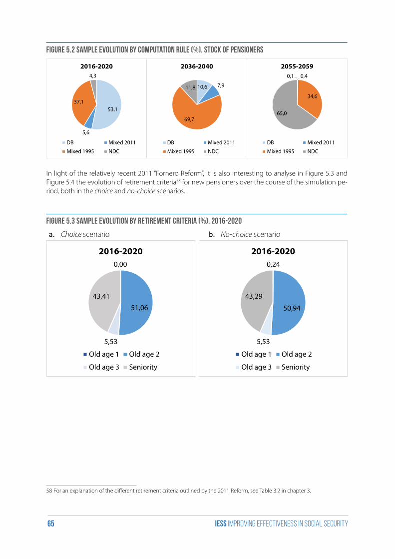
iess Improving effectiveness in social security65
Figure 5.2 Sample evolution by computation rule (%). Stock of pensioners
53,1
5,6
37,1
4,3
2016-2020
DB Mixed 2011
Mixed 1995 NDC
10,6 7,9
69,7
11,8
2036-2040
DB Mixed 2011
Mixed 1995 NDC
0,1 0,4
34,6
65,0
2055-2059
DB Mixed 2011
Mixed 1995 NDC
In light of the relatively recent 2011 “Fornero Reform”, it is also interesting to analyse in Figure 5.3 and Figure 5.4 the evolution of retirement criteria58 for new pensioners over the course of the simulation pe-riod, both in the choice and no-choice scenarios.
Figure 5.3 Sample evolution by retirement criteria (%). 2016-2020
a. Choice scenario b. No-choice scenario
0,00
51,06
5,53
43,41
2016-2020
Old age 1 Old age 2
Old age 3 Seniority
0,24
50,94
5,53
43,29
2016-2020
Old age 1 Old age 2
Old age 3 Seniority
58 For an explanation of the different retirement criteria outlined by the 2011 Reform, see Table 3.2 in chapter 3.
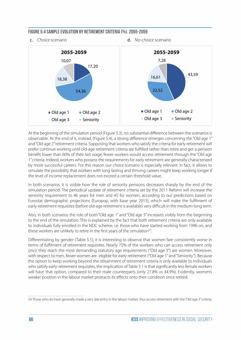
iess Improving effectiveness in social security66
Figure 5.4 Sample evolution by retirement criteria (%). 2055-2059
c. Choice scenario d. No-choice scenario
17,20
54,36
18,38
10,07
2055-2059
Old age 1 Old age 2
Old age 3 Seniority
43,59
32,52
16,61
7,28
2055-2059
Old age 1 Old age 2
Old age 3 Seniority
At the beginning of the simulation period (Figure 5.3), no substantial difference between the scenarios is observable. At the end of it, instead, (Figure 5.4), a strong difference emerges concerning the “Old age 1” and “Old age 2” retirement criteria. Supposing that workers who satisfy the criteria for early retirement will prefer continue working until old-age retirement criteria are fulfilled rather than retire and get a pension benefit lower than 60% of their last wage, fewer workers would access retirement through the “Old age 1” criteria. Indeed, workers who possess the requirements for early retirement are generally characterized by more successful careers. For this reason our choice scenario is especially relevant: in fact, it allows to simulate the possibility that workers with long-lasting and thriving careers might keep working longer if the level of income replacement does not exceed a certain threshold value.
In both scenarios, it is visible how the role of seniority pensions decreases sharply by the end of the simulation period. The periodical update of retirement criteria set by the 2011 Reform will increase the seniority requirement to 46 years for men and 45 for women, according to our predictions based on Eurostat demographic projections (Europop, with base year 2013), which will make the fulfilment of early-retirement requisites (before old-age retirement is available) very difficult in the medium-long term.
Also, in both scenarios the role of both “Old age 1” and “Old age 3” increases visibly from the beginning to the end of the simulation. This is explained by the fact that both retirement criteria are only available to individuals fully enrolled in the NDC scheme, i.e. those who have started working from 1996 on, and these workers are unlikely to retire in the first years of the simulation59.
Differentiating by gender (Table 5.1), it is interesting to observe that women fare consistently worse in terms of fulfilment of retirement requisites. Nearly 75% of the workers who can access retirement only once they reach the most demanding statutory age requirements (“Old age 3”) are women. Moreover, with respect to men, fewer women are eligible for early retirement (“Old age 1” and “Seniority”). Because the option to keep working beyond the obtainment of retirement criteria is only available to individuals who satisfy early-retirement requisites, the implication of Table 5.1 is that significantly less female workers will have that option, compared to their male counterparts (only 27.8% vs 44.9%). Evidently, women’s weaker position in the labour market protracts its effects onto their condition once retired.
59 Those who do have generally made a very late entry in the labour market, thus access retirement with the “Old age 3” criteria.
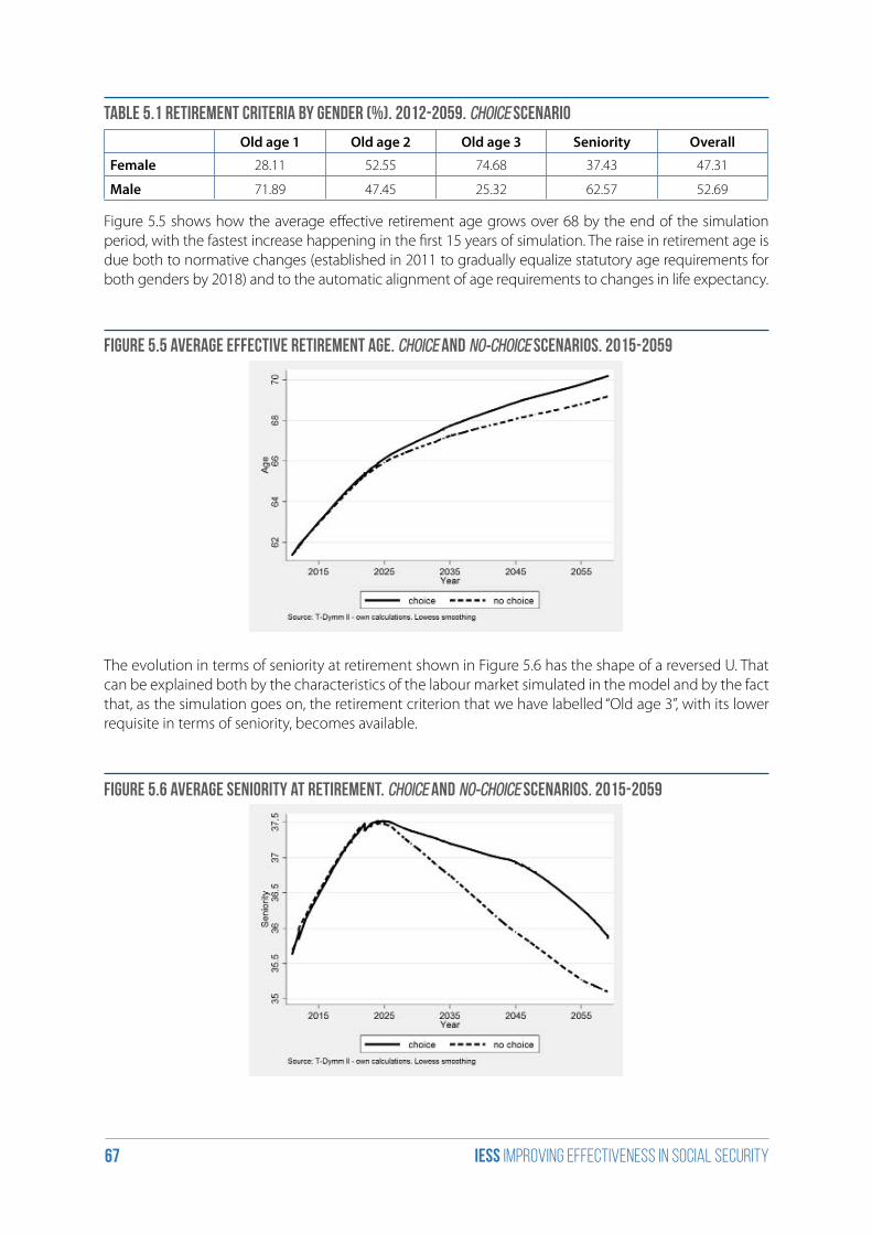
iess Improving effectiveness in social security67
Table 5.1 Retirement criteria by gender (%). 2012-2059. ChoiCe scenario
Old age 1 Old age 2 Old age 3 Seniority Overall
Female 28.11 52.55 74.68 37.43 47.31
Male 71.89 47.45 25.32 62.57 52.69
Figure 5.5 shows how the average effective retirement age grows over 68 by the end of the simulation period, with the fastest increase happening in the first 15 years of simulation. The raise in retirement age is due both to normative changes (established in 2011 to gradually equalize statutory age requirements for both genders by 2018) and to the automatic alignment of age requirements to changes in life expectancy.
Figure 5.5 Average effective retirement age. ChoiCe and no-ChoiCe scenarios. 2015-2059
The evolution in terms of seniority at retirement shown in Figure 5.6 has the shape of a reversed U. That can be explained both by the characteristics of the labour market simulated in the model and by the fact that, as the simulation goes on, the retirement criterion that we have labelled “Old age 3”, with its lower requisite in terms of seniority, becomes available.
Figure 5.6 Average seniority at retirement. ChoiCe and no-ChoiCe scenarios. 2015-2059
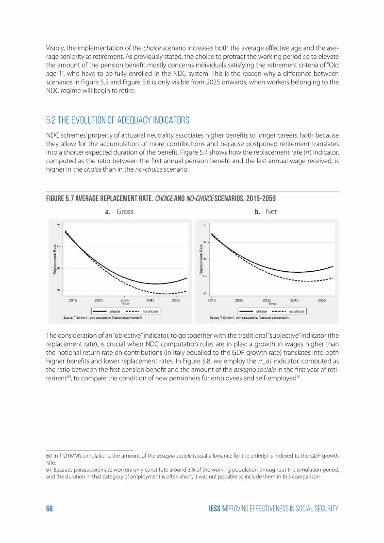
iess Improving effectiveness in social security68
Visibly, the implementation of the choice scenario increases both the average effective age and the ave-rage seniority at retirement. As previously stated, the choice to protract the working period so to elevate the amount of the pension benefit mostly concerns individuals satisfying the retirement criteria of “Old age 1”, who have to be fully enrolled in the NDC system. This is the reason why a difference between scenarios in Figure 5.5 and Figure 5.6 is only visible from 2025 onwards, when workers belonging to the NDC regime will begin to retire.
5.2 The evolution of adequacy indicators
NDC schemes’ property of actuarial neutrality associates higher benefits to longer careers, both because they allow for the accumulation of more contributions and because postponed retirement translates into a shorter expected duration of the benefit. Figure 5.7 shows how the replacement rate (rr) indicator, computed as the ratio between the first annual pension benefit and the last annual wage received, is higher in the choice than in the no-choice scenario.
Figure 5.7 Average replacement rate. ChoiCe and no-ChoiCe scenarios. 2015-2059
a. Gross b. Net
The consideration of an “objective” indicator, to go together with the traditional “subjective” indicator (the replacement rate), is crucial when NDC computation rules are in play: a growth in wages higher than the notional return rate on contributions (in Italy equalled to the GDP growth rate) translates into both higher benefits and lower replacement rates. In Figure 5.8, we employ the rr_as indicator, computed as the ratio between the first pension benefit and the amount of the assegno sociale in the first year of reti-rement60, to compare the condition of new pensioners for employees and self-employed61.
60 In T-DYMM’s simulations, the amount of the assegno sociale (social allowance for the elderly) is indexed to the GDP growth rate.61 Because parasubordinate workers only constitute around 3% of the working population throughout the simulation period, and the duration in that category of employment is often short, it was not possible to include them in this comparison.
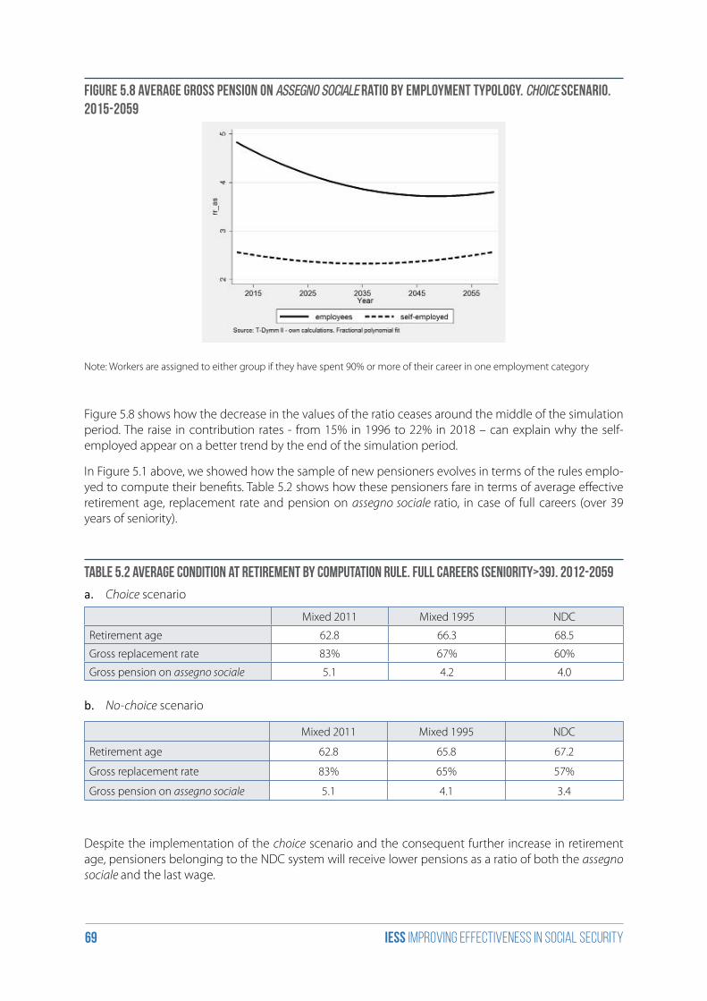
iess Improving effectiveness in social security69
Figure 5.8 Average gross pension on assegno soCiale ratio by employment typology. ChoiCe scenario. 2015-2059
Note: Workers are assigned to either group if they have spent 90% or more of their career in one employment category
Figure 5.8 shows how the decrease in the values of the ratio ceases around the middle of the simulation period. The raise in contribution rates - from 15% in 1996 to 22% in 2018 – can explain why the self-employed appear on a better trend by the end of the simulation period.
In Figure 5.1 above, we showed how the sample of new pensioners evolves in terms of the rules emplo-yed to compute their benefits. Table 5.2 shows how these pensioners fare in terms of average effective retirement age, replacement rate and pension on assegno sociale ratio, in case of full careers (over 39 years of seniority).
Table 5.2 Average condition at retirement by computation rule. Full careers (seniority>39). 2012-2059
a. Choice scenario
Mixed 2011 Mixed 1995 NDC
Retirement age 62.8 66.3 68.5
Gross replacement rate 83% 67% 60%
Gross pension on assegno sociale 5.1 4.2 4.0
b. No-choice scenario
Mixed 2011 Mixed 1995 NDC
Retirement age 62.8 65.8 67.2
Gross replacement rate 83% 65% 57%
Gross pension on assegno sociale 5.1 4.1 3.4
Despite the implementation of the choice scenario and the consequent further increase in retirement age, pensioners belonging to the NDC system will receive lower pensions as a ratio of both the assegno sociale and the last wage.
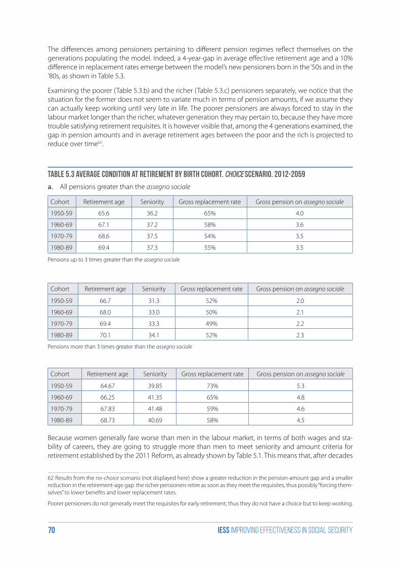
iess Improving effectiveness in social security70
The differences among pensioners pertaining to different pension regimes reflect themselves on the generations populating the model. Indeed, a 4-year-gap in average effective retirement age and a 10% difference in replacement rates emerge between the model’s new pensioners born in the ‘50s and in the ‘80s, as shown in Table 5.3.
Examining the poorer (Table 5.3.b) and the richer (Table 5.3.c) pensioners separately, we notice that the situation for the former does not seem to variate much in terms of pension amounts, if we assume they can actually keep working until very late in life. The poorer pensioners are always forced to stay in the labour market longer than the richer, whatever generation they may pertain to, because they have more trouble satisfying retirement requisites. It is however visible that, among the 4 generations examined, the gap in pension amounts and in average retirement ages between the poor and the rich is projected to reduce over time62.
Table 5.3 Average condition at retirement by birth cohort. ChoiCe scenario. 2012-2059
a. All pensions greater than the assegno sociale
Cohort Retirement age Seniority Gross replacement rate Gross pension on assegno sociale
1950-59 65.6 36.2 65% 4.0
1960-69 67.1 37.2 58% 3.6
1970-79 68.6 37.5 54% 3.5
1980-89 69.4 37.3 55% 3.5
Pensions up to 3 times greater than the assegno sociale
Cohort Retirement age Seniority Gross replacement rate Gross pension on assegno sociale
1950-59 66.7 31.3 52% 2.0
1960-69 68.0 33.0 50% 2.1
1970-79 69.4 33.3 49% 2.2
1980-89 70.1 34.1 52% 2.3
Pensions more than 3 times greater than the assegno sociale
Cohort Retirement age Seniority Gross replacement rate Gross pension on assegno sociale
1950-59 64.67 39.85 73% 5.3
1960-69 66.25 41.35 65% 4.8
1970-79 67.83 41.48 59% 4.6
1980-89 68.73 40.69 58% 4.5
Because women generally fare worse than men in the labour market, in terms of both wages and sta-bility of careers, they are going to struggle more than men to meet seniority and amount criteria for retirement established by the 2011 Reform, as already shown by Table 5.1. This means that, after decades
62 Results from the no-choice scenario (not displayed here) show a greater reduction in the pension-amount gap and a smaller reduction in the retirement-age gap: the richer pensioners retire as soon as they meet the requisites, thus possibly “forcing them-selves” to lower benefits and lower replacement rates.
Poorer pensioners do not generally meet the requisites for early retirement, thus they do not have a choice but to keep working.
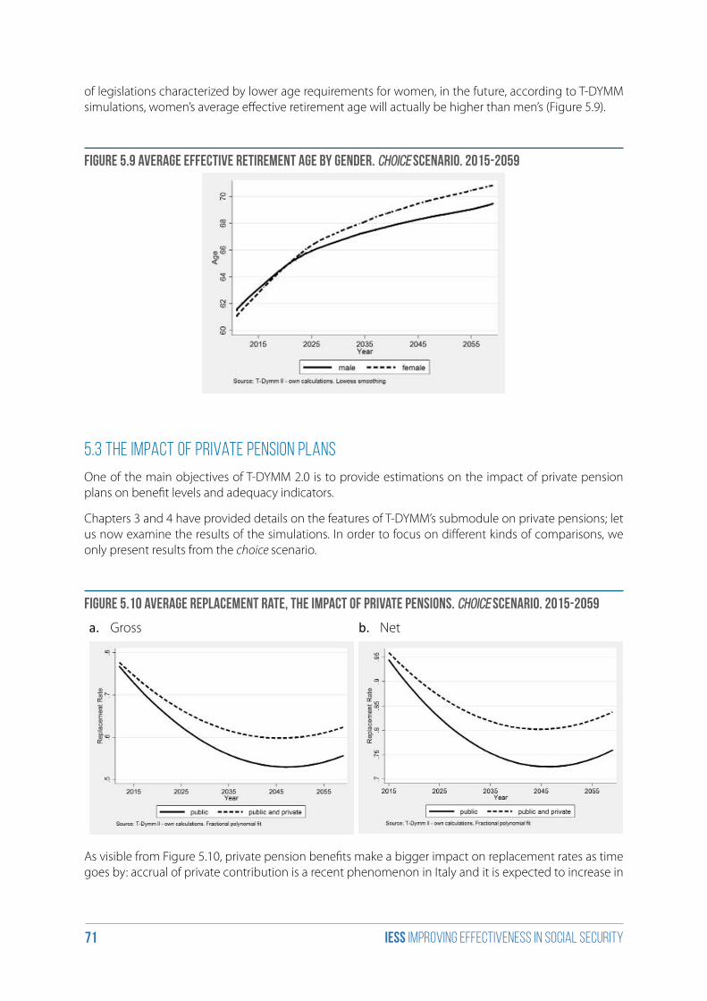
iess Improving effectiveness in social security71
of legislations characterized by lower age requirements for women, in the future, according to T-DYMM simulations, women’s average effective retirement age will actually be higher than men’s (Figure 5.9).
Figure 5.9 Average effective retirement age by gender. ChoiCe scenario. 2015-2059
5.3 The impact of private pension plans
One of the main objectives of T-DYMM 2.0 is to provide estimations on the impact of private pension plans on benefit levels and adequacy indicators.
Chapters 3 and 4 have provided details on the features of T-DYMM’s submodule on private pensions; let us now examine the results of the simulations. In order to focus on different kinds of comparisons, we only present results from the choice scenario.
Figure 5.10 Average replacement rate, the impact of private pensions. ChoiCe scenario. 2015-2059
a. Gross b. Net
As visible from Figure 5.10, private pension benefits make a bigger impact on replacement rates as time goes by: accrual of private contribution is a recent phenomenon in Italy and it is expected to increase in
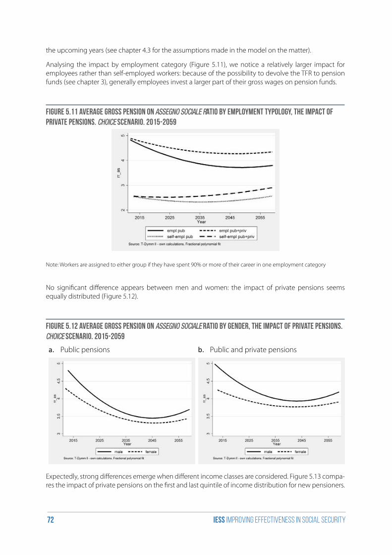
iess Improving effectiveness in social security72
the upcoming years (see chapter 4.3 for the assumptions made in the model on the matter).
Analysing the impact by employment category (Figure 5.11), we notice a relatively larger impact for employees rather than self-employed workers: because of the possibility to devolve the TFR to pension funds (see chapter 3), generally employees invest a larger part of their gross wages on pension funds.
Figure 5.11 Average gross pension on assegno soCiale ratio by employment typology, the impact of private pensions. ChoiCe scenario. 2015-2059
Note: Workers are assigned to either group if they have spent 90% or more of their career in one employment category
No significant difference appears between men and women: the impact of private pensions seems equally distributed (Figure 5.12).
Figure 5.12 Average gross pension on assegno soCiale ratio by gender, the impact of private pensions. ChoiCe scenario. 2015-2059
a. Public pensions b. Public and private pensions
Expectedly, strong differences emerge when different income classes are considered. Figure 5.13 compa-res the impact of private pensions on the first and last quintile of income distribution for new pensioners.
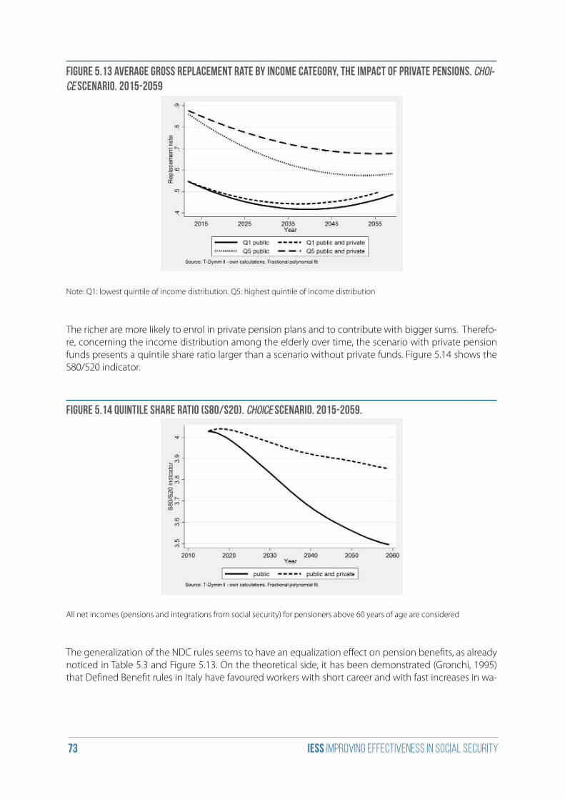
iess Improving effectiveness in social security73
Figure 5.13 Average gross replacement rate by income category, the impact of private pensions. Choi-Ce scenario. 2015-2059
Note: Q1: lowest quintile of income distribution. Q5: highest quintile of income distribution
The richer are more likely to enrol in private pension plans and to contribute with bigger sums. Therefo-re, concerning the income distribution among the elderly over time, the scenario with private pension funds presents a quintile share ratio larger than a scenario without private funds. Figure 5.14 shows the S80/S20 indicator.
Figure 5.14 Quintile share ratio (S80/S20). ChoiCe scenario. 2015-2059.
All net incomes (pensions and integrations from social security) for pensioners above 60 years of age are considered
The generalization of the NDC rules seems to have an equalization effect on pension benefits, as already noticed in Table 5.3 and Figure 5.13. On the theoretical side, it has been demonstrated (Gronchi, 1995) that Defined Benefit rules in Italy have favoured workers with short career and with fast increases in wa-
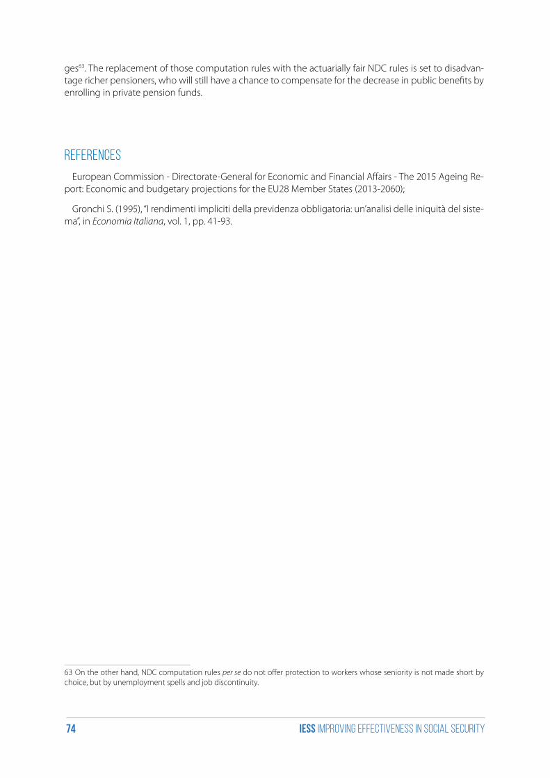
iess Improving effectiveness in social security74
ges63. The replacement of those computation rules with the actuarially fair NDC rules is set to disadvan-tage richer pensioners, who will still have a chance to compensate for the decrease in public benefits by enrolling in private pension funds.
References
European Commission - Directorate-General for Economic and Financial Affairs - The 2015 Ageing Re-port: Economic and budgetary projections for the EU28 Member States (2013-2060);
Gronchi S. (1995), “I rendimenti impliciti della previdenza obbligatoria: un’analisi delle iniquità del siste-ma”, in Economia Italiana, vol. 1, pp. 41-93.
63 On the other hand, NDC computation rules per se do not offer protection to workers whose seniority is not made short by choice, but by unemployment spells and job discontinuity.
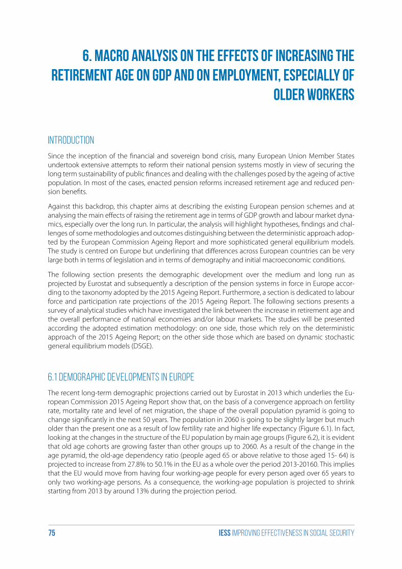
iess Improving effectiveness in social security75
6. Macro analysis on the effects of increasing the retirement age on GDP and on employment, especially of
older workers
Introduction
Since the inception of the financial and sovereign bond crisis, many European Union Member States undertook extensive attempts to reform their national pension systems mostly in view of securing the long term sustainability of public finances and dealing with the challenges posed by the ageing of active population. In most of the cases, enacted pension reforms increased retirement age and reduced pen-sion benefits.
Against this backdrop, this chapter aims at describing the existing European pension schemes and at analysing the main effects of raising the retirement age in terms of GDP growth and labour market dyna-mics, especially over the long run. In particular, the analysis will highlight hypotheses, findings and chal-lenges of some methodologies and outcomes distinguishing between the deterministic approach adop-ted by the European Commission Ageing Report and more sophisticated general equilibrium models. The study is centred on Europe but underlining that differences across European countries can be very large both in terms of legislation and in terms of demography and initial macroeconomic conditions.
The following section presents the demographic development over the medium and long run as projected by Eurostat and subsequently a description of the pension systems in force in Europe accor-ding to the taxonomy adopted by the 2015 Ageing Report. Furthermore, a section is dedicated to labour force and participation rate projections of the 2015 Ageing Report. The following sections presents a survey of analytical studies which have investigated the link between the increase in retirement age and the overall performance of national economies and/or labour markets. The studies will be presented according the adopted estimation methodology: on one side, those which rely on the deterministic approach of the 2015 Ageing Report; on the other side those which are based on dynamic stochastic general equilibrium models (DSGE).
6.1 Demographic developments in Europe
The recent long-term demographic projections carried out by Eurostat in 2013 which underlies the Eu-ropean Commission 2015 Ageing Report show that, on the basis of a convergence approach on fertility rate, mortality rate and level of net migration, the shape of the overall population pyramid is going to change significantly in the next 50 years. The population in 2060 is going to be slightly larger but much older than the present one as a result of low fertility rate and higher life expectancy (Figure 6.1). In fact, looking at the changes in the structure of the EU population by main age groups (Figure 6.2), it is evident that old age cohorts are growing faster than other groups up to 2060. As a result of the change in the age pyramid, the old-age dependency ratio (people aged 65 or above relative to those aged 15- 64) is projected to increase from 27.8% to 50.1% in the EU as a whole over the period 2013-20160. This implies that the EU would move from having four working-age people for every person aged over 65 years to only two working-age persons. As a consequence, the working-age population is projected to shrink starting from 2013 by around 13% during the projection period.
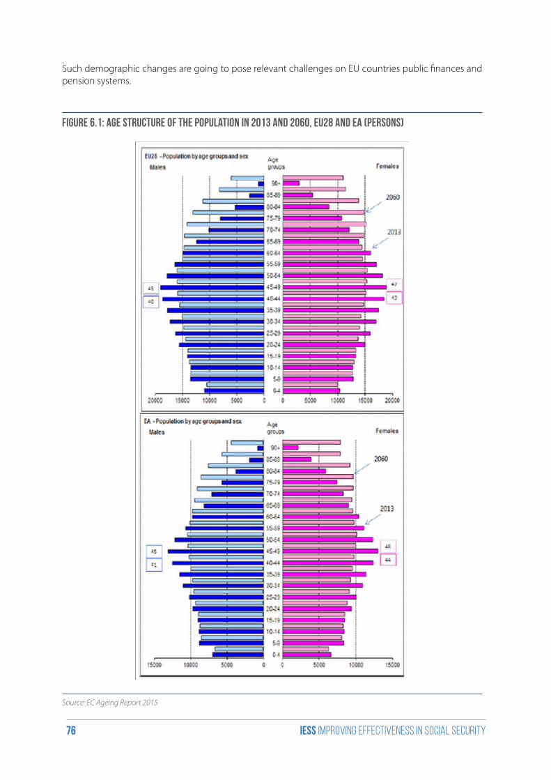
iess Improving effectiveness in social security76
Such demographic changes are going to pose relevant challenges on EU countries public finances and pension systems.
Figure 6.1: Age structure of the population in 2013 and 2060, EU28 and EA (persons)
Source: EC Ageing Report 2015
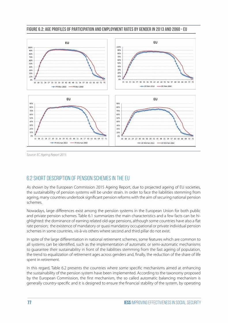
iess Improving effectiveness in social security77
Figure 6.2: Age profiles of participation and employment rates by gender in 2013 and 2060 - EU
Source: EC Ageing Report 2015
6.2 Short description of pension schemes in the EU
As shown by the European Commission 2015 Ageing Report, due to projected ageing of EU societies, the sustainability of pension systems will be under strain. In order to face the liabilities stemming from ageing, many countries undertook significant pension reforms with the aim of securing national pension schemes.
Nowadays, large differences exist among the pension systems in the European Union for both public and private pension schemes. Table 6.1 summarizes the main characteristics and a few facts can be hi-ghlighted: the dominance of earning related old-age pensions, although some countries have also a flat rate pension; the existence of mandatory or quasi mandatory occupational or private individual pension schemes in some countries, vis-à-vis others where second and third pillar do not exist.
In spite of the large differentiation in national retirement schemes, some features which are common to all systems can be identified, such as the implementation of automatic or semi-automatic mechanisms to guarantee their sustainability in front of the liabilities stemming from the fast ageing of population, the trend to equalization of retirement ages across genders and, finally, the reduction of the share of life spent in retirement.
In this regard, Table 6.2 presents the countries where some specific mechanisms aimed at enhancing the sustainability of the pension system have been implemented. According to the taxonomy proposed by the European Commission, the first mechanism, the so called automatic balancing mechanism is generally country-specific and it is designed to ensure the financial stability of the system, by operating
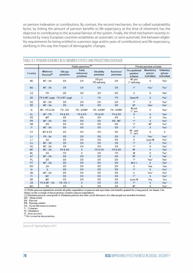
iess Improving effectiveness in social security78
on pension indexation or contributions. By contrast, the second mechanism, the so called sustainability factor, by linking the amount of pension benefits to life expectancy at the time of retirement has the objective to contributing to the actuarial fairness of the system. Finally, the third mechanism recently in-troduced by many European countries establishes an automatic or semi-automatic link between eligibi-lity requirements for being entitled to a pension (age and/or years of contributions) and life expectancy, sterilizing in this way the impact of demographic changes.
Table 6.1: Pension schemes in EU Member States and projection coverage
Source: EC Ageing Report 2015
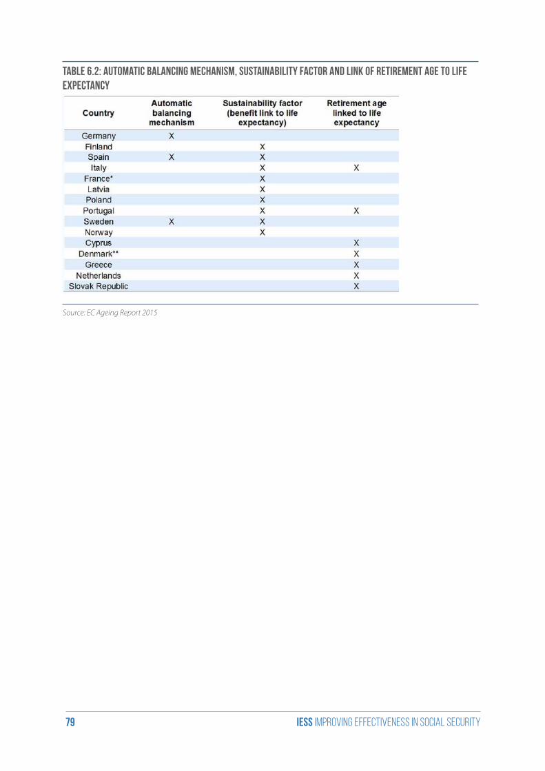
iess Improving effectiveness in social security79
Table 6.2: Automatic balancing mechanism, sustainability factor and link of retirement age to life expectancy
Source: EC Ageing Report 2015
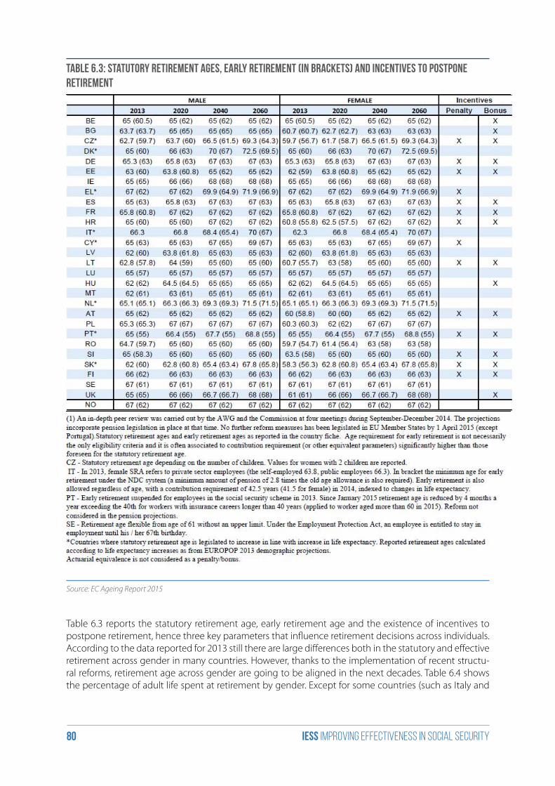
iess Improving effectiveness in social security80
Table 6.3: Statutory retirement ages, early retirement (in brackets) and incentives to postpone retirement
Source: EC Ageing Report 2015
Table 6.3 reports the statutory retirement age, early retirement age and the existence of incentives to postpone retirement, hence three key parameters that influence retirement decisions across individuals. According to the data reported for 2013 still there are large differences both in the statutory and effective retirement across gender in many countries. However, thanks to the implementation of recent structu-ral reforms, retirement age across gender are going to be aligned in the next decades. Table 6.4 shows the percentage of adult life spent at retirement by gender. Except for some countries (such as Italy and
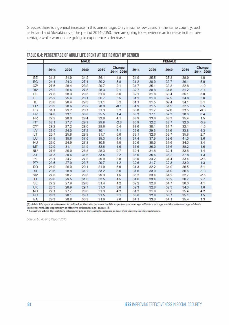
iess Improving effectiveness in social security81
Greece), there is a general increase in this percentage. Only in some few cases, in the same country, such as Poland and Slovakia, over the period 2014-2060, men are going to experience an increase in their per-centage while women are going to experience a decrease.
Table 6.4: Percentage of adult life spent at retirement by gender
Source: EC Ageing Report 2015
iess Improving effectiveness in social security82
6.3 Labour force projections and participation rate: the deterministic approach of the 2015 Ageing Report
According to the European Commission, the increasing ageing of population coupled with the enacted rise in the effective retirement age will have an impact also on labour supply and participation to the labour force in Europe. The European Commission in the 2015 Ageing Report projects participation rates by gender and single age according to the so-called Cohort Simulation Model. Such a method is ba-sed on the calculation of the average probabilities of entry and exit for labour force over the historical period 2004-2013. These probabilities are then extrapolated in the future according to the change in age cohorts as projected by the Eurostat demographic long term scenario. Such a method produces estimates of average exit age from labour force under a no-policy change assumption, i.e. in the absence of implemented pension reforms. However, the Cohort Simulation method is flexible enough to allow to design suitable policy-scenarios in which it is possible to take into account the labour market effect of enacted pension reforms. The main characteristics of pension reforms are applied by single cohort by modifying and increasing average exit rates for different age groups and gender according to the main features of national pension systems. The re-estimation of average exit age from the labour force for single cohorts and for different gender has a non-trivial increasing impact on participation rates and, in turn, on GPD projections.
Based on the age group 50-70, the change in average exit rates by gender due to the impact of pension reforms in 2060, as projected in the 2015 Ageing Report, are reported in Figure 6.3. On average, enacted pension reforms will increase the effective retirement age by almost 5 years in 2060 exerting a large im-pact on labour force participation of older cohorts.
Such a pattern is even more evident in Figure 6.4 which reports the change in participation rates at three points in time: 2020, 2040 and 2060 for different age cohorts. The comparison is made with a scenario where pension reforms had not been implemented. Thanks to pension reforms, the participation rate of older workers (55-74) in the EU is projected to increase by 4 p.p. in 2020, 10 p.p. in 2040 and 11 p.p. in 2060. Overall, the higher participation rate of older workers induced by the postponement of retirement age due to the implementation of pension reforms will have an increasing impact of about 3,5 p.p. by 2060 on the total participation rate (15-74) in EU.
iess Improving effectiveness in social security83
Figure 6.3: Impact of pension reforms on the average effective retirement age from the labour force
Source: EC Ageing Report 2015
iess Improving effectiveness in social security84
Figure 6.4: Projected impact of pension reforms on participation rates (2020, 2040, 2060) in percenta-ge points - comparison of projections with and without pension reforms
Source: EC Ageing Report 2015

iess Improving effectiveness in social security85
6.4 Pension reforms and participation rate: deterministic projections
In order to preserve growth, spur labour participation rates and deal with public finance liabilities linked to ageing, a paper by Schwan and Sail (2013) based on the European Commission deterministic me-thodology has suggested guidelines and recommendations for reforming pension systems. According to this study, two ways to reform pension systems may help to improve fiscal sustainability: eligibility-restricting reforms and generosity-reducing reforms. Even though the two categories are strictly interlin-ked, it is also true that each policy mix can have different impact on labour market participation.
Pension reforms aiming at restricting eligibility requirements normally reduce the coverage rate of pen-sion systems, that is the number of pensioner as a share of population aged above 65. Usually, such a kind of reform has the objective of abolishing or restricting early retirement schemes, increasing statu-tory retirement ages or harmonizing retirement ages between men and women. When analysing the eligibility of a pension system, two specific indicators are investigated: coverage ratios and effective exit age projections, and the gap between effective labour market exit age and statutory retirement age. In almost all countries, average effective ages of exit from labour market are lower than the respective statutory retirement ages. Such an issue could be addressed by restricting the early retirement and other exit pathways.
Four specific reform instruments are, indeed, suggested concerning the eligibility of a pension system: the increase in statutory and early retirement ages; the link of eligibility requirements to life expectancy; the levelling of the gender gap in pension eligibility requirements; the definition of penalties (and bonu-ses) for early (late) retirement so that statutory and effective retirement age converge over time. These tools can be used to improve sustainability by adjusting the retirement age. As retirement age is postpo-ned, they creates incentives to stay longer on the labour market.
The generosity-reducing reforms are usually designed so as to decrease the pension benefit ratio and hence the generosity of pension entitlements, thus having a substantial decreasing or at least stabilizing impact on public pension expenditure. Schwan and Sail (2013) point out that this kind of solution could be necessary especially in countries where benefit ratios are supposed to stay at a relatively high level over the coming decades. When analysing the generosity of a pension system, two specific indicators are investigated: public pension benefit ratios and average replacement rates. When considering these aspects, it should not be forgotten that the projections always rely on unchanged legislation and there exist the risk that, if pensions are perceived as “too low”, this could create liabilities on public finances to guarantee benefit adequacy.
According to Schwan and Sail (2013), five specific reform instruments may be used in order to intervene on the generosity of a pension system: i) the reference pensionable earnings which should be increased in the direction of full career contribution or from final pay to average pay schemes; ii) the accrual rates which should be linked to the actual performance of national economies (as for instance GDP growth); iii) the full or partial indexation of pension benefits; iv) the existing of automatic or semi-automatic balan-cing mechanisms capping the amount of pension benefits; and, finally, v) the introduction of a sustaina-bility factors which link the amount of pension benefits to the probability of mortality so as maintaining their actuarial fairness.
Given all the possible combinations between eligibility-restricting reform tools and generosity-reducing measures, Schwan and Sail (2013) have identified the policy mix that provides the best incentives to participate longer in the labour market, guaranteeing fiscal sustainability and reducing the risk of social inadequacy of pension systems.
According to their analysis, incentives to spur labour market participation especially of older workers are optimized when an automatic link between age/contribution eligibility requirements and life expectancy is put in place. In case of long working career, such a mechanism would assure that workers would accrue
iess Improving effectiveness in social security86
enough pension contributions to guarantee adequate pension benefits. However, in order to maintain actuarial fair pension entitlements and reduce the generosity of the system, it is also necessary to intro-duce an automatic balancing mechanism or a sustainability factor. In fact, a rule that links the amount of pension benefits to longevity gains, without adapting statutory retirement ages, would necessary result in lower pension benefits as they will be reduced in proportion to the decreased probability of death.
In a specific policy-change scenario, Schwan and Sail (2013) have simulated the savings in public finan-ces and the gain in participation rates that each EU member state would obtain in case a reform linking retirement ages to gains in life expectancy is introduced. In such a scenario, exit probabilities from the labour market are shifted towards older age cohorts in line with gains in life expectancy and legislated pension reforms.
Participation rates of older workers aged 55-74 are projected to increase substantially in the EU by almost 6 p.p. up till 2060. The highest increase of more than 10 p.p. is observable for 11 countries (Bulgaria, Esto-nia, Ireland, Cyprus, Latvia, Lithuania, Luxembourg, Portugal, Romania, Finland and Sweden) which are supposed to keep their retirement age under current legislation rather constant in the future.
Dieppe and Guarda (2015), in a recent paper published by the European Central Bank, propose an exten-sion of standard growth accounting that can be used to analyse how changes in the composition of the working population can affect the aggregate participation rate and therefore long-term growth. This model was used to quantify the impact of demographic changes, as immigration, and increases in participation rates that could be related to structural reforms. In particular, the standard growth ac-counting exercise was extended by disaggregating labour input along several dimensions, i.e. sex, age and citizenship, in order to assess the impact of a shifting population structure on potential growth. The idea is that since population projections differ across groups, the overall population structure will be tran-sformed, and changes in population composition will affect aggregate participation rates and therefore labour force projections.
The data used in the paper refer to the Italian population, but the method is easily applicable to most European countries. The model analyses different scenarios according to different hypotheses. In one of them, potential output is computed assuming higher participation rates for the elderly following an increase of the retirement age. Results suggest that an increase in elderly participation rates as envisaged in the 2011 Italian pension reform may raise annual potential growth by nearly 0.1 p.p. on average over the next 20 years. In particular, the model shows that recent reforms aimed at raising elderly participation rates should increase the retirement age by three years. In conclusion, results suggest that a changing population structure will significantly affect average participation rates. By quantifying the impact of different policies, the analysis shows that the policies aimed at increasing participation rates will have the desired positive impact on potential output, but that this will be insufficient to offset the effect of ageing. The increase of three years in the retirement age only makes a little improvement, while the immigration would represent the larger contribution.
iess Improving effectiveness in social security87
6.5 A DSGE model for Italy: the FGB-MDL-MKIII
The projections of the 2015 Ageing report are based on deterministic assumptions which do not allow to take into account of the inter-relations existing among macroeconomic variables as well as of the be-haviour of agents at microeconomic level who have to decide whether to participate to labour market or actually retire.
Against this backdrop, Beqiraj and Tancioni (2014), using a dynamic stochastic and new-Keynesian gene-ral equilibrium model (NK-DSGE) produced by the Fondazione Giacomo Brodolini for simulating the Ita-lian labour market and characterized by a search and matching module64, tried to evaluate the effects of the recent Italian pension reforms, in particular the increase in the retirement age on labour supply. The results of this simulation, which cover the period until 2018, show that changes in pensions regulation have an impact on individual decision to participate in labour market which is as large as that produced by changes in labour market regulation.
The most recent version of the model maintains the previous definition of NK-DSGE for the estimation of core macroeconomic variables, but it updates significantly the theoretical basis as well as the domain of the variables underpinning the previous version of the model. More specifically, the changes were aimed at: i) improving the full theoretical specification of relations with the external sector, defined by exchanges of goods and services and movements of capital; ii) including the credit sector; iii) the full specification of a pattern of wage bargaining (Nash); iv) the specification of detail of the levers of fiscal policy, which also considers fiscal tools oriented to the labour market. Another innovation concerned the estimation method, for which it was decided to adopt a Bayesian perspective, centred on a Markov chain method.
Differently from the results of the 2015 Ageing Report, Beqiraj and Tancioni (2014) found that the Italian pension reform aimed at increasing the retirement age is projected to reduce GDP growth of about 0.02% in the first years of the simulation and then return to the benchmark values on the horizon of simulation (2018). The unemployment rate is expected to persistently rise to a value close to 1% on the horizon of simulation mostly as a result of the increase in unemployment among old age workers.
The model does not detect a direct relationship between the increase in the employment rate of the el-derly and the crowding out of youth employment rate in the medium-term, as often claimed by specific strand of the literature.
64 The most recent simulations are obtained by using the third version of the model, which is based on the previous structure distinguishing two blocks (Beqiraj, Tancioni, 2013). The first block, defined core, implements the relationships between the main macroeconomic variables. The second block, defined satellite, contains the relations for the breakdown of the aggregate quanti-ties (region, sector, profession, education level, age). The second version of the model (Giuli, Tancioni, 2009) updated the original structure of the core module, defined by a system of simultaneous equations, by replacing it with a dynamic stochastic and new-Keynesian general equilibrium model (NK-DSGE), characterized by a labor market type of search and matching (Mortensen, Pissarides, 1994; Gertler, Trigari, 2009; Giuli, Tancioni, 2009; Blanchard, Gali, 2010; Riggi, Tancioni, 2010), and estimated using the Generalized Method of Moments (GMM).
iess Improving effectiveness in social security88
6.6 Other results based on DSGE models
In a recent contribution, Dieppe and Guarda (2015) present the results of three General Equilibrium Mo-dels that analyse population ageing and alternative pension reforms for Portugal, Luxembourg and Fin-land. These models aim to compare alternative policies that should stabilize the debt-to-GDP ratio over the medium run. The common conclusion of the three models is that to stabilize debt following a realistic demographic shock, labour taxes should have to rise to unacceptable levels, which in turn would reduce labour supply and medium-term growth. If this policy is combined with a two-year increase in the retire-ment age, total pension expenditure is reduced and social contributions are increased by longer working lives, requiring a smaller increase in labour taxes to stabilize debt and by increasing labour supply with the increase in the retirement age. If in addition the pension replacement ratio would be cut by 15 p.p., the labour supply would be stimulated, and the drop in the medium-term growth would be much more contained. If, furthermore, consumption taxes were increased, both the required increase in social contri-butions and its negative impact on labour supply would be reduced.
Overall, the scenario with only the two-year increase in the retirement age is outperformed, in terms of outcome for employment, growth and GDP per capita, by both the scenario with the cut in pension re-placement ratio and the scenario with the increase in consumption taxes. In absence of policies, ageing dynamics would have a strong a negative impact on medium-term growth and on debt-to-GDP ratios. The results show that to face this challenge, a combination of policy instruments is most suitable in order to mitigate the negative effects of ageing on growth. Moreover, the country specific response to ageing largely depends on the current level of social contributions, income taxes and pension benefits. A further increase in taxes in countries where the level is already high would be counterproductive, while it is im-portant at the same time to design a redistribution between current and future generations.
Other studies based on General Equilibrium models, investigated the impact of ageing on pay-as-you-go social security systems in Europe and in US. According to Huang, Imrohoroglu and Sargent (1997), Nishiyama and Smetters (2007), Fehr, Habermann and Kindermann (2008), the fact of moving from pay-as-you-go to funded system can carry long-term benefits and, in particular, preparing for the transition by temporarily raising labour taxes to build up a fund to finance future pensions would be more efficient than compensating pensioners by increasing debt, mostly because the government provides insurance against two risks: higher labour income taxes reduce labour income risk, while social security benefits insure against longevity risk. Fuster, Imrohoroglu and Imrohoroglu (2007), on the contrary, argue that de-creasing contributions but compensating pensioners by issuing debt financed by higher consumption taxes would be a virtuous policy: in such a setting, welfare increases for 58% of agents, who would then support the reform. A flexible labour market would be crucial for this result. Finally, according to Ludwig, Schelkle and Vogel, (2012), the fact of raising the retirement age would be a good alternative to cutting pensions.
A second interesting strand of literature concerns the impact of pension systems in an endogenous growth framework. In particular, it has been found that higher life expectancy will increase growth by rai-sing incentives to invest in human capital. This literature relies on the framework developed by Blanchard (1985) and Yaari (1965). Some interesting findings can be summarized: if the population grows too old the growth rate falls as an increasing share of the workforce is less productive (Boucekkine, De la Croix and Licandro, 2002; De la Croix and Licandro, 1999). However, a more generous social security system might encourage investment in human capital, although it should also require higher contribution rates, hence discourage labour supply and, ultimately, the investment in human capital (Echevarria and Iza, 2006).
In conclusion, there is a consensus on the fact that an older population will raise the capital/output ratio, cut the marginal product of capital and increase wages. According to Dieppe and Guarda (2012), in order to finance pay-as-you-go pensions in an ageing scenario, governments must raise contributions or cut
iess Improving effectiveness in social security89
benefits, while new debt might be only a short-run solution. The current pension levels will discourage capital accumulation by limiting incentives to save, while increasing contributions might discourage labour supply. A compromise is suggested: keep pensions constant but increase the retirement age. On the other side, public pensions provide insurance against longevity and income risk, hence adequacy issues must not be forgotten.
References
European Commission - Directorate-General for Economic and Financial Affairs - The 2015 Ageing Re-port: Economic and budgetary projections for the EU28 Member States (2013-2060);
European Commission – Directorate-General for Economic and Financial Affairs - The 2015 Ageing Report: Underlying Assumptions and Projection Methodologies;
Beqiraj, E. and Tancioni, M. FGB-MDL-MKIII: Derivazione teorica, stima e simulazione del nuovo modello del mercato del lavoro italiano. Economia e Lavoro, 2013;
Blanchard, O.J. (1985), “Debt, deficits, and finite horizons”, Journal of Political Economy, Vol. 93, No 2, pp. 223-247;
Boucekkine, R., De la Croix, D. and Licandro, O. (2002), “Vintage human capital, demographic trends, and endogenous growth”, Journal of Economic Theory, Vol. 104, No 2, pp. 340-375;
De la Croix, D. and Licandro, O. (1999), “Life expectancy and endogenous growth”, Economics Letters, Vol. 65, No 2, pp. 255-263;
Dieppe, A. and Guarda, P. Public debt, population ageing and medium-term growth. European Central Bank, Occasional Paper Series. N. 165, August 2015;
Echevarría, C.Á. and Iza, A. (2006), “Life expectancy, human capital, social security and growth”, Journal of Public Economics, Vol. 90, No 12, pp. 2324-2349;
Fehr, H., Habermann, C. and Kindermann, F. (2008), “Social security with rational and hyperbolic con-sumers”, Review of Economic Dynamics, Vol. 11, No 4, pp. 884-903;
Fuster, L., İmrohorŏglu, A. and İmrohorŏglu, S. (2007), “Elimination of social security in a dynastic fra-mework”, Review of Economic Studies, Vol. 74, No 1, pp. 113-145;
Huang, H., İmrohorŏglu, S. and Sargent, T.J. (1997), “Two computations to fund social security”, Macroe-conomic Dynamics, Vol. 1, No 1, pp. 7-44;
Ludwig, A., Schelkle, T. and Vogel, E. (2012) “Demographic change, human capital and welfare”, Review of Economic Dynamics, Vol. 15, No 1, pp. 94-107;
Nishiyama, S. and Smetters, K. (2007), “Does social security privatization produce efficiency gains?”, Quarterly Journal of Economics, Vol. 122, No 4, pp. 1677-1719;
Schwan, A. and Sail, E. Assessing the economic and budgetary impact of linking retirement ages and pension benefits to increases in longevity. European Economy - Economic Papers 512 December 2013;
Yaari, M.E. (1965), “Uncertain lifetime, life insurance, and the theory of the consumer”, Review of Econo-mic Studies, Vol. 32, No 2, pp. 137-150.
iess Improving effectiveness in social security90
Conclusions
The objective of this Report has been to present the preliminary results obtained within the framework of the IESS project.
One of the main achievements has been the development of a new and improved version of the Tre-asury DYnamic Microsimulation Model (T-DYMM). Compared to its predecessor, T-DYMM 2.0 can make use of a new and richer dataset both for the estimation of parameters and for the simulations of the demographic, labour market and pension modules. T-DYMM 2.0 contains a new sub-module on private pension schemes which was not present in the previous version. The whole model runs on a new and more user-friendly platform (LIAM2) that guarantees more flexibility in simulation and more speed in carrying out results, thus favouring the implementation of multiple case scenarios.
Another important result of this report has been the retrospective overview of the dynamic patterns in the Italian labour market up till 2011, which has been carried out as part of the assessment of the risks of inadequacy of public pension benefits, especially for individuals with disadvantaged working careers. On the basis of the updated version of the AD-SILC dataset, evidence has been provided about the variability of the Italian labour market, independently from the workers’ contractual status. Temporary workers face a relatively higher risk of being trapped in disadvantaged states, but permanent employees are not im-mune against downgrade risks, either. Not surprisingly, weaker categories such as low-skilled and female workers are more exposed to downgrade and unemployment risks. It also visible how the recent crisis has worsened contractual arrangements for the majority of workers, without sparing any employment category.
T-DYMM 2.0’s simulation results show that, as a consequence of the recent reforms, retirement ages are expected to raise sharply during the simulation period 2012-2059, while average replacement rates, both gross and net, would decrease by about 20%, resulting, however, relatively higher vis-à-vis other European partners. This result is the consequence of the gradual shift of the pension scheme towards a Notional Defined Contribution regime (NDC). Such a change will improve the actuarial fairness of the Italian pension benefits and reduce the generosity of previous entitlements that were undermining the whole sustainability of the system. The mild flexibility in accessing retirement reintroduced by the so-called “Fornero Reform” can indeed help workers to increase their pension benefits, but not all categories have large access to that possibility. In particular, the majority of female workers, who struggle to satisfy retirement requisites, may be excluded from such flexibility.
Analyses on the condition at retirement of different cohorts of workers included in the model has shown that younger cohorts will on average fare worse than their predecessors both in terms of retirement ages and benefit amounts. It is the richer pensioners who suffer the harshest deterioration, but it has to be noticed that the poorer pensioners will have to keep working longer, often over 70 years of age, to earn retirement requisites. Once again, this result is in line with the attempt of guaranteeing the actuarial fai-rness of the Italian pension system, as retirement age and pension benefits will be periodically updated in line with the evolution of longevity.
The enrolment in private pension schemes does have a non-negligible effect on benefit levels. The de-velopment of such schemes allows for a less severe reduction of average replacement rates, but the distributional impact may be regressive: it is the richer workers that can effectively take advantage of the opportunity of accruing a complementary pension and the adequacy concerns of poorer pensioners may not be adequately addressed.
iess Improving effectiveness in social security91
The steep increase of retirement ages in the coming years and the progressive ageing of labour force may have contrasting impact on participation rates and GDP. According to deterministic projections such as those underpinning the European Commission 2015 Ageing Report, the increase of retirement age and the introduction of automatic provisions linking benefit entitlements to change in life expectancy will raise the participation of older age cohorts to the workforce, resulting ultimately in higher potential GDP growth. Other simulations carried out by using DSGE models point to different results. The increase in retirement age may distort the incentives to stay at work especially if the pension system remains largely generous. Overall, according to such literature, GDP growth and incentives to stay at work will be maximised by increasing retirement age and reducing (or keeping constant) pension benefits.
In the upcoming months, the works of the IESS project will first of all be directed to the expansion of the analysis on simulation results, particularly on the evolution of poverty indicators.
Different case scenarios will be evaluated, possibly including the implementation of policy suggestions. The possibility to further develop T-DYMM will also be assessed. Useful additions would include the con-sideration within the model of welfare measures during active life (i.e. unemployment benefits) and the introduction of heterogeneous mortality processes.