IEEE TRANSACTIONS ON VISUALIZATION AND COMPUTER …shirley/papers/volshade.pdf · IEEE TRANSACTIONS ON VISUALIZATION AND COMPUTER GRAPHICS, VOL. XX, NO. Y, MONTH 2003 1 A Model for

IEEE TRANSACTIONS ON VISUALIZATION AND COMPUTER GRAPHICS, VOL. XX, NO. Y, MONTH 2003 1

A Model for Volume Lighting and ModelingJoe Kniss, Simon Premoze, Charles Hansen, Peter Shirley, Allen McPherson

Abstract— Direct volume rendering is a commonly usedtechnique in visualization applications. Many of these ap-plications require sophisticated shading models to capturesubtle lighting effects and characteristics of volumetric dataand materials. For many volumes, homogeneous regionspose problems for typical gradient based surface shading.Many common objects and natural phenomena exhibit vi-sual quality that cannot be captured using simple lightingmodels or cannot be solved at interactive rates using moresophisticated methods. We present a simple yet effectiveinteractive shading model which captures volumetric lightattenuation effects that incorporates volumetric shadows,an approximation to phase functions, an approximation toforward scattering, and chromatic attenuation that providessubtle appearance of translucency. We also present a tech-nique for volume displacement or perturbation that allowsrealistic interactive modeling of high frequency detail forboth real and synthetic volumetric data.

Keywords— Volume rendering, shading model, volumemodeling, procedural modeling, fur, clouds, volume pertur-bation

I. Introduction

Direct volume rendering is widely used in visualizationapplications. Many of these applications render semi-transparent surfaces lit by an approximation to the Blinn-Phong local surface shading model. This shading modeladequately renders such surfaces but it does not providesufficient lighting characteristics for translucent materialsor materials where scattering dominates the visual appear-ance. Furthermore, the normal required for the Blinn-Phong shading model is derived from the normalized gra-dient of the scalar field. While this normal is well definedfor regions in the volume that have high gradient magni-tudes, this normal is undefined in homogeneous regions,i.e. where the gradient is the zero vector, as seen in theleft side of Figure 1. The use of the normalized gradient isalso troublesome in regions with low gradient magnitudes,where noise can significantly degrade the gradient compu-tation. It has been recently shown that volume renderingtechniques can be used to directly visualize multi-variatedatasets [15]. While a type of derivative measure can becomputed for these datasets, it is not suitable for derivinga normal for surface shading. Shadows provide a robustmechanism for shading homogeneous regions in a volumeand multi-variate field. They also substantially add to thevisual perception of volume rendered data but shadows arenot typically utilized with interactive direct volume ren-dering because of their high computational expense.

J. Kniss and C. Hansen are with the Scientific Computing andImaging Institute, School of Computing, University of Utah. E-mail:jmk, [email protected]

S. Premoze and P. Shirley are with the School of Computing, Uni-versity of Utah. E-mail: premoze, [email protected]

A. McPherson is with the Advanced Computing Laboratory, LosAlamos National Laboratory. E-mail: [email protected]

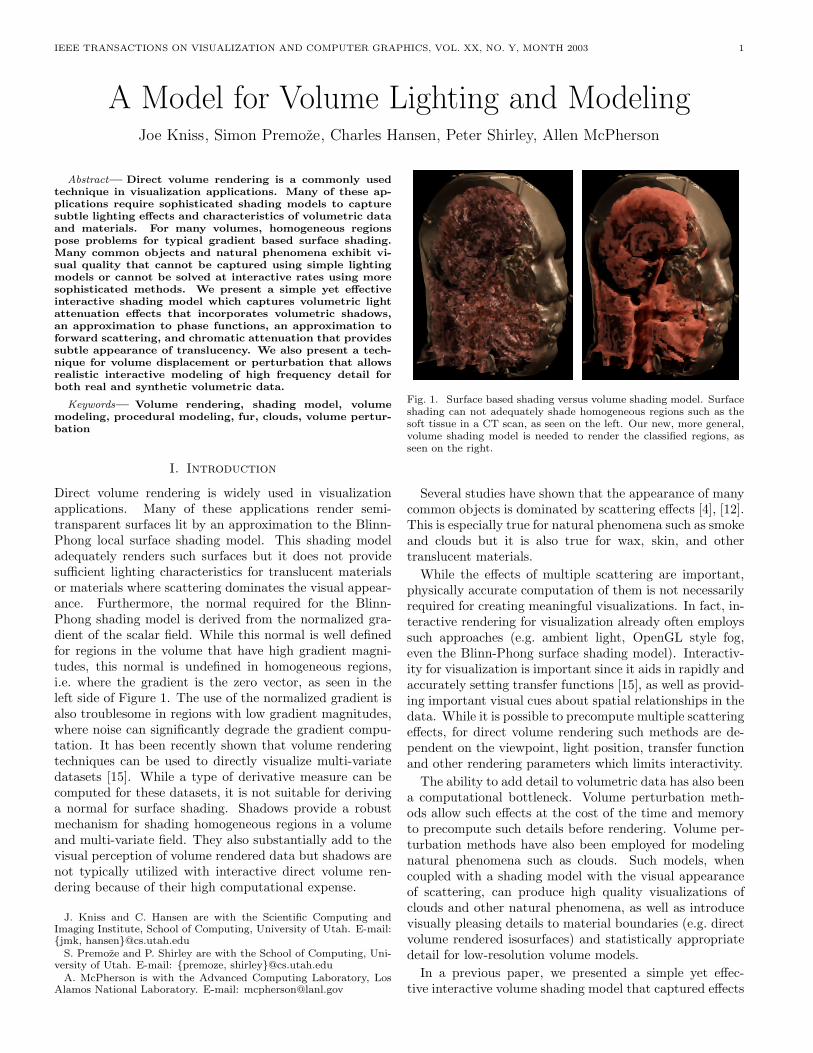
Fig. 1. Surface based shading versus volume shading model. Surfaceshading can not adequately shade homogeneous regions such as thesoft tissue in a CT scan, as seen on the left. Our new, more general,volume shading model is needed to render the classified regions, asseen on the right.

Several studies have shown that the appearance of manycommon objects is dominated by scattering effects [4], [12].This is especially true for natural phenomena such as smokeand clouds but it is also true for wax, skin, and othertranslucent materials.While the effects of multiple scattering are important,

physically accurate computation of them is not necessarilyrequired for creating meaningful visualizations. In fact, in-teractive rendering for visualization already often employssuch approaches (e.g. ambient light, OpenGL style fog,even the Blinn-Phong surface shading model). Interactiv-ity for visualization is important since it aids in rapidly andaccurately setting transfer functions [15], as well as provid-ing important visual cues about spatial relationships in thedata. While it is possible to precompute multiple scatteringeffects, for direct volume rendering such methods are de-pendent on the viewpoint, light position, transfer functionand other rendering parameters which limits interactivity.The ability to add detail to volumetric data has also been

a computational bottleneck. Volume perturbation meth-ods allow such effects at the cost of the time and memoryto precompute such details before rendering. Volume per-turbation methods have also been employed for modelingnatural phenomena such as clouds. Such models, whencoupled with a shading model with the visual appearanceof scattering, can produce high quality visualizations ofclouds and other natural phenomena, as well as introducevisually pleasing details to material boundaries (e.g. directvolume rendered isosurfaces) and statistically appropriatedetail for low-resolution volume models.In a previous paper, we presented a simple yet effec-

tive interactive volume shading model that captured effects


of volumetric light transport through translucent materi-als [16]. In this paper, we more thoroughly describe thatshading model and how it relates to the classical volumeshading. We also include forward peaked phase functioninto the model as well as other applications for volumeperturbation. This achieves a method for interactive vol-umetric light transport that can produce effects such asdirect lighting with phase angle influence, volumetric shad-ows, and a reasonable approximation of multiple scattering.This is shown in Figure 1. On the left is the standard sur-face shading of a CT scan of a head. On the right, renderedwith the same transfer function, is our improved shadingmodel. Leveraging the new light transport model allowsfor interactive volume modeling based on volumetric dis-placement or perturbation. This allows realistic interactivemodeling of clouds, height fields, as well as the introductionof details to volumetric data.In the next section, we introduce the problem of volume

shading and light transport and describe related work onvolume shading, scattering effects, as well as proceduralmodeling of clouds and surface detail. We then present thenew volumetric shading model which phenomenologicallymimics scattering and light attenuation through the vol-ume. Implementation details are discussed and an interac-tive volumetric perturbation method is introduced. Resultson a variety of volume data are also presented to demon-strate the effectiveness of these techniques.

II. Background

In this section we review previous work and give anoverview of volume shading equations.

A. Previous Work

Volume visualization for scalar fields was described inthree papers by Sabella, Drebin et al. and Levoy [29], [7],[18]. These methods describe volume shading incorporat-ing diffuse and specular shading by approximating the sur-face normal with the gradient of the 3D field. The volumerendering described in these seminal papers ignored scat-tering in favor of the fast approximation achieved by directlighting. Techniques for implementing these approachesto volume rendering have been successfully implementedin hardware providing interactive volume rendering of 3Dscalar fields [5], [25].Blinn was one of the first computer graphics researchers

to investigate volumetric scattering for computer graphicsand visualization applications. He presented a model forthe reflection and transmission of light through thin cloudsof particles based on probabilistic arguments and singlescattering approximation in which Fresnel effects were con-sidered [3]. Kajiya and von Herzen described a model forrendering arbitrary volume densities that included expen-sive multiple scattering computation. The radiative trans-port equation [13] cannot be solved analytically exceptfor some simple configurations. Expensive and sophisti-cated numerical methods must be employed to computethe radiance distribution to a desired accuracy. Finite ele-ment methods are commonly used to solve transport equa-

tions. Rushmeier presented zonal finite element methodsfor isotropic scattering in participating media [28], [27].Max et al. [20] used a one-dimensional scattering equationto compute the light transport in tree canopies by solving asystem of differential equations through the application ofthe Fourier transform. The method becomes expensive forforward peaked phase functions, as the hemisphere needs tobe more finely discretized. Spherical harmonics were alsoused by Kajiya and von Herzen [14] to compute anisotropicscattering as well as discrete ordinate methods (Languenouet al. [17]).Monte Carlo methods are robust and simple tech-

niques for solving light transport equation. Hanrahan andKrueger modeled scattering in layered surfaces with lineartransport theory and derived explicit formulas for backscat-tering and transmission [10]. The model is powerful androbust, but suffers from standard Monte Carlo problemssuch as slow convergence and noise. Pharr and Hanra-han described a mathematical framework [26] for solvingthe scattering equation in context of a variety of render-ing problems and also described a numerical Monte Carlosampling method. Jensen and Christensen described a two-pass approach to light transport in participating media [11]using a volumetric photon map. The method is simple,robust and efficient and it is able to handle arbitrary con-figurations. Dorsey et al. [6] described a method for fullvolumetric light transport inside stone structures using avolumetric photon map representation.Stam and Fiume showed the the often used diffusion

approximation can produce good results for scattering indense media [31]. Recently, Jensen et al. introduced com-putationally efficient analytical diffusion approximation tomultiple scattering [12], which is especially applicable forhomogeneous materials that exhibit considerable subsur-face light transport. The model does not appear to beeasily extendible to volumes with arbitrary optical prop-erties. Several other specialized approximations have beendeveloped for particular natural phenomena. Nishita etal. [22] presented an approximation to light transport insideclouds and Nishita [21] an overview of light transport andscattering methods for natural environments [21]. Theseapproximations are not generalizable for volume renderingapplications because of the limiting assumptions made inderiving the approximations.Max surveyed many optical models for volume rendering

applications [19] ranging from very simple to very complex,and accurate models that account for all interactions withinthe volume.Max [19] and Jensen et al. [12] clearly demonstrate that

the effects of multiple scattering and indirect illuminationare important for volume rendering applications. However,accurate simulations of full light transport are computa-tionally expensive and do not permit interactivity such aschanging the illumination or transfer function. Analyti-cal approximations exist, but they are severely restrictedby underlying assumptions, such as homogeneous opticalproperties and density, simple lighting or unrealistic bound-ary conditions. These analytical approximations cannot be


x0x1

x(s)

ωω

l

lll

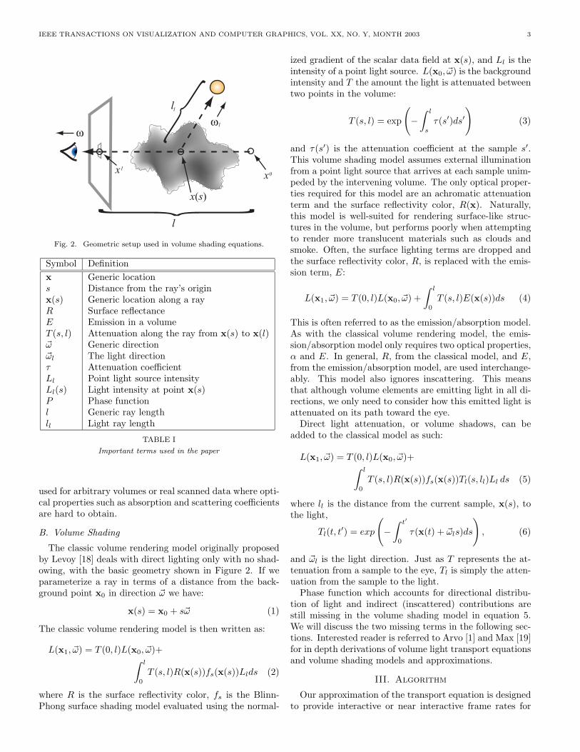
Fig. 2. Geometric setup used in volume shading equations.

Symbol Definitionx Generic locations Distance from the ray’s originx(s) Generic location along a rayR Surface reflectanceE Emission in a volumeT (s, l) Attenuation along the ray from x(s) to x(l)ω Generic directionωl The light directionτ Attenuation coefficientLl Point light source intensityLl(s) Light intensity at point x(s)P Phase functionl Generic ray lengthll Light ray length

TABLE I

Important terms used in the paper

used for arbitrary volumes or real scanned data where opti-cal properties such as absorption and scattering coefficientsare hard to obtain.

B. Volume Shading

The classic volume rendering model originally proposedby Levoy [18] deals with direct lighting only with no shad-owing, with the basic geometry shown in Figure 2. If weparameterize a ray in terms of a distance from the back-ground point x0 in direction ω we have:

x(s) = x0 + sω (1)

The classic volume rendering model is then written as:

L(x1, ω) = T (0, l)L(x0, ω)+∫ l

0

T (s, l)R(x(s))fs(x(s))Llds (2)

where R is the surface reflectivity color, fs is the Blinn-Phong surface shading model evaluated using the normal-

ized gradient of the scalar data field at x(s), and Ll is theintensity of a point light source. L(x0, ω) is the backgroundintensity and T the amount the light is attenuated betweentwo points in the volume:

T (s, l) = exp

(−∫ l

s

τ(s′)ds′)

(3)

and τ(s′) is the attenuation coefficient at the sample s′.This volume shading model assumes external illuminationfrom a point light source that arrives at each sample unim-peded by the intervening volume. The only optical proper-ties required for this model are an achromatic attenuationterm and the surface reflectivity color, R(x). Naturally,this model is well-suited for rendering surface-like struc-tures in the volume, but performs poorly when attemptingto render more translucent materials such as clouds andsmoke. Often, the surface lighting terms are dropped andthe surface reflectivity color, R, is replaced with the emis-sion term, E:

L(x1, ω) = T (0, l)L(x0, ω) +∫ l

0

T (s, l)E(x(s))ds (4)

This is often referred to as the emission/absorption model.As with the classical volume rendering model, the emis-sion/absorption model only requires two optical properties,α and E. In general, R, from the classical model, and E,from the emission/absorption model, are used interchange-ably. This model also ignores inscattering. This meansthat although volume elements are emitting light in all di-rections, we only need to consider how this emitted light isattenuated on its path toward the eye.Direct light attenuation, or volume shadows, can be

added to the classical model as such:

L(x1, ω) = T (0, l)L(x0, ω)+∫ l

0

T (s, l)R(x(s))fs(x(s))Tl(s, ll)Ll ds (5)

where ll is the distance from the current sample, x(s), tothe light,

Tl(t, t′) = exp

(−∫ t′

0

τ(x(t) + ωls)ds

), (6)

and ωl is the light direction. Just as T represents the at-tenuation from a sample to the eye, Tl is simply the atten-uation from the sample to the light.Phase function which accounts for directional distribu-

tion of light and indirect (inscattered) contributions arestill missing in the volume shading model in equation 5.We will discuss the two missing terms in the following sec-tions. Interested reader is referred to Arvo [1] and Max [19]for in depth derivations of volume light transport equationsand volume shading models and approximations.

III. Algorithm

Our approximation of the transport equation is designedto provide interactive or near interactive frame rates for


volume rendering when the transfer function, light direc-tion, or volume data are not static. Therefore, the lightintensity at each sample must be recomputed every frame.Our method for computing light transport is done in im-age space resolutions, allowing the computational complex-ity to match the level of detail. Since the computation oflight transport is decoupled from the resolution of the vol-ume data, we can also accurately compute lighting for vol-umes with high frequency displacement effects, which aredescribed in the second half of this section.

A. Direct Lighting

Our implementation can be best understood if we firstexamine the implementation of direct lighting. A bruteforce implementation of direct lighting, or volumetric shad-ows, can be accomplished by sending a shadow ray to-ward the light for each sample along the viewing ray toestimate the amount of extinction caused by the portionof the volume between that sample and the light. Thisalgorithm would have the computational complexity ofO(nm) ≡ O(n2) where n is the total number of samplestaken along each viewing ray, and m is the number of sam-ples taken along each shadow ray. In general, the algorithmwould be far to slow for interactive visualization. It is alsovery redundant since many of these shadow rays overlap.One possible solution would be to pre-compute lighting,by iteratively sampling the volume from the light’s pointof view, and storing the light intensities at each spatial po-sition in a so called “shadow volume”. While this approachreduces the computational complexity to O(n+m) ≡ O(n),it has a few obvious disadvantages. First, this method canrequire a significant amount of additional memory for stor-ing the shadow volume. When memory consumption andaccess times are a limiting factor, one must trade the resolu-tion of the shadow volume, and thus the resolution of directlighting computations, for reduced memory foot print andimproved access times. Another disadvantage of shadowvolume techniques is known as “attenuation leakage” thisis caused by the interpolation kernel used when accessingthe illumination in the shadow volume. If direct lightingcould be computed in lock step with the accumulation oflight for the eye, both integrals could be solved iterativelyin image space using 2D buffers, one for storing light fromthe eye’s point of view and another for the light sourcepoint of view. This can be accomplished using the methodof half angle slicing proposed for volume shadow compu-tation in [15], where the slice axis is halfway between thelight and view directions or halfway between the light andinverted view directions depending on the sign of the dotproduct of the two. The modification of the slicing axisprovides the ability to render each slice from the point ofview of both the observer and the light. Thereby achiev-ing the effect of a high resolution shadow map without therequirement of pre-computation and storage.This can be implemented very efficiently on graph-

ics hardware using texture based volume rendering tech-niques [33]. The approach requires an additional pass foreach slice, which updates the the light intensities for the

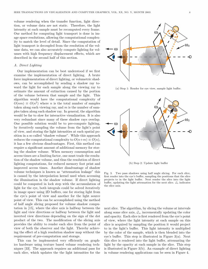
(a) Step 1: Render for eye view, sample light buffer.

(b) Step 2: Update light buffer

Fig. 3. Two pass shadows using half angle slicing. For each slice,first render into the eye’s buffer, sampling the positions that the sliceprojects to in the light buffer. Next render the slice into the lightbuffer, updating the light attenuation for the next slice. ωs indicatesthe slice axis.

next slice. The algorithm, by slicing the volume at intervalsalong some slice axis, ωs, incrementally updating the colorand opacity. Each slice is first rendered from the eye’s pointof view, where the light intensity at each sample on thisslice is acquired by sampling the position it would projectto in the light’s buffer. This light intensity is multipliedby the color of the sample, which is then blended into theeye’s buffer. This step is illustrated in Figure 3(a). Nextthis slice is rendered into the light buffer, attenuating thelight by the opacity at each sample in the slice. This stepis illustrated in Figure 3(b). An example of direct lightingin volume rendering applications can be seen in Figure 4.


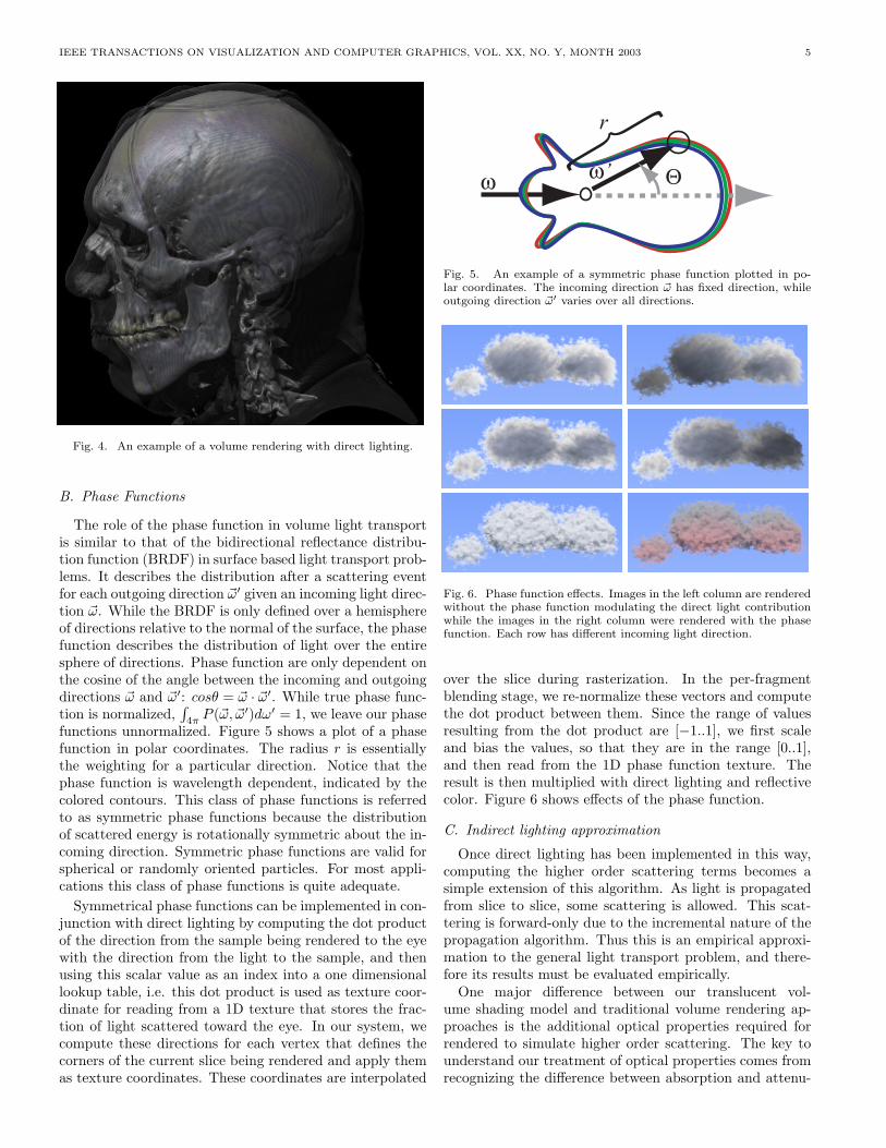
Fig. 4. An example of a volume rendering with direct lighting.

B. Phase Functions

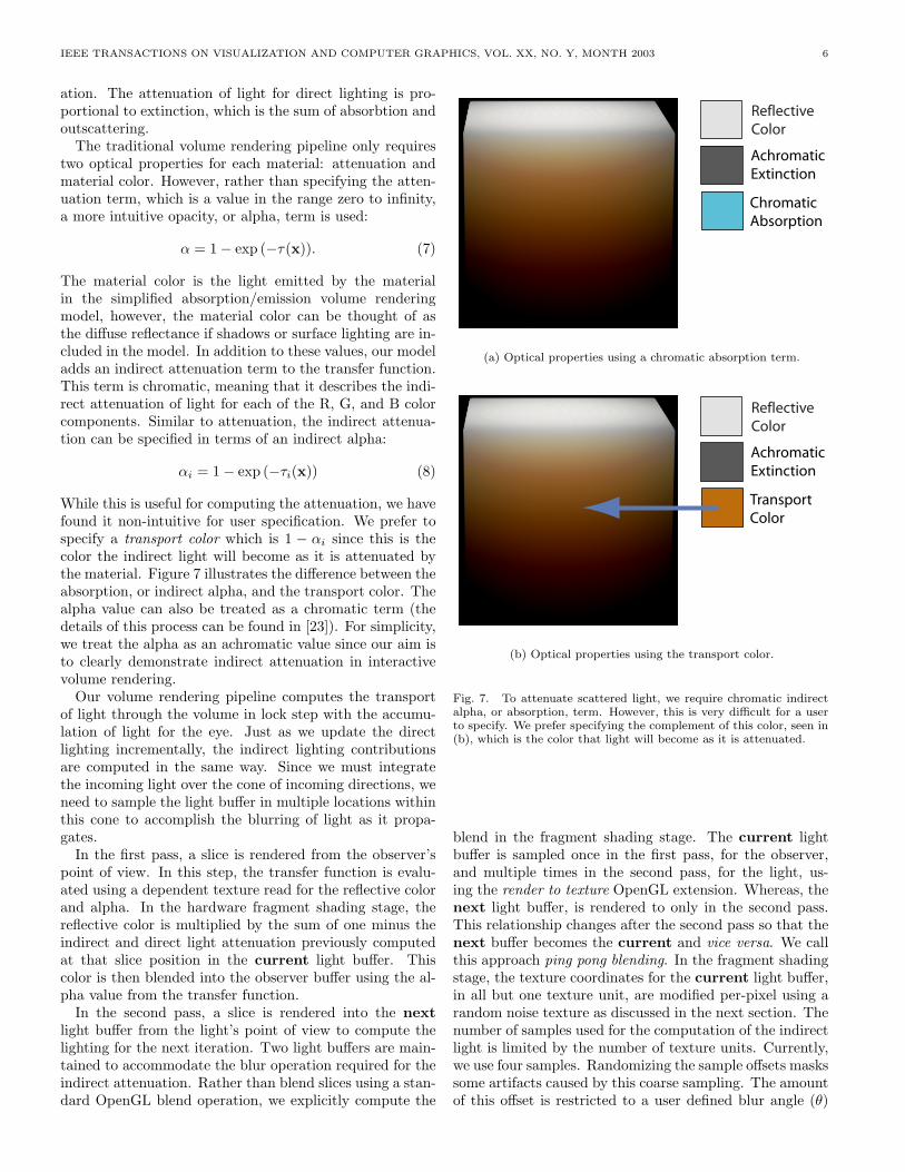
The role of the phase function in volume light transportis similar to that of the bidirectional reflectance distribu-tion function (BRDF) in surface based light transport prob-lems. It describes the distribution after a scattering eventfor each outgoing direction ω′ given an incoming light direc-tion ω. While the BRDF is only defined over a hemisphereof directions relative to the normal of the surface, the phasefunction describes the distribution of light over the entiresphere of directions. Phase function are only dependent onthe cosine of the angle between the incoming and outgoingdirections ω and ω′: cosθ = ω · ω′. While true phase func-tion is normalized,

∫4π

P (ω, ω′)dω′ = 1, we leave our phasefunctions unnormalized. Figure 5 shows a plot of a phasefunction in polar coordinates. The radius r is essentiallythe weighting for a particular direction. Notice that thephase function is wavelength dependent, indicated by thecolored contours. This class of phase functions is referredto as symmetric phase functions because the distributionof scattered energy is rotationally symmetric about the in-coming direction. Symmetric phase functions are valid forspherical or randomly oriented particles. For most appli-cations this class of phase functions is quite adequate.Symmetrical phase functions can be implemented in con-

junction with direct lighting by computing the dot productof the direction from the sample being rendered to the eyewith the direction from the light to the sample, and thenusing this scalar value as an index into a one dimensionallookup table, i.e. this dot product is used as texture coor-dinate for reading from a 1D texture that stores the frac-tion of light scattered toward the eye. In our system, wecompute these directions for each vertex that defines thecorners of the current slice being rendered and apply themas texture coordinates. These coordinates are interpolated

ω ω’ Θ

r

Fig. 5. An example of a symmetric phase function plotted in po-lar coordinates. The incoming direction ω has fixed direction, whileoutgoing direction ω′ varies over all directions.

Fig. 6. Phase function effects. Images in the left column are renderedwithout the phase function modulating the direct light contributionwhile the images in the right column were rendered with the phasefunction. Each row has different incoming light direction.

over the slice during rasterization. In the per-fragmentblending stage, we re-normalize these vectors and computethe dot product between them. Since the range of valuesresulting from the dot product are [−1..1], we first scaleand bias the values, so that they are in the range [0..1],and then read from the 1D phase function texture. Theresult is then multiplied with direct lighting and reflectivecolor. Figure 6 shows effects of the phase function.

C. Indirect lighting approximation

Once direct lighting has been implemented in this way,computing the higher order scattering terms becomes asimple extension of this algorithm. As light is propagatedfrom slice to slice, some scattering is allowed. This scat-tering is forward-only due to the incremental nature of thepropagation algorithm. Thus this is an empirical approxi-mation to the general light transport problem, and there-fore its results must be evaluated empirically.One major difference between our translucent vol-

ume shading model and traditional volume rendering ap-proaches is the additional optical properties required forrendered to simulate higher order scattering. The key tounderstand our treatment of optical properties comes fromrecognizing the difference between absorption and attenu-


ation. The attenuation of light for direct lighting is pro-portional to extinction, which is the sum of absorbtion andoutscattering.The traditional volume rendering pipeline only requires

two optical properties for each material: attenuation andmaterial color. However, rather than specifying the atten-uation term, which is a value in the range zero to infinity,a more intuitive opacity, or alpha, term is used:

α = 1− exp (−τ(x)). (7)

The material color is the light emitted by the materialin the simplified absorption/emission volume renderingmodel, however, the material color can be thought of asthe diffuse reflectance if shadows or surface lighting are in-cluded in the model. In addition to these values, our modeladds an indirect attenuation term to the transfer function.This term is chromatic, meaning that it describes the indi-rect attenuation of light for each of the R, G, and B colorcomponents. Similar to attenuation, the indirect attenua-tion can be specified in terms of an indirect alpha:

αi = 1− exp (−τi(x)) (8)

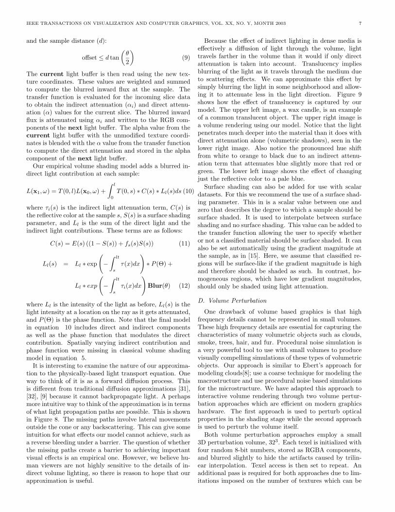
While this is useful for computing the attenuation, we havefound it non-intuitive for user specification. We prefer tospecify a transport color which is 1 − αi since this is thecolor the indirect light will become as it is attenuated bythe material. Figure 7 illustrates the difference between theabsorption, or indirect alpha, and the transport color. Thealpha value can also be treated as a chromatic term (thedetails of this process can be found in [23]). For simplicity,we treat the alpha as an achromatic value since our aim isto clearly demonstrate indirect attenuation in interactivevolume rendering.Our volume rendering pipeline computes the transport

of light through the volume in lock step with the accumu-lation of light for the eye. Just as we update the directlighting incrementally, the indirect lighting contributionsare computed in the same way. Since we must integratethe incoming light over the cone of incoming directions, weneed to sample the light buffer in multiple locations withinthis cone to accomplish the blurring of light as it propa-gates.In the first pass, a slice is rendered from the observer’s

point of view. In this step, the transfer function is evalu-ated using a dependent texture read for the reflective colorand alpha. In the hardware fragment shading stage, thereflective color is multiplied by the sum of one minus theindirect and direct light attenuation previously computedat that slice position in the current light buffer. Thiscolor is then blended into the observer buffer using the al-pha value from the transfer function.In the second pass, a slice is rendered into the next

light buffer from the light’s point of view to compute thelighting for the next iteration. Two light buffers are main-tained to accommodate the blur operation required for theindirect attenuation. Rather than blend slices using a stan-dard OpenGL blend operation, we explicitly compute the

ReflectiveColor

AchromaticExtinction

ChromaticAbsorption

(a) Optical properties using a chromatic absorption term.

ReflectiveColor

AchromaticExtinction

TransportColor

(b) Optical properties using the transport color.

Fig. 7. To attenuate scattered light, we require chromatic indirectalpha, or absorption, term. However, this is very difficult for a userto specify. We prefer specifying the complement of this color, seen in(b), which is the color that light will become as it is attenuated.

blend in the fragment shading stage. The current lightbuffer is sampled once in the first pass, for the observer,and multiple times in the second pass, for the light, us-ing the render to texture OpenGL extension. Whereas, thenext light buffer, is rendered to only in the second pass.This relationship changes after the second pass so that thenext buffer becomes the current and vice versa. We callthis approach ping pong blending. In the fragment shadingstage, the texture coordinates for the current light buffer,in all but one texture unit, are modified per-pixel using arandom noise texture as discussed in the next section. Thenumber of samples used for the computation of the indirectlight is limited by the number of texture units. Currently,we use four samples. Randomizing the sample offsets maskssome artifacts caused by this coarse sampling. The amountof this offset is restricted to a user defined blur angle (θ)


and the sample distance (d):

offset ≤ d tan(

θ

2

)(9)

The current light buffer is then read using the new tex-ture coordinates. These values are weighted and summedto compute the blurred inward flux at the sample. Thetransfer function is evaluated for the incoming slice datato obtain the indirect attenuation (αi) and direct attenu-ation (α) values for the current slice. The blurred inwardflux is attenuated using αi and written to the RGB com-ponents of the next light buffer. The alpha value from thecurrent light buffer with the unmodified texture coordi-nates is blended with the α value from the transfer functionto compute the direct attenuation and stored in the alphacomponent of the next light buffer.Our empirical volume shading model adds a blurred in-

direct light contribution at each sample:

L(x1, ω) = T (0, l)L(x0, ω) +∫ l

0

T (0, s) ∗ C(s) ∗ Ll(s)ds (10)

where τi(s) is the indirect light attenuation term, C(s) isthe reflective color at the sample s, S(s) is a surface shadingparameter, and Ll is the sum of the direct light and theindirect light contributions. These terms are as follows:

C(s) = E(s) ((1− S(s)) + fs(s)S(s)) (11)

Ll(s) = Ll ∗ exp(−∫ lt

s

τ(x)dx

)∗ P (Θ) +

Ll ∗ exp

(−∫ lt

s

τi(x)dx

)Blur(θ) (12)

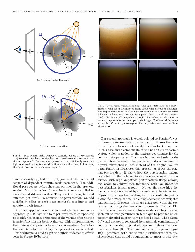
where Ll is the intensity of the light as before, Ll(s) is thelight intensity at a location on the ray as it gets attenuated,and P (Θ) is the phase function. Note that the final modelin equation 10 includes direct and indirect componentsas well as the phase function that modulates the directcontribution. Spatially varying indirect contribution andphase function were missing in classical volume shadingmodel in equation 5.It is interesting to examine the nature of our approxima-

tion to the physically-based light transport equation. Oneway to think of it is as a forward diffusion process. Thisis different from traditional diffusion approximations [31],[32], [9] because it cannot backpropagate light. A perhapsmore intuitive way to think of the approximation is in termsof what light propagation paths are possible. This is shownin Figure 8. The missing paths involve lateral movementsoutside the cone or any backscattering. This can give someintuition for what effects our model cannot achieve, such asa reverse bleeding under a barrier. The question of whetherthe missing paths create a barrier to achieving importantvisual effects is an empirical one. However, we believe hu-man viewers are not highly sensitive to the details of in-direct volume lighting, so there is reason to hope that ourapproximation is useful.

Because the effect of indirect lighting in dense media iseffectively a diffusion of light through the volume, lighttravels farther in the volume than it would if only directattenuation is taken into account. Translucency impliesblurring of the light as it travels through the medium dueto scattering effects. We can approximate this effect bysimply blurring the light in some neighborhood and allow-ing it to attenuate less in the light direction. Figure 9shows how the effect of translucency is captured by ourmodel. The upper left image, a wax candle, is an exampleof a common translucent object. The upper right image isa volume rendering using our model. Notice that the lightpenetrates much deeper into the material than it does withdirect attenuation alone (volumetric shadows), seen in thelower right image. Also notice the pronounced hue shiftfrom white to orange to black due to an indirect attenu-ation term that attenuates blue slightly more that red orgreen. The lower left image shows the effect of changingjust the reflective color to a pale blue.Surface shading can also be added for use with scalar

datasets. For this we recommend the use of a surface shad-ing parameter. This in is a scalar value between one andzero that describes the degree to which a sample should besurface shaded. It is used to interpolate between surfaceshading and no surface shading. This value can be added tothe transfer function allowing the user to specify whetheror not a classified material should be surface shaded. It canalso be set automatically using the gradient magnitude atthe sample, as in [15]. Here, we assume that classified re-gions will be surface-like if the gradient magnitude is highand therefore should be shaded as such. In contrast, ho-mogeneous regions, which have low gradient magnitudes,should only be shaded using light attenuation.

D. Volume Perturbation

One drawback of volume based graphics is that highfrequency details cannot be represented in small volumes.These high frequency details are essential for capturing thecharacteristics of many volumetric objects such as clouds,smoke, trees, hair, and fur. Procedural noise simulation isa very powerful tool to use with small volumes to producevisually compelling simulations of these types of volumetricobjects. Our approach is similar to Ebert’s approach formodeling clouds[8]; use a coarse technique for modeling themacrostructure and use procedural noise based simulationsfor the microstructure. We have adapted this approach tointeractive volume rendering through two volume pertur-bation approaches which are efficient on modern graphicshardware. The first approach is used to perturb opticalproperties in the shading stage while the second approachis used to perturb the volume itself.Both volume perturbation approaches employ a small

3D perturbation volume, 323. Each texel is initialized withfour random 8-bit numbers, stored as RGBA components,and blurred slightly to hide the artifacts caused by trilin-ear interpolation. Texel access is then set to repeat. Anadditional pass is required for both approaches due to lim-itations imposed on the number of textures which can be


x(s)

Ω

(a) General Light Transport

x(s)

Θ

ω lΩ(ω,Θ)

(b) Our Approximation

Fig. 8. Top, general light transport scenario, where at any samplex(s) we must consider incoming light scattered from all directions overthe unit sphere Ω. Bottom, our approximation, which only considerslight scattered in the forward direction within the cone of directions,the light direction ωl with apex angle Θ.

simultaneously applied to a polygon, and the number ofsequential dependent texture reads permitted. The addi-tional pass occurs before the steps outlined in the previoussection. Multiple copies of the noise texture are applied toeach slice at different scales. They are then weighted andsummed per pixel. To animate the perturbation, we adda different offset to each noise texture’s coordinates andupdate it each frame.Our first approach is similar to Ebert’s lattice based noise

approach [8]. It uses the four per-pixel noise componentsto modify the optical properties of the volume after the thetransfer function has been evaluated. This approach makesthe materials appear to have inhomogeneities. We allowthe user to select which optical properties are modified.This technique is used to get the subtle iridescence effectsseen in Figure 10(bottom).

Fig. 9. Translucent volume shading. The upper left image is a photo-graph of wax block illuminated from above with a focused flashlight.The upper right image is a volume rendering with a white reflectivecolor and a desaturated orange transport color (1− indirect attenua-tion). The lower left image has a bright blue reflective color and thesame transport color as the upper right image. The lower right imageshows the effect of light transport that only takes into account directattenuation.

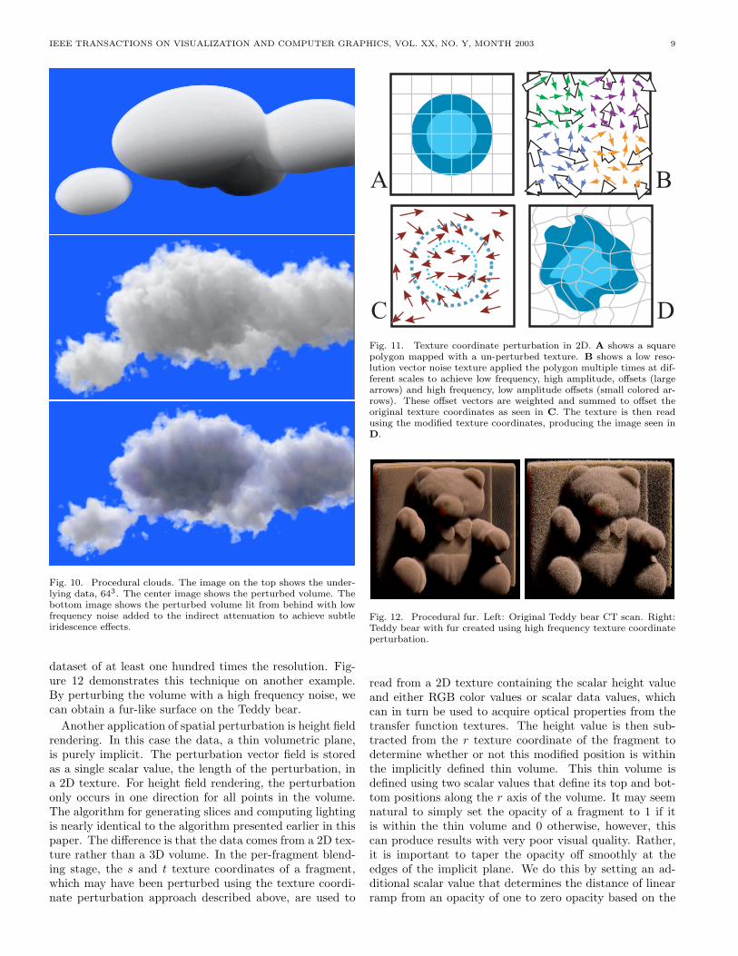
Our second approach is closely related to Peachey’s vec-tor based noise simulation technique [8]. It uses the noiseto modify the location of the data access for the volume.In this case three components of the noise texture form avector, which is added to the texture coordinates for thevolume data per pixel. The data is then read using a de-pendent texture read. The perturbed data is rendered toa pixel buffer that is used instead of the original volumedata. Figure 11 illustrates this process. A shows the orig-inal texture data. B shows how the perturbation textureis applied to the polygon twice, once to achieve low fre-quency with high amplitude perturbations (large arrows)and again to achieve high frequency with low amplitudeperturbations (small arrows). Notice that the high fre-quency content is created by allowing the texture to repeat.Figure 11 C shows the resulting texture coordinate pertur-bation field when the multiple displacements are weightedand summed. D shows the image generated when the tex-ture is read using the perturbed texture coordinates. Fig-ure 10 shows how a coarse volume model can be combinedwith our volume perturbation technique to produce an ex-tremely detailed interactively rendered cloud. The original643 voxel dataset is generated from a simple combination ofvolumetric blended implicit ellipses and defines the cloudmacrostructure [8]. The final rendered image in Figure10(c), produced with our volume perturbation technique,shows detail that would be equivalent to unperturbed voxel


Fig. 10. Procedural clouds. The image on the top shows the under-lying data, 643. The center image shows the perturbed volume. Thebottom image shows the perturbed volume lit from behind with lowfrequency noise added to the indirect attenuation to achieve subtleiridescence effects.

dataset of at least one hundred times the resolution. Fig-ure 12 demonstrates this technique on another example.By perturbing the volume with a high frequency noise, wecan obtain a fur-like surface on the Teddy bear.Another application of spatial perturbation is height field

rendering. In this case the data, a thin volumetric plane,is purely implicit. The perturbation vector field is storedas a single scalar value, the length of the perturbation, ina 2D texture. For height field rendering, the perturbationonly occurs in one direction for all points in the volume.The algorithm for generating slices and computing lightingis nearly identical to the algorithm presented earlier in thispaper. The difference is that the data comes from a 2D tex-ture rather than a 3D volume. In the per-fragment blend-ing stage, the s and t texture coordinates of a fragment,which may have been perturbed using the texture coordi-nate perturbation approach described above, are used to

A B

C DFig. 11. Texture coordinate perturbation in 2D. A shows a squarepolygon mapped with a un-perturbed texture. B shows a low reso-lution vector noise texture applied the polygon multiple times at dif-ferent scales to achieve low frequency, high amplitude, offsets (largearrows) and high frequency, low amplitude offsets (small colored ar-rows). These offset vectors are weighted and summed to offset theoriginal texture coordinates as seen in C. The texture is then readusing the modified texture coordinates, producing the image seen inD.

Fig. 12. Procedural fur. Left: Original Teddy bear CT scan. Right:Teddy bear with fur created using high frequency texture coordinateperturbation.

read from a 2D texture containing the scalar height valueand either RGB color values or scalar data values, whichcan in turn be used to acquire optical properties from thetransfer function textures. The height value is then sub-tracted from the r texture coordinate of the fragment todetermine whether or not this modified position is withinthe implicitly defined thin volume. This thin volume isdefined using two scalar values that define its top and bot-tom positions along the r axis of the volume. It may seemnatural to simply set the opacity of a fragment to 1 if itis within the thin volume and 0 otherwise, however, thiscan produce results with very poor visual quality. Rather,it is important to taper the opacity off smoothly at theedges of the implicit plane. We do this by setting an ad-ditional scalar value that determines the distance of linearramp from an opacity of one to zero opacity based on the


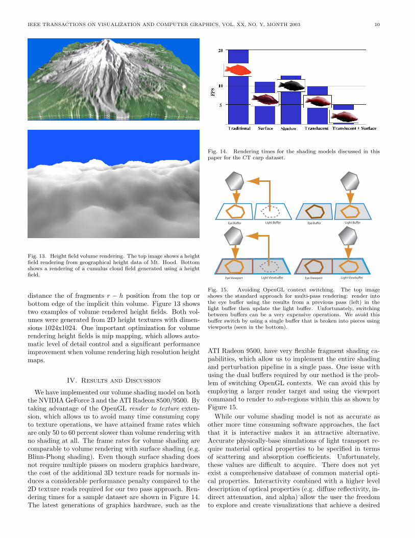
Fig. 13. Height field volume rendering. The top image shows a heightfield rendering from geographical height data of Mt. Hood. Bottomshows a rendering of a cumulus cloud field generated using a heightfield.

distance the of fragments r − h position from the top orbottom edge of the implicit thin volume. Figure 13 showstwo examples of volume rendered height fields. Both vol-umes were generated from 2D height textures with dimen-sions 1024x1024. One important optimization for volumerendering height fields is mip mapping, which allows auto-matic level of detail control and a significant performanceimprovement when volume rendering high resolution heightmaps.

IV. Results and Discussion

We have implemented our volume shading model on boththe NVIDIA GeForce 3 and the ATI Radeon 8500/9500. Bytaking advantage of the OpenGL render to texture exten-sion, which allows us to avoid many time consuming copyto texture operations, we have attained frame rates whichare only 50 to 60 percent slower than volume rendering withno shading at all. The frame rates for volume shading arecomparable to volume rendering with surface shading (e.g.Blinn-Phong shading). Even though surface shading doesnot require multiple passes on modern graphics hardware,the cost of the additional 3D texture reads for normals in-duces a considerable performance penalty compared to the2D texture reads required for our two pass approach. Ren-dering times for a sample dataset are shown in Figure 14.The latest generations of graphics hardware, such as the

Fig. 14. Rendering times for the shading models discussed in thispaper for the CT carp dataset.

Eye Buffer Light Buffer Eye Buffer Light Buffer

Eye Viewport Light Viewbuffer Eye Viewport Light Viewbuffer

Fig. 15. Avoiding OpenGL context switching. The top imageshows the standard approach for multi-pass rendering: render intothe eye buffer using the results from a previous pass (left) in thelight buffer then update the light buffer. Unfortunately, switchingbetween buffers can be a very expensive operations. We avoid thisbuffer switch by using a single buffer that is broken into pieces usingviewports (seen in the bottom).

ATI Radeon 9500, have very flexible fragment shading ca-pabilities, which allow us to implement the entire shadingand perturbation pipeline in a single pass. One issue withusing the dual buffers required by our method is the prob-lem of switching OpenGL contexts. We can avoid this byemploying a larger render target and using the viewportcommand to render to sub-regions within this as shown byFigure 15.While our volume shading model is not as accurate as

other more time consuming software approaches, the factthat it is interactive makes it an attractive alternative.Accurate physically-base simulations of light transport re-quire material optical properties to be specified in termsof scattering and absorption coefficients. Unfortunately,these values are difficult to acquire. There does not yetexist a comprehensive database of common material opti-cal properties. Interactivity combined with a higher leveldescription of optical properties (e.g. diffuse reflectivity, in-direct attenuation, and alpha) allow the user the freedomto explore and create visualizations that achieve a desired


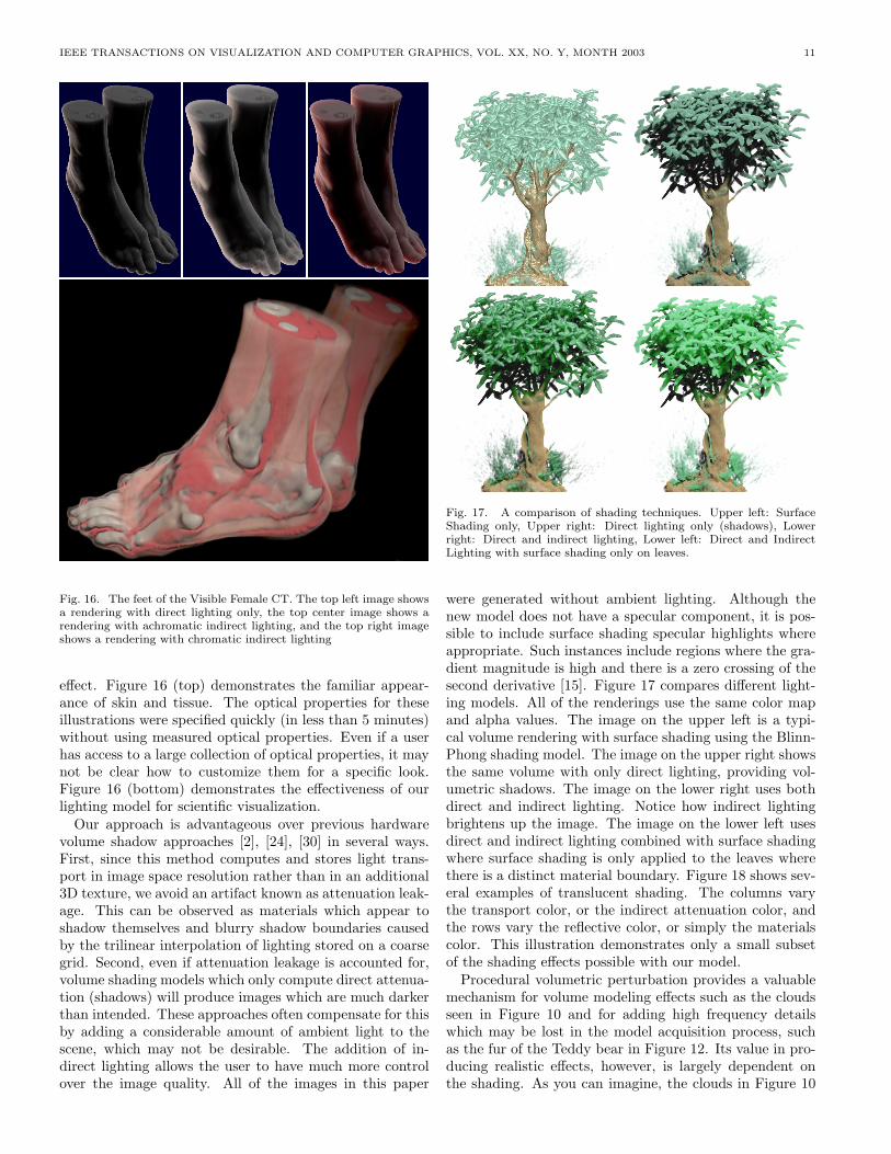
Fig. 16. The feet of the Visible Female CT. The top left image showsa rendering with direct lighting only, the top center image shows arendering with achromatic indirect lighting, and the top right imageshows a rendering with chromatic indirect lighting

effect. Figure 16 (top) demonstrates the familiar appear-ance of skin and tissue. The optical properties for theseillustrations were specified quickly (in less than 5 minutes)without using measured optical properties. Even if a userhas access to a large collection of optical properties, it maynot be clear how to customize them for a specific look.Figure 16 (bottom) demonstrates the effectiveness of ourlighting model for scientific visualization.Our approach is advantageous over previous hardware

volume shadow approaches [2], [24], [30] in several ways.First, since this method computes and stores light trans-port in image space resolution rather than in an additional3D texture, we avoid an artifact known as attenuation leak-age. This can be observed as materials which appear toshadow themselves and blurry shadow boundaries causedby the trilinear interpolation of lighting stored on a coarsegrid. Second, even if attenuation leakage is accounted for,volume shading models which only compute direct attenua-tion (shadows) will produce images which are much darkerthan intended. These approaches often compensate for thisby adding a considerable amount of ambient light to thescene, which may not be desirable. The addition of in-direct lighting allows the user to have much more controlover the image quality. All of the images in this paper

Fig. 17. A comparison of shading techniques. Upper left: SurfaceShading only, Upper right: Direct lighting only (shadows), Lowerright: Direct and indirect lighting, Lower left: Direct and IndirectLighting with surface shading only on leaves.

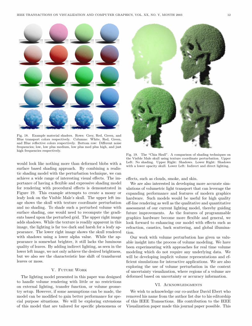
were generated without ambient lighting. Although thenew model does not have a specular component, it is pos-sible to include surface shading specular highlights whereappropriate. Such instances include regions where the gra-dient magnitude is high and there is a zero crossing of thesecond derivative [15]. Figure 17 compares different light-ing models. All of the renderings use the same color mapand alpha values. The image on the upper left is a typi-cal volume rendering with surface shading using the Blinn-Phong shading model. The image on the upper right showsthe same volume with only direct lighting, providing vol-umetric shadows. The image on the lower right uses bothdirect and indirect lighting. Notice how indirect lightingbrightens up the image. The image on the lower left usesdirect and indirect lighting combined with surface shadingwhere surface shading is only applied to the leaves wherethere is a distinct material boundary. Figure 18 shows sev-eral examples of translucent shading. The columns varythe transport color, or the indirect attenuation color, andthe rows vary the reflective color, or simply the materialscolor. This illustration demonstrates only a small subsetof the shading effects possible with our model.Procedural volumetric perturbation provides a valuable

mechanism for volume modeling effects such as the cloudsseen in Figure 10 and for adding high frequency detailswhich may be lost in the model acquisition process, suchas the fur of the Teddy bear in Figure 12. Its value in pro-ducing realistic effects, however, is largely dependent onthe shading. As you can imagine, the clouds in Figure 10


Fig. 18. Example material shaders. Rows: Grey, Red, Green, andBlue transport colors respectively. Columns: White, Red, Green,and Blue reflective colors respectively. Bottom row: Different noisefrequencies; low, low plus medium, low plus med plus high, and justhigh frequencies respectively.

would look like nothing more than deformed blobs with asurface based shading approach. By combining a realis-tic shading model with the perturbation technique, we canachieve a wide range of interesting visual effects. The im-portance of having a flexible and expressive shading modelfor rendering with procedural effects is demonstrated inFigure 19. This example attempts to create a mossy orleafy look on the Visible Male’s skull. The upper left im-age shows the skull with texture coordinate perturbationand no shading. To shade such a perturbed volume withsurface shading, one would need to recompute the gradi-ents based upon the perturbed grid. The upper right imageadds shadows. While the texture is readily apparent in thisimage, the lighting is far too dark and harsh for a leafy ap-pearance. The lower right image shows the skull renderedwith shadows using a lower alpha value. While the ap-pearance is somewhat brighter, it still lacks the luminousquality of leaves. By adding indirect lighting, as seen in thelower left image, we not only achieve the desired brightness,but we also see the characteristic hue shift of translucentleaves or moss.

V. Future Work

The lighting model presented in this paper was designedto handle volume rendering with little or no restrictionson external lighting, transfer function, or volume geome-try setup. However, if some assumptions can be made, themodel can be modified to gain better performance for spe-cial purpose situations. We will be exploring extensionsof this model that are tailored for specific phenomena or

Fig. 19. The “Chia Skull”. A comparison of shading techniques onthe Visible Male skull using texture coordinate perturbation. UpperLeft: No shading. Upper Right: Shadows. Lower Right: Shadowswith a lower opacity skull. Lower Left: Indirect and direct lighting.

effects, such as clouds, smoke, and skin.We are also interested in developing more accurate sim-

ulations of volumetric light transport that can leverage theexpanding performance and features of modern graphicshardware. Such models would be useful for high qualityoff-line rendering as well as the qualitative and quantitativeassessment of our current lighting model, thereby guidingfuture improvements. As the features of programmablegraphics hardware become more flexible and general, welook forward to enhancing our model with effects such asrefraction, caustics, back scattering, and global illumina-tion.Our work with volume perturbation has given us valu-

able insight into the process of volume modeling. We havebeen experimenting with approaches for real time volumemodeling which do not require any underlying data. Wewill be developing implicit volume representations and ef-ficient simulations for interactive applications. We are alsoexploring the use of volume perturbation in the contextof uncertainty visualization, where regions of a volume aredeformed based on uncertainty or accuracy information.

VI. Acknowledgments

We wish to acknowledge our co-author David Ebert whoremoved his name from the author list due to his editorshipof this IEEE Transactions. His contribution to the IEEEVisualization paper made this journal paper possible. This


material is based upon work supported by the NationalScience Foundation under Grants: NSF ACI-0081581, NSFACI-0121288, NSF IIS-0098443, NSF ACI-9978032, NSFMRI-9977218, NSF ACR-9978099, and the DOE VIEWSprogram.

References

[1] Arvo, J. Transfer equations in global illumination. Global Illu-mination, SIGGRAPH ‘93 Course Notes, August 1993.

[2] Behrens, U., and Ratering, R. Adding Shadows to a Texture-Based Volume Renderer. In 1998 Volume Visualization Sympo-sium (1998), pp. 39–46.

[3] Blinn, J. F. Light reflection functions for simulation of cloudsand dusty surfaces. In Proceedings of SIGGRAPH (1982),pp. 21–29.

[4] Bohren, C. F. Multiple scattering of light and some of itsobservable consequences. American Journal of Physics 55, 6(June 1987), 524–533.

[5] Cabral, B., Cam, N., and Foran, J. Accelerated volume ren-dering and tomographic reconstruction using texture mappinghardware. In 1994 Symposium on Volume Visualization (Oct.1994), A. Kaufman and W. Krueger, Eds., ACM SIGGRAPH,pp. 91–98. ISBN 0-89791-741-3.

[6] Dorsey, J., Edelman, A., Jensen, H. W., Legakis, J., and

Pedersen, H. Modeling and rendering of weathered stone. InProceedings of SIGGRAPH 1999 (August 1999), pp. 225–234.

[7] Drebin, R. A., Carpenter, L., and Hanrahan, P. Volumerendering. In Computer Graphics (SIGGRAPH ’88 Proceedings)(Aug. 1988), J. Dill, Ed., vol. 22, pp. 65–74.

[8] Ebert, D., Musgrave, F. K., Peachey, D., Perlin, K., and

Worley, S. Texturing and Modeling: A Procedural Approach.Academic Press, July 1998.

[9] Farrell, T. J., Patterson, M. S., and Wilson, B. C. Adiffusion theory model of spatially resolved, steady-state diffusereflectance for the non-invasive determination of tissue opticalproperties in vivo. Medical Physics 19 (1992), 879–888.

[10] Hanrahan, P., and Krueger, W. Reflection from layered sur-faces due to subsurface scattering. In Computer Graphics (SIG-GRAPH ’93 Proceedings) (Aug. 1993), J. T. Kajiya, Ed., vol. 27,pp. 165–174.

[11] Jensen, H. W., and Christensen, P. H. Efficient simulationof light transport in scenes with participating media using pho-ton maps. In Proceedings of SIGGRAPH 98 (Orlando, Florida,July 1998), Computer Graphics Proceedings, Annual ConferenceSeries, pp. 311–320.

[12] Jensen, H. W., Marschner, S. R., Levoy, M., and Hanra-

han, P. A practical model for subsurface light transport. In Pro-ceedings of SIGGRAPH 2001 (August 2001), Computer Graph-ics Proceedings, Annual Conference Series, pp. 511–518.

[13] Kajiya, J. T. The rendering equation. In Computer Graphics(SIGGRAPH ’86 Proceedings) (Aug. 1986), D. C. Evans andR. J. Athay, Eds., vol. 20, pp. 143–150.

[14] Kajiya, J. T., and Von Herzen, B. P. Ray tracing volumedensities. In Computer Graphics (SIGGRAPH ’84 Proceedings)(July 1984), H. Christiansen, Ed., vol. 18, pp. 165–174.

[15] Kniss, J., Kindlmann, G., and Hansen, C. Multi-DimensionalTransfer Functions for Interactive Volume Rendering. TVCG 8,4 (July 2002), 270–285.

[16] Kniss, J., Premoze, S., Hansen, C., and Ebert, D. InteractiveVolume Light Transport and Procedural Modeling. In IEEEVisualization 2002 (2002), pp. 109–116.

[17] Languenou, E., Bouatouch, K., and Chelle, M. Global illu-mination in presence of participating media with general proper-ties. In Fifth Eurographics Workshop on Rendering (Darmstadt,Germany, June 1994), pp. 69–85.

[18] Levoy, M. Display of surfaces from volume data. IEEE Com-puter Graphics & Applications 8, 5 (1988), 29–37.

[19] Max, N. Optical models for direct volume rendering. IEEETransactions on Visualization and Computer Graphics 1, 2(June 1995), 99–108.

[20] Max, N., Mobley, C., Keating, B., and Wu, E. Plane-parallelradiance transport for global illumination in vegetation. In Eu-rographics Rendering Workshop 1997 (New York City, NY, June1997), J. Dorsey and P. Slusallek, Eds., Eurographics, SpringerWien, pp. 239–250. ISBN 3-211-83001-4.

[21] Nishita, T. Light scattering models for the realistic rendering.In Proceedings of the Eurographics (1998), pp. 1–10.

[22] Nishita, T., Nakamae, E., and Dobashi, Y. Display of cloudsand snow taking into account multiple anisotropic scatteringand sky light. In SIGGRAPH 96 Conference Proceedings (Aug.1996), H. Rushmeier, Ed., Annual Conference Series, ACM SIG-GRAPH, Addison Wesley, pp. 379–386. held in New Orleans,Louisiana, 04-09 August 1996.

[23] Noordmans, H. J., van der Voort, H. T., and Smeulders,

A. W. Spectral Volume Rendering. IEEE Transactions on Vi-sualization and Computer Graphics 6, 3 (July-September 2000).

[24] Nulkar, M., and Mueller, K. Splatting With Shadows. InVolume Graphics 2001 (2001), pp. 35–49.

[25] Pfister, H., Hardenbergh, J., Knittel, J., Lauer, H., and

Seiler, L. The VolumePro Real-Time Ray-Casting System . InACM Computer Graphics (SIGGRAPH ’99 Proceedings) (Au-gust 1999), pp. 251–260.

[26] Pharr, M., and Hanrahan, P. M. Monte carlo evaluation ofnon-linear scattering equations for subsurface reflection. In Pro-ceedings of SIGGRAPH 2000 (July 2000), Computer GraphicsProceedings, Annual Conference Series, pp. 75–84.

[27] Rushmeier, H. E. Realistic Image Synthesis for Scenes with Ra-diatively Participating Media. Ph.d. thesis, Cornell University,1988.

[28] Rushmeier, H. E., and Torrance, K. E. The zonal methodfor calculating light intensities in the presence of a participatingmedium. In Computer Graphics (SIGGRAPH ’87 Proceedings)(July 1987), M. C. Stone, Ed., vol. 21, pp. 293–302.

[29] Sabella, P. A rendering algorithm for visualizing 3D scalarfields. In Computer Graphics (SIGGRAPH ’88 Proceedings)(Aug. 1988), J. Dill, Ed., vol. 22, pp. 51–58.

[30] Stam, J. Stable Fluids. In Siggraph 99 (1999), pp. 121–128.[31] Stam, J., and Fiume, E. Depicting fire and other gaseous phe-

nomena using diffusion processes. In SIGGRAPH 95 ConferenceProceedings (Aug. 1995), R. Cook, Ed., Annual Conference Se-ries, ACM SIGGRAPH, Addison Wesley, pp. 129–136. held inLos Angeles, California, 06-11 August 1995.

[32] Wang, L. V. Rapid modelling of diffuse reflectance of light inturbid slabs. J. Opt. Soc. Am. A 15, 4 (1998), 936–944.

[33] Wilson, O., Gelder, A. V., and Wilhelms, J. Direct Vol-ume Rendering via 3D Textures. Tech. Rep. UCSC-CRL-94-19,University of California at Santa Cruz, June 1994.

Documents

IEEE TRANSACTIONS ON VISUALIZATION AND COMPUTER …shirley/papers/volshade.pdf · IEEE TRANSACTIONS ON VISUALIZATION AND COMPUTER GRAPHICS, VOL. XX, NO. Y, MONTH 2003 1 A Model for