422 IEEE TRANSACTIONS ON VISUALIZATION AND COMPUTER

A Streaming Narrow-Band Algorithm:Interactive Computation and Visualization

of Level SetsAaron E. Lefohn, Student Member, IEEE, Joe M. Kniss, Student Member, IEEE,

Charles D. Hansen, Member, IEEE, and Ross T. Whitaker, Member, IEEE

Abstract—Deformable isosurfaces, implemented with level-set methods, have demonstrated a great potential in visualization and

computer graphics for applications such as segmentation, surface processing, and physically-based modeling. Their usefulness has

been limited, however, by their high computational cost and reliance on significant parameter tuning. This paper presents a solution to

these challenges by describing graphics processor (GPU) based algorithms for solving and visualizing level-set solutions at interactive

rates. The proposed solution is based on a new, streaming implementation of the narrow-band algorithm. The new algorithm packs the

level-set isosurface data into 2D texture memory via a multidimensional virtual memory system. As the level set moves, this texture-

based representation is dynamically updated via a novel GPU-to-CPU message passing scheme. By integrating the level-set solver

with a real-time volume renderer, a user can visualize and intuitively steer the level-set surface as it evolves. We demonstrate the

capabilities of this technology for interactive volume segmentation and visualization.

Index Terms—Deformable models, image segmentation, volume visualization, GPU, level sets, streaming computation, virtual

memory.

�

1 INTRODUCTION

LEVEL-SET methods [1] rely on partial differential equa-tions (PDEs) to model deforming isosurfaces. These

methods have applications in a wide range of fields such asvisualization, scientific computing, computer graphics, andcomputer vision [2], [3]. Applications in visualizationinclude volume segmentation [4], surface processing [5],and surface reconstruction [6].

The use of level sets in visualization can be problematic.Level sets are relatively slow to compute and they typicallyintroduce several free parameters that control the surfacedeformation and the quality of the results. Setting these freeparameters can be difficult because, inmany scenarios, a usermust wait minutes or hours to observe the results of aparameter change. Although efforts have been made to takeadvantage of the sparse nature of the computation, the mosthighly optimized solvers are still far from interactive. Thispaper proposes a solution to the above problems bymappingthe level-set PDE solver to a commodity graphics processor.

While the proposed technology has a wide range of useswithin visualization and elsewhere, this paper focuses on aparticular application: the analysis and visualization ofvolume data. By accelerating the PDE solver to interactiverates and coupling it to a real-time volume renderer, it ispossible to visualize and steer the computation of a level-setsurface as it moves toward interesting regions within avolume. The volume renderer provides visual context for

the evolving level set due to the global nature of the transferfunction’s opacity and color assignment. Also, the results ofa level-set segmentation can specify a region-of-interest forthe volume renderer [7].

The main contributions of this paper are:

. An integrated system demonstrating that level-setcomputations can be intuitively controlled by cou-pling a real-time volume renderer with an inter-active solver.

. A GPU-based 3D level-set solver that is approxi-mately 15 times faster than previous optimizedsolutions.

. A multidimensional virtual memory scheme forGPU texture memory that supports computationon time-dependent, sparse data.

. Real-time volume rendering directly from a packed,2D texture format. The technique also enablesvolume rendering from a data set represented as asingle set of 2D slices.

. A message passing scheme between the GPU andCPU that uses automatic mipmap generation tocreate compact, encoded messages.

. Efficient computation of a volumetric distance trans-form on the GPU.

2 BACKGROUND AND RELATED WORK

2.1 Level Sets

This paper describes a new solver for an implicit repre-sentation of deformable surface models called the methodof level sets [1]. The use of level sets has been widelydocumented in the visualization literature and severalworks give comprehensive reviews of the method and the

422 IEEE TRANSACTIONS ON VISUALIZATION AND COMPUTER GRAPHICS, VOL. 10, NO. 4, JULY/AUGUST 2004

. The authors are with the School of Computing, 50 S. Central CampusDrive, Rm 3190 MEB, University of Utah, Salt Lake City, UT 84112.E-mail: {lefohnae, jmk, hansen, whitaker}@cs.utah.edu.

Manuscript received 2 Oct. 2003; revised 12 Nov. 2003; accepted 18 Nov.2003.For information on obtaining reprints of this article, please send e-mail to:[email protected], and reference IEEECS Log Number TVCGSI-01-102003.

1077-2626/04/$20.00 � 2004 IEEE Published by the IEEE Computer Society

Authorized licensed use limited to: The George Washington University. Downloaded on January 26, 2010 at 13:07 from IEEE Xplore. Restrictions apply.

associated numerical techniques [2], [3]. Here, we merelyreview the notation and describe the particular formulationthat is relevant to this paper.

An implicit model represents a surface as the set of pointsS ¼ f�xxj�ð�xxÞ ¼ 0g,where� : IR3 7!IR. Level-setmethods relatethe motion of that surface to a PDE on the volume, i.e.,

@�=@t ¼ �r� � �vv; ð1Þ

where �vv describes the motion of the surface. Note that �vv canvary in both space and time. Within this framework one canimplement a wide range of deformations by defining anappropriate �vv. This velocity term is often a combination ofseveral other terms, including data-dependent terms,geometric terms (e.g., curvature), and others. In manyapplications, these velocities introduce free parameters andthe proper tuning of those parameters is critical to makingthe level-set model behave in a desirable manner.Equation (1) is the general form of the level-set equation,which can be tuned for a wide variety of problems andwhich motivates the architecture of our solver.

The proposed solver addresses the issues surroundingthe solutions of (1). For this paper, however, we restrict thediscussion on the particular form of this equation that issuitable for the segmentation application described inSecttion 6.1. This special case of (1) occurs when�vv ¼ Gð�xx; �ttÞ�nn, where �nn is the surface normal and G is ascalar field, which we refer to as the speed of the level set. Inthis case, (1) becomes

@�=@t ¼ �jr�jG: ð2Þ

Equation (2) describes a surface motion in the direction ofthe surface normal and, thus, the volume enclosed by thesurface expands or contracts, depending on the sign andmagnitude of G.

Another important special case occurs when G, in (2), isthe mean curvature of the level-set surface. The meancurvature of the level sets of � are expressed as

H ¼ 1

2r � r�jr�j : ð3Þ

In volume segmentation and surface reconstruction, thismean curvature term is typically combined with anapplication-specific data term in order to obtain a smoothresult that reflects interesting properties in the data.

There is a special case of (1) in which the surface motion isstrictly inward or outward. In such cases, the PDE can besolved somewhat efficiently using the fast marchingmethod [3]and variations thereof [8]. However, this case covers only avery small subset of interesting speed functions. In general,we are concerned with solutions that allow the model toexpand and contract as well as include a curvature term.

Efficient algorithms for solving the more general equa-tion rely on the observation that, at any one time step, theonly parts of the solution that are important are thoseadjacent to the moving surface (near points where � ¼ 0).This observation places level-set solvers as part of a largerclass of solvers that efficiently operate on time-dependent,sparse computational domains—i.e., a subset of the originalproblem domain (Fig. 2).

Two of the most common CPU-based level-set solvertechniques are the narrow-band [9] and sparse-field [6], [10]methods. Both approaches limit the computation to anarrow region near the isosurface yet store the completecomputational domain in memory. The narrow-bandapproach implements the initialization and update stepsin Fig. 2 (Steps 1 and 3) by updating the embedding, �, on aband of 10-20 pixels around the model, using a signeddistance transform implemented with the fast marchingmethod [3]. The band is reinitialized whenever the model(defined as a particular level set) approaches the edge. Incontrast, the sparse-field method only traverses the com-plete domain during the initialization step of the algorithmin Fig. 2. The sparse-field approach keeps a linked list ofactive data elements. The list is incrementally updated via adistance transform after each iteration. Even with this verynarrow band of computation, update rates using conven-tional processors on typical resolutions (e.g., 2563 voxels)are not interactive. This is the motivation behind our GPU-based solver. Although the new solver borrows ideas fromboth the narrow-band and sparse-field algorithms, itimplements a new solution that conforms to the architec-tural restrictions of GPUs.

2.2 Scientific Computation on Graphics Processors

Graphics processing units have been developed primarilyfor the computer gaming industry, but, over the last severalyears, researchers have come to recognize them as a low-

LEFOHN ET AL.: A STREAMING NARROW-BAND ALGORITHM: INTERACTIVE COMPUTATION AND VISUALIZATION OF LEVEL SETS 423

Fig. 1. Interactive level-set segmentation of a brain tumor from a 256�256� 198 MRI with volume rendering to give context to the segmentedsurface. A clipping plane shows the user the sourve data, the volumerendering, and the segmentation simultaneously. The segmentation andvolume rendering parameters are set by the user probing data values onthe clipping plane.

Fig. 2. The three fundamental steps in a sparse-grid solver. Step 1

initializes the sparse computational domain. Step 2 executes the

computational kernel on each element in the domain. Step 3 updates

the domain if necessary. Steps 2 and 3 are repeated for each solver

iteration.


cost, high-performance computing platform. Two impor-tant trends in GPU development, increased programmabi-lity and higher precision arithmetic processing, have helpedto foster new nongaming applications.

Formanydata-parallel computations, graphics processorsoutperform central processing units (CPUs) by more than anorder of magnitude because of their streaming architecture[11] and dedicated high-speed memory. In the streamingmodel of computation, arrays of input data are processedidentically by the same computation kernel to produce outputdata streams. In contrast to vector architectures, the compu-tation kernel in a streaming architecturemay consist of many(possibly thousands) of instructions and use temporaryregisters to hold intermediate values. The GPU takesadvantage of the data-level parallelism inherent in thestreaming model by having many identical processing unitsexecute the computation in parallel.

Currently GPUs must be programmed via graphics APIssuch as OpenGL or DirectX. Therefore, all computationsmust be cast in terms of computer graphics primitives suchas vertices, textures, texture coordinates, etc. Fig. 3 depictsthe computation pipeline of a typical GPU. Vertices andtexture coordinates are first processed by the vertexprocessor. The rasterizer then interpolates across theprimitives defined by the vertices and generates fragments(i.e., pixels). The fragment processor applies textures and/or performs computations that determine the final pixelvalue. A render pass is a set of data passing completelythrough this pipeline. It can also be thought of as thecomplete processing of a stream by a given kernel (i.e., aForEach call).

Grid-based computations are solved by first transferringthe initial data into texture memory. The GPU performs thecomputation by rendering graphics primitives that accessthis texture. In the simplest case, a computation isperformed on all elements of a 2D texture by drawing aquadrilateral that covers the same number of grid points(pixels) as the texture. Memory addresses that identify eachfragment’s data value as well as the location of its neighborsare given as texture coordinates. A fragment program (thekernel) then uses these addresses to read data from texturememory, perform the computation, and write the resultback to texture memory. A 3D grid is processed as asequence of 2D slices. This computation model has beenused by a number of researchers to map a wide variety ofcomputationally demanding problems to GPUs. Examplesinclude matrix multiplication, finite element methods,multigrid solvers, and others [12], [13], [14]. All of theseexamples demonstrate a homogeneous sequence of opera-tions over a densely populated grid structure.

Rumpf and Strzodka [15] were the first to show that thelevel-set equations could be solved using a graphicsprocessor. Their solver implements the two-dimensionallevel-set method using a time-invariant speed function forflood-fill-like image segmentation, without the associatedcurvature. Lefohn and Whitaker demonstrate a full threedimensional level-set solver, with curvature, running on agraphics processor [16]. Neither of these approaches,however, takes advantage of the sparse nature of level-setPDEs and, therefore, they perform only marginally better(e.g., twice as fast) than sparse or narrow band CPUimplementations.

This paper presents a GPU computational model thatsupports time-dependent, sparse grid problems. These pro-blems are difficult to solve efficiently with GPUs for tworeasons. The first is that, in order to take advantage of theGPU’s parallelism, the streams being processed must belarge, contiguous blocks of data, and, thus, grid points nearthe level-set surface model must be packed into a smallnumber of textures. The second difficulty is that the level setmoves with each time step and, thus, the packed repre-sentation must readily adapt to the changing position of themodel. This requirement is in contrast to the recent sparsematrix solvers [17], [18] and previous work on renderingwith compressed data [19], [20]. Recent work by Sherbondyet al. [21] describes an alternative time-dependent, sparseGPU computation model which is discussed in Section 6.3.

2.3 Hardware-Accelerated Volume Rendering

Volume rendering is a flexible and efficient technique forcreating images from 3D data [22], [23], [24]. With theadvent of dedicated hardware for rasterization and textur-ing, interactive volume rendering has become one of themost widely used techniques for visualizing moderatelysized 3D rectilinear data [25], [26]. In recent years, graphicshardware has become more programmable, permittingrendering features with an image quality that rivalsophisticated software techniques [27], [28]. In this paper,we describe a novel volume rendering system thatleverages programmable graphics hardware to render thepacked level-set solution data.

3 A VIRTUAL MEMORY ADDRESS SCHEME FOR

SPARSE COMPUTATION

The limited computational capabilities of modern GPUs,their data-parallel streaming architecture, and our goal ofinteractive performance impose some important designrestrictions on the proposed solver. For instance, the data-parallel computation model requires homogeneous operationson the entire computational domain and memory con-straints require us to process and store only the activedomain on the computational processor (i.e., the GPU).Furthermore, GPUs do not support scatter write operationsand the communication bandwidth between the GPU andCPU is insufficient to allow transmission of any significantportion of the computational domain. Our new streaming,narrow-band level-set solver works efficiently within theserestrictions and leverages GPU capabilities by packing theactive computational domain into 2D texture memory. TheGPU solves the 3D, level-set PDE directly on this packedformat and quickly updates the packed representation aftereach solver iteration.


Fig. 3. The modern graphics processor pipeline.


Remapping the computational domain (a subset of a

volume) to take advantage of the GPU’s capabilities has the

unfortunate effect of making the computational kernels

extremely complicated—that is, difficult to design, debug,

and modify. The kernel programmer must take the physical

memory layout into consideration each time the kernel

addresses memory. Other researchers have successfully

remapped computational domains to efficiently leverage

the GPU’s capabilities [12], [17], [18], [29], but they

invariably describe these complex kernels in terms of the

physical memory layout. This section presents a solution to

this problem for level-set computation that allows kernels to

access memory as if it were stored in the original,

3D domain—irrespective of the 2D physical layout used

on the GPU. Our solution is an extension to the virtual

memory systems used in modern operating systems.

3.1 Traditional Virtual Memory Overview

Nearly all modern operating systems contain a virtual

memory system [30]. The purpose of virtual memory is to

give the programmer the illusion that the application has

access to a contiguous memory address space while

allowing the operating system to allocate memory for each

process on demand, in manageable increments, from

whatever physical resources happen to be available. Note

that there are two meanings of virtual memory. The first is

the mapping from a logical address space to a physical

address space. The second is the mechanism for mapping

logical memory onto a physical memory hierarchy (e.g.,

main memory, disk, etc.). For this discussion, virtual

memory only refers to the former definition.Virtual memory works by adding a level of indirection

between physical memory and the memory accessed by an

application. Most conventional virtual memory systems

divide physical and virtual memory into equally sized

pages. The data addressed by an application’s contiguous

virtual address space will often be stored in many,

disconnected physical memory pages. A page table tracks

the mapping from virtual to physical memory pages. When

an application requests memory, the system allocates

physical memory pages and updates the page table. Note

that the virtual and physical pages are identically sized.When an application accesses memory via a virtual

address, the system must first perform a virtual-to-physicaladdress translation. The virtual address, VA, is firstconverted to a virtual page number, VPN. The system usesthe page table to convert the VPN to a physical pageaddress, PPA. The PPA is the physical address of the firstelement in a page. Finally, the memory system obtains thephysical address, PA, by adding the PPA to the offset, OFF.The OFF is the linear distance between the virtual addressand the beginning of the virtual page which contains it. Theaddress computation is

VPN VAS½P�

PPA PageTableðVPNÞOFF mod ðVA; S½P�ÞPA PPAþOFF;

ð4Þ

where S[P] is the size of a memory page.

3.2 Multidimensional Virtual Memory for GPUs

The virtual memory system used in our solver is amultidimensional extension of the traditional virtual mem-ory system described in Section 3.1.

Traditional virtual memory systems use one-dimen-sional virtual and physical address spaces. Our systemuses a 3D virtual and a 2D physical memory address space.We use a 3D virtual memory space because the level-setcomputation is inherently volumetric. The 2D physicalmemory address space is motivated by the fact that GPUsare optimized to process 2D memory regions. By using a 2Dphysical address space, we are able to process the entireactive volumetric domain simultaneously. This maximizesthe benefit of the parallel, SIMD architecture of the GPU.We also make the simplifying assumption that virtual andphysical pages are identical in dimension and size. Thus,the virtual space is not partitioned equally in all axes:2D pages must be stacked in 3D to populate the problemdomain as seen in Fig. 4. Our system uses pages of sizeS½P� ¼ ð16; 16Þ. This size represents a good compromisebetween a tight fit to the narrow computational domain andthe overhead of managing and computing pages. Empiricalresults validate this choice.

We now introduce notation for the various addressspaces in our system. We notate the space of K-lengthvectors of integers as ZZK . The set of all voxels in the3D virtual address space (i.e., the problem domain) isdefined as V � ZZ3. Each of the virtual memory pages is aset of contiguous voxels in V; the space of all virtual pagesis VP (Fig. 4). Similarly, the physical address space, G � ZZ2;is subdivided into pages to form the physical page space,GP. The elements within a virtual or physical page areaddressed identically using elements of P � ZZ2. We alsodefine a size operator for the 2D and 3D spaces describedabove. For X in fV;VP;G;GP;Pg, we define S½X� to be a2-vector or 3-vector (according to the dimension of X)giving the number of elements along each axis of the spaceX. Note that S½VP� ¼ S½V�=S½P� and S½GP� ¼ S½G�=S½P�(using componentwise division).

Virtual-to-physical address translation in a multidimen-sional virtual memory system works analogously to the


Fig. 4. The multidimensional virtual and physical memory spaces used inour virtual memory system. The original problem space is V, the virtualaddress space. The virtual page space, VP, is a subdivided version of V.Virtual memory pages are mapped to the physical page space, GP, bythe page table. The inverse page table maps physical pages in GP tovirtual pages in VP. The collection of all elements in GP constitute G, thephysical memory of the hardware.


1D algorithm. Virtual addresses are now 3D positionvectors in V and physical addresses are 2D vectors in G.The page table is a 3D table that returns 2D physical pageaddresses. With these multidimensional definitions inmind, (4) still applies to the vector-valued quantities. Fig. 5shows an example multidimensional address translation.

For the level-set solver in this paper, the multidimen-sional virtual memory system is implemented in part by theCPU and in part by the GPU. The CPU manages the pagetable, handles memory allocation/deallocation requests,and translates VPNs to PPAs. The GPU issues memoryallocation/deallocation requests and computes physicaladdresses. We further divide the GPU tasks between thevarious processors on the GPU. The fragment processorcreates memory allocation/deallocation requests. Theaddress translation implementation uses the vertex proces-sor and rasterizer to compute all PAs. Sections 3.3 and 3.4describe the architectural and efficiency reasons for assign-ing the various virtual memory tasks to specific processors.

3.3 Virtual-to-Physical Address Translation

This section explains the details of the virtual-to-physicaladdress scheme used in our GPU-based virtual memorysystem. Because the translation algorithm is executed eachtime the kernel accesses memory, its optimization isfundamental to the success of our method.

The simplest and most general way to implement thevirtual-to-physical address translation for a GPU-basedvirtual memory system is to directly implement thecomputation in (4) and store the page table on the GPU asa 3D texture. A significant benefit of this approach is that itis completely general. Unfortunately, without dedicatedmemory-management hardware to accelerate the transla-tion, this scheme suffers from several efficiency problems.First, the page table lookup means that a dependent textureread is required for each memory access. A dependenttexture is defined as using the result of one texture lookupto index into another. This may cause a significant loss inperformance on current GPUs. Second, storing the pagetable on the GPU consumes limited texture memory. Thethird problem is that a divide, modulus, and additionoperation are required for each memory access. Thisconsumes costly and limited fragment program instruc-tions. Note that Section 3.4 discusses other problems withstoring the page table on the GPU related to the limitedcapabilities of current GPU architectures.

We can avoid the memory and computational inefficien-cies that arise from storing the page table on the GPU byexamining the pattern of virtual addresses required by theapplication’s fragment program. In the case of our level-set

solver, the fragment programs only use virtual addresseswithin a 3� 3� 3 neighborhood of each active dataelement. This means that each active memory page willonly access adjacent virtual memory pages (Fig. 6). More-over, we show that this simplified translation case makes itpossible to lift the entire address translation from thefragment processor to the vertex processor and rasterizer.

Once we resolve the virtual addresses used by afragment program, we can determine which virtual pageseach active page will access. With this relative page informa-tion, the GPU can perform the virtual-to-physical addresstranslationwithout a page table in texturememory. The CPUmakes this possible by sending the PPAs for all requiredpages to the GPU as texture coordinates. The GPU can thenuse the relative neighbor offset vectors to decide whichadjacent page contains the requested value (see Fig. 6a).

The GPU’s task of deciding which adjacent page containsa specific neighbor value unfortunately requires a signifi-cant amount of conditional logic. This logic must classifyeach data element into one of nine boundary cases: one ofthe four corners, one of the four edges, or an interiorelement (see Fig. 6). Unfortunately, current fragmentprocessors do not support conditional execution. This logiccould alternatively be encoded into a texture; however, thiswould again force the use of an expensive dependenttexture read. Just as statically resolving virtual addressesallowed us to optimize the GPU computation, all active dataelements can be preclassified into the nine boundary cases.The result is that all memory addresses used in each casewill lie on the same pages relative to each active page (seeFig. 6). In other words, the memory-page-locating logic hasbeen statically resolved by preclassifying data elements intotheir respective boundary cases. The data elements for thesesubstream cases are generated by drawing unique geometryfor each case. The corner substream cases are represented aspoints, the edges as lines, and the interior regions asquadrilaterals.


Fig. 5. The virtual-to-physical address translation scheme in ourmultidimensional virtual memory system. A 3D virtual address, VA, isfirst translated to a virtual page number, VPN. A page table translatesthe VPN to a physical page address, PPA. The PPA specifies the originof the physical page containing the physical address, PA. The offset isthen computed based on the virtual address and used to obtain the final2D physical address, PA.

Fig 6. The substream boundary cases used to statically resolve the

conditionals arising from 3� 3� 3 neighbor accesses across memory

page boundaries. (a) The nine substream cases are: interior, left edge,

right edge, top edge, bottom edge, lower-left corner, lower-right corner,

upper-right corner, and upper-left corner. (b) The interior case accesses

its neighbors from only three memory pages. (c) The edge cases require

six pages and (d) the corner cases require 12 memory pages. Note that,

for reasonably large page sizes, the more cache-friendly interior case

has by far the highest number of data elements.


Kapasi et al. [31] describe an efficient solution toconditional execution in streaming architectures. Theirsolution is to route stream elements to different processingelements based on the code branch. Substreams are merelya static implementation of this data routing solution toconditional execution. The advantage is that the computa-tion kernel run on each substream contains no conditionallogic and is optimized specifically for that case. Oursolution additionally gains from optimized cache behaviorfor the most common, interior, case (77 percent of the datapoints in a 16� 16 page). The interior data elements requireonly three memory pages to access all neighbors (Fig. 6b). Incomparison, reading all neighbors for an edge elementrequires loading six pages (Fig. 6c). The corner cases require12 pages from disparate regions of physical memory(Fig. 6d). The corner cases account for less than 2 percentof the active data elements.

With the use of substreams, the GPU can additionallyoptimize the address computation by computing physicaladdresses with the vertex processor rather than thefragment processor. Because all data elements (i.e., frag-ments) use exactly the same relative memory addresses, theoffset and physical address computation steps of (4) can begenerated by interpolating between substream vertexlocations. The vertex processor and rasterizer can thusperform the entire address translation. This optimizationdistributes computational load to underutilized processingunits and reduces the number of limited and expensivefragment instructions.

3.4 Bootstrapping the Virtual Memory System

This section describes the steps required to initialize theGPU virtual memory system. To begin, the applicationspecifies the page size, S[P], the virtual page space size,S½VP�, and the fundamental data type to use (i.e., 32-bitfloating-point, 16-bit fixed-point, etc.). The virtual memorysystem then allocates an initial physical memory buffer onthe GPU. It also creates a page table, an inverse page table, ageometry engine, and a stack of free pages on the CPU. Thedecision to place the aforementioned data structures on theCPU is based on the efficiency concerns described inSection 3.3 as well as GPU architectural restrictions. Theserestrictions include: the GPU’s lack of random write accessto memory, lack of writable 3D textures, lack of dynamicallysized output buffers, and limited GPU memory.

The page table is defined to store a MemoryPage objectthat contains the vertices and texture coordinates requiredby the GPU to access the physical memory page. Theinverse page table is designed to store a VPN vector foreach active physical page. Fig. 5 shows these mappings.Note that the page table and inverse page table werereferred to as the unpacked map and packed map, respectively.in Lefohn et al. [32].

The vertices and texture coordinates stored in theMemoryPage object are actually pointers into the geometryengine. The geometry engine has the capability of quicklyrendering (i.e., processing) any portion of the physicalmemory domain. Thus, the geometry engine must generatethe substreams for the set of active physical pages. The lastinitialization step is the creation of the free-page stack. Thevirtual memory system simply pushes all physical pages(i.e., pointers to MemoryPage objects) defined by thegeometry engine onto a stack.

The application issues GPU physical memory allocationand deallocation requests to the virtual memory system.Upon receiving a virtual page request, the system pops a

physical page from the free-page stack, updates the pagetables, and returns a MemoryPage pointer to the applica-tion. The reverse process occurs when the applicationdeallocates a virtual memory page.

The level-set solver generates memory page allocationand deallocation requests after each solver iteration basedon the form of the current solution. Section 4.4 describeshow the solver uses the GPU to efficiently create thesememory requests.

4 SPARSE GPU LEVEL-SET SOLVER

This section now explains our GPU level-set solverimplementation using the virtual memory system andlevel-set equations presented in Section 3 and Section 2.1.Note that the details of the level-set discretization are foundin Lefohn et al. [33].

4.1 Initialization of Computational Domain

The solver begins by initializing the sparse computationaldomain (Step 1 in Fig. 2). An initial level-set volume ispassed to the level-set solver by the host application. Thesparse domain initialization involves identifying activememory pages in the input volume, allocating GPUmemory for each active page, then sending the initial datato the GPU.

The solver identifies active virtual pages by checkingeach data element for a nonzero derivative value in any ofthe six cardinal directions. If any element in a page containsnonzero derivatives, the entire page is activated. Theinitialization code then requests a GPU memory page fromthe virtual memory system for each active page. The level-set data is then drawn into GPU memory using the vertexlocations in each MemoryPage object (see Fig. 7).

This scheme is effective only because the input level-setvolume is assumed to be a clamped distance transform—-meaning that regions on or near the isosurface have nonzerogradients while regions outside or inside the surface havegradients of zero. The outside voxels have a value of zero(black) and the insideoneshaveavalueofone (white). Section4.2 explains how the distance transform embedding ismaintained throughout the level-set computation.

The inactive virtual pages do not need to be representedin physical memory. If an active data element queries aninactive value, however, an appropriate value needs to bereturned. Because all inactive regions are either uniformlyblack or white, we solve this boundary condition problemby defining a special, inactive page state. A virtual page inthis state is mapped to one of two static physical pages. Oneof these static pages is black, representing regions outside ofthe level-set surface. The other static page is white andrepresents regions inside the level-set surface. The pagetable contains these many-to-one mappings, but the inversepage table does not store a valid entry for the static pages(see Fig. 7). Note that we could have alternatively solvedthis boundary problem using single pixels instead of entirepages. We also could have solved the problem by creatingsubstreams for the active elements on the boundary of theactive set.

4.2 Distance Transform on the GPU

In order to take advantage of the sparse nature of level-setsolutions, algorithms must maintain a somewhat consistentlevel-set density, which is defined as the number of level setsper unit volume. If the level-set density becomes too low(spread out) it can become difficult to efficiently isolate the



computation to the desired interface. Alternatively, a level-set density that becomes too high (close together) can causealiasing and numerical problems. The most common way ofmaintaining a desired level-set density is to keep theembedding, �, resembling a distance transform [6], [9], [34].

The new streaming level-set solver maintains thedistance transform by introducing an additional speedterm, Gr, to the level-set PDE (1) that controls the surfacemotion. This speed term pushes the level sets of �, eithercloser together or farther apart, so that they resemble aclamped distance transform (CDT). The CDT has a constantlevel-set density within a predefined band and ensures thatvoxels near the isosurface have finite derivatives whilethose farther away have gradient magnitudes of zero. Asdescribed in Sections 4.1 and 4.4, the identification of zero-derivative regions is critical for an efficient solver imple-mentation. This rescaling speed term, Gr, is computed as

Gr ¼ �g� � �jr�j; ð5Þ

where g� is the target gradient magnitude within thecomputational domain and jr�j is the gradient magnitudein the direction of the level-set model isosurface. The targetparameter, g�, can be set based on the numerical precisionof the level-set data. By setting g� sufficiently high,numerical errors caused by underflow can easily beavoided. It is important to note that Gr is strictly anumerical construct; it does not affect the movement ofthe zero level set, i.e., the surface model. Also note that thesolver can be used to compute only the distance transform(i.e., no surface movement) by setting g� to one and makingGr the only speed term.

4.3 Level-Set Computation

The GPU next performs the level-set computation (Step 2of the sparse algorithm in Fig. 2). The details of the level-set discretization used by our solver are given in Lefohnet al. [33]. This section gives a high-level overview of thecomputation. The level-set update proceeds in thefollowing steps:

A. Compute 1st and 2nd partial derivatives.B. Compute N level-set speed terms.C. Update level-set PDE.

The derivative computation in Step A above uses thesubstream-based, virtual-to-physical address scheme de-scribed in Section 3.3. The derivatives are computed in ninesubstream render passes, each of which outputs to the samefour, 4-tuple buffers. The speed function computations inStep B are application-dependent. Example speed terms

include the curvature computation described in (3), therescaling term described in (5), and the thresholding termdescribed in (7). There will be zero or more render passesfor each speed function. The level-set update (Step C) is theupwind scheme described in Lefohn et al. [33]. This iscomputed in a single pass. Note that additional GPUmemory must be allocated to store the intermediate resultsaccumulated in Steps A and B before they are consumed inStep C. Our solver performs register allocation of temporarybuffers to minimize GPU memory usage.

4.4 Update of Computational Domain

After each level-set update, the solver determines whichvirtual pages need to be added to or removed from theactive domain. The solver accomplishes this by aggregatinggradient information from all elements in each active page.In our solver, the GPU must compute this informationbecause the level-set solution exists only in physicalmemory. The active set must be updated by the CPU,however, because the page table and geometry engine existin CPU main memory. In addition, the amount ofinformation passed from the GPU to the CPU must be keptto a minimum because of the limited bandwidth betweenthe two processors. This section gives an overview of analgorithm that works within these constraints. Lefohn et al.[33] explains the full details of the algorithm.

The GPU creates a memory allocation/deallocationrequest by producing a small image (of size {S½GP�) witha single-byte pixel per physical page. The value of eachpixel is a bit code that encapsulates the activation ordeactivation state of each page and its six adjacentneighbors (in VP). The CPU reads this small (< 64kB)message, decodes it, and submits the allocation/dealloca-tion requests to the virtual memory system (Fig. 8).

The GPU creates the bit-code image by first computingtwo, four-component neighbor information buffers of sizeS½G� (Step A of Fig. 8). This computation uses thepreviously computed, one-sided derivatives of � to identifythe required active pages. A page must be activated if itcontains elements with nonzero gradient magnitudes. Theautomatic mipmapping GPU feature is then used todownsample the resulting buffers (i.e., aggregate datasamples) to the page-space image (Step B in Fig. 8). Thefinal GPU operation combines the active page informationinto the bit code (Step C in Fig. 8). A fragment program


Fig. 7. The level-set solver’s use of the paged virtual memory system.(a) All active pages (i.e., those that contain nonzero derivatives) in thevirtual page space (b) are mapped to unique pages of physical memory.The inactive virtual pages are mapped to the static inside or outsidephysical page. Note that the only data stored on the GPU is thatrepresented by (b).

Fig. 8. The GPU’s creation of a memory allocation/deallocation request.Step A uses solver-specific data to create two buffers containing theactive state of each data element and its adjacent neighbors. Step Buses automatic mipmapping to reduce the buffers from size S½G� to thephysical page space size, S½GP�. Step C combines the information fromthe two downsampled state buffers into an eight-bit code for each pixel.This code encapsulates whether or not each active virtual memory pageand its adjacent neighbors should be enabled. In Step D, the CPU readsthe bit-code buffer, decodes it, and allocates/deallocates pages asrequested.


performs this step by emulating a bit-wise OR operation viaconditional addition of powers of two. Finally, in Step D ofFig. 8, the CPU reads this message from the GPU.

Note that the use of automatic mipmapping places somerestrictions on the maximum memory page size due toquantization rounding errors that arisewhen downsampling8-bit values. This limitation can be relaxed by using a 16-bitfixed-pointdata type.Alternatively, floating-point values canbe used if the downsampling is performed with fragmentprogram passes instead of automatic mipmapping.

4.5 GPU Implementation Details

The level-set solver and volume renderer are implementedin programmable graphics hardware using vertex andfragment programs on the ATI Radeon 9800 GPU. Theprograms are written in the OpenGL ARB_vertex_programand ARB_fragment_program assembly languages.

There are several details related to render pass outputbuffers that are critical to the performance of the level-setsolver. First is the ability to output multiple, high-precision4-tuple results from a fragment program. Writing 16 scalaroutputs from a single render pass enables us to perform theexpensive 3D neighborhood reconstruction only once anduse the gathered data to compute the derivatives in a singlepass. Second, we avoid the expensive change betweenrender targets [35] (i.e., pixel buffers) by allocating a singlepixel buffer with many render surfaces (front, back, aux0,etc.) and using each surface as a separate output buffer.

Last, there is a subtle speed-versus-memory trade offthat must be carefully considered. Because the physical-memory texture can be as large as 2; 0482, storing inter-mediate results (e.g., derivatives, speed values, etc.) duringthe computation can require a large amount of GPUmemory. This memory requirement can be minimized byperforming the level-set computation in subregions. Theintermediate buffers must then be only the size of thesubregion. This partitioning does reduce computationalefficiency, however, and, so, the subregions are made aslarge as possible. We currently use 5122 subregions whenthe level-set texture is 2; 0482 and use a single region whenit is smaller.

5 VOLUME RENDERING OF PACKED DATA

The direct visualization of the level-set evolution isimportant for a variety of level-set applications. Forinstance, in the context of segmentation, direct visualizationallows a user to immediately assess the quality andaccuracy of the pending segmentation and steer theevolution toward the desired result. Volume rendering isa natural choice for visualizing the level-set surface modelbecause it does not require an intermediate geometricextraction, which would severely limit interactivity. If onewere to use marching cubes, for instance, a distinct trianglemesh would need to be created (and rendered) for eachiteration of the level-set solver. The proposed solver,therefore, includes a volume renderer, which produces afull 3D (transfer-function based) volume rendering of theevolving level set on the GPU [28].

For rendering the evolving level-set model, we use avariant of traditional 2D texture-based volume rendering[25]. We modify the conventional approach to render thelevel-set solution directly from the packed physical memorylayout, which is physically stored in a single 2D texture.Because the level-set data and physical page configuration

are dynamic, it would be inefficient to precompute andstore three separate versions of the data, sliced alongcardinal views, as is typically done with 2D textureapproaches. Instead, we reconstruct these views each timethe volume is rendered. This new technique is thusapplicable both to rendering compressed data as well astraditional texture-based volume rendering from a singleset of 2D slices.

The volume rendering algorithm utilizes a two passapproach for reconstruction and rendering. Fig. 9 illustratesthe steps involved. An additional off-screen buffer cachestwo reconstructed neighboring slices containing the level-set solution and its gradient (Fig. 9A). During the renderingphase arbitrary slices along the preferred slice direction areinterpolated from these neighboring slices (Fig. 9B). Onceall interpolated slices between slice i and i� 1 are renderedand composited, the next slice (iþ 1) is reconstructed. Thisnewly reconstructed slice replaces the cached slice, i� 1.The GPU then renders and composites the next set ofinterpolated slices (i.e., those between slice iþ 1 and i). Thispattern continues until all slices have been reconstructedand rendered.

When the preferred slice axis, based on the viewingangle, is orthogonal to the virtual memory page layout, wereconstruct 2D slices of the level-set solution and itsgradient using a textured quadrilateral for each page, asshown in Fig. 10A. On the other hand, if the preferred slicedirection is parallel to the virtual page layout, we render arow or column from each page using textured lineprimitives, as in Fig. 10B. In both cases, slices arereconstructed into a pixel buffer which is bound as atexture in the rendering pass. These slices are reconstructedat the same resolution as level-set solution.

In the rendering phase, we leverage the hardware’sbilinear filtering for in-plane interpolation of the recon-structed level-set slice. Trilinear interpolation of an arbi-trary slice between two adjacent reconstructed slices isaccomplished by combining them, i.e., performing linearinterpolation along the preferred slice direction, in thefragment program. This same fragment program alsoevaluates the transfer function and lighting for the inter-polated data. For efficiency, we also reuse data whereverpossible. For instance, lighting for the level-set surface,evaluated in the rendering phase, uses gradient vectorscomputed during the level-set update stage.


Fig. 9. Two pass rendering of packed volume data. In Step A, a 2D slice(i) is reconstructed from the physical page (packed) layout, GP. In StepB, one or more intermediate slices between i and i� 1 are interpolated,transformed into optical properties (via the transfer function), lit, andrendered for the current view. The next iteration begins by reconstruct-ing slice iþ 1, replacing i� 1, and so on.


6 APPLICATION AND RESULTS

This section describes an application for interactive volumesegmentation and visualization, which uses the level-setsolver and volume renderer described previously. We showpictures from the system and present timing results relativeto our current benchmark for level-set deformations, whichis a highly optimized CPU solution [36].

6.1 Volume Segmentation with Level Sets

For segmenting volume data with level sets, the speedfunctions usually consists of a combination of two terms[37], [4]

@�

@t¼ jr�j �Dð�xxÞ þ ð1� �Þr � r�jr�j

� �; ð6Þ

where D is a data term that forces the model to expand orcontract toward desirable features in the input data (whichwe also call the source data), the term r � ðr�=jr�jÞ is themean curvature H of the surface, which forces the surface tohave less area (and remain smooth) and �in½0; 1� is a freeparameter that controls the degree of smoothness in thesolution.

This combination of a data-fitting speed function withthe curvature term is critical to the application of level setsto volume segmentation. Most level-set data terms D fromthe segmentation literature are equivalent to well-knownalgorithms such as isosurfaces, flood fill, or edge detectionwhen used without the smoothing term (i.e., � ¼ 1). Thesmoothing term alleviates the effects of noise and smallimperfections in the data and can prevent the model fromleaking into unwanted areas. Thus, the level-set surfacemodels provide several capabilities that complementvolume rendering: local, user-defined control; smoothsurface normals for better rendering of noisy data; and aclosed surface model which can be used in subsequentprocessing or for quantitative shape analysis.

For the work in this paper we have chosen a simplespeed function to demonstrate the effectiveness of inter-activity and real-time visualization in level-set solvers. Thespeed function we use in this work depends solely on thegrayscale value input data I at the point �xx:

DðIÞ ¼ �� jI � T j; ð7Þ

where T controls the brightness of the region to besegmented and � controls the range of grayscale valuesaround T that could be considered inside the object. In thisway, a model situated on voxels with grayscale values inthe interval T � �will expand to enclose that voxel, whereasa model situated on grayscale values outside that intervalwill contract to exclude that voxel. The speed term isgradual, as shown in Fig. 11, and, thus, the effects of Ddiminish as the model approaches the boundaries ofregions with grayscale levels within the T � � range. Thismakes the effects of the curvature term relatively larger.This choice of D corresponds to a simple, one-dimensionalstatistical classifier on the volume intensity [38].

To control the model, a user specifies three freeparameters, T , �, and �, as well as an initialization. Theuser generally draws a spherical initialization inside theregion to be segmented. Note that the user can alternativelyinitialize the solver with a preprocessed (thresholded, floodfilled, etc.) version of the source data.

6.2 Interface and Usage

The application in this paper consists of a graphical userinterface that presents the user with two slice viewingwindows, a volume renderer, and a control panel. (Fig. 12).Many of the controls are duplicated throughout thewindows to allow the user to interact with the data andsolver through these various views. Two and three-dimensional representations of the level-set surface aredisplayed in real time as it evolves.

The first 2D window displays the current segmentationas a yellow line overlaid on top of the source data. Thesecond 2D window displays a visualization of the level-setspeed function that clearly delineates the positive andnegative regions. The first window can be probed with themouse to accomplish three tasks: set the level-set speedfunction, set the volume rendering transfer function, anddraw 3D spherical initializations for the level-set solver. Thefirst two tasks are accomplished by accumulating anaverage and variance for values probed with the cursor.In the case of the speed function, the T is set to the averageand � is set to the standard deviation. Users can modifythese values, via the GUI, while the level set deforms. Thespherical drawing tool is used to initialize and/or edit thelevel-set surface. The user can add to or subtract from themodel by drawing white or black spheres, respectively. Thisfeature gives the user “3D paint” and “3D eraser” tools withwhich to interactively edit the level-set solution.

The volume renderer displays a 3D reconstruction of thecurrent level set isosurface (see Section 5) as well as theinput data. In addition, an arbitrary clipping plane, withtexture-mapped source data, can be enabled via the GUI


Fig. 10. Reconstruction of a slice for volume rendering the packed level-set model: (a) When the preferred slicing direction is orthogonal to thevirtual memory page layout, the pages (shown in alternating colors) aredraw into a pixel buffer as quadrilaterals. (b) For slicing directionsparallel to the virtual page layout, the pages are drawn onto a pixel bufferas either vertical or horizontal lines.

Fig. 11. A speed function based on image intesity causes the model to

expand over regions with grayscale values within the specified (positive)

range and contract otherwise.


(Fig. 1). Just as in the slice viewer, the speed function,transfer function, and level-set initialization can be setthrough probing on this clipping plane. The crossing of thelevel-set isosurface with the clipping plane is also shown inbright yellow.

The volume renderer uses a 2D transfer function torender the level-set surface and a 3D transfer function torender the source data. The level-set transfer function axesare intensity and distance from the clipping plane (ifenabled). The transfer function for rendering the originaldata is based on the source data value, gradient magnitude,and the level-set data value. The latter is included so thatthe level-set model can function as a region-of-interestspecifier. All of the transfer functions are evaluated on-the-fly in fragment programs rather than in lookup tables. Thisapproach permits the use of arbitrarily high dimensionaltransfer functions, allows runtime flexibility, and reducesmemory requirements [39].

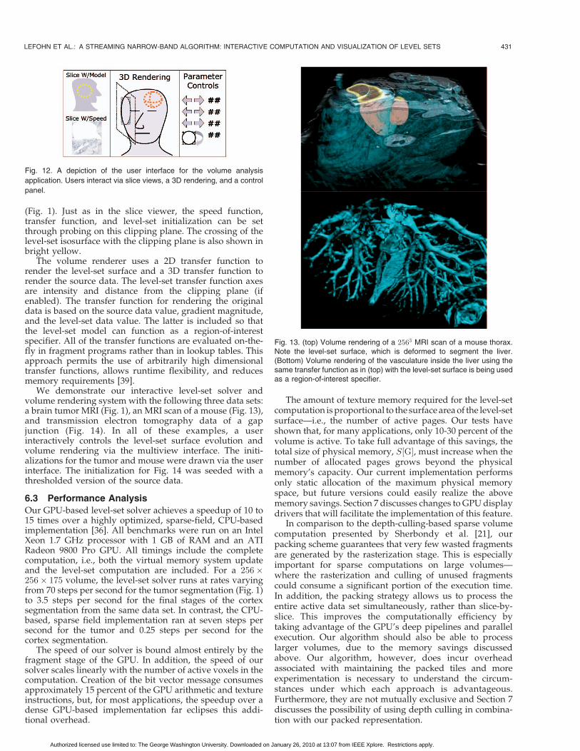
We demonstrate our interactive level-set solver andvolume rendering system with the following three data sets:a brain tumor MRI (Fig. 1), an MRI scan of a mouse (Fig. 13),and transmission electron tomography data of a gapjunction (Fig. 14). In all of these examples, a userinteractively controls the level-set surface evolution andvolume rendering via the multiview interface. The initi-alizations for the tumor and mouse were drawn via the userinterface. The initialization for Fig. 14 was seeded with athresholded version of the source data.

6.3 Performance Analysis

Our GPU-based level-set solver achieves a speedup of 10 to15 times over a highly optimized, sparse-field, CPU-basedimplementation [36]. All benchmarks were run on an IntelXeon 1.7 GHz processor with 1 GB of RAM and an ATIRadeon 9800 Pro GPU. All timings include the completecomputation, i.e., both the virtual memory system updateand the level-set computation are included. For a 256�256� 175 volume, the level-set solver runs at rates varyingfrom 70 steps per second for the tumor segmentation (Fig. 1)to 3.5 steps per second for the final stages of the cortexsegmentation from the same data set. In contrast, the CPU-based, sparse field implementation ran at seven steps persecond for the tumor and 0.25 steps per second for thecortex segmentation.

The speed of our solver is bound almost entirely by thefragment stage of the GPU. In addition, the speed of oursolver scales linearly with the number of active voxels in thecomputation. Creation of the bit vector message consumesapproximately 15 percent of the GPU arithmetic and textureinstructions, but, for most applications, the speedup over adense GPU-based implementation far eclipses this addi-tional overhead.

The amount of texture memory required for the level-setcomputation isproportional to the surface areaof the level-setsurface—i.e., the number of active pages. Our tests haveshown that, for many applications, only 10-30 percent of thevolume is active. To take full advantage of this savings, thetotal size of physical memory, S½G�, must increase when thenumber of allocated pages grows beyond the physicalmemory’s capacity. Our current implementation performsonly static allocation of the maximum physical memoryspace, but future versions could easily realize the abovememory savings. Section 7 discusses changes to GPUdisplaydrivers that will facilitate the implementation of this feature.

In comparison to the depth-culling-based sparse volumecomputation presented by Sherbondy et al. [21], ourpacking scheme guarantees that very few wasted fragmentsare generated by the rasterization stage. This is especiallyimportant for sparse computations on large volumes—where the rasterization and culling of unused fragmentscould consume a significant portion of the execution time.In addition, the packing strategy allows us to process theentire active data set simultaneously, rather than slice-by-slice. This improves the computationally efficiency bytaking advantage of the GPU’s deep pipelines and parallelexecution. Our algorithm should also be able to processlarger volumes, due to the memory savings discussedabove. Our algorithm, however, does incur overheadassociated with maintaining the packed tiles and moreexperimentation is necessary to understand the circum-stances under which each approach is advantageous.Furthermore, they are not mutually exclusive and Section 7discusses the possibility of using depth culling in combina-tion with our packed representation.


Fig. 12. A depiction of the user interface for the volume analysis

application. Users interact via slice views, a 3D rendering, and a control

panel.

Fig. 13. (top) Volume rendering of a 2563 MRI scan of a mouse thorax.Note the level-set surface, which is deformed to segment the liver.(Bottom) Volume rendering of the vasculature inside the liver using thesame transfer function as in (top) with the level-set surface is being usedas a region-of-interest specifier.


As with any sparse algorithm, it will be advantageous tosimply compute the entire (original) domain if the activedomain becomes sufficiently large. Our experience withsegmentation thus far, however, has shown that the thecomputation remains sufficiently sparse even for largestructures such as a cerebral cortex segmentation. Thesparseness is due to the fact that only the surface needs torepresented and the interior regions need not be repre-sented or computed.

7 CONCLUSIONS AND FUTURE WORK

This paper demonstrates a new tool for interactive volumeexploration and analysis that combines the quantitativecapabilities of deformable isosurfaces with the qualitativepower of volume rendering. By relying on graphicshardware, the level-set solver operates at interactive rates(approximately 15 times faster than previous solutions).This mapping relies on an efficient multidimensionalvirtual memory system to implement a time-dependent,sparse computation scheme. The memory mappings areupdated via a novel GPU-to-CPU message passing algo-rithm. The GPU renders the level-set surface model directlyfrom a sparse, compressed texture format. Future exten-sions and applications of the level-set solver include theprocessing of multivariate data as well as surface recon-struction and surface processing. Most of these only involvechanging only the speed functions.

There are a couple of ways in which the memory andcomputational efficiency of our solver can be improved.First, it may be worth achieving an even narrower band ofcomputation around the level-set model. This is possible byusing depth culling to avoid computation on inactiveelements within each active page [21]. Implementing thisdepth culling requires a memory model in which anarbitrary number of data buffers can access a single depthbuffer. The second optimization is to allow the total amountof physical memory to change at runtime and grow to thelimits of GPU memory. This requires spreading physicalmemory across multiple 2D textures (i.e., creating a3D physical memory space). The proposed super buffer [40]OpenGL extension supports both of these proposedoptimizations.

The GPU virtual memory abstraction also indicatespromising future research. We are currently beginningwork on a more general virtual memory implementationthat fully abstracts N-dimensional GPU memory. The goalis to provide an API that allows a GPU applicationprogrammer to specify an optimal physical and virtualmemory layout for their problem, then write the computa-tional kernels irrespective of the physical layout. Thekernels will specify memory accesses via abstract memoryaccess interfaces and an operating-system-like layer willreplace these memory access calls with the appropriateaddress translation code.

ACKNOWLEDGMENTS

Thanks to Evan Hart, Mark Segal, Jeff Royal and JasonMitchell at ATI for donating technical advice and hardwareto this project. Gordon Kindlmann’s nrrd toolkit was usedfor data set manipulation (http://teem.sourceforge.net).Milan Ikits’ GLEW library was used for OpenGL extensionmanagement (http://glew.sourceforge.net). Steve Lamontand Gina Sosinsky at the National Center for Microscopyand Imaging Research at the University of California at SanDiego provided the tomography data. Simon Warfield,Michael Kaus, Ron Kikinis, Peter Black, and Ferenc Joleszprovided the MRI head data. The mouse data was suppliedby the Center for In Vivo Microscopy at Duke University.This work was supported by grants ACI0089915 andCCR0092065 from the US National Scienc Foundation andUS Office of Naval Research N000140110033. The authorsalso thank John Owens and the anonymous reviewers fortheir input on the manuscript.

REFERENCES

[1] S. Osher and J. Sethian, “Fronts Propagating with Curvature-Dependent Speed: Algorithms Based on Hamilton-Jacobi For-mulations,” J. Computational Physics, vol. 79, pp. 12-49, 1988.

[2] R. Fedkiw and S. Osher, Level Set Methods and Dynamic ImplicitSurfaces. Springer, 2002.

[3] J.A. Sethian, Level Set Methods and Fast Marching Methods EvolvingInterfaces in Computational Geometry, Fluid Mechanics, ComputerVision, and Materials Science. Cambridge Univ. Press, 1999.

[4] R.T. Whitaker, “Volumetric Deformable Models: Active Blobs,”Proc. Visualization in Biomedical Computing 1994, R.A. Robb, ed.,pp. 122-134, 1994.

[5] T. Tasdizen, R. Whitaker, P. Burchard, and S. Osher, “GeometricSurface Smoothing via Anisotropic Diffusion of Normals,” Proc.IEEE Visualization, pp. 125-132, Oct. 2002.

[6] R. Whitaker, “A Level-Set Approach to 3D Reconstruction fromRange Data,” Int’l J. Computer Vision, pp. 203-231, Oct. 1998

[7] T. Yoo, U. Neumann, H. Fuchs, S. Pizer, T. Cullip, J. Rhoades, andR. Whitaker, “Direct Visualization of Volume Data,” IEEEComputer Graphics and Applications, vol. 12, pp. 63-71, 1992.

[8] M. Droske, B. Meyer, M. Rumpf, and C. Schaller, “An AdaptiveLevel Set Method for Medical Image Segmentation,” Proc. Ann.Symp. Information Processing in Medical Imaging, R. Leahy andM. Insana, eds. 2001.

[9] D. Adalsteinson and J.A. Sethian, “A Fast Level Set Method forPropogating Interfaces,” J. Computational Physics, pp. 269-277,1995.

[10] D. Peng, B. Merriman, S. Osher, H. Zhao, and M. Kang, “A PDEBased Fast Local Level Set Method,” J. Computational Physics,vol. 155, pp. 410-438, 1999.

[11] J. Owens, “Computer Graphics on a Stream Architecture,” PhDthesis, Stanford Univ., Nov. 2002.

[12] N. Goodnight, C. Woolley, G. Lewin, D. Luebke, and G.Humphreys, “A Multigrid Solver for Boundary Value ProblemsUsing Programmable Graphics Hardware,” Proc. Graphics Hard-ware 2003, pp. 102-111, July 2003.


Fig. 14. Segmentation and volume rendering of 512� 512� 61 3Dtransmission electron tomography data. The picture shows cytoskeletalmembrane extensions and connexins (pink surfaces extracted with thelevel-set models) near the gap junction between two cells (volumerendered in cyan).


[13] E.S. Larsen and D. McAllister, “Fast Matrix Multiplies UsingGraphics Hardware,” Proc. Super Computing 2001, Nov. 2001.

[14] R. Strzodka and M. Rumpf, “Using Graphics Cards for QuantizedFEM Computations,” Proc. VIIP Conf. Visualization and ImageProcessing, 2001.

[15] M. Rumpf and R. Strzodka, “Level Set Segmentation in GraphicsHardware,” Proc. Int’l Conf. Image Processing, pp. 1103-1106, 2001.

[16] A.E. Lefohn and R.T. Whitaker, “A GPU-Based, Three-Dimen-sional Level Set Solver with Curvature Flow,” Tech Report UUCS-02-017, Univ. of Utah, Dec. 2002.

[17] J. Bolz, I. Farmer, E. Grinspun, and P. Schroder, “Sparse MatrixSolvers on the GPU: Conjugate Gradients and Multigrid,” ACMTrans. Graphics, vol. 22, pp. 917-924, July 2003.

[18] J. Kruger and R. Westermann, “Linear Algebra Operators for GPUImplementation of Numerical Algorithms,” ACM Trans. Graphics,vol. 22, pp. 908-916, July 2003.

[19] A.C. Beers, M. Agrawala, and N. Chaddha, “Rendering fromCompressed Textures,” Proc. SIGGRAPH ’96, Computer GraphicsProc., Ann. Conf. Series, pp. 373-378, Aug. 1996.

[20] M. Kraus and T. Ertl, “Adaptive Texture Maps,” Proc. GraphicsHardware 2002, pp. 7-16, Sept. 2002.

[21] A. Sherbondy, M. Houston, and S. Nepal, “Fast VolumeSegmentation with Simultaneous Visualization Using Program-mable Graphics Hardware,” Proc. IEEE Visualization, pp. 171-176,Oct. 2003.

[22] R.A. Drebin, L. Carpenter, and P. Hanrahan, “Volume Render-ing,” Computer Graphics (Proc. SIGGRAPH ’88), vol. 22, pp. 65-74,Aug. 1988.

[23] M. Levoy, “Display of Surfaces from Volume Data,” IEEEComputer Graphics and Applications, vol. 8, pp. 29-37, 1988.

[24] P. Sabella, “A Rendering Algorithm for Visualizing 3D ScalarFields,” Computer Graphics (Proc. SIGGRAPH ’88), vol. 22, pp. 51-58, Aug. 1988.

[25] B. Cabral, N. Cam, and J. Foran, “Accelerated Volume Renderingand Tomographic Reconstruction Using Texture Mapping Hard-ware,” Proc. ACM Symp. Volume Visualization, pp. 91-98, Oct. 1994.

[26] O. Wilson, A.V. Gelder, and J. Wilhelms, “Direct VolumeRendering via 3D Textures,” Technical Report UCSC-CRL-94-19,Univ. of California at Santa Cruz, June 1994.

[27] K. Engel, M. Kraus, and T. Ertl, “High-Quality Pre-IntegratedVolume Rendering Using Hardware-Accelerated Pixel Shading,”Proc. Graphics Hardware 2001, 2001.

[28] J. Kniss, G. Kindlmann, and C. Hansen, “Multi-DimensionalTransfer Functions for Interactive Volume Rendering,” IEEETrans. Visualization and Computer Graphics, vol. 8, no. 3, pp. 270-285, July-Sept. 2002.

[29] T.J. Purcell, I. Buck, W.R. Mark, and P. Hanrahan, “Ray Tracing onProgrammable Graphics Hardware,” ACM Trans. Graphics, vol. 21,pp. 703-712, July 2002.

[30] A. Silberschatz and P. Galvin, Operating System Concepts. Addison-Wesley, 1998.

[31] U. Kapasi, W. Dally, S. Rixner, P. Mattson, J. Owens, and B.Khailany, “Efficient Conditional Operations for Data-ParallelArchitectures,” Proc. 33rd Ann. Int’l Symp. Microarchitecture,pp. 159-170, 2000.

[32] A.E. Lefohn, J. Kniss, C. Hansen, and R. Whitaker, “InteractiveDeformation and Visualization of Level Set Surfaces UsingGraphics Hardware,” Proc. IEEE Visualization, pp. 75-82, Oct. 2003.

[33] A.E. Lefohn, J. Kniss, C. Hansen, and R. Whitaker, “A StreamingNarrow-Band Algorithm: Supplemental Information,” http://computer.org/tvcg/archives.htm, 2004.

[34] R. Fedkiw, T. Aslam, B. Merriman, and S. Osher, “A Non-Oscillatory Eulerian Approach to Interfaces in MultimaterialFlows (the Ghost Fluid Method),” J. Computational Physics,vol. 152, pp. 457-492, 1999.

[35] J. Kniss, S. Premoze, C. Hansen, P. Shirley, and A. McPherson, “AModel for Volume Lighting and Modeling,” IEEE Trans. Visualiza-tion and Computer Graphics, vol. 9, no. 2, pp. 150-162, Apr.-June2003.

[36] “The Insight Toolkit,” http://www.itk.org, 2003.[37] R. Malladi, J.A. Sethian, and B.C. Vemuri, “Shape Modeling with

Front Propagation: A Level Set Approach,” IEEE Trans. PatternAnalysis and Machine Intelligence, vol. 17, pp. 158-175, 1995.

[38] A.E. Lefohn, J. Cates, and R. Whitaker, “Interactive, GPU-BasedLevel Sets for 3D Brain Tumor Segmentation,” Medical ImageComputing and Computer Assisted Intervention, pp. 564-572, 2003.

[39] J. Kniss, S. Premoze, M. Ikits, A.E. Lefohn, and C. Hansen,“Gaussian Transfer Functions for Multi-Field Volume Visualiza-tion,” Proc. IEEE Visualization, pp. 497-504, Oct. 2003.

[40] J. Percy and R. Mace, “OpenGL Extensions: Siggraph 2003,”http://mirror.ati.com/developer/techpapers.html, 2003.

[41] R. Whitaker and X. Xue, “Variable-Conductance, Level-SetCurvature for Image Denoising,” Proc. IEEE Int’l Conf. ImageProcessing, pp. 142-145, Oct. 2001.

Aaron E. Lefohn is a PhD student in theComputer Science Department at the Universityof California at Davis and a graphics softwareengineer at Pixar Animation Studios. He re-ceived the MS degree in computer science fromthe University of Utah in 2003, the MS degree intheoretical chemistry from the University of Utahin 2001, and the BA degree in chemistry fromWhitman College in 1997. His research interestsinclude general computation with graphics hard-

ware, physically-based animation, and photorealistic rendering. He is aUS National Science Foundation graduate fellow in computer scienceand a student member of the IEEE.

Joe M. Kniss is a PhD student at the Universityof Utah and a member of the Scientific Comput-ing and Imaging Institute. He received the BSdegree in computer science from Idaho StateUniversity in 1999 and the MS degree incomputer science from the University of Utahin 2002. He has conducted research in volumerendering, light transport, human computerinteraction, and data classification. He is arecipient of the US Department of Energy’s High

Performance Computer Science (HPCS) graduate fellowship and is astudent member of the IEEE.

Charles D. Hansen received the BS degree incomputer science from Memphis State Univer-sity in 1981 and the PhD degree in computerscience from the University of Utah in 1987. Heis an associate professor of computer science atthe University of Utah. From 1997 to 1999, hewas a research associate professor in computerscience at Utah. From 1989 to 1997, he was atechnical staff member in the Advanced Com-puting Laboratory (ACL) located at Los Alamos

National Laboratory, where he formed and directed the visualizationefforts in the ACL. He was a Bourse de Chateaubriand PostDoc Fellowat INRIA, Rocquencourt, France, in 1987 and 1988. His researchinterests include large-scale scientific visualization and computergraphics. He is a member of the IEEE.

Ross T. Whitaker received the BS degree inelectrical engineering and computer sciencefrom Princeton University in 1986 summa cumlaude. From 1986 to 1988, he worked for theBoston Consulting Group, entering the Univer-sity of North Carolina at Chapel Hill (UNC) in1989. At UNC, he received the Alumni Scholar-ship Award, and received the PhD degree incomputer science in 1994. From 1994-1996, heworked at the European Computer-Industry

Research Centre in Munich, Germany, as a research scientist in theUser Interaction and Visualization Group. From 1996-2000, he was anassistant professor in the Department of Electrical Engineering at theUniversity of Tennessee. Since 2000, he has been at the University ofUtah, where he is an associate professor in the College of Computingand a faculty member of the Scientific Computing and Imaging Institute.He is a member of the IEEE.

. For more information on this or any computing topic, please visitour Digital Library at www.computer.org/publications/dlib.



Documents

422 IEEE TRANSACTIONS ON VISUALIZATION AND COMPUTER