IEEE TRANSACTIONS ON VISUALIZATION AND COMPUTER GRAPHICS …graphics.stanford.edu/~pmerrell/tvcg.pdf · IEEE TRANSACTIONS ON VISUALIZATION AND COMPUTER GRAPHICS 1 ... A General Procedural

IEEE TRANSACTIONS ON VISUALIZATION AND COMPUTER GRAPHICS 1

Model Synthesis: A General ProceduralModeling Algorithm

Paul Merrell and Dinesh ManochaUniversity of North Carolina at Chapel Hill

Abstract—We present a method for procedurally modeling general complex 3D shapes. Our approach can automatically generatecomplex models of buildings, man-made structures, or urban datasets in a few minutes based on user-defined inputs. The algorithmattempts to generate complex 3D models that resemble a user-defined input model and that satisfy various dimensional, geometric,and algebraic constraints to control the shape. These constraints are used to capture the intent of the user and generate shapes thatlook more natural. We also describe efficient techniques to handle complex shapes, highlight its performance on many different typesof models. We compare model synthesis algorithms with other procedural modeling techniques, discuss the advantages of differentapproaches, and describe as close connection between model synthesis and context-sensitive grammars.

Index Terms—model synthesis, procedural modeling

F

1 INTRODUCTION

C REATING 3D digital content for computer games,movies, and virtual environments is an important

and challenging problem. It is difficult because objectsin the real-world are complex and have widely varyingshapes and styles. Consider the problem of generatinga realistic 3D model of an outdoor scene. Differentapplications may require many different types of modelssuch as buildings, oil platforms, spacecrafts, roller coast-ers, and other man-made structures. Overall, geometricmodeling is a creative and artistic process. However,current modeling systems can be cumbersome and theusers often spend a lot of time performing routine andtedious tasks instead of making creative decisions.

Despite extensive work in geometric modeling forover four decades, it remains a time-consuming task.Learning how to use current geometric modeling toolscan require significant training and even when the toolsare mastered creating complex models is still difficult.With state of the art 3D CAD and modeling tools, theuser can create simple geometric primitives and modifythem using various transformations and geometric op-erations. Modeling complex environments such as citiesor a landscapes requires the creation and manipulationof large numbers of primitives and can take many hoursor days [31].

Many objects and environments contain repetitive andself-similar structures which can be modeled more eas-ily using procedural modeling techniques. Proceduralmodeling techniques are designed to automatically orsemi-automatically generate complex models. These in-clude techniques based on shape grammars, scriptinglanguages, L-systems, fractals, solid texturing, etc. Theseapproaches have been used to generate many complexshapes, but each method is mainly limited to a specificclass of models or requires considerable user input or

guidance.In this paper, we address the problem of generating

complex models using model synthesis. Model synthesisis a simple technique [26], [28] proposed to automaticallygenerate complex shapes. The model synthesis algorithmaccepts a simple 3D shape as an input and then gener-ates a larger and more complex model that resemblesthe input in terms of its shape and local features. Anexample of this is shown in Figure 1.

Different procedural modeling techniques requirevarying degrees of user input. Using a high degreeof user input has both advantages and disadvantages.Without sufficient user input, the result generated by aprocedural modeling method may be too random andsome parts of the generated 3D model may turn out to bedifferent from the user’s original intent. With too muchuser input, the time required to adjust and manipulatethe model could overwhelm the user. Ideally, the usercould choose to provide any amount of input and thealgorithm should be able to adjust accordingly. The userinput can often be specified in the form of a set ofconstraints on the output. Any output that satisfies all ofthe user’s constraint is acceptable. Prior work in modelsynthesis [28] uses a minimal amount of user input inthe form of a single adjacency constraint and may notgive the user enough control over the result.

We present a novel model synthesis algorithm whichenables the user to specify geometric constraints thatgive the user greater control over the results. We usedimensional, incident, algebraic, and connectivity con-straints that have been used in CAD/CAM, geometricmodeling, and robotics. The constraints are specified be-tween a set of geometric objects and their features. Theseinclude spatial and logical constraints such as incidence,tangency, perpendicularity, and metric constraints suchas distance, angle, etc. We use these constraints to cap-ture the user’s intent, to prevent objects from becoming


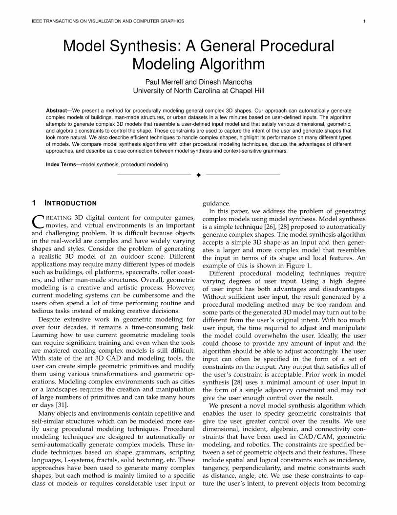
(a) Example Model (b) Generated Model

Fig. 1. (a) From an example model specified by the user, (b) a model of several oil platforms is generated automaticallyby our algorithm. The shape of the output resembles the input and fits several dimensional and connectivity constraints.The height of the platform and the length and width of the beams are constrained to have a particular size. The shapesare constrained to be in four connected groups. Our algorithm can generate the new model in about half a minute.

unnaturally large or small, to generate more complexshapes, and to manage the objects’ spatial distribution.

In order to satisfy the constraints, we represent localneighborhoods of the objects using Boolean expressions.The Boolean expressions are used to compute how dif-ferent vertices, edges and faces of the synthesized modelconnect together. Furthermore, we present a scheme toincorporate dimensional and algebraic constraints intoour model synthesis algorithm.

Like most procedural modeling techniques, our al-gorithm is primarily designed to work on objects thatare self-similar. We demonstrate its ability to generatemodels of buildings, man-made structures, city streets,plumbling, etc.

A preliminary version of this paper appeared in [29].We also compare model synthesis to other proceduralmodeling techniques which are often based on usinggrammars. We show that model synthesis is particularlyuseful for generating architectural shapes, but has dif-ficulty with some curved and organic shapes. We alsoestablish a close relationship between contex-sensitivegrammars and model synthesis by showing that a prob-lem in one domain can be reduced to a problem in theother domain.

The rest of the paper is organized as follows. We givea brief survey of prior work on procedural modeling andgeometric constraint systems in Section 2. Section 3 givesa brief overview of model synthesis and the constraintsused by our algorithm. The overall constraint-basedalgorithm is described in Section 4 and we highlight itsperformance in Section 5. We analyze its performanceand discuss its limitations in Section 6. We compare it torelated work on procedural modeling in Section 7.

2 RELATED WORK

In this section, we briefly survey related work on proce-dural modeling, texture synthesis, and model synthesis.

2.1 Procedural Modeling

Many procedural modeling techniques have been de-veloped over the last few decades. These techniquesare very diverse, but most of them are targeted to-wards modeling a specific type of object or environment.Techniques based on fractal geometry achieved successmodeling natural landscapes [13], [23], [32].

There is a long history of modeling plants procedu-rally. Many plant modeling techniques use a formalgrammar call an L-system. L-systems were proposedby Lindenmayer as a general framework for describingplant growth and plant models [22], [36]. An L-systemis a parallel rewriting system. L-systems can be extendedto consider how plants interact with their environmentas they grow [25]. Other techniques use sketches [8],photographs [38] or positional information [37] toinfluence the shape of the plant models.

Many procedural techniques are designed specificallyfor modeling urban models [45], [43]. Like many plantmodeling techniques, some urban modeling techniquesuse L-systems. L-systems have been used to generateroad networks and buildings on land between the roads[34]. Other grammars have been introduced specificallyfor modeling architecture. Shape grammars were intro-duced as a tool for analyzing and designing architecture[40], [12]. Wonka et al. introduced a related group ofgrammars called split grammars [49]. Split grammarsoperate by splitting shapes into smaller components and


can generate highly detailed models of architecture. Splitgrammars were further developed by Muller et al. [31].They developed shape operations for mass modelingand for aligning many parts of a building’s designtogether.

Some techniques focus more on the 2D layouts of citiesthan on the 3D shapes of the buildings. Chen et al. [7]allow the users to edit a city’s street layout interactivelyusing tensor fields. Aliaga et al. [2] generate street lay-outs using an example-based method. A related area ofresearch is urban simulation which seeks to understandhow various factors influence a cities development andgrowth over time [41], [44]. Aspects of urban simulationhave been used in procedural modeling to produce morerealistic models of cities [46].

Other techniques are designed to model smaller struc-tures. Legakis et al. [21] propose a method for auto-matically embellishing 3D surfaces with various cellulartextures including bricks, stones and tiles. Cutler et al.[9] developed a method for modeling layered, solidmodels with an internal structure. Another method hasbeen developed to model truss structures by optimizingthe locations and strengths of beams and joints [39].Pottmann et al. [35] have developed algorithms basedon Discrete Differential Geometry that determine howto arrange beams and glass panels so they form in theshape of a given freeform surface and satisfy variousgeometric and physical constraints.

Another way to model objects is to combine to-gether parts of existing models interactively [14]. In thismethod, the user can search through a large databaseof 3D models to find a desired part, then cut the partout from the model, and stitch various parts together tocreate a new object.

2.2 Modeling with ConstraintsThere is rich literature in solid modeling on designingshapes that satisfy various geometric, parametric orvariational constraints [6], [1]. There is also considerablework on solving geometric constrained systems andsome excellent surveys are available [16], [18]. Geometricconstraints are widely used in computer aided engineer-ing applications [15] and also arise in many geometricmodeling contexts such as virtual reality, robotics, molec-ular modeling, computer vision, etc. These constraintsare used to incorporate relationships between geometricentities and features and thereby capture the intent ofthe designers. Our formulation of various constraints issimilar, though our approach to satisfy these constraintsduring model synthesis is different. Besides geometricconstraints, silhouette-based constraints are also usedto model freeform objects using sketch-based interfaces[17], [33].

2.3 Texture Synthesis and Model SynthesisThe model synthesis algorithm itself has much in com-mon with texture synthesis. The field of texture synthesis

has seen a proliferation of new algorithms and new ideasover the past decade. This section gives an overviewof the most relevant developments and explains theirrelationship to model synthesis. A more comprehensivesurvey is given in [47].

Many texture synthesis algorithms were influenced bya seminal paper written by Efros and Leung [11]. Theiralgorithm is remarkably simple. It generates textures byadding pixels individually by finding a neighborhoodthat matches the neighborhood around the insertionpoint. There are several ways to accelerate texture syn-thesis such as by adding the pixels in a particular order[48], by adding patches of texture rather than individualpixels [10], [20], or by exploiting spatial coherence [3].

Texture synthesis has also been used to generate tex-ture maps directly onto curved surfaces [42]. Texturesynthesis has been extended into three dimensions isto create solid textures [19]. Texture synthesis has alsobeen used to generate geometric textures [4], [51] whichcombine elements of texture mapping and modeling.They are used like texture maps to apply patterns toobjects, but the patterns change the shape of the objectto create effects like bumps or dimples or chain mail.

Texture synthesis was the inspiration behind modelsynthesis. Model synthesis was initially proposed byMerrell [26] and later extended to handle non-axis-aligned objects [28]. Both model and texture synthesis aredesigned to take a small sample as an input example andgenerate a larger result that resembles the input example.

Model synthesis relies on finding symmetric patterns.Many methods have been developed to find patterns in3D models [24]. Bokeloh et al. [5] automatically identifysymmetries within objects and use these symmetries tocut objects into pieces. By editing these pieces, a shapegrammar is derived.

3 ALGORITHM

In this section, we give a brief overview of modelsynthesis and the constraints used in the algorithm.

3.1 Notation

Points and vectors are written in bold face, x ∈ R3.Lower-case letters not in bold face are generally used todenote scalar variables, but there are a few exceptions.The variable h is used to denote the set of points withina half-space. The upper-case letters, E and M are usedto denote the models. The model E is the input examplemodel provided by the user. The model M is the newmodel generated by the algorithm. Each model is a setof closed polyhedra. The models E and M and thehalf-spaces hi are represented in two different ways. Ahalf-space h1 could be represented as a set of pointsh1 or as the characteristic function of that set h1(x)where h1(x) = 1 if x ∈ h1, otherwise h1(x) = 0. Thecomplement of the half-space h1 is written as either theset hC1 or the function ¬h1(x).


3.2 Background

Our algorithm builds upon earlier work in model syn-thesis. In this section, we give a brief overview of a previ-ous model synthesis algorithm [28]. The user provides anexample model as the input. The example model is a setof polygons that form closed polyhedral objects. Modelsynthesis generates a new model M that resembles theexample model E. In earlier work, it was assumed thatthe input was a single object, but we allow multipleobjects in E. Let n be the number of different objectsin E. We consider the example model to be a functionE(x) of a point in space x where E(x) = k if x is insidean object of type k where 1 ≤ k ≤ n. If x is not insideany of the objects, then E(x) = 0. The function M(x) issimilarly defined for the new model M .

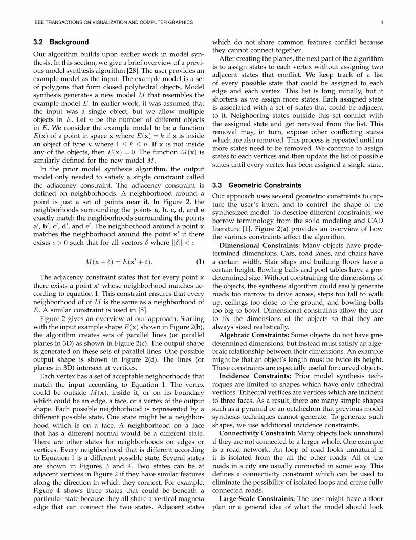
In the prior model synthesis algorithm, the outputmodel only needed to satisfy a single constraint calledthe adjacency constraint. The adjacency constraint isdefined on neighborhoods. A neighborhood around apoint is just a set of points near it. In Figure 2, theneighborhoods surrounding the points a, b, c, d, and eexactly match the neighborhoods surrounding the pointsa′, b′, c′, d′, and e′. The neighborhood around a point xmatches the neighborhood around the point x′ if thereexists ε > 0 such that for all vectors δ where ||δ|| < ε

M(x+ δ) = E(x′ + δ). (1)

The adjacency constraint states that for every point xthere exists a point x′ whose neighborhood matches ac-cording to equation 1. This constraint ensures that everyneighborhood of of M is the same as a neighborhood ofE. A similar constraint is used in [5].

Figure 2 gives an overview of our approach. Startingwith the input example shape E(x) shown in Figure 2(b),the algorithm creates sets of parallel lines (or parallelplanes in 3D) as shown in Figure 2(c). The output shapeis generated on these sets of parallel lines. One possibleoutput shape is shown in Figure 2(d). The lines (orplanes in 3D) intersect at vertices.

Each vertex has a set of acceptable neighborhoods thatmatch the input according to Equation 1. The vertexcould be outside M(x), inside it, or on its boundarywhich could be an edge, a face, or a vertex of the outputshape. Each possible neighborhood is represented by adifferent possible state. One state might be a neighbor-hood which is on a face. A neighborhood on a facethat has a different normal would be a different state.There are other states for neighborhoods on edges orvertices. Every neighborhood that is different accordingto Equation 1 is a different possible state. Several statesare shown in Figures 3 and 4. Two states can be atadjacent vertices in Figure 2 if they have similar featuresalong the direction in which they connect. For example,Figure 4 shows three states that could be beneath aparticular state because they all share a vertical magnetaedge that can connect the two states. Adjacent states

which do not share common features conflict becausethey cannot connect together.

After creating the planes, the next part of the algorithmis to assign states to each vertex without assigning twoadjacent states that conflict. We keep track of a listof every possible state that could be assigned to eachedge and each vertex. This list is long initially, but itshortens as we assign more states. Each assigned stateis associated with a set of states that could be adjacentto it. Neighboring states outside this set conflict withthe assigned state and get removed from the list. Thisremoval may, in turn, expose other conflicting stateswhich are also removed. This process is repeated until nomore states need to be removed. We continue to assignstates to each vertices and then update the list of possiblestates until every vertex has been assigned a single state.

3.3 Geometric Constraints

Our approach uses several geometric constraints to cap-ture the user’s intent and to control the shape of thesynthesized model. To describe different constraints, weborrow terminology from the solid modeling and CADliterature [1]. Figure 2(a) provides an overview of howthe various constraints affect the algorithm.

Dimensional Constraints: Many objects have prede-termined dimensions. Cars, road lanes, and chairs havea certain width. Stair steps and building floors have acertain height. Bowling balls and pool tables have a pre-determined size. Without constraining the dimensions ofthe objects, the synthesis algorithm could easily generateroads too narrow to drive across, steps too tall to walkup, ceilings too close to the ground, and bowling ballstoo big to bowl. Dimensional constraints allow the userto fix the dimensions of the objects so that they arealways sized realistically.

Algebraic Constraints: Some objects do not have pre-determined dimensions, but instead must satisfy an alge-braic relationship between their dimensions. An examplemight be that an object’s length must be twice its height.These constraints are especially useful for curved objects.

Incidence Constraints: Prior model synthesis tech-niques are limited to shapes which have only trihedralvertices. Trihedral vertices are vertices which are incidentto three faces. As a result, there are many simple shapessuch as a pyramid or an octahedron that previous modelsynthesis techniques cannot generate. To generate suchshapes, we use additional incidence constraints.

Connectivity Constraint: Many objects look unnaturalif they are not connected to a larger whole. One exampleis a road network. An loop of road looks unnatural ifit is isolated from the all the other roads. All of theroads in a city are usually connected in some way. Thisdefines a connectivity constraint which can be used toeliminate the possibility of isolated loops and create fullyconnected roads.

Large-Scale Constraints: The user might have a floorplan or a general idea of what the model should look


(a) Flowchart (b) Example Shape E(x) (c) Parallel lines diving up theplane.

(d) Acceptable Output Shape M(x)

Fig. 2. (a) Overview flowchart showing how the constraints affect the algorithm. (b) From the input shape E, (c) setsof lines parallel to E intersect to form edges and vertices. (d) The output shape is formed within the parallel lines. Foreach selected point a, b, c, d, and e in M , there are points a′, b′, c′, d′, and e′ in the example model E which havethe same neighborhood. The models E and M contain two different kinds of object interiors shown in blue and brown.The brown object’s width is constrained to be one line spacing width. The width of the blue object is not constrained.The objects are also constrained to be fully connected.

like on a macroscopic scale. For example, the user mightwant to build a city with buildings arranged in the shapeof a circle or a triangle. The user can generate such amodel by using large-scale constraints. These constraintsare specified on a large volumetric grid where each voxelrecords which objects should appear within it.

4 CONSTRAINT-BASED APPROACH

In this section, we present our constraint-based synthesisalgorithm.

4.1 Overview

We first discuss incidence constraints that specify thatmore than three faces are incident to a vertex in or-der to generate non-trihedral vertices. To add incidenceconstraints, we need a new way to describe the neigh-borhoods around non-trihedral vertices. We use Booleanexpressions as explained in Section 4.2. These represen-tations are used to determine which neighborhoods canbe adjacent to one another. The vertices of the outputare constructed where several planes intersect. Verticesincident to four faces require that four planes intersectwhich requires the planes to be spaced a particular waydescribed in Section 4.4.

The Boolean expressions describing the states canalso be used to apply dimensional constraints to thesynthesized model. By disallowing any states that wouldpermit the objects to stretch beyond its fixed dimen-sions, dimensional constraints are created as describedin Section 4.5. Connectivity constraints are imposed inSection 4.6 by changing the order in which the states areassigned. Large-scale constraints are applied by chang-ing the probabilities of the states that are assigned toeach vertex, as described in Section 4.7. An algebraicconstraint is described in Section 4.8.

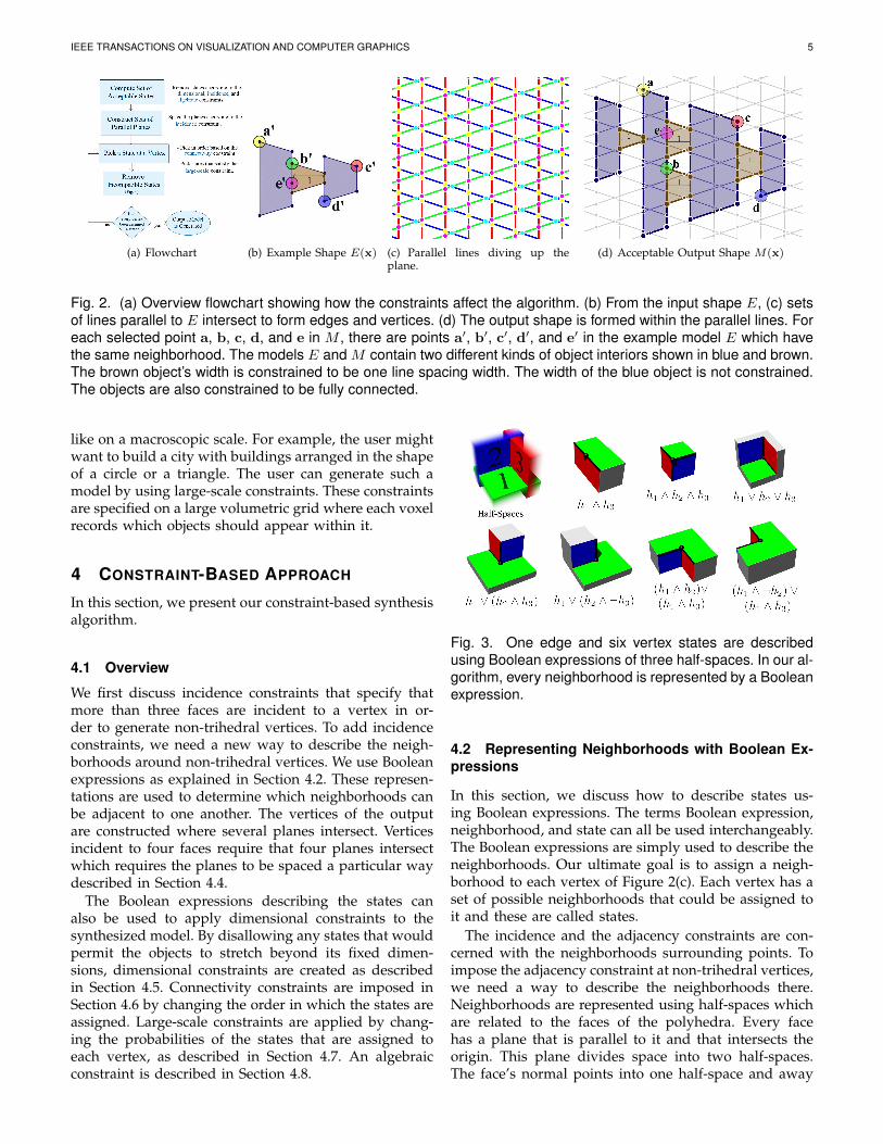
Fig. 3. One edge and six vertex states are describedusing Boolean expressions of three half-spaces. In our al-gorithm, every neighborhood is represented by a Booleanexpression.

4.2 Representing Neighborhoods with Boolean Ex-pressions

In this section, we discuss how to describe states us-ing Boolean expressions. The terms Boolean expression,neighborhood, and state can all be used interchangeably.The Boolean expressions are simply used to describe theneighborhoods. Our ultimate goal is to assign a neigh-borhood to each vertex of Figure 2(c). Each vertex has aset of possible neighborhoods that could be assigned toit and these are called states.

The incidence and the adjacency constraints are con-cerned with the neighborhoods surrounding points. Toimpose the adjacency constraint at non-trihedral vertices,we need a way to describe the neighborhoods there.Neighborhoods are represented using half-spaces whichare related to the faces of the polyhedra. Every facehas a plane that is parallel to it and that intersects theorigin. This plane divides space into two half-spaces.The face’s normal points into one half-space and away


from the other. Let us associate each face with the half-space that its normal points away from. These half-spaces can be used to describe every neighborhood of thepolyhedra using a combination of Boolean operations.A few examples of these combinations are shown inFigure 3. For every point p in E, there exists a Booleanexpression that will produce a neighborhood identicalto p. This set of Boolean operations is found using thefollowing method:

1) If p is on a face and hi is the half-space associatedwith the face, then hi alone produces a neighbor-hood that is identical to p. If p is on a face whosenormal points in the opposite direction, then hCidescribes the neighborhood around p.

2) If p is on an edge whose two adjacent faces areassociated with the two half-spaces hi and hj , thenthe neighborhood around p is described by hi ∪hjif the edge has a reflex angle and hi ∩ hj if it doesnot.

3) If p is on a vertex, then the procedure for comput-ing its neighborhood’s Boolean expression is morecomplex. Every face that intersects p is on a plane.Let us take all the faces that intersect p and useall of their planes to divide the space into cells. Anexample of this is shown in Figure 5. Each cell is theintersection of several half-spaces. Since the planesall intersect p, every cell has points in the neighbor-hood of p. For each cell, we determine if the pointswithin the cell and within the neighborhood of pare inside or outside the polyhedron E. We takethe union of all cells which have points inside thepolyhedron and this is the Boolean expression thatrepresents the neighborhood surrounding p. Eachcell is the intersection of several half-spaces and sothe neighborhood at p is represented as a unionof intersections. These expressions can often besimplified using familiar rules of Boolean algebrasuch as (hi∩hj)∪(hi∩hCj ) = hi. Simplified Booleanexpressions for various states are shown in Figures3 and 5.

This method gives us a Boolean expression describinghow a polyhedra intersects a neighborhood at any pointp. However, more than one polyhedra might intersectat the same point. For example, see the points b and eof Figure 2(d). When multiple objects intersect, we cancompute a Boolean expression for each object and thencombine all the expressions into one. Let k1 and k2 betwo object interiors and let b1 and b2 be two Booleanexpressions. The notation k1 · b1 + k2 · b2 will be used todescribe a neighborhood which contains the object k1 atthe points b1 and object k2 at b2. For example, 1·h1∩hC2 +3 · h2 describes a neighborhood where an edge h1 ∩ hC2of object 1 touches a face of h2 of object 3.

4.3 Evaluating Boolean Expressions along EdgesIn the previous section, we discuss how to describe everyneighborhood or every state as a Boolean expression, but

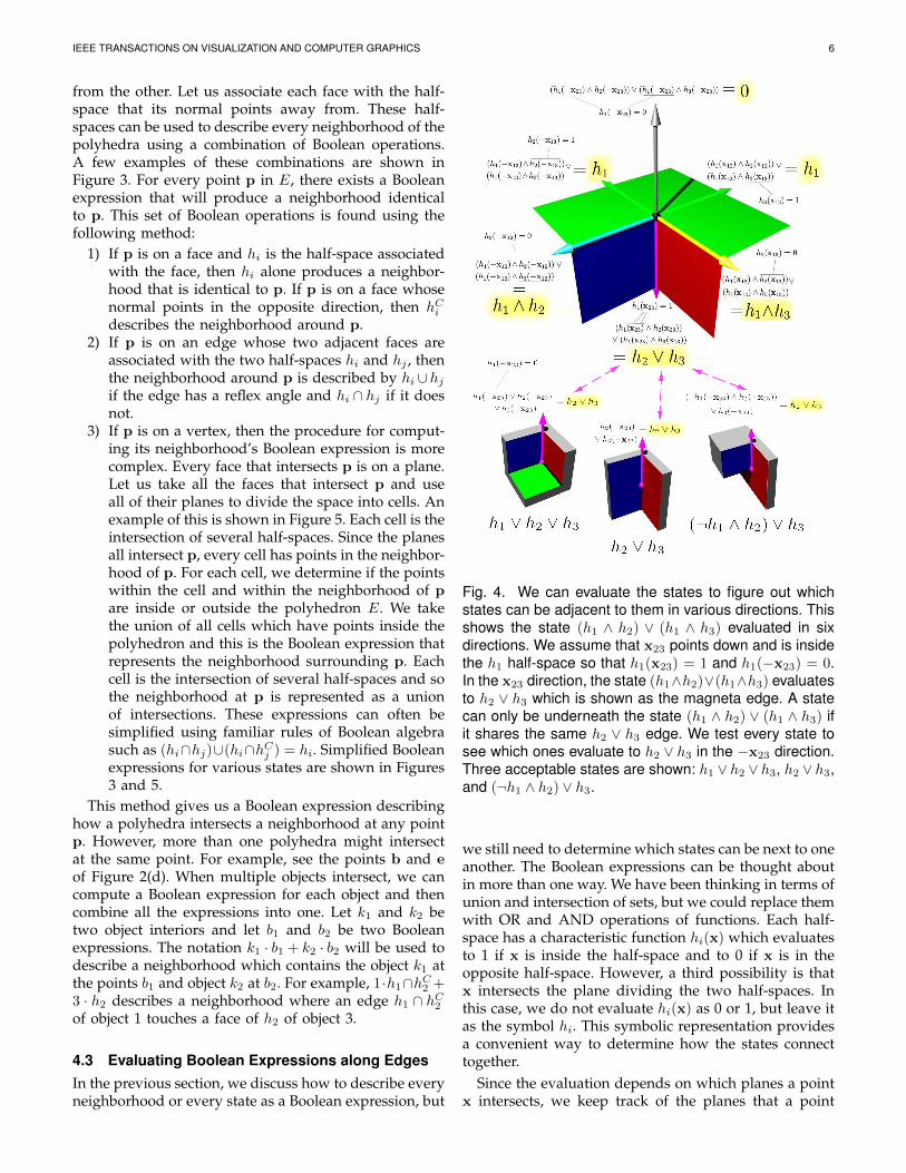
Fig. 4. We can evaluate the states to figure out whichstates can be adjacent to them in various directions. Thisshows the state (h1 ∧ h2) ∨ (h1 ∧ h3) evaluated in sixdirections. We assume that x23 points down and is insidethe h1 half-space so that h1(x23) = 1 and h1(−x23) = 0.In the x23 direction, the state (h1∧h2)∨(h1∧h3) evaluatesto h2 ∨ h3 which is shown as the magneta edge. A statecan only be underneath the state (h1 ∧ h2) ∨ (h1 ∧ h3) ifit shares the same h2 ∨ h3 edge. We test every state tosee which ones evaluate to h2 ∨ h3 in the −x23 direction.Three acceptable states are shown: h1 ∨ h2 ∨ h3, h2 ∨ h3,and (¬h1 ∧ h2) ∨ h3.

we still need to determine which states can be next to oneanother. The Boolean expressions can be thought aboutin more than one way. We have been thinking in terms ofunion and intersection of sets, but we could replace themwith OR and AND operations of functions. Each half-space has a characteristic function hi(x) which evaluatesto 1 if x is inside the half-space and to 0 if x is in theopposite half-space. However, a third possibility is thatx intersects the plane dividing the two half-spaces. Inthis case, we do not evaluate hi(x) as 0 or 1, but leave itas the symbol hi. This symbolic representation providesa convenient way to determine how the states connecttogether.

Since the evaluation depends on which planes a pointx intersects, we keep track of the planes that a point


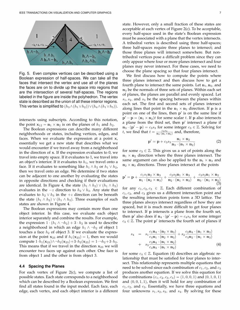
Fig. 5. Even complex vertices can be described using aBoolean expression of half-spaces. We can take all thefaces that intersect the vertex and use all of the planesthe faces are on to divide up the space into regions thatare the intersection of several half-spaces. The regionslabeled in the figure are inside the polyhedron. The vertexstate is described as the union of all these interior regions.This vertex is simplified to (h3∧(h1∨h2))∨(h4∧(h1∨h5)).

intersects using subscripts. According to this notation,the point x12 = n1 × n2 is on the planes of h1 and h2.

The Boolean expressions can describe many differentneighborhoods or states, including vertices, edges, andfaces. When we evaluate the expression at a point x,essentially we get a new state that describes what wewould encounter if we travel away from a neighborhoodin the direction of x. If the expression evaluates to 0, wetravel into empty space. If it evaluates to 1, we travel intoan object’s interior. If it evaluates to h1, we travel onto aface. If it evaluates to something like h1 ∧ h2 or h1 ∨ h2,then we travel onto an edge. We determine if two statescan be adjacent to one another by evaluating the statesin opposite directions and checking if their evaluationsare identical. In Figure 4, the state (h1 ∧ h2) ∨ (h1 ∧ h3)evaluates in the −z direction to h2 ∨ h3. Any state thatevaluates to h2 ∨ h3 in the +z direction can be beneaththe state (h1 ∧ h2) ∨ (h1 ∧ h3). Three examples of suchstates are shown in Figure 4.

The Boolean expressions may contain more than oneobject interior. In this case, we evaluate each objectinterior separately and combine the results. For example,the expression 1 · (h1 ∧ ¬h2) + 3 · h2 is used to describea neighborhood in which an edge h1 ∧ ¬h2 of object 1touches a face h2 of object 3. If we evaluate the expres-sion at the point x23 and if h1(x23) = 1, then we wouldcompute 1·h1(x23)∧¬h2(x23)+3·h2(x23) = 1·¬h2+3·h2.This means that if we travel in the direction x23 we willencounter two faces up against each other. One face isfrom object 1 and the other is from object 3.

4.4 Spacing the PlanesFor each vertex of Figure 2(c), we compute a list ofpossible states. Each state corresponds to a neighborhoodwhich can be described by a Boolean expression. We firstfind all states found in the input model. Each face, eachedge, each vertex, and each object interior is a different

state. However, only a small fraction of these states areacceptable at each vertex of Figure 2(c). To be acceptable,every half-space used in the state’s Boolean expressionmust be associated with a plane that the vertex intersects.A trihedral vertex is described using three half-spaces;three half-spaces require three planes to intersect; andthose three planes will intersect somewhere. But non-trihedral vertices pose a difficult problem since they canonly appear where four or more planes intersect and fourplanes may never intersect. For these cases, we need tochoose the plane spacing so that four planes intersect.

We first discuss how to compute the points wherethree planes intersect and then discuss how to get afourth plane to intersect the same points. Let n1,n2, andn3 be the normals of three sets of planes. Within each setof planes, the planes are parallel and evenly spaced. Lets1, s2, and s3 be the spacing between the planes withineach set. The first and second sets of planes intersectalong lines that point in the n1 × n2 direction. If p is apoint on one of the lines, then p′ is on the same line ifp′ −p = (n1 ×n2)t for some scalar t. If p also intersectsa plane from the third set, then p′ intersect a plane ifn3 · (p′ − p) = c3s3 for some integer c3 ∈ Z. Solving fort, we find that t = c3s3

n3·(n1×n2)and, therefore,

p′ = p+ c3s3n1 × n2

n3 · (n1 × n2)(2)

for some c3 ∈ Z. This gives us a set of points along then1 × n2 direction where the three planes intersect. Thesame argument can also be applied to the n1 × n3 andn2 × n3 directions. Three planes intersect at the points

p′ = p+c1s1n2 × n3

n1 · (n2 × n3)+

c2s2n1 × n3

n2 · (n1 × n3)+

c3s3n1 × n2

n3 · (n1 × n2)(3)

for any c1, c2, c3 ∈ Z. Each different combination ofc1, c2, and c3 gives us a different intersection point andthe resulting intersection points form a 3D lattice. Thethree planes always intersect regardless of how they arespaced, but it is much more difficult to get four planesto intersect. If p intersects a plane from the fourth set,then p′ also does if n4 · (p′ − p) = c4s4 for some integerc4 ∈ Z. The point p′ intersects the fourth set of planes if

s4 = s1c1n4 · (n2 × n3)

c4n1 · (n2 × n3)+ s2

c2n4 · (n1 × n3)

c4n2 · (n1 × n3)

+ s3c3n4 · (n1 × n2)

c4n3 · (n1 × n2)(4)

for some c4 ∈ Z. Equation (4) describes an algebraic re-lationship that must be satisfied for four planes to inter-sect. This relationship represents multiple equations thatneed to be solved since each combination of c1, c2, and c3produces another equation. If we solve this equation forthe combinations (c1, c2, c3, c4) = (1, 0, 0, 1) and (0, 1, 0, 1)and (0, 0, 1, 1), then it will hold for any combination ofc1, c2, and c3. Essentially, we have three equations andfour unknowns s1, s2, s3, and s4. By solving for these


linear equations, we produce a 3D lattice of points wherea non-trihedral vertex state may appear. However, thisonly takes care of a single non-trihedral vertex state.There may be more of these states in the input and theywould each require more equations to be solved. Thereare even more difficult vertex states to handle like thevertex shown in Figure 5 which involve five half-spaces.These require solving more linear equations.

In the end, we may have an underconstrained oran overconstrained set of linear equations. An overcon-strained set of equations occurs when the input modeldoes not fit well within a lattice. One example of aninput shape that produces overconstrained equations isa five-sided pyrmaid. These overconstrained equationscan be handled in several ways. One approach is to addmany more planes, but this increases the computationalcost of the overall algorithm. Another approach mightbe to modify the normals just enough that the shapesbetter fit on a lattice, but not so much that the normalssignificantly change the results. A third option is to leavea few of the equations unsatisfied. When this happens,non-trihedral vertices will be generated at fewer loca-tions, but this might be adequate to produce a good finalresult.

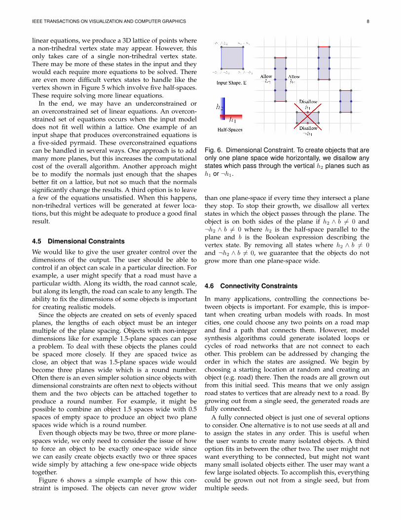
4.5 Dimensional Constraints

We would like to give the user greater control over thedimensions of the output. The user should be able tocontrol if an object can scale in a particular direction. Forexample, a user might specify that a road must have aparticular width. Along its width, the road cannot scale,but along its length, the road can scale to any length. Theability to fix the dimensions of some objects is importantfor creating realistic models.

Since the objects are created on sets of evenly spacedplanes, the lengths of each object must be an integermultiple of the plane spacing. Objects with non-integerdimensions like for example 1.5-plane spaces can posea problem. To deal with these objects the planes couldbe spaced more closely. If they are spaced twice asclose, an object that was 1.5-plane spaces wide wouldbecome three planes wide which is a round number.Often there is an even simpler solution since objects withdimensional constraints are often next to objects withoutthem and the two objects can be attached together toproduce a round number. For example, it might bepossible to combine an object 1.5 spaces wide with 0.5spaces of empty space to produce an object two planespaces wide which is a round number.

Even though objects may be two, three or more plane-spaces wide, we only need to consider the issue of howto force an object to be exactly one-space wide sincewe can easily create objects exactly two or three spaceswide simply by attaching a few one-space wide objectstogether.

Figure 6 shows a simple example of how this con-straint is imposed. The objects can never grow wider

Fig. 6. Dimensional Constraint. To create objects that areonly one plane space wide horizontally, we disallow anystates which pass through the vertical h2 planes such ash1 or ¬h1.

than one plane-space if every time they intersect a planethey stop. To stop their growth, we disallow all vertexstates in which the object passes through the plane. Theobject is on both sides of the plane if h2 ∧ b 6= 0 and¬h2 ∧ b 6= 0 where h2 is the half-space parallel to theplane and b is the Boolean expression describing thevertex state. By removing all states where h2 ∧ b 6= 0and ¬h2 ∧ b 6= 0, we guarantee that the objects do notgrow more than one plane-space wide.

4.6 Connectivity Constraints

In many applications, controlling the connections be-tween objects is important. For example, this is impor-tant when creating urban models with roads. In mostcities, one could choose any two points on a road mapand find a path that connects them. However, modelsynthesis algorithms could generate isolated loops orcycles of road networks that are not connect to eachother. This problem can be addressed by changing theorder in which the states are assigned. We begin bychoosing a starting location at random and creating anobject (e.g. road) there. Then the roads are all grown outfrom this initial seed. This means that we only assignroad states to vertices that are already next to a road. Bygrowing out from a single seed, the generated roads arefully connected.

A fully connected object is just one of several optionsto consider. One alternative is to not use seeds at all andto assign the states in any order. This is useful whenthe user wants to create many isolated objects. A thirdoption fits in between the other two. The user might notwant everything to be connected, but might not wantmany small isolated objects either. The user may want afew large isolated objects. To accomplish this, everythingcould be grown out not from a single seed, but frommultiple seeds.


4.7 Large-Scale ConstraintsWe would also like to give the user more control overthe large-scale structure of the output. The user mighthave a general idea of where certain types of objectsshould appear. Each object has a particular probabilitythat it will appear at any location in space. Generally, wechoose to give each state an equal probability of beingchosen, but we could easily modify the probabilitiesso that they are higher for any particular objects theuser wants to appear within some areas. The user couldeven set some probabilities to be zero in some places.If a state’s probability drops to zero, we can removeit entirely and then propagate the removal as usuallydone when assigning states (see Section 3.2). By chang-ing these probabilities, we can create cities and otherstructures in the shape of various symbols and otherobjects. We can also generate multiple outputs, evaluatehow well they match the user’s desired goal, and selectthe best output.

4.8 Algebraic Constraints and Bounding VolumesThe model synthesis algorithm creates a set of parallelplanes for every distinct normal of the input. As aresult, handling curved input models with many distinctnormals are computationally expensive because of thelarge number of planes that would have to be created.However, the number of distinct normals can be greatlyreduced by using bounding boxes and other boundingvolumes in place of complex objects. The algorithmcould be run using the bounding volumes in place ofthe input model and complex objects can be substitutedback into the output model M after it is generated.

There are several alternative ways the user can con-strain the dimensions. The object’s dimensions couldscale freely in a direction or be fixed (see Section 4.5).A third option is to let an object scale, but to requirethat it must scale uniformly in two or three directions.For example, the cylinder in Figure 7 only remainscylindrical if its x and y coordinates scale uniformlysx = sy . It is free to stretch along the z-coordinate by anyamount. To get its x and y coordinates to scale equally,we can place a bounding box around the cylinder andthe cut the box into two halves along the diagonalcreating two triangular prisms shown in Figure 7. Sincemodel synthesis scales triangular objects uniformly intwo dimensions, the output will be scaled identically inx and y, sx = sy and the cylinder can be substituted backin the shape.

The user may want to be even more restrictive andrequire the scalings be uniform in all directions sx =sy = sz . For example, the dome in Figure 7 remainsspherical only in this case. This can be accomplished byplacing a bounding box around the sphere and cuttingoff a tetrahedron as shown in Figure 7. Since modelsynthesis scales tetrahedra uniformly in all directions,the output will create a uniformly scaled copy of thebounding box.

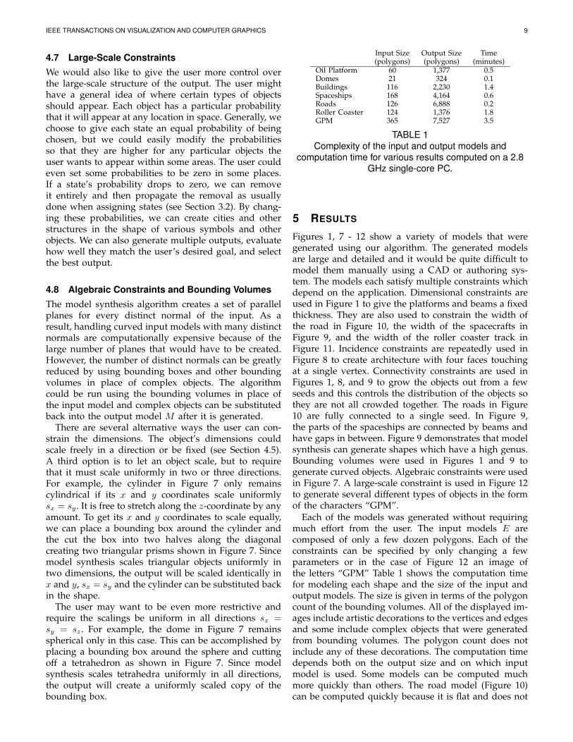
Input Size Output Size Time(polygons) (polygons) (minutes)

Oil Platform 60 1,377 0.5Domes 21 324 0.1Buildings 116 2,230 1.4Spaceships 168 4,164 0.6Roads 126 6,888 0.2Roller Coaster 124 1,376 1.8GPM 365 7,527 3.5

TABLE 1Complexity of the input and output models and

computation time for various results computed on a 2.8GHz single-core PC.

5 RESULTS

Figures 1, 7 - 12 show a variety of models that weregenerated using our algorithm. The generated modelsare large and detailed and it would be quite difficult tomodel them manually using a CAD or authoring sys-tem. The models each satisfy multiple constraints whichdepend on the application. Dimensional constraints areused in Figure 1 to give the platforms and beams a fixedthickness. They are also used to constrain the width ofthe road in Figure 10, the width of the spacecrafts inFigure 9, and the width of the roller coaster track inFigure 11. Incidence constraints are repeatedly used inFigure 8 to create architecture with four faces touchingat a single vertex. Connectivity constraints are used inFigures 1, 8, and 9 to grow the objects out from a fewseeds and this controls the distribution of the objects sothey are not all crowded together. The roads in Figure10 are fully connected to a single seed. In Figure 9,the parts of the spaceships are connected by beams andhave gaps in between. Figure 9 demonstrates that modelsynthesis can generate shapes which have a high genus.Bounding volumes were used in Figures 1 and 9 togenerate curved objects. Algebraic constraints were usedin Figure 7. A large-scale constraint is used in Figure 12to generate several different types of objects in the formof the characters “GPM”.

Each of the models was generated without requiringmuch effort from the user. The input models E arecomposed of only a few dozen polygons. Each of theconstraints can be specified by only changing a fewparameters or in the case of Figure 12 an image ofthe letters “GPM” Table 1 shows the computation timefor modeling each shape and the size of the input andoutput models. The size is given in terms of the polygoncount of the bounding volumes. All of the displayed im-ages include artistic decorations to the vertices and edgesand some include complex objects that were generatedfrom bounding volumes. The polygon count does notinclude any of these decorations. The computation timedepends both on the output size and on which inputmodel is used. Some models can be computed muchmore quickly than others. The road model (Figure 10)can be computed quickly because it is flat and does not


really use all three spatial dimensions. The ‘GPM’ modeltakes the longest time to compute because it uses severaldifferent input models including a spaceship model andseveral building models.

6 LIMITATIONS

The amount of time and memory that model synthesisneeds depends on the number of vertices. Vertices aregenerated wherever three or more planes intersect. Thenumber of planes depends on the number of distinctface normals. If there are n distinct normals and mparallel planes for each normal, there could be up toO(n3m3) vertices. The number of distinct normals canbe reduced by using bounding volumes, but only to acertain extent since bounding volumes can oversimplifysome objects. This makes generating curved objects us-ing model synthesis especially difficult [30]. A relatedproblem is that it is difficult to generate both largeand small objects simultaneously. Small objects requireclosely spaced planes while large objects require largevolumes which together means that many planes mustbe created.

Like most procedural modeling techniques, modelsynthesis is designed to work on objects that are self-similar. Model synthesis works best on objects withparts that identically match. Objects without identicalparts can be used with model synthesis, but they oftenproduce results that match the input too closely. Sincemodel synthesis is meant for digital entertainment andgaming, we assume that objects in the input are free fromsignificant errors in the vertex positions. Model synthesisworks efficiently on man-made structures that can berepresented with a few planar faces, but it has difficultywith organic and curved shapes.

Another limitation is that the objects often need tohave a grid structure. The grid is a necessary partof some of the constraints. The dimensional constraintassumes the dimensions fit on a grid. The incidenceconstraint assumes that the vertices can be fit onto a grid.The structure of the grid depends on the plane spacingwhich can be altered to accommodate some shapes, butnot all shapes as explained in Section 4.4. Some shapesmay produce an overconstrained set of equations whenusing Equation 4. Several strategies for dealing with thisproblem were discussed in Section 4.4, but each of themhas downsides.

7 COMPARISON

7.1 Prior Model Synthesis Algorithms

Previous model synthesis techniques [28] only use theadjacency constraint. Using prior algorithms without thedimensional and algebraic constraints, most of the re-sults would appear distorted and unnatural. Without theconnectivity constraint, the resulting models would con-tain mostly small crowded objects. Without the incidenceconstraints, none of the buildings in Figure 8 would

be generated. The large-scale constraint is required togenerate the pattern in Figure 12.

7.2 Other Procedural Modeling TechniquesEach of the model synthesis algorithms are semi-automatic. The user must perform several tasks. Thedifficulty of these tasks depends on the type of ob-ject that is being modeled. Objects that fit on a gridor contain mostly flat surfaces are relatively easy togenerate using model synthesis. These types of objectsare often man-made objects and are frequently foundin the architectural domain. But other shapes are moredifficult to generate using model synthesis includingmany natural and organic shapes. Organic shapes aredifficult to generate with model synthesis because theydo not fit on a grid and have many distinct normals.While model synthesis is not useful for generating everytype of objects, it offers benefits over other proceduralmethods for many classes of objects. The user has arelatively simple and straightforward objective: to findor to create an example model and describe a set ofconstraints on the output.

In contrast, the user’s objective is less simple andstraightforward for many existing procedural modelingtechniques. Many techniques require the user to con-struct a grammar. Given the shape of an object the userwants to model, there may not be a straightforward pro-cedure for constructing the rules of a grammar that couldgenerate a similar shape. Grammars are constructedthrough some human ingenuity and through trial anderror. The grammars themselves can be complicated,even when they describe simple shapes.

The model synthesis algorithms are easier to under-stand from a user’s perspective. The user does notneed to know anything about grammars or the innermechanics of the algorithm itself. The user only needsto know a few basic facts about the algorithm. The userdeals only with the input and output models and theconstraints. The user needs to avoid creating curvedsurfaces or to put bounding volumes around them. Oncea suitable example model has been created it is easy tomodify it as needed. Its parts can easily be rearrangedusing standard 3D modeling programs.

Most procedural modeling techniques are aimed atmodeling specific classes of objects such as urban build-ings [31], truss structures [39], fractals, and landscapes[32]. But many interesting structures lie outside of theseclasses of objects including spaceships, castles, oil plat-forms, plumbing, and roller coasters, just to name a few.Since model synthesis is a more general technique, itis especially useful for modeling objects that cannot begenerated easily using other techniques.

A close connection between model synthesis andcontext-sensitive grammars is demonstrated in Section7.3. Both methods can be used to accomplish the samegoal. The set of acceptable models can be represented bya grammar, but it is different in several ways from gram-mars that are typically used in procedural modeling. The


location of empty space is recorded in model synthesis.Empty space is not explicitly recorded in most grammar-based techniques. It is determined by checking that allof the objects are absent. Model synthesis algorithms arealso good at avoiding self-intersections which is part ofthe adjacency constraint. The grammars found in othertechniques may need to be carefully constructed so thatself-intersections do not occur. Another task that modelsynthesis is particularly good at is in creating closedpaths such as Figure 10.

A method [5] closely related to model synthesis auto-matically detects symmetrical parts and derives a shapegrammar. This method complements work in model syn-thesis since the user would not need to label symmetricalparts if this were computed automatically. Like othershape grammars, the derived shape grammar can notalways anticipate and avoid self-intersections and mayhave difficulty forming closed paths.

Model synthesis algorithms are good at creating ge-ometric detail at a particular scale, but not at multiplescales. For example, it is difficult for model synthesis tocreate geometric detail at the scale of a building and atthe scale of the building’s window or door knob simul-taneously. Other grammar-based methods [31], [25], [32]create geometric detail at multiple scales more easily.

7.3 Relationship between model synthesis and Con-text Sensitive Grammars

The problem of deciding if a string is part of the contextsensitive language L can be reduced to a problem ofdeciding if a model containing that string satisfies theadjacency constraint. A model is consistent if it it satisfiesthe adjacency constraint.

For every context-sensitive language L, there is alinear-bounded automaton that accepts L. It can beshown that all of the actions of a linear-bounded au-tomaton A accepting a string can be described within aconsistent model.

For any linear bounded automaton, an adjacency con-straint can be constructed such that the model that isgenerated will reproduce the actions of the automaton.Each row of the model records the symbols on the tape,the location of the tape head, and the state of A. Forexample, suppose the problem is to determine if thestring ‘aabbcc’ is in the language {aibici|i ≥ 1}. The tapewould initially contain this input string along with twosymbols ‘<’ and ‘>’ to mark the start and end of thetape. The width of the model M is equal to the width ofthe tape. The first row of the model would contain thelabels

Row 1: < (a,q0) a b b c c >

The label (a,q0) is used to indicate that the automaton Ais in its initial state q0 and the tape head is reading the ‘a’symbol. For every state q and every symbol in the tapealphabet s, there is a label (q, s). Suppose that when A isin state q0 and is reading symbol ‘a’ that it responds by

printing the symbol ‘d’ onto the tape, switching to stateq1, and remaining stationary. Then the model’s next rowwould be

Row 2: < (d,q1) a b b c c >

An adjacency constraint can be constructed whichwould guarantee that this row would appear beneathrow 1. The constaint is constructed to allow only onepossible option at every location which is exactly theoption that the automaton would choose. The constraintcan be constructed so that the tape head also movesto the left or to the right. The problem of determiningif a string is part of a context-sensitive language canbe decided by determining if such a model can becompleted acceptably. This gives an overview of theproof. More details can be found in [27].

We have discussed how a context-sensitive grammarproblem can be reduced to a model synthesis problem.The reverse is also true. A context-sensitive grammarcan be used to generate consistent models. For everyexample model E there is a linear-bounded automatonthat can examine all of the labels in the model and verifythat all adjacency labels satisfy the adjacency constraint.This topic is explored in more detail in [27].

8 CONCLUSION AND FUTURE WORK

We have presented several major improvements tomodel synthesis that allow the user to more effectivelycontrol the output. We enable the user to fix dimensionsof objects, to specify a large-scale structure of the output,to produce connected results, to add bounding volumes,to have multiple object interiors, and to generate shapeswith complex vertex states. Further work is needed toimprove the efficiency of model synthesis, especiallywhen generating large and small objects together. Morework is needed for handling curved objects beyondusing bounding volumes [30]. One important constraintthat is still missing is one to create symmetrical objects.

ACKNOWLEDGEMENTS

We would like to thank the reviewers for theircomments. This work was supported in part byARO Contract W911NF-04-1-0088, NSF awards 0636208,0917040 and 0904990, and DARPA/RDECOM ContractWR91CRB-08-C-0137.

BIOGRAPHY

Paul Merrell is currently a Postdoctoral Scholar at Stan-ford University. He received his Ph.D. in ComputerScience at the University of North Carolina at ChapelHill in 2009. He also received a Bachelor’s and Mas-ter’s degree in Electrical Engineering at Brigham YoungUniversity. Paul Merrell has worked on many projectsin computer graphics and computer vision and spentseveral summers working at EA Games and RaytheonMissile Systems.


Dinesh Manocha is currently the Phi DeltaTheta/Mason Distinguished Professor of ComputerScience at the University of North Carolina at ChapelHill. He received his Ph.D. in Computer Scienceat the University of California at Berkeley 1992.He has received Junior Faculty Award, Alfred P. SloanFellowship, NSF Career Award, Office of Naval ResearchYoung Investigator Award, Honda Research InitiationAward, Hettleman Prize for Scholarly Achievement.Along with his students, Manocha has also received 12best paper & panel awards at the leading conferences ongraphics, geometric modeling, visualization, multimediaand high-performance computing. He is an ACM Fellow.

Manocha has published more than 280 papers in theleading conferences and journals on computer graphics,geometric computing, robotics, and scientific computing.He has also served as a program committee memberand program chair for more than 75 conferences in theseareas, and editorial boards of many leading journals.Some of the software systems related to collision detec-tion, GPU-based algorithms and geometric computingdeveloped by his group have been downloaded by morethan 100,000 users and are widely used in the industry.He has supervised 18 Ph.D. dissertations.

REFERENCES

[1] H. Ault, “Using geometric constraints to capture design intent,” Journal forGeometry and Graphics, vol. 3, no. 1, pp. 39–47, 1999.

[2] D. G. Aliaga, C. A. Vanegas, and B. Benes, “Interactive example-based urbanlayout synthesis,” ACM Trans. Graph., vol. 27, no. 5, pp. 1–10, 2008.

[3] C. Barnes, E. Shechtman, A. Finkelstein, and D. B. Goldman, “PatchMatch: Arandomized correspondence algorithm for structural image editing,” ACMTransactions on Graphics (Proc. SIGGRAPH), vol. 28, no. 3, Aug. 2009.

[4] P. Bhat, S. Ingram, and G. Turk, “Geometric texture synthesis by example,”in SGP ’04: Symposium on Geometry processing. New York, NY, USA: ACM,2004, pp. 41–44.

[5] M. Bokeloh, M. Wand, H. Seidel, “A Connection between Partial Symmetryand Inverse Procedural Modeling,” in Proc. of ACM SIGGRAPH, 2010.

[6] W. Bouma, I. Fudos, C. Hoffmann, J. Cai, and R. Paige, “A geometricconstraint solver,” Computer-Aided Design, vol. 27, no. 6, pp. 487–501, 1995.

[7] G. Chen, G. Esch, P. Wonka, P. Muller, and E. Zhang, “Interactive proceduralstreet modeling,” ACM Trans. Graph., vol. 27, no. 3, 2008.

[8] X. Chen, B. Neubert, Y.-Q. Xu, O. Deussen, and S. B. Kang, “Sketch-basedtree modeling using markov random field,” ACM Trans. Graph., vol. 27, no. 5,pp. 1–9, 2008.

[9] B. Cutler, J. Dorsey, L. McMillan, M. Muller, and R. Jagnow, “A proceduralapproach to authoring solid models,” ACM Trans. Graph., vol. 21, no. 3, pp.302–311, 2002.

[10] A. A. Efros and W. T. Freeman, “Image quilting for texture synthesis andtransfer,” in SIGGRAPH ’01. New York, NY, USA: ACM, 2001, pp. 341–346.

[11] A. A. Efros and T. K. Leung, “Texture synthesis by non-parametric sam-pling,” in IEEE International Conference on Computer Vision, Corfu, Greece,September 1999, pp. 1033–1038.

[12] U. Flemming, “More than the sum of parts: the grammar of queen annehouses,” Environment and Planning B: Planning and Design, vol. 14, no. 3, pp.323–350, May 1987.

[13] A. Fournier, D. Fussell, and L. Carpenter, “Computer rendering of stochasticmodels,” Commun. ACM, vol. 25, no. 6, pp. 371–384, 1982.

[14] T. Funkhouser, M. Kazhdan, P. Shilane, P. Min, W. Kiefer, A. Tal,S. Rusinkiewicz, and D. Dobkin, “Modeling by example,” SIGGRAPH ’04,2004.

[15] C. M. Hoffmann and J. R. Rossignac, “A road map to solid modeling,”IEEE Transactions on Visualization and Computer Graphics, vol. 2, no. 1, pp.3–10, 1996.

[16] C. M. Hoffmann, A. Lomonosov, and M. Sitharam, “Geometric constraintdecomposition,” in Geometric Constraint Solving, B. Bruderlin and D. Roller,Eds. Springer-Verlag, 1998, pp. 170–195.

[17] T. Igarashi, S. Matsuoka, and H. Tanaka, “Teddy: a sketching interface for3d freeform design,” in Proc. of ACM SIGGRAPH ’99. New York, NY, USA:ACM Press/Addison-Wesley Publishing Co., 1999, pp. 409–416.

[18] G. A. Kramer and B. B. Qh, “Solving geometric constraint systems.” MITPress, 1992, pp. 708–714.

[19] J. Kopf, C.-W. Fu, D. Cohen-Or, O. Deussen, D. Lischinski, and T.-T. Wong,“Solid texture synthesis from 2d exemplars,” ACM Trans. Graph., vol. 26,no. 3, p. 2, 2007.

[20] V. Kwatra, A. Schodl, I. Essa, G. Turk, and A. Bobick, “Graphcut textures:image and video synthesis using graph cuts,” in SIGGRAPH ’03. New York,NY, USA: ACM, 2003, pp. 277–286.

[21] J. Legakis, J. Dorsey, and S. Gortler, “Feature-based cellular texturing forarchitectural models,” in Proc. Of ACM SIGGRAPH ’01, 2001, pp. 309–316.

[22] A. Lindenmayer, “Mathematical models for cellular interactions in develop-ment i. filaments with one-sided inputs,” Journal of Theoretical Biology, vol. 18,no. 3, pp. 280–299, March 1968.

[23] B. B. Mandelbrot, The Fractal Geometry of Nature. W. H. Freeman, August1982.

[24] N. J. Mitra, L. Guibas, and M. Pauly, “Partial and approximate symmetrydetection for 3d geometry,” in ACM Transactions on Graphics, vol. 25, no. 3,2006, pp. 560–568.

[25] R. Mech and P. Prusinkiewicz, “Visual models of plants interacting withtheir environment,” in Proc. Of ACM SIGGRAPH ’96, 1996, pp. 397–410.

[26] P. Merrell, “Example-based model synthesis,” in I3D ’07: Symposium onInteractive 3D graphics and games. ACM Press, 2007, pp. 105–112.

[27] P. Merrell, “Model synthesis,” Ph.D. dissertation, University of NorthCarolina at Chapel Hill, 2009.

[28] P. Merrell and D. Manocha, “Continuous model synthesis,” Proc. of ACMSIGGRAPH ASIA ’08, 2008.

[29] P. Merrell and D. Manocha, “Constraint-based model synthesis,” in SPM ’09:2009 SIAM/ACM Joint Conference on Geometric and Physical Modeling. NewYork, NY, USA: ACM, 2009, pp. 101–111.

[30] P. Merrell and D. Manocha, “Example-based curve synthesis,” in Computers& Graphics. (To Appear).

[31] P. Muller, P. Wonka, S. Haegler, A. Ulmer, and L. V. Gool, “Proceduralmodeling of buildings,” ACM Trans. Graph., vol. 25, no. 3, pp. 614–623, 2006.

[32] F. K. Musgrave, C. E. Kolb, and R. S. Mace, “The synthesis and renderingof eroded fractal terrains,” in Proc. Of ACM SIGGRAPH ’89, 1989, pp. 41–50.

[33] A. Nealen, T. Igarashi, O. Sorkine, and M. Alexa, “Fibermesh: designingfreeform surfaces with 3d curves,” Proc. of ACM SIGGRAPH ’07, vol. 26,no. 3, p. 41, 2007.

[34] Y. Parish and P. Muller. “Procedural modeling of cities,” Proc. of ACMSIGGRAPH ’01, pp. 301–308, New York, NY, USA, 2001.

[35] H. Pottmann, Y. Liu, J. Wallner, A. Bobenko, and W. Wang, “Geometry ofmulti-layer freeform structures for architecture,” Proc. Of ACM SIGGRAPH’07, 2007.

[36] P. Prusinkiewicz, A. Lindenmayer, and J. Hanan, “Development modelsof herbaceous plants for computer imagery purposes,” SIGGRAPH Comput.Graph., vol. 22, no. 4, pp. 141–150, 1988.

[37] P. Prusinkiewicz, L. Mundermann, R. Karwowski, and B. Lane, “The useof positional information in the modeling of plants,” in Proc. Of ACMSIGGRAPH ’01, 2001, pp. 289–300.

[38] L. Quan, P. Tan, G. Zeng, L. Yuan, J. Wang, and S. B. Kang, “Image-basedplant modeling,” ACM Trans. Graph., vol. 25, no. 3, pp. 599–604, 2006.

[39] J. Smith, J. Hodgins, I. Oppenheim, and A. Witkin, “Creating models oftruss structures with optimization,” ACM Trans. Graph., vol. 21, no. 3, pp.295–301, 2002.

[40] G. Stiny and W. J. Mitchell, “The palladian grammar,” Environment andPlanning B: Planning and Design, vol. 5, no. 1, pp. 5–18, January 1978.

[41] P. Torrens, David, and Sullivan, “Cellular automata and urban simulation:where do we go from here?” Environment and Planning B: Planning andDesign, vol. 28, no. 2, pp. 163–168, March 2001.

[42] G. Turk, “Texture synthesis on surfaces,” in SIGGRAPH ’01. New York,NY, USA: ACM, 2001, pp. 347–354.

[43] C. Vanegas, D. Aliaga, P. Wonka, P. Muller, P. Waddell, and B. Watson,“Modeling the appearance and behavior of urban spaces,” in Eurographics2009, State of the Art Report, EG-STAR. Eurographics Association, 2009.

[44] P. Waddell, “Urbansim: Modeling urban development for land use, trans-portation and environmental planning,” Journal of the American PlanningAssociation, vol. 68, pp. 297–314, 2002.

[45] B. Watson, P. Muller, O. Veryovka, A. Fuller, P. Wonka, and C. Sexton,“Procedural urban modeling in practice,” IEEE Comput. Graph. Appl., vol. 28,no. 3, pp. 18–26, 2008.

[46] B. Weber, P. Mueller, P. Wonka, and M. Gross, “Interactive geometricsimulation of 4d cities,” Computer Graphics Forum, April 2009.

[47] L.-Y. Wei, S. Lefebvre, V. Kwatra, and G. Turk, “State of the art in example-based texture synthesis,” in Eurographics 2009, State of the Art Report, EG-STAR. Eurographics Association, 2009.

[48] L.-Y. Wei and M. Levoy, “Fast texture synthesis using tree-structured vectorquantization,” in Proc. Of ACM SIGGRAPH ’00, 2000, pp. 479–488.

[49] P. Wonka, M. Wimmer, F. Sillion, and W. Ribarsky, “Instant architecture,”in Proc. Of ACM SIGGRAPH ’03, 2003, pp. 669–677.

[50] H. Zhou and J. Sun, “Terrain synthesis from digital elevation models,” IEEETransactions on Visualization and Computer Graphics, vol. 13, no. 4, pp. 834–848,2007.

[51] K. Zhou, X. Huang, X. Wang, Y. Tong, M. Desbrun, B. Guo, and H.-Y. Shum,“Mesh quilting for geometric texture synthesis,” in SIGGRAPH, pp. 690–697,2006.


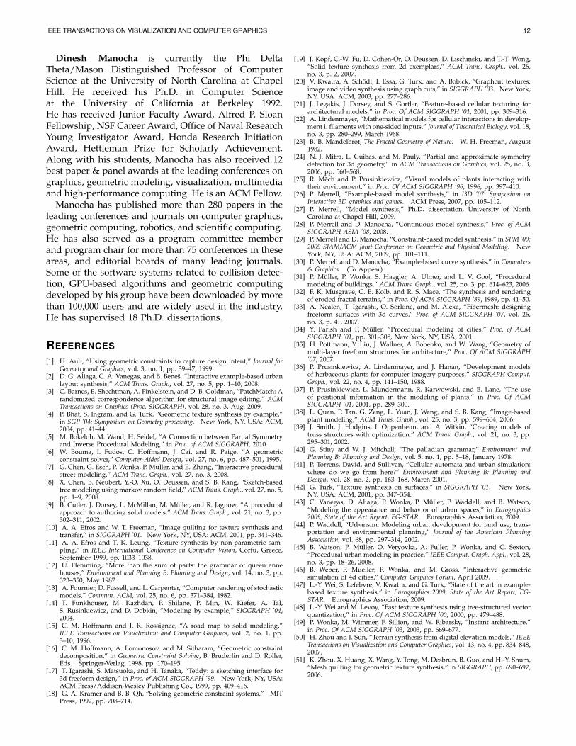
(a) Input (b) Output with Bounding Volumes (c) Output without Bounding Volumes

Fig. 7. Because model synthesis is inefficient on curved models bounding volumes are used to simplify the geometry(a). The bounding boxes are cut into two objects, so the dome will scale uniformly and the cylinder will scale uniformlyin x and y. The output is generated and the complex original shapes are substituted back in (b,c).

(a) Input Model (b) Output Model

Fig. 8. Many complex buildings (b) are generated from four simple ones (a). The output contains many verticesthat have been constrained to intersect four faces and a few of these vertices are circled. The result also usesthe connectivity constraint to space the buildings apart which gives the buildings more room to develop into moreinteresting shapes.

Fig. 9. A fleet of spaceships (b,c) is automatically generated from a simple spaceship model (a). Without theconnectivity constraint several dozen small unconnected spaceships are generated (b), but they are all packedtogether. With the connectivity constraint, six large spaceships are generated (c). Dimensional constraints areextensively used to ensure the rocket engines and other structures do not stretch unnaturally. The shape of thespaceships have a high genus because there are gaps in between the beams and parts of the spaceships.


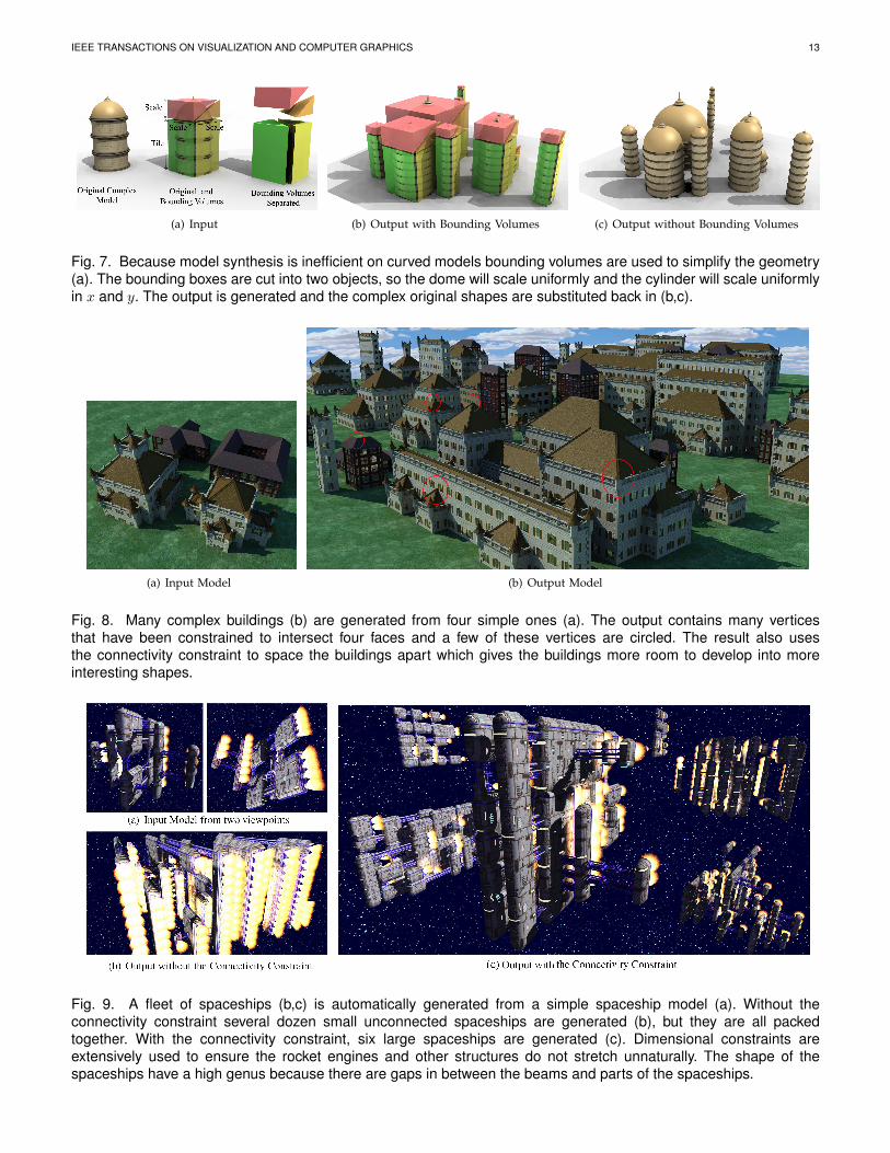
(a) Input (b) Output

Fig. 10. A large fully connected road network is generated (b) from a few streets using the connectivity constraint.The dimensions of the roads are also constrained.

(a) Input Model (b) Output Model

Fig. 11. Several long roller coasters (b) are generated from one simple ones (a). Dimensional constraints are used tokeep the track a certain width.

Fig. 12. Large-scale constraints are used to build spaceships in the shape of the letter ‘G’, rectangular buildings inthe shape of the letter ‘P’, and buildings from Figure 8 in the shape of the letter ‘M’.

Documents

IEEE TRANSACTIONS ON VISUALIZATION AND COMPUTER GRAPHICS …graphics.stanford.edu/~pmerrell/tvcg.pdf · IEEE TRANSACTIONS ON VISUALIZATION AND COMPUTER GRAPHICS 1 ... A General Procedural