Computer graphics & visualization Fluids. computer graphics & visualization Simulation and Animation – SS 07 Jens Krüger – Computer Graphics and Visualization

computer graphics & visualization

Simulation and Animation

Fluids


Simulation and Animation – SS 07Jens Krüger – Computer Graphics and Visualization Group

Fluid simulation• Content

– Fluid simulation basics • Terminology • Navier-Stokes equations• Derivation and physical interpretation

– Computational fluid dynamics• Discretization• Solution methods



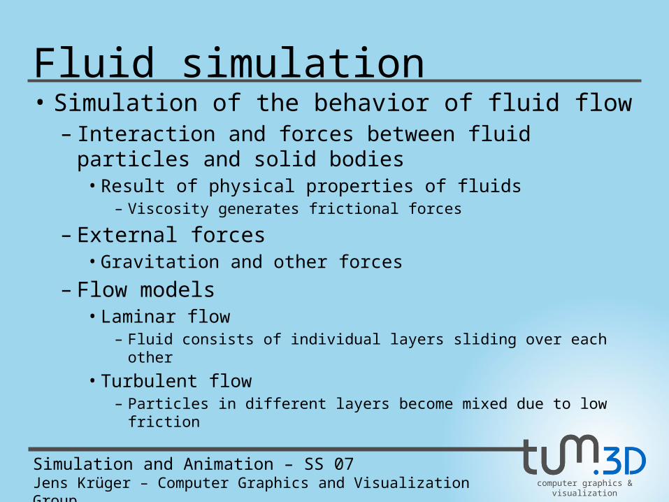
Fluid simulation• Simulation of the behavior of fluid flow

– Interaction and forces between fluid particles and solid bodies

• Result of physical properties of fluids– Viscosity generates frictional forces

– External forces• Gravitation and other forces

– Flow models• Laminar flow

– Fluid consists of individual layers sliding over each other

• Turbulent flow – Particles in different layers become mixed due to low friction



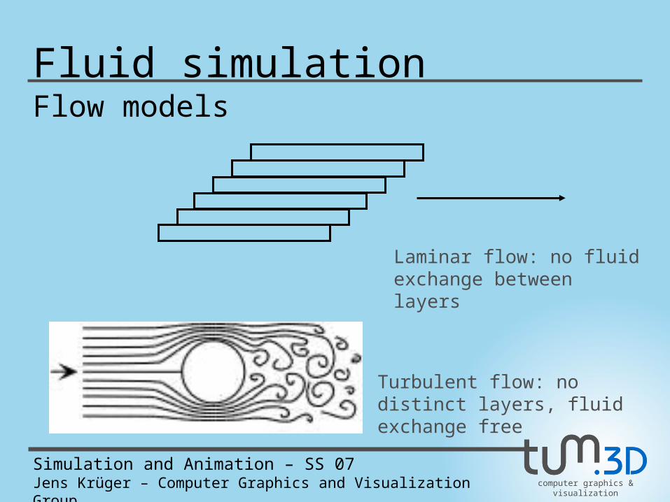
Fluid simulationFlow models

Laminar flow: no fluid exchange between layers

Turbulent flow: no distinct layers, fluid exchange free



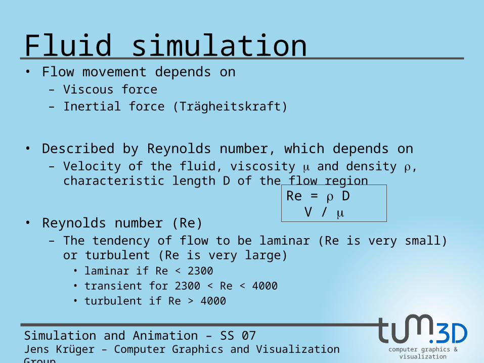
Fluid simulation• Flow movement depends on

– Viscous force– Inertial force (Trägheitskraft)

• Described by Reynolds number, which depends on– Velocity of the fluid, viscosity and density , characteristic length D of the flow

region

• Reynolds number (Re)– The tendency of flow to be laminar (Re is very small) or turbulent (Re is very

large)• laminar if Re < 2300 • transient for 2300 < Re < 4000 • turbulent if Re > 4000

Re = D V /



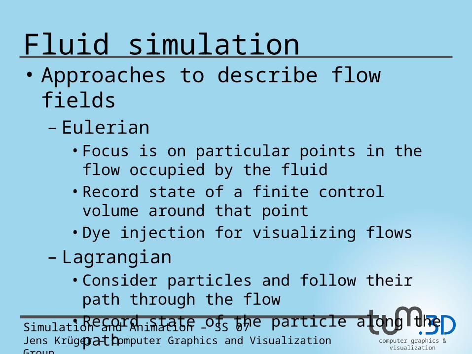
Fluid simulation• Approaches to describe flow fields

– Eulerian• Focus is on particular points in the flow occupied by the

fluid• Record state of a finite control volume around that point• Dye injection for visualizing flows

– Lagrangian• Consider particles and follow their path through the flow• Record state of the particle along the path• Particle tracing for visualizing flows



Fluid simulation• Basic equations of fluid dynamics

– Rely on• Physical principles

– Conservation of mass– F=ma– Conservation of energy

• Applied to a model of the flow– Finite control volume approach– Infinitesimal particle approach

• Derivation of mathematical equations– Continuity equation– Navier-Stokes equations



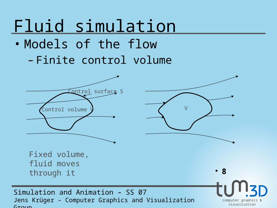
Fluid simulation• Models of the flow

– Finite control volume

• 8

Control volume V

Control surface S

V

Fixed volume, fluid moves through it



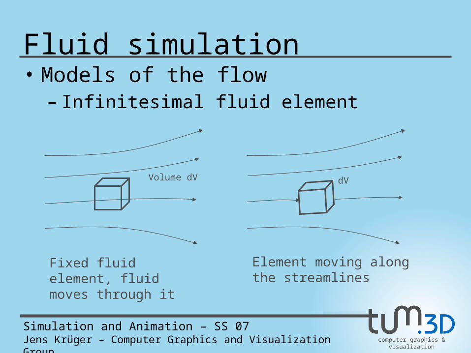
Fluid simulation• Models of the flow

– Infinitesimal fluid element

dV

Fixed fluid element, fluid moves through it

Element moving along the streamlines

Volume dV



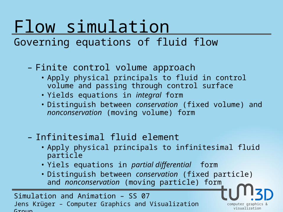
Flow simulationGoverning equations of fluid flow

– Finite control volume approach• Apply physical principals to fluid in control volume and passing

through control surface• Yields equations in integral form• Distinguish between conservation (fixed volume) and

nonconservation (moving volume) form

– Infinitesimal fluid element• Apply physical principals to infinitesimal fluid particle• Yiels equations in partial differential form• Distinguish between conservation (fixed particle) and

nonconservation (moving particle) form



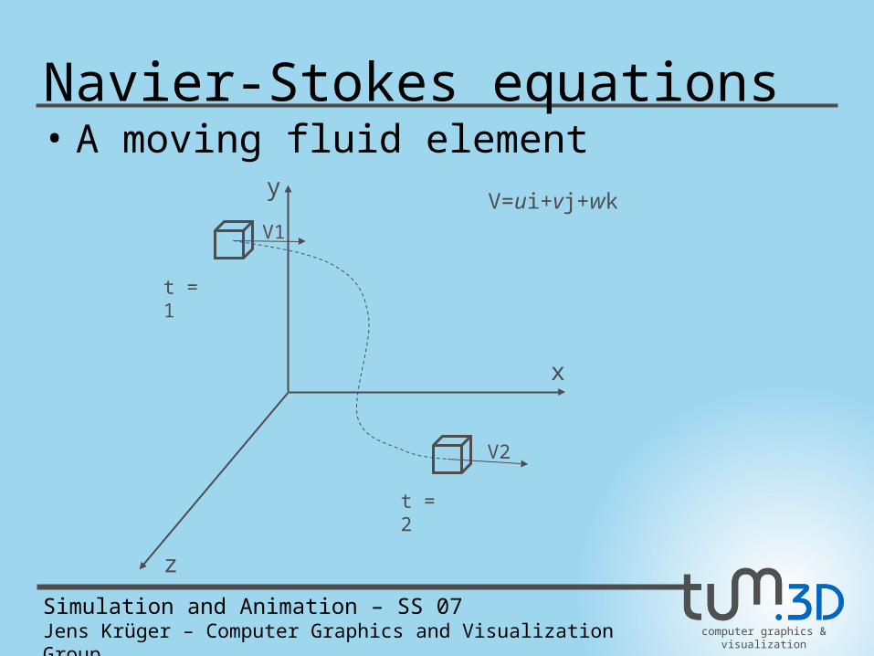
Navier-Stokes equations• A moving fluid element

x

z

y

V1

V2

t = 1

t = 2

V=ui+vj+wk



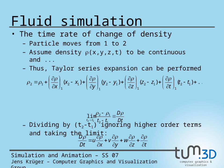
Fluid simulation• The time rate of change of density

– Particle moves from 1 to 2– Assume density (x,y,z,t) to be continuous and ...– Thus, Taylor series expansion can be performed

– Dividing by (t2-t1) ignoring higher order termsand taking the limit:

...)()()()( 121

121

12

1

121

12

ttt

zzz

yyy

xxx

Dt

D

tttt

12

12

12

lim

tzw

yv

xu

Dt

D



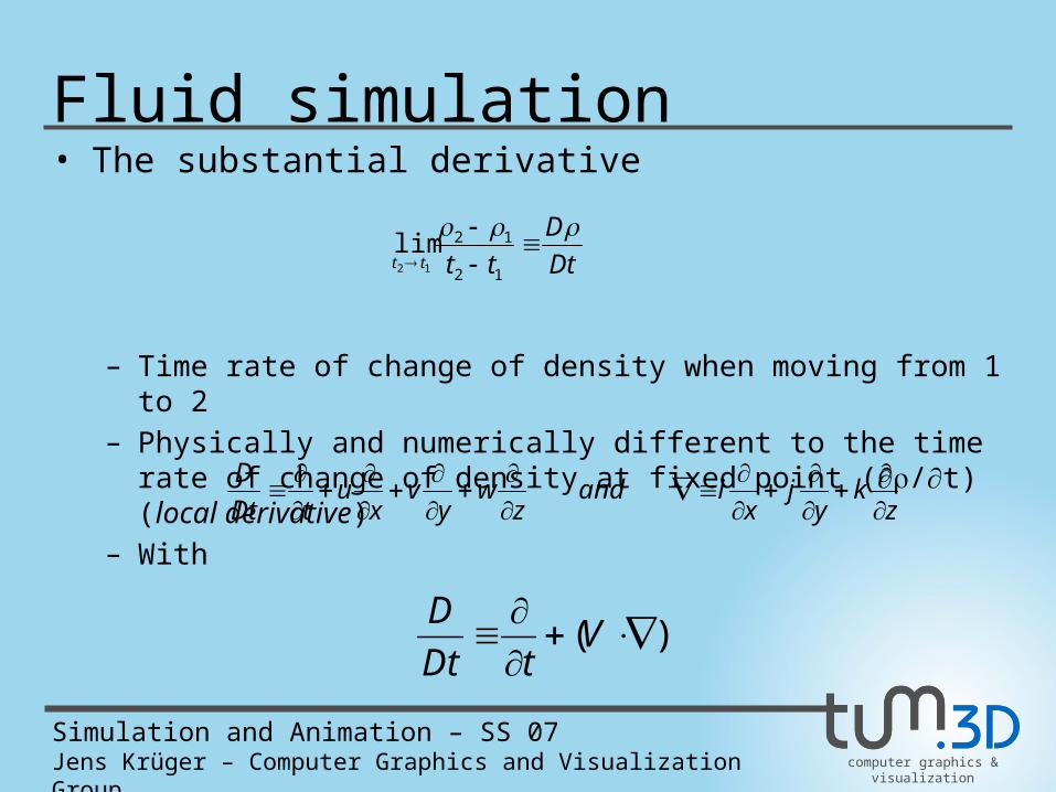
Fluid simulation• The substantial derivative

– Time rate of change of density when moving from 1 to 2– Physically and numerically different to the time rate of change of density

at fixed point (/t) (local derivative)– With

zk

yj

xiand

zw

yv

xu

tDt

D

Dt

D

tttt

12

12

12

lim

)(

VtDt

D



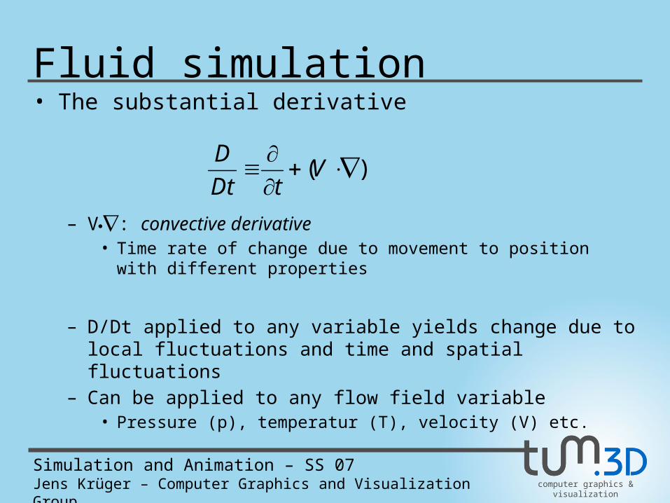
Fluid simulation• The substantial derivative

– V: convective derivative• Time rate of change due to movement to position with different properties

– D/Dt applied to any variable yields change due tolocal fluctuations and time and spatial fluctuations

– Can be applied to any flow field variable • Pressure (p), temperatur (T), velocity (V) etc.

)(

VtDt

D



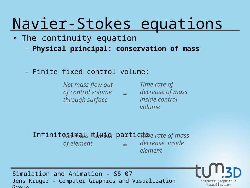
Navier-Stokes equations• The continuity equation

– Physical principal: conservation of mass

– Finite fixed control volume:

– Infinitesimal fluid particle

Net mass flow out of control volume through surface

Time rate of decrease of mass inside control volume

=

Net mass flow out of element

Time rate of mass decrease inside element

=



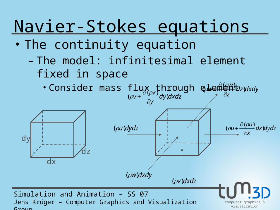
Navier-Stokes equations• The continuity equation

– The model: infinitesimal element fixed in space• Consider mass flux through element

dx

dy

dz

dydzu)( dydzdxx

uu )

)((

dxdzv)(dxdyw)(

dxdydzz

ww )

)((

dxdzdyy

vv )

)((



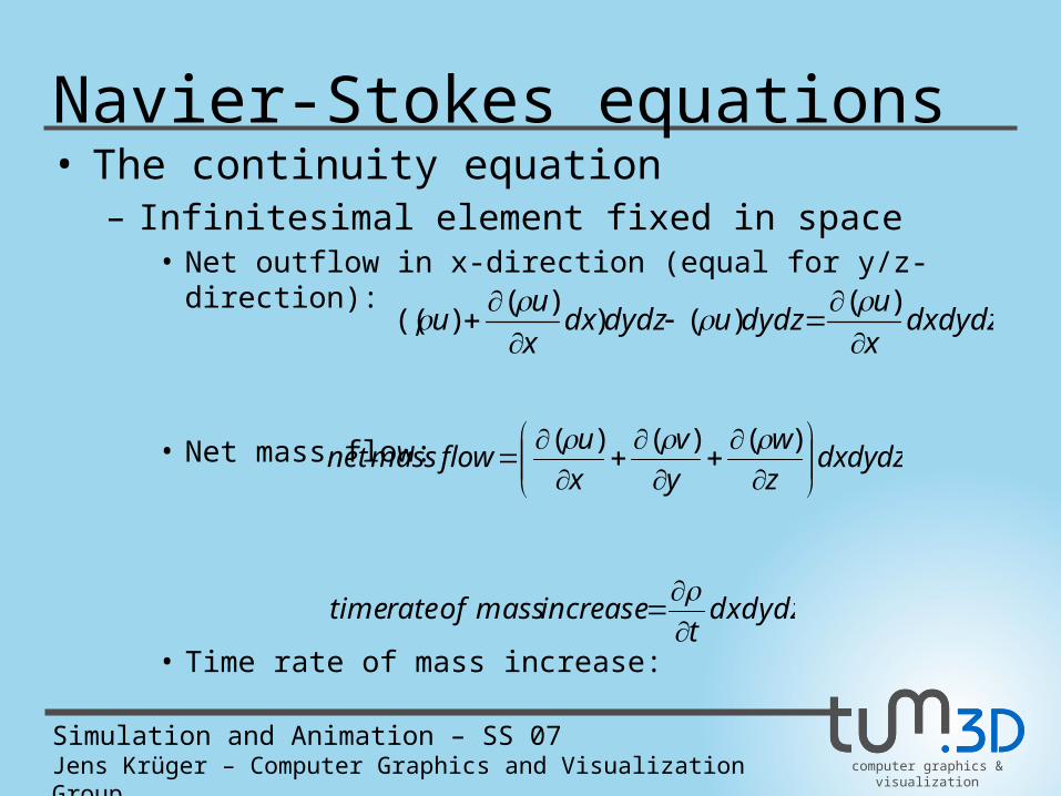
Navier-Stokes equations • The continuity equation

– Infinitesimal element fixed in space• Net outflow in x-direction (equal for y/z-direction):

• Net mass flow:

• Time rate of mass increase:

dxdydzx

udydzudydzdx

x

uu

)()()

)()((

dxdydzz

w

y

v

x

uflowmassnet

)()()(

dxdydzt

increasemassofratetime



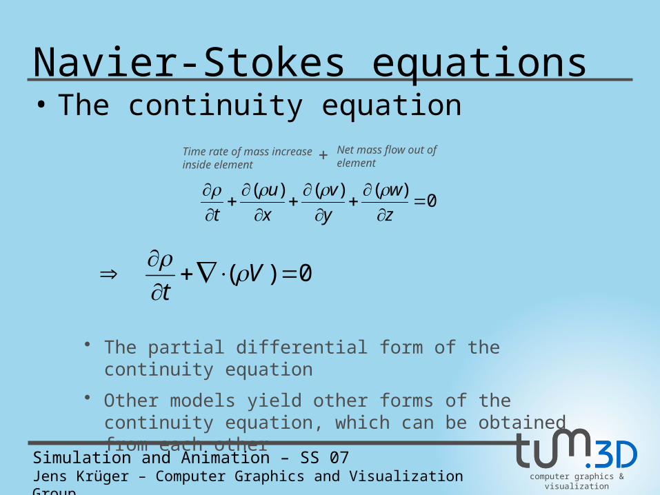
Navier-Stokes equations • The continuity equation

0)()()(

z

w

y

v

x

u

t

0)(

Vt

• The partial differential form of the continuity equation

• Other models yield other forms of the continuity equation, which can be obtained from each other

Time rate of mass increase inside element

Net mass flow out of element+



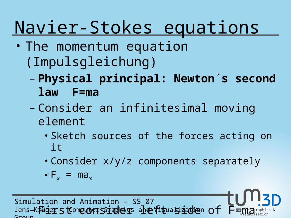
Navier-Stokes equations • The momentum equation (Impulsgleichung)

– Physical principal: Newton´s second law F=ma– Consider an infinitesimal moving element

• Sketch sources of the forces acting on it• Consider x/y/z components separately• Fx = max

– First consider left side of F=ma• F = FB + FS

• Sum of body forces and surface forces acting on element



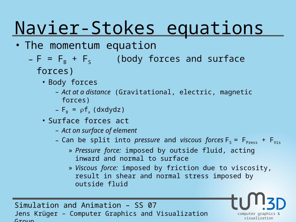
Navier-Stokes equations• The momentum equation

– F = FB + FS (body forces and surface forces)• Body forces

– Act at a distance (Gravitational, electric, magnetic forces)– FB = fx (dxdydz)

• Surface forces act– Act on surface of element– Can be split into pressure and viscous forces FS = FPress + FVis

» Pressure force: imposed by outside fluid, acting inward and normal to surface

» Viscous force: imposed by friction due to viscosity, result in shear and normal stress imposed by outside fluid



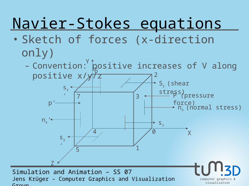
Navier-Stokes equations• Sketch of forces (x-direction only)

– Convention: positive increases of V along positive x/y/z

X

Y

Z

0

1

2

3

4

5

6

7 P (pressure force)p‘

Sy (shear stress)

sy‘

nx (normal stress)

nx‘ sz

sz‘



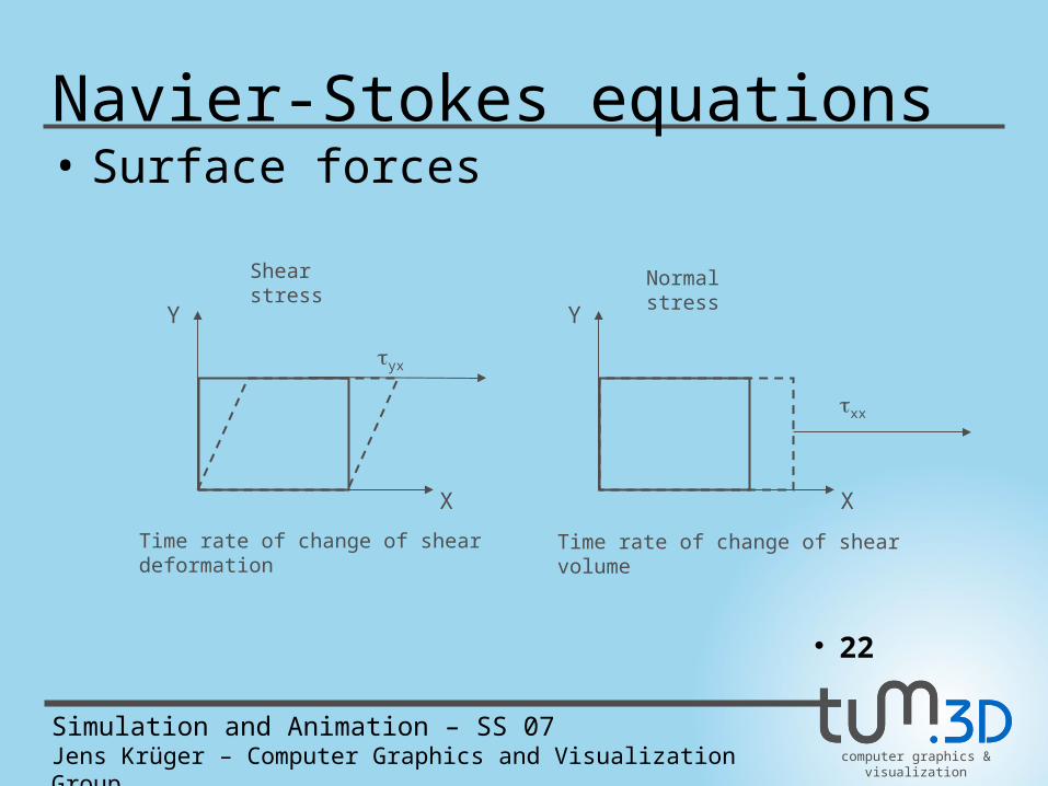
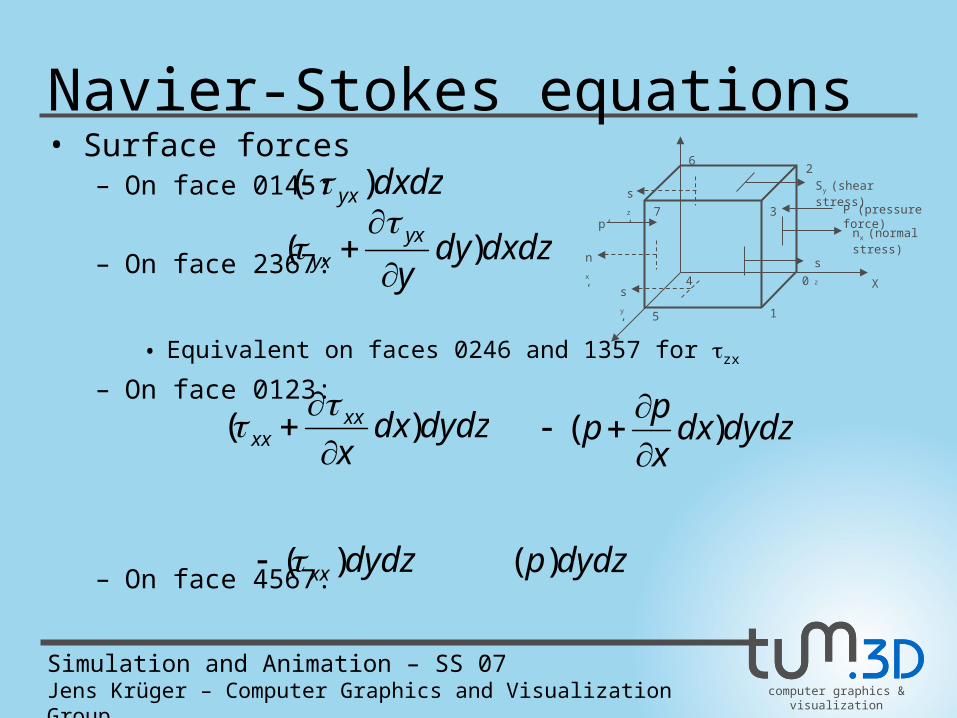
Navier-Stokes equations• Surface forces

• 22

X

Y

yx

X

Y

xx

Time rate of change of shear deformation Time rate of change of shear volume

Shear stress Normal stress



Navier-Stokes equations• Surface forces

– On face 0145:

– On face 2367:

• Equivalent on faces 0246 and 1357 for zx

– On face 0123:

– On face 4567:

dxdzyx )(

dxdzdyyyx

yx )(

dydzdxxxx

xx )(

dydzdx

x

pp )(

dydzxx )( dydzp)(

X0

1

2

3

4

5

6

7 P (pressure force)p‘

Sy (shear stress)

s

y

‘

nx (normal stress)

n

x‘ s

z

s

z

‘



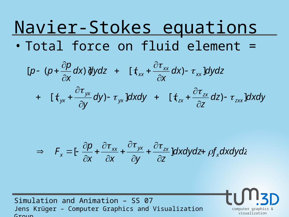
Navier-Stokes equations• Total force on fluid element =

dxdydzz

dxdydyy

dydzdxx

dydzdxx

ppp

zxxzx

zxyxyx

yx

xxxx

xx

])[(])[(

])[()]([

dxdydzfdxdydzzyxx

pF x

zxyxxxx

][



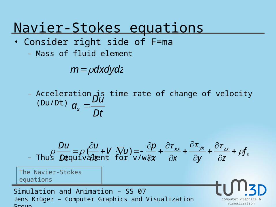
Navier-Stokes equations• Consider right side of F=ma

– Mass of fluid element

– Acceleration is time rate of change of velocity (Du/Dt)

– Thus (equivalent for v/w):

dxdydzm

Dt

Duax

xzxyxxx fzyxx

puV

t

u

Dt

Du

)(

The Navier-Stokes equations



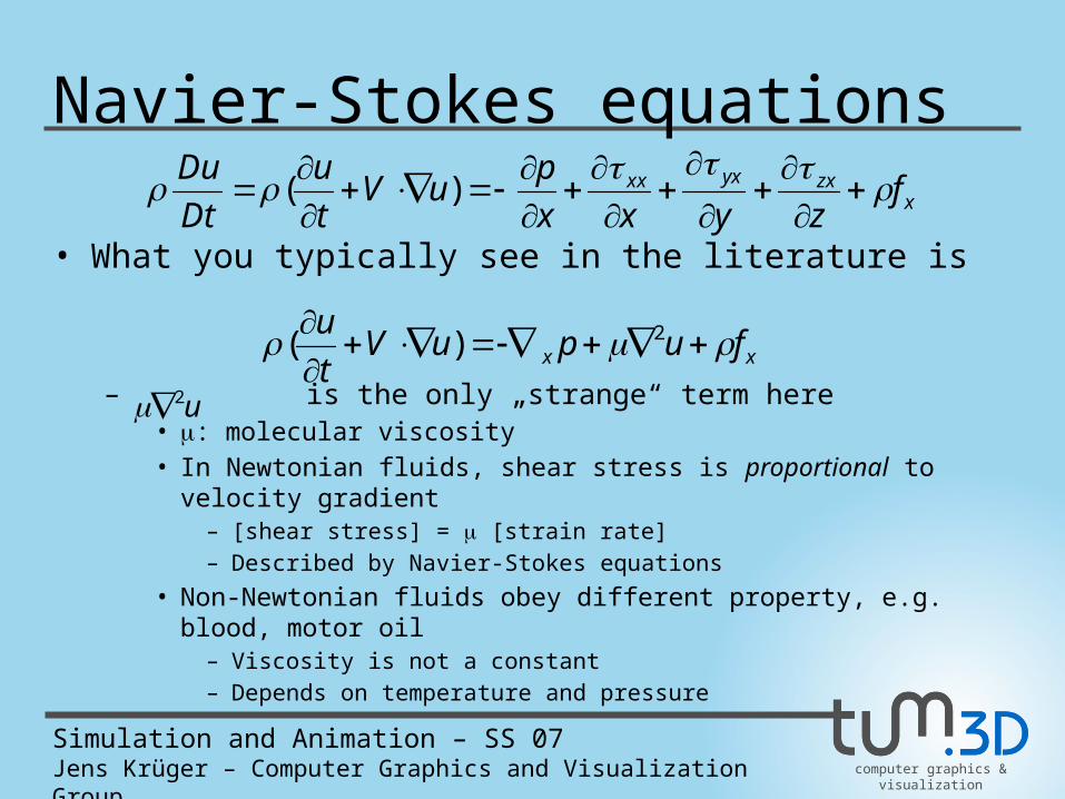
Navier-Stokes equations

• What you typically see in the literature is

– is the only „strange“ term here• : molecular viscosity• In Newtonian fluids, shear stress is proportional to velocity gradient

– [shear stress] = [strain rate]– Described by Navier-Stokes equations

• Non-Newtonian fluids obey different property, e.g. blood, motor oil– Viscosity is not a constant– Depends on temperature and pressure

xx fupuVt

u 2)(

u2

xzxyxxx fzyxx

puV

t

u

Dt

Du

)(



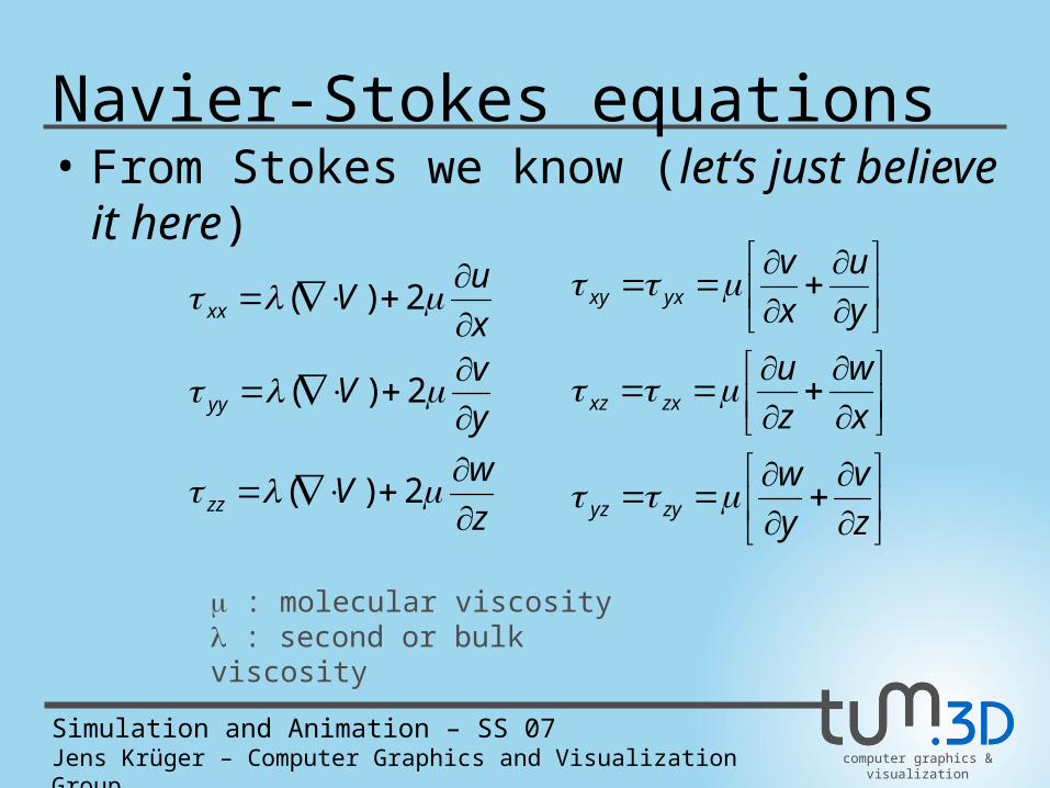
Navier-Stokes equations• From Stokes we know (let‘s just believe it here)

z

wV

y

vV

x

uV

zz

yy

xx

2)(

2)(

2)(

z

v

y

w

x

w

z

u

y

u

x

v

zyyz

zxxz

yxxy

: molecular viscosity : second or bulk viscosity



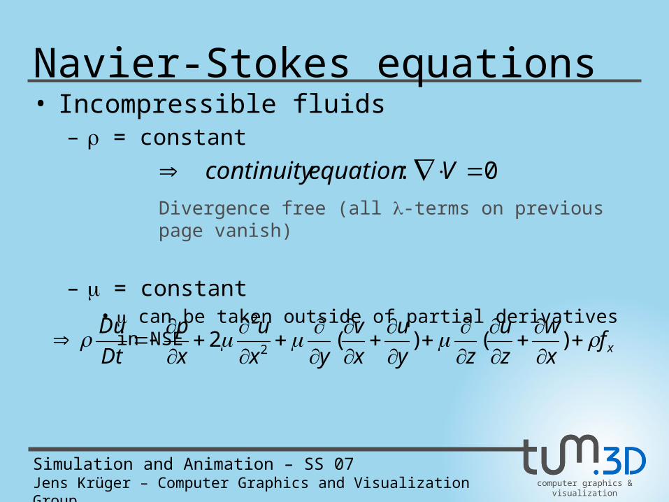
Navier-Stokes equations• Incompressible fluids

– = constant

– = constant• can be taken outside of partial derivatives in NSE

0: Vequationcontinuity

Divergence free (all -terms on previous page vanish)

xfx

w

z

u

zy

u

x

v

yx

u

x

p

Dt

Du

)()(22

2



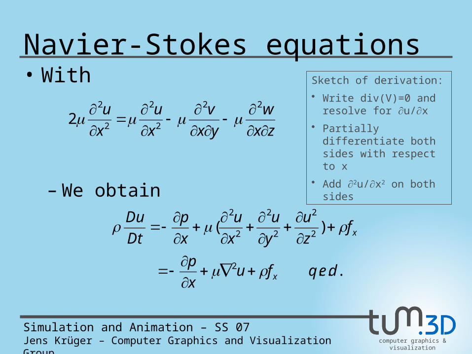
Navier-Stokes equations• With

– We obtain

zx

w

yx

v

x

u

x

u

22

2

2

2

2

2

...

)(

2

2

2

2

2

2

2

deqfux

p

fz

u

y

u

x

u

x

p

Dt

Du

x

x

Sketch of derivation:

• Write div(V)=0 and resolve for u/x

• Partially differentiate both sides with respect to x

• Add 2u/x2 on both sides



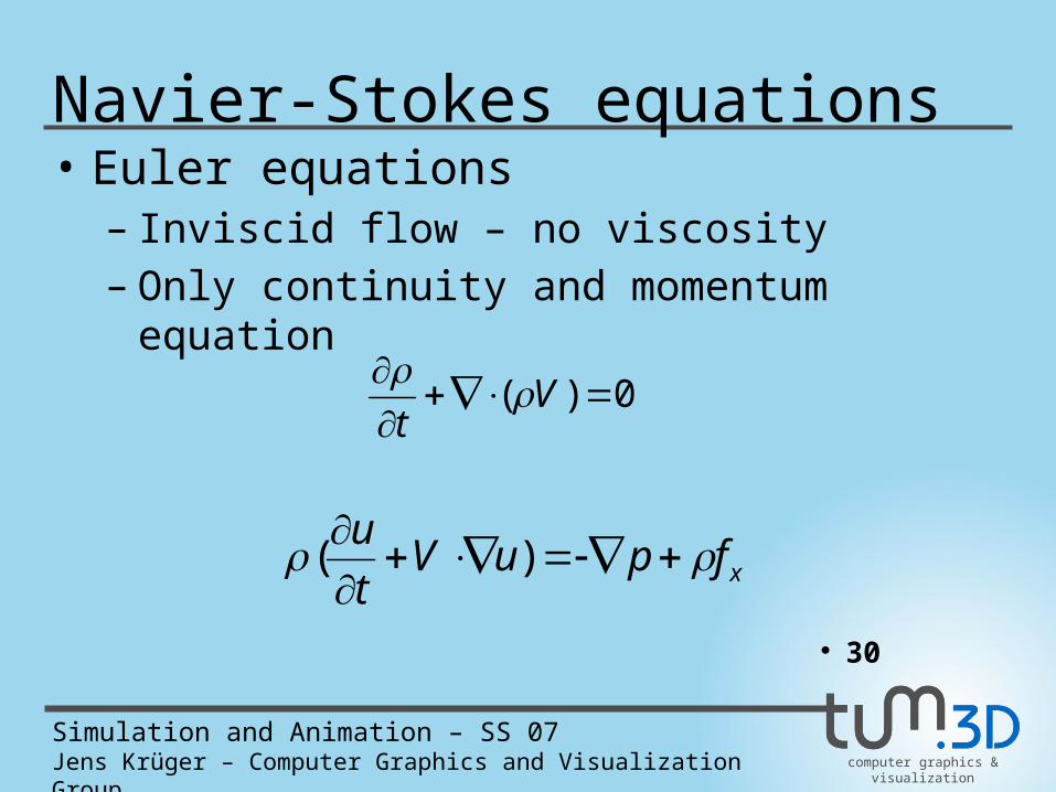
Navier-Stokes equations• Euler equations

– Inviscid flow – no viscosity– Only continuity and momentum equation

• 30

xfpuVt

u

)(

0)(

Vt



• Solution methods for governing equations– Governing equations have been derived independent of flow

situation, e.g. flow around a car or inside a tube– Boundary (and initial) conditions determine specific flow

case• Determine geometry of boundaries and behavior of flow at

boundaries– Different kinds of boundary conditions exist– Hold at any time during simulation

• Lead to different solutions of the governing equations– Exact solution exists for specific conditions

• Initial conditions specify state to start with

CFD – Computational Fluid Dynamics



• Solution methods of partial differential equations– Analytical solutions

• Lead to closed-form epressions of dependent variables• Continuously describe their variation

– Numerical solutions• Based on discretization of the domain• Replace PDEs and closed form expression by approximate

algebraic expressions– Partial derivatives become difference quotients – Involves only values at finite number of discrete points in the

domain

• Solve for values at given grid points




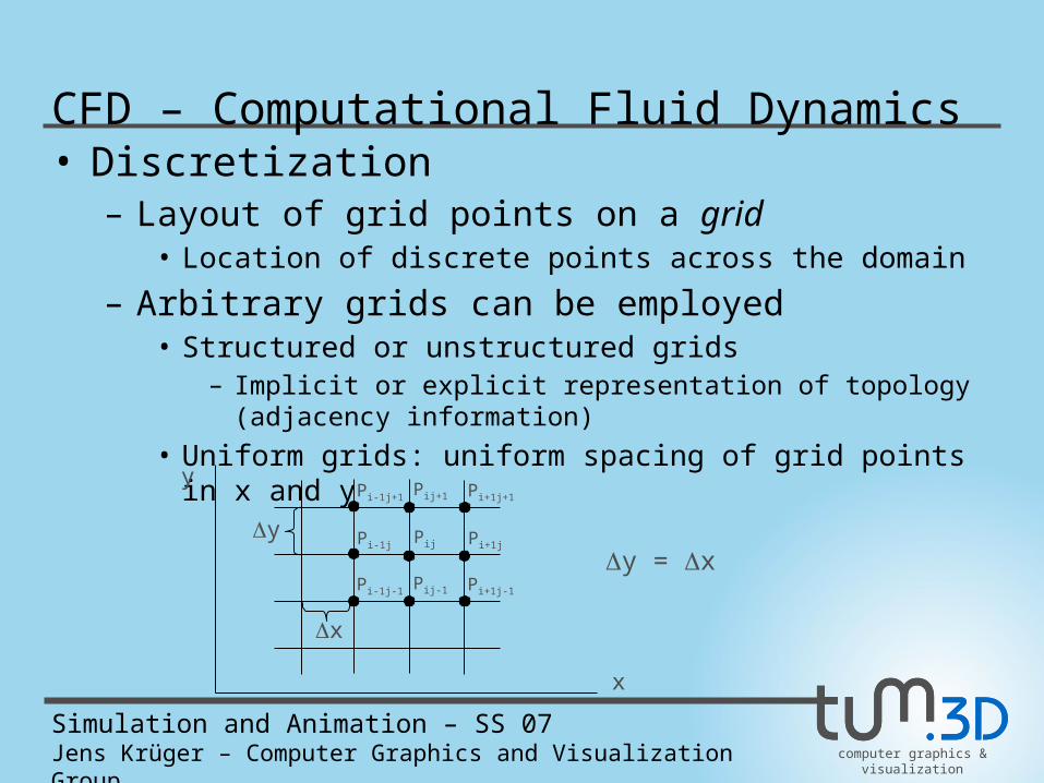
• Discretization – Layout of grid points on a grid

• Location of discrete points across the domain

– Arbitrary grids can be employed• Structured or unstructured grids

– Implicit or explicit representation of topology (adjacency information)• Uniform grids: uniform spacing of grid points in x and y

y

x

x

y Pij

Pij+1

Pij-1

Pi+1j

Pi+1j+1

Pi+1j-1

Pi-1j

Pi-1j+1

Pi-1j-1

y = x




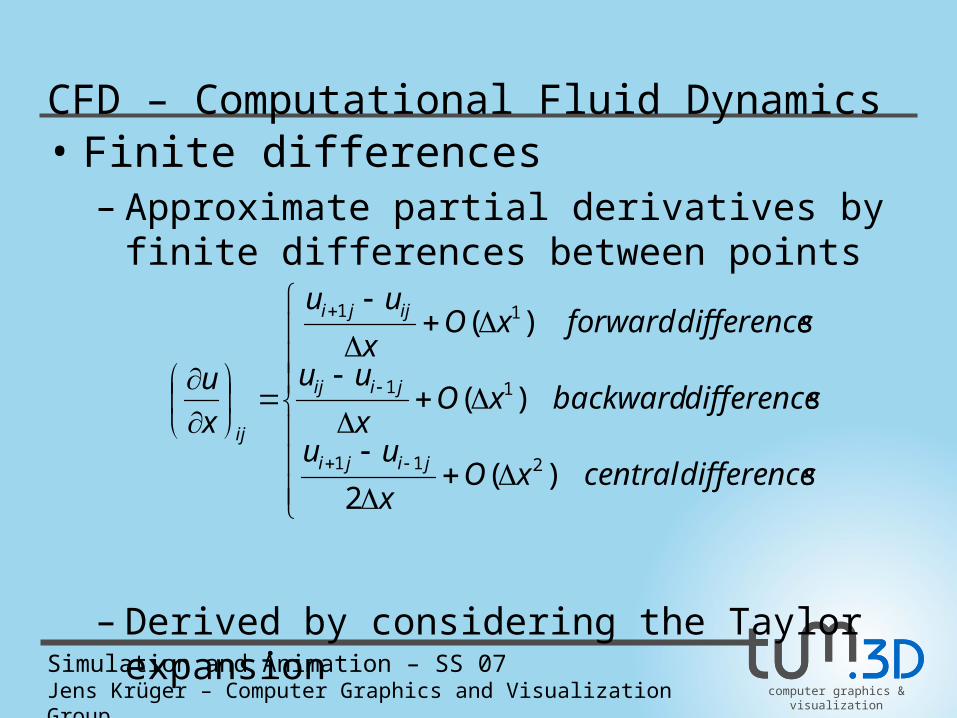
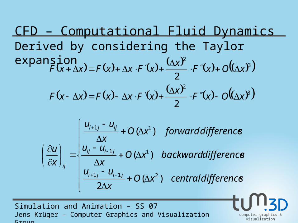
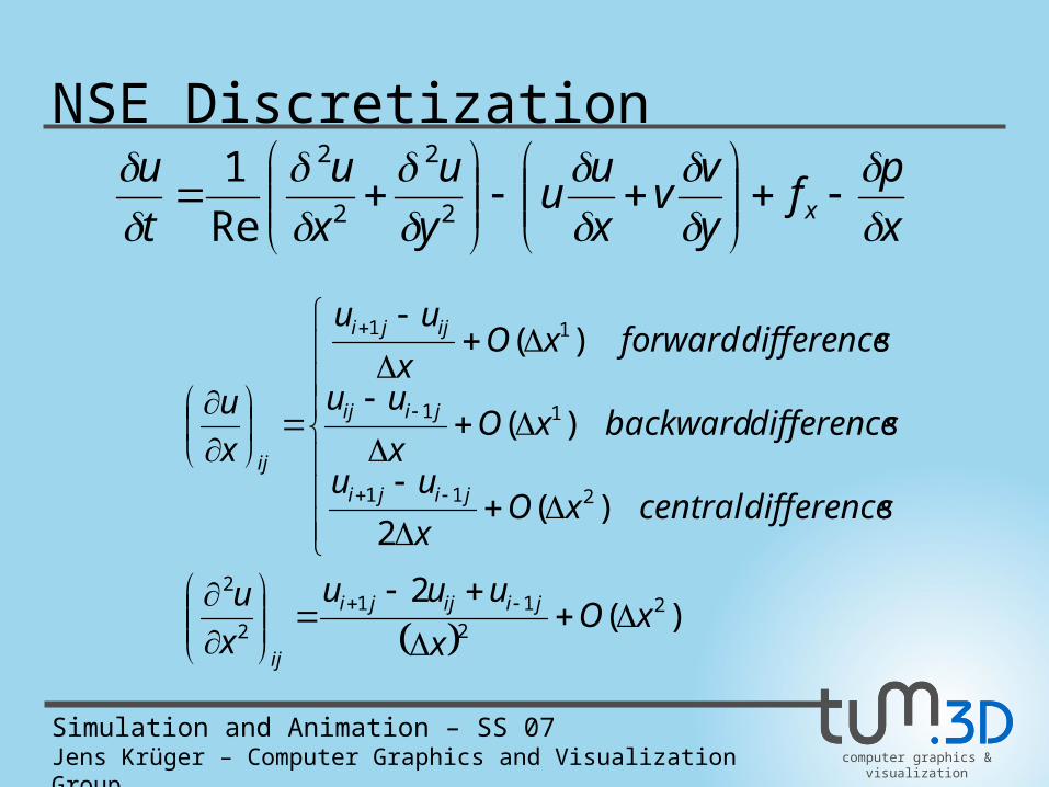
• Finite differences– Approximate partial derivatives by finite differences

between points

– Derived by considering the Taylor expansion

sdifferencecentralxOx

uu

sdifferencebackwardxOx

uu

sdifferenceforwardxOx

uu

x

u

jiji

jiij

ijji

ij

)(2

)(

)(

211

11

11




Derived by considering the Taylor expansion

32

32

2

2

xOxFx

xFxxFxxF

xOxFx

xFxxFxxF



uu


uu


uu

x

u

jiji

jiij

ijji

ij

)(2

)(

)(

211

11

11



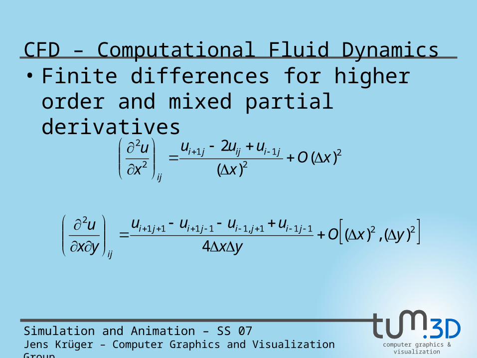
• Finite differences for higher order and mixed partial derivatives

22

11

2

2

)()(

2xO

x

uuu

x

u jiijji

ij

22111,111112

)(,)(4

yxOyx

uuuu

yx

u jijijiji

ij




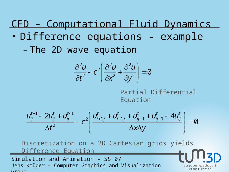
• Difference equations - example– The 2D wave equation

02

2

2

22

2

2

y

u

x

uc

t

u

042 11112

2

11

yx

uuuuuc

t

uuu tij

tij

tij

tji

tji

tij

tij

tij

Partial Differential Equation

Discretization on a 2D Cartesian grids yields Difference Equation




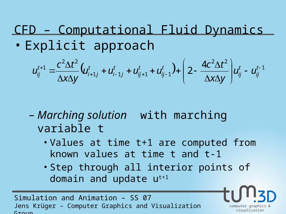
• Explicit approach

– Marching solution with marching variable t• Values at time t+1 are computed from known values at

time t and t-1• Step through all interior points of domain and update ut+1

122

1111

221 4

2

tij

tij

tij

tij

tji

tji

tij uu

yx

tcuuuu

yx

tcu




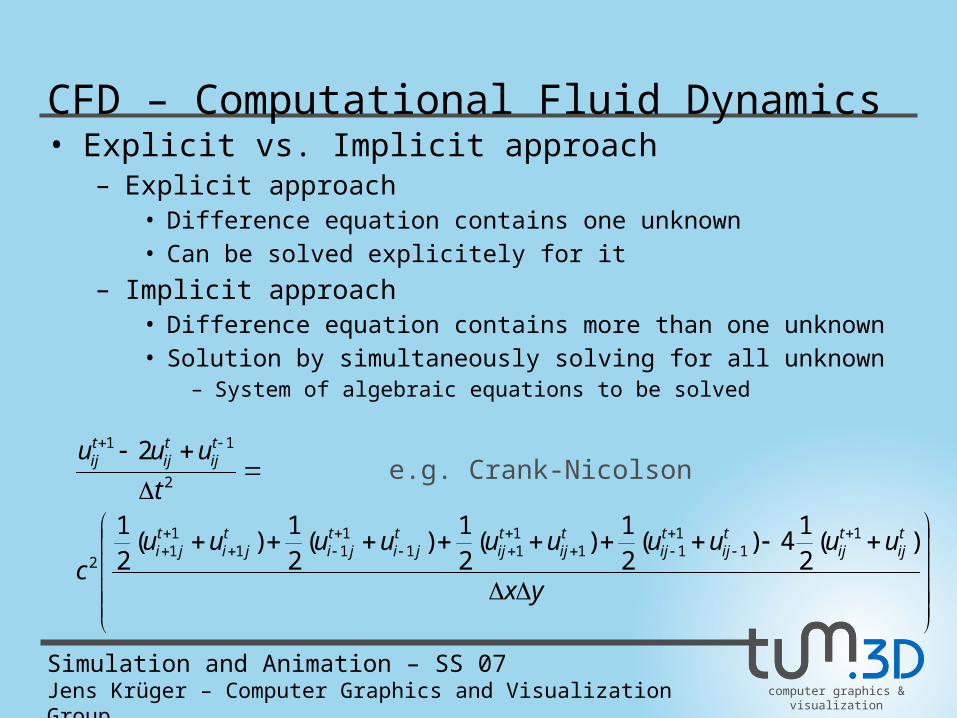
• Explicit vs. Implicit approach– Explicit approach

• Difference equation contains one unknown• Can be solved explicitely for it

– Implicit approach• Difference equation contains more than one unknown• Solution by simultaneously solving for all unknown

– System of algebraic equations to be solved

yx

uuuuuuuuuuc

t

uuu

tij

tij

tij

tij

tij

tij

tji

tji

tji

tji

tij

tij

tij

)(21

4)(21

)(21

)(21

)(21

2

11

111

111

111

11

2

2

11

e.g. Crank-Nicolson




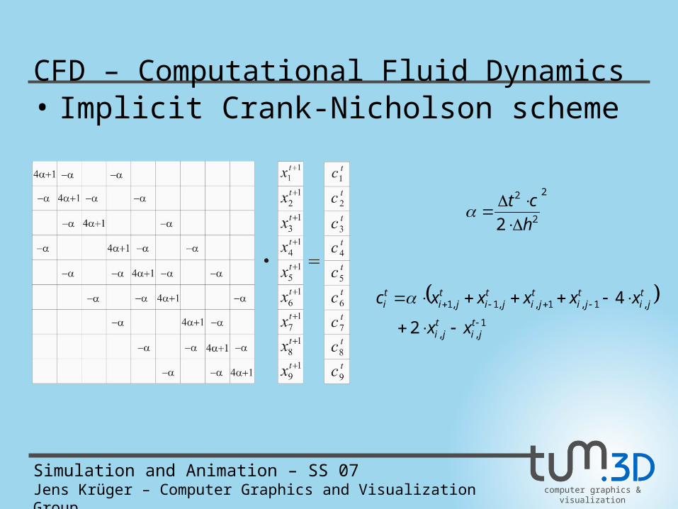
• Implicit Crank-Nicholson scheme

1

,,

,1,1,,1,1

2

4

tji

tji

tji

tji

tji

tji

tji

ti

xx

xxxxxc

2

2

2

2 h

ct




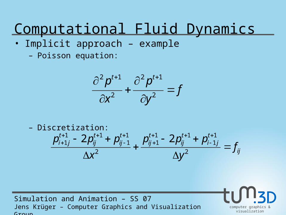
• Implicit approach – example– Poisson equation:

– Discretization:

fy

p

x

p tt

2

12

2

12

ij

tji

tij

tij

tij

tij

tji f

y

ppp

x

ppp

2

11

111

2

11

111 22

Computational Fluid Dynamics



0)(

Re

1Re

1

2

2

Vdiv

y

pfvVv

t

vx

pfuVu

t

u

y

x

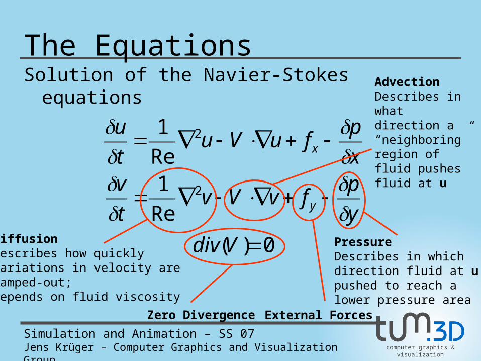
The EquationsSolution of the Navier-Stokes equations

DiffusionDescribes how quickly variations in velocity are damped-out; depends on fluid viscosity

AdvectionDescribes in what direction a “neighboring” region of fluid pushes fluid at u

External Forces

PressureDescribes in which direction fluid at u is pushed to reach a lower pressure area

Zero Divergence



NSE Discretization

x

pf

y

vv

x

uu

y

u

x

u

t

ux

2

2

2

2

Re

1

)(

2

)(2

)(

)(

22

11

2

2

211

11

11

xOx

uuu

x

u


uu


uu


uu

x

u

jiijji

ij

jiji

jiij

ijji

ij



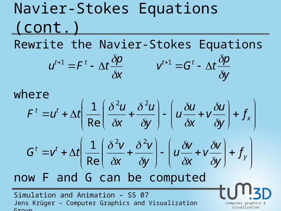
Navier-Stokes Equations (cont.)Rewrite the Navier-Stokes Equations

where

now F and G can be computed

y

ptGv

x

ptFu tttt

11

ytt

xtt

fy

vv

x

vu

y

v

x

vtvG

fy

uv

x

uu

y

u

x

utuF

22

22

Re

1

Re

1



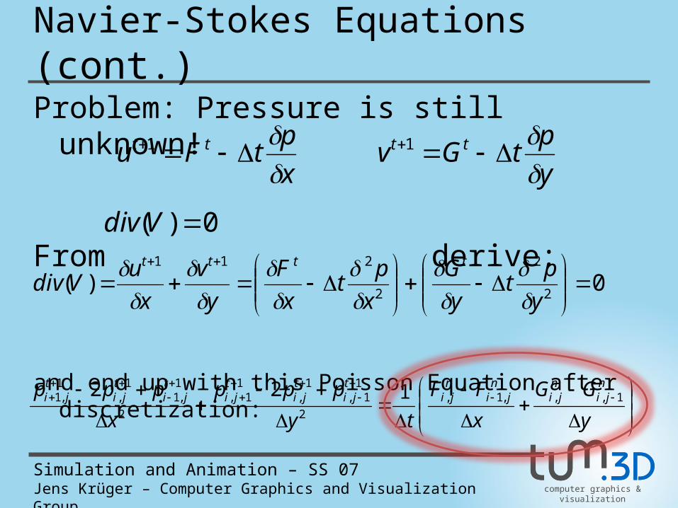
Navier-Stokes Equations (cont.)Problem: Pressure is still unknown!

From derive:

and end up with this Poisson Equation after discretization:

y

ptGv

x

ptFu tttt

11

0)( Vdiv

0)(2

2

2

211

y

pt

y

G

x

pt

x

F

y

v

x

uVdiv

tttt

y

GG

x

FF

ty

ppp

x

ppp nji

nji

nji

nji

tji

tji

tji

tji

tji

tji 1,,,1,

2

11,

1,

11,

2

1,1

1,

1,1 122



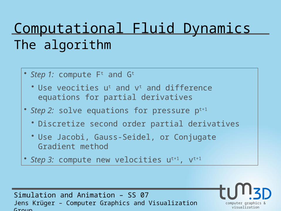
The algorithm

• Step 1: compute Ft and Gt

• Use veocities ut and vt and difference equations for partial derivatives

• Step 2: solve equations for pressure pt+1

• Discretize second order partial derivatives

• Use Jacobi, Gauss-Seidel, or Conjugate Gradient method

• Step 3: compute new velocities ut+1, vt+1

Computational Fluid Dynamics



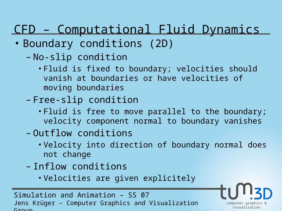
• Boundary conditions (2D)– No-slip condition

• Fluid is fixed to boundary; velocities should vanish at boundaries or have velocities of moving boundaries

– Free-slip condition• Fluid is free to move parallel to the boundary; velocity

component normal to boundary vanishes

– Outflow conditions• Velocity into direction of boundary normal does not change

– Inflow conditions• Velocities are given explicitely




Demo

Documents

Computer graphics & visualization Fluids. computer graphics & visualization Simulation and Animation – SS 07 Jens Krüger – Computer Graphics and Visualization