Embed Size (px)
Citation preview
IEEE TRANSACTIONS ON CONTROL SYSTEMS TECHNOLOGY, Vol 11, No 5, 2003, pp.612-628
Feedback Controller Design for aSpatially-Distributed System: The Paper Machine
ProblemG.E. Stewart, Member, IEEE, D.M. Gorinevsky, Senior Member, IEEE, and G.A. Dumont, Fellow, IEEE
Abstract— This article reports on the development and imple-mentation of an algorithm for the design of spatially-distributedfeedback controllers for the wide variety of physical processesthat are included in cross-directional control of industrial papermachines. The spatial and temporal structure of this class ofprocess models is exploited in the use of the two-dimensionalfrequency domain for analysis and two-dimensional loop shapingdesign of feedback controllers. This algorithm forms the basis of asoftware tool that has recently been implemented in a commercialproduct and its use is illustrated for tuning CD controllerson two different industrial paper machines. The first exampledescribes the use of the tool in stabilizing an unstable closed-loop system by retuning the distributed controller. The secondpaper machine example exposes an underperforming controller.Subsequent retuning of the controller resulted in a dramaticperformance improvement.
Index Terms— Distributed control, Industrial control, Mul-tidimensional systems, Controller tuning, Frequency domainsynthesis, Distributed parameter systems.
I. INTRODUCTION
THIS paper reports on results in the development ofalgorithms and their implementation in a software tool for
the design of a feedback controller of an industrial spatially-distributed system. The papermaking process employs largearrays of actuators spread across a continuously moving webto control the cross-directional (CD) profiles of the paperproperties as measured by a scanning gauge downstream fromthe actuators. A CD control system calculates actuator movesto maintain the measured CD profiles of paper propertieson target. Papermaking is an important multi-billion dollarindustry – in North America and worldwide – and CD controlon paper machines is arguably the most established industrialapplication of spatially-distributed control.
CD control has been long recognized as an interesting andchallenging problem by the control systems community andthere have been many papers published studying design ofvarious CD control algorithms. The CD control approachesstudied in the literature include robust control design [1], [2],[3], [4], [5], various subspace and dimensionality reductionmethods [6], [7], [8], minimum variance control [9], [8],as well as two-dimensional control methods [10]. However,
Department of Electrical and Computer Engineering, University ofBritish Columbia, 2356 Main Mall, Vancouver, B.C., Canada V6T [email protected]
Honeywell Industry Solutions, 500 Brooksbank Avenue, North Vancouver,B.C., Canada V7J 3S4.
Honeywell Laboratories, One Results Way, Cupertino, CA, USA 95014.
most of the control laws proposed and studied in the abovementioned papers, have not been used in industry, except forsome short-term trials.
Online optimization methods such as model predictive con-trol (MPC) are an attractive possibility due to their abilityto address hard physical constraints on the actuators. Thelimitation of these techniques has traditionally been due tothe enormous online computational load and their sensitivityto model uncertainty. However advances in computing powercoupled with theoretical work in model reduction and ro-bustness (for example [5], [11]) are beginning to make suchtechniques tractable. Industrial examples of optimization basedCD controllers may be found in [12], [9], [13].
Industrial CD control systems have been installed in thefield for more than two decades and their algorithms evolvedover time to attain an acceptable tradeoff between the achiev-able closed-loop performance (which requires sophisticatedalgorithms) and the ease of support and maintenance (whichrequires simple, easily understandable algorithms for tuning).In the paper industry, simplicity of use is especially importantbecause support and maintenance are typically performed bytechnician-level personnel. In addition, acceptance of newalgorithms (even if they are simple) is usually slow, becausethere is a large existing base of installed CD control systems.These are typically maintained and supported by their re-spective vendors. In many CD control installations significantperformance improvements can be achieved for an existingcontroller by implementing a better tuning of the controlloop. The tuning problem is to select optimal values for thefree parameters within the fixed control algorithms, and CDcontroller tuning is the main topic of this paper. There islittle literature on this topic, the majority of which consistsof conference papers by the authors of the present paper[14], [15]. This paper is meant as a first archival publicationcovering this gap.
CD control tuning has to take into account the usual issuesof stability, robustness, and disturbance rejection performance.In addition to that, there are issues of spatial stability andperformance of the control that are specific for the CD processcontrol. Closed-loop spatial instability of CD control might becaused by poor controllability of the process at high spatialfrequencies. The spatial instability manifested as a picket fencepattern of the actuator setpoints (actuator picketing) is a wellknown and often encountered problem in industrial CD controlinstallations and indicates a controller that has been designedsuch that it is chasing uncontrollable components of the error
IEEE TRANSACTIONS ON CONTROL SYSTEMS TECHNOLOGY 2003 2
signal [16].This paper presents the architecture of a typical industrial
CD control system. The tuning algorithms are herein de-veloped for such an architecture. Interestingly enough, CDcontrol systems independently developed by different vendorshave many similarities in the structure of the control law,despite the claimed use of various proprietary algorithms forsignal processing and control. This is because many existingCD control systems have evolved over time starting fromthe simplest algorithms and adding controller enhancementas the performance problems with some of the deployedcontrollers became apparent. The simplest algorithm for CDcontrol is mapped or zone-by-zone control where the measuredhigh-resolution profile error is mapped to yield errors foreach actuators. The simple mapped CD control does notwork well where the CD response of neighboring actuatorsoverlap significantly. This was recognized by the industryand overcome by introducing error decoupling and actuatorprofile smoothing terms in the control law. Such an industrialcontroller structure is considered in this paper.
The design, implementation, and field testing of the CDcontrol tuner described herein was enabled by a use of theautomated identification tool described in [17], [18], [19], [20].The identification provides a CD process model required forthe control analysis and tuning. In what follows, the structureof the accepted CD process model and the industrial CDcontrol law structure are discussed in more detail.
Overall, the main contributions of this paper include thefollowing: (i) a thorough study of an industrial CD controlengineering problem; (ii) an application of a novel two-dimensional loop shaping design procedure to CD controllertuning; (iii) construction of an industrial software tool for theanalysis and tuning of the feedback controller; (iv) presentationof typical industrial results.
A. Notation
This article makes extensive use of banded, symmetricmatrices – Toeplitz and circulant. A band-diagonal symmetricToeplitz matrix of size nn with q < n=2 degrees of freedoma = [a1; : : : ; aq ]
T will be denoted by,
A = T (a; n)
:=
266666666666666666666664
a1 a2 aq 0 0
a2 a1 a2 aq 0. . .
. . .. . .
...... a2 a1 a2
... aq. . .
. . .. . .
...
aq a2 a1 a2. . .
. . .. . .
. . ....
0 aq a2. . .
. . .. . . aq 0
...... 0 aq
. . .. . .
. . . a2. . . aq 0
.... . .
. . .. . .
. . . a2 a1 a2. . . aq
.... . .
. . .. . . aq
. . . a2 a1 a2...
.... . .
. . .. . . 0 aq a2 a1 a2
0 0 aq a2 a1
377777777777777777777775
| z n n (1)
The related symmetric circulant matrix [21], [22] will bedenoted by,
A = C(a; n)
:=
266666666666666666666664
a1 a2 aq 0 0 aq a2
a2 a1 a2 aq 0. . .
. . .. . .
...... a2 a1 a2
... aq. . .
. . .. . . aq
aq a2 a1 a2. . .
. . .. . .
. . . 0
0 aq a2. . .
. . .. . . aq 0
...... 0 aq
. . .. . .
. . . a2. . . aq 0
0. . .
. . .. . .
. . . a2 a1 a2. . . aq
aq. . .
. . .. . . aq
. . . a2 a1 a2...
.... . .
. . .. . . 0 aq a2 a1 a2
a2 aq 0 0 aq a2 a1
377777777777777777777775
| z n n (2)
Throughout this article, variable with a ‘hat’ such as A willbe used to represent circulant matrices and their associatedeigenvalues.
Note that the two matrices T (a; n) in (1) and C(a; n) in (2)are the same except for the upper right and lower left corners.This fact will be revisited in Section IV.
II. PROBLEM STATEMENT
A. Industrial Cross-Directional Control Processes
An overview of a paper machine showing relative positionsof the various actuator arrays and scanning sensor is shown inFigure 1. The wet pulp slurry enters the machine at the left ofFigure 1 where it is distributed over a wide area and forcedthrough a gap governed by the slice lip where it is extruded onto a moving wire screen. The remainder of the paper machinefirst drains then dries the majority of the water from the pulpand a formed sheet of paper is rolled up as illustrated at theright of Figure 1.
The three main properties of interest are weight, moisture,and caliper. The control tuning results shown in Section VI arefor two different types of weight control problems - one usinga slice lip actuator array and the other a consistency profilingactuator array, which will be described shortly.
The weight per unit area of a sheet of paper, expressedin grams per square meter (gsm) or in pounds per ream isan important factor in the quality of the finished product.Deviations in the paper sheet’s weight from its target willaffect most other properties [23]. The desired weight targetsfor papermaking cover a wide range. A sheet of newsprint hasa target weight of about 45gsm, a paperback book cover mayhave a weight of about 300gsm, and cardboard may weigh450gsm.
CD control of the weight of a paper sheet is accomplishedby actuators at the headbox (left side in Figure 1). The functionof weight control actuators is to achieve an even distributionof the pulp fibres across the width of the wire belt, despite
IEEE TRANSACTIONS ON CONTROL SYSTEMS TECHNOLOGY 2003 3
FRQVLVWHQF\SURILOLQJ
ZLUHVFUHHQ
UHZHWVKRZHU
VOLFHOLS VWHDPER[VFDQQLQJVHQVRUV
LQGXFWLRQKHDWLQJ
Fig. 1. Wide view of the paper machine showing typical positions of the various actuator arrays and scanning sensor(s). (Artwork courtesy of HoneywellIndustry Solutions.)
changing pulp properties. Since the weight control actuatorsare located the furthest upstream, the dynamics of weightcontrol often require the consideration of a significant deadtime component, as the paper sheet must travel through theentire machine before reaching the scanning sensor.
Due to the nature of the raw material, the pulp stockcharacteristics change over time. The consistency and drainageproperties of the delivered stock are kept as constant aspossible by the approach system, but variability inevitablyoccurs. In addition, the flow of the pulp stock through theheadbox and on the wire belt can distribute the wood fibresunevenly in the cross-direction. Basis weight profile controlis important not only for paper strength reasons, but also dueto the fact that a poor quality weight profile will propagatedownstream and appear as disturbances in both the moistureand caliper profiles. The control of weight profiles with slicelip actuators and consistency profiling actuators is describedin Section VI.
The moisture content of a sheet of paper is a very importantfactor in determining paper strength [23]. Typical moisturecontent targets are 5–9% of the total weight of the paper sheet.Overdrying a paper sheet will reduce its strength as the fibresare damaged. An excessively variable moisture profile leads toa variable temperature profile and thus increases the demandon the caliper profiling actuators.
The dewatering and drying of the paper sheet as it passesthrough the paper machine is very complex and is affectedby many factors. The fibre slurry exiting the headbox isapproximately 0.5% fibres and 99.5% water. The paper whichis wound up on the reel is about 95% fibres and 5% water.The goal of feedback CD control of moisture is to performthe fine control and level a variable moisture profile.
The caliper of a sheet of paper is controlled by feeding thepaper sheet through rotating rollers, known as the calendarstack. The pressure that the rolls exert on the paper sheet maybe adjusted by locally heating (cooling) one of the rollers. Asthe temperature of the roller increases (decreases), its diameteralso increases (decreases) due to thermal expansion, and thus
the pressure on the paper sheet increases (decreases), leadingto a decrease (increase) in the paper caliper [24].
Early CD caliper control was implemented through the useof hot and cold air showers on the roller. Modern calipercontrol is much more efficient and uses induction heatingactuators. A high frequency alternating current is used togenerate an oscillating magnetic field at the roller surface. Theresulting eddy currents near the surface of the roller cause thetemperature of the roller to rise, and a local increase in rollerdiameter with subsequent pressure on the paper sheet.
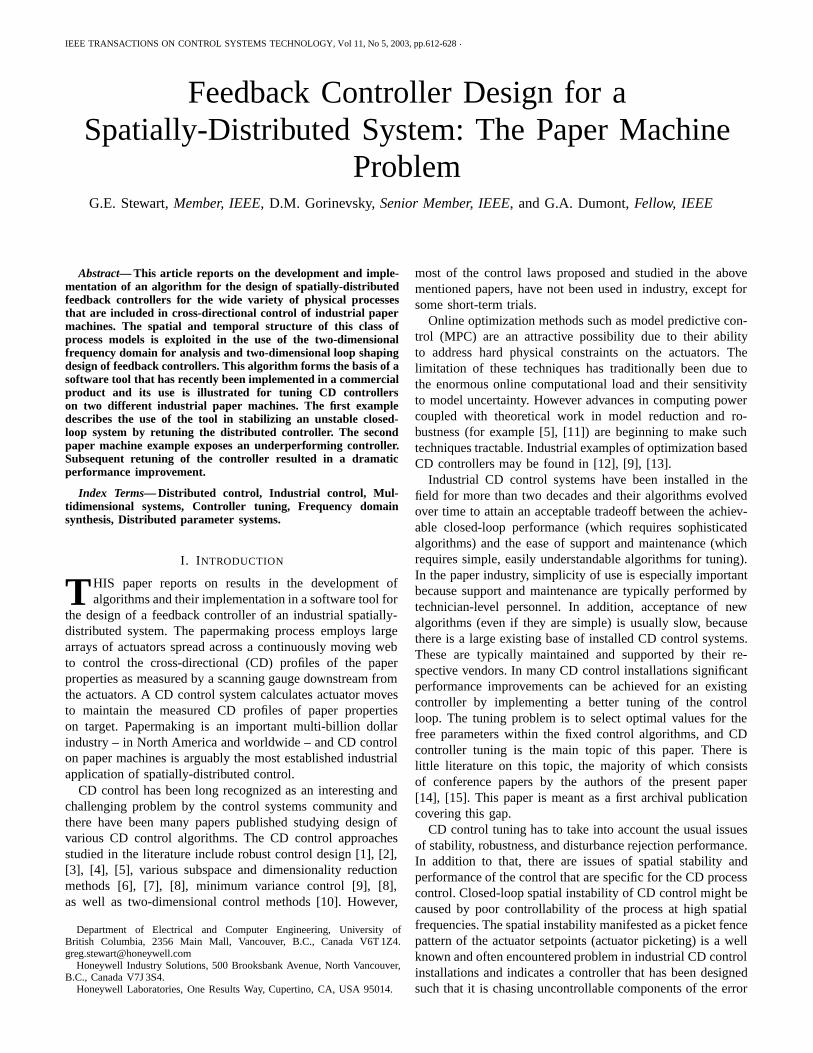
B. Process Model
The high-level structure of a typical industrial CD controlsystem is illustrated in Figure 2. This structure is discussedin more details in the next section. It is important to notethat the computations in a CD control system are organizedin two parts. The upper part of the diagram shows controllercomputations that are performed at the spatial resolution ofthe actuator profile. Such profiles have 30–300 elements,corresponding to the number of the actuators.
PaperMachine
ActuatorsScanningGauge
SpatialFiltering
DynamicalCompensator
Actuator ProfileSmoothing
Measurement SystemSignal Processing
Low-levelSafety Logic
targetprofile mapped profile
Fig. 2. The flow of information for an industrial cross-directional controlsystem.
The lower part of Figure 2 illustrates the operations involvedin processing the signal obtained from the scanning sensor ata much higher spatial resolution with up to 2000 elements.As illustrated in Figure 1, this sensor is mounted on a fixedframe and is scanning back and forth across the paper sheet ata rate of 15–45 seconds per crossing. Because the paper sheetis moving, the scanner actually traces out a zig-zag path on
IEEE TRANSACTIONS ON CONTROL SYSTEMS TECHNOLOGY 2003 4
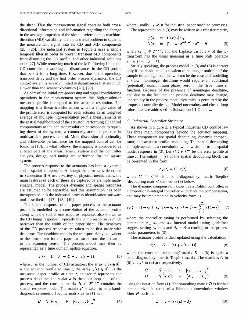
the sheet. Thus the measurement signal contains both cross-directional information and information regarding the changein the average properties of the sheet – referred to as machine-direction (MD) variability. It is not a trivial problem to separatethe measurement signal into its CD and MD components[25], [26]. The industrial system in Figure 2 uses a simpletemporal filter in order to prevent transient MD componentsfrom distorting the CD profile, and other industrial solutionsexist [27]. While removing much of the MD, filtering limits theCD controller to working on disturbances in the CD profilethat persist for a long time. However, due to the open-looptransport delay and the first order process dynamics, the CDcontrol system is already limited to disturbances that are muchslower than the scanner dynamics [28], [29].
As part of the initial pre-processing and signal conditioningoperations in the measurement system this high-resolutionmeasured profile is mapped to the actuator resolution. Themapping is a linear transformation where a single value ofthe profile error is computed for each actuator as an weightedaverage of multiple high-resolution profile measurements inthe spatial neighborhood of the actuator. Performing all controlcomputations at the actuator resolution corresponds to squar-ing down of the system, a commonly accepted practice inmultivariable process control. More discussion of optimalityand achievable performance for the mapped control can befound in [18]. In what follows, the mapping is considered asa fixed part of the measurement system and the controlleranalysis, design, and tuning are performed for the squaresystem.
The process response to the actuators has both a dynamicand a spatial component. Although the processes describedin Subsection II-A use a variety of physical mechanisms, themain features of each of these are captured by a simple math-ematical model. The process dynamic and spatial responsesare assumed to be separable, and this assumption has beenincorporated into the industrial process identification softwaretool described in [17], [18], [19].
The spatial response of the paper process to the actuatorprofile is modelled by a convolution of the actuator profilealong with the spatial unit impulse response, also known asthe CD bump response. Typically the bump response is muchnarrower than the width of the paper sheet. The dynamicsof the CD process response are taken to be first order withdeadtime. The deadtime models the transport delay equivalentto the time taken for the paper to travel from the actuatorsto the scanning sensor. The process model may then berepresented as a time domain update equation,
y(t) = B u(t d) + a y(t 1); (3)
where n is the number of CD actuators, the array u(t) 2 <n
is the actuator profile at time t, the array y(t) 2 <n is themeasured paper profile at time t, integer d represents theprocess deadtime, the scalar a is the open-loop pole of theprocess, and the constant matrix B 2 <nn contains thespatial response model. The matrix B is taken to be a band-diagonal, symmetric Toeplitz matrix as in (1) with,
B = T (b; n); b = [b1; : : : ; bnb ]T (4)
where usually nb n for industrial paper machine processes.The representation in (3) may be written as a transfer matrix,
y(z) = G(z)u(z);
G(z) = [1 a z1]1 zd B (5)
where G(z) 2 Cnn, and the Laplace variable z of the Z-transform has the usual meaning as a time shift operatorz1u(t) = u(t 1).
Strictly speaking, the process model in (3) and (5) is correctonly if the deadtime is equivalent to an integer multiple of thesample time. In general this will not be the case and modellinga known noninteger deadtime would require an additional(potentially nonminimum phase) zero in the ‘true’ transferfunction. Because of the presence of noninteger deadtime,and due to the fact that the process deadtime may change,uncertainty in the process model dynamics is permitted by theproposed controller design. Model uncertainty and closed-looprobustness are addressed in Subsection III-C below.
C. Industrial Controller Structure
As shown in Figure 2, a typical industrial CD control lawhas three main components beyond the actuator mapping.These components are spatial decoupling, dynamic compen-sator, and actuator profile smoothing. The spatial decouplingis implemented as a convolution window similar to the spatialmodel response in (3). Let e(t) 2 <n be the error profile attime t. The output ew(t) of the spatial decoupling block canbe presented in the form
ew(t) = C e(t); (6)
where C 2 <nn is a band-diagonal symmetric Toeplitz‘decoupling matrix’ defined in (9) below.
The dynamic compensator, known as a Dahlin controller, isa proportional-integral controller with deadtime compensation,and may be implemented in velocity form as
v(t) = (1 c)
"ew(t) ac ew(t 1)
dc1Xi=1
v(t i)
#(7)
where the controller tuning is performed by selecting theparameters c, ac, and dc. Internal model tuning guidelinessuggest setting ac = a and dc = d according to the processmodel parameters in (3).
The actuator profile is then updated using the calculation,
u(t) = D [v(t) + u(t 1)]; (8)
where the constant ‘smoothing’ matrix D in (8) is again aband-diagonal, symmetric Toeplitz matrix. The matrices C in(6) and D in (8) are respectively,
C = T (c; n); c = [c1; : : : ; cnc ]T
D = T ( d; n); d = [d1; : : : ; dnd ]T (9)
using the notation from (1). The smoothing matrix D is furtherparameterized in terms of a Blackman convolution windowfilter H such that
D = I + (H I) (10)
IEEE TRANSACTIONS ON CONTROL SYSTEMS TECHNOLOGY 2003 5
where 0 < 1 and nd defines the width of D in (8), (10),with H being a symmetric Toeplitz matrix,
H = T (h; n); h = [h1; : : : ; hnd ]T (11)
where the elements of h are defined by a lowpass Blackmanwindow of order nd normalized such that h1 + 2 h2 + : : :+2 hnd = 1. Consider for example nd = 3 in (11), then[h1; h2; h3] = [0:3968; 0:2500; 0:0516], so that h3+h2+h1+h2 + h3 = 1.
Note that the actuator profile smoothing operation (8) isresponsible for providing the integrator in the control loop.Typically the loop is tuned with 0 such that D I in(8) in order to preserve the closed-loop performance at lowfrequencies !. However, we will see in Section V that D 6= Iis necessary to guarantee stable closed-loop operation withnonzero model uncertainty.
The feedback controller, (6)–(8) can be written as a transfermatrix,
u(z) = K(z)e(z);
K(z) = [I D z1]1D c(z) C (12)
where the constant matrices C and D are defined in (6) and(8)–(11) respectively. The scalar transfer function,
c(z) =(1 c)[1 acz
1]
1 + (1 c)Pdc1
i=1 zi(13)
represents the Z-transform of the Dahlin controller in (7).
III. CLOSED-LOOP REQUIREMENTS
The following specifications must be satisfied for an accept-able industrial control design.
A. Internal Stability
All processes in question are open-loop stable (0 < a < 1in (5)). The feedback controller itself may be marginally stable(0 < c < 1 and jeig(D)j 1 in (12)), then the requirementof internal stability is equivalent to specifying that the closed-loop transfer matrix,
K(z) (I +G(z)K(z))1 (14)
is stable (analytic for all jzj 1 and z 2 C) with K(z) in(12) and G(z) in (5).
B. Performance
Cross-directional control is largely a regulation problemand performance is specified by the effect of the outputdisturbance dy on the error profile e = r y. Expand-ing the specification frequency-by-frequency with d y(!)
T =[dy1e
i(!t+1); : : : ; dynei(!t+n)] we write,
kek2kdyk2
<1
p; 8 dy 2 l (15)
where p 1, the norm is defined kdy(!)k2 :=pdy(!)Hdy(!) (the superscript H denotes the conjugate
transpose). In an ideal design, the set l would contain allsignificant disturbances in the system. However, in practice a
performance specification such as (15) can only be enforcedfor controllable disturbances1, typically at low temporal fre-quencies ! (see for example [30], [31]). The form of theperformance specification (15) allows for additional flexibilityaccording to the directionality of the disturbance dy. Thenecessity of this was the central issue of [32] and will bedemonstrated in Section V below.
C. Robust Stability Margin
The parameters of the process model G(z) in (5) areidentified from input/output process data, and uncertainty inthe model is unavoidable. CD processes are somewhat unusualcontrol systems in that, due to the ill-conditioning, there is asign uncertainty of the steady-state gain (! = 0) in certaininput directions of the process [32], [33], [1]. This form ofmodel uncertainty may be captured with an additive matrixperturbation,
Gp(z) = G(z) + ÆG(z) (16)
Then designing the controller K(z) such that the closed-loopis internally stable (condition (14)) and
maxdy 6=0
kuk2kdyk2
= (K[I +GK]1) <1
(17)
where () denotes the maximum singular value, provides arobust stability margin of to additive matrix perturbations.In other words, the closed-loop is robustly stable for allprocesses described by (16) with uncertainty given by a stableperturbation bounded as,
kÆG(z)k1 (18)
D. Low-Order Controller
Low-order controllers are preferred over high-order. From(7) or (13) it is evident that the temporal order of the controlleris determined by dc which typically is set equal to the processmodel dead time d in (3), (5). The spatial order of thecontroller2 is defined by the number of nonzero off-diagonalelements nc and nd respectively for the system matrices Cand D in (9). The low spatial order requirement is then toensure that
nc; nd n (19)
in (9) where n is the dimension of the matrices C;D 2 <nn.
IV. TWO-DIMENSIONAL FREQUENCY DOMAIN
A straightforward approach to the above problem requiresdealing with a multivariable feedback control system that willhave up to n = 300 inputs and outputs. However, to addressthis problem directly is difficult if not intractable. By appealing
1Sometimes a high-performance low-frequency specification such as (15)will be accompanied by a looser limit p < 1 that must be satisfied for alloutput disturbances dy with kdyk2 < 1. This is accomplished indirectlysince satisfying the robust stability condition (17) automatically satisfies (15)with p = =( + kG(z)k
1) for all such bounded dy .
2A distributed controller, implemented with a low spatial order is alterna-tively referred to as “localized control” [34], [35].
IEEE TRANSACTIONS ON CONTROL SYSTEMS TECHNOLOGY 2003 6
to the structure of the specified system, we will approach thedesign through a related problem that offers many advantages.
Section II has presented a process model and feedback con-troller that are each linear, time-invariant, and almost spatially-invariant. The convenience of the linear, time invariant (LTI)approximation is that it permits the use of the temporal fre-quency domain in the analysis and design of control systems.Recent work on linear, spatially-invariant (LSI) control sys-tems [34], [36], [37], [32], [33] has exploited the LSI propertyto a similar advantage in the spatial frequency domain. Theuse of spatially-invariant process models in cross-directionalcontrol was introduced in [4] where a thorough development ofspatial frequencies may be found. This approach has been usedsubsequently in an analogous but somewhat different mannerin [2] and more such examples may be found in [5], [38],[39].
As seen in Section II, the form of the model implies thatthe process response is the same for each actuator, exceptthat it is shifted accordingly in the cross-direction. The spatialinvariance is disrupted by the edges of the paper sheet wherethe response is truncated. The same kind of structure ispresent in the industrial CD controller as well. The effect ofsuch spatial boundary effects in distributed control systems iscurrently the subject of active research (see [40], [41]).
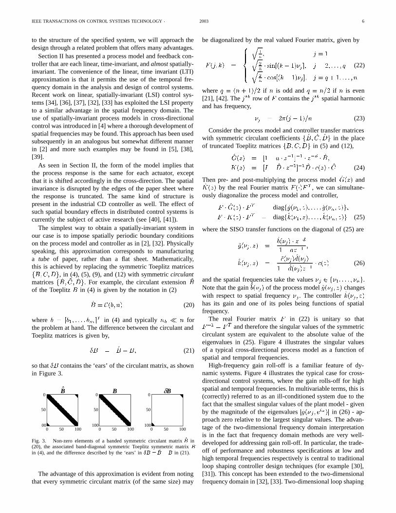
The simplest way to obtain a spatially-invariant system inour case is to impose spatially periodic boundary conditionson the process model and controller as in [2], [32]. Physicallyspeaking, this approximation corresponds to manufacturinga tube of paper, rather than a flat sheet. Mathematically,this is achieved by replacing the symmetric Toeplitz matricesfB;C;Dg, in (4), (5), (9), and (12) with symmetric circulantmatrices fB; C; Dg. For example, the circulant extension Bof the Toeplitz B in (4) is given by the notation in (2)
B = C(b; n) (20)
where b = [b1; : : : ; bnb ]T in (4) and typically nb n for
the problem at hand. The difference between the circulant andToeplitz matrices is given by,
ÆB = B B; (21)
so that ÆB contains the ‘ears’ of the circulant matrix, as shownin Figure 3.
0
50
00
0
50
100
0
50
1000 50 100 0 50 100 0 50 100
ˆ B δBB
Fig. 3. Non-zero elements of a banded symmetric circulant matrix B in(20), the associated band-diagonal symmetric Toeplitz symmetric matrix Bin (4), and the difference described by the ‘ears’ in ÆB =B B in (21).
The advantage of this approximation is evident from notingthat every symmetric circulant matrix (of the same size) may
be diagonalized by the real valued Fourier matrix, given by
F (j; k) =
8>>><>>>:
q1n; j = 1q
2n sin[(k 1)j ]; j = 2; : : : ; qq
2n cos[(k 1)j ]; j = q + 1; : : : ; n
(22)
where q = (n + 1)=2 if n is odd and q = n=2 if n is even[21], [42]. The j th row of F contains the j th spatial harmonicand has frequency,
j = 2(j 1)=n (23)
Consider the process model and controller transfer matriceswith symmetric circulant coefficients fB; C; Dg in the placeof truncated Toeplitz matrices fB;C;Dg in (5) and (12),
G(z) = [1 a z1]1 zd B;K(z) = [I D z1]1D c(z) C (24)
Then pre- and post-multiplying the process model G(z) andK(z) by the real Fourier matrix F ()F T , we can simultane-ously diagonalize the process model and controller,
F G(z) F T = diagfg(1; z); : : : ; g(n; z)g;F K(z) F T = diagfk(1; z); : : : ; k(n; z)g (25)
where the SISO transfer functions on the diagonal of (25) are
g(j ; z) =b(j) zd1 az1
;
k(j ; z) =c(j)d(j)
1 d(j)z1 c(z) (26)
and the spatial frequencies take the values j 2 f1; : : : ; ng.Note that the gain b(j) of the process model g(j ; z) changeswith respect to spatial frequency j . The controller k(j ; z)has its gain and one of its poles being functions of spatialfrequency.
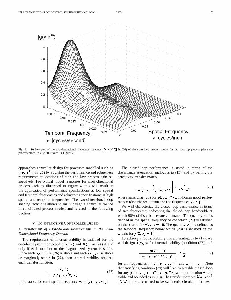
The real Fourier matrix F in (22) is unitary so thatF1 = F T and therefore the singular values of the symmetriccirculant system are equivalent to the absolute value of theeigenvalues in (25). Figure 4 illustrates the singular valuesof a typical cross-directional process model as a function ofspatial and temporal frequencies.
High-frequency gain roll-off is a familiar feature of dy-namic systems. Figure 4 illustrates the typical case for cross-directional control systems, where the gain rolls-off for highspatial and temporal frequencies. In multivariable terms, this is(correctly) referred to as an ill-conditioned system due to thefact that the smallest singular values of the plant model - givenby the magnitude of the eigenvalues jg(j ; ei!)j in (26) - ap-proach zero relative to the largest singular values. The advan-tage of the two-dimensional frequency domain interpretationis in the fact that frequency domain methods are very well-developed for addressing gain roll-off. In particular, the trade-off of performance and robustness specifications at low andhigh temporal frequencies respectively is central to traditionalloop shaping controller design techniques (for example [30],[31]). This concept has been extended to the two-dimensionalfrequency domain in [32], [33]. Two-dimensional loop shaping
IEEE TRANSACTIONS ON CONTROL SYSTEMS TECHNOLOGY 2003 7
0.0050.01
0.0150.02
0.0250.03
00.02
0.040.06
0.080.1
0
0.2
0.4
0.6
0.8
1
Spatial Frequency, ν [cycles/inch]
Temporal Frequency,
|g(ν,eiω)|
ω [cycles/second]
Fig. 4. Surface plot of the two-dimensional frequency response jg(j ; ei!)j in (26) of the open-loop process model for the slice lip process (the sameprocess model is also illustrated in Figure 7).
approaches controller design for processes modelled such asg(j ; e
i!) in (26) by applying the performance and robustnessrequirements at locations of high and low process gain re-spectively. For typical model responses for cross-directionalprocess such as illustrated in Figure 4, this will result inthe application of performance specifications at low spatialand temporal frequencies and robustness specifications at highspatial and temporal frequencies. The two-dimensional loopshaping technique allows to easily design a controller for theill-conditioned process model, and is used in the followingSection.
V. CONSTRUCTIVE CONTROLLER DESIGN
A. Restatement of Closed-Loop Requirements in the Two-Dimensional Frequency Domain
The requirement of internal stability is satisfied for thecirculant system composed of G(z) and K(z) in (24) if andonly if each member of the diagonalized system is stable.Since each g(j ; z) in (26) is stable and each k(j ; z) is stableor marginally stable in (26), then internal stability requireseach transfer function,
k(j ; z)
1 + g(j ; z)k(j ; z)(27)
to be stable for each spatial frequency j 2 f1; : : : ; ng.
The closed-loop performance is stated in terms of thedisturbance attenuation analogous to (15), and by writing thesensitivity transfer matrix 1
1 + g(j ; ei!)k(j ; ei!)
< 1
p(; !)(28)
where satisfying (28) for p(; !) 1 indicates good perfor-mance (disturbance attenuation) at frequencies f; !g.
We will characterize the closed-loop performance in termsof two frequencies indicating the closed-loop bandwidth atwhich 90% of disturbances are attenuated. The quantity 90 isdefined as the spatial frequency below which (28) is satisfiedon the -axis for p(; 0) = 10. The quantity !90 is defined asthe temporal frequency below which (28) is satisfied on the!-axis for p(0; !) = 10.
To achieve a robust stability margin analogous to (17), wewill design k(j ; z) for internal stability (condition (27)) and k(j ; e
i!)
1 + g(j ; ei!)k(j ; ei!)
< 1
(29)
for all frequencies j 2 f1; : : : ; ng and ! 2 [; ]. Notethat satisfying condition (29) will lead to a stable closed-loopfor any plant Gp(z) = G(z)+ ÆG(z) with perturbation ÆG(z)stable and bounded as in (18). The transfer matrices ÆG(z) andGp(z) are not restricted to be symmetric circulant matrices.
IEEE TRANSACTIONS ON CONTROL SYSTEMS TECHNOLOGY 2003 8
To achieve a controller with a low spatial order requires thecoefficients c(j) and d(j) of k(j ; z) in (26), to satisfy
c(j) = c1 + 2 ncXi=2
ci cos[(i 1) j ]; nc n
d(j) = d1 + 2 ndXl=2
dl cos[(l 1) j ]; nd n
(30)
where the coefficients fc1; : : : ; cncg and fd1; : : : ; dndg are theweights of the convolution windows corresponding to c and din the symmetric circulant matrices C and D in the controllerK(z) in (24).
B. Two-Dimensional Loop Shaping Design Considerations
As mentioned above, Figure 4 illustrates the typical case forprocess models of cross-directional control systems. The gainof the open-loop process jg(j ; ei!)j is large for low spatialand temporal frequencies f; !g and rolls-off for high spatialand temporal frequencies f; !g. This re-interpretation of theill-conditioning facilitates the extension of the familiar loop-shaping techniques in temporal frequency domain to the two-dimensional systems at hand.
In the broad sense, loop shaping design techniques are thedesign of a feedback controller in terms of the closed-loopfrequency response under the requirement that closed-loopstability is maintained. These techniques are particularly well-suited for handling high-frequency gain roll-off. There existwell-known open-loop approximations to closed-loop designrequirements.
Qualitatively speaking, the performance specification (con-dition (28)) may be satisfied for a closed-loop stable system,by designing jk(j ; ei!)j to be large at those frequenciesfj ; !g where jg(j ; ei!)j is large and the relative uncertaintyis small. The robustness of the closed-loop (condition (29)) isa matter of designing jk(j ; ei!)j to be small at those spatialand temporal frequencies fj ; !g where jg(j ; ei!)j is smalland/or the relative uncertainty is large.
More specifically, for the problem at hand, the closed-loop nominal stability (condition (27)) for each of the spatialfrequency modes j is achieved with the parameters of thecontroller k(j ; z) in (13), (26) satisfying:
ac = a; dc = d; 0 < c < 1
0 d(j) 1;
c(j) =b(j)
b(j)2 + r(j); r(j) 0 (31)
where the scalars a, d and the spectrum b(j) are modelparameters from g(j ; z) in (26). The constant c and thespectra d(j) and r(j) are to be designed. To demonstrate that(31) will lead to a stable closed-loop, substitute the parametersin (31) into the controller k(j ; z) in (13), (26), then togetherwith g(j ; z) in (26), it is straightforward to show that thepoles of the transfer function in (27) are inside the unit circle(see [33] for details). This leaves us free to shape the two-dimensional frequency response of the closed-loop system for
conditions (28), (29), and (30) via the design parameters c,d(j) and r(j) in (31).
The proposed design approaches the problem as a two-stepsynthesis (once along the !-axis and once along the -axis),followed by a full analysis of the two-dimensional system.
Temporal DesignIn practice, for spatial frequency 0 = 0 in (23) we will have
an acceptable model gain g(0; z) in (26) along the temporalfrequency !-axis when b(0) in (26) is large. Therefore thedesign of the controller k(0; z) in (26) along the !-axis canproceed using classical SISO design techniques for dynamicsystems. Internal model control (IMC) considerations [43]recommend the Dahlin controller be designed with parametersac = a, dc = d, the pole providing integral action withd(0) = 1, and controller gain c(0) = 1=b(0) (see SpatialDesign below). For these tuning parameters, the temporalsensitivity function in (28) is given at spatial frequency 0 = 0by,
s(0; z) :=1
1 + g(0; z)k(0; z)
=1 cz
1 (1 c)zd
1 cz1(32)
and denote the maximum magnitude of the sensitivity functionas,
Ms := max!js(0; ei!)j (33)
The remaining tuning parameter c is to be designed suchthat the closed-loop is acceptably fast with a target limit onthe peak of the sensitivity function Ms in (33).
In order to simplify the tuning (often done manually), arule of thumb was developed for field personnel to computethe value of c that would approximately result in the desiredclosed-loop frequency response. The value of M s in (33) wasleastsquares fit to an affine combination of the dead time dand the tuning parameter c in (32). This relationship wasmade constructive by solving the least squares fit for the tuningparameter,
c = 0:6935 Ms + 0:0322 d+ 1:6184 (34)
where for CD control the target peak of the sensitivity functionis typically set to Ms = 1:2, thus corresponding to a limit onthe magnification of disturbances by +20% at a (typically)mid-range frequency in the !-domain 3.
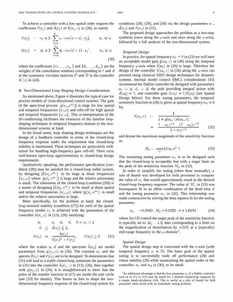
Spatial DesignThe spatial design step is concerned with the -axis (with
temporal frequency ! = 0). The basic goal of the spatialtuning is to successfully trade off performance (28) androbust stability (29) while maintaining the spatial order of thecontroller, nc and nd in (30), to be small.
3An additional advantage is that the free parameter c of a Dahlin controllersuch as in (7) or (13) may be tuned for a desired closed-loop response bya simple hand-calculation (34). This is useful as a rule of thumb for fieldpersonnel when faced with an immediate tuning problem.
IEEE TRANSACTIONS ON CONTROL SYSTEMS TECHNOLOGY 2003 9
νl νh
β=0.2
Spatial Frequency, ν
Mod
el G
ain,
|b(ν
)|
0.2
0.4
0.6
0.8
1.0
00
Fig. 5. Illustration of the definition of the low spatial frequency limit l wherejb(l)j =
p2=2 and the high spatial frequency limit h where jb(h)j =
for = 0:2 in terms of the steady-state model gain in (26). (This curve wastaken from the ! = 0 axis of the surface plot of the example in Figure 4.)
As mentioned in Subsection II-C, the smoothing operationhas only two degrees of freedom. We initially set the order ofthe Blackman window to be the smallest allowed with nd = 2.Setting the constant to be small = 0:01 then allows thecontroller pole d(j) in (26) to be computed as a function ofspatial frequency by (10), (30) with coefficients,
dl =
1 + (h1 1) l = 1 hl l = 2; : : : ; nd
(35)
where the scalars hl with l = 1; : : : ; nd are defined by alowpass Blackman window of order nd as described in (11).
For the majority of CD processes, a robust stability margin = 0:2
G(z) 1
has proven to be acceptable. Then, given
smoothing spectrum d(j) and Dahlin controller parametersc, ac, dc, it remains to design the controller gain c(j) withrespect to performance (28) and robust stability (29).
As with traditional loop shaping, these requirements do notconflict since they are applied at different spatial frequencies.At low spatial frequencies , the process gain b(j) is largerelative to the model uncertainty and the closed-loop per-formance is important, while at high spatial frequencies , theprocess gain b(j) is small relative to the model uncertainty and robustness is more important.
In characterizing the design, it is useful to define two spatialfrequency limits as illustrated in Figure 5. The low frequencylimit l was developed in practical cross-directional control tobe the frequency at which the model gain rolls off to
p2=2
of its maximum value4,
jb(l)j =p2
2; (36)
4Strictly speaking the spatial frequency array is defined only on the discretevalues f1; : : : ; ng, and interpolation is used to define the values l and hin (36) and (37). This interpolation is of little practical importance as thesefrequencies are used as target values.
and the minimum requirement in the papermaking industryis that a cross-directional controller will remove ‘all’ steady-state variability with a spatial frequency smaller than l in(36). This limit will be used constructively in the controllersynthesis algorithm below.
The high spatial frequency limit h is derived as the lowestfrequency for which the process model gain is smaller thanthe magnitude of the uncertainty in (18) or (29),
jb(h)j = (37)
The high frequency h defines the spatial frequency limitbeyond which we cannot guarantee any performance improve-ment with a feedback controller due to the uncertainty beinglarger than the model gain [5].
In [33] the detailed calculation of the array r( j) is com-puted in terms of the process gain spectrum b(j), but is notrepeated here. It is enough to understand that typically,
performance: r(j)! 0 for low j
robust stability: r(j) > 0 for high j (38)
Then the target controller gain is constructed such that
c(j) =b(j)
b(j)2 + r(j)(39)
In general, the controller gain designed frequency-by-frequency such as c(j) in (39) will not satisfy the require-ment of a low spatial order (30).
The synthesis step outlined in (38) and (39) is then followedby an order reduction operation where a low-order spectrumc(j) is fit to the target high-order spectrum c(j) in (39)(compare Theorem 4 in [32]). We expand the spectrum andcompute the first nc terms,
ci =1
n
nXj=1
c(j) cos[(i 1) j ]; i = 1; : : : ; nc (40)
where nc is the spatial order of C in (30). Equations (38)–(40)outline the “synthesis” routine referred to in Subsection V-Cbelow.
Finally, the spectrum corresponding to the reduced-orderdecoupling operator is created using,
c(j) = c1 + 2 ncXi=2
ci cos[(i 1) j ]; (41)
AnalysisThe above design has resulted in a distributed feedback
controller with low spatial order nc; nd n in (30). It remainsto verify that the robust stability condition (29) is satisfied forthe maximum over all spatial and temporal frequencies f; !g.The closed-loop performance of the system is presented interms of the performance frequencies 90 and !90 as describedin Subsection V-A above.
IEEE TRANSACTIONS ON CONTROL SYSTEMS TECHNOLOGY 2003 10
C. Controller Tuning Algorithm
This section contains an overview of the main componentsof the algorithms for two-dimensional loop shaping for cross-directional controller tuning.
Phase I: Initialization1) Given an identified model in (3) compute the model
parameters b(j), a and d in (26).2) Set controller parameters ac = a, dc = d in (7) and
initialize c with target sensitivity function peak Ms =1:2 in (34).
3) Initialize low and high limits l = 0:0005 and h =0:06. Initialize = (l+h)=2 and the Blackman filterorder nd = 2 in (35) and compute d(j) in (26), (30).
4) Initialize target stability margin = 0:2 and controllerspatial order nc = 10. (This spatial order has been foundto be large enough to cover practical cases.)
5) Call “synthesis” routine (38)–(40) to computefc1; : : : ; c10g.
6) Reduce the value of nc such that the sequence ofcoefficients fc1; : : : ; cncg changes sign at most once.
7) Using the model gain b(j) computed in Phase I, calcu-late the low and high spatial frequency limits l in (36)and h in (37).
8) Define the target frequency = (l + h)=2 andtolerance = (h l)=20.
Phase II: Tuning Iteration1) Set = (l+h)=2 in (35) and call “synthesis” routine
(38)–(40) to compute fc1; : : : ; cncg.2) Compute 90 on the -axis (! = 0) as the highest spatial
frequency for which the performance condition (28) issatisfied for p(; 0) = 10.
3) Is j90 j < ? If YES, then goto 6. If NO, thencontinue.
4) If 90 > , then set l = and goto 1.5) If 90 < , then set h = and goto 1.6) Extract the controller parameters fc1; : : : ; cncg,
fd1; : : : ; dndg, c, ac, dc.7) Verify the closed-loop stability of the associated trun-
cated Toeplitz system.8) Transfer the controller parameters to the working cross-
directional control system.
Phase III: (Optional) Direct Modification by the User1) Via the graphical interface, the user is permitted to
change: the spatial order of the controller decouplingnc, or actuator profile smoothing nd in (30), the targetstability margin in (29), and the values of in (35)and c in (13) and (26).
2) Call “synthesis” routine (38)–(40) to computefc1; : : : ; cncg.
3) Check that l < 90 < h.4) If NO, then a warning is presented to the user to return
to 1.5) Extract the controller parameters fc1; : : : ; cncg,
fd1; : : : ; dndg, ac, dc.
6) Verify the closed-loop stability of the associated trun-cated Toeplitz system.
7) Transfer the controller parameters to the working cross-directional control system.
VI. TWO INDUSTRIAL APPLICATIONS
A. System 1: A Closed-Loop Unstable Slice Lip System
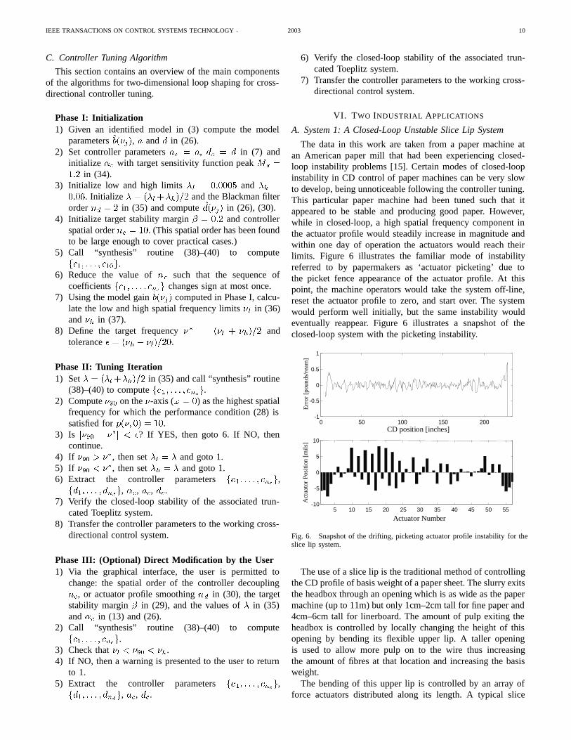
The data in this work are taken from a paper machine atan American paper mill that had been experiencing closed-loop instability problems [15]. Certain modes of closed-loopinstability in CD control of paper machines can be very slowto develop, being unnoticeable following the controller tuning.This particular paper machine had been tuned such that itappeared to be stable and producing good paper. However,while in closed-loop, a high spatial frequency component inthe actuator profile would steadily increase in magnitude andwithin one day of operation the actuators would reach theirlimits. Figure 6 illustrates the familiar mode of instabilityreferred to by papermakers as ‘actuator picketing’ due tothe picket fence appearance of the actuator profile. At thispoint, the machine operators would take the system off-line,reset the actuator profile to zero, and start over. The systemwould perform well initially, but the same instability wouldeventually reappear. Figure 6 illustrates a snapshot of theclosed-loop system with the picketing instability.
0 50 100 150 200-1
-0.5
0
0.5
1
5 10 15 20 25 30 35 40 45 50 55-10
-5
0
5
10
CD position [inches]
Actuator Number
Act
uato
r Po
sitio
n [m
ils]
Err
or [
poun
ds/r
eam
]
Fig. 6. Snapshot of the drifting, picketing actuator profile instability for theslice lip system.
The use of a slice lip is the traditional method of controllingthe CD profile of basis weight of a paper sheet. The slurry exitsthe headbox through an opening which is as wide as the papermachine (up to 11m) but only 1cm–2cm tall for fine paper and4cm–6cm tall for linerboard. The amount of pulp exiting theheadbox is controlled by locally changing the height of thisopening by bending its flexible upper lip. A taller openingis used to allow more pulp on to the wire thus increasingthe amount of fibres at that location and increasing the basisweight.
The bending of this upper lip is controlled by an array offorce actuators distributed along its length. A typical slice
IEEE TRANSACTIONS ON CONTROL SYSTEMS TECHNOLOGY 2003 11
20 40 60 80 100 120 140 160 180 200 220−0.5
0
0.5
CD POSITION, [inches]
RE
SP
ON
SE
, [po
unds
/rea
m]
5 10 15 20 25 30 35 40 45 50 55−2
−1
0
1
2
ACTUATOR NUMBER
INP
UT
, [m
ils]
Fig. 7. The open-loop steady-state spatial response of the directory gradepaper sheet to changes in the slice lip actuators.
lip installation has n = 50 of such actuators in the array,but there exist installations with n = 118 or more slice lipactuators. The actuator spacing is quite variable depending onthe installation and is anywhere from 7.0cm to 20cm. Modernslice lip actuator dynamics are very fast compared with thescan time. The process dynamics are thus dominated by thesensor filtering and the dead time due to the transport delayfrom the actuators to the scanning sensor.
The slice lip itself is quite expensive, and much care is takento prevent damaging it due to excessive flexing and bending.Depending on the lip material, each actuator has a range ofat most 0.17mm-0.75mm. The industrial controller containsmany safety interlocks and an actuator setpoint profile isprevented from violating the bending constraints specified forthe slice lip. However, an actuator setpoint profile as illustratedin Figure 6 is cause for concern as the increased bending willshorten the life of the lip.
10-4
10-3
10-2
0
0.02
0.04
0.06
0.08
0.1
|k| < 6.25|k| > 6.25
Ωh
Ωh
ω [cycles/second]
ν[c
ycle
s/in
ch]
violation of robuststability condition
Fig. 8. The open-loop stability margin condition (42) is violated at lowtemporal frequencies ! and high spatial frequencies for the original(decentralized) controller in Table II for the slice lip system.
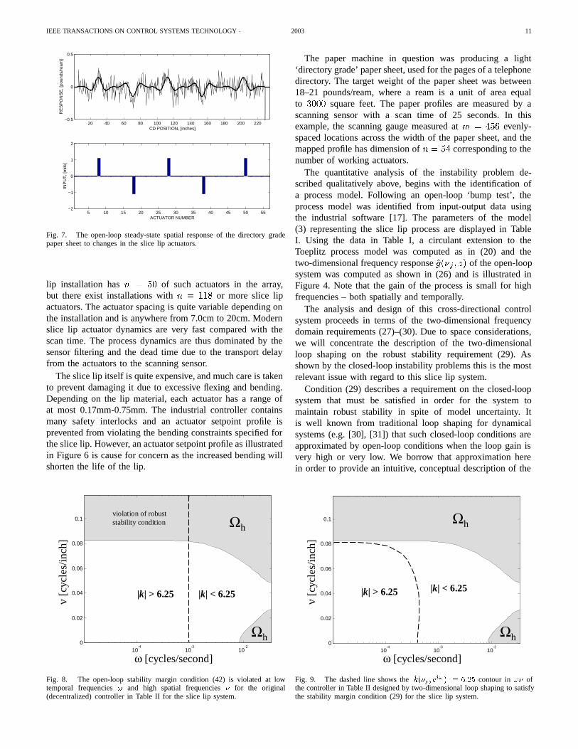
The paper machine in question was producing a light‘directory grade’ paper sheet, used for the pages of a telephonedirectory. The target weight of the paper sheet was between18–21 pounds/ream, where a ream is a unit of area equalto 3000 square feet. The paper profiles are measured by ascanning sensor with a scan time of 25 seconds. In thisexample, the scanning gauge measured at m = 456 evenly-spaced locations across the width of the paper sheet, and themapped profile has dimension of n = 54 corresponding to thenumber of working actuators.
The quantitative analysis of the instability problem de-scribed qualitatively above, begins with the identification ofa process model. Following an open-loop ‘bump test’, theprocess model was identified from input-output data usingthe industrial software [17]. The parameters of the model(3) representing the slice lip process are displayed in TableI. Using the data in Table I, a circulant extension to theToeplitz process model was computed as in (20) and thetwo-dimensional frequency response g(j ; z) of the open-loopsystem was computed as shown in (26) and is illustrated inFigure 4. Note that the gain of the process is small for highfrequencies – both spatially and temporally.
The analysis and design of this cross-directional controlsystem proceeds in terms of the two-dimensional frequencydomain requirements (27)–(30). Due to space considerations,we will concentrate the description of the two-dimensionalloop shaping on the robust stability requirement (29). Asshown by the closed-loop instability problems this is the mostrelevant issue with regard to this slice lip system.
Condition (29) describes a requirement on the closed-loopsystem that must be satisfied in order for the system tomaintain robust stability in spite of model uncertainty. Itis well known from traditional loop shaping for dynamicalsystems (e.g. [30], [31]) that such closed-loop conditions areapproximated by open-loop conditions when the loop gain isvery high or very low. We borrow that approximation herein order to provide an intuitive, conceptual description of the
10-4
10-3
10-2
0
0.02
0.04
0.06
0.08
0.1
|k| < 6.25|k| > 6.25
Ωh
Ωh
ω [cycles/second]
ν[c
ycle
s/in
ch]
Fig. 9. The dashed line shows the jk(j ; ei!)j = 6:25 contour in ! ofthe controller in Table II designed by two-dimensional loop shaping to satisfythe stability margin condition (29) for the slice lip system.
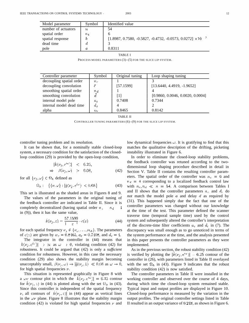
IEEE TRANSACTIONS ON CONTROL SYSTEMS TECHNOLOGY 2003 12
Model parameter Symbol Identified valuenumber of actuators n 54spatial order nb 6spatial response b [1.8987, 0.7580, -0.5827, -0.4732, -0.0573, 0.0272] 10 2dead time d 3pole a 0.8311
TABLE I
PROCESS MODEL PARAMETERS (3)–(5) FOR THE SLICE LIP SYSTEM.
Controller parameter Symbol Original tuning Loop shaping tuningdecoupling spatial order nc 1 3decoupling convolution c [57.1599] [13.6440, 4.4919, -1.9652]smoothing spatial order nd 1 4smoothing convolution d [1] [0.9860, 0.0046, 0.0020, 0.0004]internal model pole ac 0.7408 0.7344internal model dead time dc 4 2alpha c 0.8465 0.8142
TABLE II
CONTROLLER TUNING PARAMETERS (6)–(9) FOR THE SLICE LIP SYSTEM.
controller tuning problem and its resolution.It can be shown that, for a nominally stable closed-loop
system, a necessary condition for the satisfaction of the closed-loop condition (29) is provided by the open-loop condition,
jk(j ; ei!)j < 6:25;
) (j ; !) > 0:08; (42)
for all fj ; !g 2 h defined as
h :=f; !g : jg(j ; ei!)j < 0:08
(43)
This set is illustrated as the shaded areas in Figures 8 and 9.The values of the parameters in the original tuning of
the feedback controller are indicated in Table II. Since it iscompletely decentralized (having spatial order nc = nd = 1in (9)), then it has the same value,
k(j ; z) =57:1599
1 z1 c(z) (44)
for each spatial frequency j 2 f1; : : : ; 54g. The parametersof c(z) are given by c = 0:8465, ac = 0:7408, and dc = 4.
The integrator in the controller in (44) means thatjk(j ; ei!)j ! 1 as ! ! 0, violating condition (42) forrobustness. It could be argued that (42) is only a sufficientcondition for robustness. However, in this case the necessarycondition (29) also shows the stability margin becomingunacceptably small, (j ; !) ! jg(j ; 1)j 0:08 as ! ! 0,for high spatial frequencies .
This situation is represented graphically in Figure 8 witha ! contour plot in which the jk(j ; ei!)j = 6:25 contourfor k(j ; z) in (44) is plotted along with the set h in (43).Since this controller is independent of the spatial frequency, all contours of jk(j ; z)j in (44) appear as vertical linesin the ! plane. Figure 8 illustrates that the stability margincondition (42) is violated for high spatial frequencies and
low dynamical frequencies !. It is gratifying to find that thismatches the qualitative description of the drifting, picketinginstability illustrated in Figure 6.
In order to eliminate the closed-loop stability problems,the feedback controller was retuned according to the two-dimensional loop shaping procedure described in detail inSection V. Table II contains the resulting controller param-eters. The spatial order of the controller was nc = 6 andnd = 4 corresponding to a localized feedback control lawwith nc; nd n = 54. A comparison between Tables Iand II shows that the controller parameters ac and dc donot match the model pole a and delay d as required by(31). This happened simply due the fact that one of thecontroller parameters was changed without our knowledgeat the time of the test. This parameter defined the scannertraverse time (temporal sample time) used by the controlsystem and subsequently altered the controller’s interpretationof the discrete-time filter coefficients ac and dc in (7). Thediscrepancy was small enough as to go unnoticed in terms ofthe system performance at the time, and the analysis presentedin this paper presents the controller parameters as they wereimplemented.
As in the previous section, the robust stability condition (42)is verified by plotting the jk(j ; ei!)j = 6:25 contour of thecontroller in (26), with parameters listed in Table II overlayedwith the set h in (43). Figure 9 indicates that the robuststability condition (42) is now satisfied.
The controller parameters in Table II were installed in theworking controller and observed over the course of 4 days,during which time the closed-loop system remained stable.Typical input and output profiles are displayed in Figure 10.Closed-loop performance is measured by the variation in theoutput profiles. The original controller settings listed in TableII resulted in an output variance of 0:248, as shown in Figure 6.
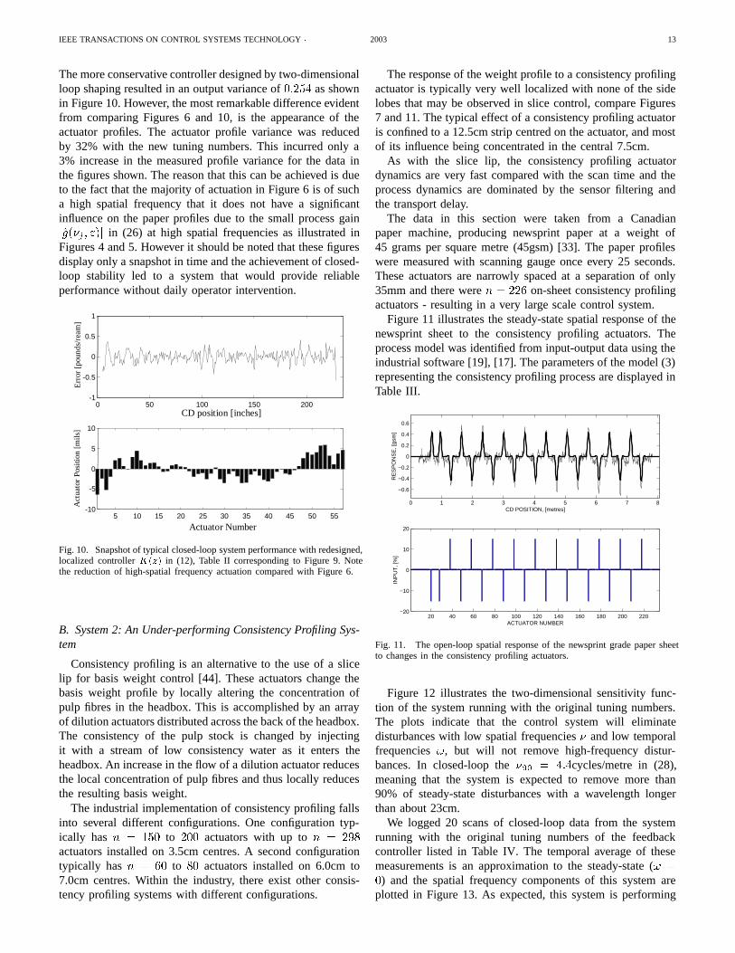
IEEE TRANSACTIONS ON CONTROL SYSTEMS TECHNOLOGY 2003 13
The more conservative controller designed by two-dimensionalloop shaping resulted in an output variance of 0:254 as shownin Figure 10. However, the most remarkable difference evidentfrom comparing Figures 6 and 10, is the appearance of theactuator profiles. The actuator profile variance was reducedby 32% with the new tuning numbers. This incurred only a3% increase in the measured profile variance for the data inthe figures shown. The reason that this can be achieved is dueto the fact that the majority of actuation in Figure 6 is of sucha high spatial frequency that it does not have a significantinfluence on the paper profiles due to the small process gainjg(j ; z)j in (26) at high spatial frequencies as illustrated inFigures 4 and 5. However it should be noted that these figuresdisplay only a snapshot in time and the achievement of closed-loop stability led to a system that would provide reliableperformance without daily operator intervention.
0 50 100 150 200-1
-0.5
0
0.5
1
5 10 15 20 25 30 35 40 45 50 55-10
-5
0
5
10
CD position [inches]
Actuator Number
Act
uato
r Po
sitio
n [m
ils]
Err
or [
poun
ds/r
eam
]
Fig. 10. Snapshot of typical closed-loop system performance with redesigned,localized controller K(z) in (12), Table II corresponding to Figure 9. Notethe reduction of high-spatial frequency actuation compared with Figure 6.
B. System 2: An Under-performing Consistency Profiling Sys-tem
Consistency profiling is an alternative to the use of a slicelip for basis weight control [44]. These actuators change thebasis weight profile by locally altering the concentration ofpulp fibres in the headbox. This is accomplished by an arrayof dilution actuators distributed across the back of the headbox.The consistency of the pulp stock is changed by injectingit with a stream of low consistency water as it enters theheadbox. An increase in the flow of a dilution actuator reducesthe local concentration of pulp fibres and thus locally reducesthe resulting basis weight.
The industrial implementation of consistency profiling fallsinto several different configurations. One configuration typ-ically has n = 150 to 200 actuators with up to n = 298actuators installed on 3.5cm centres. A second configurationtypically has n = 60 to 80 actuators installed on 6.0cm to7.0cm centres. Within the industry, there exist other consis-tency profiling systems with different configurations.
The response of the weight profile to a consistency profilingactuator is typically very well localized with none of the sidelobes that may be observed in slice control, compare Figures7 and 11. The typical effect of a consistency profiling actuatoris confined to a 12.5cm strip centred on the actuator, and mostof its influence being concentrated in the central 7.5cm.
As with the slice lip, the consistency profiling actuatordynamics are very fast compared with the scan time and theprocess dynamics are dominated by the sensor filtering andthe transport delay.
The data in this section were taken from a Canadianpaper machine, producing newsprint paper at a weight of45 grams per square metre (45gsm) [33]. The paper profileswere measured with scanning gauge once every 25 seconds.These actuators are narrowly spaced at a separation of only35mm and there were n = 226 on-sheet consistency profilingactuators - resulting in a very large scale control system.
Figure 11 illustrates the steady-state spatial response of thenewsprint sheet to the consistency profiling actuators. Theprocess model was identified from input-output data using theindustrial software [19], [17]. The parameters of the model (3)representing the consistency profiling process are displayed inTable III.
0 1 2 3 4 5 6 7 8
−0.6
−0.4
−0.2
0
0.2
0.4
0.6
CD POSITION, [metres]
RE
SP
ON
SE
, [gs
m]
20 40 60 80 100 120 140 160 180 200 220−20
−10
0
10
20
ACTUATOR NUMBER
INP
UT
, [%
]
Fig. 11. The open-loop spatial response of the newsprint grade paper sheetto changes in the consistency profiling actuators.
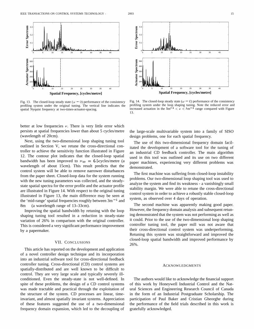
Figure 12 illustrates the two-dimensional sensitivity func-tion of the system running with the original tuning numbers.The plots indicate that the control system will eliminatedisturbances with low spatial frequencies and low temporalfrequencies !, but will not remove high-frequency distur-bances. In closed-loop the 90 = 4:4cycles/metre in (28),meaning that the system is expected to remove more than90% of steady-state disturbances with a wavelength longerthan about 23cm.
We logged 20 scans of closed-loop data from the systemrunning with the original tuning numbers of the feedbackcontroller listed in Table IV. The temporal average of thesemeasurements is an approximation to the steady-state (! =0) and the spatial frequency components of this system areplotted in Figure 13. As expected, this system is performing
IEEE TRANSACTIONS ON CONTROL SYSTEMS TECHNOLOGY 2003 14
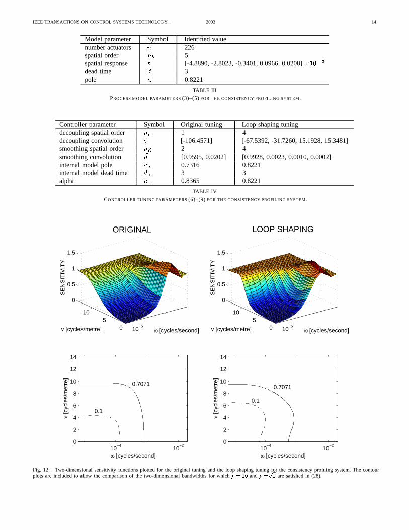
Model parameter Symbol Identified valuenumber actuators n 226spatial order nb 5spatial response b [-4.8890, -2.8023, -0.3401, 0.0966, 0.0208] 10 3dead time d 3pole a 0.8221
TABLE III
PROCESS MODEL PARAMETERS (3)–(5) FOR THE CONSISTENCY PROFILING SYSTEM.
Controller parameter Symbol Original tuning Loop shaping tuningdecoupling spatial order nc 1 4decoupling convolution c [-106.4571] [-67.5392, -31.7260, 15.1928, 15.3481]smoothing spatial order nd 2 4smoothing convolution d [0.9595, 0.0202] [0.9928, 0.0023, 0.0010, 0.0002]internal model pole ac 0.7316 0.8221internal model dead time dc 3 3alpha c 0.8365 0.8221
TABLE IV
CONTROLLER TUNING PARAMETERS (6)–(9) FOR THE CONSISTENCY PROFILING SYSTEM.
10−50
510
0
0.5
1
1.5
ω [cycles/second]
ORIGINAL
ν [cycles/metre]
SE
NS
ITIV
ITY
10−4
10−2
0
2
4
6
8
10
12
14
ω [cycles/second]
ν [c
ycle
s/m
etre
]
10−50
510
0
0.5
1
1.5
ω [cycles/second]
LOOP SHAPING
ν [cycles/metre]
SE
NS
ITIV
ITY
10−4
10−2
0
2
4
6
8
10
12
14
ω [cycles/second]
ν [c
ycle
s/m
etre
]
0.7071 0.7071
0.1
0.1
Fig. 12. Two-dimensional sensitivity functions plotted for the original tuning and the loop shaping tuning for the consistency profiling system. The contourplots are included to allow the comparison of the two-dimensional bandwidths for which p = 10 and p =
p2 are satisfied in (28).
IEEE TRANSACTIONS ON CONTROL SYSTEMS TECHNOLOGY 2003 15
0 5 10 15 20 25 30 35 400
0.1
0.2
0.3
0 5 10 15 20 25 30 35 400
100
200
300
400
500
Err
or S
pect
rum
Act
uato
r Sp
ectr
um
Spatial Frequency, [cycles/metre]
Fig. 13. The closed-loop steady state (! = 0) performance of the consistencyprofiling system under the original tuning. The vertical line indicates thespatial Nyquist frequency at two-times-actuator-spacing.
better at low frequencies . There is very little error whichpersists at spatial frequencies lower than about 5 cycles/metre(wavelength of 20cm).
Next, using the two-dimensional loop shaping tuning tooloutlined in Section V, we retune the cross-directional con-troller to achieve the sensitivity function illustrated in Figure12. The contour plot indicates that the closed-loop spatialbandwidth has been improved to 90 = 6:5cycles/metre (awavelength of about 15cm). This result predicts that thecontrol system will be able to remove narrower disturbancesfrom the paper sheet. Closed-loop data for the system runningwith the new tuning parameters was collected, and the steady-state spatial spectra for the error profile and the actuator profileare illustrated in Figure 14. With respect to the original tuningillustrated in Figure 13, the main difference may be seen atthe ‘mid-range’ spatial frequencies roughly between 3m1 and8m1 (a wavelength range of 13–33cm).
Improving the spatial bandwidth by retuning with the loopshaping tuning tool resulted in a reduction in steady-statevariation of 26% in comparison with the original controller.This is considered a very significant performance improvementby a papermaker.
VII. CONCLUSIONS
This article has reported on the development and applicationof a novel controller design technique and its incorporationinto an industrial software tool for cross-directional feedbackcontroller tuning. Cross-directional (CD) control systems arespatially-distributed and are well known to be difficult tocontrol. They are very large scale and typically severely ill-conditioned. Even the steady-state is not well-defined. Inspite of these problems, the design of a CD control systemswas made tractable and practical through the exploitation ofthe structure of the system. CD processes are linear, time-invariant, and almost spatially invariant systems. Appreciationof these features suggested the use of a two-dimensionalfrequency domain expansion, which led to the decoupling of
0 5 10 15 20 25 30 35 400
0.1
0.2
0.3
0 5 10 15 20 25 30 35 400
100
200
300
400
500
Err
or S
pect
rum
Act
uato
r Sp
ectr
um
Spatial Frequency, [cycles/metre]
Fig. 14. The closed-loop steady state (! = 0) performance of the consistencyprofiling system under the loop shaping tuning. Note the reduced error andincreased actuation in the 3m1 < < 8m1 range compared with Figure13.
the large-scale multivariable system into a family of SISOdesign problems, one for each spatial frequency.
The use of this two-dimensional frequency domain facil-itated the development of a software tool for the tuning ofan industrial CD feedback controller. The main algorithmused in this tool was outlined and its use on two differentpaper machines, experiencing very different problems wasdemonstrated.
The first machine was suffering from closed-loop instabilityproblems. Our two-dimensional loop shaping tool was used toanalyze the system and find its weakness - a vanishingly smallstability margin. We were able to retune the cross-directionalcontrol system in order to achieve a robustly stable closed-loopsystem, as observed over 4 days of operation.
The second machine was apparently making good paper.However, the frequency domain analysis and subsequent retun-ing demonstrated that the system was not performing as well asit could. Prior to the use of the two-dimensional loop shapingcontroller tuning tool, the paper mill was not aware thattheir cross-directional control system was underperforming.Retuning this system was straightforward and improved theclosed-loop spatial bandwidth and improved performance by26%.
ACKNOWLEDGMENTS
The authors would like to acknowledge the financial supportof this work by Honeywell Industrial Control and the Nat-ural Sciences and Engineering Research Council of Canadain the form of an Industrial Postgraduate Scholarship. Theparticipation of Paul Baker and Cristian Gheorghe duringthe performance of the field trials described in this work isgratefully acknowledged.
IEEE TRANSACTIONS ON CONTROL SYSTEMS TECHNOLOGY 2003 16
REFERENCES
[1] A.P. Featherstone and R.D. Braatz, “Input design for large-scale sheetand film processes,” Ind. Eng. Chem. Res., vol. 37, pp. 449–454, 1998.
[2] D.L. Laughlin, M. Morari, and R.D. Braatz, “Robust performance ofcross-directional control systems for web processes,” Automatica, vol.29, no. 6, pp. 1395–1410, 1993.
[3] S.R. Duncan, “The design of robust cross-directional control systemsfor paper making,” in Proc. of American Control Conf., Seattle, WA,USA, June 1995, pp. 1800–1805.
[4] S.R. Duncan, The Cross-Directional Control of Web Forming Processes,Ph.D. thesis, University of London, UK, 1989.
[5] A.P. Featherstone, J.G. VanAntwerp, and R.D. Braatz, Identification andControl of Sheet and Film Processes, Springer, 2000.
[6] K. Kristinsson and G.A. Dumont, “Cross-directional control on papermachines using gram polynomials,” Automatica, vol. 32, no. 4, pp.533–548, 1996.
[7] A. Rigopoulos, Application of Principal Component Analysis in theIdentification and Control of Sheet-Forming Processes, Ph.D. thesis,Georgia Institute of Technology, USA, 1999.
[8] W.P. Heath, “Orthogonal functions for cross-directional control of webforming processes,” Automatica, vol. 32, no. 2, pp. 183–198, 1996.
[9] S.-C. Chen and R.G. Wilhelm Jr., “Optimal control of cross-machinedirection web profile with constraints on the control effort,” in Proc. ofAmerican Control Conf., Seattle, June 1986.
[10] W.P. Heath and P.E. Wellstead, “Self-tuning prediction and control fortwo-dimensional processes. part 1: Fixed parameter algorithms,” Int. J.Control, vol. 62, no. 1, pp. 65–107, 1995.
[11] J. Fan, G.E. Stewart, and G.A. Dumont, “Model predictive cross-directional control using a reduced model,” in Control Systems 2002,Stockholm, Sweden, June 2002, pp. 65–69.
[12] J.U. Backstrom, C. Gheorghe, G.E. Stewart, and R.N. Vyse, “Con-strained model predictive control for cross directional multi-array pro-cesses,” Pulp and Paper Canada, vol. 102, no. 5, pp. T128–T131, May2001.
[13] J. Shakespeare, J. Pajunen, V. Nieminen, and T. Metsala, “Robustoptimal control of profiles using multiple CD actuator systems,” inControl Systems 2000, Victoria, BC, May 2000, pp. 306–310.
[14] G.E. Stewart, D.M. Gorinevsky, and G.A. Dumont, “Design of apractical robust controller for a sampled distributed parameter system,”in Proc. of IEEE Conference on Decision and Control, Tampa, FL, USA,December 1998, pp. 3156–3161.
[15] G.E. Stewart, P. Baker, D.M. Gorinevsky, and G.A. Dumont, “Anexperimental demonstration of recent results for spatially distributedcontrol systems,” in Proc. of American Control Conf., Arlington, VA,USA, June 2001, pp. 2216–2221.
[16] E.M. Heaven, I.M. Jonsson, T.M. Kean, M.A. Manness, and R.N. Vyse,“Recent advances in cross-machine profile control,” IEEE ControlSystems Magazine, pp. 36–46, October 1994.
[17] D.M. Gorinevsky, E.M. Heaven, C. Sung, and M. Kean, “Integratedtool for intelligent identification of CD process alignment shrinkage anddynamics,” Pulp and Paper Canada, vol. 99, no. 2, pp. 40–44, 1998.
[18] D.M. Gorinevsky, R.N. Vyse, and E.M. Heaven, “Performance analysisof cross-directional process control using multivariable and spectralmodels,” IEEE Trans. on Control Systems Technology, vol. 8, no. 4,pp. 589–600, July 2000.
[19] D.M. Gorinevsky and M. Heaven, “Performance-optimized appliedidentification of separable distributed-parameter processes,” IEEE Trans.Automat. Contr., vol. 46, no. 10, pp. 1584–1589, October 2001.
[20] D.M. Gorinevsky and C. Gheorghe, “Identification tool for cross-directional processes,” to appear in IEEE Trans. on Control SystemsTechnology, 2003.
[21] P.J. Davis, Circulant Matrices, Wiley, New York, 1979.[22] R.M. Gray, “Toeplitz and circulant matrices: A review,” http://ee-
www.stanford.edu/~gray/toeplitz.html, 2001.[23] K. Cutshall, “Cross-direction control,” in Paper Machine Operations,
Pulp and Paper Manufacture, 3rd ed., vol. 7, Atlanta and Montreal,Chap. XVIII 1991, pp. 472–506.
[24] D.W. Kawka, A Calendering Model for Cross-Direction Control, Ph.D.thesis, McGill University, Montreal, Canada, 1998.
[25] S.R. Duncan, P.E. Wellstead, and M.B. Zarrop, “Actuation, sensing,and two-dimensional control algorithms: Fundamental limitations onachievable bandwidths in MD/CD control,” in Tappi Proc. ProcessControl, Electrical and Information Conf., Vancouver, BC, Canada,March 1998, pp. 245–258.
[26] J.C. Skelton, P.E. Wellstead, and S.R. Duncan, “Distortion of webprofiles by scanned measurements,” in Control Systems 2000, Victoria,BC, May 2000, pp. 311–314.
[27] S.-C. Chen, “Full-width sheet property estimation from scanning mea-surements,” in Control Systems ’92, Whistler, BC, Canada, September1992, pp. 123–130.
[28] S.R. Duncan and P. Wellstead, “Processing data from scanning gaugeson industrial web processes,” submitted to Automatica, August 2002.
[29] G.E. Stewart, J.U. Backstrom, P. Baker, C. Gheorghe, and R.N. Vyse,“Controllability in cross-directional processes: Practical rules for anal-ysis and design,” Pulp and Paper Canada, vol. 103, no. 8, pp. 32–38,August 2002.
[30] S. Skogestad and I. Postlethwaite, Multivariable Feedback Control:Analysis and Design, Wiley, New York, 1996.
[31] K. Zhou, J.C. Doyle, and K. Glover, Robust and Optimal Control,Prentice Hall, New Jersey, 1996.
[32] G.E. Stewart, D.M. Gorinevsky, and G.A. Dumont, “Two-dimensionalloop shaping,” to appear in Automatica, vol. 39, no. 5, May 2003.
[33] G.E. Stewart, Two Dimensional Loop Shaping: Controller Design forPaper Machine Cross-Directional Processes, Ph.D. thesis, Departmentof Electrical and Computer Engineering, University of British Columbia,Vancouver, Canada, 2000.
[34] B. Bamieh, F. Paganini, and M. Dahleh, “Distributed control of spatiallyinvariant systems,” IEEE Trans. Automat. Contr., vol. 47, no. 7, pp.1091–1107, July 2002.
[35] G. Ayres and F. Paganini, “Convex synthesis of localized controllers forspatially invariant systems,” Automatica, vol. 38, no. 3, March 2002.
[36] R. D’Andrea and G.E. Dullerud, “Distributed control of spatiallyinterconnected systems,” IEEE Trans. Automat. Contr., submitted.
[37] D.M. Gorinevsky and G. Stein, “Structured uncertainty analysis ofrobust stability for spatially distributed systems,” in Proc. of IEEEConference on Decision and Control, Sydney, Australia, December2000.
[38] S.-C. Chen, P. Tran, and K. Kristinsson, “Closed-loop analysis andtuning of cross-direction (CD) control for sheet-forming processes,” inProc. of IFAC Adchem, Banff, Canada, June 1997, pp. 389–395.
[39] S.R. Duncan and G.F. Bryant, “The spatial bandwidth of cross-directional control systems for web processes,” Automatica, vol. 33,no. 2, pp. 139–153, 1997.
[40] C. Langbort and R. D’Andrea, “Imposing boundary conditions for aclass of spatially-interconnected systems,” in submitted to AmericanControl Conf., Denver, Colorado, USA, June 2003.
[41] S. Mijanovic, G.E. Stewart, G.A. Dumont, and M.S. Davies, “Stability-preserving modification of paper machine cross-directional control nearspatial domain boundaries,” in IEEE Conf. Decision and Control, LasVegas, Nevada, USA, December 2002.
[42] M. Hovd and S. Skogestad, “Control of symmetrically interconnectedplants,” Automatica, vol. 30, no. 6, pp. 957–973, 1994.
[43] G.A. Dumont, “Analysis of the design and sensitivity of the Dahlinregulator,” Technical report, Pulp and Paper Research Institute ofCanada, PPR 345 1981.
[44] R. Vyse, C. Hagart-Alexander, E.M. Heaven, J. Ghofraniha, andT. Steele, “New trends in CD weight control for multi-ply applications,”in TAPPI Update on Multiply Forming Forum, Atlanta, Georgia, USA,February 1998.
IEEE TRANSACTIONS ON CONTROL SYSTEMS TECHNOLOGY 2003 17
PLACEPHOTOHERE
Gregory E. Stewart (S’97, M’00) received theB.Sc. degree in Physics in 1994 and the M.Sc. degreein Applied Mathematics in 1996 from DalhousieUniversity in Halifax, and the PhD degree from theDepartment of Electrical and Computer Engineeringat the University of British Columbia in Vancouverin 2000.
He currently holds the position of Senior ControlEngineer for Honeywell Industry Solutions and hasheld an Adjunct Professor appointment in the De-partment of Electrical and Computer Engineering at
the University of British Columbia since 2000. His research interests are inthe development and use of theory for practical implementation of advancedcontrol strategies. His designs currently reside on more than 60 industrialinstallations.
Dr Stewart has received the IEEE “Control Systems Technology Award”(with Dimitry Gorinevsky), an NSERC “University-Industry Synergy Awardfor Innovation” (with Guy Dumont), and two Honeywell “Technical Achieve-ment” awards (with Cristian Gheorghe).
PLACEPHOTOHERE
Dimitry M. Gorinevsky is a Senior Staff Scientistwith Honeywell Labs (Aerospace Electronics Sys-tems) and a Consulting Professor of Electrical Engi-neering with Information Systems Laboratory, Stan-ford University. He received Ph.D. from MoscowLomonosov University and M.S. from the MoscowInstitute of Physics and Technology. He was withthe Russian Academy of Sciences in Moscow, anAlexander von Humboldt Fellow in Munich, andwith the University of Toronto. Before joining Hon-eywell Labs he worked on paper machine control
with Honeywell-Measurex and was an Adjunct Professor of Electrical andComputer Engineering at the University of British Columbia, Vancouver,Canada. His interests are in advanced information and control systemsapplications across many industries. He has authored a book, more than 110reviewed technical papers and several patents. He is an Associate Editorof IEEE Transactions on Control Systems Technology. Together with GregStewart, he is a recipient of 2002 Control Systems Technology award of theIEEE Control Systems Society, in part, for industrial applications of the workdescribed in this paper.
PLACEPHOTOHERE
Guy A. Dumont received his Diplome d’Ingenieurfrom ENSAM, Paris, France in 1973 and hisPh.D., Electrical Engineering from McGill Univer-sity, Montreal in 1977. In 1973-74, and then againfrom 1977 to 1979, he worked for Tioxide France.From 1979 to 1989, he was with Paprican, firstin Montreal and then in Vancouver. In 1989, hejoined the Department of Electrical and ComputerEngineering at the University of British Columbiawhere he is a Professor and leads the Process ControlGroup. From 1989 to 1999, he held the Papri-
can/NSERC Chair in Process Control. In 2000-2002, he was also AssociateDean, Research for the Faculty of Applied Science. Guy Dumont was awardeda 1979 IEEE Transactions on Automatic Control Honourable Paper Award;a 1985 Paprican Presidential Citation; a 1990 UBC Killam research Prize;the 1995 CPPA Weldon Medal; the 1998 Universal Dynamics Prize forLeadership in Process Control Technology; the IEEE Control Systems Society1998 Control Systems Technology Award; and NSERC Synergy Awards inboth 1999 and 2002. He is a Fellow of the IEEE and the BC AdvancedSystems Institute, and a member of ISA, PAPTAC and TAPPI. His currentresearch interests are: adaptive control, distributed parameter system control,control loop performance monitoring, predictive control, with applications tothe process industries, mainly pulp and paper, and more recently to biomedicalengineering.