Identifying Extreme Observations, Outliers and Noise in ... · of Computation Science and Artificial Intelligence, University of the Basque Country UPV/EHU, Donostia, Spain; 3Department

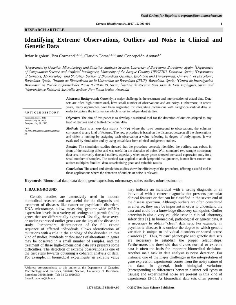
Send Orders for Reprints to [email protected]

Current Bioinformatics, 2017, 12, 000-000 1

RESEARCH ARTICLE

1574-8936/17 $58.00+.00 © 2017 Bentham Science Publishers

Identifying Extreme Observations, Outliers and Noise in Clinical and Genetic Data

Itziar Irigoien2, Bru Cormand3,4,5,6, Claudio Toma3,4,5,7 and Concepción Arenas1,*

1Department of Genetics, Microbiology and Statistics, Statistics Section, University of Barcelona, Barcelona, Spain; 2Department

of Computation Science and Artificial Intelligence, University of the Basque Country UPV/EHU, Donostia, Spain; 3Department

of Genetics, Microbiology and Statistics, Section of Biomedical Genetics, Evolution and Development, University of Barcelona,

Barcelona, Spain; 4Institut de Biomedicina de la Universitat de Barcelona (IBUB), Barcelona, Spain; 5Centro de Investigación

Biomèdica en Red de Enfermedades Raras (CIBERER), Spain; 6Institut de Recerca Sant Joan de Déu, Esplugues, Spain and 7Neuroscience Research Australia, Sydney, New South Wales, Australia

Abstract: Background: Currently, a major challenge is the treatment and interpretation of actual data. Data

sets are often high-dimensional, have small number of observations and are noisy. Furthermore, in recent

years, many approaches have been suggested for integrating continuous with categorical/ordinal data, in

order to capture the information which is lost in independent studies.

Objective: The aim of this paper is to develop a statistical tool for the detection of outliers adapted to any

kind of features and to high-dimensional data.

Method: Data is an nxp data matrix (n<<p) where the rows correspond to observations, the columns

correspond to any kind of features. The new procedure is based on the distances between all the observations

and offers a ranking by assigning each observation a value reflecting its degree of outlyingness. It was

evaluated by simulation and by using actual data from clinical and genetic studies.

Results: The simulation studies showed that the procedure correctly identified the outliers, was robust in

front of the masking effect and was useful in the detection of noise. With simulated two-sample microarray

data sets, it correctly detected outliers, especially when many genes showed increased expression only for a

small number of samples. The method was applied to adult lymphoid malignancies, human liver cancer and

autism multiplex families’ data sets obtaining good and valuable results.

Conclusion: The actual and simulation studies show the efficiency of the procedure, offering a useful tool in

those applications where the detection of outliers or noise is relevant.

A R T I C L E H I S T O R Y

Received: June 4, 2015

Revised: July 24, 2015

Accepted: July 26, 2015

DOI:

10.2174/15748936116661606061610

31

Keywords: Biomedical data, data depth, gene expression, microarray, noise, outlier, robust estimation.

1. BACKGROUND

Genetic studies are extensively used in modern biomedical research and are useful for the diagnosis and treatment of diseases like cancer or psychiatric disorders. DNA microarrays allow measuring genome-wide mRNA expression levels in a variety of settings and permit finding genes that are differentially expressed. Usually, these over- or under-expressed outlier genes are the key of the disease in study. Furthermore, determination of the full exome sequence of affected individuals allows identification of mutations with a role in the etiology of the disorder. In this kind of studies, hundreds or thousands of alterations in genes may be observed in a small number of samples, and the treatment of these high-dimensional data sets presents some difficulties. The detection of extreme observations is one of the first steps towards obtaining a coherent analysis of data. For example, in biomedical experiments an extreme value

*Address correspondence to this author at the Department of Genetics,

Microbiology and Statistics, Statistic Section, University of Barcelona, Barcelona 08028 Spain; Tel: 34 93 4020950;

E-mail: [email protected]

may indicate an individual with a wrong diagnosis or an individual with a correct diagnosis that presents particular clinical features or that can be classified in the severe end of the disease spectrum. Although outliers are often considered as an error, they may be important in order to understand the data and could be a knowledge discovery standpoint. Outlier detection is also a very valuable issue in clinical laboratory safety data [1]. In biomedical, pathological or genetic data, it is necessary to obtain “clean” data sets. For example, in psychiatric disease, it is unclear the degree to which genetic variation is unique to individual disorders or shared across disorders [2]. Thus, “clean” phenotypic and genetic data sets are necessary to establish the proper relationships. Furthermore, the threshold that divides normal or extreme data is often the basis for important biomedical decisions. Another main task in data analysis is noise detection. For instance, one of the major challenges in the interpretation of gene expression experiments comes from the noisy nature of the data. In general, both biological variations (corresponding to differences between distinct cell types or tissues) and experimental noise are present in this kind of experiments [3-5]. As biomedical data sets often present a

2 Current Bioinformatics, 2017, Vol. 12, No. 2 Irigoien et al.

large amount of noise, detecting and removing noisy instances can greatly improve the analysis. However, it is difficult to remove noise because we do not know exactly what the noise is. In a data set, noise can be defined as a datum apparently inconsistent with the rest of the data. Thus, its detection can be treated as an outlier detection problem.

The usual scenario with actual data is working without any information about the distribution of the data and only the experience of the biomedical research can determine if a value is an outlier (it has a low probability that it originates from the same statistical distribution as the other observations in the data set) or an extreme observation (might have a low probability of occurrence, but cannot be statistically shown to originate from a different distribution than the rest of the data). Furthermore, data sets for genetic studies or medical imaging usually contain more dimensions than observations, and in diagnosis or classification of diseases there are several types of information (for example genomic and clinical). For all these reasons, methods for outlying detection for high-dimensional data with observations measured on different kind of attributes and with unknown data distribution are desirable.

Many methods have been proposed for outlier detection when only one feature is measured (univariate case), but they are not useful for multivariate data. For the multivariate case, it is important to take into account the relationships between all the features in order to identify an observation as outlier. For example, in medical data, a patient whose clinical measurements do not follow the same pattern of relationship of the other patients may be detected as an outlier using a multivariate method. However, it may not be identified as an outlier when features are considered one at a time. There is much literature on outliers' detection, and extensive reviews can be found [6-10]. It is known that outlier detection algorithms for multivariate data depend on several factors: whether or not the data set is multivariate normal; the dimension of the data set; the data structure dimension and size; the time constrain with regard to single versus sequential identifiers (single-step procedures identify all outliers at once as opposed to successive elimination or addition of datum. In sequential procedures, at each step, one observation is analyzed for being an outlier); the type of the outliers; the proportion of outliers in the data set and the outlier's degree of contamination (outlyingness). For this reason, a direct comparison between them is not possible [1, 11]. The parametric multivariate methods assume a known underlying distribution or are based on the estimation of some parameters ([12-15]). However, these methods are often unsuitable for high-dimensional data sets (with the number of dimensions larger than the number of observations, as the covariance matrix becomes singular) which are usually present in medical imaging or genetic data (the number of genes is much larger than the number of samples). Recently, a parametric approach that utilizes inherent properties of principal component decomposition suitable for large data sets was developed [16]. The non-parametric methods are model-free and are especially attractive in microarray data which is often noisy and not normally distributed [17]. The distance-based procedures which are based on local distances [18] are, perhaps, the most popular among the non-parametric methods. However, depending on the definition of the distance-based outlier

function, these methods present some difficulties [19, 20]: the determination of certain parameters; the lack of a ranking for the outliers; the fact that they only consider the distance to some neighbors ignoring information about closer observations or the fact that its calculation is time consuming. Other non-parametric methods are based on depth functions, which can generate contours following the shape of the data sets [21, 22]. A depth of an observation is a nonnegative number, which measures the centrality of the observation. That is, depth in the sample version reflects the position of the observation with respect to the data cloud. There are many possibilities to define a data depth function ([23-26]), but the computation of the most popular depth functions is very slow, in particular for high dimensional data where the time needed for execution grows rapidly. In [27], a new less-computer intensive depth function based on distances was presented but the authors did no study its use in the outlier identification context. Recently, other authors have proposed methods to detect cancer genes with a subject of over- or under-expressed outlier disease samples ([28- 32]). These methods are specially designed to detect genes that show increased expression only for a small number of disease samples and all of them require continuous data.

In this paper, we propose a statistical tool for the detection of outliers adapted to any kind of features and high-dimensional data. The procedure, which does not require a known underlying distribution or parameter estimations, offers a ranking by assigning each observation a value reflecting its degree of outlyingness, and needs small computation time.

2. METHODS

The starting point is an 𝑛𝑥𝑝 data matrix where the rows correspond to observations (individuals, samples) and the columns correspond to any kind of features to be measured which can be continuous, binary or multiattribute data (genes, clinical/pathological features) and 𝑝 can be much larger than the size of the sample 𝑛 (𝑛 ≪ 𝑝). Recently, in [27] was proposed a depth function I for this kind of multivariate data, providing a way of measuring how representative or central an observation is within a sample. The notion of depth assigns for every observation a real number satisfying that the closer a point is to the mass center the higher its depth is. Thus, large depth values are related with deeper observations, and observations can be ordered from center outward. The definition of this depth function I is based in concepts that we briefly present.

Let G be a group that is represented by a 𝑝 -random vector 𝐘 = (𝑌1, … , 𝑌𝑝), with values in a metric space 𝑆 ⊂ 𝑅𝑝 and a probability density 𝑓 with respect to a suitable measure 𝜆. Let 𝛿 be a distance function between any pair of observations, 𝛿𝑖𝑗 = 𝛿(𝒚𝑖 , 𝒚𝑗). The geometric variability of G with respect to 𝛿 is a general measure of dispersion of G and is defined in [33] by,

𝑉(𝐺) =1

2∫ 𝛿2(𝒚𝑖 , 𝒚𝑗)𝑓(𝒚𝑖)𝑓(𝒚𝑗)

𝑆𝑥𝑆

𝜆(𝑑𝒚𝑖)𝜆(𝑑𝒚𝑗).

When 𝛿 is the Euclidean distance, 𝑉(𝐺) = 𝑡𝑟(Σ) with Σ=cov(Y). The geometric variability is as a variant of Rao's diversity coefficient [34].

Identifying Extreme Observations, Outliers and Noise in Clinical and Genetic Data Current Bioinformatics, 2017, Vol. 12, No. 2 3

The proximity function of an observation 𝒚 to G is

defined in [33] by,

Φ2(𝒚, 𝐺) = ∫ 𝛿2(𝑆

𝒚, 𝒚𝒋)𝑓(𝒚𝒋)𝜆(𝑑𝒚𝒋) − 𝑉(𝐺).

As in applied problems the probability distribution for Y is usually unknown, estimators are needed. Given a sample of size n, 𝒚1, … , 𝒚𝑛 , natural estimators for the geometric variability and the proximity function are, respectively,

�̂�(𝐺) =1

2𝑛2∑ 𝛿2(𝒚𝑖 , 𝒚𝑗),

𝑖,𝑗

and

Φ̂2(𝒚, 𝐺) =1

𝑛∑ 𝛿2(𝒚, 𝒚𝒋) −

𝑖�̂�(𝐺).

See [35] for a review of these concepts and for applications see [36], [37] and references therein.

In [27] a depth function based on these concepts was defined. For each observation 𝒚𝑖 the depth function 𝐼(𝒚𝑖, 𝐺) is given by,

𝐼(𝒚𝑖 , 𝐺) = [1 +Φ2(𝒚𝑖,𝐺)

𝑉(𝐺)]

−1

. (1)

Function I takes values in [0,1] and according to [25], function I is a type C depth function. Furthermore, it verifies the following desirable properties. Maximality at center: for a distribution having a uniquely defined “center” (e.g., the observation of symmetry with respect to some notion of symmetry), the depth function should attain maximum value at this center. Monotonicity relative to the deepest observation: as an observation moves away from the deepest observation (the observation at which the depth function attains maximum value; in particular, for a symmetric distribution, the center) along any fixed ray through the center, the depth at the observation should decrease monotonically. Vanishing at infinity: the depth of an observation 𝒚 should approach zero as ‖𝒚‖ approaches infinity. Moreover, depending on the data and the selected

distance, it is affine invariant (the depth of an observation should not depend on the underlying coordinate system or, in particular, on the scales of the underlying measurements).

As I is a depth function, it assigns to any observation a degree of centrality, thus a small value of I, or equivalently a large value of 𝑂 = 1/𝐼, suggests a possible outlier observation. Note that by (1),

𝑂(𝒚𝑖 , 𝐺) =1

𝑛∑ 𝛿2(𝒚𝒊,𝒚𝒋)𝑗

1

2𝑛2 ∑ 𝛿2(𝒚𝑗,𝒚𝑘)𝑗,𝑘 (2)

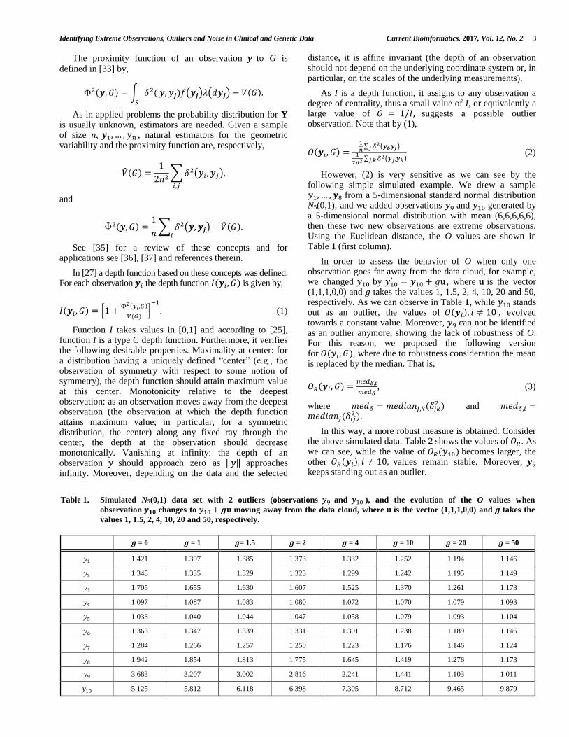
However, (2) is very sensitive as we can see by the following simple simulated example. We drew a sample 𝒚1, … , 𝒚8 from a 5-dimensional standard normal distribution N5(0,1), and we added observations 𝒚9 and 𝒚10 generated by a 5-dimensional normal distribution with mean (6,6,6,6,6), then these two new observations are extreme observations. Using the Euclidean distance, the O values are shown in Table 1 (first column).

In order to assess the behavior of O when only one observation goes far away from the data cloud, for example, we changed 𝒚10 by 𝒚10

′ = 𝒚10 + 𝑔𝐮, where 𝐮 is the vector (1,1,1,0,0) and 𝑔 takes the values 1, 1.5, 2, 4, 10, 20 and 50, respectively. As we can observe in Table 1, while 𝒚10 stands out as an outlier, the values of 𝑂(𝒚𝑖), 𝑖 ≠ 10 , evolved towards a constant value. Moreover, 𝒚9 can not be identified as an outlier anymore, showing the lack of robustness of O. For this reason, we proposed the following version for 𝑂(𝒚𝑖 , 𝐺), where due to robustness consideration the mean is replaced by the median. That is,

𝑂𝑅(𝒚𝑖 , 𝐺) =𝑚𝑒𝑑𝛿,𝑖

𝑚𝑒𝑑𝛿, (3)

where 𝑚𝑒𝑑𝛿 = 𝑚𝑒𝑑𝑖𝑎𝑛𝑗,𝑘(𝛿𝑗𝑘2 ) and 𝑚𝑒𝑑𝛿,𝑖 =

𝑚𝑒𝑑𝑖𝑎𝑛𝑗(𝛿𝑖𝑗2 ).

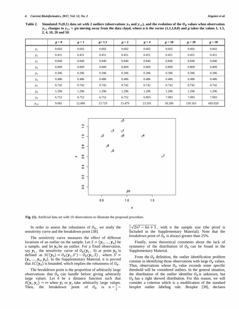
In this way, a more robust measure is obtained. Consider the above simulated data. Table 2 shows the values of 𝑂𝑅 . As we can see, while the value of 𝑂𝑅(𝒚10) becomes larger, the other 𝑂𝑅(𝒚𝑖), 𝑖 ≠ 10, values remain stable. Moreover, 𝒚9 keeps standing out as an outlier.

Table 1. Simulated N5(0,1) data set with 2 outliers (observations 𝒚9 and 𝒚10 ), and the evolution of the O values when

observation 𝒚𝟏𝟎 changes to 𝒚10 + 𝒈𝐮 moving away from the data cloud, where 𝐮 is the vector (1,1,1,0,0) and 𝒈 takes the

values 1, 1.5, 2, 4, 10, 20 and 50, respectively.

𝒈 = 0 𝒈 = 1 𝒈= 1.5 𝒈 = 2 𝒈 = 4 𝒈 = 10 𝒈 = 20 𝒈 = 50

𝑦1 1.421 1.397 1.385 1.373 1.332 1.252 1.194 1.146

𝑦2 1.345 1.335 1.329 1.323 1.299 1.242 1.195 1.149

𝑦3 1.705 1.655 1.630 1.607 1.525 1.370 1.261 1.173

𝑦4 1.097 1.087 1.083 1.080 1.072 1.070 1.079 1.093

𝑦5 1.033 1.040 1.044 1.047 1.058 1.079 1.093 1.104

𝑦6 1.363 1.347 1.339 1.331 1.301 1.238 1.189 1.146

𝑦7 1.284 1.266 1.257 1.250 1.223 1.176 1.146 1.124

𝑦8 1.942 1.854 1.813 1.775 1.645 1.419 1.276 1.173

𝑦9 3.683 3.207 3.002 2.816 2.241 1.441 1.103 1.011

𝑦10 5.125 5.812 6.118 6.398 7.305 8.712 9.465 9.879


In order to assess the robustness of 𝑂𝑅 , we study the sensitivity curve and the breakdown point [38].

The sensitivity curve measures the effect of different locations of an outlier on the sample. Let 𝑆 = {𝒚1, … , 𝒚𝑛} be a sample, and let 𝒚0 be an outlier. For a fixed observation, say 𝒚1 , the sensitivity curve of 𝑂𝑅(𝒚1 , S) at point 𝒚0 is defined as 𝑆𝐶(𝒚0) = 𝑂𝑅(𝒚1, 𝑆′) − 𝑂𝑅(𝒚1, 𝑆) , where 𝑆′ ={𝒚1, … , 𝒚𝑛, 𝒚0}. In the Supplementary Material, it is proved that 𝑆𝐶(𝒚0) is bounded, which implies the robustness of 𝑂𝑅.

The breakdown point is the proportion of arbitrarily large observations that 𝑂𝑅 can handle before giving arbitrarily large values. Let 𝛿 be a distance function such that 𝛿(𝒚𝑖 , 𝒚𝑗) → ∞ when 𝒚𝑖 or 𝒚𝑗 take arbitrarily large values. Then, the breakdown point of 𝑂𝑅 is 𝑛 −

1

2−

1

2√2𝑛2 − 6𝑛 + 1 , with n the sample size (the proof is

included in the Supplementary Material). Note that the breakdown point of 𝑂𝑅 is always greater than 25%.

Finally, some theoretical comments about the lack of symmetry of the distribution of 𝑂𝑅 can be found in the Supplementary Material.

From the 𝑂𝑅 definition, the outlier identification problem consists in identifying those observations with large 𝑂𝑅 values. Thus, observations whose 𝑂𝑅 value exceeds some specific threshold will be considered outliers. In the general situation, the distribution of the outlier identifier 𝑂𝑅 is unknown, but 𝑂𝑅 has a right skewed distribution. For this reason, we will consider a criterion which is a modification of the standard boxplot outlier labeling rule. Boxplot [39], declares

Table 2. Simulated N5(0,1) data set with 2 outliers (observations 𝒚𝟗 and 𝒚10), and the evolution of the 𝑶𝑹 values when observation

𝒚10 changes to 𝒚10 + 𝒈𝐮 moving away from the data cloud, where 𝐮 is the vector (1,1,1,0,0) and 𝒈 takes the values 1, 1.5,

2, 4, 10, 20 and 50.

𝒈 = 0 𝒈 = 1 𝒈= 1.5 𝒈 = 2 𝒈 = 4 𝒈 = 10 𝒈 = 20 𝒈 = 50

𝑦1 0.602 0.602 0.602 0.602 0.602 0.602 0.602 0.602

𝑦2 0.451 0.451 0.451 0.451 0.451 0.451 0.451 0.451

𝑦3 0.840 0.840 0.840 0.840 0.840 0.840 0.840 0.840

𝑦4 0.809 0.809 0.809 0.809 0.809 0.809 0.809 0.809

𝑦5 0.396 0.396 0.396 0.396 0.396 0.396 0.396 0.396

𝑦6 0.486 0.486 0.486 0.486 0.486 0.486 0.486 0.486

𝑦7 0.742 0.742 0.742 0.742 0.742 0.742 0.742 0.742

𝑦8 1.296 1.296 1.296 1.296 1.296 1.296 1.296 1.296

𝑦9 6.752 6.752 6.752 6.752 6.903 7.083 7.083 7.083

𝑦10 9.081 12.066 13.719 15.479 23.591 58.206 150.163 683.020

Fig. (1). Artificial data set with 10 observations to illustrate the proposed procedure.


observations as outliers if they lie outside the interval [𝑄1 −𝑟(𝑄3 − 𝑄1), 𝑄3 + 𝑟(𝑄3– 𝑄1)] , where 𝑄1 and 𝑄3 are the 1st and the 3th quartiles. The common choice of r is 1.5 for “out” values and 3 for “far out” observations. It is known that this is not a useful tool when data are skewed. In this case, many points can exceed the whiskers and be erroneously considered as outliers. For this reason, we consider the following modification of the standard boxplot outlier rule [40]. This heuristic criterion declares an observation 𝒚𝑖 as outlier if: 𝑂𝑅(𝒚𝑖) is greater than 𝑄3 + 𝑟(𝑄3 − 𝑀) where 𝑄3 and 𝑀 are the 3th quartile and the median of all the 𝑂𝑅 values, respectively. The choice of r depends on the subjective judgment of the users, but it is recommended [40] for a not very conservative nor too risky outlier selection to take r equal to 1.5. Using simulated data sets we have analyzed the convenience of using r = 1.5 with our 𝑂𝑅 function. The results (see the Supplementary Material) show that this choice gives good results respect to the false positive and true positive rates, respectively. For this reason we have considered in all the paper r = 1.5. Thus, the proposed procedure considers an observation 𝒚𝑖 as an outlier if:

𝑂𝑅(𝒚𝑖) > 𝜆 being 𝜆 = 𝑄3 + 𝑟(𝑄3 − 𝑀). (4)

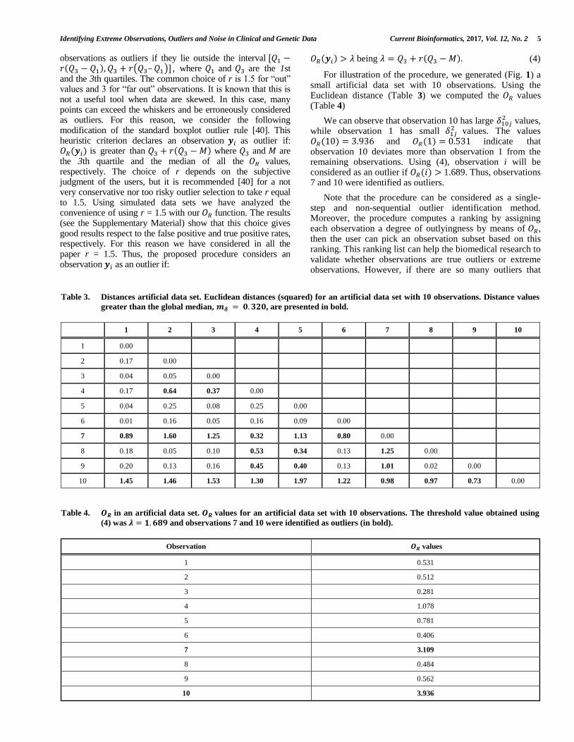
For illustration of the procedure, we generated (Fig. 1) a small artificial data set with 10 observations. Using the Euclidean distance (Table 3) we computed the 𝑂𝑅 values (Table 4)

We can observe that observation 10 has large 𝛿10𝑗2 values,

while observation 1 has small 𝛿1𝑗2 values. The values

𝑂𝑅(10) = 3.936 and 𝑂𝑅(1) = 0.531 indicate that observation 10 deviates more than observation 1 from the remaining observations. Using (4), observation i will be considered as an outlier if 𝑂𝑅(𝑖) > 1.689. Thus, observations 7 and 10 were identified as outliers.

Note that the procedure can be considered as a single-step and non-sequential outlier identification method. Moreover, the procedure computes a ranking by assigning each observation a degree of outlyingness by means of 𝑂𝑅, then the user can pick an observation subset based on this ranking. This ranking list can help the biomedical research to validate whether observations are true outliers or extreme observations. However, if there are so many outliers that

Table 3. Distances artificial data set. Euclidean distances (squared) for an artificial data set with 10 observations. Distance values

greater than the global median, 𝒎𝜹 = 𝟎. 𝟑𝟐𝟎, are presented in bold.

1 2 3 4 5 6 7 8 9 10

1 0.00

2 0.17 0.00

3 0.04 0.05 0.00

4 0.17 0.64 0.37 0.00

5 0.04 0.25 0.08 0.25 0.00

6 0.01 0.16 0.05 0.16 0.09 0.00

7 0.89 1.60 1.25 0.32 1.13 0.80 0.00

8 0.18 0.05 0.10 0.53 0.34 0.13 1.25 0.00

9 0.20 0.13 0.16 0.45 0.40 0.13 1.01 0.02 0.00

10 1.45 1.46 1.53 1.30 1.97 1.22 0.98 0.97 0.73 0.00

Table 4. 𝑶𝑹 in an artificial data set. 𝑶𝑹 values for an artificial data set with 10 observations. The threshold value obtained using

(4) was 𝝀 = 𝟏. 𝟔𝟖𝟗 and observations 7 and 10 were identified as outliers (in bold).

Observation 𝑶𝑹 values

1 0.531

2 0.512

3 0.281

4 1.078

5 0.781

6 0.406

7 3.109

8 0.484

9 0.562

10 3.936


individual inspection of each one is impossible, the cutoff rule (4) is needed. It is important to note that 𝑂𝑅 takes into account both, the relation of any observation with respect to the other observations in the data set and the dispersion of all data. Finally, it can be interpreted as the ratio of the variability around the observation and the variability around the center of the all data.

In the following, simulation studies and applications to actual data were used to empirically evaluate the proposed procedure.

3. RESULTS

3.1. Simulation Experiments

3.1.1. Masking Effect

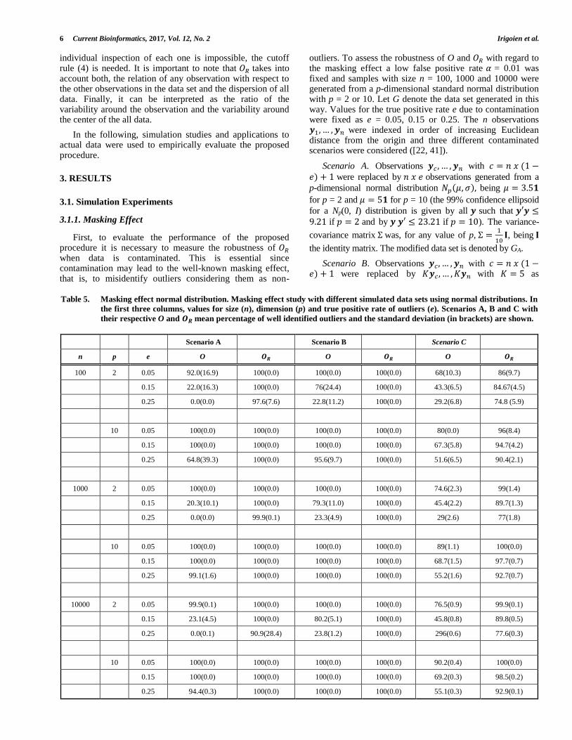
First, to evaluate the performance of the proposed procedure it is necessary to measure the robustness of 𝑂𝑅 when data is contaminated. This is essential since contamination may lead to the well-known masking effect, that is, to misidentify outliers considering them as non-

outliers. To assess the robustness of O and 𝑂𝑅 with regard to the masking effect a low false positive rate 𝛼 = 0.01 was fixed and samples with size n = 100, 1000 and 10000 were generated from a p-dimensional standard normal distribution with p = 2 or 10. Let G denote the data set generated in this way. Values for the true positive rate e due to contamination were fixed as e = 0.05, 0.15 or 0.25. The n observations 𝒚1, … , 𝒚𝑛 were indexed in order of increasing Euclidean distance from the origin and three different contaminated scenarios were considered ([22, 41]).

Scenario A. Observations 𝒚𝑐 , … , 𝒚𝑛 with 𝑐 = 𝑛 𝑥 (1 −𝑒) + 1 were replaced by 𝑛 𝑥 𝑒 observations generated from a

p-dimensional normal distribution 𝑁𝑝(𝜇, 𝜎), being 𝜇 = 3.5𝟏

for p = 2 and 𝜇 = 5𝟏 for p = 10 (the 99% confidence ellipsoid

for a Np(0, I) distribution is given by all 𝒚 such that 𝒚′𝒚 ≤9.21 if 𝑝 = 2 and by 𝒚 𝒚′ ≤ 23.21 if 𝑝 = 10). The variance-

covariance matrix Σ was, for any value of p, Σ =1

10𝐈, being 𝐈

the identity matrix. The modified data set is denoted by GA.

Scenario B. Observations 𝒚𝑐, … , 𝒚𝑛 with 𝑐 = 𝑛 𝑥 (1 −𝑒) + 1 were replaced by 𝐾𝒚𝑐, … , 𝐾𝒚𝑛 with 𝐾 = 5 as

Table 5. Masking effect normal distribution. Masking effect study with different simulated data sets using normal distributions. In

the first three columns, values for size (n), dimension (p) and true positive rate of outliers (e). Scenarios A, B and C with

their respective O and 𝑶𝑹 mean percentage of well identified outliers and the standard deviation (in brackets) are shown.

Scenario A Scenario B Scenario C

n p e O 𝑶𝑹 O 𝑶𝑹 O 𝑶𝑹

100 2 0.05 92.0(16.9) 100(0.0) 100(0.0) 100(0.0) 68(10.3) 86(9.7)

0.15 22.0(16.3) 100(0.0) 76(24.4) 100(0.0) 43.3(6.5) 84.67(4.5)

0.25 0.0(0.0) 97.6(7.6) 22.8(11.2) 100(0.0) 29.2(6.8) 74.8 (5.9)

10 0.05 100(0.0) 100(0.0) 100(0.0) 100(0.0) 80(0.0) 96(8.4)

0.15 100(0.0) 100(0.0) 100(0.0) 100(0.0) 67.3(5.8) 94.7(4.2)

0.25 64.8(39.3) 100(0.0) 95.6(9.7) 100(0.0) 51.6(6.5) 90.4(2.1)

1000 2 0.05 100(0.0) 100(0.0) 100(0.0) 100(0.0) 74.6(2.3) 99(1.4)

0.15 20.3(10.1) 100(0.0) 79.3(11.0) 100(0.0) 45.4(2.2) 89.7(1.3)

0.25 0.0(0.0) 99.9(0.1) 23.3(4.9) 100(0.0) 29(2.6) 77(1.8)

10 0.05 100(0.0) 100(0.0) 100(0.0) 100(0.0) 89(1.1) 100(0.0)

0.15 100(0.0) 100(0.0) 100(0.0) 100(0.0) 68.7(1.5) 97.7(0.7)

0.25 99.1(1.6) 100(0.0) 100(0.0) 100(0.0) 55.2(1.6) 92.7(0.7)

10000 2 0.05 99.9(0.1) 100(0.0) 100(0.0) 100(0.0) 76.5(0.9) 99.9(0.1)

0.15 23.1(4.5) 100(0.0) 80.2(5.1) 100(0.0) 45.8(0.8) 89.8(0.5)

0.25 0.0(0.1) 90.9(28.4) 23.8(1.2) 100(0.0) 296(0.6) 77.6(0.3)

10 0.05 100(0.0) 100(0.0) 100(0.0) 100(0.0) 90.2(0.4) 100(0.0)

0.15 100(0.0) 100(0.0) 100(0.0) 100(0.0) 69.2(0.3) 98.5(0.2)

0.25 94.4(0.3) 100(0.0) 100(0.0) 100(0.0) 55.1(0.3) 92.9(0.1)


inflation factor. Thus, outliers are along the ray in the direction of the replaced observations from the origin. Let GB denote the modified data set.

Scenario C. Observations 𝒚𝑐 , … , 𝒚𝑛 with 𝑐 = 𝑛 𝑥 (1 −𝑒) + 1 were replaced by 𝐾1𝒚𝑐, … , 𝐾𝑛𝑥𝑒𝒚𝑛 for same inflation factors, 𝐾1 = 1.25 and 𝐾𝑖 = 𝐾𝑖−1 + 3.5/(𝑛𝑥 𝑒 − 1) . Now

the outliers are in the direction of 𝒚𝑛 from the origin. Denote the modified data set by GC.

For the four data sets G, GA, GB and GC the Euclidean distance was used and we proceeded as follows. For observations in G, the non-contaminated case, the O and 𝑂𝑅 indices were calculated. As the false positive rate was fixed

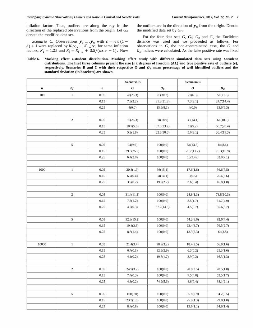
Table 6. Masking effect t-student distribution. Masking effect study with different simulated data sets using t-student

distributions. The first three columns present the size (n), degrees of freedom (d.f.) and true positive rate of outliers (e),

respectively. Scenarios B and C with their respective O and 𝑶𝑹 mean percentage of well identified outliers and the

standard deviation (in brackets) are shown.

Scenario B Scenario C

n d.f. e O 𝑶𝑹 O 𝑶𝑹

100 1 0.05 28(25.3) 70(30.2) 22(6.3) 50(21.6)

0.15 7.3(2.2) 31.3(21.8) 7.3(2.1) 24.7(14.4)

0.25 4(0.0) 15.6(8.1) 4(0.0) 13.6(6.3)

2 0.05 36(26.3) 94(18.9) 30(14.1) 66(18.9)

0.15 10.7(5.6) 87.3(23.2) 12(5.2) 50.7(20.4)

0.25 5.2(1.8) 62.8(38.6) 5.6(2.1) 36.4(19.3)

5 0.05 94(9.6) 100(0.0) 54(13.5) 84(8.4)

0.15 29.3(25.2) 100(0.0) 26.7(11.7) 75.3(10.9)

0.25 6.4(2.8) 100(0.0) 10(3.49) 52.8(7.1)

1000 1 0.05 20.8(1.9) 93(15.1) 17.6(1.6) 56.6(7.5)

0.15 6.7(0.4) 34(14.1) 6(0.5) 26.4(8.6)

0.25 3.9(0.2) 19.9(2.2) 3.6(0.4) 16.8(1.8)

2 0.05 31.4(11.1) 100(0.0) 24.8(1.3) 78.8(10.3)

0.15 7.8(1.2) 100(0.0) 8.5(1.7) 51.7(4.9)

0.25 4.2(0.3) 67.2(14.5) 4.5(0.7) 35.6(3.7)

5 0.05 92.8(15.2) 100(0.0) 54.2(8.6) 92.6(4.4)

0.15 19.4(3.8) 100(0.0) 22.4(3.7) 76.5(2.7)

0.25 8.6(1.4) 100(0.0) 13.9(2.3) 64(3.8)

10000 1 0.05 21.4(3.4) 98.9(3.2) 18.4(2.5) 56.8(1.6)

0.15 6.7(0.1) 32.8(2.9) 6.3(0.2) 25.3(1.6)

0.25 4.1(0.2) 19.5(1.7) 3.9(0.2) 16.3(1.3)

2 0.05 24.9(3.2) 100(0.0) 20.8(2.5) 78.5(1.8)

0.15 7.4(0.3) 100(0.0) 7.5(4.8) 52.5(1.7)

0.25 4.3(0.2) 74.2(5.6) 4.6(0.4) 38.1(2.1)

5 0.05 100(0.0) 100(0.0) 55.8(0.9) 94.2(0.5)

0.15 23.3(1.8) 100(0.0) 25.9(1.3) 79.8(1.0)

0.25 8.4(0.8) 100(0.0) 13.9(1.1) 64.6(1.4)


at 𝛼 = 0.01, the 𝑛x𝛼-th largest value will serve as a threshold value for outlier detection under scenarios A, B and C. For each scenario and for each value of n, p and e, ten data sets were generated. We find (Table 5), that the outlier identifier 𝑂𝑅 outperforms for all situations. The 𝑂𝑅 identifier almost detected all outliers under scenario A; under scenario B it obtained excellent results identifying all outliers while in Scenario C only the most extreme cases were detected. This is not surprising by the construction of the modified data set GC and by identification of outliers at a single step. However, under Scenario C and when dimensionality increases, 𝑂𝑅 tends to perform much better identifying almost all outliers.

In order to study the robustness when the features follow distributions with heaver tails, we also considered the t-distribution with small degrees of freedom. Thus, for the same false positive rate 𝛼 = 0.01, samples with size 𝑛 =100, 1000 and 10000 were generated from a 2-dimensional distribution, with any marginal following a t-student with 𝜈 = 1, 2 and 5 degrees of freedom. That is, we used the 2-dimensional t-Student distribution given by 𝑇𝑀2(𝜇, Σ, 𝑛) =Γ(𝜈 + 2 2⁄ )(𝜋𝜈)−1Γ(𝜈 2⁄ )−1𝑑𝑒𝑡(Σ)−1 2⁄ [1 + (𝒚 −𝜇)′Σ−1(𝒚 − 𝜇)/𝜈]−(𝜈+2)/2 , being Γ the Gamma function, 𝜇 = (0,0) , Σ = 𝐈 and 𝜈 = 1, 2 , and 5, respectively. As before, values for the true positive rate e due to contamination were fixed as 𝑒 = 0.05, 0.15 or 0.25 and contaminated scenarios B and C were considered. For each scenario and for each value of n, e and degrees of freedom, ten data sets were generated. As we can observe in Table 6, under scenario B better results were found and the outlier identifier 𝑂𝑅 is, in all cases, more robust than O.

3.1.2 Noise Detection

In order to explore the efficiency of the procedure in front of noise, we provide the following microarray study. Using a

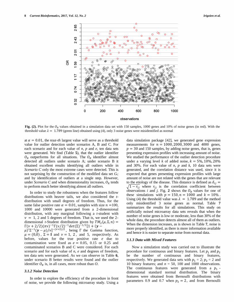
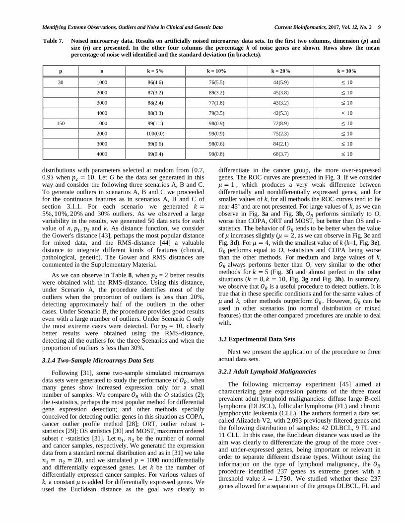
data simulation package [42], we generated gene expression measurements for 𝑛 = 1000, 2000, 3000 and 4000 genes, 𝑝 = 30 and 150 samples, by adding noise genes, that is, genes presenting expression profiles with increasing amount of noise. We studied the performance of the outlier detection procedure under a varying level k of added noise, 𝑘 = 5%, 10%, 20% and 30%. For each value of n, p and k, 10 data sets were generated, and the correlation distance was used, since it is expected that genes presenting expression profiles with large amount of noise are not related with the genes that are relevant to the etiology of the disease. This distance is defined as 𝛿𝑖𝑗 =√1 − 𝑟𝑖𝑗 where 𝑟𝑖𝑗 is the correlation coefficient between observations i and j. Fig. 2 shows the 𝑂𝑅 values for one of these simulations with 𝑝 = 150, 𝑛 = 1000 and 𝑘 = 10% . Using (4) the threshold value was 𝜆 = 1.789 and the method only misidentified 3 noise genes as normal. Table 7 summarizes the results for all simulations. This study on artificially noised microarray data sets reveals that when the number of noise genes is low or moderate, less than 30% of the whole data, the procedure detects almost all of them as outliers. When the dimension increases, as is shown in Table 7, noise is more properly identified, as there is more information available and hence it is easier to separate noise from normal data.

3.1.3 Data with Mixed Features

Now a simulation study was carried out to illustrate the procedure for continuous and binary features. Let 𝑝1 and 𝑝2 be the number of continuous and binary features, respectively. We generated data sets with 𝑝1 = 2; 𝑝2 = 2 and 10 binary features; and n = 50, 100 and 1000 observations. The continuous features were generated from a 𝑝1 -dimensional standard normal distribution. The binary features were obtained from Bernoulli distributions with parameters 0.9 and 0.7 when 𝑝2 = 2 , and from Bernoulli

Fig. (2). Plot for the 𝑂𝑅 values obtained in a simulation data set with 150 samples, 1000 genes and 10% of noise genes (in red). With the

threshold value 𝜆 = 1.789 (green line) obtained using (4), only 3 noise genes were misidentified as normal


distributions with parameters selected at random from {0.7, 0.9} when 𝑝2 = 10. Let G be the data set generated in this way and consider the following three scenarios A, B and C. To generate outliers in scenarios A, B and C we proceeded for the continuous features as in scenarios A, B and C of section 3.1.1. For each scenario we generated 𝑘 =5%, 10%, 20% and 30% outliers. As we observed a large variability in the results, we generated 50 data sets for each value of n, 𝑝1, 𝑝2 and k. As distance function, we consider the Gower's distance [43], perhaps the most popular distance for mixed data, and the RMS-distance [44] a valuable distance to integrate different kinds of features (clinical, pathological, genetic). The Gower and RMS distances are commented in the Supplementary Material.

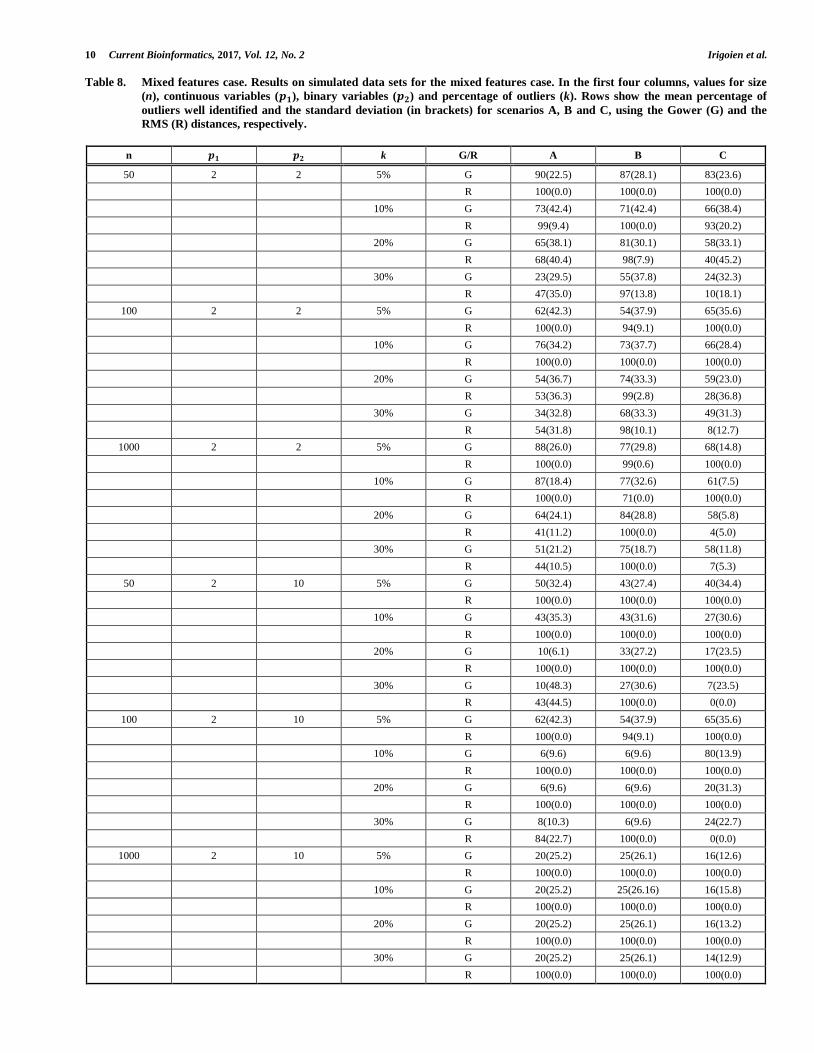
As we can observe in Table 8, when 𝑝2 = 2 better results were obtained with the RMS-distance. Using this distance, under Scenario A, the procedure identifies most of the outliers when the proportion of outliers is less than 20%, detecting approximately half of the outliers in the other cases. Under Scenario B, the procedure provides good results even with a large number of outliers. Under Scenario C only the most extreme cases were detected. For 𝑝2 = 10, clearly better results were obtained using the RMS-distance, detecting all the outliers for the three Scenarios and when the proportion of outliers is less than 30%.

3.1.4 Two-Sample Microarrays Data Sets

Following [31], some two-sample simulated microarrays data sets were generated to study the performance of 𝑂𝑅 , when many genes show increased expression only for a small number of samples. We compare 𝑂𝑅 with the O statistics (2); the t-statistics, perhaps the most popular method for differential gene expression detection; and other methods specially conceived for detecting outlier genes in this situation as COPA, cancer outlier profile method [28]; ORT, outlier robust t-statistics [29]; OS statistics [30] and MOST, maximum ordered subset t -statistics [31]. Let 𝑛1, 𝑛2 be the number of normal and cancer samples, respectively. We generated the expression data from a standard normal distribution and as in [31] we take 𝑛1 = 𝑛2 = 20, and we simulated p = 1000 nondifferentially and differentially expressed genes. Let k be the number of differentially expressed cancer samples. For various values of k, a constant 𝜇 is added for differentially expressed genes. We used the Euclidean distance as the goal was clearly to

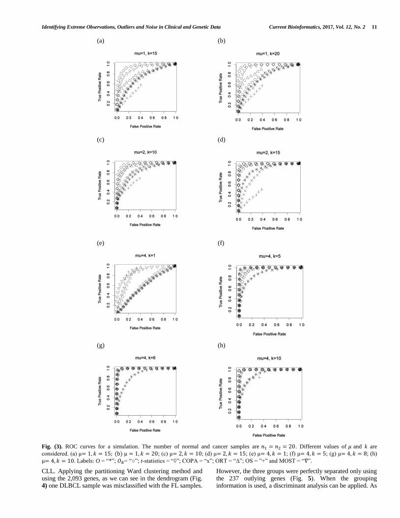
differentiate in the cancer group, the more over-expressed genes. The ROC curves are presented in Fig. 3. If we consider 𝜇 = 1 , which produces a very weak difference between differentially and nondifferentially expressed genes, and for smaller values of k, for all methods the ROC curves tend to lie near 45º and are not presented. For large values of k, as we can observe in Fig. 3a and Fig. 3b, 𝑂𝑅 performs similarly to O, worse than COPA, ORT and MOST, but better than OS and t-statistics. The behavior of 𝑂𝑅 tends to be better when the value of 𝜇 increases slightly (𝜇 = 2, as we can observe in Fig. 3c and Fig. 3d). For 𝜇 = 4, with the smallest value of k (k=1, Fig. 3e), 𝑂𝑅 performs equal to O, t-statistics and COPA being worse than the other methods. For medium and large values of k, 𝑂𝑅 always performs better than O, very similar to the other methods for 𝑘 = 5 (Fig. 3f) and almost perfect in the other situations (𝑘 = 8, 𝑘 = 10, Fig. 3g and Fig. 3h). In summary, we observe that 𝑂𝑅 is a useful procedure to detect outliers. It is true that in these specific conditions and for the same values of 𝜇 and k, other methods outperform 𝑂𝑅 . However, 𝑂𝑅 can be used in other scenarios (no normal distribution or mixed features) that the other compared procedures are unable to deal with.

3.2 Experimental Data Sets

Next we present the application of the procedure to three actual data sets.

3.2.1 Adult Lymphoid Malignancies

The following microarray experiment [45] aimed at characterizing gene expression patterns of the three most prevalent adult lymphoid malignancies: diffuse large B-cell lymphoma (DLBCL), follicular lymphoma (FL) and chronic lymphocytic leukemia (CLL). The authors formed a data set, called Alizadeh-V2, with 2,093 previously filtered genes and the following distribution of samples: 42 DLBCL, 9 FL and 11 CLL. In this case, the Euclidean distance was used as the aim was clearly to differentiate the group of the more over- and under-expressed genes, being important or relevant in order to separate different disease types. Without using the information on the type of lymphoid malignancy, the 𝑂𝑅 procedure identified 237 genes as extreme genes with a threshold value 𝜆 = 1.750. We studied whether these 237 genes allowed for a separation of the groups DLBCL, FL and

Table 7. Noised microarray data. Results on artificially noised microarray data sets. In the first two columns, dimension (p) and

size (n) are presented. In the other four columns the percentage k of noise genes are shown. Rows show the mean

percentage of noise well identified and the standard deviation (in brackets).

p n k = 5% k = 10% k = 20% k = 30%

30 1000 86(4.6) 76(5.5) 44(5.9) ≤ 10

2000 87(3.2) 89(3.2) 45(3.8) ≤ 10

3000 88(2.4) 77(1.8) 43(3.2) ≤ 10

4000 88(3.3) 79(3.5) 42(5.3) ≤ 10

150 1000 99(1.1) 98(0.9) 72(8.9) ≤ 10

2000 100(0.0) 99(0.9) 75(2.3) ≤ 10

3000 99(0.6) 98(0.6) 84(2.1) ≤ 10

4000 99(0.4) 99(0.8) 68(3.7) ≤ 10


Table 8. Mixed features case. Results on simulated data sets for the mixed features case. In the first four columns, values for size

(n), continuous variables (𝒑𝟏), binary variables (𝒑𝟐) and percentage of outliers (k). Rows show the mean percentage of

outliers well identified and the standard deviation (in brackets) for scenarios A, B and C, using the Gower (G) and the

RMS (R) distances, respectively.

n 𝒑𝟏 𝒑𝟐 k G/R A B C

50 2 2 5% G 90(22.5) 87(28.1) 83(23.6)

R 100(0.0) 100(0.0) 100(0.0)

10% G 73(42.4) 71(42.4) 66(38.4)

R 99(9.4) 100(0.0) 93(20.2)

20% G 65(38.1) 81(30.1) 58(33.1)

R 68(40.4) 98(7.9) 40(45.2)

30% G 23(29.5) 55(37.8) 24(32.3)

R 47(35.0) 97(13.8) 10(18.1)

100 2 2 5% G 62(42.3) 54(37.9) 65(35.6)

R 100(0.0) 94(9.1) 100(0.0)

10% G 76(34.2) 73(37.7) 66(28.4)

R 100(0.0) 100(0.0) 100(0.0)

20% G 54(36.7) 74(33.3) 59(23.0)

R 53(36.3) 99(2.8) 28(36.8)

30% G 34(32.8) 68(33.3) 49(31.3)

R 54(31.8) 98(10.1) 8(12.7)

1000 2 2 5% G 88(26.0) 77(29.8) 68(14.8)

R 100(0.0) 99(0.6) 100(0.0)

10% G 87(18.4) 77(32.6) 61(7.5)

R 100(0.0) 71(0.0) 100(0.0)

20% G 64(24.1) 84(28.8) 58(5.8)

R 41(11.2) 100(0.0) 4(5.0)

30% G 51(21.2) 75(18.7) 58(11.8)

R 44(10.5) 100(0.0) 7(5.3)

50 2 10 5% G 50(32.4) 43(27.4) 40(34.4)

R 100(0.0) 100(0.0) 100(0.0)

10% G 43(35.3) 43(31.6) 27(30.6)

R 100(0.0) 100(0.0) 100(0.0)

20% G 10(6.1) 33(27.2) 17(23.5)

R 100(0.0) 100(0.0) 100(0.0)

30% G 10(48.3) 27(30.6) 7(23.5)

R 43(44.5) 100(0.0) 0(0.0)

100 2 10 5% G 62(42.3) 54(37.9) 65(35.6)

R 100(0.0) 94(9.1) 100(0.0)

10% G 6(9.6) 6(9.6) 80(13.9)

R 100(0.0) 100(0.0) 100(0.0)

20% G 6(9.6) 6(9.6) 20(31.3)

R 100(0.0) 100(0.0) 100(0.0)

30% G 8(10.3) 6(9.6) 24(22.7)

R 84(22.7) 100(0.0) 0(0.0)

1000 2 10 5% G 20(25.2) 25(26.1) 16(12.6)

R 100(0.0) 100(0.0) 100(0.0)

10% G 20(25.2) 25(26.16) 16(15.8)

R 100(0.0) 100(0.0) 100(0.0)

20% G 20(25.2) 25(26.1) 16(13.2)

R 100(0.0) 100(0.0) 100(0.0)

30% G 20(25.2) 25(26.1) 14(12.9)

R 100(0.0) 100(0.0) 100(0.0)


(a)

(b)

(c)

(d)

(e)

(f)

(g)

(h)

Fig. (3). ROC curves for a simulation. The number of normal and cancer samples are 𝑛1 = 𝑛2 = 20. Different values of 𝜇 and k are

considered. (a) μ= 1, 𝑘 = 15; (b) μ = 1, 𝑘 = 20; (c) μ= 2, 𝑘 = 10; (d) μ= 2, 𝑘 = 15; (e) μ= 4, 𝑘 = 1; (f) μ= 4, 𝑘 = 5; (g) μ= 4, 𝑘 = 8; (h)

μ= 4, 𝑘 = 10. Labels: O = “*”; 𝑂𝑅= “○”; t-statistics = “◊”; COPA = “x”; ORT = “∆”; OS = ”+” and MOST = “∇”.

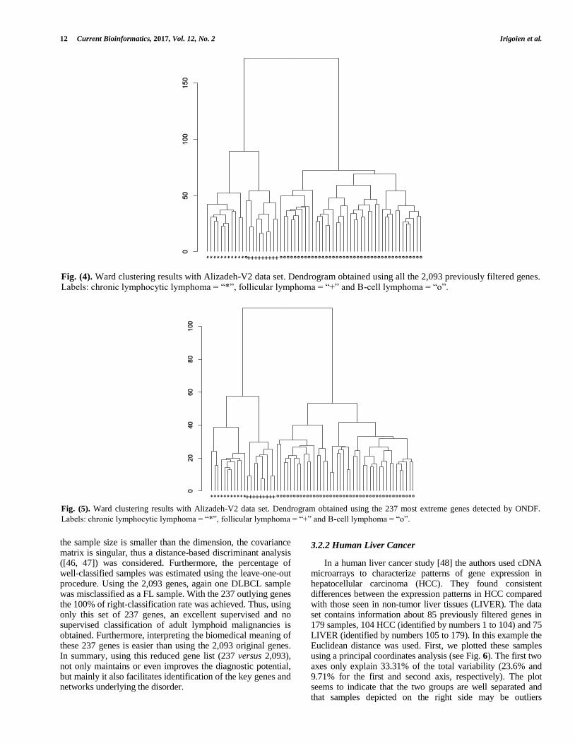
CLL. Applying the partitioning Ward clustering method and using the 2,093 genes, as we can see in the dendrogram (Fig. 4) one DLBCL sample was misclassified with the FL samples.

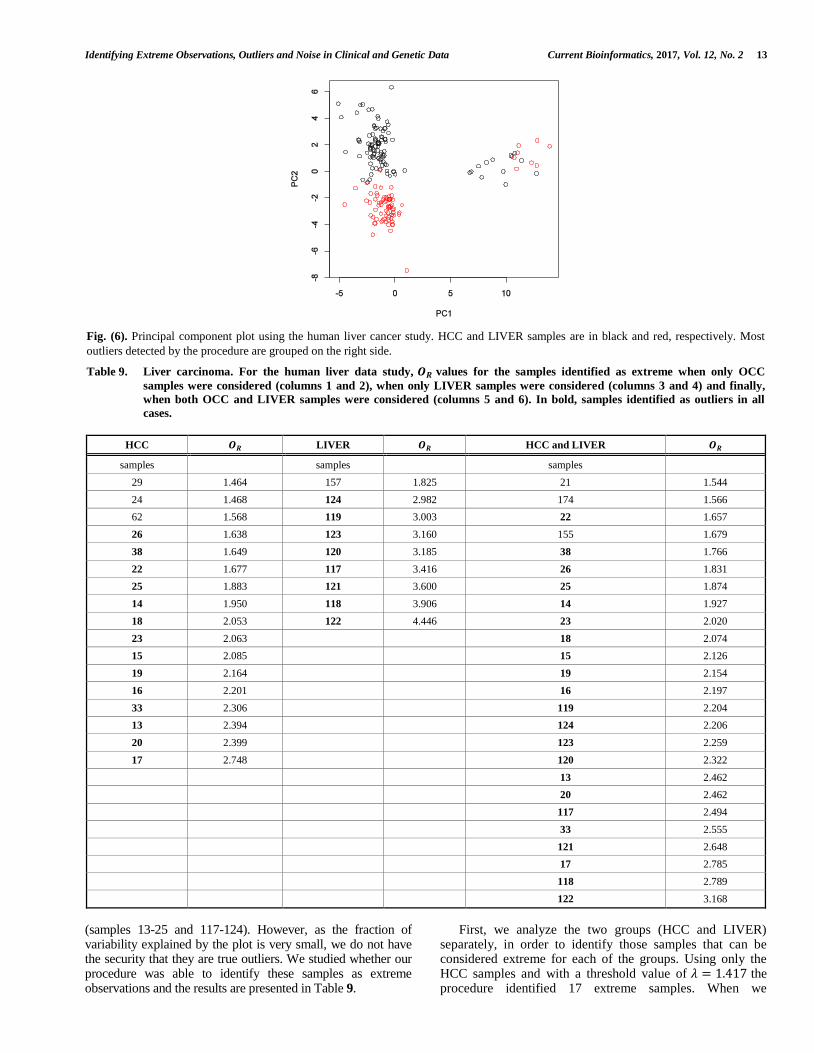
However, the three groups were perfectly separated only using the 237 outlying genes (Fig. 5). When the grouping information is used, a discriminant analysis can be applied. As


the sample size is smaller than the dimension, the covariance matrix is singular, thus a distance-based discriminant analysis ([46, 47]) was considered. Furthermore, the percentage of well-classified samples was estimated using the leave-one-out procedure. Using the 2,093 genes, again one DLBCL sample was misclassified as a FL sample. With the 237 outlying genes the 100% of right-classification rate was achieved. Thus, using only this set of 237 genes, an excellent supervised and no supervised classification of adult lymphoid malignancies is obtained. Furthermore, interpreting the biomedical meaning of these 237 genes is easier than using the 2,093 original genes. In summary, using this reduced gene list (237 versus 2,093), not only maintains or even improves the diagnostic potential, but mainly it also facilitates identification of the key genes and networks underlying the disorder.

3.2.2 Human Liver Cancer

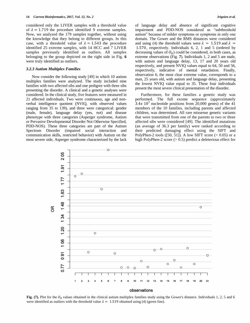
In a human liver cancer study [48] the authors used cDNA microarrays to characterize patterns of gene expression in hepatocellular carcinoma (HCC). They found consistent differences between the expression patterns in HCC compared with those seen in non-tumor liver tissues (LIVER). The data set contains information about 85 previously filtered genes in 179 samples, 104 HCC (identified by numbers 1 to 104) and 75 LIVER (identified by numbers 105 to 179). In this example the Euclidean distance was used. First, we plotted these samples using a principal coordinates analysis (see Fig. 6). The first two axes only explain 33.31% of the total variability (23.6% and 9.71% for the first and second axis, respectively). The plot seems to indicate that the two groups are well separated and that samples depicted on the right side may be outliers

Fig. (4). Ward clustering results with Alizadeh-V2 data set. Dendrogram obtained using all the 2,093 previously filtered genes. Labels: chronic lymphocytic lymphoma = “*”, follicular lymphoma = “+” and B-cell lymphoma = “o”.

Fig. (5). Ward clustering results with Alizadeh-V2 data set. Dendrogram obtained using the 237 most extreme genes detected by ONDF.

Labels: chronic lymphocytic lymphoma = “*”, follicular lymphoma = “+” and B-cell lymphoma = “o”.


(samples 13-25 and 117-124). However, as the fraction of variability explained by the plot is very small, we do not have the security that they are true outliers. We studied whether our procedure was able to identify these samples as extreme observations and the results are presented in Table 9.

First, we analyze the two groups (HCC and LIVER) separately, in order to identify those samples that can be considered extreme for each of the groups. Using only the HCC samples and with a threshold value of 𝜆 = 1.417 the procedure identified 17 extreme samples. When we

Fig. (6). Principal component plot using the human liver cancer study. HCC and LIVER samples are in black and red, respectively. Most

outliers detected by the procedure are grouped on the right side.

Table 9. Liver carcinoma. For the human liver data study, 𝑶𝑹 values for the samples identified as extreme when only OCC

samples were considered (columns 1 and 2), when only LIVER samples were considered (columns 3 and 4) and finally,

when both OCC and LIVER samples were considered (columns 5 and 6). In bold, samples identified as outliers in all

cases.

HCC 𝑶𝑹 LIVER 𝑶𝑹 HCC and LIVER 𝑶𝑹

samples samples samples

29 1.464 157 1.825 21 1.544

24 1.468 124 2.982 174 1.566

62 1.568 119 3.003 22 1.657

26 1.638 123 3.160 155 1.679

38 1.649 120 3.185 38 1.766

22 1.677 117 3.416 26 1.831

25 1.883 121 3.600 25 1.874

14 1.950 118 3.906 14 1.927

18 2.053 122 4.446 23 2.020

23 2.063 18 2.074

15 2.085 15 2.126

19 2.164 19 2.154

16 2.201 16 2.197

33 2.306 119 2.204

13 2.394 124 2.206

20 2.399 123 2.259

17 2.748 120 2.322

13 2.462

20 2.462

117 2.494

33 2.555

121 2.648

17 2.785

118 2.789

122 3.168


considered only the LIVER samples with a threshold value of 𝜆 = 1.719 the procedure identified 9 extreme samples. Now, we analyzed the 179 samples together, without using the knowledge that they belong to different groups. In this case, with a threshold value of 𝜆 = 1.543 the procedure identified 25 extreme samples, with 14 HCC and 7 LIVER samples previously identified as outliers. All samples belonging to the group depicted on the right side in Fig. 6 were truly identified as outliers.

3.2.3 Autism Multiplex Families

Now consider the following study [49] in which 10 autism multiplex families were analyzed. The study included nine families with two affected sibs and one pedigree with three sibs presenting the disorder. A clinical and a genetic analyses were considered. In the clinical study, five features were measured in 21 affected individuals. Two were continuous, age and non-verbal intelligence quotient (NVIQ, with observed values ranging from 35 to 139), and three were categorical: gender (male, female), language delay (yes, not) and disease phenotype with three categories (Asperger syndrome, Autism or Pervasive Developmental Disorder Not Otherwise Specified, PDD-NOS). These three categories are part of the Autism Spectrum Disorder (impaired social interaction and communication skills, restricted behavior) with Autism on the most severe side, Asperger syndrome characterized by the lack

of language delay and absence of significant cognitive impairment and PDD-NOS considered as “subthreshold autism” because of milder symptoms or symptoms in only one domain. The Gower and the RMS distances were considered and using (4) the threshold values were 𝜆 = 1.519 and 𝜆 = 1.570 , respectively. Individuals 6, 2, 1 and 5 (ordered by decreasing values of 𝑂𝑅) could be considered, in both cases, as extreme observations (Fig. 7). Individuals 1, 2 and 5 are male, with autism and language delay, 13, 17 and 20 years old respectively, and present NVIQ values equal to 64, 50 and 56, respectively, indicative of mental retardation. Finally, observation 6, the most clear extreme value, corresponds to a man, 25 years old, with autism and language delay, presenting the lowest NVIQ value equal to 35. These four individuals present the most severe clinical presentation of the disorder.

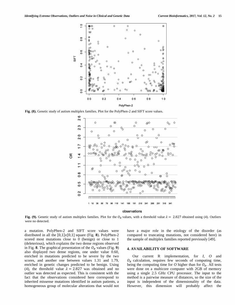
Furthermore, for these families a genetic study was performed. The full exome sequence (approximately 3.4𝑥 107 nucleotide positions from 20,000 genes) of the 41 members of the 10 families, including parents and affected children, was determined. All rare missense genetic variants that were transmitted from one of the parents to two or three affected sibs were considered [49]. The identified mutations (an average of 36.3 per family) were ranked according to their predicted damaging effect using the SIFT and PolyPhen-2 tools ([50, 51]). A low SIFT score (< 0.05) or a high PolyPhen-2 score (> 0.5) predict a deleterious effect for

Fig. (7). Plot for the 𝑂𝑅 values obtained in the clinical autism multiplex families study using the Gower's distance. Individuals 1, 2, 5 and 6

were identified as outliers with the threshold value 𝜆 = 1.519 obtained using (4) (green line).


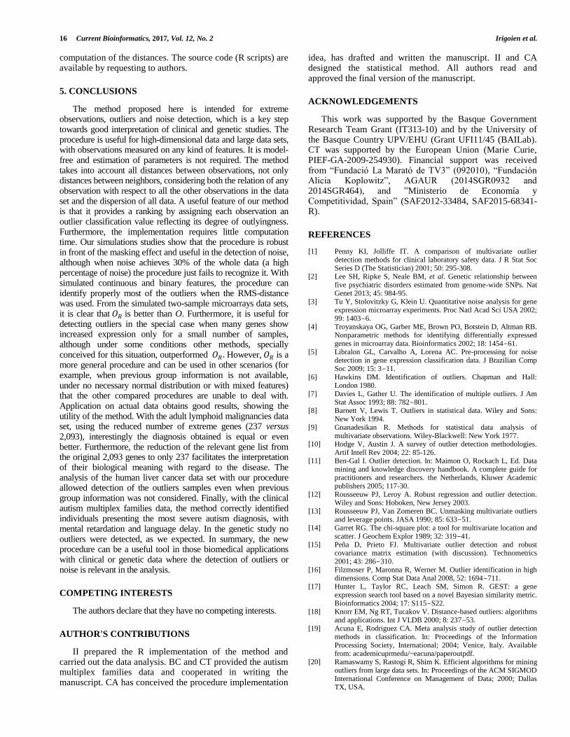
a mutation. PolyPhen-2 and SIFT score values were distributed in all the [0,1]𝑥[0,1] square (Fig. 8). PolyPhen-2 scored most mutations close to 0 (benign) or close to 1 (deleterious), which explains the two dense regions observed in Fig. 8. The graphical presentation of the 𝑂𝑅 values (Fig. 9) also displayed two dense regions, one under value 0.60, enriched in mutations predicted to be severe by the two scores, and another one between values 1.31 and 1.79, enriched in genetic changes predicted to be benign. Using (4), the threshold value 𝜆 = 2.827 was obtained and no outlier was detected as expected. This is consistent with the fact that the observations considered here correspond to inherited missense mutations identified in autism patients, a homogeneous group of molecular alterations that would not

have a major role in the etiology of the disorder (as compared to truncating mutations, not considered here) in the sample of multiplex families reported previously [49].

4. AVAILABILITY OF SOFTWARE

Our current R implementation, for I, O and 𝑂𝑅 calculation, requires few seconds of computing time, being the computing time for O higher than for 𝑂𝑅. All tests were done on a multicore computer with 2GB of memory using a single 2.5 GHz CPU processor. The input to the method is a pairwise measure of distances, so the size of the input is independent of the dimensionality of the data. However, this dimension will probably affect the

Fig. (8). Genetic study of autism multiplex families. Plot for the PolyPhen-2 and SIFT score values.

Fig. (9). Genetic study of autism multiplex families. Plot for the 𝑂𝑅 values, with a threshold value 𝜆 = 2.827 obtained using (4). Outliers

were no detected.


computation of the distances. The source code (R scripts) are available by requesting to authors.

5. CONCLUSIONS

The method proposed here is intended for extreme observations, outliers and noise detection, which is a key step towards good interpretation of clinical and genetic studies. The procedure is useful for high-dimensional data and large data sets, with observations measured on any kind of features. It is model-free and estimation of parameters is not required. The method takes into account all distances between observations, not only distances between neighbors, considering both the relation of any observation with respect to all the other observations in the data set and the dispersion of all data. A useful feature of our method is that it provides a ranking by assigning each observation an outlier classification value reflecting its degree of outlyingness. Furthermore, the implementation requires little computation time. Our simulations studies show that the procedure is robust in front of the masking effect and useful in the detection of noise, although when noise achieves 30% of the whole data (a high percentage of noise) the procedure just fails to recognize it. With simulated continuous and binary features, the procedure can identify properly most of the outliers when the RMS-distance was used. From the simulated two-sample microarrays data sets, it is clear that 𝑂𝑅 is better than O. Furthermore, it is useful for detecting outliers in the special case when many genes show increased expression only for a small number of samples, although under some conditions other methods, specially conceived for this situation, outperformed 𝑂𝑅 . However, 𝑂𝑅 is a more general procedure and can be used in other scenarios (for example, when previous group information is not available, under no necessary normal distribution or with mixed features) that the other compared procedures are unable to deal with. Application on actual data obtains good results, showing the utility of the method. With the adult lymphoid malignancies data set, using the reduced number of extreme genes (237 versus 2,093), interestingly the diagnosis obtained is equal or even better. Furthermore, the reduction of the relevant gene list from the original 2,093 genes to only 237 facilitates the interpretation of their biological meaning with regard to the disease. The analysis of the human liver cancer data set with our procedure allowed detection of the outliers samples even when previous group information was not considered. Finally, with the clinical autism multiplex families data, the method correctly identified individuals presenting the most severe autism diagnosis, with mental retardation and language delay. In the genetic study no outliers were detected, as we expected. In summary, the new procedure can be a useful tool in those biomedical applications with clinical or genetic data where the detection of outliers or noise is relevant in the analysis.

COMPETING INTERESTS

The authors declare that they have no competing interests.

AUTHOR'S CONTRIBUTIONS

II prepared the R implementation of the method and carried out the data analysis. BC and CT provided the autism multiplex families data and cooperated in writing the manuscript. CA has conceived the procedure implementation

idea, has drafted and written the manuscript. II and CA designed the statistical method. All authors read and approved the final version of the manuscript.

ACKNOWLEDGEMENTS

This work was supported by the Basque Government Research Team Grant (IT313-10) and by the University of the Basque Country UPV/EHU (Grant UFI11/45 (BAILab). CT was supported by the European Union (Marie Curie, PIEF-GA-2009-254930). Financial support was received from “Fundació La Marató de TV3” (092010), “Fundación Alicia Koplowitz”, AGAUR (2014SGR0932 and 2014SGR464), and ”Ministerio de Economía y Competitividad, Spain” (SAF2012-33484, SAF2015-68341-R).

REFERENCES

[1] Penny KI, Jolliffe IT. A comparison of multivariate outlier detection methods for clinical laboratory safety data. J R Stat Soc Series D (The Statistician) 2001; 50: 295-308.

[2] Lee SH, Ripke S, Neale BM, et al. Genetic relationship between five psychiatric disorders estimated from genome-wide SNPs. Nat Genet 2013; 45: 984-95.

[3] Tu Y, Stolovitzky G, Klein U. Quantitative noise analysis for gene expression microarray experiments. Proc Natl Acad Sci USA 2002; 99: 1403-6.

[4] Troyanskaya OG, Garber ME, Brown PO, Botstein D, Altman RB. Nonparametric methods for identifying differentially expressed genes in microarray data. Bioinformatics 2002; 18: 1454-61.

[5] Libralon GL, Carvalho A, Lorena AC. Pre-processing for noise detection in gene expression classification data. J Brazilian Comp Soc 2009; 15: 3-11.

[6] Hawkins DM. Identification of outliers. Chapman and Hall: London 1980.

[7] Davies L, Gather U. The identification of multiple outliers. J Am Stat Assoc 1993; 88: 782-801.

[8] Barnett V, Lewis T. Outliers in statistical data. Wiley and Sons: New York 1994.

[9] Gnanadesikan R. Methods for statistical data analysis of multivariate observations. Wiley-Blackwell: New York 1977.

[10] Hodge V, Austin J. A survey of outlier detection methodologies. Artif Intell Rev 2004; 22: 85-126.

[11] Ben-Gal I. Outlier detection. In: Maimon O, Rockach L, Ed. Data mining and knowledge discovery handbook. A complete guide for practitioners and researchers. the Netherlands, Kluwer Academic publishers 2005; 117-30.

[12] Rousseeuw PJ, Leroy A. Robust regression and outlier detection. Wiley and Sons: Hoboken, New Jersey 2003.

[13] Rousseeuw PJ, Van Zomeren BC. Unmasking multivariate outliers and leverage points. JASA 1990; 85: 633-51.

[14] Garret RG. The chi-square plot: a tool for multivariate location and scatter. J Geochem Explor 1989; 32: 319-41.

[15] Peña D, Prieto FJ. Multivariate outlier detection and robust covariance matrix estimation (with discussion). Technometrics 2001; 43: 286-310.

[16] Filzmoser P, Maronna R, Werner M. Outlier identification in high dimensions. Comp Stat Data Anal 2008, 52: 1694-711.

[17] Hunter L, Taylor RC, Leach SM, Simon R. GEST: a gene expression search tool based on a novel Bayesian similarity metric. Bioinformatics 2004; 17: S115-S22.

[18] Knorr EM, Ng RT, Tucakov V. Distance-based outliers: algorithms and applications. Int J VLDB 2000; 8: 237-53.

[19] Acuna E, Rodriguez CA. Meta analysis study of outlier detection methods in classification. In: Proceedings of the Information Processing Society, International; 2004; Venice, Italy. Available from: academicuprmedu/~eacuna/paperoutpdf.

[20] Ramaswamy S, Rastogi R, Shim K. Efficient algorithms for mining outliers from large data sets. In: Proceedings of the ACM SIGMOD International Conference on Management of Data; 2000; Dallas TX, USA.


[21] Chen Y, Dang X, Peng H, Bart HL. Outlier detection with the kernelized spatial depth function. IEEE T Pattern Anal 2009; 31: 288-305.

[22] Dang X, Serfling R. Nonparametric depth multivariate outlier identifiers and masking robustness properties. J Stat Plan and Infer 2010; 140: 198-213.

[23] Liu RY. On a notion of data depth based on random simplices. Ann Statist 1990; 18: 405-14.

[24] Vardi Y, Zhang C. The multivariate L1-median and associated data depth. Proc Natl Acad Sci USA 2000; 97: 1423-6.

[25] Zuo S, Serfling R. General notions of statistical depth function. Ann Statist 2000; 28: 461-82.

[26] Serfling R. A depth function and a scale curve based on spatial quantiles. In: Dodge Y, Ed. Statistic and Data Analysis Based on L1-Norm and Related Methods. Boston, Birkhauser 2002; 25-38.

[27] Irigoien I, Mestres F, Arenas C. The depth problem: identifying the most representative units in a data group. IEEE ACM T Comput Bi 2013; 10: 161-72.

[28] Tomlins SA, Rhodes DR, Perne S, et al. Recurrent fusion of TMPRSS2 and ETS transcription factor genes in prostate cancer. Science 2005; 310: 644-8.

[29] Wu B. Cancer outlier differential gene expression detection. Biostatistics 2007; 8: 566-75.

[30] Tibshirani R, Hastie T. Outlier sums for differential gene expression analysis. Biostatistics 2007; 8: 2-8.

[31] Lian H. MOST: detecting cancer differential gene expression. Biostatistics 2008; 9: 411-8.

[32] Ghosh D. Genomic outlier profile analysis: mixture models null hypotheses and nonparametric estimation. Biostatistics 2009; 10: 60-9.

[33] Cuadras CM, Fortiana J. A continuous metric scaling solution for a random variable. J Multivariate Anal 1995; 32: 1-14.

[34] Rao CR. Diversity: its measurement decomposition apportionment and analysis. Sankhya Indian J Stat 1982; 44: 1-22.

[35] Arenas C, Cuadras CM. Some recent statistical methods based on distances. Contri Sci 2002; 2: 183-91.

[36] Irigoien I, Arenas C. INCA: new statistics for estimating the number of clusters and identifying atypical units. Stat Med 2008; 27: 2948-73.

[37] Irigoien I, Sierra B, Arenas C. ICGE: an R package for detecting relevant clusters and atypical units in gene expression. BMC Bioinformatics 2013; 13: 30-41.

[38] Maronna RA, Martin RD, Yohai VJ. Robust Statistics. Theory and Methods. John Wiley and Sons, England; 2006.

[39] Tuckey JW. Exploratory data analysis. Addison-Wesley: New York 1977.

[40] Kimber AC. Exploratory data analysis for possibly censored data from skewed distributions. Appl Statist 1990; 39: 21-30.

[41] Filzmoser P. A multivariate outlier detection method. Proceedings of the Seventh International Conference on Computer Analysis and Modeling; 2004; Minsk, Belarus.

[42] Langfelder P, Horvath S. Eingene networks for studying the relationships between co-expression modules. BMC Syst Biol 2007; 1: 1-54.

[43] Gower JC. A general coefficient of similarity and some of its properties. Biometrics 1971; 27: 857-71.

[44] Irigoien I, Arenas C. Diagnosis using clinical/pathological and molecular information. Stat Methods Med Res 2014; DOI: 101177-0962280214534410.

[45] Alizadeh AA, Eisen MB, Davis RE, et al. Distinct types of diffuse large B-cell lymphoma identified by gene expression profiling. Nature 2000; 403: 503-11.

[46] Cuadras CM. Distance analysis in discrimination and classification using both continuous and categorical variables. In: Dodge Y, Ed. Statistical Data Analysis and Inference. Amsterdam, Elsevier 1989; 459-73.

[47] Cuadras CM. Some examples of distance based discrimination. Biometrical Letters 1992; 29: 1-18.

[48] Xin C, Cheung ST, So S, et al. Gene expression patterns in human liver cancers. Mol Biol Cell 2002; 13: 1929-39.

[49] Toma C, Torrico B, Hervas A, et al. Exome sequencing in multiplex autism families suggests a major role for heterozygous truncating mutations. Mol Psychiatr 2014; 19: 784-90.

[50] Kumar P, Henikoff S, Ng PC. Predicting the effects of coding non-synonymous variants on protein function using the SIFT algorithm. Nat Protoc 2009; 4: 1073-81.

[51] Adzhubei IA, Schmidt S, Peshkin L, et al. A method and server for predicting damaging missense mutations. Nat Methods 2010; 7: 248-49.

Documents

Identifying Extreme Observations, Outliers and Noise in ... · of Computation Science and Artificial Intelligence, University of the Basque Country UPV/EHU, Donostia, Spain; 3Department