Identification of predicted individual treatment effects ...hishwaran/papers/SMMR.2016.pdf · individual treatment effects in randomized clinical trials ... Even in the case of cutting-edge,

Article

Identification of predictedindividual treatment effects inrandomized clinical trials

Andrea Lamont,1 Michael D Lyons,2

Thomas Jaki,3 Elizabeth Stuart,4 Daniel J Feaster,5

Kukatharmini Tharmaratnam,6 Daniel Oberski,7

Hemant Ishwaran,5 Dawn K Wilson1 and M Lee Van Horn8

Abstract

In most medical research, treatment effectiveness is assessed using the average treatment effect or some

version of subgroup analysis. The practice of individualized or precision medicine, however, requires new

approaches that predict how an individual will respond to treatment, rather than relying on aggregate

measures of effect. In this study, we present a conceptual framework for estimating individual treatment

effects, referred to as predicted individual treatment effects. We first apply the predicted individual

treatment effect approach to a randomized controlled trial designed to improve behavioral and

physical symptoms. Despite trivial average effects of the intervention, we show substantial

heterogeneity in predicted individual treatment response using the predicted individual treatment effect

approach. The predicted individual treatment effects can be used to predict individuals for whom the

intervention may be most effective (or harmful). Next, we conduct a Monte Carlo simulation study to

evaluate the accuracy of predicted individual treatment effects. We compare the performance of two

methods used to obtain predictions: multiple imputation and non-parametric random decision trees.

Results showed that, on average, both predictive methods produced accurate estimates at the

individual level; however, the random decision trees tended to underestimate the predicted individual

treatment effect for people at the extreme and showed more variability in predictions across repetitions

compared to the imputation approach. Limitations and future directions are discussed.

1Department of Psychology, Barnwell College, University of South Carolina, Columbia, USA2Department of Psychology, University of Houston, Houston, USA3Department of Mathematics and Statistics, Lancaster University, Lancaster, UK4Department of Mental Health, Department of Biostatistics, and Department of Health Policy and Management, Johns Hopkins

Bloomberg School of Public Health, Johns Hopkins, Baltimore, MD, USA5Department of Public Health Sciences, Division of Biostatistics, University of Miami, Miami, FL, USA6Lancaster University Fylde College, Lancaster University, Lancaster, UK7Department of Methodology and Statistics, Tilburg University, Tilburg, the Netherlands8Department of Individual, Family and Community Education, University of New Mexico, Albuquerque, NM, USA

Corresponding author:

Andrea Lamont, Barnwell College, University of South Carolina, 1512 Pendleton Street Columbia, SC 29208, USA.

Email: [email protected]

Statistical Methods in Medical Research

0(0) 1–19

! The Author(s) 2016

Reprints and permissions:

sagepub.co.uk/journalsPermissions.nav

DOI: 10.1177/0962280215623981

smm.sagepub.com

at UNIV OF MIAMI SCH OF MED on October 18, 2016smm.sagepub.comDownloaded from

http://smm.sagepub.com/

Keywords

Predicted individual treatment effects, heterogeneity in treatment effects, individualized medicine, multiple

imputation, random decision trees, random forests, individual predictions

1 Introduction

Understanding and predicting variability in treatment response is an important step for theadvancement of individualized approaches to medicine. Yet, the effectiveness of an interventionassessed in a randomized clinical trial is typically measured by the average treatment effect (ATE)or a type of subgroup analysis (e.g. statistical interactions). The ATE (or conditional ATE forsubgroup analysis) forms the basis of treatment recommendations for the individual withoutconsidering individual characteristics (such as genetic risk, environmental risk exposure or diseaseexpression) that may alter a particular individual’s response. Even in the case of cutting-edge,personalized protocols, treatment decisions are based on subgroups defined by a few variables (e.g.disease expression, biomarkers, genetic risk),1–4 which may mask large effect variability. The idealhealth-care scenario would be one in which treatment recommendations are based on the individualpatient’s most likely treatment response, given their biological and environmental uniqueness. Whilethe reliance on aggregate measures is partially justified by long-established concerns over the dangersof multiplicity (false positives) in subgroup analyses,5–11 the avoidance of false positives has come atthe cost of understanding individual heterogeneity in treatment response.We propose that a principledstatistical approach that allows for prediction of an individual patient’s response to treatment isneeded to advance the effectiveness of individualized medicine (Note: We define individualizedmedicine in this study broadly as the tailoring of interventions to the individual patient. Ourdefinition overlaps with aspects of the fields of precision medicine, personalized medicine,individualized medicine, patient-centered/patient-oriented care and other related fields). Individual-level predictions would provide prognostic information for an individual patient, and allow theclinician and patient to select the treatment option(s) that wouldmaximize benefit andminimize harm.

This paper proposes a framework for estimating individual treatment effects. Based on theprinciples of causal inference, we define a predicted individual treatment effect (PITE) andcompare two different methods for deriving predictions. The PITE approach builds upon existingmethods for identifying heterogeneity in treatment effects (HTE) and has direct implications forhealth-care practice. The structure of this paper proceeds as follows. Section 2 describes thetheoretical foundations and methodological literature from which the PITE approach is derived.Section 3 outlines the PITE approach and the predictive models compared in this paper. In Section4, we demonstrate the utility of the PITE approach using an applied intervention aimed to reducebehavioral and physical symptoms related to depression. In Section 5, we present a Monte Carlosimulation study to validate the PITE approach using two methods for deriving predictions –multiple imputation and random decision trees (RDT). We compare relative performance of eachestimator in terms of both accuracy and stability of the estimator. This paper concludes in Section 6with implications and next steps.

2 Theoretical foundations

Our definition of individual causal effects is rooted in the potential outcomes framework.12,13

A potential outcome is the theoretical response of each unit under each treatment arm, i.e. the

2 Statistical Methods in Medical Research 0(0)



response each unit would have exhibited if they had been assigned to a particular treatmentcondition. Let Y0 denote the potential outcome under control and Y1 the potential outcomeunder treatment. Assuming that these outcomes are independent of the assignment other patientsreceive (Stable Unit Treatment Value Assumption; SUTVA),14,15 individual-level treatment effectsare defined as the difference between the responses under the two potential outcomes: Y1�Y0. Thefundamental problem of causal inference, as described by Neyman,12 Rubin,13 Rubin,15 andHolland,16 is that both potential outcomes for an individual cannot typically be observed. Asingle unit is assigned to only one treatment condition or the control condition, rendering directobservations in the other condition(s) (the counterfactual condition) and, by extension, observedindividual causal effects, impossible.

Instead, researchers often focus on ATEs, which under the SUTVA assumption will simply equalthe difference in expectations

ATE ¼ E½Y1 �Y0� ¼ E Y1ð Þ � E Y0ð Þ ¼ E Yjtreatmentð Þ � E Yjcontrolð Þ:

Replacing the expectations by observed sample means under treatment and control yieldsestimates of treatment effects at the group level. While the advantage of this approach is thattreatment effects can be estimated in the aggregate, this comes at the cost of minimizinginformation about individual variability in effects. This is problematic when used for individualtreatment decision-making because an individual patient likely differs from the average participantin a clinical trial (i.e. the theoretical participant whose individual effect matches the average) onmany biologic, genetic and environmental characteristics that explain heterogeneity in treatmentresponse. When the individual patient differs from the average participant, the ATE can be an(potentially highly) inaccurate estimate of the individual response.

2.1 HTE

There is growing recognition of the importance of individual heterogeneity in treatment response,which has led to a rapid growth of methodological development in the area.1,17–32 Methods aredesigned to estimate HTE, while avoiding problems associated with classical subgroup analysis.Modern HTE methods place the expectation for heterogeneous treatment response at the forefrontof analysis and define a statistical model that captures this variability. Proposed approaches forestimating HTE are diverse and include: the use of instrumental variables to capture essentialheterogeneity,17,23 LASSO constraints in a Support Vector Machine,21 sensitivity analysis,33 thederivation of treatment bounds to solve identifiability issues,34,35 regression discontinuity designs,36

general growth mixture modelling,37 boosting,38,39 predictive biomarkers,40,41 Bayesian additiveregression trees (BART),26 virtual twins18 and a myriad of other tree-based/recursive partitioningmethods22,32,42–50 and interaction-based methods.51–54 Generally, the aim of existing methods hasbeen the detection of differential effects across subgroups or the estimation of population effects givenknown heterogeneity. Most HTE methods have not been validated for individual-level prediction (anexception includes Basu17). The focus remains at the level of the subgroup. We argue that theestimation of the individual treatment effect itself is a meaningful and important result, withoutthe aggregation to subgroups. There are important clinical implications for detecting how anindividual would respond, independent of the subgroup they belong. Thus, in this study, we buildupon and extend existing methods to validate their use at the individual level.

Individual-level predictions are particularly important when estimating a patient’s treatmenteffect in an applied setting. This type of prediction – i.e. predicting responses for out-of-sample

Lamont et al. 3



individuals or individuals not involved in the original clinical trial – can help bridge the gap betweentreatment planning in a clinical setting (e.g. What are the chances that this particular individual willhave a positive, null, or iatrogenic response to treatment?) and the results of clinical trials (e.g. What isthe ATE for a pre-specified subpopulation of interest?). Individual-level predictions can support data-informed medical decision-making for an individual patient, given that patient’s uniqueconstellation of genetic, biological and environmental risk. It is a realistic scenario to imagine thecase where a physician has access to medical technologies that input data on the patient (e.g. geneticrisk data, environmental risk exposure) to obtain a precise estimate (PITE) of the patient’s predictedtreatment prognosis, rather than relying on the ATE of a phase III clinical trial for treatmentdecision-making.

3 Methodology: PITEs

Let the PITE be defined for individual i based on the predicted outcome (Y�i ) given observedcovariates u and treatment condition T as

PITEi ¼ E Y�i jU ¼ ui,Tx ¼ 1� �

� E Y�i jU ¼ ui,Tx ¼ 0� �

which is the difference between the predicted value under treatment and predicted value undercontrol for each individual. The major difference between the PITE approach and the ATEapproach is that the PITE approach estimates a treatment effect for each individual, rather thana single effect based on means. There is no single summative estimate; rather, the estimand is theindividual-level prediction.

3.1 Predictive models

A strength of the PITE framework is its generality. We suspect that there are multiple methods thatcan be used to obtain predictions in the PITE framework and that there will be no single predictivemethods that is best across all scenarios.55 In this paper, we contrast two distinct methods forderiving predictions: multiple imputation and RDT. These two methods were selected because: 1)they have been shown to handle a large number of covariates; and 2) the RDT approach has beendesigned to work with out-of-sample individuals. Also, they come from distinct statistical traditions,rely on their own set of assumptions, and have been applied in rather different ways. In this study,we specifically focus on how well different methods estimate PITEs with a continuous outcomevariable.

Importantly, our purpose is not to present an exhaustive comparison of the methodologicalapproaches or present a general mathematical proof of their predictive ability. A completecomparison of the predictive methods outside the context of the PITEs is beyond the scope of thisstudy. Instead, we focus on a side-by-side comparison of the two predictive methods for estimatingPITEs. A simple example of how the methods differ within the PITE framework and outside thePITE framework is the case of extreme predicted values. An individual may obtain a rather highprediction under treatment (potentially even at the extremes) when estimated using either predictivemethod. A comparison of the methods outside the PITE framework would focus on how well theestimator predicted this value at the extreme. Both predictive methods may perform well in this case,but it is not the focus of the PITE. The focus of the PITE is the difference between predicted valuesunder each treatment arm. Thus, if this same individual also has a high predicted value undercontrol, the PITE estimate will be rather small, perhaps even near-zero. Detecting this effect




requires a much more nuanced estimator at the individual level. While the two are clearly related, thePITE has much more practical utility than the predictions under treatment or control separately andwarrants explicit empirical attention.

In the following subsections, we provide a brief overview of the predictive methods employed inthis study.

3.1.1 Parametric multiple imputation

In a potential outcomes framework, each individual has a potential response under every treatmentcondition. Yet, there is only one realized response (i.e. the response under the counterfactualcondition is never observed). Conceptualized in this way, the unobserved values associated withthe counterfactual condition could be considered a missing data problem and handled with modernmissing data techniques. Since missingness in the PITE approach is completely due torandomization, missingness is known to be completely at random.

Multiple imputation is a flexible method for handling a large class of missing data problemsoptimally used when data are assumed to be missing at random.56,57 Multiple imputation wasoriginally developed to produce parameter estimates and standard errors in the context ofmissingness58 and has been expanded to examine subgroup effects.59 In this paper, we test anextension of the multiple imputation model to obtain individual-level effects. We suggest that themissingness in the counterfactual condition could be addressed by imputing m> 1 plausible valuesbased on a large set of observed baseline covariates. The PITE could then be defined as the averagedifference between values of Y1 and Y0 across imputations, for which data are now available forevery individual.

We focus on a regression-based parametric model to derive imputations implemented through thechained equations algorithm (also referred to as sequential regression or fully conditional specification)in the imputation process.60 Chained equations is a regression-based approach to imputing missingdata that allow the user to specify the distribution of each variable conditional upon other variables inthe dataset. Imputations are accomplished in four basic steps, iterated multiple times. First, a simpleimputation method (e.g. mean imputation) is performed for every missing value in the dataset. Thesesimple imputations are used as place holders to be improved upon in later steps. Second, for onevariable at a time, place holders are set back to missing. This variable becomes the only variable in themodel with missingness. Third, the variable with missingness becomes the dependent variable in aregression equation with other variables in the imputation model as predictors. Predictors include avector of selected covariates and their interactions. The same assumptions that one would make whenperforming a regression model (e.g. linear, logistic, Poisson) outside of the context of imputationapply. Imputations are drawn from the posterior predictive distribution. Last, the missing values onthe dependent variable are replaced by predictions (imputations) from the regression model. Theseimputed values replace the place holders in all future iterations of the algorithm. These four basic stepsare repeated for every variable with missingness in the dataset. The cycling through each variableconstitutes one iteration, which ends with all missing values replaced by imputed values. Imputedvalues are improved through multiple iterations of the procedure. The end result is a single datasetwith no missing values. By the end of the iterative cycle, the parameters underlying the imputations(coefficients in the regression models) should have converged to stability, thereby producing similarimputed values across iterations and avoiding any dependence on the order of variable imputation.

3.1.2 RDT

RDT is a recursive partitioning method derived from the fields of machine learning and classification.RDTs fall under the broader class of models known as Classification and Regression Trees (CART)

Lamont et al. 5



and have been commonly employed by others for finding HTE.22,32,42–50 CART analysis operatesthrough repeated, binary splits of the population (‘‘the parent node’’) into smaller subgroups (‘‘thechild nodes’’), based on Boolean questions that optimize differences in the outcome. A recursivepartitioning algorithm searches the data for the strongest predictors and splits the populationbased on empirically determined thresholds; for example, is X� yj?, where X is the value of apredictor variable and yj represents an empirically determined threshold value. The splittingprocedure continues until a stopping rule is reached (e.g. minimum number of people in the finalnode, number of splits, variance explained). The final node or ‘‘terminal node’’ reflects homogeneoussubsets of similar cases, and, by extension, an estimate of an individual’s predicted values.

A very simple version of a single decision tree appears in Figure 1. The fictitious population(‘‘parent node’’) comprised N¼ 1000 individuals for whom the analyst wanted to divide intosubgroups defined by their expected response on hypothetical outcome variable Y. CARTanalyses work by exploring the data for the most salient predictors of outcome response. In this

Figure 1. A single hypothetical decision tree.




case, Xi was identified as the most salient predictor, which split the population in to two groupsbased on the empirically defined threshold of 5. For individuals with Xi< 5, their expected responseon the outcome was 100. For the remaining N¼ 450 individuals, more splits of the data werepossible in order to create homogenous groups. The model searched the data for another salientpredictor and selected Xj¼NO. Individuals who responded ‘‘NO’’ on item Xi had an expectedresponse of 0, whereas those who responded ‘‘YES’’ had an expected response of 200. No moresplits were available based on a rule specified by the analyst a priori.

There are certain problems associated with implementing a single decision tree, such as thatdepicted in Figure 1. One issue with single decision trees is that when single trees are grown verylarge, trees are observed to overfit the data, resulting in low bias but high variance.55 To circumventthis limitation, RDTs construct a series of decision trees, where each tree is ‘‘grown’’ on abootstrapped sample from the original data. A ‘‘forest’’ of many decisions trees is grown andpredictions are averaged across trees. Optimal splits are identified from a set of randomly selectedvariables at each split (or ‘‘node’’). An advantage of RDTs is that this is a non-parametric methodthat does not require the data to meet any assumptions regarding the distribution or specification ofthe model. As a result, RDTs can fit data with a large number of predictors, data that are non-normally distributed, or data with complex, higher-order interactions.

4 Applied example: Predicting treatment effects in behavioral medicine

The PITE approach for understanding variability in treatment effects has applicability to a broadrange of behavioral and physical health outcomes. In this section, we demonstrate the utility of theapproach using a program for the prevention of depression among new mothers. Data came fromthe Building stronger families/family expectations randomized trial,61 a federally funded interventionfor unmarried, romantically involved adults across eight research sites; only data from Oklahoma(N¼ 1010) were used due to differences in implementation across sites. Data are publically availablefor research purposes subjected to application to the Inter-university Consortium for Political andSocial Research.62 At the 15-month impact assessment, there was an overall positive impact of theprogram such that women in the treatment group experienced significantly less depression thanthose in the control group. However, the effect size (measured as the standardized meandifference of the impact or treatment effect divided by the standard deviation of the outcome inthe control group) of this impact was rather small (Cohen’s d¼�.22), posing a challenge to theoverall clinical value of the program. This is a common scenario in many health interventions,where, despite significant gains, small overall effects suggest that the practical impact of theintervention is limited. Interpretation of this overall effect may misconstrue the true impact of theintervention making it unlikely for an applied practitioner to recommend the program to a patient.

In this demonstration, we tested the utility of the PITE approach for providing predictions for anew set of individuals (out-of-sample individuals). We used the PITE approach to extend thefindings of the original trial to determine particular individuals for whom the intervention is mostlikely to show positive results, despite minimal impact on average. Specifically, we used trial data toestimate predictive models, then used these use these models to predict how a new individual wouldrespond to treatment.

4.1 Methods

From June 2006 through March 2008, 1010 unmarried couples from Oklahoma were randomizedinto treatment (N¼ 503) and control (N¼ 507) conditions. In order to create the conditions of out-

Lamont et al. 7



of-sample prediction, we randomly removed 250 individuals from the original sample and savedthem for out-of-sample estimation. Predictive models were built on the remaining 760 individualsonly. Outcome data from the 250 out-of-sample individuals were ignored to create a scenario similarto an applied setting where treatment recommendations are made before outcomes are known.

Seventy-five baseline covariates came from in-person surveys that assessed demographics,education and work, relationship status and satisfaction, parenting, financial support, socialsupport and baseline levels of depression. For all items (except marriage status and number ofchildren), ratings from both mother and father were included. Separate mother and father ratingswere included due to inconsistent responses. If items required consistency in order to be valid (e.g.whether the couple was married, number of children), inconsistent responses were set to missing.Maternal depression at 15-month follow-up, the primary outcome variable, was measured using a12-item version of the Center for epidemiologic studies depression scale (CES-D).63 Factor scores,created in Mplus software,64 were used (standardized) for the observed outcome variable, maternaldepression. Missingness on the baseline covariates was handled via single imputation usingbootstrap methods, as implemented in the mi package65 in R version 3.1.3.66 The same imputedvalues were used for both treatment and control conditions. We relied on a comprehensive set ofdiagnostics to determine the quality of imputations (which showed the single imputation methodmatched the underlying distribution of the covariates well). We acknowledge potential limitations ofmissingness on baseline covariates. We buffered against potential threats by using different data togenerate the predictive model and for predictions (out-of-sample estimation) and by using thoroughdiagnostics to identify potential problems; however, the best approach for integrating missingnessinto these models remains an empirical question.

4.1.1 Estimation of predictive models

Imputations were conducted using the package mi65 in R software version 3.1.3.66 One hundredimputations were created per repetition under a Bayesian linear regression. Convergence wasassessed numerically using the R statistic, which measures the mixing of variability in the meanand standard deviation within and between different chains of the imputation.65 The meanprediction across imputations was taken as the estimated predicted effect (PITE). RDTs were alsogrown in R using the randomForest�67 package with all of the default settings, except tree depth.Tree depth was selected to minimize root mean square error (RMSE) in each treatment condition;specifically, RMSE was minimized under treatment when minimum node size equaled 12 and whenminimum node size equaled 100 under control. For both the imputation and RDT methods,separate predictive models were estimated under treatment and control. This allowed for theestimation of predicted values under both treatment and control (which are needed to calculatePITE); and, by default, ensured that all one-way interactions between treatment and the covariateswere modeled.

4.1.2 Calculation of predicted values

Once predictions were obtained, the PITE was calculated for the set of out-of-sample individuals.We assumed that the sample used to build the predictive model for both treatment and control (thetraining sample) was representative of the target population (the population we want to predict in).Out-of-sample predicted effects were calculated by multiplying the coefficients estimated by thepredictive models to the baseline covariates of out-of-sample individuals. The PITE was taken asthe difference of the fitted values under treatment and control. Observed Y values were not used tocalculate the PITE in order to minimize overfitting to the data. In preliminary runs, there wassignificantly more variability in the out-of-sample predictions when observed data were used in




the PITE calculation. We identified this inflated variance to be related to an overfitting of observeddata (i.e. a predictive model that described random error in the data in addition to the underlyingrelationship) during model building. This led to an overly deflated correlation between the truetreatment effect and PITE. This problem was avoided by using predicted values under bothtreatment conditions in the calculation of the PITE.

4.2 Results

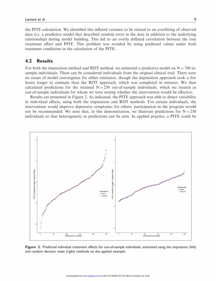
For both the imputation method and RDT method, we estimated a predictive model on N¼ 760 in-sample individuals. These can be considered individuals from the original clinical trial. There wereno issues of model convergence for either estimator, though the imputation approach took a fewhours longer to estimate than the RDT approach, which was completed in minutes. We thencalculated predictions for the retained N¼ 250 out-of-sample individuals, which we treated asout-of-sample individuals for whom we were testing whether the intervention would be effective.

Results are presented in Figure 2. As indicated, the PITE approach was able to detect variabilityin individual effects, using both the imputation and RDT methods. For certain individuals, theintervention would improve depressive symptoms; for others, participation in the program wouldnot be recommended. We note that, in this demonstration, we illustrate predictions for N¼ 250individuals so that heterogeneity in predictions can be seen. In applied practice, a PITE could be

Figure 2. Predicted individual treatment effects for out-of-sample individuals, estimated using the imputation (left)

and random decision trees (right) methods on the applied example.

Lamont et al. 9



estimated for a single individual. The strength and direction of the prediction could then be usedduring treatment planning for that individual.

Comparing across predictive methods, RDT approach tended to produce estimates closer to themean, whereas the imputation approach provided a wider range of PITE values. The simulationstudy in the next section is intended to test which is providing more accurate and stable predictions.

5 Simulation study

One of the limitations of the applied example is that we do not know the true effects of theindividuals in the sample, making the accuracy of the estimates unknown. In this section, wepresent the results of a Monte Carlo simulation study used to test the quality of these estimatedindividual effects.

5.1 Methods

Data were generated in R software version 3.1.3.66 A total of N¼ 10,000 independent and identicallydistributed cases were generated. Fifty percent of the cases (N¼ 5000) were used for the derivationof predictive models, and the remaining N¼ 5000 cases were reserved for out-of-sample estimation.Cases were randomly assigned to balanced treatment and control groups.

Following the design of the BSF trial, data were generated with the same number of categoricalcovariates as the applied data. The true value under control was generated as Yc � Nð0, 1Þ. The truetreatment effect for each individual was linearly related to a set of seven binary baseline covariates,generated using the following equation

TE ¼ �1:3 X1ð Þ � 1:2 X2ð Þ � :6 X3ð Þ þ :3 X4ð Þ þ :5 X5ð Þ þ 1:1 X6ð Þ þ 1:2 X7ð Þ:

Binary covariates (generated from a random binomial distribution with the probability ofendorsement equal to .5) were used to resemble the design of the data in the motivating example,which included only categorical predictors. No modifications would be necessary to extend tocontinuous predictors. Effect sizes were selected so that the mean effect was near zero (but notcompletely symmetric around zero) with individual effect ranging from small to large. Since thePITE approach is designed to detect HTE without pre-specifying the variable(s) responsible for thedifferential effects, we wanted to include a comprehensive set of potential confounders, most ofwhich end up being nuisance variables. Thus, we additionally included 68 nuisance variables whosecoefficients (X8 through X75) were set to zero. The true response under treatment (Yt) was defined asYti ¼ Yci þ TE for that individual.

One hundred repetitions of the simulated data were generated. Baseline covariates (and byextension the true treatment effects) were set to be the same across repetitions. This established ascenario where the same individual was repeated, allowing for intuitive interpretations about thenumber of times an individual’s predicted value reflects the true treatment effect. Yc (and byextension Yt) varied across repetitions. The procedures for estimating the predictive models andfor calculating PITEs in this simulation study were identical to those used in the applied example(above).

We note that since this is our first study on the PITE approach, we specifically designed theseconditions to be optimal in the sense of a correctly specified model with no major violations ofmodel assumptions (e.g. all effect moderators observed and exchangeability of the in-sample andout-of-sample individuals) and a large sample size. While this may limit generalizability to other




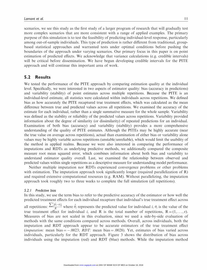
scenarios, we see this study as the first study of a larger program of research that will gradually testmore complex scenarios that are more consistent with a range of applied examples. The primarypurpose of this simulation is to test the feasibility of predicting individual-level response, particularlyamong out-of-sample individuals. This type of prediction is rather different from traditional, group-based statistical approaches and warranted tests under optimal conditions before pushing theboundaries of the approach under varying scenarios. Our primary focus in this paper is on pointestimation of predicted effects. We acknowledge that variance calculations (e.g. credible intervals)will be critical before dissemination. We have begun developing credible intervals for the PITEapproach and will continue this important area of work.

5.2 Results

We tested the performance of the PITE approach by comparing estimation quality at the individuallevel. Specifically, we were interested in two aspects of estimator quality: bias (accuracy in predictions)and variability (stability) of point estimates across multiple repetitions. Because the PITE is anindividual-level estimate, all statistics were calculated within individuals across repetitions. We definedbias as how accurately the PITE recaptured true treatment effects, which was calculated as the meandifference between true and predicted values across all repetitions. We examined the accuracy of theestimate for each individual, rather than a single summative measure for the whole sample. Variabilitywas defined as the stability or reliability of the predicted values across repetitions. Variability providedinformation about the degree of similarity (or dissimilarity) of repeated predictions for an individual.Examination of both bias (accuracy) and variability (stability) provides a more comprehensiveunderstanding of the quality of PITE estimates. Although the PITEs may be highly accurate (nearthe true value on average across repetitions), actual than examination of either bias or variability alonevalues may be highly variable across repetitions (unstable/unreliable), which would limit the usability ofthe method in applied realms. Because we were also interested in comparing the performance ofimputations and RDTs as underlying predictive methods, we additionally compared the compositemeasure root mean squared error, which combines information about both bias and variability tounderstand estimator quality overall. Last, we examined the relationship between observed andpredicted values within single repetitions as a descriptive measure for understanding model performance.

Neither multiple imputation nor RDTs experienced convergence problems or other problemswith estimation. The imputation approach took significantly longer (required parallelization of R)and required extensive computational resources (e.g. RAM). Without parallelizing, the imputationapproach took roughly two to three weeks to complete the full simulation (all repetitions).

5.2.1 Predictive bias

In this study, we use the term bias to refer to the predictive accuracy of the estimator or how well thepredicted treatment effects for each individual recapture that individual’s true treatment effect across

all repetitions:

Pr

1½�i��i�iR where �i represents the predicted value for individual i, �i is the value of the

true treatment effect for individual i, and R is the total number of repetitions, R¼ (1, . . . , r).Measures of bias are not scaled in this evaluation, since we used a side-by-side evaluation ofmethods with the same conditions compared across methods. Overall, across individuals, both theimputation and RDT approach appear to be accurate estimators of the true treatment effect(imputation: mean bias¼�.0023; RDT: mean bias¼ .0028). Yet, estimates of bias varied acrossindividuals, particularly for the RDT approach. Figure 3 shows the distribution of bias acrossindividuals using the imputation (red) and RDT (blue) methods. While the imputation method

Lamont et al. 11



produced fairly unbiased estimates for all individuals, the RDT method showed substantial bias forsome individuals. In fact, despite being unbiased at the mean, the range of estimated bias acrossindividuals ranged from �0.8711 to 0.8536 using the RDT method (compared to �0.0688-0.0600using the imputation method).

To further explore for whom the RDT method may be producing biased results, we examinedbias as a function of the true treatment effect. As seen in Figure 4, there is minimal relation betweenbias and a true treatment effect for the imputation method but a fairly strong relation between anindividual’s true treatment effect and bias for the RDT method. The RDT method performs well forindividuals in the mid-range, but does not provide accurate estimates of treatment effects forindividuals at the extremes.

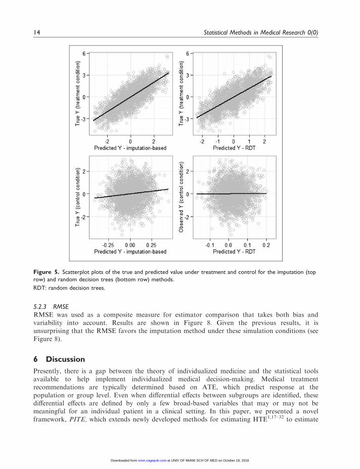
We then investigated, within one randomly selected repetition, the relationship between the trueY under treatment and control and the predicted Y for the same condition. This was intended todiagnose potential pitfalls in the estimation. Results are presented in Figure 5. The top row showsthe scatterplot for the imputation method, the bottom row uses the RDT method. Using bothestimators, the PITE approach performed as expected. There was no relationship betweenpredicted values and true values under control (which is consistent with the data generation) anda moderate relationship under treatment. Figure 6 shows the plots of true versus predicted treatmenteffect (Yt�Yc) using the imputation method (left) and RDT (right), with colors representing thetreatment condition to which the individual was randomized. Consistent with previous results, theimputation method produced estimates that were highly related to true values without any apparentbias in the parameter space. The RDT method produced estimates with more error in the prediction,particularly at the tails of the distribution. Extreme true values tended to be downward biased.

Figure 3. Distribution of individual-level bias using the imputation (red) and random decision trees (blue)

estimators.




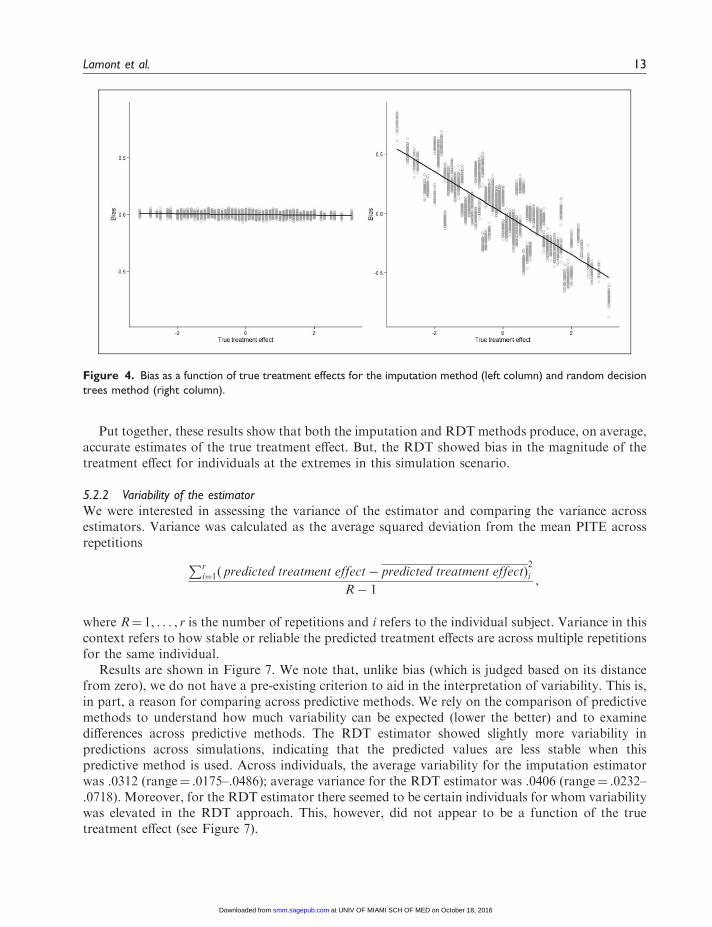
Put together, these results show that both the imputation and RDT methods produce, on average,accurate estimates of the true treatment effect. But, the RDT showed bias in the magnitude of thetreatment effect for individuals at the extremes in this simulation scenario.

5.2.2 Variability of the estimator

We were interested in assessing the variance of the estimator and comparing the variance acrossestimators. Variance was calculated as the average squared deviation from the mean PITE acrossrepetitions

Pri¼1ð predicted treatment effect� predicted treatment effectÞ

2

i

R� 1,

where R¼ 1, . . . , r is the number of repetitions and i refers to the individual subject. Variance in thiscontext refers to how stable or reliable the predicted treatment effects are across multiple repetitionsfor the same individual.

Results are shown in Figure 7. We note that, unlike bias (which is judged based on its distancefrom zero), we do not have a pre-existing criterion to aid in the interpretation of variability. This is,in part, a reason for comparing across predictive methods. We rely on the comparison of predictivemethods to understand how much variability can be expected (lower the better) and to examinedifferences across predictive methods. The RDT estimator showed slightly more variability inpredictions across simulations, indicating that the predicted values are less stable when thispredictive method is used. Across individuals, the average variability for the imputation estimatorwas .0312 (range¼ .0175–.0486); average variance for the RDT estimator was .0406 (range¼ .0232–.0718). Moreover, for the RDT estimator there seemed to be certain individuals for whom variabilitywas elevated in the RDT approach. This, however, did not appear to be a function of the truetreatment effect (see Figure 7).

Figure 4. Bias as a function of true treatment effects for the imputation method (left column) and random decision

trees method (right column).

Lamont et al. 13



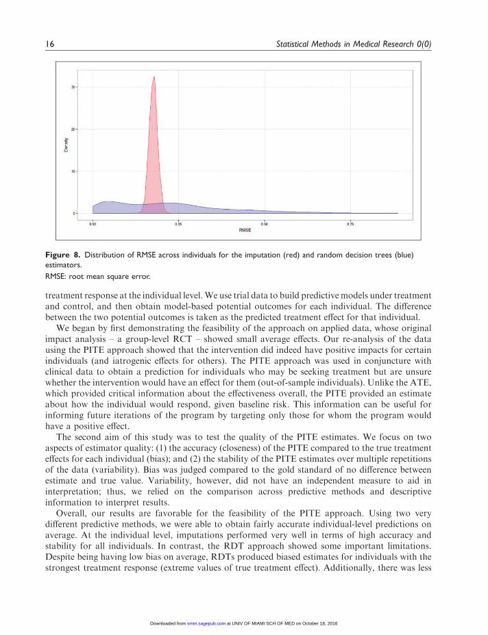
5.2.3 RMSE

RMSE was used as a composite measure for estimator comparison that takes both bias andvariability into account. Results are shown in Figure 8. Given the previous results, it isunsurprising that the RMSE favors the imputation method under these simulation conditions (seeFigure 8).

6 Discussion

Presently, there is a gap between the theory of individualized medicine and the statistical toolsavailable to help implement individualized medical decision-making. Medical treatmentrecommendations are typically determined based on ATE, which predict response at thepopulation or group level. Even when differential effects between subgroups are identified, thesedifferential effects are defined by only a few broad-based variables that may or may not bemeaningful for an individual patient in a clinical setting. In this paper, we presented a novelframework, PITE, which extends newly developed methods for estimating HTE1,17–32 to estimate

Figure 5. Scatterplot plots of the true and predicted value under treatment and control for the imputation (top

row) and random decision trees (bottom row) methods.

RDT: random decision trees.




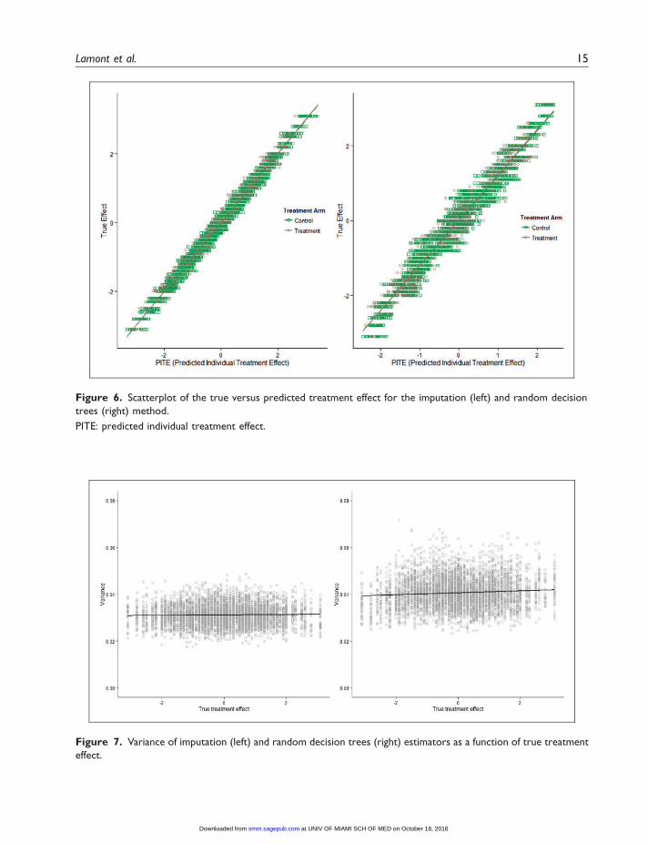
Figure 7. Variance of imputation (left) and random decision trees (right) estimators as a function of true treatment

effect.

Figure 6. Scatterplot of the true versus predicted treatment effect for the imputation (left) and random decision

trees (right) method.

PITE: predicted individual treatment effect.

Lamont et al. 15



treatment response at the individual level.We use trial data to build predictivemodels under treatmentand control, and then obtain model-based potential outcomes for each individual. The differencebetween the two potential outcomes is taken as the predicted treatment effect for that individual.

We began by first demonstrating the feasibility of the approach on applied data, whose originalimpact analysis – a group-level RCT – showed small average effects. Our re-analysis of the datausing the PITE approach showed that the intervention did indeed have positive impacts for certainindividuals (and iatrogenic effects for others). The PITE approach was used in conjuncture withclinical data to obtain a prediction for individuals who may be seeking treatment but are unsurewhether the intervention would have an effect for them (out-of-sample individuals). Unlike the ATE,which provided critical information about the effectiveness overall, the PITE provided an estimateabout how the individual would respond, given baseline risk. This information can be useful forinforming future iterations of the program by targeting only those for whom the program wouldhave a positive effect.

The second aim of this study was to test the quality of the PITE estimates. We focus on twoaspects of estimator quality: (1) the accuracy (closeness) of the PITE compared to the true treatmenteffects for each individual (bias); and (2) the stability of the PITE estimates over multiple repetitionsof the data (variability). Bias was judged compared to the gold standard of no difference betweenestimate and true value. Variability, however, did not have an independent measure to aid ininterpretation; thus, we relied on the comparison across predictive methods and descriptiveinformation to interpret results.

Overall, our results are favorable for the feasibility of the PITE approach. Using two verydifferent predictive methods, we were able to obtain fairly accurate individual-level predictions onaverage. At the individual level, imputations performed very well in terms of high accuracy andstability for all individuals. In contrast, the RDT approach showed some important limitations.Despite being having low bias on average, RDTs produced biased estimates for individuals with thestrongest treatment response (extreme values of true treatment effect). Additionally, there was less

Figure 8. Distribution of RMSE across individuals for the imputation (red) and random decision trees (blue)

estimators.

RMSE: root mean square error.




stability in PITE estimates using the RDT approach than the imputation approach, at least inscenarios that match our data-generation model. Put together, these findings suggest that theRDT approach may not be a suitable estimator of PITE, despite having favorable properties foruncovering HTE in general.55,68

We expect that many established methods for estimating HTE can be used to derive predictions.We focused on two rather distinct methods in this study; and, despite the outperformance of theimputation method in our analysis, we emphasize that there is likely no single optimal predictivemethod.55 The scenario we designed in this simulation was correctly specified for the imputationmethod (e.g. involved all the right covariates and interaction); therefore, it was not surprising thatthe imputations worked very well. A similar finding is reported by Hastieet al.,69 where a linearmodel is shown to perform better than RDT in a scenario where the true model is linear. Thecorrectly specified design was intentional, as the purpose was, in some sense, proof of conceptthat using methods designed for HTE can be used for individual predictions.

Future work is planned that will explore the limits of the methods under conditions of increasedcomplexity. We anticipate that, for example, as higher order interactions are introduced to the data,the RDT method (along with other tree-based methods) will outperform the imputation approach.This expectation is based on the way that imputations and RDTs handle interactive effects. WhereasRDTs can easily accommodate interactions without any additional model specifications,imputations require the interactions to be specified in the imputation model. This creates ascenario in which the analyst must have a priori theory about which higher order interactions aredriving heterogeneity in effects (which is arguably an unlikely situation), and a sufficient sample sizeto estimate a rather large and complex imputation equation. It is likely that inclusion of multiplehigher order interaction to an already large imputation model will cause estimation problems and/orencounter problems of statistical power. In addition, another important area of future work forexpanding the PITE framework is the handling of missingness of observed data. In this study, weused single imputation of covariates and full information maximum likelihood (FIML) on outcomesin the applied study. The implications of this approach need to be more fully explored. A likelylimitation of the PITE method is the case of differential attrition, particularly when imbalanceddrop-out is informative. While missingness on the outcome is itself non-problematic, we suspect thatinformative differential attrition will lead to bias on the estimate of the response on treatment and,consequently, the PITE, unless the mechanism driving the differential attrition of modeled.

We acknowledge that the fundamental purpose of the potential outcomes framework is to comeup with causal estimates at the population level. In this study, we presented an extension of thepotential outcomes framework where we derived model-based estimates of potential outcomes underboth treatment and control. Since the models tested in this study were correctly specified, additionalwork is needed to understand the assumptions required for these model-based individual estimates(rather than population estimates) as pure, causal effects. Related, this study presents a computer-assisted simulation as a conjecture of the PITE framework. We do not see this as a completereplacement for a formal mathematical proof; however, given our purposes of understanding themethod and the conditions under which the method works, we see this approach as well fitting.

The PITE approach marks a first step to integrating a diverse methodological literature on HTEand provides a framework for increasing the clinical utility of established methods. The PITEapproach directly focuses on the estimation of predicted effects for individuals who were not partof the original clinical trial. While extrapolation to external data is possible with many tree-basedand regression-based models, this practice is often not empirically tested for accuracy and thereforerarely advised. In this study, we explicitly focus on out-of-sample predictions. This is an importantaspect of this work because it – along with the focus on individual-level estimation – holds the

Lamont et al. 17



potential to transform the ways in which treatment decisions in the practice of behavioral and healthmedicine are made. This type of prediction can greatly advance individualized medicine by providinginterventionists and patients access to important individual-level data during treatment selection,prior to the initiation of a treatment protocol. The customization of treatment to the individual canpotentially enhance the quality and cost-efficiency of services by allocating treatments to only thosewho are most likely to benefit.

Declaration of conflicting interests

The author(s) declared no potential conflicts of interest with respect to the research, authorship, and/or

publication of this article.

Funding

The author(s) disclosed receipt of the following financial support for the research, authorship, and/or

publication of this article: This work was supported by grant MR/L010658/1 from the Medical Research

Council of the United Kingdom, awarded to Principal Investigator, Thomas Jaki, PhD.

References

1. Huang Y, Gilbert PB and Janes H. Assessing treatment-selection markers using a potential outcomes framework.Biometrics 2012; 68: 687–696.

2. Li A and Meyre D. Jumping on the train of personalizedmedicine: a primer for non-geneticist clinicians: part 3.Clinical applications in the personalized medicine area.Curr Psychiatry Rev 2014; 10: 118–132.

3. Goldhirsch A, Winer EP, Coates AS, et al. Personalizingthe treatment of women with early breast cancer:highlights of the St Gallen International expert consensuson the primary therapy of early breast cancer 2013. AnnOncol 2013; 24: 2206–2223.

4. Aquilante CL, Langaee TY, Lopez LM, et al. Influence ofcoagulation factor, vitamin K epoxide reductase complexsubunit 1, and cytochrome P450 2C9 gene polymorphismson warfarin dose requirements. Clin Pharmacol Ther 2006;79: 291–302.

5. Assmann SF, Pocock SJ and Enos LE. Subgroup analysisand other (mis)uses of baseline data in clinical trials.Lancet 2000; 355: 1064–1069.

6. Pocock SJ, Assmann SE, Enos LE, et al. Subgroupanalysis, covariate adjustment and baseline comparisons inclinical trial reporting: current practice and problems. StatMed 2002; 21: 2917–2930.

7. Brookes ST, Whitley E, Peters TJ, et al. Subgroup analysesin randomised controlled trials: quantifying the risks offalse-positives and false-negatives. Health Technol Assess2001; 5: 1–56.

8. Cui L, James Hung HM, Wang SJ, et al. Issues related tosubgroup analysis in clinical trials. J Biopharm Stat 2002;12: 347.

9. Fink G, McConnell M and Vollmer S. Testing forheterogeneous treatment effects in experimental data: falsediscovery risks and correction procedures. J Dev Eff 2014;6: 44–57.

10. Lagakos SW. The challenge of subgroup analyses –reporting without distorting. N Engl J Med 2006; 354:1667–1669.

11. Wang R, Lagakos SW and Ware JH. Statistics in medicine– reporting of subgroup analyses in clinical trials. N Engl JMed 2007; 357: 2189–2194.

12. Neyman J. Sur les applications de la theorie desprobabilites aux experiences agricoles: essai des principes(Masters Thesis); Justification of applications of thecalculus of probabilities to the solutions of certainquestions in agricultural experimentation. ExcerptsEnglish translation (Reprinted). Stat Sci 1923; 5:463–472.

13. Rubin DB. Estimating causal effects of treatments inrandomized and nonrandomized studies. J Educ Psychol1974; 66: 688–701.

14. Rubin DB. Formal modes of statistical inference for causaleffects. J Stat Plan Inference 1990; 25: 279–292.

15. Rubin DB. Causal inference using potential outcomes.J Am Stat Assoc 2005; 100: 322–331.

16. Holland PW. Statistics and causal inference. J Am StatAssoc 1986; 81: 945–960.

17. Basu A. Estimating person-centered treatment (PeT)effects using instrumental variables: an application toevaluating prostate cancer treatments. J Appl Econ 2014;29: 671–691.

18. Foster JC, Taylor JM and Ruberg SJ. Subgroupidentification from randomized clinical trial data. StatMed 2011; 30: 2867–2880.

19. Doove LL, Dusseldorp E, Deun K, et al. A comparison offive recursive partitioning methods to find personsubgroups involved in meaningful treatment–subgroupinteractions. Adv Data Anal Classif 2013; 1–23.

20. Freidlin B, McShane LM, Polley MY, et al. Randomizedphase II trial designs with biomarkers. J Clin Oncol 2012;30: 3304–3309.

21. Imai K and Ratkovic M. Estimating treatment effectheterogeneity in randomized program evaluation. AnnAppl Stat 2013; 7: 443–470.

22. Imai K and Strauss A. Estimation of heterogeneoustreatment effects fromrandomized experiments, withapplication to the optimal planning of the Get-Out-the-Vote campaign. Polit Anal 2011; 19: 1–19.

23. Heckman JJ, Urzua S and Vytlacil E. Understandinginstrumental variables in models with essentialheterogenetiy. Rev Econ Stat 2006; 88: 389–432.




24. Zhang Z, Wang C, Nie L, et al. Assessing the heterogeneityof treatment effects via potential outcomes of individualpatients. J R Stati Soc C 2013; 62: 687–704.

25. Bitler MP, Gelbach JB and Hoynes HW. Can variation insubgroups’ average treatment effects explain treatmenteffect heterogeneity? Evidence from a social experiment,National Bureau of Economic Research, NBER WorkingPaper No. 20142, May 2014. Available at: http://www.nber.org/papers/w20142.

26. Green DP and Kern HL. Modeling heterogeneoustreatment effects in survey experiments with Bayesianadditive regression trees. Public Opin Quart 2012; 76:491–511.

27. Shen C, Jeong J, Li X, et al. Treatment benefit andtreatment harm rate to characterize heterogeneity intreatment effect. Biometrics 2013; 69: 724–731.

28. Simon N and Simon R. Adaptive enrichment designs forclinical trials. Biostatistics 2013; 14: 613–625.

29. Rosenbaum PR. Confidence intervals for uncommon butdramatic responses to treatment. Biometrics 2007; 63:1164–1171.

30. Poulson RS, Gadbury GL and Allison DB. Treatmentheterogeneity and individual qualitative interaction. AmStat 2012; 66: 16–24.

31. Cai T, Tian L, Wong PH, et al. Analysis of randomizedcomparative clinical trial data for personalized treatmentselections. Biostatistics 2011; 12: 270–282.

32. Ruberg SJ, Chen L and Wang Y. The mean does not meanas much anymore: finding sub-groups for tailoredtherapeutics. Clin Trials 2010; 7: 574–583.

33. Gadbury G, Iyer H and Allison D. Evaluating subject-treatment interaction when comparing two treatments.J Biopharm Stat 2001; 11: 313.

34. Gadbury GL and Iyer HK. Unit-treatment interaction andits practical consequences. Biometrics 2000; 56: 882–885.

35. Gadbury GL, Iyer HK and Albert JM. Individualtreatment effects in randomized trials with binaryoutcomes. J Stat Plan Inference 2004; 121: 163.

36. Nomi T and Raudenbush SW. Understanding treatmenteffects heterogeneities using multi-site regressiondiscontinuity designs: example from a ‘‘Double-Dose’’Algebra Study in Chicago. Chicago: Society for Researchon Educational Effectiveness, 2012.

37. Na C, Loughran TA and Paternoster R. On theimportance of treatment effect heterogeneity inexperimentally-evaluated criminal justice interventions.J Quant Criminol 2015; 31: 289–310.

38. Schapire RE and Freund Y. Boosting: foundations andalgorithms. Cambridge, MA: MIT Press, 2012.

39. LeBlanc M and Kooperberg C. Boosting predictions oftreatment success. Commentary 2010; 107: 13559–13560.

40. Lipkovich I and Dmitrienko A. Strategies for identifyingpredictive biomarkers and subgroups with enhancedtreatment effect in clinical trials using SIDES. J BiopharmStat 2014; 24: 130–153.

41. Zhang Z, Qu Y, Zhang B, et al. Use of auxiliary covariatesin estimating a biomarker-adjusted treatment effect modelwith clinical trial data. Stat Meth Med Res. Epub ahead ofprint 16 December 2013. DOI: 10.1177/0962280213515572.

42. Su X and Johnson WO. Interaction trees: exploring thedifferential effects of intervention programme for breastcancer survivors. J R Stat Soc C 2011; 60: 457–474.

43. Su X, Kang J, Fan J, et al. Facilitating score and causalinference trees for large observational studies. J MachLearn Res 2012; 13: 2955–2994.

44. Kang J, Su X, Hitsman B, Liu K, et al. Tree-structuredanalysis of treatment effects with large observational data.J Appl Stat 2012; 39: 513–529.

45. Lipkovich I, Dmitrienko A, Denne J, et al. Subgroupidentification based on differential effect search – a recursive

partitioning method for establishing response to treatmentin patient subpopulations. Stat Med 2011; 30: 2601–2621.

46. Su X, Tsai C-L, Wang H, et al. Subgroup analysis viarecursive partitioning. JMach Learn Res 2009; 10: 141–158.

47. Su X, Zhou T, Yan X, et al. Interaction trees with censoredsurvival data. Int J Biostat 2008; 4: 1–26.

48. Zeileis ATK. Model-based recursive partitioning.J Comput Graph Stat 2008; 17: 492–514.

49. Dusseldorp E, ConversanoC andVanOsBJ. Combining anadditive and tree-based regression model simultaneously:STIMA. J Comput Graph Stat 2010; 19: 514–530.

50. Ciampi A, Negassa A and Lou Z. Tree-structuredprediction for censored survival data and the Cox model.J Clin Epidemiol 1995; 48: 675–689.

51. Dai JY, Kooperberg C, Leblanc M, et al. Two-stagetesting procedures with independent filtering for genome-wide gene-environment interaction. Biometrika 2012; 99:929–944.

52. Dixon DO and Simon R. Bayesian subset analysis.Biometrics 1991; 47: 871–881.

53. Gail M and Simon R. Testing for qualitative interactionsbetween treatment effects and patient subsets (withappendix). Biometrics 1985; 41: 361–372.

54. Simon R. Bayesian subset analysis: application to studyingtreatment-by-gender interactions. Stat Med 2002; 21:2909–2916.

55. Malley JD, Malley KG and Pajevic S. Statistical learningfor biomedical data. New York: Cambridge UniversityPress, 2011.

56. Schafer JL. Analysis of incomplete multivariate data. NewYork: Chapman & Hall/CRC, 1997.

57. Little RJA and Rubin DB. Statistical analysis with missingdata, 2nd ed. New York: John Wiley, 2002.

58. Rubin DB. Multiple imputation for nonresponse in surveys.New York: J Wiley & Sons, 1987.

59. Dore DD, Swaminathan S, Gutman R, et al. Differentanalyses estimate different parameters of the effect oferythropoietin stimulating agents on survival in end stagerenal disease: a comparison of payment policy analysis,instrumental variables, and multiple imputation of potentialoutcomes. J Clin Epidemiol 2013; 66(8 Suppl): S42–S50.

60. Raghunathan TE, Lepkowski JM, Van Hoewyk J, et al.A multivariate technique for multiply imputing missingvalues using a sequence of regression models. SurvMethodol 2001; 27: 85–95.

61. Hershey A, Devaney B, Wood RG, et al. Building StrongFamilies (BSF) project data collection, 2005–2008. AnnArbor, MI: Inter-university Consortium for Political andSocial Research [distributor], 2011.

62. Inter-university Consortium for Political and SocialResearch, www.icpsr.umich.edu/icpsrweb/ICPSR/studies/29781 (accessed 5 December 2015).

63. Radloff LS and Radloff LS. Center for EpidemiologicStudies Depression Scale. The CES-D Scale: a self-reportdepression scale for research in the general population.Appl Psychol Meas 1977; 1: 385–401.

64. Muthen LK and Muthen BO. Mplus user’s guide, 7th ed.Los Angeles: Muthen & Muthen, 1998–2012.

65. Su Y-S, Gelman A, Hill J and Masanao Y. Multipleimputation with diagnostics (mi) in R: opening windowsinto the black box. J Stat Software 2011; 45: 1–31.

66. R Core Team. R: a language and environment for statisticalcomputing. Vienna, Austria: R Foundation for StatisticalComputing, 2015.

67. Liaw A and Wiener M. Classification and regression byrandom forest. R News 2002; 2: 18–22.

68. Breiman L. Random forests. Mach Learn 2001; 45: 5–32.69. Hastie T, Tibshirani R and Friedman J. The elements of

statistical learning: data mining, inference, and prediction,2nd ed. New York: Springer, 2009, p.xxii.

Lamont et al. 19


http://www.nber.org/papers/w20142

http://www.nber.org/papers/w20142

www.icpsr.umich.edu/icpsrweb/ICPSR/studies/29781

www.icpsr.umich.edu/icpsrweb/ICPSR/studies/29781


Documents

Identification of predicted individual treatment effects ...hishwaran/papers/SMMR.2016.pdf · individual treatment effects in randomized clinical trials ... Even in the case of cutting-edge,