Embed Size (px)
Citation preview
L ID-A134 731 CHEMICAL CLR1FICRTION METHODS FOR CONFINED DREDGED 1/~MATERIAL DISPOSAL(U) ARMY ENGINEER NATERbIRYS EXPERIMENTI STATION VICKSBURG MS P R SCHROEDER JUL 83
EUEEEEhEhEEEEEEENCREhhES-hEEE32 F 3/ENmhhE7hhEEEhhmhohmhhhEEEEohEEEmhmhEEEI
11111 I12.0
IIR-
12 1.A11111__..6: L
MICROCOPY RESOLUTION TEST CHART
NATiONAL BUREAU OF STONDARDS 1963-
F--
FOX
DREDGING OPERATIONSTECHNICAL SUPPORT
TECHNICAL REPORT D-83-2
CHEMICAL CLARIFICATIONMETHODS FOR CONFINED DREDGED
MATERIAL DISPOSAL
by
Paul R. Schroeder
Environmental LaboratoryU. S. Army Engineer Waterways Experiment Station
P. 0. Box 631, Vicksburg, Miss. 39180
July 1983Final Report
Approved For Public Release. Distribution Unlimited
A
DTI~E -CTE
'Ilk
111100111111Proparp1 f- Office, Chief of Engineers, U S ArmyWashington.~C, 203 14
E:f3
-5 J
Destroy this report when no longer needed. Do not returnit to the originator.
The findings in this report are not to be construed as an officialDepartment of the Army position unless so designated
by other authorized documents.
The contents of this report are not to be used foradvertising, publication, or promotional purposes.Citation of trade names does not constitute anofficial endorsement or approval of the use of
such commercial products.
This report series includes publications of thefollowing programs:
Dredging Operations Technical Support~DOTS)
Long-Tcrm Effects of Dredging Operations(LEDO)
Interagency Field Verification of Methodologies forEvaluating Dredged Material Disposal Alternatives
(FVP)
*1
[IL i ash t Iil4 SECURITY CLASSIFICAT;ON OF THIS PAGE ""oen Dwe Entered)
'4 ~READ 11NSTRLTCTIONSREPORT DOCUMENTATION PAGE BEFORE COMPLETING FORM1. REPORT NUMBER 2.GOVT ACCESSION No. 3. qECIPIENT'S CATALOG NUMBER
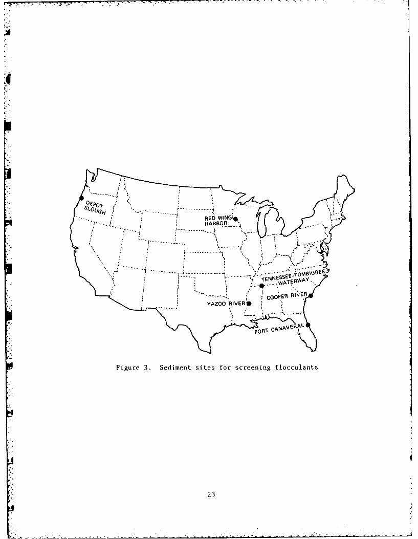
Fechni icai Report J)-
4. TITLE (and Subtitle) S TYPE OF REPORT & PERIO COVERED
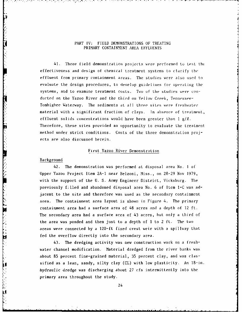
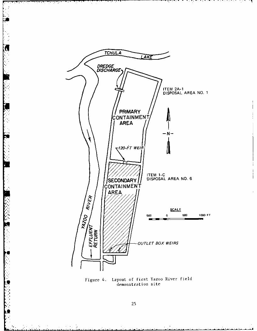
CIIEN CAL CLAR I FICAT 1-IN 9EITOI)S HI' 0IR NE I NK) iiRlI~ioE inal reort'lATER [AL DISPoSAL
7. AUTHOR(&) S OTATO RN UBR&
L9. PERFORMING ORGANIZATION NAME AND ADDRESS 10. PROGRAM ELEMENT PROJECT, TASKL AREA & WORK UNIT NUMBERS
U. S. Armyv Enigineer lolterwuys F~Xperiment Stat iolEnvi ronmentalI Laboraitorv D~reing OpeiO1ti oIlsP. o1. Box, bi VikksbiirK 'liss. )180 10) l~ll il Support Prig .111
It. CONTROLLING OFFICE N AME AND ADDRESS 12. REPORT DATE
Off ice, Chief of Engineers, U. S. Army IIIv 1961Wiashington, D. C. 20Hf4 13. NUMBER OF PAGES
14714. MONITORING AGENCY NAME &ADDRESS(if different froml Conitrolling Office) 15. SECURITY CLASS. (of this report)
Unclassiflied
15.. DECL ASSIFICATION/ DOWNGRADINGSCHEDULE
16. DISTRIBUTION STATEMENT (of this Report)
Approvedl for publico release; distribution unlimited.
17. DISTRIBUTION STATEMENT (of the abstract entered In Block 20, If different from Report)
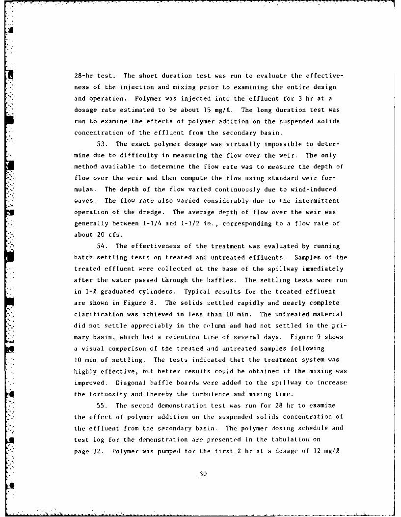
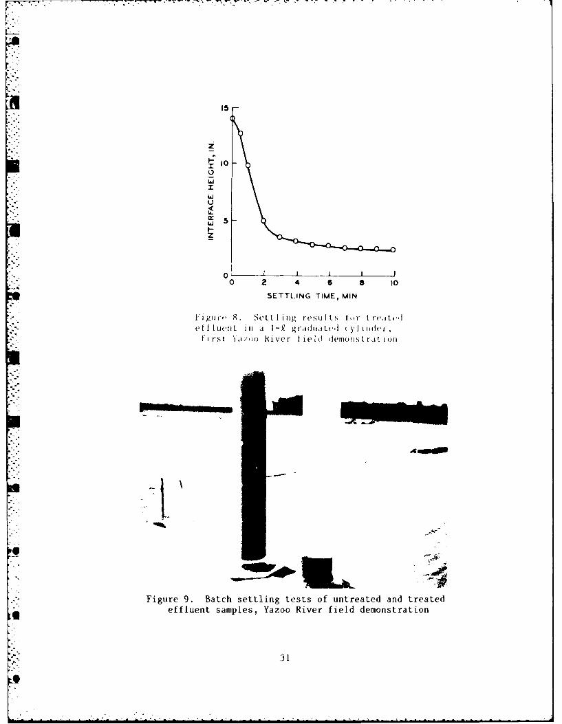
IS. SUPPLEMENTARY NOTES
Avail[able from National Technical Infoirmlationl Servih, 5285~ Port Royal Road. Sprin~gfield, Va. 22161.
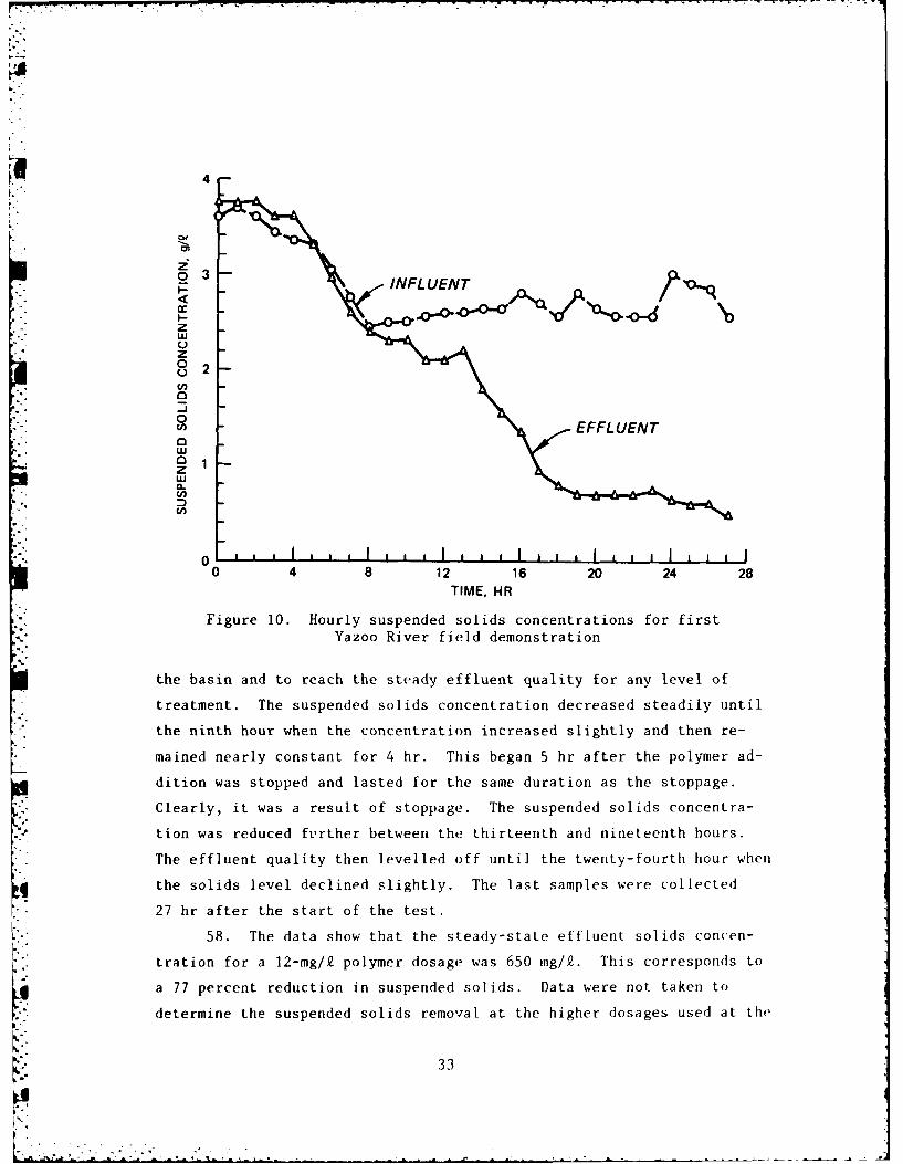
It. KEY WORDS (Continue an reverse side It necessary and Identify by block numrber)
[jred.'od r. ,ri il di i sal
io 1% I.
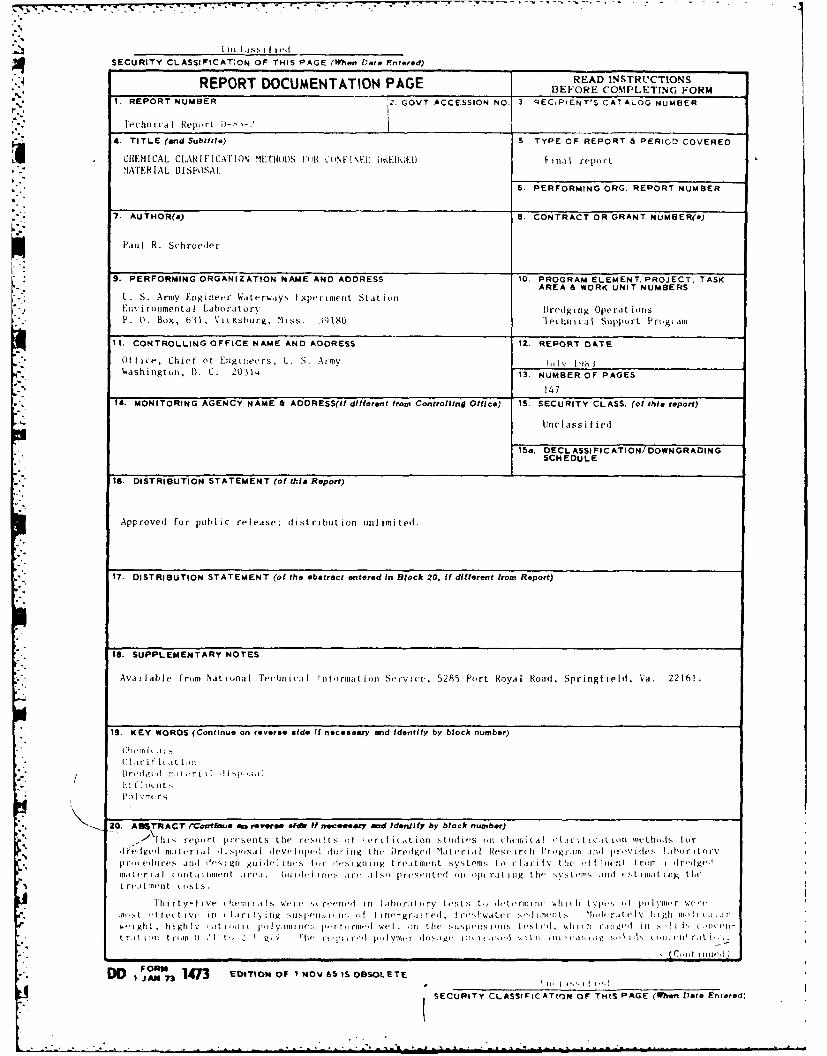
20. AST"ACT rCcztu* rnePoerse* eif I neceeau ad Idenjify, by block numtber)
hI reoirt 1) esetiLs t he r si ItL..- I cr i f i (.,Lion stiiilioes ont )hcioha i I c,, i I k L oluL nhi.,Is orIrlil ri Iter,,~ Isisl I ileve Iop d~e lii, r hg I hi Dredgeid '1a tioria I lls~rc, Priigi'llii and 1 proi des I ahoiir.i torvp)ri i t ires and! de,,s, gri gio I', I Itic's lIi o I d's I gn iy Ig ri'.,ini'rit systLems, to (la ti Iv It( li I ! iorit I rim j d lreI' i.
t roilill t ist 5.
Thi rty-fivye firiii ials ttii' si reiii' in lal'or,itiirv lists Ii, deteininlit, 0 1h tpI',s i. I i \iirmist IIfc t ivv iii 1jrin ig swii5 1 iH.i.,if I iroi-gr.inreil. ,i'~~t' s'lmn-iI. i i~ilj ligh, 115,k1 l
IgIut . hI glu it-, , in 111 1 1i jii l u iirw:-. I-i tr I , woE1 t I I ol lit, sutispenI ,its i s I rdAiIi. s k h, r~igvdi 111 -i ,I I' k t ell-r lit u 1.11r Iull '. 0 i h" , Itro ilki i Id " 1 Viw I, i l gH HI iti.1 "1s ' 11 S iu flu '"i1rl iz s,1 iifl. l 1 .rtuuI,.
WO JAN73 147n EltTIOWOF I MOV 65S OBSOLETE . .
SECURITY CLASSIFICATION OF THIS PAGE (When Vets Entered)
* SECURITY CLASSIFICATION OF THIS PAGE(Whmai Data Rnte.ed)
20. ABSTRACT (Colltinued)
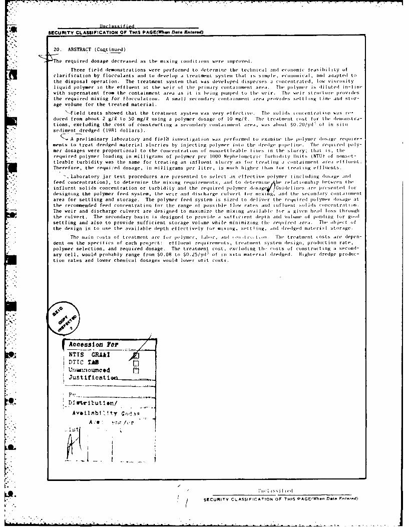
The required dosage decreased as the mixing conidi tions were improved.
Three field demonstrat ions were performred to dleterine tihe techical Can ut'oromil ( easib ili ty ofclarification by flocculants and to dievelop a treatmient system that is simple. economical , arid dapted tothe disposal operation. The treatmeint system that was developed disperses a concentrated, low viscosity
* ~~liquid polymer in the effluent at the weir of thre primiary conrtainmlerit area. The polyirrer is di liitr't in-i ii
with supernatant from the conta inmerit area as it is bieinrg puimped to the we ir. Thre we ir st rictrrr prttvrdr's* ~~the required mix inrg for fl1occulIat ioin. A siiall seciirda ry corit aiinment a rea proides set tlinrg t imte anrd sitor-* age volume for the treated material.
'--Field tests showed that the treatment systenm was very effective. the solidis coiicrnt rat i ito was re-duced from about 2 g/2 to 50 mg/I using a p~olyme'r dosage of 10 rig/I. The t reatmenrt lo~st for the demionist ra-tions, excluding the cost of constructing a secondary corita inint a rea, was about SO. 20/yd' of iii sitnisediment dredged (1981 dollars).
(-A preliminary labora tory arid fie]ld ives t igat iot) wars per formedi to exainie t he po Iyrir'r dosige requri re-ments to treat dredged material sluirr ies by i nj ect inrg polymner init o the dred ge iptirIine. Thie reqiired ptoly-mer dosages were proportional to the concentration of rrorsett leablr' f ines ti the slurry; tha~t is, therequired polymer loading in milligrams of polymer per 1000 Nelrlrelorrtric TurbiditV Units (NTIJ) of roruset-tleable turbidity was the same for treating an infliuent slurry as for t reating a rortatininrt areai el fluit.Therefore, the requi -ed dosage, in milligrams per litre, is muich higher that)r for treatirrg efl hnts.
- -. Laboratory jar test procedures are presentedf to selrect .in effect ive polymer (il iruding dosage aridfeed concentration), to determine the mixing requ iremienrt s, and to detri I i r re I a t i" orill ibetweeni thie
* ~~inflruent solids concentration or turbiiity arid the reuiired po I vier dlusgr'l Gi irues .1 n rsntrt odesigning the polymer feed system, the we ir aid udi schrarge ciiIvert fo"r mixinrg., andl thlit srecondary cuortariienit
* .area for settling and storage. The polymer feed system is sized to del iver the reiuili redf polymer dosage atthe recommended feed concentrat ion for the range of possible flow ratres arid Inifluetnrt so I idIs coricit rat Ion.The weir and discharge culvert are designed to maximize tire mixing avai laul, for a givenr head ioss throughrthe culvert. The secondary basin is des ignued to provide a siff ic~i cut depth aindl volumie of pond inrg for goodsettling and also to provide sufficient storage voinme whi le miniimizirng thei reIni retf .inr'. Thre objuect ofthe dlesign is to use the available depth effectively for mnixirrg, sett I irig, indl tdrediged nmaterial storage.
The maiii costs of treatment ar' 1for 1 ttlyrrer , Libo,'r, rnd ( on ,t ru, t tort. Ther treatmnrrt (osts art' uepr'n-dlent onl the specifics of each project: effluent retquiremenrts, trea.tmrerrt systemr diesign, prouluict ion rate,polymer selection, and required dosage. Tire treatment cost, exclrudirng tlr- costs of conist ructinig a secondrr-ary cell, would probably range from $0.08 to SO.251yd'3 of irr situ materiaul frediged. Higher (dredge protduc-tion rates and lower chemical dosages would lower unit costs.
P_
Accession F'or
09;NTIS GRA&I --
DTIC TAB tUntarounced
D~~ I- -i I. b. t ' o
I SECURITY CLASSIFICATION OF THIS PAGE(When Data Fniered)
PREFACE
This study was conducted as part of the Dredging Operations Tech-
nical Support (DOTS) Program at the U. S. Army Engineer Waterways Experi-
ment Station (WES), Vicksburg, Miss. The DOTS Program is sponsored by
the Office, Chief of Engineers, U. S. Army, through the Dredging Division
of the Water Resources Support Center, Ft. Belvoir, Va. The DOTS is
managed by the WES Environmental Laboratory (EL) through the Office of
the Environmental Effects of Dredging Programs (EEDP).
The work was performed during the period from October 1978 to Sep-
tember 1981 by the Water Resources Engineering Group (WREG), of the EL
Environmental Engineering Division (EED), WES. The principal investi-
gators were the late Mr. Thomas K. Moore, WREG; Mr. Alfred W. Ford,
formerly of WREG; Mr. F. Douglas Shields, Jr., WREG; and Mr. Paul R.
Schroeder, WREG. This report was written by Mr. Schroeder. The work
was conducted under the direct supervision of Mr. Michael R. Palermo,
Chief, WREG; and under the general supervision of Mr. Andrew J. Green,
Chief, EED, and Dr. John Harrison, Chief, EL. Significant contributions
in the conduct of the laboratory and field work were made by many other
personnel of WREG. Assistance in the planning, preparation, and perfor-
mance of the field investigations was provided by the Vicksburg and
Nashville Districts. Manager of EEDP was Mr. Charles C. Calhoun, Jr.,
EL.
Commanders and Directors of WES during this study were COL Nelson
P. Conover, CE, and COL Tilford C. Creel, CE. Technical Director was
Mr. F. R. Brown.
This report should be cited as follows:
Schroeder, P. R. 1983. "Chemical Clarification Methodsfor Confined Dredged Material Disposal," Technical Report
D-83-2, U. S. Army Engineer Waterways Experiment Station,
CE, Vicksburg, Miss.
IoI
CONTENTS
Page
PREFACE ................................. I
LIST OF FIGURES. ........................... 3
CONVERSION FACTORS, U. S. CUSTOMARY TO METRIC (SI)UNITS OF MEASUREMENT ....................... 5
PART I: INTRODUCTION. ......................... 6
Background ........................... 6Previous Studies ......................... 7Purpose. ............................ 9
Scope. ............................. 10
PART II: AGGREGATION OF DREDGED MATERIAL .. ............. 12
Properties and Behavior of Fine-Grained Material ..... 12Aggregant Types and Descriptions. ............... 14Aggregation Mechanisms......................15Advantages of Polymers for Dredging Operations .......... 17
PART III: PRELIMINARY SCREENING OF AGGREGANTS ............ 20
PART IV: FIELD DEMONSTRATIONS OF TREATING PRIMARYCONTAINMENT AREA EFFLUENTS. ................ 24
First Yazoo River Demonstration .. ............... 24Second Yazoo River Demonstration. ............... 34Yellow Creek Embayment Demonstration...............40Costs of Chemical Treatment Demonstrations ........... 56
PART V: EVALUATION OF PIPELINE INJECTION TREATMENT METHOD . . . 57
Laboratory Study.........................57Field Study ............................ 60
PART VI: DESIGN AND OPERATING GUIDELINES FOR TREATINGDREDGED MATERIAL EFFLUENTS. ................ 68
Project Data. ......................... 68Sediment Sampling and Characterization. ............ 70
Laboratory Jar Tests.......................74Design of Chemical Treatment Systems. ............. 88Operating Guidelines ....................... II
PART VII: CONCLUSIONS AND RECOMMENDATIONS .............. 116
Conclusions. ......................... 116Recommendations. ....................... 117
:%REFERENCES..............................119
TABLES 1-21
2
LIST OF FIGURES
No. Page
1 Concept of chemical treatment to clarify confined disposaleffluents ............. ......................... 7
2 Laboratory jar test apparatus .... ............... .. 21
3 Sediment sites for screening flocculants . ......... . 23
4 Layout of first Yazoo River field demonstration site . . 23
5 Schematic of polymer feed system for Yazoo Riverfield demonstration ....... .................... .. 27
6 Polymer injection header for first Yazoo Riverfield demonstration ....... .................... .. 28
7 Mixing spillway for first Yazoo River fielddemonstration ........ ....................... ... 29
8 Settling results for treated effluent in a 1-.graduated cylinder, first Yazoo River fielddemonstration ........ ....................... ... 31
9 Batch settling tests of untreated and treated effluentsamples, Yazoo River field demonstration . ......... . 31
10 Hourly suspended solids concentrations for firstYazoo River field demonstration ... .............. . 33
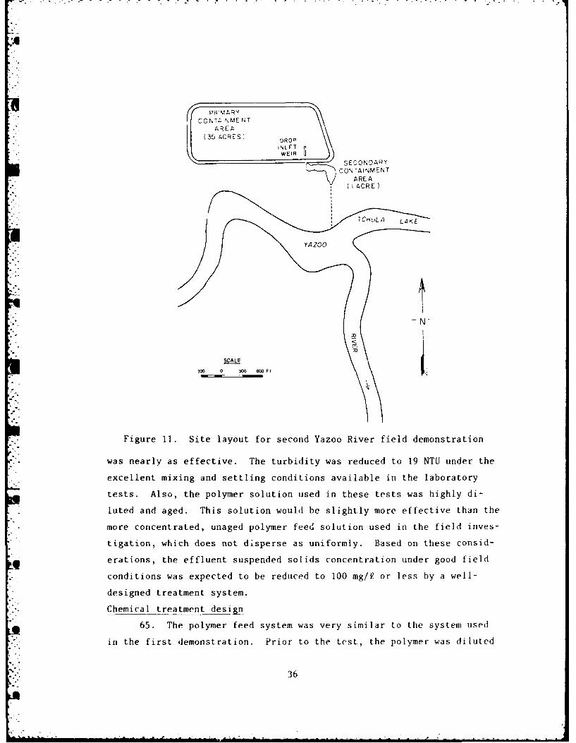
11 Site layout for second Yazoo River field demonstration 36
12 Suspended solids concentrations for secondYazoo River field demonstration ... .............. . 39
13 Site layout for Yellow Creek field demonstration ..... 41
14 Schematic of polymer feed system for Yellow Creekfield demonstration ....... .................... .. 43
15 Injection header for Yellow Creek field demonstration . . . 45
16 Suspended solids concentrations for Yellow Creekfield demonstration ....... .................... .. 47
17 Histogram of turbidity entering the secondary containmentarea, Yellow Creek field demonstration . .......... . 51
18 Histogram of secondary effluent turbidity, Yellow Creekfield demonstration ....... .................... .. 52
19 Turbidity data for long-term Yellow Creek fielddemonstration ........ ....................... ... 53
20 Sampling locations in secondary containment area, YellowCreek field demonstration ..... ................. .. 55
3
S . S -. U'- 'I -
No. Page
21 Polymer injection locations, Yellow Creek pipelineinjection field study ...... ................... ... 61
22 Schematic of polymer injection system, Yellow Creekfield study ........ ........................ . 62
23 Polymer loading for suspended solids removal by pipelineinjection, Yellow Creek field study .. ............ . 64
24 Polymer loading for turbidity removal by pipelineinjection, Yellow Creek field study .. ............ . 64
25 Flowchart of design procedures for chemical treatment . . . 69
26 Example weir mixing system .... ................ . 7727 Velocity gradient G calibration curves for jar test
apparatus ......................... 79
28 Nomograph relating design flow, weir length, effluentsuspended solids concentration, ponding depth, andweir loading for silts and saltwater clays . ......... 81
29 Nomograph relating design flow, weir length, effluentsuspended solids concentration, ponding depth, andweir loading for freshwater clays ... ............. . 82
30 Jar test report form ...... ................... . 86
31 Schematic of a simple liquid polymer feed system ..... 89
32 Schematic of a single tank liquid polymer feed system . . 90
33 Schematic of a two-tank liquid polymer feed system . . .. 90
34 Frontal view of a weir ..... .................. . 97
35 Example elevations in containment areas during. dewatering sequence ...... .................... ... 106
4
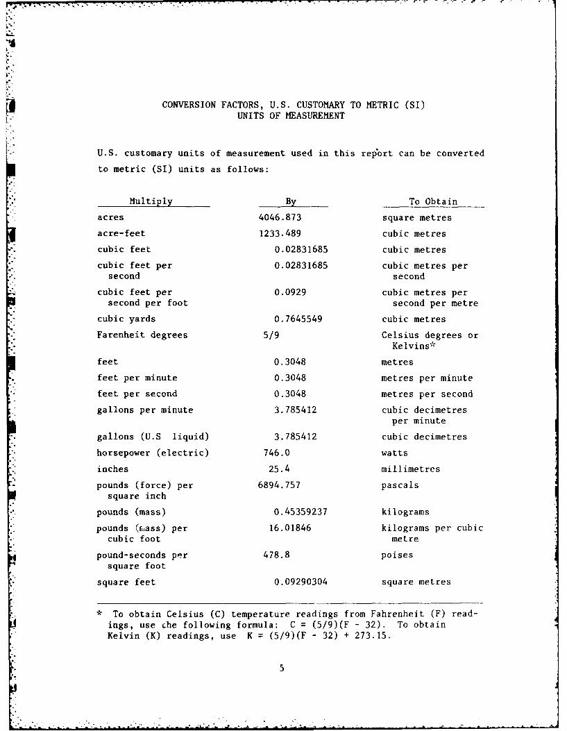
CONVERSION FACTORS, U.S. CUSTOMARY TO METRIC (SI)
UNITS OF MEASUREMENT
U.S. customary units of measurement used in this report can be converted
to metric (SI) units as follows:
Multiply By To Obtain
acres 4046.873 square metres
acre-feet 1233.489 cubic metres
cubic feet 0.02831685 cubic metres
cubic feet per 0.02831685 cubic metres persecond second
cubic feet per 0.0929 cubic metres persecond per foot second per metre
cubic yards 0.7645549 cubic metres
Farenheit degrees 5/9 Celsius degrees orKelvins*
feet 0.3048 metres
feet per minute 0.3048 metres per minute
feet per second 0.3048 metres per second
gallons per minute 3.785412 cubic decimetresper minute
gallons (U.S liquid) 3.785412 cubic decimetres
horsepower (electric) 746.0 watts
inches 25.4 millimetres
pounds (force) per 6894.757 pascalssquare inch
pounds (mass) 0.45359237 kilograms
pounds (n,ass) per 16.01846 kilograms per cubiccubic foot metre
pound-seconds per 478.8 poisessquare foot
square feet 0.09290304 square metres
* To obtain Celsius (C) temperature readings from Fahrenheit (F) read-ings, use che following formula: C = (5/9)(F - 32). To obtainKelvin (K) readings, use K = (5/9)(F - 32) + 273.15.
5
CHEMICAL CLARIFICATION METHODS FOR CONFINED
DREDGED MATERIAL DISPOSAL
PART I: INTRODUCTION
Background
1. The disposal of dredged material in confined disposal areas
has increased in recent years due to concern for the protection of the
aquatic habitat and water quality. The normal practice has been to pump
the dredged material as a slurry into a diked area where the material
settles out of suspension forming a settled dredged material layer and
supernatant water. The supernatant is then discharged over a weir and
*. returned to the waterway. Depending on the salinity of the water,
grain-size distribution of the material, and disposal site conditions,
the suspended solids concentration of the effluent for disposal of fine-
grained dredged material normally ranges between 200 mg/9. and 10 g/k.
* .Generally, well-designed containment areas should reduce the solids con-
centration to below 1 or 2 g/k. These effluent concentrations may ex-
ceed State or Federal water quality standards in certain areas; there-
fore, further treatment may be required to reduce the suspended solids,
settleable solids, or turbidity to meet the effluent standards.
2. The suspended solids and turbidity in the effluent from a con-
tainment area are colloidal material that does not readily settle by
gravity. Chemical clarification is one method to remove these fine par-
ticles from water. Many different chemicals are available which, when
added to the water, will aggregate the particles into a dense floc that
settles quickly. Efficient clarification requires optimum chemical
doses and mixing conditions for floc formation. Chemical clarification
is a treatment method primarily for the removal of suspended, not sol-
uble or dissolved, material from water.
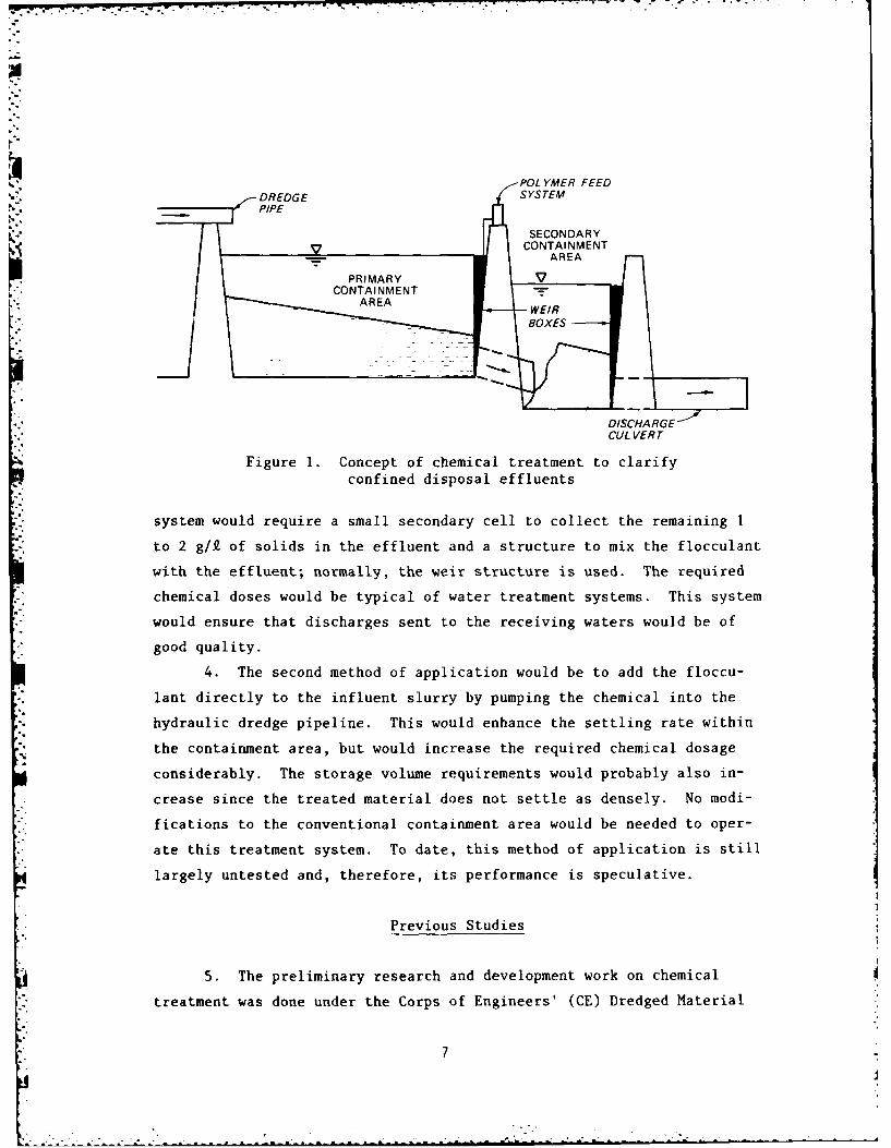
3. Chemical treatment can be applied at two points in the dis-
posal process. First, the treatment process can be used to polish the
effluent from the primary containment area as shown in Figure 1. This
6
POLYMER FEEDSRE-GE SYSTEMiFPIPE
~SECONDARY
V CONTAINMENT
PRIMARY ARE
CONTAINMENT-"
~~AREA WI
WEIR
DlSCHA RGE__.
CUL VERT
Figure 1. Concept of chemical treatment to clarify
confined disposal effluents
system would require a small secondary cell to collect the remaining 1
to 2 g/ of solids in the effluent and a structure to mix the flocculant
with the effluent; normally, the weir structure is used. The required
chemical doses would be typical of water treatment systems. This system
would ensure that discharges sent to the receiving waters would be of
good quality.
4. The second method of application would be to add the floccu-
lant directly to the influent slurry by pumping the chemical into the
hydraulic dredge pipeline. This would enhance the settling rate within
the containment area, but would increase the required chemical dosage
considerably. The storage volume requirements would probably also in-
crease since the treated material does not settle as densely. No modi-
fications to the conventional containment area would be needed to oper-
ate this treatment system. To date, this method of application is still
largely untested and, therefore, its performance is speculative.
Previous Studies
5. The preliminary research and development work on chemical
treatment was done under the Corps of Engineers' (CE) Dredged Material
7
Research Program (DMRP). Studies under the DMRP yielded many important
results. Wang and Chen (1977) examined the effectiveness of both con-
ventional coagulants and polymeric flocculants to treat dredged material
in jar tests. Over 50 chemicals were tested on sediments from five
sites. The sediments were diluted to simulate both slurries and super-
natants. The salinity of the samples was varied to determine its ef-
fect, but virtually all of the samples had sufficient salinity (greater
than 2 ppt) to behave as saltwater sediments. Conventional coagulants
(alum and ferric sulfate) were found to be unsuitable for treating
dredged material because of high dosage requirements, the need for pH
control, and the potential carryover of trace metals in the effluent.
Certain polymers worked excellently while others were ineffective even
at high concentrations. Anionic polymers were more effective on slur-
ries and high molecular weight, cationic polymers were best for super-
natants. The required polymer dosage increased with increasing initial
turbidity or solids concentration and decreased with increasing
salinity.
6. The study by Jones, Williams, and Moore (1978) develuped lab-
oratory procedures for determining the most effective polymer, the opti-
*mum dosage, and other design parameters for treating both slurries and
supernatants. They also provided guidelines on design procedures and on
operation of treatment systems. However, their designs were based on
using a conventional clarification system with conventional equipment
instead of incorporating the design into the normal containment area
conditions. Finally, they performed two field demonstration studies.
In one, the effluent from a freshwater dredged material containment area
was flocculated by three cationic polyelectrolytes in a conventional
physical-chemical pilot plant. The treatment system was very effective.
In the other study, a cationic polyelectrolyte was injected into the hy-
draulic dredge pipeline for a freshwater slurry. The results of the
test were erratic due to variations in flow and composition of the
dredged material slurry. Adding flocculant increased the settling rate
and reduced the supernatant turbidity; however, the supernatant of many
8
-% . .-- . . . " , . " - ". i ". . .' " • . . .; - " . . . "
samples was still very turbid. The use of flocculants to treat dredged
material was both simple and effective.
Purpose
7. The purpose of this report is to document the results of chem-
ical treatment demonstration projects and to provide guidelines for de-
sign and operation of chemical treatment facilities for clarification of
dredged material slurries and supernatants. Guidelines are presented on
sample collection and preparation, on laboratory tests to select a floc-
culant and to determine design parameters, and on the design and opera-
tion of the treatment system. This work evolved from preliminary
studies by Wang and Chen (1977) and by Jones, Williams, and Moore (1978)
and is intended to verify and to supplement their work.
8. The specific objectives of this study were as follows:
a. To verify the results and conclusions of previous studiessince only limited data were collected. The effectivenessof various flocculants for clarifying freshwater sedimentsneeded to be examined. Both methods of applying floccu-lants required additional field testing. Laboratory pro-cedures, design parameters, and design methods needed tobe compared with actual field conditions. The predictedeffectiveness of the treatment methods based on laboratorytests needed to be compared with the results of long-term,full-scale field tests.
b. To develop and evaluate treatment systems and methods toeffectively and efficiently treat primary containment areaeffluents and dredged material slurries. The methods andsystems developed in previous studies were traditional andwere not modified for the remote, temporary, and intermit-tent nature of dredging operations. The treatment systemmust be capable of handling high flow rates and highsolids loadings.
C. To simplify the selected treatment system for ease of6l operation. Due to the temporary nature of dredging,
trained, experienced operators are not available to run atreatment plant. Therefore, the system must be simple anddependable, requiring only minimum operation, maintenance,and supervision.
d. To reduce treatment costs. Simplification of the treatmentsystem reduces equipment and labor requirements and there-fore costs, but at the same time may increase chemical
-o9
9.'
.
usage and chemical costs. Costs can also be lowered byselecting the most cost-effective flocculant and bymaximizing its effectiveness in the treatment systemdesign.
e. To obtain information on treatment costs. Prior to thisstudy, the probable costs for treating dredged materialwere largely unknown.
f. To evaluate the removal efficiency of the selected treat-ment system. The effluent quality following chemicaltreatment had never been measured under normal field con-ditions. Therefore, the practical limitations of treat-ment needed to be determined.
g" To develop guidelines for laboratory testing to determinedesign parameters for the treatment method, and to developguidelines for the actual design and operation of thetreatment system. Treatment systems for dredged materialare quite different from typical water and wastewatertreatment plants because of the high sediment loads andthe temporary and intermittent operation associated withdredging projects. Therefore, specific guidelines areneeded for the design and operation of the treatment sys-tem. Also, the dredged material, the dredging operation,and the disposal site characteristics are unique. Conse-quently, laboratory tests that simulate field conditionsare required for each project to select a flocculant andto determine design parameters.
Scope
9. The general approach of this study was to design treatment
systems for the clarification of effluents or supernatants based on lab-
oratory tests and field conditions, and then to evaluate the performance
of the systems in full-scale field demonstrations. Specifically, three
demonstration sites were selected and sediment samples were collected.
Laboratory tests and procedures were developed and performed to prepare
suspensions of the sediments, select a flocculant, examine the effects
of mixing and settling conditions, establish minimum mixing and settling
requirements, select the required flocculant dosage, and obtain an esti-
mate of the achievable effluent quality. The project's treatment system
was designed and equipment was selected. The treatment system was set
up and field tested. The effluent quality was measured as a function of
dosage; the efficiency and adequacy of the mixing was evaluated; and the
10
practical limitations of turbidity and suspended solids removal were
determined. Operating experience was gained to develop operating guide-
lines, and the operation and maintenance requirements were established.
The available settling time in the secondary containment area was deter-
mined by dye tracer tests, and the adequacy of the settling conditions
was evaluated. The storage requirement for settled treated material was
." determined. Finally, the overall technical and economic feasibility was
examined, and recommendations were proposed.
10. A preliminary field investigation was also performed to eval-
uate the feasibility of injecting polymer directly into the dredge pipe-
line to treat dredged material slurries. Data were collected on the
settling rate of the slurry, on the turbidity and suspended solids con-
centration of the slurry prior to settling, and on the supernatant after
settling for 10 min. The effects of polymer dosing rate and location of
polymer injection on clarification were examined.
I
11
PART II: AGGREGATION OF DREDGED MATERIAL
11. This section presents a brief summary of background informa-
tion and theory on aggregation of dredged material. More detailed dis-
cussions and literature reviews were previously presented by Wang and
Chen (1977) and Jones, Williams, and Moore (1978). The advantages and
application of flocculation by polymers as compared with aggregation by
conventional aggregants* are also discussed herein.
12. In this report, the terms "aggregation," "coagulation," and
"flocculation" will be used in accordance with the system established by
La Mer (1964). "Aggregation" refers to any mechanism that causes col-
loidal particles to agglomerate. "Coagulation" is defined as electro-
static destabilization by the reduction of surface potential and charge
of the particles. "Flocculation" is destabilization by the chemical
bridging of colloidal particles by polmyers. The polymer adsorbs on the
particles forming a dense, three-dimensional floc that settles rapidly.
The terms "aggregants," "coagulants," and "flocculants" refer to the
chemicals that promote destabilization by the mechanism of aggregation,
coagulation, and flocculation, respectively. Colloidal stability is de-
fined as the property of particles to remain in suspension.
Properties and Behavior of Fine-Grained Material
13. The character of dredged material and its suspending medium
can strongly affect the settleability of the material and the selection
of an aggregant. Saltwater enhances settleability, but may chemically
react with the aggregant. The organic content of sediments and the ad-
sorbed ions and other substances on the particle surface may increase
0... the colloidal stability toward certain aggregation mechanisms. These
substances may also interact with aggregants and therefore restrict the
* .effectiveness of the treatment. Particle size affects the settling
* An aggregant is any chemical that promotes clarification and shouldnot be confused with an aggregate.
12
rate: coarse-grained material settles rapidly and does not require
chemical treatment to enhance settleability, while fine-grained mate-
rials, clays, are colloidal and require aggregation to achieve good
clarification in confined disposal containment areas.
14. At freshwater sites, the effluent quality from confined dis-
posal sites and the required aggregant dose to treat dredged slurries
and disposal effluents are strongly related to the concentration of
clays in the dredged slurry. This concentration depends on the concen-
tration of the dredged slurry and the clay content of the sediment. The
average solids concentration may vary from about 30 to 250 g/Q, but 145
g/2 is generally used as the norm. The particle-size distribution and
therefore the clay content also vary greatly.
15. Colloidal particles are stabilized mainly by two phenomena,
electrostatic repulsions and hydration. Clean sediments, free of solu-
ble organics, are normally stabilized by electrostatic forces resulting
from the net negative charge on the particles in an aqueous environment.
These sediments are the easiest to aggregate. They readily coagulate in
saltwater. Polymers are commercially available that will flocculate
this material at low dosages.
16. Organic clays and sediments with adsorbed organics are often
stabilized in part by hydration. The affinity of these organics for
water results in the formation of a sheath or shell of water molecules
that encapsulates the colloidal particle. This shell protects the par-
.ticles in two possible ways. First, the water acts as a mechanical bar-
rier that inhibits aggregation by preventing contact during particle
collisions. To penetrate this barrier, part of the solvent must be de-
sorbed from the surface, requiring energy to overcome the forces of hy-
dration. Dehydration is also required so that polymers can adsorb on
the particles. Second, it is also theorized that the water dipoles in
the shell are oriented by the surface charge. These oriented dipoles
repel dipoles similarly oriented on other particles as the two particles
approach each other. Suspensions that are stabilized by hydration are
more difficult to clarify. By practical means, they can be effectively
aggregated by two mechanisms: enmeshment in a precipitate or floc and
13
F J
flocculation by polymer with strong adsorption energies.
Aggregant Types and Descriptions
17. There are three main types of aggregants: simple salts,
hydrolyzable salts, and polymeric flocculants. Each type aggregates
colloidal suspensions in a different manner. Simple salts are the clas-
sical coagulants of the late 1800's and early 1900's. They were used in
the early quantitative studies conducted by Schulze, Hardy, and Freund-
lich (Alexander and Johnson 1949), which led to the Schulze-Hardy rule.
These salts, typically of sodium, potassitum, calcium, and barium, form
monovalent, divalent, and polyvalent ions of opposite charge to that of
the colloidal particles. The coagulants reduce the electrostatic repul-
sion between the particles.18. The hydrolyzable salts of iron and aluminum are the primary
aggregants used for treatment of surface water for drinking water sup-
plies. These salts interact with water to form many species, all in
equilibrium with each other. The dominant species varies as a function
. of pH. The optimum species for aggregation is the hydroxide precipitate
which predominates at neutral pH. Upon addition to water, the salt acts
as an acid, lowering the pH and requiring three hydroxides to neutralize
a free aluminum or iron ion. Therefore, pH adjustment may be necessary
to control the aggregation. The aggregants work by gathering the col-
loid in the hydroxide precipitate floc. At low pH, the aggregants can
coagulate colloidal particles in the same manner as simple salts.
19. Polymers are the newest type of aggregant. As more and more
kinds are synthesized, polymers are being used to treat all types of
waters and wastewaters. A polymer is composed of many small organic
subunits or monomers of one or more kinds linked in a recurring pattern
to form a chain. If these monomers have ionizable groups (e.g., car-
boxyl, amino, or sulfonic groups), the polymer is called a polyelectro-
lyte. Depending on its monomers, a polyelectrolyte may be either cat-
ionic, anionic, or ampholytic. Nonionic polymers contain no ionizable
groups. Polymers flocculate colloidal particles by forming a bond with
• 14

the particles or by neutralizing the charge on the particles.
Aggregation Mechanisms
20. The destabilization of colloidal suspensions can be accom-
plished by many different mechanisms. The mode of action is dependent
on the nature of the aggregant, the colloid, and the stability forces.
Suspensions of hydrophobic particles are aggregated primarily by reduc-
ing the electrical double layer repulsion, by chemical bridging or floc-
culation, and by enmeshing. The main methods for destabilizing suspen-
sions of hydrophilic particles are dehydration, precipitation, floccula-
tion, and enmeshment. Many colloids possess both hydrophobic and hydro-
philic properties and therefore the best aggregation mechanism is not
always readily apparent. Typically, dredged material would be hydropho-
bic, but it may possess some hydrophilic properties in the presence of
organic substances.
21. Simple coagulation is the destabilization of colloidal sus-
pensions by simple, nonpotential-determining ions. The counterions
(ions with the opposite charge of the particles) compress the diffused
electrical double layer surrounding the colloidal particles, lowering
the electrical repulsive potential and potential energy barrier. Conse-
quently, the van der Waals attractive forces become greater than the re-
pulsion and the particles aggregate. Compaction of the double layer is
dependent on both the concentration and charge of the counterions. The
coagulation follows the Schulze-Hardy rule, which states qualitatively
that the coagulating power of the coagulant increases greatly with the
counterion charge. The coagulation is nearly independent of the suspen-
sion concentration though the mechanism is more effective at high con-
centrations of particles. On a practical basis, the mechanism is too
slow for widespread application and Lhe particles can he easily redis-
persed. Also, high salt concentrations are generally required, which
would be undesirable in freshwater environments. In brackish and salt-
water regions, this coagulation mechanism occurs naturally.
22. A second mode of coagulation is adsorptive coagulat ion by
15
potential determining ions. In this case, the counterions are adsorbed
on the suspension particles, lowering or neutralizing the surface charge
and potential. Thus, the electrical repulsion potential is lowered
throughout the diffused layer allowing aggregation to occur. According
to Matijevi6 and Allen (1969), the main ionic species responsible for
adsorptive coagulation are large complex ions and odd-shaped ions such
as metal chelates with bulky ligands, organic ions of irregular shape
like surfactants and soaps, and some hydrolyzed metal ions. Other ions
that are constituents of the particles, such as hydrogen and hydroxide
ions for hydrolyzed particles, are also potential-determining and pro-
mote aggregation by the same mechanism (van Olphen 1963). Adsorptive
coagulation destabilizes the particles at lower coagulant doses than
predicted by the Schulze-Hardy rule. Often adsorptive coagulants at
higher concentrations restabilize the suspension by charge reversal.
The required coagulant dose, since the aggregation mechanism operates by
*adsorption, is dependent on suspension concentration, affinity for the
coagulant, and, only to a limited degree, on counterion charge.
23. A third mode of coagulation is the destabilization of parti-
cles by other particles. Heterocoagulation proceeds by the electrosta-
tic attraction of oppositely charged diffused layers and particles.
Mutual coagulation is the aggregation of particles of like charge. Clar-
ification occurs only at high suspension concentrations mainly due to
the increase in the particle collision frequency and floc formation.
This is the chief mechanism for the clarification of fine-grained fresh-
water materials in the primary containment area.
24. Enmeshing is a second method of destabilization, whereby col-
loidal particles are gathered in the precipitate of a metal salt. The
particles are then swept out of suspension as the precipitate settles.
The volume of precipitate greatly increases the sludge volume to bestored. Enmeshing is the principal mechanism for aggregation by the hy-
* drolyzable salts of iron and aluminum. With these aggregants, enmeshing
occurs in the neutral pH range at concentrations of metal salt above the
critical supersaturation point of the precipitate.
- "25. The final mechanism to be discussed is flocculation or
16
chemical bridging. Polymers or polyelectrolytes adsorb on suspension
particles forming bridges between them. The resulting dense, three-
dimensional floc settles rapidly entraining other colloidal particles
and effectively clarifying the liquid. Mixing is needed to promote con-
tact between polymer chains, particles, and flocs. The polymer, when
added at high concentrations, completely covers all of the adsorption
sites on the particles, preventing each polymer chain from adsorbing on
several particles and bridging. Thus, high polymer dosages protect the
particles from aggregation. Excessive high intensity mixing has a simi-
lar effect. The mixing shears the polymer from particles, breaking the
bridges between particles. The polymer then folds back onto the parti-
cle to which it is attached and adsorbs on several more sites on this
particle. This prevents the polymer from readsorbing on other particles
and forming bridges. The polymer also reduces the number of adsorption
sites on the particle available for anchoring other polymer chains.
Therefore, an optimum polymer dose and mixing condition exist for
flocculation.
Advantages of Polymers for Dredging Operations
26. The use of polymeric flocculants to chemically treat dredged
material offers many advantages over other aggregants. Liquid polymers
are less expensive to use and easier to handle and feed. They rapidly
produce a better quality effluent and work better within normal site
constraints. Many of these advantages were documented by Wang and Chen
(1977) and Jones, Williams, and Moore (1978) while others were identi-
fied in the chemical tr-atment demonstration projects reported herein.
These demonstrations verified the practicability, ease, and effective-
ness of using liquid polymers to treat dredged material supernatants.
27. Polymers aggregated dredged material supernatants at much
lower dosages than conventional inorganic aggregants in laboratory jar
tests. Optimum polymer dosages were generally about 8 ppm while about
49 200 ppm of the hydrated alum or ferric sulfate salts was required for
17

effective clarification. Polymers cost approximately $0.70/lb* and alum
or ferric sulfate about $0.05/lb, but because of the required dosages,
the chemical costs for polymers would be about half that for conven-
tional aggregants.
28. Liquid polymers and chemicals are easier and less expensive
to handle and feed. The only equipment needed is a storage tank, a di-
lution tank in some cases, and a metering pump. Dry chemicals require a
storage hopper with dust control, a dry chemical dispenser, a dissolving-
aging tank, a storage tank, and a metering pump. Besides the savings in
equipment, liquid chemicals have lower operation and maintenance costs.
At a dredging site, it is simpler to haul and store chemicals in a tank
or barrels than to handle dry chemicals and build a elevated storage
hopper. Another advantage of the smaller dosages for polymers is that
the quantity of chemicals to be hauled, handled, and fed is much less
than required for other aggregants.
29. Unlike alum or ferric salts, polymers do not require pH con-
trol to be effective. This eliminates the adition of lime or sodium
hydroxide, thereby reducing chemicals, equipment, and labor requirements
and their costs.
30. Flocculation by polymers is better suited for the mixing and
settling conditions present at dredged material disposal sites. Polymer
adsorbs rapidly and strongly, and works well under a wide variety of
mixing conditions though uniform mixing is preferable. This is impor-
tant because, typically, very little mixing time is available to promote
particle contact and floc formation. Also, the mixing intensity is dif-
ficult to control since mixing is normally provided by the weir struc-
ture between the primary and secondary areas. Under intense mixing, the
floc may shear, but the polymer is capable of rebuilding flocs many
times. These flocs continue to grow in the secondary settling basin and
then settle rapidly. The secondary basin normally provides I to 2 hr of
settling time with less than quiescent conditions, primarily due to wind.
A table of factors for converting U. S. customary units of measure-ment to metric (SI) is presented on page 5.
18
Polymer-flocculated material was not easily sheared and resuspended by
wind-induced turbulence during field tests. Other aggregants often have
more rigorous mixing and settling requirements. Also, material aggre-
gated by conventional aggregants and resuspended by wind in the second-
ary basin does not settle again as well as material treated with
polymers.
4
19
-. 4.
PART III: PRELIMINARY SCREENING OF AGGREGANTS
31. The initial work on evaluating the effectiveness of various
aggregants was conducted by Wang and Chen (1977). They cursorily tested
more than 40 aggregants on the supernatant of saltwater sediments with-
out performing jar tests. Instead, they used a nonstandard experimental
setup to examine the clarification of 200-NTU* suspensions by 4 ppm of
each polymer and of 1000-NTU suspensions by 8.5 ppm of each polymer.
Therefore, it was felt that a more extensive examination using jar tests
was warranted, particularly on freshwater sediments.
32. Forty-seven diverse aggregants were collected for testing.
Twelve of the polymers were eliminated at the start because of chemical
similarities. The remaining thirty-five chemicals were evaluated in the
laboratory. The polymers and their descriptions are listed in Table 1.
33. The initial screening was performed using freshwater clay
sediment from the Yazoo River channel modification project located near
Belzoni, Miss. Specific information on the properties of the sediment
is presented in Part IV with the background information on the first
demonstration project. Laboratory screening was performed in two
stages. In the first stage, the minimum and optimum aggregant dose was
determined by adding aggregant incrementally to a dredged material sam-
ple, mixing the sample, and observing the resulting floc formation and
clarification. In the second stage, the promising aggregants from the
initial screening were examined more closely by jar tests.
34. The initial screening was performed in several steps; each
successive step used a higher concentration of dredged material. After
each step, the results were evaluated and the aggregants demonstrating
inferior performance were rejected. The remaining aggregants were
tested further.
35. The initial concentrations of dredged material used in thetests were 0.21 and 0.42 g/£. A 1-£ sample was placed in a 1-k beaker
and mixed at 100 rpm on a standard Phipps and Bird jar test apparatus
NTU = Nephelometric Turbidity Units.
20
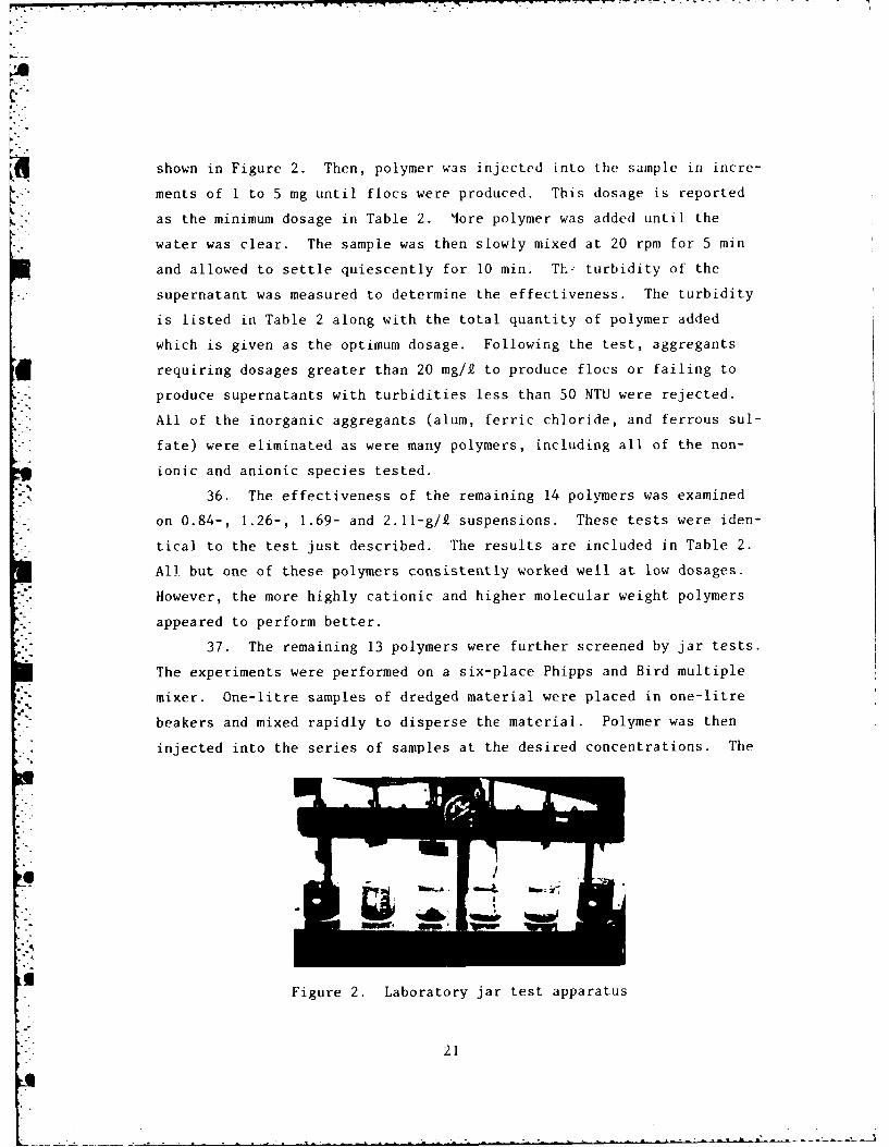
shown in Figure 2. Then, polymer was injected into the sample in incre-
ments of 1 to 5 mg until flocs were produced. This dosage is reported
as the minimum dosage in Table 2. 4ore polymer was added until the
water was clear. The sample was then slowly mixed at 20 rpm for 5 min
and allowed to settle quiescently for 10 min. Th- turbidity of the
supernatant was measured to determine the effectiveness. The turbidity
is listed in Table 2 along with the total quantity of polymer added
which is given as the optimum dosage. Following the test, aggregants
requiring dosages greater than 20 mg/2 to produce flocs or failing to
produce supernatants with turbidities less than 50 NTU were rejected.
All of the inorganic aggregants (alum, ferric chloride, and ferrous sul-
fate) were eliminated as were many polymers, including all of the non-
ionic and anionic species tested.
36. The effectiveness of the remaining 14 polymers was examined
on 0.84-, 1.26-, 1.69- and 2.11-g/k suspensions. These tests were iden-
tical to the test just described. The results are included in Table 2.
All but one of these polymers consistently worked well at low dosages.
However, the more highly cationic and higher molecular weight polymers
appeared to perform better.
37. The remaining 13 polymers were further screened by jar tests.
The experiments were performed on a six-place Phipps and Bird multiple
mixer. One-litre samples of dredged material were placed in one-litre
beakers and mixed rapidly to disperse the material. Polymer was then
injected into the series of samples at the desired concentrations. The
Figure 2. Laboratory jar test apparatus
21
samples were mixed at 100 rpm for 1 min to disperse the polymer and to
promote polymer-particles contact. A slow mix at 20 rpm for 5 min fol-
lowed to induce floc formation. The suspensions were allowed to settle
for 10 min. After settling, the supernatant was sampled at about 4 cm
beneath the surface and the turbidity was measured on a Hach Model 2100A
turbidimeter.
38. All polymers were tested on 0.5-g/k suspensions or the Yazoo
River sediment. The polymer dosage was varied from about 2 to 24 mg/f
in a series of samples. The results are listed in Table 3. All of the
polymers performed well, but half of the polymers were eliminated to
narrow the investigation to the best polymers. The seven polymers that
yielded the lowest turbidities at dosages of 16 and 20 mg/f were exam-
ined further.
39. Seven polymers were examined using jar tests with 1.0-g/9
suspensions. The polymer dosage ranged from 5 to 30 mg/k. Three of the
polymers worked very well and were tested on 2.0-g/f suspensions. Over-
all, Magnifloc 577C was the best, producing the clearest supernatant at
any dosage (Table 3).
40. Several other less intensive screening tests were performed
on other sediments using the proven performers of this screening and of
the studies by Wang and Chen (1977) and Jones, Williams, and Moore
(1978). The proven performers were limited to liquid polymers of low to
medium viscosity due to their ease of application in the field. These
polymers were Magnifloc 573C, 577C, and 581C; Nalcolyte 7103 and 7132;
9Calgon M-502; and Hercofloc 863. The polymers selected for the sedi-
ments are found in Table 4, and the project locations are shown in Fig-
ure 3. Recommended laboratory procedures for selecting a polymer are
presented in Part VI.
22
HARBOR__----
J~ ~
------------------------- - -----
L ------ -.- - M IG EE.4~ ESSERE~
COO PER IEYAZOO RIVERS
FORT CANAVERAL
Figure 3. Sediment sites for screening flocculants
23
PART IV: FIELD DEMONSTRATIONS OF TREATINGPRIMARY CONTAINMENT AREA EFFLUENTS
41. Three field demonstration projects were performed to test the
effectiveness and design of chemical treatment systems to clarify the
effluent from primary containment areas. The studies were also used to
evaluate the design procedures, to develop guidelines for operating the
systems, and to examine treatment costs. Two of the studies were con-
ducted on the Yazoo River and the third on Yellow Creek, Tennessee-
Tombigbee Waterway. The sediments at all three sites were freshwater
material with a significant fraction of clays. In absence of treatment,
effluent solids concentrations would have been greater than 1 g/P.
Therefore, these sites provided an opportunity to evaluate the treatment
method under strict conditions. Costs of the three demonstration proj-
ects are also discussed herein.
First Yazoo River Demonstration
Background
42. The demonstration was performed at disposal area No. I of
Upper Yazoo Project Item 2A-1 near Belzoni, Miss., on 28-29 Nov 1979,
with the support of the U. S. Army Engineer District, Vicksburg. The
previously f:lled and abandoned disposal area No. 6 of Item 1-C was ad-
jacent to the site and therefore was used as the secondary containment
area. The containment area layout is shown in Figure 4. The primary
containment area had a surface area of 48 acres and a depth of 12 ft.
The secondary area had a surface area of 43 acres, but only a third of
the area was ponded and then just to a depth of 1 to 2 ft. The two
areas were connected by a 120-ft fixed crest weir with a spillway that
fed the overflow directly into the secondary area.
43. The dredging activity was new construction work on a fresh-
water channel modification. Material dredged from the river banks was
about 85 percent fine-grained material, 35 percent clay, and was clas-
sified as a lean, sandy, silty clay (CL) with low plasticity. An 18-in.
hydraulic dredge was discharging about 27 cfs intermittently into the
primary area throughout the study.
24
w, .
+"" DREDGE.. DISCHARGE
DISPOSAL AREA NO. 1
.:: ,(PRIMARY
C ONTAINMEN!i AREA
T120-T WEI T
F 4 uITEM 1-C+? SECNDARY DISPOSAL AREA NO. 6
.. CONTAINMENT"-:'-''" tAREA
"' SCALE
."500 0 500 1000 FT
L ,-LOU:OUTLET BOX WEIRS
Figure 4. Layout of first Yazoo River field
demonstration site
25
44. The purpose of this study was to demonstrate that clarifica-
tion by polymer addition could be achieved with moderate doses of floc-
culant without a traditional treatment plant. This was the first at-
tempt to adapt the treatment process to the dredging operation.
Laboratory results
45. The polymer screening test described in Part III indicated
that Magnifloc 577C would be the best polymer. The required polymer
dosage, as determined by jar tests, was about 10 mg/k for a 1.0-g/Q sus-
pension, 15 mg/k for a 2.0-g/k suspension, and 25 mg/. for a 5.0-g/P
suspension. The effluent turbidity was less than 50 NTU when adequate
mixing and settling were provided. A minimum of I min of turbulent mix-|" -1ing at a mean velocity gradient G of 100 sec and 3 min of slow mix-
-Iing at a G of 20 sec was required for the polymer to be quite effec-
tive. Mean velocity gradient G is a measure of mixing intensity. Ten
minutes of settling provided sufficient time for clarification in the
;lboratory tests. The polymer was diluted in the laboratory tests to
several concentrations with either tap water or distilled water. No
difference in the effectiveness of the polymer was observed in jar tests
at the various polymer feed concentrations prepared with either type of
dilution water.
Chemical treatment design
46. Based on the laboratory results and project information, a
chemical treatment system was designed for a 2-day, full-scale demon-
stration. Three basic operations are performed in a chemical clarifica-
tion system: polymer addition, mixing, and settling. Each operation
was simplified to minimize equipment, labor, and power requirements, and
designs were developed to operate within the site constraints.
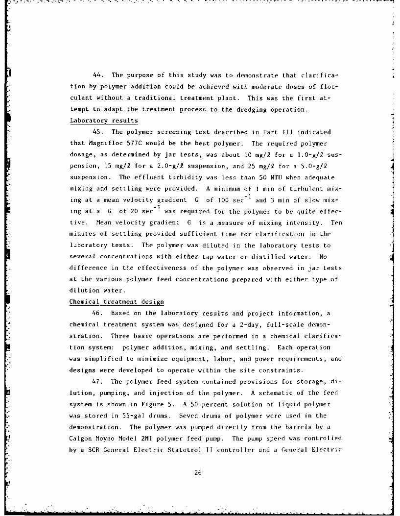
47. The polymer feed system contained provisions for storage, di-
lution, pumping, and injection of the polymer. A schematic of the feed
system is shown in Figure 5. A 50 percent solution of liquid polymer
was stored in 55-gal drums. Seven drums of polymer were used in the
demonstration. The polymer was pumped directly from the barrels by a
Calgon Moyno Model 2M] polymer feed pump. The pump speed was controlled
by a SCR General Electric SLatotrol II controller and a General Electric
26
U . . -.
k.7
WATER FROMCONTAINMENT AREA
WATER PUMP3 GPM
POSITIVE DISPLACEMENTMETERING PUMP
0.05-0.5 GPM
3-KW MOBILE P.. GENERATOR
115/240 V AC POLYMERSTORAGE
IN-LINEMIXER
• SPRAY HEADER- ., (FROM PVC PIPE)
Figure 5. Schematic of polymer feed system forYazoo River field demonstration
1/4-hp, variable speed, direct current (DC) motor. Power was supplied
by a 3-kw, portable, gasoline-powered generator (115/240-v alternating
current (AC)).
48. The polymer was diluted with the supernatant from the primary
containment area. Supernatant was pumped by a Calgon Moyno Model 2L3
polymer feed pump from a screened intake placed near the weir. The pump
was driven by a General Electric 3/4-hp, variable speed, DC motor con-
trolled by a SCR General Electric Statotrol II controller. The dilution
water was mixed with the polymer by an in-line mixer as the solution was
pumped to the injection rig through 3/4-in. rubber hose. The polymer
solution was not aged prior to being fed at a solution concentration of
about 6 percent or 60 g/k.
27
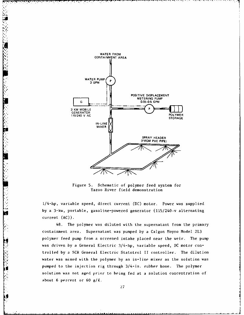
49. The injection system consisted of I-in. polyvinyl chloride
(PVC) pipe mounted on steel stanchions directly behind the weir crest.
Small holes were drilled on 2-ft centers along the entire length of the
pipe. The holes were oriented so that the polymer would be jetted into
the effluent as the water plunged over the weir. Figure 6 shows the in-
jection system in operation.
-°- , k.
Figure 6. Polymer injection header for firstYazoo River field demonstration
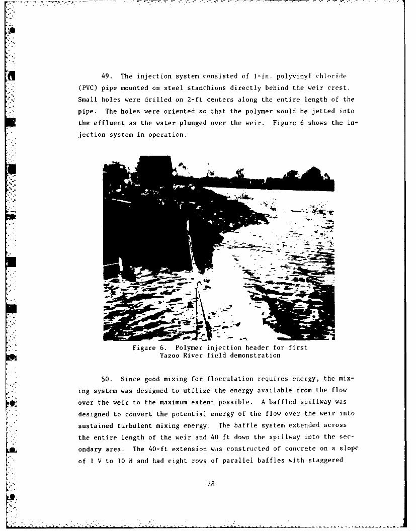
50. Since good mixing for flocculation requires energy, the mix-
- . ing system was designed to utilize the energy available from the flow
over the weir to the maximum extent possible. A baffled spillway was
designed to convert the potential energy of the flow over the weir into
sustained turbulent mixing energy. The baffle system extended across
the entire length of the weir and 40 ft down the spillway into the sec-
ondary area. The 40-ft extension was constructed of concrete on a slope
of I V to 10 H and had eight rows of parallel baffles with staggered
28
r ., ., . . .i . . - . .-. . -..
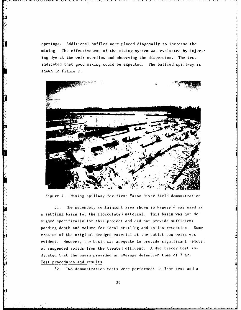
openings. Additional baffles were placed diagonally to increase the
mixing. The effectiveness of the mixing system was evaluated by inject-
ing dye at the weir overflow and observing the dispersion. The test
indicated that good mixing could be expected. The baffled spillway is
shown in Figure 7.
Figure 7. Mixing spillway for first Yazoo River field demonstration
51. The secondary containment area shown in Figure 4 was used as
a settling basin for the flocculated material. This basin was not de-
signed specifically for this project and did not provide sufficient
ponding depth and volume for ideal settling and solids retenti,n. Some
Serosion of the original dredged material at the outlet box weirs was
evident. However, the basin was adequate to provide significant removal
of suspended solids from the treated effluent. A dye tracer test in-
dicated that the basin provided an average detention time of 7 hr.
Test procedures and results
52. Two demonstration tests were performed: a 3-hr test and a
29
28-hr test. The short duration test was run to evaluate the effective-
ness of the injection and mixing prior to examining the entire design
and operation. Polymer was injected into the effluent for 3 hr at a
dosage rate estimated to be about 15 mg/2. The long duration test was
run to examine the effects of polymer addition on the suspended solids
concentration of the effluent from the secondary basin.
53. The exact polymer dosage was virtually impossible to deter-
mine due to difficulty in measuring the flow over the weir. The only
method available to determine the flow rate was to measure the depth of
flow over the weir and then compute the flow using standard weir for-4 -
mulas. The depth of the flow varied continuously due to wind-induced
waves. The flow rate also varied considerably due to the intermittent
operation of the dredge. The average depth of flow over the weir was
generally between I-1/4 and 1-1/2 in., corresponding to a flow rate of
about 20 cfs.
54. The effectiveness of the treatment was evaluated by running
batch settling tests on treated and untreated effluents. Samples of the
treated effluent were collected at the base of the spillway immediately
after the water passed through the baffles. The settling tests were run
in 1-2 graduated cylinders. Typical results for the treated effluent
are shown in Figure 8. The solids settled rapidly and nearly complete
clarification was achieved in less than 10 min. The untreated material
did not settle appreciably in the column and had not settled in the pri-
mary basin, which had a retention tire of several days. Figure 9 shows
a visual comparison of the treated and untreated samples following
10 min of settling. The tests indicated that the treatment system was
highly effective, but better results could be obtained if the mixing was
improved. Diagonal baffle boards were added to the spillway to increase
, the tortuosity and thereby the turbulence and mixing time.
55. The second demonstration test was run for 28 hr to examine
the effect of polymer addition on the suspended solids concentration of
the effluent from the secondary basin. The polymer dosing schedule and
test log for the demonstration are presented in the tabulation on
page 32. Polymer was pumped for the first 2 hr at a dosage of 12 mg/k
30
9
15
Z
I0
LaJ
II
" J"0
L I I
0 2 4 6 8 10
SETTLING TIME, MIN
:.- J iure' 8. S(ttI I rg results tor t retted,':xeffluent ill a 1-2 graltite.I ,l I yltr," first iazu)o River t ieH l(Terno)nst rat lull
--- I\
Figure 9. Batch settling tests of untreated and treatedeffluent samples, Yazoo River field demonstration
31
1~5.
bV W
Polymer Dosage
Hour Action mg/i
0 Started polymer pump and hourly samplers 12
2 Dredge stopped 15
4 Stopped polymer pump 0
6 Dredge started 0
8 Started polymer pump 15
10 Adjusted dosage 12
20 Adjusted dosage 15
23.5 Adjusted dosage 24
25 Adjusted dosage 20
27.5 Stopped polymer pump and samplers 0
based on a flow rate of 20 cfs. At this time, the dredge stopped for
4 hr and the flow rate had slowed to about 5 cfs when the dredge started
again. Between the second and fourth hours, the polymer dosage averaged
about 15 mg/ due to the decreasing flow. Due to the low flow rate, the
polymer pumps were turned off for the next 4 hr. Upon resuming opera-
tion, the dosage averaged about 15 mg/k for 2 hr at which time the flow
over the weir returned to about 20 cfs. Between the tenth and twentieth
S.hours, polymer was fed at a dosage of 12 mg/9. The dosage was then suc-
cessively increased to 15 mg/9 for 3-1/2 hr, to 24 mg/9 for 1-1/2 hr,
and 20 mg/£ for 2-1/2 hr. A total of seven barrels (about 320 gal) of a
* ". 50 percent polymer were used in the test.56. Samples were collected every hour at the primary weir and at
both box weirs in the secondary basin. The influent and effluent sus-
pended solids concentrations are plotted as a function of time in Fig-
ure 10. The reported effluent concentration is an average of the re-
sults at both box weirs. The initial effluent concentration was greater
than the influent concentration due to erosion near the outlet weirs.
57. The effluent suspended solids concentration started to de-
crease after 5 hr and to level off after 19 hr. The (lye tracer curve
showed that the peak dye concentration arrived at the discharge weirs
about 5 hr after injection at the primary weir. The mean retention time
was about 7 hr. Therefore, it required about 18 hr to completely flush
32S-"
- . . . . . . - . * * . . - . . a a . a *
4
3 INFLUENT
..
02
0
r0 4 8 12 16 20 24 28
TIME, HR
Figure 10. Hourly suspended solids concentrations for firstYazoo River field demonstration
the basin and to reach the steady effluent quality for any level of
"" treatment. The suspended solids concentration decreased steadily until
." the ninth hour when the concentration increased slightly and then re-
mained nearly constant for 4 hr. This began 5 hr after the polymer ad-
dition was stopped and lasted for the same duration as the stoppage.
Clearly, it was a result of stoppage. The suspended solids concentra-
tion was reduced further between the thirteenth and nineteenth hours.
The effluent quality then levelled off until. the twenty-fourth hour when
the solids level declined slightly. The last samples were collected
27 hr after the start of the test.
58. The data show that the steady-state effluent solids conc:en-
tration for a 12-mg/kZ polymer dosage was 650 ing/.Q. This corresponds to
a 77 pretreduction in speddsolids. Data weenot taken to
',-' idetermine the suspended solids removal at the higher dosages used at the
33
%..
end of the tests, but the solids concentration was decreasing at the
- end. At 8 hr after dosing at 15 mg/P, the suspended solids concentra-
tion was 450 mg/2, corresponding to a 83 percent reduction. It is
likely that better removals could have been attained if higher dosages
had been applied for longer periods and if the secondary basin had been
modified to provide more ideal settling conditions.
59. The demonstration was also used to develop operational proce-
dures and to identify operational and design problems. The project de-
monstrated that reliable power, good equipment, and regular maintenance
are needed to ensure good operation. Small portable generators cannot
. be expected to run for extended periods. The system should be checked
periodically and adjusted to account for changing flow rates and in-
fluent solids concentration. A better source of dilution water must be
used since the water in the primary basin was too dirty and contained
dead vegetation that clogged the screened intake and the holes in the
injection pipe. Vehicular access must be available to the treatment
site. Due to the intermittent operation of the dredge, the polymer feed
must be able to operate at very low flows or else the discharge weir
must be operable to increase the flow rate or stop the discharge.
Conclusions
60. The following conclusions were drawn:
a. The treatment system was highly effective though the re-movals were not as great as obtained in the laboratory.
b. The overall design concept was sound.
c. Sufficient energy was available from the difference inelevation between the water surfaces of the two basins tomix the effluent and polymer.
d. Other weir designs may improve the mixing.
e. The secondary basin must be designed to provide bettersettling conditions.
Second Yazoo River Demonstration
Background
61. The demonstration was performed at containment area No. 3 of
Upper Yazoo Project Item 2A-1 near Belzoni, Miss., on 9-12 June 1980
34
!
.- 7- T 7
with the support of the Vicksburg District. The containment at?a layout
is shown in Figure 11. The primary area had a surface area of 35 acres
and a depth of about 12 ft. An irregularly shaped secondary area was
constructed for the demonstration in a depression adjacent to the pri-
mary area. The area had a surface area of I acre and an average depth
of about 4 ft. The outlet from the primary cell was a rectangular fixed
crest drop inlet weir structure situated 20 ft into the basin. The
structure was 56 ft long and 4 ft wide and constructed of sheet metal
except for one 4-ft side that was boarded for use in dewatering. The
effluent was discharged from the weir to the secondary cell through a
100-ft-long, 24-in.-diam corrugated metal culvert. The difference in
elevation between the water surfaces of the two basins was about 12 ft.
62. An 18-in. hydraulic dredge was widening a channel and pumping
the material into the area. The mainly fine-grained dredged material
was a freshwater lean sandy silty clay (CL) with low plasticity as was
the sediment in the first demonstration. The flow averaged about 25 cfs
during the test.
63. This demonstration differed from the first test in three
ways. First, the weir structure was not modified to improve mixing.
Adequate mixing was available from the 12-ft drop between the areas and
the turbulence of the flow through the 100-ft-long corrugated metal cul-
vert. Eliminating the construction of a mixing system greatly reduced
the cost of treatment. The only additional construction required for
chemical treatment was that of a secondary containment area. Second,
the secondary area provided good settling conditions. Finally, the
polymer dosages were reduced to lower treatment costs. The demonstra-
tion examined the effectiveness of mixing in existing weir structures
and of lower polymer dosages with good mixing and settliaig conditions.
Laboratory results
64. Magnifloc 577C had been selected as the best flouluit for
Yazoo River material in the first demonstation and therefore was se-
lected for use in this test. Jar tests were run on 2-g/P suspensions
to determine the required polymer dosage and to estimate the achievable
reduction in turbidity. The optimum dosage was 6 mg/2, through 4 mg/k
35
iJ j
°6
• CONT INV E NT
. ARE A
• (35 ACRE S )DROP
IR
SECONDARYCONTAINMENTi. ( ARE )
I ARE
.'.- YAZOO
."'
SCALE FT
Figure 11. Site layout for second Yazoo River field demonstration
was nearly as effective. The turbidity was reduced to 19 NTU under the
excellent mixing and settling conditions available in the laboratory
tests. Also, the polymer solution used in these tests was highly di-
luted and aged. This solution would be slightly more effective than the
more concentrated, unaged polymer feed solution used in the field inves
tigation, which does not disperse as uniformly. Based on these consid-
erations, the effluent suspended solids concentration under good field
conditions was expected to be reduced to 100 mg/Q or less by a well-
designed treatment system.
Chemical treatment design
65. The polymer feed system was very similar to the system used
in the first demonstration. Prior to the test, the polymer was diluted
36
to one-third strength and then stored in twelve 55-gal drums. The poly-
mer was fed directly from the drums and diluted in line to a 4 percent
or 40-g/R aolution. The pumps, generator, and dilution water intakeI -
were the same as described for the first demonstration. The injection
rig was a closed loop of 1-in. PVC pipe mounted on the weir box along
the weir crest. The polymer was injected down into the weir box through
small holes drilled on 2-ft centers along the loop.
t)b. A mixing system was not designed for this demonstration. The
only fllxiri) provided was from the turbulence of the flow through the
weir structure. This corresponded to mixing at about a mean velocity
gradient G of 950 sec for about 13 sec. The weir structure provided
" 'excellent rapid mixing but no slow mixing. Slow mixing resulted only
from the advective currents in the secondary area.
67. The 1-acre secondary area shown in Figure 11 was used as a
settling basin for the treated material. A dye tracer test indicated
that the basin provided an average of 60 min of settling time and a min-
imum of 25 min. The basin had sufficient ponding depth and volume for
good settling and solids retention.
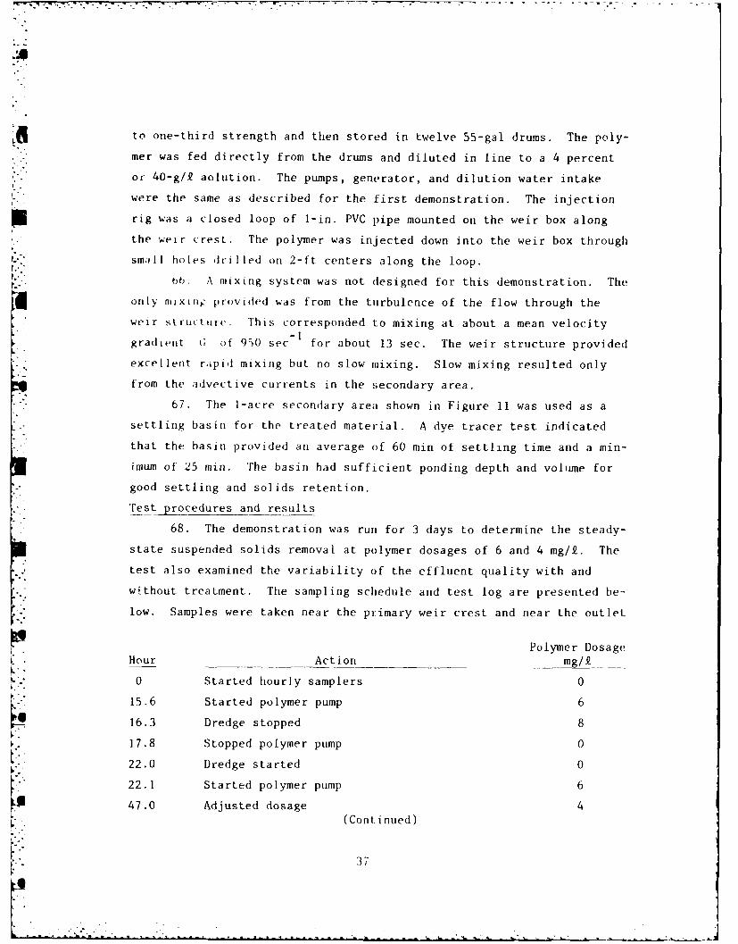
Test procedures and results
68. The demonstration was run for 3 days to determine the steady-
state suspended solids removal at polymer dosages of 6 and 4 mg/£p. The
test also examined the variability of the effluent quality with and
- . without treatment. The sampling schedule and test log are presented be--
low. Samples were taken near the primary weir crest and near the outlet
Polymer Dosage
Hour Action mg_J
0 Started hourly samplers 0
15.6 Started polymer pump 6K. 16.3 Dredge stopped 8
17.8 Stopped polymer pump 0
22.0 Dredge started 0
22.1 Started polymer pump 6
47.0 Adjusted dosage 4(Cont inued)
S"3 7
Polymer Dosage
Hour Action mg/.9
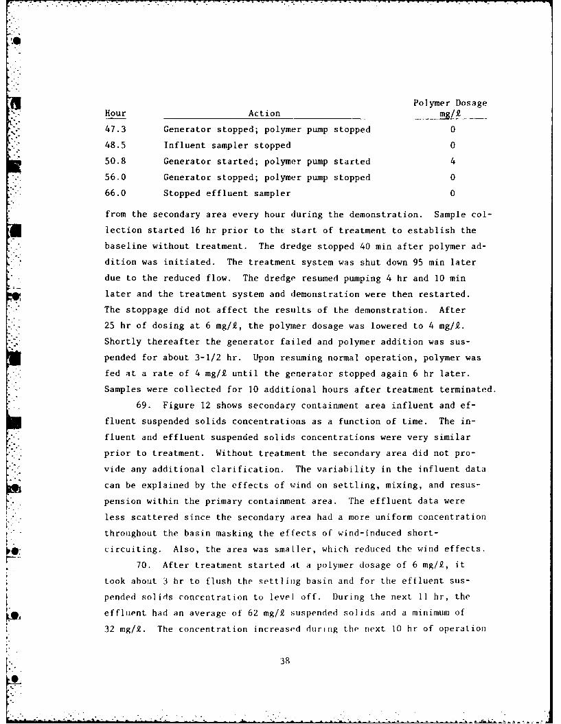
47.3 Generator stopped; polymer pump stopped 0
48.5 Influent sampler stopped 0
50.8 Generator started; polymer pump started 4
56.0 Generator stopped; polymer pump stopped 0
66.0 Stopped effluent sampler 0
from the secondary area every hour during the demonstration. Sample col-
lection started 16 hr prior to the start of treatment to establish the
baseline without treatment. The dredge stopped 40 min after polymer ad-
dition was initiated. The treatment system was shut down 95 min later
due to the reduced flow. The dredge resumed pumping 4 hr and 10 min
later and the treatment system and demonstration were then restarted.
-- The stoppage did not affect the results of the demonstration. After
* -' 25 hr of dosing at 6 mg/k, the polymer dosage was lowered to 4 mg/k.
-. ' Shortly thereafter the generator failed and polymer addition was sus-
pended for about 3-1/2 hr. Upon resuming normal operation, polymer was
fed at a rate of 4 mg/k until the generator stopped again 6 hr later.
Samples were collected for 10 additional hours after treatment terminated.
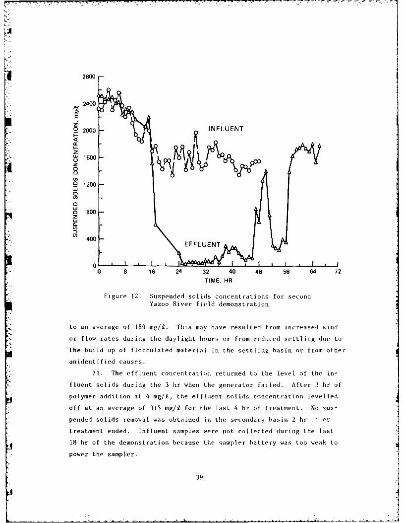
69. Figure 12 shows secondary containment area influent and ef-
fluent suspended solids concentrations as a function of time. The in-
fluent and effluent suspended solids concentrations were very similar
prior to treatment. Without treatment the secondary area did not pro-vide any additional clarification. The variability in the influent data
can be explained by the effects of wind on settling, mixing, and resus-
pension within the primary containment area. The effluent data were
less scattered since the secondary area had a more uniform concentration
throughout the basin masking the effects of wind-induced short-
circuiting. Also, the area was smaLler, which reduced the wind effects.
70. After treatment started at a polymer dosage of 6 mg/Q, it
took about 3 hr to flush the settling basin and for the effluent sus-
pended solids concentration to level off. During the next 11 hr, the
effluent had an average of 62 mg/k suspended solids and a minimum of
32 mg/Q. The concentration increased during the next 10 hr of operation
39
2800
2400
E
0 2000 INFLUENT
I--
u 1600zo P0
9 1200
0.-,
- 800Z
"" O3400400 EFFLUENT
00 8 16 24 32 40 48 56 64 72
TIME, HR
Figure 12. Suspended solids concentrations for secondYazoo River field demonstration
to an average of 189 mg/2. This may have resulted from increased wind
or flow rates during the daylight hours or from reduced settling due to
the build up of flocculated material in the settling basin or from other
unidentified causes.
71. The effluent concentration returned to the level of the in-
fluent solids during the 3 hr when the generator failed. After 3 hr of
polymer addition at 4 mg/R, the effluent solids concentration levelled
off at an average of 315 mg/k for the last 4 hr of treatment. No sus-
pended solids removal was obtained in the secondary basin 2 hr . er
treatment ended. Influent samples were not collected during the last
18 hr of the demonstration because the sampler battery was too weak to
power the sampler.
3.
----- ~ --------------------
72. During the period when the polymer dosage was 6 mg/R, the in-
fluent averaged 1555 mg/Q and the effluent averaged 120 mg/k. This cor-
responds to a 92 percent removal of suspended solids from the primary
effluent by the treatment process. For polymer addition at 4 mg/i,
about 80 percent of suspended solids was removed.
Conclusions
73. The treatment system was highly effective, with greater re-
ductions in suspended solids at significantly lower dosages than ob-
tained in the first field test. The better removals resulted from the
more intense mixing, greater mixing energy, lower influent suspended
solids concentrations, and better settling conditions present in this
study. However, these removals were slightly lower than anticipated
from the laboratory tests. The required polymer dosage may have been
slightly higher than determined by jar tests. More dilute and aged
polymer feed solutions like those used in the laboratory tests may have
been more effective. Better removals may also have been achieved if
slow mixing had been provided. Finally, the demonstration again showed
the importance of reliable, rugged equipment.
Yellow Creek Embayment Demonstration
Background
74. A full-scale, long-term demonstration was performed with the
support of the Nashville District as part of a maintenance dredging proj-
ect on the Tennessee-Tombigbee Waterway. The project was located at the
Yellow Creek Embayment of Pickwick Reservoir on the Tennessee River near
Burnsville, Miss. The layout of the site is shown in Figure 13. The
effluent from the primary containment area was treated for the entire
duration of the project running from early March 1981 to early June 1981.
Chemical treatment was required to meet the strict effluent quality re-
quirements of the project. The maximum allowable effluent turbidity
and suspended solids concentration were 100 NTU and 100 mg/Q, respec-
tively. In addition, the weekly average effluent turbidity was not to
exceed 50 NTU.
40
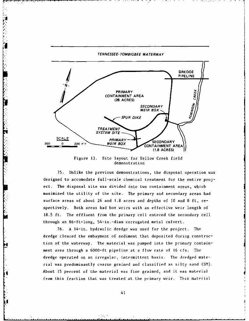
TENNESSEE- TOMBIGBEE WATERWAY
DEDGII PIPELINE
PRIMARY200 0 200FTWERO CONTAINMENT A REA/// ~(26 ACRES) /'/
~SECONDARY 0 1
•SPUR DIKE
k""Figure 13. Site layout for Yellow Creek field
~demonstration
"-"75. Unlike the previous demonstrations, the disposal operation was
i'- designed to accomodate full-scale chemical treatment for the entire proj-
ect. The disposal site was divided into two containment areas, which
i maximized the utility of the site. The primary and secondary areas had
surface areas of about 26 and 1.8 acres and depths of 10 and 8 ft, re-
spectively. Both areas had box weirs with an effective weir length of
18.5 ft. The effluent from the primary cell entered the secondary cell
through an 86-ft-long, 54-in.-diam corrugated metal culvert.
76. A 14-in, hydraulic dredge was used for the project. The
dredge cleared the embayment of sediment that deposited during construc-.1
4 tion of the waterway. The material was pumped into the primary contain-
ment area through a 6000-ft pipeline at a flow rate of 16 cfs. The
dredge operated on an irregular, intermittent basis. The dredged mate-
rial was predominantly coarse grained and classified as silty sand (SM).
( About 15 percent of the material was fine grained, and it was material
from this fraction that was treated at the primary weir. This material
41
4
was classified as a highly plastic clay (CH).
77. The objectives of this demonstration were multifold:
a. To examine further the available mixing in a conventionalweir structure.
b. To investigate the effect of polymer dosage un effluentquality over a wider range of dosages.
c. To establish the practical limitations of the treatmentsystem.
d. To determine the effluent quality that can normally beachieved.
e. To evaluate the long-term performance of the system.
f. To acquire long-term operating experience.
g. To establish operating guidelines.
h. To determine the storage volume required for flocculatedmaterial.
i. To determine typical chemical treatment costs.
Laboratory results
78. The sediment contained a large fraction of coarse-grained
material. Therefore, the samples were sieved through a U.S. Standard
No. 40 sieve prior to laboratory testing. Jar tests were then run on
2-g/£, suspensions of the sieved material. This material still contained
a significant portion of settleable material since 60 percent of the
material settled in the test without any polymer addition.
79. Four polymers were screened by jar tests: Hercofloc 863,
"agnifloc 577C, Nalcolyte 7103, and Calgon M-502. Each of these poly-
mers had performed well on other freshwater sediments. The jar tests
were run using 20 sec of rapid mixing at 100 rpm, 5 min of slow mixing
at 20 rpm, and 10 min of settling. Hercofloc 863 was selected as the
most cost-effective polymer though all four polymers performed equally
well. A 90 percent reduction in solids concentration was achieved with
a polymer dosage of 4 to 6 mg/k, and higher removals were obtained with
better mixing. The effluent water quality criteria were not met in the
tests, but the criteria were not established until after the screening
* was completed.
42
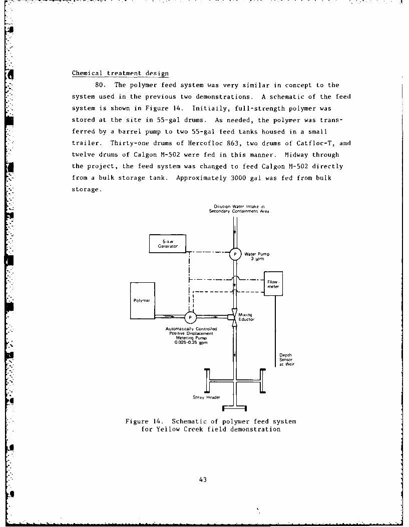
Chemical treatment design
80. The polymer feed system was very similar in concept to the
system used in the previous two demonstrations. A schematic of the feed
system is shown in Figure 14. Initially, full-strength polymer was
stored at the site in 55-gal drums. As needed, the polymer was trans-
ferred by a barrel pump to two 55-gal feed tanks housed in a small
trailer. Thirty-one drums of Hercofloc 863, two drums of Catfloc-T, and
twelve drums of Calgon M-502 were fed in this manner. Midway through
the project, the feed system was changed to feed Calgon 11-502 directly
from a bulk storage tank. Approximately 3000 gal was fed from bulk
storage.
Dilution Water Intake inSecondary Containment Area
- "5-k w, . GeneratorP Water Pump
3 ,pm
Flow-meter
P Mixing
' '.--. Eductor
Automatically ControlledPositive Displacement
Metering Pump0.025-0.25 gpm
DepthSensorat Weir
Spray Header
Figure 14. Schematic of polymer feed systemfor Yellow Creek field demonstration
43
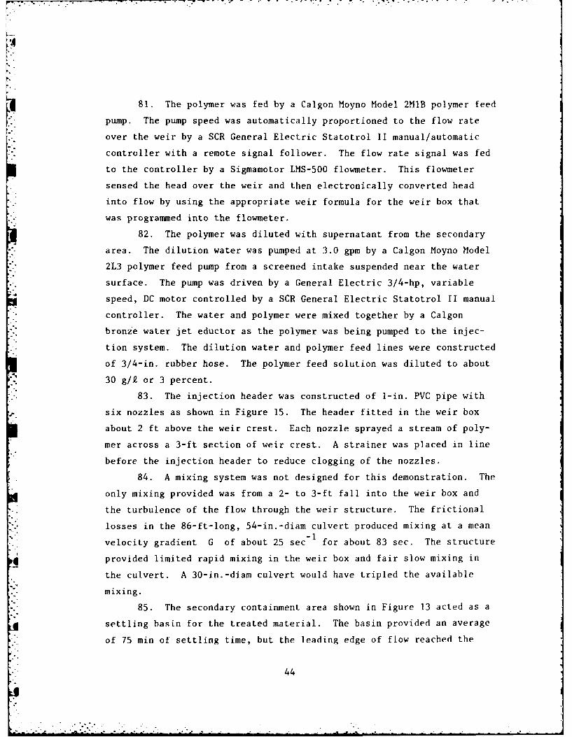
81. The polymer was fed by a Calgon Moyno Model 2MIB polymer feed
pump. The pump speed was automatically proportioned to the flow rate
over the weir by a SCR General Electric Statotrol II manual/automatic
controller with a remote signal follower. The flow rate signal was fed
to the controller by a Sigmamotor LMS-500 flowmeter. This flowmeter
sensed the head over the weir and then electronically converted head
into flow by using the appropriate weir formula for the weir box that
was programmed into the flowmeter.
82. The polymer was diluted with supernatant from the secondary
area. The dilution water was pumped at 3.0 gpm by a Calgon Moyno Model
2L3 polymer feed pump from a screened intake suspended near the water
surface. The pump was driven by a General Electric 3/4-hp, variable
speed, DC motor controlled by a SCR General Electric Statotrol II manual
controller. The water and polymer were mixed together by a Calgon
bronze water jet eductor as the polymer was being pumped to the injec-
tion system. The dilution water and polymer feed lines were constructed
of 3/4-in. rubber hose. The polymer feed solution was diluted to about
30 g/k or 3 percent.
83. The injection header was constructed of 1-in. PVC pipe with
six nozzles as shown in Figure 15. The header fitted in the weir box
about 2 ft above the weir crest. Each nozzle sprayed a stream of poly-
mer across a 3-ft section of weir crest. A strainer was placed in line
before the injection header to reduce clogging of the nozzles.
84. A mixing system was not designed for this demonstration. The
only mixing provided was from a 2- to 3-ft fall into the weir box and
the turbulence of the flow through the weir structure. The frictional
losses in the 86-ft-long, 54-in.-diam culvert produced mixing at a mean-1
velocity gradient G of about 25 sec for about 83 sec. The structure
provided limited rapid mixing in the weir box and fair slow mixing in
the culvert. A 30-in.-diam culvert would have tripled the available
mixing.
85. The secondary containment area shown in Figure 13 acted as a
settling basin for the treated material. The basin provided an average
of 75 min of settling time, but the leading edge of flow reached the
44
POLYMER FEED SYSTEM
'" 'PRESSURE GAGE
s yn 3SPRA Y
---- -----
' - WEIR
~BOX
• Figure 15; Injection header for Yellow Creekh. field demonstration
secondary weir in just 13 min. Considerable short-circuiting occurred,
but the basin had sufficient volume and detention time for good settling
and solids retention. The secondary cell provided enough storage for
only half of the flocculated material generated during the project.
Therefore, a 6-in., diesel-powered water pump was used periodically to
remove settled material from the secondary cell and to place it in the
primary cell.
86. The pumps, flowmeter, tools, and supplies were housed in a
small trailer parked on the dike between the primary weir box and the
inlet to the secondary cell. The trailer also provided shelter for the
operators. The equipment and trailer were initially powered by a 5-kw,
gasoline-powered Kohler generator. The generator failed after about 6
to 8 weeks of operation, and the power supply was switched to a diesel-
powered light plant.
45
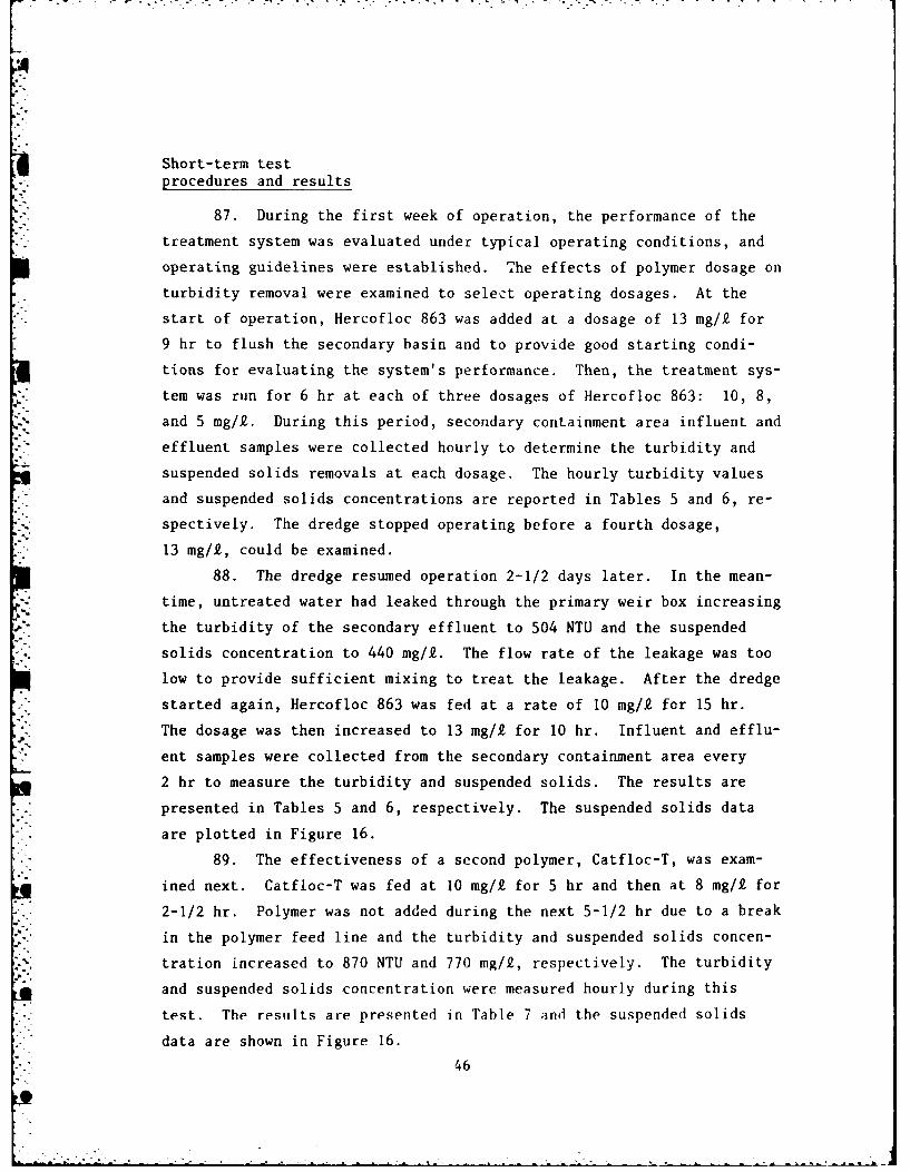
Short-term test
procedures and results
87. During the first week of operation, the performance of the
treatment system was evaluated under typical operating conditions, and
operating guidelines were established. The effects of polymer dosage on
turbidity removal were examined to select operating dosages. At the
start of operation, Hercofloc 863 was added at a dosage of 13 mg/k for
9 hr to flush the secondary basin and to provide good starting condi-
tions for evaluating the system's performance. Then, the treatment sys-
tem was run for 6 hr at each of three dosages of Hercofloc 863: 10, 8,
and 5 mg/i. During this period, secondary containment area influent and
effluent samples were collected hourly to determine the turbidity and
suspended solids removals at each dosage. The hourly turbidity values
and suspended solids concentrations are reported in Tables 5 and 6, re-
spectively. The dredge stopped operating before a fourth dosage,
13 mg/k, could be examined.
88. The dredge resumed operation 2-1/2 days later. In the mean-
time, untreated water had leaked through the primary weir box increasing
the turbidity of the secondary effluent to 504 NTU and the suspended
solids concentration to 440 mg/i. The flow rate of the leakage was too
low to provide sufficient mixing to treat the leakage. After the dredge
started again, Hercofloc 863 was fed at a rate of 10 mg/£ for 15 hr.
The dosage was then increased to 13 mg/£ for 10 hr. Influent and efflu-
ent samples were collected from the secondary containment area every
2 hr to measure the turbidity and suspended solids. The results are
presented in Tables 5 and 6, respectively. The suspended solids data
are plotted in Figure 16.
89. The effectiveness of a second polymer, Catfloc-T, was exam-
ined next. Catfloc-T was fed at 10 mg/k for 5 hr and then at 8 mg/2 for
2-1/2 hr. Polymer was not added during the next 5-1/2 hr due to a break
in the polymer feed line and the turbidity and suspended solids concen-tration increased to 870 NTU and 770 mg/Q, respectively. The turbidity
and suspended solids concentration were measured hourly during thistest. The results are presented in Table 7 and the suspended solids
data are shown in Figure 16.
46
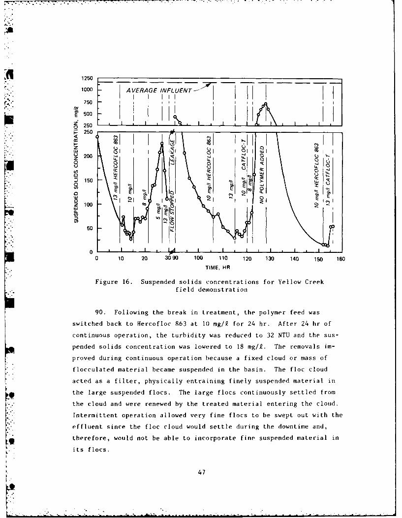
1250
1000 AVERAGE INFLUENT-
750 I ImE 500 -
Z'I~ I I r I I 'I0 250 , I2 250
S200 0
0
Z cc
z100 00 2 30 0 1
(n E
50 _-jL
0 10 20 3090 100 110 120 130 140 150 160TIME, HR
Figure 16. Suspended solids concentrations for Yellow Creekfield demonstration
90. Following the break in treatment, the polymer feed was
switched back to Hercofloc 863 at 10 mg/2 for 24 hr. After 24 hr of
continuous operation, the turbidity was reduced to 32 NTU and the sus-
pended solids concentration was lowered to 18 mg/),. The removals im-
proved during continuous operation because a fixed cloud or mass of
flocculated material became suspended in the basin. The floc cloud
acted as a filter, physically entraining finely suspended material in
* Othe large suspended flocs. The large flocs continuously settled from
the cloud and were renewed by the treated material entering the cloud.
Intermittent operation allowed very fine flocs to be swept out with the
effluent since the floc cloud would settle during the downtime and,
therefore, would not be able to incorporate fine suspended material in
its flocs.
47
rL. O
91. The polymer feed was changed to 13 mg/k Catfloc-T following
the 24 hr at 10 mg/k Hercofloc 863. This test was the last examining
the effect of polymer dosage and type, and ended after 4 hr when the
dredge stopped for maintenance. Effluent samples were collected hourly.
The results are reported in Table 7 and the suspended solids are plotted
in Figure 16.
92. Suspended solids and turbidity results for the tests are sum-
marized below. It was found that: (a) significant removals occurred at
all polymer dosages examined, (b) experiments on treated suspensions in-
dicated that better removals could have been obtained with better mix-
ing, (c) Hercofloc 863 performed slightly better than Catfloc-T, (d) the
required dosage was 10 mg/k, and (e) treatment at this polymer dosage
produced an effluent which, under normal conditions, satisfied the ef-
fluent quality requirements.
Polymer Turbidity Suspended SolidsDosage, mg/£ Removal, percent Removal, percent
Hercofloc 863
5 81.8 84.1
8 91.5 93.5
10 95.5 96.9
13 94.6 97.1
Catfloc-T
8 91.5 92.1
10 92.9 95.2
13 94.0 95.5
93. The tests showed that the weir structure did not provide suf-
ficient mixing under all flow conditions. Therefore, operating guide-
lines were established to improve the mixing. Since turbulence through
the structure was directly related to flow, the flow was maintained
above 6 cfs by adjusting the weir boards when the dredge stopped. When
the depth of flow over the weir dropped below 2 in., boards were either
48
removed to increase the flow rate or added to stop the flow. The rapid
mixing in the weir box was also improved by maintaining at least a
2-1/2-ft drop into the box. This plunge at high flow rates provided
better turbulence for rapid mixing.
Comparison with laboratory results
94. After completion of the dredging project, laboratory jar
tests were run to verify the recommended jar test procedures presented
in Part VI of this report using the results of these tests and the short-
term field test. The suspensions used in the tests were prepared from
settled fine-grained dredged material collected from the primary con-
tainment area. Preliminary tests indicated that an increase in dilution
or aging of the polymer feed solution from that used in the field test
did not alter polymer effectiveness. Therefore, for the sake of con-
venience, a more dilute, aged polymer solution was used in running the
laboratory tests. The solids concentration of the dredged material sus-
pension used in the jar tests was slightly higher than in the field
test, but the turbidity was somewhat lower. All other jar tests vari-
ables were set to simulate the conditions of the short-term field test.
95. Hercofioc 863 was added to a 1.45-g/2 suspension of dosages
of 4, 6, 8, 10, and 12 mg/Q. Samples were collected following 10 and 75
min of settling and were analyzed for turbidity and suspended solids.
Ten minutes represented the minimum time required for settling and
75 min was the mean residence time of the secondary containment area.
The initial turbidity was 850 NTU. The results of the verification jar
test are listed in Table 8. As in the field test, significant removalsp were obtained at all polymer dosages examined. The removals following
75 min of settling were only slightly higher than those following 10 min
of settling. The suspended solids concentrations and removals for
10 min of settling were very similar to the values obtained in the field
test. The turbidity values for 10 min of settling were also very simi-
lar to the field test results, but the removals were somewhat lower
since the initial turbidity was lower. The turbidity removals for
75 min of settling were closer to the removals obtained in the field
test. The results indicate that the laboratory procedures presented in
49
JI
4 Part VI simulate the field results very well and are valid.
Long-term operation
96. The long-term operation of the treatment system was conducted
by Nashville District personnel assigned to the Burnsville Resident Engi-
neer's office. Following 2 days of training, construction inspeLtors
ran the system for the remaining 1200 hr of production according to the
guidelines established during initial testing. The flocculant dosage
was set at 10 mg/k for the entire project. The turbidity of the ef-
fluent was measured one or two times during each day of operation.
97. The turbidity of the influent to the secondary containment
area varied considerably during the project. The frequency distribution
is shown in Figure 17. The mean and standard deviation were 1860 and
630 NTU, respectively. The highest turbidity was 3330 NTU and occurred
near the end of the project under windy conditions. The lowest value,
640 NTU, was observed following a prolonged period of dredge downtime
and intermittent dredging.
98. The secondary effluent turbidity data for the long-term oper-
ation are summarized in the histogram shown in Figure 18. The frequency
distribution was skewed to the right, having a mode of 35 NTU, a median
of 54 NTU, and a mean of 73 NTU with a standard deviation of 60 NTU.
The average turbidity reduction by chemical treatment over the duration
of the project was 96 percent. The influent and effluent turbidity data
are plotted for the duration of the project in Figure 19.
99. The treatment system performed very well, but the effluent
turbidity varied greatly. Twenty percent of the observations were ab-
normally high, greater than 100 NTU. The operating log book was exam-
ined to determine the cause, if any, of the higher effluent turbidity
for the twenty highest observations. Eleven of these cases resulted
from leakage through the system while the dredge was down, and therefore
represented only a very small portion of the total effluent volume. The
primary weir box should have been sealed to prevent this leakage flow,
which was too low to treat. Four of these cases were caused by equip-
ment failure: three due to blown fuses in the controllers, and the other
due to polymer feed difficulties. The portable gas-driven generators
50
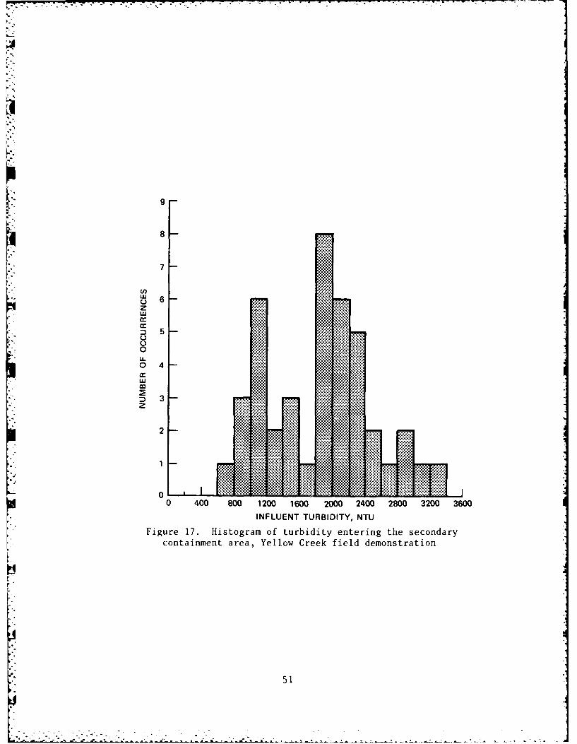
9
8
7
6,
z
D5
0
0 4
D 3 zX
2
*.*.**. *..*... ....* . . . . . .
... ... .... .
0 400 800 1200 1600 2000 2400 2800 3200 3600INFLUENT TURBIDITY, NTU
Figur 17.Histogram of turbidity entering the secondarycontainment area, Yellow Creek field demonstration
51
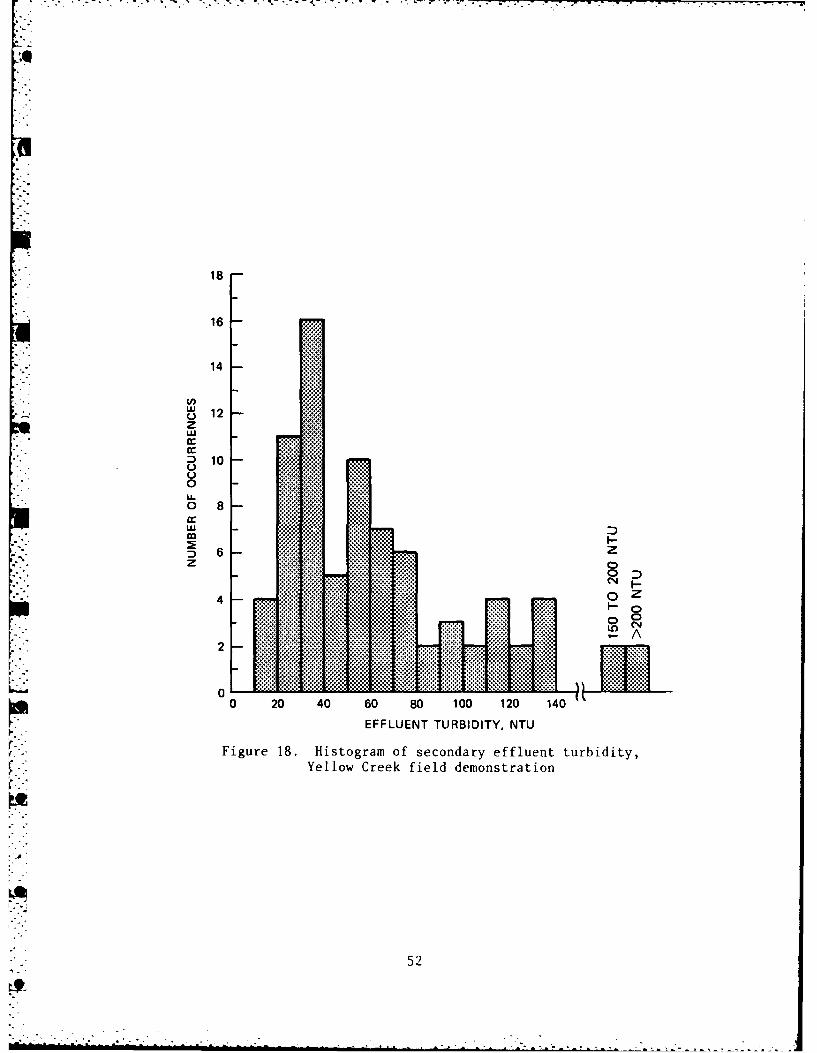
- ~ ~ - -V- -7r- - .
18
16
14
o 12z
fl 10
0 8IL
D 6zz0
4 oF-A0 0 4 0 80 100 120 140
F EFFLUENT TURBIDITY, NTU
r Figure 18. Histogram of secondary effluent turbidity,Yellow Creek field demonstration
52
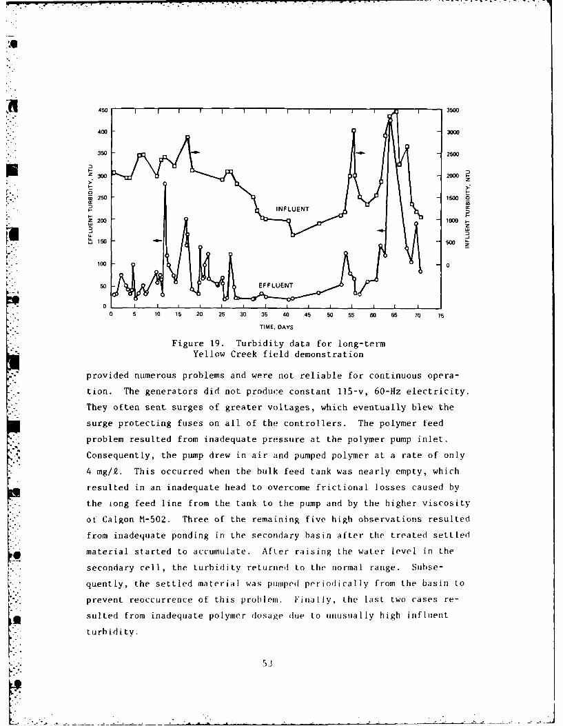
450 3500
400 3000
350 2500
z 300 - 2000 I
r.u -2 1500 0
- INFLUENT-
z 200 1000..
150 500
100 0
50 EFFLUENT
00 5 10 15 20 25 30 35 40 45 50 55 60 65 70 75
TIME, DAYS
Figure 19. Turbidity data for long-termYellow Creek field demonstration
provided numerous problems and were not reliable for continuous opera-
tion. The generators did not produce constant 115-v, 60-Hz electricity.
They often sent surges of greater voltages, which eventually blew the
surge protecting fuses on all of the controllers. The polymer feed
problem resulted from inadequate pressure at the polymer pump inlet.
Consequently, the pump drew in air and pumped polymer at a rate of only
4 mg/2. This occurred when the bulk feed tank was nearly empty, which
resulted in an inadequate head to overcome frictional losses caused by
the tong feed line from the tank to the pump and by the higher viscosity
ot Calgon M-502. Three of the remaining five high observations resulted
from inadequate ponding in the secondary basin after the treated settled
material started to accumulate. After raising the water level in the
secondary cell, the turbidity returned to the normal range. Subse-
quently, the settled material was pumped periodically from the basin to
prevent reoccurrence of this problem. Finally, the last two cases re-
suited from inadequate polymer dosage due to unusually high influent
turbidity.
53
I o. . . __J
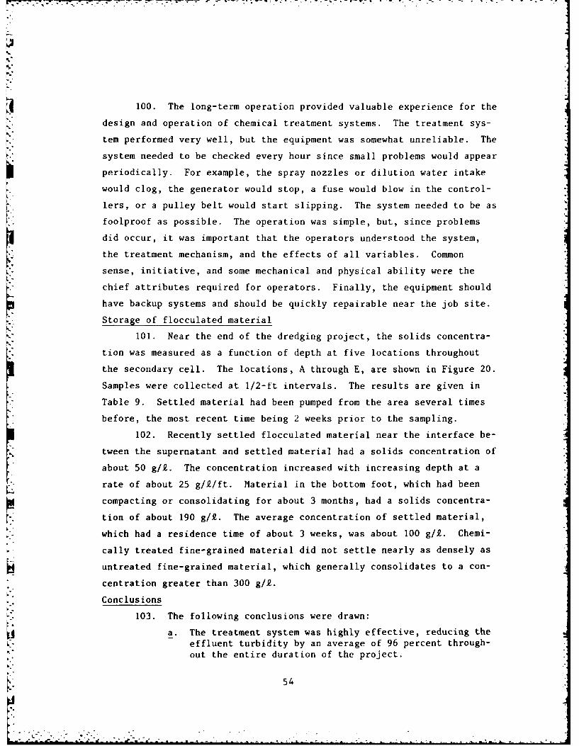
100. The long-term operation provided valuable experience for the
design and operation of chemical treatment systems. The treatment sys-
tem performed very well, but the equipment was somewhat unreliable. The
system needed to be checked every hour since small problems would appear
periodically. For example, the spray nozzles or dilution water intake
would clog, the generator would stop, a fuse would blow in the control-
lers, or a pulley belt would start slipping. The system needed to be as
foolproof as possible. The operation was simple, but, since problems
did occur, it was important that the operators understood the system,
the treatment mechanism, and the effects of all variables. Common
sense, initiative, and some mechanical and physical ability were the
chief attributes required for operators. Finally, the equipment should
have backup systems and should be quickly repairable near the job site.
Storage of flocculated material
101. Near the end of the dredging project, the solids concentra-
tion was measured as a function of depth at five locations throughout
the secondary cell. The locations, A through E, are shown in Figure 20.
Samples were collected at 1/2-ft intervals. The results are given in
Table 9. Settled material had been pumped from the area several times
before, the most recent time being 2 weeks prior to the sampling.
102. Recently settled flocculated material near the interface be-
tween the supernatant and settled material had a solids concentration of
about 50 g/.. The concentration increased with increasing depth at a
rate of about 25 g/9/ft. Material in the bottom foot, which had been
compacting or consolidating for about 3 months, had a solids concentra-
tion of about 190 g/9. The average concentration of settled material,
which had a residence time of about 3 weeks, was about 100 g/9. Chemi-
cally treated fine-grained material did not settle nearly as densely as
untreated fine-grained material, which generally consolidates to a con-
centration greater than 300 g/2.
4" Conclusions
103. The following conclusions were drawn:
a. The treatment system was highly effective, reducing theeffluent turbidity by an average of 96 percent through-out the entire duration of the project.
54
• [EFFLUENT
4i DISCHARGE
.N- ElE
D
d ee ttstMUD-... "PUMP
!:-- C
%" B
T:-RHEA TMENT,,:.::SYSTEM
SCALE
"'"0 50 100 FT
;-.'..Figure 20. Sampling locations in secondary containmenti::::i area, Yellow Creek field demo(ns tra tion
i':"'b. The required 10-mg/lk polymer feed dosage was higher than
deerind n helaboratory; but, at tesite, tecon-centration of fine-grained material to be treated wasgreater, less mixing was available, and better effluentquality was achieved.
c. The treatment system was capable of producing an effluentwith an average turbidity near 50 NTU under normaloperation.
d. The system performed best during continuous operation.
e. Improved treatment efficiency would have resulted if theweir structure had been designed to prevent leakage andto provide better mixing.
f. A reliable power supply must be acquired.
55
. The treatment operation required a capable, trained oper-ator to check the system regularly; to operate and main-tain the equipment; and to solve problems when theyappeared.
Costs of Chemical Treatment Demonstrations
104. The demonstrations provided information for estimating the
costs of future chemical treatment projects. Major costs were identi-
fied and quantified to the extent possible. Costs can be categorized as
engineering and design, nonexpendable equipment, construction, expend-
able supplies, operating labor, and repairs. Some of these costs are
independent of the prioject; others are a function of project duration
and/or volume to be dredged.
105. The first two demonstrations provided limited data due to
the brevity of the tests. Their costs are summarized in Table 10. The
total cost excluding nonexpendable equipment and construction costs was
about $80/hr or $0.25/yd3 of in situ material dredged for the first de-
monstration and about $55/hr or $0.14/yd3 for the second demonstration,
assuming that production was continuous and directly related to flow.
106. The long-term demonstration provided the best information on
costs. The costs are listed in Table 11. Excluding construction, the
cost averaged $0.20/yd3 or about $55/hr of production. The cost break-
down is given in Table 12. Labor and polymer costs were the main com-
ponents of the recorded costs for treatment, but the unknown construc-
tion costs might also be significant.
56
PART V: EVALUATION OF PIPELINE INJECTIONTREATMENT METHOD
107. Only preliminary laboratory and field studies have been per-
formed to evaluate the feasibility of injecting polymer into the dredge
pipeline to clarify dredged material slurries. Laboratory tests were
run on 100- and 120-g/2 slurries of settled dredged material from a con-
tainment area along the Yazoo River near Belzoni, Miss. The effects of
polymer addition on the settling rate of the material and on the solids
concentration of the supernatant were examined. The field study was
performed at the dredging site near Burnsville, Miss., described in
Part IV. The study examined the effects of polymer dosage, dredged ma-
terial variability, and injection location on the turbidity and solids
concentration reduction achieved during 10 min of settling. The studies
provided an estimate of the required polymer dosage but did not deter-
mine the ultimate effect of polymer injection at a given dosage on ef-
fluent quality from a containment area, ponding volume required for ef-
fective sedimentation, and storage requirements.
Laboratory Study
Background
108. Six 5-gal buckets of settled dredged material were collected
from an Upper Yazoo Project containment area near Belzoni, Miss. Two
buckets of coarse material were grabbed near the inlet of the basin and
four buckets of fine material were coliected near the weir. The fine-
grained material was classified as a silty clay (CL) with low plastic-
ity. The material was blended together to form mixtures of 50 percent
fine and 50 percent coarse material, 75 percent fine and 25 percent
coarse, and 100 percent fines. These mixtures were diluted with tap
water to produce the 100- and 120-g/k slurries used in the tests.
Test procedures
109. Six 1-k samples of each slurry were placed on a Phipps and
Bird multiple mixer. The samples were mixed at 100 rpm for I min to
57
ensure that the slurry was homogeneously suspended. Magnifloc 577C was
then added to the samples. The polymer dosages for the series were 0,
2, 4, 8, 16, and 32 mg/Q. Next, the 120-g/k slurries were mixed at
100 rpm for 10 sec and at 20 rpm for 5 min; the 100-g/ slurries were
mixed at about 150 rpm for 10 sec and at 50 rpm for 5 min. At this time
the samples were poured into I-k graduated cylinders and allowed to set-
tle. After the material started settling, the height of the interface
was read periodically to determine the settling rate. Also, samples
were collected at the midpoint of the supernatant to determine the sus-
pended solids removal. The mixing intensity used in these tests was too
low to be representative of conditions in a dredge pipeline.
Results
110. Jar tests on 2-g/k suspensions of the three mixtures indi-
cated that Magnifloc 577C was very effective. Dosages of 8, 6, and
4 mg/. performed best on suspensions of 100, 75, and 50 percent fines,
respectively. The dosage was directly proportional to the percent fines
in this concentration range.
111. The settling data for the three 120-g/k slurries are listed
in Table 13. The polymer dosages examined in this test did not affect
the settling rate of the slurries. At each time period the interface
height of each sample at the various dosages was very similar. The set-
tling rate and the concentration of the settled material decreased with
increasing concentration of fines in the slurries.
112. The solids concentration of the supernatant was measured
only for the slurry with 50 percent fines. The results are given in
Table 14. At each time period except the last, the supernatant concen-
tration was about the same at all polymer dosages examined. After
5-1/2 hr of settling, the solids concentration was reduced to 40 mg/k at
polymer dosages of 16 and 32 mg/i while at lower dosages the concentra-
tion was reduced to 280 mg/Q. This concentration was very low for fresh-
water clay sediments in the absence of polymer. The polymer at dosages
up to 32 mg/. did not significantly clarify the supernatant of 120-g/k
slurries.
113. The results of the settling tests on 100-g/Q slurries were
58
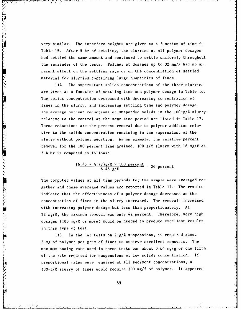
very similar. The interface heights are given as a function of time in
Table 15. After 5 hr of settling, the slurries at all polymer dosages
had settled the same amount and continued to settle uniformly throughout
the remainder of the tests. Polymer at dosages up to 32 mg/k had no ap-
parent effect on the settling rate or on the concentration of settled
material for slurries containing large quantities of fines.
114. The supernatant solids concentrations of the three slurries
are given as a function of settling time and polymer dosage in Table 16.
The solids concentration decreased with decreasing concentration of
fines in the slurry, and increasing settling time and polymer dosage.
The average percent reductions of suspended solids in the 100-g/Q slurry
relative to the control at the same time period are listed in Table 17.
These reductions are the percent removal due to polymer addition rela-
tive to the solids concentration remaining in the supernatant of the
slurry without polymer addition. As an example, the relative percent
removal for the 100 percent fine-grained, 100-g/2 slurry with 16 mg/f at
3.4 hr is computed as follows:
(6.45 - 4.77)g/f x 100 percent _ 26 percent6.45 g/f
The computed values at all time periods for the sample were averaged to-
gether and these averaged values are reported in Table 17. The results
indicate that the effectiveness of a polymer dosage decreased as the
concentration of fines in the slurry increased. The removals increased
with increasing polymer dosage but less than proportionately. At
32 mg/k, the maximum removal was only 42 percent. Therefore, very high
dosages (100 mg/f or more) would be needed to produce excellent results
in this type of test.
115. In the jar tests on 2-g/9, suspensions, it required about
3 mg of polymer per gram of fines to achieve excellent removals. The
maximum dosing rate used in these tests was about 0.64 mg/g or one fifth
of the rate required for suspensions of low solids concentration. If
proportional rates were required at all sediment concentrations, a
100-g/f slurry of fines would require 300 mg/f of polymer. It appeared
59
that the dosage requirement in terms of milligrams of polymer per gram
of material decreased with increasing slurry concentration but not
enough to keep the required polymer dosage low.
Conclusions
116. Polymer dosages up to 32 mg/k did not increase the settling
rate or density of freshly settled material. The polymer did slightly
enhance the clarity of the supernatant. The suspended solids concentra-
tion increased as the concentration of fines increased. The required
polymer dosage was related to the quantity of clay in the slurry. The
results of these experiments indicated that very high dosages would be
needed to treat slurries of fine-grained material. However, field con-
ditions would differ considerably from the conditions used in those
tests in that more mixing and longer settling time would be provided in
the field. Pipeline injection may be a viable alternative only for sed-
iments with a very small clay fraction.
Field Study
Background
117. The study was performed at a dredging site on the Tennessee-
Tombigbee Waterway near Burnsville, Miss. The location, dredging opera-
tion, and dredged material are described in detail in Part IV. The mate-
rial was 10 to 15 percent fine grained and contained only about 3 to
7 percent clays. The slurry concentration was about 200 g/Q. This ma-
terial was quite different from the material used in the laboratory
study described earlier. The flow rate was 16 cfs.
118. The purpose of the test was to determine the feasibility of
pipeline injection under typical field conditions. The effects of the
variability of the flow rate and influent solids concentration on the
effectiveness of a polymer dosage were examined. Polymer was injected
at two locations along the pipeline to investigate the effects of mixing
time on polymer effectiveness. The effects of polymer dosage on the re-
moval of suspended solids and turbidity were examined to determine likely
polymer dosage requirements for pipeline injection.
60
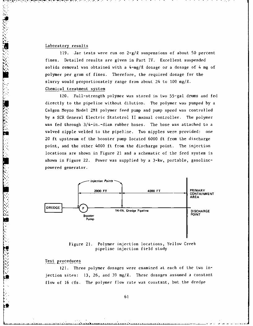
7 ....
Laboratory results
119. Jar tests were run on 2-g/.Q suspensions of about 50 percent
fines. Detailed results are given in Part IV. Excellent suspended
solids removal was obtained with a 4-mg/k dosage or a dosage of 4 mg of
polymer per gram of fines. Therefore, the required dosage for the
slurry would proportionately range from about 24 to 100 mg/k.
Chemical treatment system
120. Full-strength polymer was stored in two 55-gal drums and fed
directly to the pipeline without dilution. The polymer was pumped by a
Calgon Moyno Model 2M1 polymer feed pump and pump speed was controlled
by a SCR General Electric Statotrol II manual controller. The polymer
was fed through 3/4-in.-diam rubber hoses. The hose was attached to a
valved nipple welded to the pipeline. Two nipples were provided: one
20 ft upstream of the booster pump located 6000 ft from the discharge
point, and the other 4000 ft from the discharge point. The injection
locations are shown in Figure 21 and a schematic of the feed system is
shown in Figure 22. Power was supplied by a 3-kw, portable, gasoline-
powered generator.
Injection Points
20FT4000 FT PRIMARYCONTAINMENTAREA
14-IN. Dredge Pipeline DISCHARGE
Booster POINTPump
Figure 21. Polymer injection locations, Yellow Creekpipeline injection field study
Test procedures
121. Three polymer dosages were examined at each of the two in-
jection sites: 13, 26, and 39 mg/k. These dosages assumed a constant
flow of 16 cfs. The polymer flow rate was constant, but the dredge
61
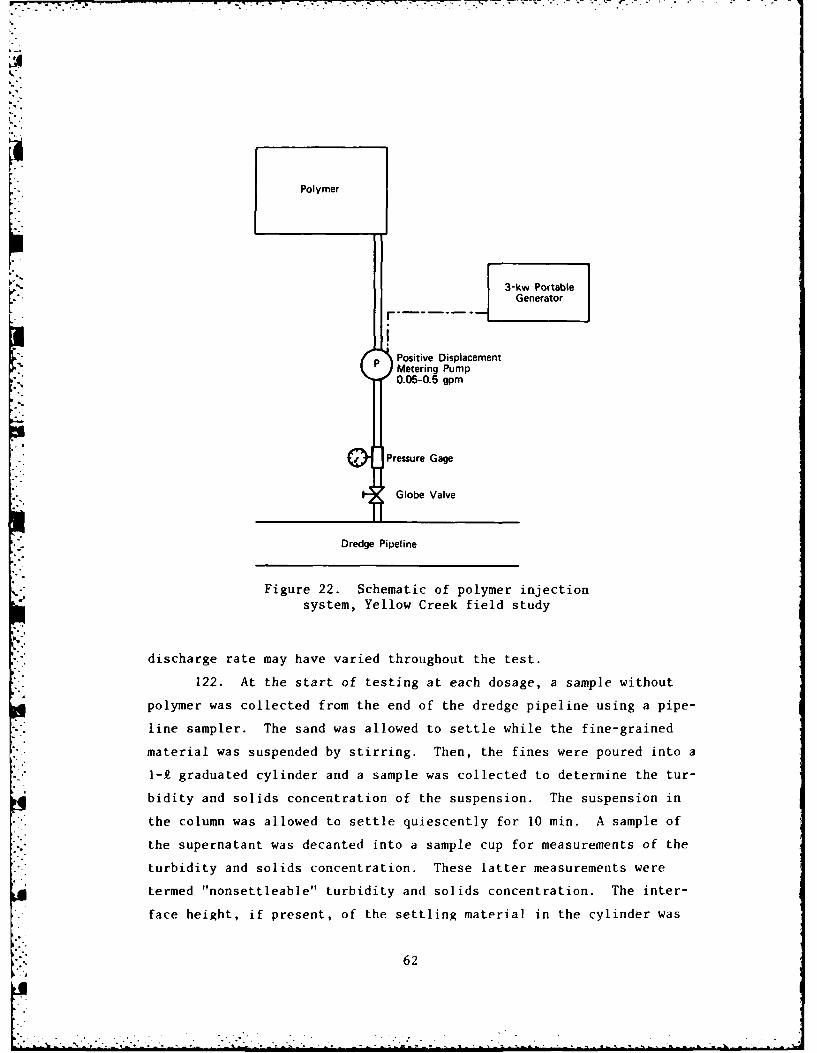
Polymer
3-kw PortableGenerator
Positive DisplacementMetering Pump0.05-0.5 gpm
, Pressure Gage
Globe Valve
Dredge Pipeline
Figure 22. Schematic of polymer injection
system, Yellow Creek field study
discharge rate may have varied throughout the test.
122. At the start of testing at each dosage, a sample without
polymer was collected from the end of the dredge pipeline using a pipe-
line sampler. The sand was allowed to settle while the fine-grained
material was suspended by stirring. Then, the fines were poured into a
1-k graduated cylinder and a sample was collected to determine the tur-
bidity and solids concentration of the suspension. The suspension in
the column was allowed to settle quiescently for 10 min. A sample of
the supernatant was decanted into a sample cup for measurements of the
turbidity and solids concentration. These latter measurements were
termed "nonsettleable" turbidity and solids concentration. The inter-
face height, if present, of the settling material in the cylinder was
62
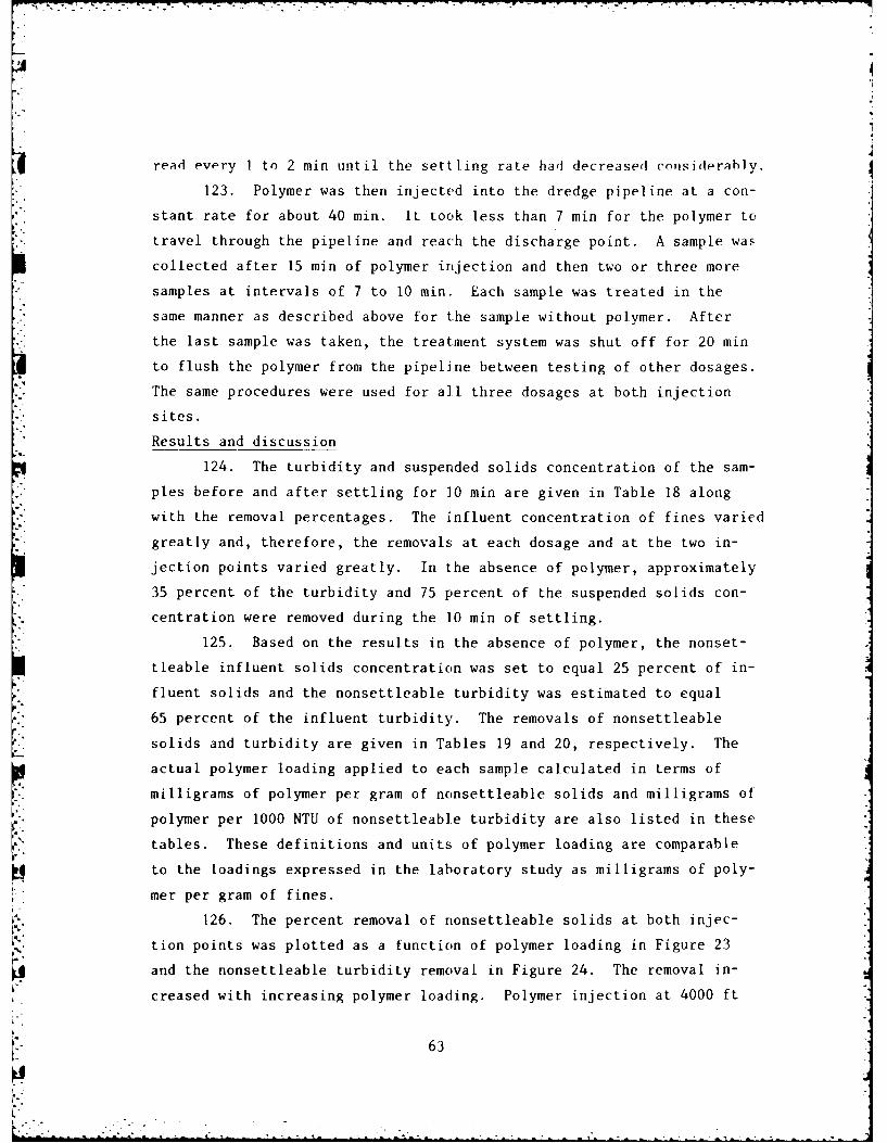
i4
read every I to 2 min until the settling rate had decreased considerably.
123. Polymer was then injected into the dredge pipeline at a con-
stant rate for about 40 min. It took less than 7 min for the polymer to
travel through the pipeline and reach the discharge point. A sample was
collected after 15 min of polymer injection and then two or three more
samples at intervals of 7 to 10 min. Each sample was treated in the
same manner as described above for the sample without polymer. After
the last sample was taken, the treatment system was shut off for 20 min
to flush the polymer from the pipeline between testing of other dosages.
The same procedures were used for all three dosages at both injection
sites.
Results and discussion
124. The turbidity and suspended solids concentration of the sam-
ples before and after settling for 10 min are given in Table 18 along
with the removal percentages. The influent concentration of fines varied
greatly and, therefore, the removals at each dosage and at the two in-
jection points varied greatly. In the absence of polymer, approximately
35 percent of the turbidity and 75 percent of the suspended solids con-
centration were removed during the 10 min of settling.
125. Based on the results in the absence of polymer, the nonset-
tleable influent solids concentration was set to equal 25 percent of in-
fluent solids and the nonsettleable turbidity was estimated to equal
65 percent of the influent turbidity. The removals of nonsettleable
solids and turbidity are given in Tables 19 and 20, respectively. The
actual polymer loading applied to each sample calculated in terms of
milligrams of polymer per gram of nonsettleable solids and milligrams ofpolymer per 1000 NTU of nonsettleable turbidity are also listed in these
tables. These definitions and units of polymer loading are comparable
to the loadings expressed in the laboratory study as milligrams of poly-
mer per gram of fines.
126. The percent removal of nonsettleable solids at both injec-
tion points was plotted as a function of polymer loading in Figure 23
and the nonsettleable turbidity removal in Figure 24. The removal in-
creased with increasing polymer loading. Polymer injection at 4000 ft
63
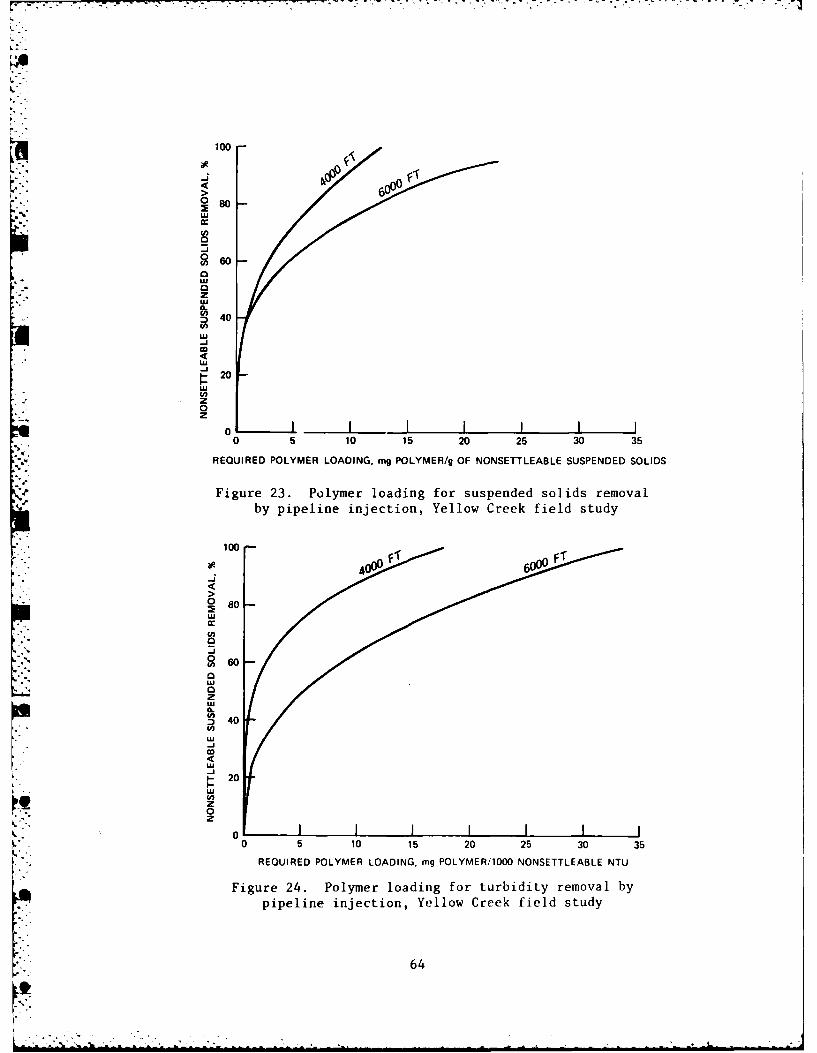
100
~80
0 8-J
~60
40
-J
~20w0
0 5 10 15 20 25 30 35
*REQUIRED POLYMER LOADING, mg POLYMER/g OF NONSETTLEABLE SUSPENDED SOLIDS
Figure 23. Polymer loading for suspended solids removalby pipeline injection, Yellow Creek field study
100 F
080
Cd,
-J
~60
40
-40
LU
-20.
02 0 5 1 0515 2 0 25 3 03 53
64
from the discharge point was more effective than injection before the
booster pump at 6000 ft from the discharge point. The mixing intensity
available in the pipeline corresponds to a mean velocity gradient G of900 sec The total mixing expressed in terms of nondimensional prod-
uct of mixing intensity and duration Gt was 240,000 at 4,000 ft and
360,000 at 6,000 ft. The optimal mixing for flocculation by polymer is
generally about 30,000, which corresponds to injection at 500 ft from
the discharge point. Better removals would be expected if the injection
location was optimized.
127. A comparison of polymer dosage requirements between the re-
- moval of turbidity and solids and between the two injection sites is
presented below. One milligram of polymer per 1000 nonsettleable NTU is
equivalent to about 0.8 mg of polymer per gram of nonsettleable solids.
At 4000 ft the removals of suspended solids and turbidity were equal at
a given dosage. At 6000 ft the remova. of solids was greater than the
turbidity removal at the same dosages. Under optimal mixing, the turbid-
ity and suspended solids removals would be similar to each other. The
required polymer dosage to achieve a given removal by injection at
4000 ft was about half as large as the dosage required for injection at
6000 ft.
Required Polymer LoadingNonsettleable at Injection Location
Solids Removal, % 4000 ft 6000 ft
60 2.8 4.6
80 6.8 12.4
100 12.7 26.3
Nonsettleable
Turbidity Removal,
60 2.0 8.6
80 6.8 18.5
100 17.7 33.4
128. The curves in Figures 23 and 24 showed that the increase in
removal decreased as the dosage increased. This type of diminishing
65
return is typical of flocculation by polymers and leads to high dosage
requirements for large removals. This can also be somewhat favorable
considering the variability of the influent because the removal percent-
ages would not decrease as much for an increase in the influent solids
and turbidity. The effects of this type of diminishing return decreased
with better mixing.
129. For this project, the required polymer dosage for excellent
removals with good mixing appeared to be about 4 mg of polymer per gram
of nonsettleable solids or 5 mg of polymer per 1000 NTU of nonsettleable
turbidity. This polymer loading rate is the same as required to treat
the effluent at the primary weir. In the field demonstration, the ef-
fluent averaged 1900 NTU and the required polymer dosage was 10 mg/i.
In terms of milligrams per litre, the required pipeline injection dosage
at the optimum location would have ranged from 8 to 50 mg/i due to the
variability of the influent. The dosage for average conditions would
have been 20 mg/f. If fed continuously at 20 mg/, the removal would
have ranged from nearly complete removal to about 70 percent. Of
course, the ultimate removal that would be realized at the primary weir
is unknown since pipeline injection has never been tested long enough to
determine its effect on containment area effluent quality.
130. The pipeline injection treatment system was simple and re-
quired little labor to maintain and operate since it had few components.
The most difficult part of the operation would be selecting the polymer
dosage. Immediate results can be seen at the discharge point but it
would take at least a day to determine the effects at the primary weir.
The effluent quality is particularly difficult to predict due to the
variability of the influent.
Conclusions
131. The following conclusions were drawn:
a. Full-strength liquid polymer was injected into thedredge pipeline and good removals were obtained at mod-erate dosages for this dredged material which had only avery small fraction of fines.
b. Better removals might have been observed if the injec-tion point was located closer to the discharge pointsince tile mixing was excessive.
66
c. The required polymer dosage was proportional to the con-centration of fines in the dredged slurry.
d. The required polymer loading rate in milligrams per gramor milligrams per 1000 NTU was the same as needed totreat effluents at the primary weir.
e. The dosage in milligrams per litre was considerablygreater for pipeline injection than for effluent treat-
., ment because the concentration of fines was larger inthe pipeline.
f. The effects of injecting polymer into the dredge pipelineon effluent quality, storage requirements, and contain-ment area design parameters for water quality are stilluntested and unknown.
F 67
.-.
PART VI: DESIGN AND OPERATING GUIDELINES FORTREATING DREDGED MATERIAL EFFLUENTS
132. This section of the report presents procedures and guidance
for designing and operating a chemical treatment system to clarify the
effluent from a dredged material containment area. Laboratory proce-
dures are presented to prepare representative suspensions, to select the
best polymer and dosage, and to evaluate the effects of mixing and vari-
able solids concentration on the effluent quality. Then, procedures are
given to design the polymer feed system including storage, dilution, and
injection; to design the weir and discharge culvert to provide adequate
mixing and minimize operating problems; and to design the secondary
basin to provide good settling and storage for treated material. Guid-
ance for operating the treatment system is given to maintain good per-
formance throughout the dredging project. These procedures are best
performed in conjunction with the design of the primary containment area
as presented in Engineer Manual (EM) 1110-2-5006 (Headquarters, Depart-
ment of the Army 1980), but these procedures may also be used for proj-
ects with existing or predesigned containment areas. A flowchart of
these procedures is shown in Figure 25.
Project Data
133. The following information should be obtained prior to per-
forming jar tests and designing the chemical treatment system:
a. Inflow rate based on past experience or on anticipateddredge size and a flow velocity of 15 fps. Largedredges may have higher velocities.
b. Effluent quality requirements based on legal constraints.
c. Salinity of water column determined by past experienceor laboratory tests.
d. Sediment grain-size analysis determined by laboratorytests.
e. Sediment plasticity (Atterberg limits) determined bylaboratory tests.
68
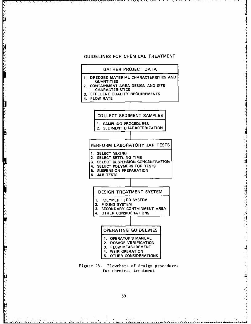
b7"
GUIDELINES FOR CHEMICAL TREATMENT
GATHER PROJECT DATA
1. DREDGED MATERIAL CHARACTERISTICS ANDQUANTITIES
2. CONTAINMENT AREA DESIGN AND SITECHARACTERISTICS
3. EFFLUENT QUALITY REQUIREMENTS4. FLOW RATE
COLLECT SEDIMENT SAMPLES
1. SAMPLING PROCEDURES2. SEDIMENT CHARACTERIZATION
PERFORM LABORATORY JAR TESTS
1. SELECT MIXING2. SELECT SETTLING TIME3. SELECT SUSPENSION CONCENTRATION4. SELECT POLYMERS FOR TESTS5. SUSPENSION PREPARATION6. JAR TESTS
DESIGN TREATMENT SYSTEM
1. POLYMER FEED SYSTEM2. MIXING SYSTEM3. SECONDARY CONTAINMENT AREA
,4. OTHER CONSIDERATIONS
OPERATING GUIDELINES
1. OPERATOR'S MANUAL2. DOSAGE VERIFICATION3. FLOW MEASUREMENT4. WEIR OPERATION5. OTHER CONSIDERATIONS
Figure 25. Flowchart. of design proceduresfor chemical treatment
69
f. Unified Soil Classification System classification ofsediment based on laboratory results of plasticity andgrain-size analyses.
". Primary and secondary containment area layouts anddesigns based on available sites.
h. Depths of containment areas and available difference inelevation between the two containment areas to be usedfor mixing.
i. Weir designs and effective weir length based on thedesigns.
j. Ponding depths based on designs and operation.
k. In situ volume to be dredged based on hydrographicsurveys.
1. In situ water content of sediment determined bylaboratory test.
m. Solids concentration of the dredged material slurrybased on past experience or assumed to be 145 g/.
Sediment Sampling and Characterization
Sediment sampling
134. The sediment samples used in the laboratory jar tests must
be representative of the material to be dredged in order to ensure the
validity of the laboratory results. The same samples used in the set-
tling tests for sizing the fine-grained dredged material containment
° •area may be used for the jar tests. Sampling should be performed in
accordance with the following recommendatioas from EM 1110-2-5006 (Head-
quarters, Department of the Army 1980):
a. Use a grab-type sampler capable of sampling upto a depth of about 12 in. Petersen or Shipeksamplers have been used satisfactorily.
b. Take sediment samples at a sufficient number oflocations to adequately define spatial varia-tions in the sediment character.
c. Collect at least 5 gal of sediment samples ateach sampling station.
70A'°
L
d. Collect samples in airtight and watertight con-tainers and place in a cold room (60 to 8°C)as soon after sampling as possible until organiccontent of samples can be determined. If or-ganic content is above 10 percent, the samplesshould remain in refrigeration until testingis completed.
Sediment characterization tests
135. The sediment properties affect the settling properties of
dredged material and, consequently, the solids concentration of the ef-
fluent to be treated at the primary weir. Therefore, the sediment must
be characterized before running laboratory tests on chemical treatment.
136. Salinity. The salinity of the sediment water and the bottom
water used to suspend and transport the dredged material must be mea-
sured or obtained from historical records. In estuarine environments,
the salinity may vary with depth, flow, wind, tidal cycle, and season.
Therefore, it is important to know the expected range of salinity during
the dredging project.
137. Salinity may be measured in two ways:
a. Conductivity. The salinity may be measured directly bya salinity-conductivity meter that electronically con-verts temperature-adjusted electrical conductivity into
salinity.
b. Dissolved solids or nonfiltrable residue. A detailedprocedure is presented in Standard Methods for the Exami-nation of Water and Wastewater (American Public HealthAssociation (APHA) 1976). Briefly,
(1) Filter water through a filter which has a pore sizeof I p or less.
(2) Pipette a known volume (about 25 ml) into a weigheddish and evaporate the sample 4 to 6 hr in a dryingoven at 103*-105*C.
(3) Cool the dish in a desiccator and then weighimmediately.
(4) Salinity (in parts per thousand) = mg residuem2 sample
138. Grain-size analysis. The grain-size distribution may vary
considerably at different locations. As the fraction of fines increases
71
in a freshwater sediment, the effluent solids concentration from the pri-
mary containment area would also increase, affecting the chemical treat-
ment requirements. Therefore, the test is important both for ensuring
that the sample is representative and for predicting the solids concen-
tration of the water to be treatLd. The procedures are given in Appen-
dix V of EM 1110-2-1906 (Headquarters, Department of the Army 1970).
139. Plasticity analyses. Plasticity analyses are necessary to
classify the fine-grained fraction using the Unified Soil Classification
System. The system is described in Technical Memorandum No. 3-357 pre-
pared at the U. S. Army Engineer Waterways Experiment Station (1953) and
the procedures for the analyses are described in EM 1110-2-1906 (Head-
quarters, Department of the Army 1970).
Solids concentration tests
140. The suspended solids concentration is the most frequently
measured parameter in the laboratory procedures. This measurement is
made during preparation of suspensions and evaluation of treatment ef-
fectiveness. There are three methods to measure suspended solids: total
solids, filtration, and centrifugation. Each is applicable under dif-
ferent circumstances. The total solids method measures both suspended
and dissolved solids. The dissolved solids concentration, if signifi-
cant, must be measured separately and subtracted from the total solids
concentration. The filtration method directly measures suspended solids.
The centrifugation method is a blend between the other two methods. It
attempts to measure suspended solids by measuring the total solids after
washing the dissolved solids out of a known volume of sample. The pro-
cedures outlined below are adapted from the methods given in EM 1110-2-
5006 (Headquarters, Department of the Army 1980).
141. Total solids method. This test is used when the suspended
* "solids concentration is large, compared to dissolved solids. It may be
used in other cases where the dissolved solids or salinity is known or
measured separately. To ensure accuracy, the test should generally be
used only for suspensions with a suspended solids concentration greater
than 1 g/k. These steps should be followed:
72
a. Obtain tared weight of a sample dish.
b. Thoroughly mix sample and pour into sample dish.
c. Weigh dish and sample and place in drying oven at 105 0Cuntil sample has dried to a constant weight (about 4 to6 hr).
d. Cool in desiccator and then weigh immediately.
e. Calculate suspended solids concentration C , in gramsper litre, as follows:
C =I'w. (Wt. S.S., g) x 1000 (1)c = [(Wt. S.S., g)/S.G. + (Wt. H20, g)]
where
Wt. S.S.= {(weight of dry sample and dish, g) - (weight ofdish, g) - [(Wt. H20 , g) x (S, ppt or g/)/1l000]}
S = salinity, ppt, or dissolved solids, g/.; if unknown infreshwater environments, use zero
S.G. = specific gravity of solids; use 2.67 if unknown
Wt. H20 [(weight of wet sample and dish, g) - (weight of drysample and dish, g)]
142. Filtration method. This method should be used for suspen-
sions having suspended solids concentrations of less than 1.0 g/. Any
quantitative filtering apparatus using a filter paper that has a pore
size of 1 p or less can be used for the test. The two most common set-
ups use either a Gooch crucible with a glass fibre filter paper or a
membrane filter apparatus. These steps should be followed:
a. Weigh filter.
b. Filter a measured volume of sample. The volume shouldbe sufficient to contain 5 mg of suspended solids.
c. Filter 10 ml of distilled water twice to wash out dis-solved solids.
d. Place filter in drying oven at 105°C until the samplehas dried to constant weight (usually 1 to 2 hr).
e. Cool in desiccator and weigh.
f. Calculate suspended solids concentration C , in gramsper litre, as follows:
C {[(weight of filter and dry solids, g)- (weight of filter, g)] x 1000
+ (volume of sample, ml)} (2)
73
u-.
- .. . " ° -
- • i.
-" - . . . • " " " ' .. . . . - ." " " .- -. -- - ." . . .. . . . .
143. Centrifugation method. This method is recommended for sam-
pies from saltwater environments that have a suspended solids concentra-
tion greater than 1 g/.e. It is particularly useful when the dissolved
solids concentration or salinity is unknown but expected to be signifi-
cant (greater than 10 percent of the suspended solids concentration).
This method is preferable to the total solids method when the dissolved
solids concentration is several or more times greater than the suspended
solids concentration. These steps should be followed:
a. Centrifuge a measured volume of sample until the liquidand solids have separated, yielding clear supernatant(several minutes should be sufficient).
b. Pour off supernatant being careful not to lose any ofthe solids.
c. Resuspend settled solids in distilled water by dilutingthe sample to its initial volume.
d. Repeat steps a through c twice to wash out all dissolvedsolids.
e. Pour sample into preweighed dish and then wash all re-maining solids in the centrifuge tube into the dishusing distilled water.
f. Place dish in drying oven at 105 0C until sample hasdried to constant weight (usually 4 to 6 hr).
s. Cool in desiccator and weigh.
h. Calculate suspended solids concentration C , in gramsper litre, as follows:
C = {[(weight of dish and dry solids, g)- (weight of dish, g)] x 1000
(volume of sample, ml)} (3)
Laboratory Jar Tests
General approach
144. Jar tests have been used to evaluate the effectiveness of
various aggregants under a variety of operating conditions for water
treatment. The procedures and evaluation process have been outlined by
Black et al. (1957) and Hudson (1981). However, conducting jar tests
and interpreting the results to determine design parameters are not sim-
pie tasks because there are many variables that can affect the tests.
74
Only experience can assist in applying the following jar test procedures
to a specific project. The reader is referred to a report by Jones,
Williams, and Moore (1978) for a discussion of equipment requirements
and the importance of flocculant type, flocculant concentration, floc-
culant addition methods, temperature, mixing and test equipment, and
intensity and duration of mixing on the jar test results.
145. Jar tests are used in these procedures to provide informa-
tion on the following design considerations:
a. Most effective flocculant.
b. Optimum dosage of flocculant.
c. Optimum feed concentration of flocculant.
d. Effects of dosage on removal efficiencies of turbidityand suspended solids.
e. Effects of concentration of influent suspension onremoval efficiencies.
f. Effects of mixing conditions on removal efficiencies.
.. Effects of settling time on removal efficiencies.
146. The general approach used in these procedures is as follows:
a. Using site-specific information on the sediment, dredgingoperation, containment areas, and effluent requirements--select mixing conditions, suspension concentration, set-tling time, and polymers for testing.
b. Prepare stock suspension of sediment.
c. Test a small number (four to six) of polymers that haveperformed well on similar dredged material. The testsshould be run on 2-g/k suspensions, which is a typicalconcentration for effluents from a well-designed contain-ment area for freshwater sediments containing clays. Ifgood removals are obtained at low dosages (10 mg/i orless), then select the most cost-effective polymer. Ifgood removals are not obtained, examine the polymer underimproved mixing and settling conditions and test the per-formance of other flocculants.
d. After selecting a polymer and its optimum dosage, examinethe effect of polymer feed concentration over the rangeof 1 to 30 g/k, typical concentrations used in the field,at the optimum dosage.
e. Determine dosage requirements for the expected range ofturbidity and suspended solids concentration to betreated at the primary weir.
75
f. Examine the effects of the range of possible mixing con-
ditions on the required dosage of flocculant for a typi-cal suspension.
&* Examine the effects of settling time on the removal ofsuspended solids and turbidity from a suspension of aver-age concentration using the selected dosage and likelymixing conditions.
147. The purpose of the approach described is to select an effec-
tive polymer for a suspension of a standard concentration, 2 g/k, which
is a typical effluent solids concentration. In this manner, the effec-
tiveness and dosage requirements of various polymers are easy to com-
pare. The other test variables are set to simulate anticipated field
conditions. After a polymer is selected, other variables are examined:
polymer feed concentration, solids concentration of suspension to be
treated, mixing, and settling time. The approach may be changed to fit
the needs and conditions of the specific study.
148. The details of each test typically are modified to satisfy
the constraints and conditions of the project and test. This procedure
generally requires judgment from experience with jar tests and chemical
treatment. The following procedures should be satisfactory in most
cases.
Selection of test conditions
149. Mixing intensity and duration. Prior to testing, the mix-
ing intensity and duration for the jar tests should be selected based on
project conditions. Assuming mechanical mixing will not be used in the
treatment system, the amount of mixing should be based on the available
head between the two containment areas, that is, the difference between
the water surfaces of the two areas which can be maintained throughout
the project (see Figure 26). The depth of the secondary area must be
sufficient to provide 2 to 3 ft of storage and 2 to 3 ft of ponding for
good settling. Preferably, 2 to 3 ft of head should be available for
mixing. The object is to convert the head into mixing energy in the
culvert(s) joining the two containment areas. The amount of head loss
is a function of flow rate, culvert diameter, and length. Table 21 pre-
sents typical mixing values Gt for good culvert mixing designs under a
76
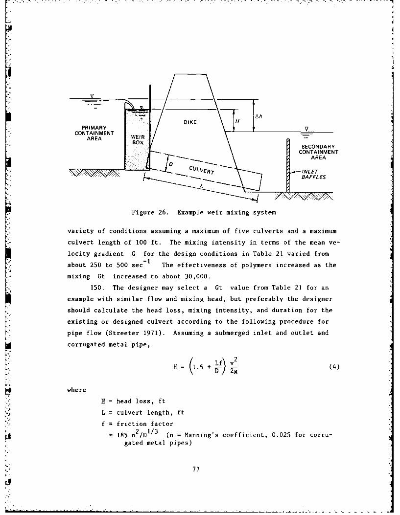
|V
AhDIKEH
PRIMARYCONTAINMENT
AREA WEIRBOX
SECONDARYCONTAINMENT
_ED AREA
BAFFLES
Figure 26. Example weir mixing system
variety of conditions assuming a maximum of five culverts and a maximum
culvert length of 100 ft. The mixing intensity in terms of the mean ve-
locity gradient G for the design conditions in Table 21 varied from-I
about 250 to 500 sec The effectiveness of polymers increased as the
mixing Gt increased to about 30,000.
150. The designer may select a Gt value from Table 21 for an
example with similar flow and mixing head, but preferably the designer
should calculate the head loss, mixing intensity, and duration for the
existing or designed culvert according to the following procedure for
pipe flow (Streeter 1971). Assuming a submerged inlet and outlet and
corrugated metal pipe,
L2 H = 1 . + v__v
2g (4)
where
H = head loss, ft
L = culvert length, ft
f = friction factor
= 185 n2/D 1/ (n = Manning's coefficient, 0.025 for corru-gated metal pipes)
77
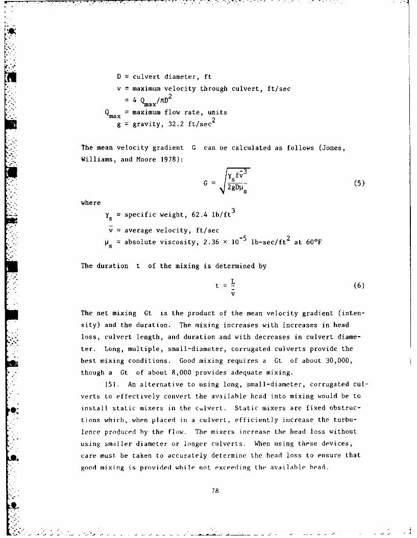
D = culvert diameter, ft
v maximum velocity through culvert, ft/sec
4 Q mnD2max
Q = maximum flow rate, unitsmax2
g = gravity, 32.2 ft/sec2
"*. The mean velocity gradient G can be calculated as follows (Jones,
" Williams, and Moore 1978):
yfvG = p5s
where
Ys specific weight, 62.4 lb/ft
v = average velocity, ft/sec
Ps= absolute viscosity, 2.36 x 10⁻⁵ at 60F
The duration t of the mixing is determined by
t =L (6)v
The net mixing Gt is the product of the mean velocity gradient (inten-
sity) and the duration. The mixing increases with increases in head
loss, culvert length, and duration and with decreases in culvert diame-
ter. Long, multiple, small-diameter, corrugated culverts provide the
best mixing conditions. Good mixing requires a Gt of about 30,000,
.- though a Gt of about 8,000 provides adequate mixing.
151. An alternative to using long, small-diameter, corrugated cut-
verts to effectively convert the available head into mixing would be to
install static mixers in the culvert. Static mixers are fixed obstruc-
tions which, when placed in a culvert, efficiently increase the turbu-
lence produced by the flow. The mixers increase the head loss without
using smaller diameter or longer culverts. When using these devices,
care must be taken to accurately determine the head loss to ensure that
good mixing is provided while not exceeding the available head.
78
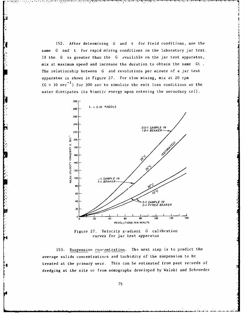
15 2 . After determining G and t for field conditions, use the
same G and t for rapid mixing conditions in the laboratory jar test.
If the G is greater than the G available on the jar test apparatus,
mix at maximum speed and increase the duration to obtain the same Gt
The relationship between G and revolutions per minute of a jar test
apparatus is shown in Figure 27. For slow mixing, mix at 20 rpm
(G = 10 sec 1) for 300 sec to simulate the exit loss conditions as the
water dissipates its kinetic energy upon entering the secondary cell.
300-
280 - 1- x 3-IN. PADDLE
260 -
240 -
0.5-Q SAMPLE IN
220- 1.0-V BEAKER
w200i
i18 -
160 oC,
>140
"..-J 120
zL Z~ 100 - -10 •- SAMPI E IN
I-Q BEAKER--
80 -oC /d C60-
40 - - 2-12 SAMPLE .IN.. .
0 20 40 60 80 100 120 140
REVOLUTIONS PER MINUTE
Figure 27. Velocity gt-adient G calibrationcurves for jar test apparatus
153. Suspension concentration. The next step is to predict the
average solids concentratiils and turbidity of the suspension to be
treated at the primary weir. This can be estimated from past records of
dredging at the site or from nomographs developed by Walski and Schroeder
79
(1978). Two nomographs were developed: one for freshwater clays that
undergo flocculent settling, and the other for freshwater silts and
saltwater sediments that undergo zone settling. The nomographs relate
the flow rate, effective weir length, and ponding depth (depth of water
above interface of settled material at the weir) to the suspended solids
concentration of water discharged over the weir. These relationships
are considered valid for well-designed primary containment areas that
are properly sized for the efficient retention of suspended solids by
gravity sedimentation. Procedures for containment area design consider-
ing both flocculent and zone settling are found in EM 1110-2-5006 (Head-
quarters, Department of the Army 1980). The nomographs are shown in
Figures 28 and 29.
154. Selection of which nomograph to use is based on the salinity
and soil classification. If the material is a silt (either ML, MH, or
OL), use Figure 28. If the material is a clay (either CL, CH, or OH),
it is necessary to determine the salinity of the suspending water. If
the salinity is greater than 3 ppt, the sediment should be considered to
- ."be from a saltwater environment and Figure 28 should be used. If the
salinity is less than 1 ppt, the clay will settle as a freshwater clay
and Figure 29 should be used. For salinities between 1 and 3 ppt, the
settling properties of a 100-g/ slurry of sediment in natural water
should be examined to determine whether it displays zone settling or
flocculent settling. For zone settling, use Figure 28, and use Fig-
ure 29 for flocculent settling.
155. To use the nomographs, draw a horizontal line at the design
flow rate. At the point where it intersects with the effective weir
length of the design, draw a vertical line down to the ponding depth to
be maintained at the weir. Then, draw a horizontal line from the point
* of intersection to the left vertical axis and read the suspended solids
concentration in grams per litre. This concentration is an estimate of
the average suspension concentration.
156. Settling time for flocculated material. The next variable
to establish is settling time. Flocculated (chemically treated) mate-
rial settles at a rate of about 0.25 ft/min (Jones, Williams, and Moore
80
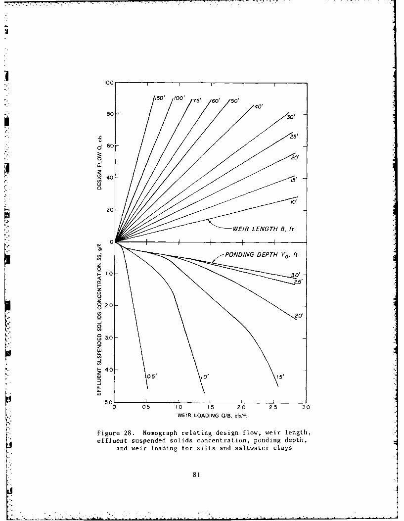
00
/5'10'75' 60' 50'40'
80- 30'
60
20-
00
20-
z
0
NzC)0 -U
z
WEIR LoDN 0/t5/sf
810 :110 05 1 15 2 25 I
WEI LOA IN ,.4.t c.A..L
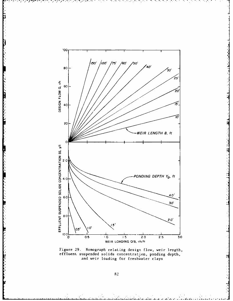
150' /00' 75' 0'1 50so- 40' 30'
25'
60-
0-iU-
00
0
0 2
LU040LU
0
4-0-
U-
LU
WERLAIG /ncsfFiue2.0mgahrltn einfowi eghefletsseddooiscnetaiopnigdph
an erlaigfrfehae ly
-82
U. 0~ 1.0,.. .- -
1978). The required ponding depth for good settling is about 2 to 3 ft;
therefore, a minimum of 10 min is needed for settling. Also, due to
basin inefficiencies, some of the water will reach the secondary weir in
10 to 20 percent of the theoretical detention time. For secondary con-
tainment areas, this may be as short as 10 to 20 min, though the mean
detention time may be about 50 min. Based on this information, the set-
tling time in the jar test should be set at 10 min. The effect of set-
tling time on suspended solids removal can be evaluated in the jar test
procedures.
157. Selection of polymers for testing. The final consideration
before starting the jar tests is the selection of polymers to be tested.
To simplify the operation of feeding and dispersing the polymer at the
project, a low viscosity liquid polymer should be used. Some polymers
effective on dredged material are given in Part III. Polymer manufac-
turers may be able to suggest others. The manufacturers can also recom-
mend maximum polymer feed concentrations.
158. Polymers selected for testing should be nontoxic, nonhazard-
ous, and unreactive. Polymer manufacturers can provide detailed infor-
mation on the environmental properties of their products. Also, the
U.S. Environmental Protection Agency has approved many polymers for use
on potable water at the desired dosages. Very little of an applied dos-
age is expected to be discharged from the containment area since the
polymer adsorbs on the solids and settles in the containment area.
Therefore, polymers should not be detrimental to the quality of the re-
ceiving waters. Furthermore, Wang and Chen (1977) showed that polymers
did not increase the long-term release of contaminants or nutrients from
treated dredged material. Consequently, there appears to be no reason
to consider polymer-treated, uncontaminated dredged material as a hazard-
ous substance requiring special considerations.
Suspension preparation
159. Dredged material tha3t is discharged over the weir is com-
posed of only the finest fraction of the sediment. In many cases, this
material has been suspended and mixed in the primary containment area
for several days while the coarser material settled. Therefore, to
83
Of
obtain representative suspensions for testing, the following procedure
is recommended:
a. Thoroughly mix sediment sample to ensure homogeneity.Then, blend together equal portions of each sample toform a representative composite of the sediment. Grain-size analysis and soil classification may be performedon this material to characterize the mixture and to com-pare it with previous characterizitions of the sediment.
b. If the sediment mixture contains more than 10 percent(dry weight basis) coarse grained (>No. 200 sieve) mate-rial, the material should be sieved through a standardU. S. series No. 200 sieve. The fines can be washedthrough the sieve using water from the bottom of thewater column at the dredging site. If this water is un-available, tap water may be used in its place, but thesalinity of the suspension of fines (<No. 200 sieve)must be adjusted to naturally occurring salinity of thebottom waters at the project site.
c. Prepare a supply of 2.0-g/2 suspensions by diluting awell-mixed portion of the slurry of fines with waterfrom the dredging site or with tap water adjusted withsalt to the same salinity. Suspensions at other concen-trations would be prepared in the same manner.
Jar test procedures
*160. Having established the test variables, the designer is ready
to start the laboratory jar test procedures. Care must be exercised in
the tests to ensure that each sample is handled uniformly. The tests
must be performed in a standard manner to evaluate the results. The
following variables must be controlled:
a. Identical test equipment and setup.
b. Suspension preparation.
c. Sample temperature.
d. Polymer feed concentration and age.
e. Polymer dosage.
f. Sample premix time and intensity.
-. Polymer addition method.
h. Duration and intensity of rapid mixing.
i. Duration and intensity of slow mixing.
,j. Settling time.
84
k. Sampling method.
1. Laboratory analyses of samples.
161. All of the following procedures described in this section
are not necessary for every project. The required tests are dependent
on the purpose of the study, and some tests can be eliminated based on
past experience of treating dredged material under similar circumstances.
162. Selection of polymer. The laboratory jar test procedures
are as follows:
a. Fill a 1- or 2-2 beaker with a 2.0-g/ suspension offine-grained dredged material.
b. Mix at 100 rpm and incrementally add polymer at a dosingof 2 mg/2 until flocs appear. Note total dosage applied.(Use a polymer feed concentration of 2 g/2 or 2 mg/ml.)
c. Fill six 1- or 2-9 beakers with a 2.0-g/2 suspension ofdredged material and measure the suspended solids con-centration and turbidity of the suspension.
d. Mix at 100 rpm for 1 min and then rapidly add the desiredpolymer dosage to each beaker. Use a range of polymerdosages from 0 mg/2 to about twice the dosage determinedin step b.
e. Immediately adjust the mixing to the desired G forrapid mixing as determined earlier. Mix for the desiredduration t also determined earlier.
-1f. Reduce the mixer speed to a G of 10 sec and slow mix
for 300 sec.
". Turn off mixer and let settle for 10 min.
h. Withdraw samples from the 700-ml level of 1-2 beakersand from the 1400-ml level of 2-9 beakers.
i. Measure the suspended solids concentration and turbidityof the samples. The test data should be recorded on areport form similar to the one shown in Figure 30. Alsorecord any significant observations such as nature, size,and settling characteristics of the floes; time of flocformation; and any peculiarities.
j. Repeat steps c through i as needed to adequately definethe effects of dosage on clarification.
k. Repeat steps a through I for the other polymers. A dos-age of 10 mg/2 should reduce the solids concentrationsby 95 percent if the polymer is effective. Examineenough polymers to find at least two effective polymers.
85
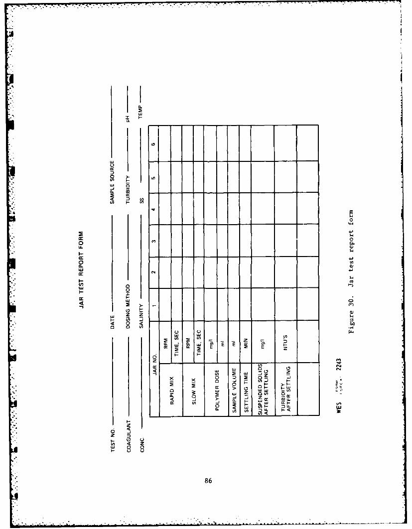
a.
wL
CDi:
V) i
LU 0
4 4
U )- 4 .)U
0 4
LL 0
c4-4
00
o U0.0
LaF1-
((U)~L __ _
a- C
E 2z
4 0 0
LU LU-) z j _
U) c U n
0 0)- c-
<. w ~ U 0
W) U) LL. <
o 4,4
z D
LU 0 0L-C) C.
86
• . ._ - • - . , * - . - . . . . . . - . / - .
1. Select the most cost-effective polymer that can be easilyfed and dispersed.
163. Selection of polymer feed concentration. After selecting the
best polymer, the effects of polymer feed concentration and polymer solu-
tion age on the removals can be evaluated. Some polymers require large
dilution factors and aging following dilution to maximize their effec-
tiveness. This test is not required if adequate dilution water and solu-
tion aging are provided in the design to meet the manufacturer's recom-
mendations. Often, to simplify the treatment system design, these recom-
mendations are not met. The test is performed as follows:
a. Prepare six fresh solutions of the selected polymerranging in concentration from about 1 to 40 g/P.
b. Fill six beakers as in step c of paragraph 162.
c. M~x at 100 rpm for I min and then rapidly add thepolymer solutions at the effective dosage establishedearlier and in the same manner.
d. Continue to follow the procedures outlined in steps ethrough i of paragr;iph 162.
e. Allow two solutions to age as desired (between 1 hrand I day) and repeat steps b through d.
164. Determination of required dosage. The dosage requirements
of the selected polymer for the anticipated average solids concentra-
tion of the primary effluent suspension to be treated at the primary
weir should be evaluated. This concentration was determined pre-
viously f:an past records or from the nomographs in Figures 28 and 29.
The procedure is as follows:
a. Fill six beakers with suspensions at the desiredconcentration of the fine-grained fraction of dredgedmaterial. Measure the suspended solids concentrationand turbidity of the suspension.
b. Mix at 100 rpm for I min and then rapidly add thedesired polymer dosage to each beaker. The range ofdosages should be proportional to the solids concen-tration.
c. Continue to follow the procedures outlined in steps ethrough j of paragraph 162.
87
L.
Other suspensions with different solids concentrations may be examined
in the same manner to determine the possible range of dosages required
for the project and the possible range of effluent quality obtainable
under conditions of variable primary effluent solids concentration to
be treated.
165. Effects of mixing. Other mixing conditions can be examined
to determine the impact of low flow conditions and to evaluate whether
the mixing is adequate. The effects of increasing the mixing by a Gt
of 5,000 and 10,000 and of decreasing the flow rate by 50, 75, and 90
percent on the polymer dosage requirements can be evaluated as follows:
a. Calculate the new mixing intensity and duration.
b. Fill six beakers with a suspension at the anticipatedaverage solids concentration.
c. Mix at 100 rpm for 1 min and then rapidly add thedesired polymer dosage to each beaker. Select a rangeof dosages surrounding the optimum dosage determinedin the last set of experiments on the same suspension.
d. Immediately adjust the mixing to the G value calcu-lated in step a for rapid mixing and mix for the cal-culated duration t
e. Follow the procedures outlined in steps f through iof paragraph 162.
166. Effects of settling time. The effects of settling time on
effluent quality can be examined as follows:
a. Determine the range of settling time of interest bearingin mind that the secondary basin will be hydraulicallyinefficient and the settling conditions are not quiescent.
b. Follow procedures outlined in steps c through i of para-graph 162 but adjust the settling time and samplingschedule to cover the range determined above.
Design of Chemical Treatment Systems
167. This section presents the design procedures for chemical
clarification of primary containment area effluents. The design is com-
posed of three subsystems: (a) the polymer feed system including stor-
age, dilution, and injection; (b) the weir and discharge culvert for
88
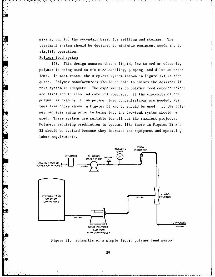
- .' 2. - . -' J " " - . -
. ",' -'- - ".
"-
- -w . '- .. .- ' ' " "--"" -- "-'- "
. ... . " "
mixing; and (c) the secondary basin for settling and storage. The
treatment system should be designed to minimize equipment needs and to
simplify operation.
Polymer feed system
168. This design assumes that a liquid, low to medium viscosity
polymer is being used to minimize handling, pumping, and dilution prob-
lems. In most cases, the simplest system (shown in Figure 31) is ade-
quate. Polymer manufacturers should be able to inform the designer if
this system is adequate. The experiments on polymer feed concentrations
and aging should also indicate its adequacy. If the viscosity of the
polymer is high or if low polymer feed concentrations are needed, sys-
tems like those shown in Figures 32 and 33 should be used. If the poly-
mer requires aging prior to being fed, the two-tank system should be
used. These systems are suitable for all but the smallest projects.
Polymers requiring predilution in systems like those in Figures 32 and
33 should be avoided because they increase the equipment and operating
labor requirements.
"-'. F LOW•PRESSURE FO
PRSGAGE INDICATOR
STAIE ADLTION VALVE
DILUTION WATERSUPPLY OR INTAKE
MIXINGS TO0RA GE TAN K E DUCTOROR DRUM
CONTAINERS
TO PROCESS
CONC. POLYMERFEED PUMP
WITH CONTROLLER
Figure 31. Schematic of a simple liquid polymer feed system
89
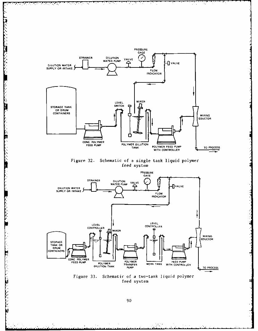
PRESSUREGAGE ________
STRAINER DILUTION VALVEWATER PUMP
=". VALVE
DnLUTION WATERSUPPLY OR INTAKE L
F LOW
INDICATOR
STORAGE TANK SWITCH
CONTAINERS MIXING
EDUCTOR
CONC. POLYMERFEED PUMP POLYMER DILUTION
TANK POLYMER FEED PUMP TO PROCESSWITH CONTROLLER
Figure 32. Schematic of a single tank liquid polymerfeed system
PRESSUREGAGE________-
STRAINER DILUTION VALVEWATER PMSVALVE
DILUTION WATER
SUPPLY OR INTAKEFLOW
INDICATOR
LEVEL LEVEL
CONTROLLER CONTROLLER
MIXER
EDUCTORSTORAGE
TANK OR UtDRUM
• LCONTAINE RS
CONC. POLYMERFEED PUMP POLYMER POLYMER WRTAK FEED PUMP
TRANSFER WORK TANK WITH CONTROLLERDILUTION TANK PUMP TO PROCESS
Figure 33. Schematic of a two-tank liquid polymerfeed system
90
169. Storage. The polymer can be stored at the site in the de-
livery containers, either 55-gal drums or bulk shipping tanks. The
polymer can be fed directly from these containers or transferred to a
polymer feed tank. Provisions should be made to guard against freezing.
The feed tank may need to be heated or stored in a heated shelter to
lower the viscosity and facilitate pumping on cold days. The size of
the feed tank and storage facilities is dependent on the project.
- 170. The volume of polymer required for the project may be calcu-
lated as follows:
Total Volume of Inflow, 23
= (Volume to be dredged, yd x (In situ Sediment Conc., g/2)
x 764.4 2/yd3 (Dredged Material Slurry Conc., g/2) (7)
Total Volume of Settled Material, k, (Total Volume of Inflow, x) x (Influent Slurry Conc., g/2)
(Conc. of Settled Material, g/2) (8)
If the concentration of settled material is unknown, it is generally
conservative to let
Total Volume of Settled Material, 2
" 2 x (Volume to be dredged, yd 3) x 764.4 k/yd 3 (9)
Then,
Total Volume to be Treated, k = (Total Volume of Inflow, k)- (Total Volume of Settled Material, k) (10)
Total Volume of Polymer Required, gal= (Required Dosage, mg/k) x (Total Volume to be Treated, 2)
(Specific Weight of Polymer, kg/k)
± 106 mg/kg 3.785 k/gal (11)
Total Poundage of Polymer, lb
= (Total Volume of Polymer, gal) x 3.785 2/galx (Specific Weight of Polymer, kg/k) x 2.205 lb/kg (12)
91
171. Polymer pumping. Concentrated polymer solutions should be
fed using a positive displacement pump. The pump speed should be regu-
lated by either a manual or automatic controller. The pump should be
capable of discharging a wide range of flows to handle the possible range
of required polymer dosages and flow rates of water to be treated. The
pump capacity should be at least twice the maximum anticipated polymer
feed rate or four times the average feed rate. The minimum pumping rate
must be less than 10 percent of the average anticipated polymer feed
rate to handle low flow conditions.
172. The average polymer feed rate is
Avg. Feed Rate, ml/sec
(Avg. Flow Rate, cfs) X (Avg. Required Dosage, mg/k)
x 28.31 k/ft3 (Specific Weight of Polymer, g/ml)
1000 mg/g (13)
173. The polymer pump flow capabilities should range from about
Pump Range, ml/sec = (0.1 to 4) x (Avg. Feed Rate, ml/sec) (14)
Two polymer pumps operated in paralLel may be required to provide the
desired range of feed rates.
174. If the polymer requires a tan for predilution as in Fig-
ures 32 and 33, the polymer should be diluted by a factor of 10 or 20
in the tank. The polymer feed rate would then increase by this same
factor.
175. Polymer tanks. The polymer feed tanks and dilution tanks
should be large enough to feed polymer for I to 2 days under average
conditions. The average daily concentrated polymer feed volume is
Daily Volume, gal/day (Avg. Feed Rate, mi/sec)x 86,400 sec/day 3,78.5 ml/gal (15)
176. Polymer dilution. The polymer must be diluted to aid feeding
92
D-T134 73 R CHEMICAL CLRIFICRTION METHODS FOR CONFINED DREDGED 2/2MATERIAL DISPOSAL(U) ARMY ENGINEER WATERWAYS EXPERIMENTSTATION VICKSBURG MS P R SCHROEDER JUL 83UNCLASSIFIED WES-TR-D-83-2 F/G 13/2 NLE=hlEEllEEEll
EIIIIIIIIIIIEEEIIIEIIIIIIIEEElIIIIII
*. '-..
"
I-,
.9
k
1.0 um SAW5- %-.
LI M2
IV
MICROCOPY RESOLUTION TEST CHART
NATIONAL BUREAU
OF STANDARDS-1963 A
07.
-.. ]
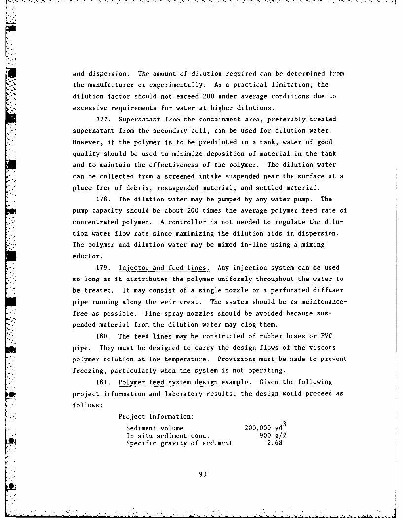
i -.. . . v : .. . - . ,. -. ., ..: .: .7 - -.. .: . - - - - - : ... . .
and dispersion. The amount of dilution required can be determined from
the manufacturer or experimentally. As a practical limitation, the
dilution factor should not exceed 200 under average conditions due to
excessive requirements for water at higher dilutions.
177. Supernatant from the containment area, preferably treated
supernatant from the secondary cell, can be used for dilution water.
However, if the polymer is to be prediluted in a tank, water of good
quality should be used to minimize deposition of material in the tank
and to maintain the effectiveness of the polymer. The dilution water
can be collected from a screened intake suspended near the surface at a
place free of debris, resuspended material, and settled material.
178. The dilution water may be pumped by any water pump. The
pump capacity should be about 200 times the average polymer feed rate of
concentrated polymer. A controller is not needed to regulate the dilu-
tion water flow rate since maximizing the dilution aids in dispersion.
The polymer and dilution water may be mixed in-line using a mixing
eductor.
179. Injector and feed lines. Any injection system can be used
so long as it distributes the polymer uniformly throughout the water to
be treated. It may consist of a single nozzle or a perforated diffuser
pipe running along the weir crest. The system should be as maintenance-
free as possible. Fine spray nozzles should be avoided because sus-
pended material from the dilution water may clog them.
180. The feed lines may be constructed of rubber hoses or PVC
pipe. They must be designed to carry the design flows of the viscous
polymer solution at low temperature. Provisions must be made to prevent
freezing, particularly when the system is not operating.
181. Polymer feed system design example. Given the following
project information and laboratory results, the design would proceed as
follows:
Project Information:
Sediment volume 200,000 yd3
In situ sediment conc. 900 g/QSpecific gravity of ;d(Jiment 2.68
93
•. , .-.. . . .
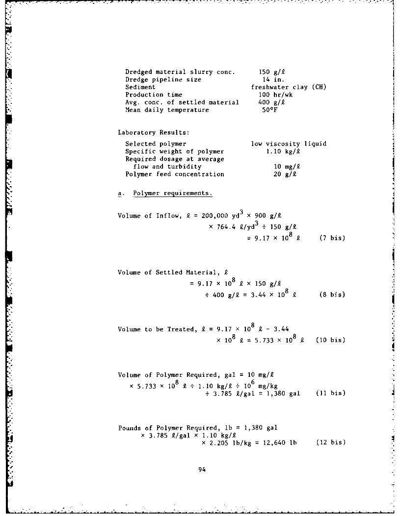
Dredged material slurry conc. 150 g/i
Dredge pipeline size 14 in.Sediment freshwater clay (CH)
Production time 100 hr/wkAvg. conc. of settled material 400 g/i
Mean daily temperature 50OF
Laboratory Results:
Selected polymer low viscosity liquid
Specific weight of polymer 1.10 kg/iRequired dosage at average
flow and turbidity 10 mg/iPolymer feed concentration 20 g/i
a. Polymer requirements.
3Volume of Inflow, i = 200,000 yd3 X 900 g/£
x 764.4 k/yd3 + 150 g/i
= 9.17 x 10⁸ £ (7 bis)
Volume of Settled Material, £
9.17 x 108 k x 150 g/£
400 g/i = 3.44 x 10⁸ £ (8 bis)
Volume to be Treated, £ = 9.17 x 10⁸ £ - 3.44
x 108 £ = 5.733 x 10⁸ £ (10 bis)I I
Volume of Polymer Required, gal = 10 mg/i
x 5.733 x 10⁸ 1.10 kg/ 10 6 mg/kg
3.785 i/gal = 1,380 gal (11 bis)
Pounds of Polymer Required, lb = 1,380 galx 3.785 i/gal x 1.10 kg/k
x 2.205 lb/kg = 12,640 lb (12 bis)
94
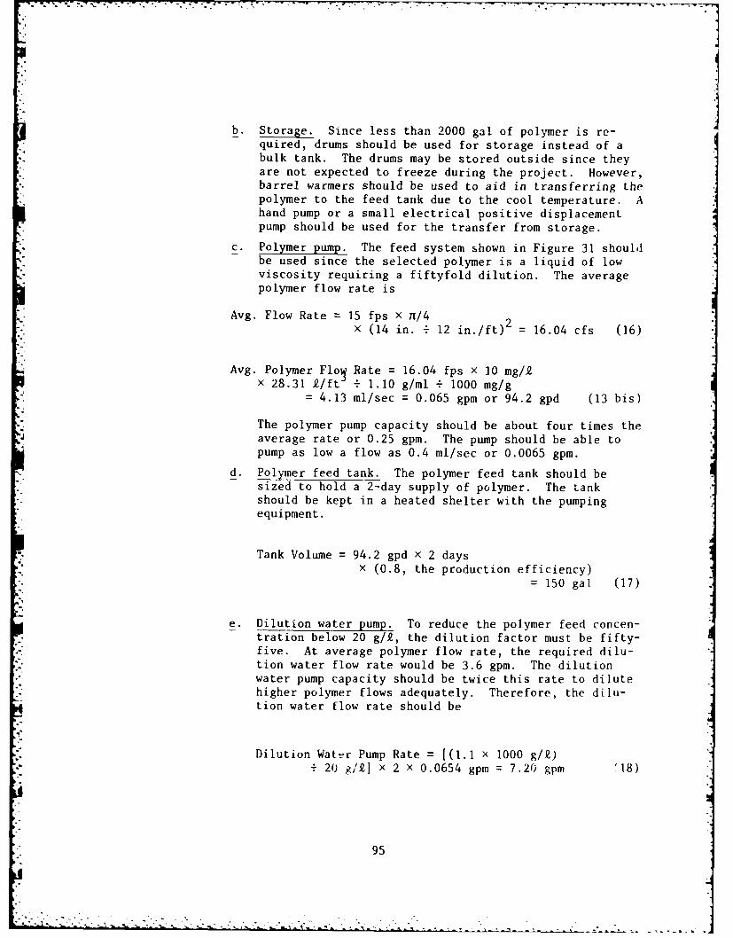
--+
b. Storage. Since less than 2000 gal of polymer is re-quired, drums should be used for storage instead of abulk tank. The drums may be stored outside since theyare not expected to freeze during the project. However,barrel warmers should be used to aid in transferring thepolymer to the feed tank due to the cool temperature. Ahand pump or a small electrical positive displacementpump should be used for the transfer from storage.
c. Polymer pump. The feed system shown in Figure 31 shouldbe used since the selected polymer is a liquid of lowviscosity requiring a fiftyfold dilution. The averagepolymer flow rate is
Avg. Flow Rate = 15 fps x n/4 2x (14 in. 12 in./ft) = 16.04 cfs (16)
Avg. Polymer Floi Rate = 16.04 fps x 10 mg/Ix 28.31 /ft 1.10 g/ml - 1000 mg/g
= 4.13 ml/sec = 0.065 gpm or 94.2 gpd (13 bis)
The polymer pump capacity should be about four times the4 average rate or 0.25 gpm. The pump should be able to
pump as low a flow as 0.4 ml/sec or 0.0065 gpm.
d. Polymer feed tank. The polymer feed tank should besized to hold a 2-day supply of polymer. The tankshould be kept in a heated shelter with the pumpingequipment.
Tank Volume = 94.2 gpd X 2 daysx (0.8, the production efficiency)
= 150 gal (17)
e. Dilution water pump. To reduce the polymer feed concen-tration below 20 g/i, the dilution factor must be fifty-five. At average polymer flow rate, the required dilu-tion water flow rate would be 3.6 gpm. The dilutionwater pump capacity should be twice this rate to dilutehigher polymer flows adequately. Therefore, the dilu-tion water flow rate should be
Dilution Water Pump Rate = [(1.1 x 1000 g/f)" 20 ?/k] x 2 x 0.0654 gpm 7.20 gpm '18)
95
II... . . . . . . .
The pump must deliver this flow rate and produce highpressure (60 psi) to force the viscous polymer solutionthrough the eductor, feed lines, and injector.
f. Feed lines. The size of the feed lines should be deter-mined by head loss analysis for pipe flow. This subjectis discussed in any fluid mechanics textbook or hydrau-lics handbook. The pipe diameter is dependent on theviscosity, flow rate, length of line, minor losses, andlosses through the eductor and injector. One-inch in-side diameter (ID) rubber hose or PVC pipe should beused for this example. The head loss would be less than30 psi.
Mixing system
182. The weir box and discharge culvert(s) should, if possible,
be designed to provide adequate mixing. A 2-ft drop between the water
surfaces of the first basin and the second basin is sufficient energy
for mixing if efficiently used. Mechanical mixers should be considered
if sufficient energy is unavailable. The design of mechanical mixing
systems has been presented by Jones, Williams, and Moore (1978) and will
not be duplicated here.
183. Weir. The weir should be designed to collect supernatant
from the primary containment area and to disperse the polymer thoroughly.
The weir box does not provide efficient mixing and, therefore, it is un-
desirable to lose all the energy of the water by a free fall into the
weir box. The system should provide a small drop into the weir box and
high head loss through the discharge culvert(s) between the primary and
secondary containment areas.
184. The weir box should be designed to prevent leakage; the bot-
tom of the box should be sealed. Only one section of the box needs to
be adjustable to the bottom of the box; this would minimize leakage.
Weir boards with tongue and groove joints would also decrease leakage.
The weir box should be submergible without the weir boards floating from
their positions. All sections of the weir should be level and at the
same elevation. An example is shown in Figure 34.
185. The height of the weir c;--st should be adjustable to stop
the flow when the flow is too low to treat or to maintain the flow in
order to keep treating when the dredge has stopped. The depth of flow
96
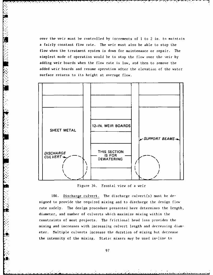
over the weir must be controlled by increments of I to 2 in. to maintain
a fairly constant flow rate. The weir must also be able to stop the
flow when the treatment system is down for maintenance or repair. The
simplest mode of operation would be to stop the flow over the weir by
adding weir boards when the flow rate is low, and then to remove the
added weir boards and resume operation after the elevation of the water
surface returns to its height at average flow.
12-IN. WEIR BOARDSSHEET METAL
SUPPORT BEAMS
THIS SECTIONDISCHARGE I OC U L V E R T . F IS F O R , - " " -CU--E" / - ,\ DEWATERING 00
-- II I
Figure 34. Frontal view of a weir
186. Discharge culvert. The discharge culvert(s) must be de-
signed to provide the required mixing and to discharge the design flow
rate safely. The design procedure presented here determines the length,
diameter, and number of culverts which maximize mixing within the
constraints of most projects. The frictional head loss provides the
*.-..mixing and increases with increasing culvert length and decreasing diam-
eter. Multiple culverts increase the duration of mixing but decrease
the intensity of the mixing. Static mixers may be used in-line to
97
increase the head loss of a culvert without increasing its length or de-
creasing its diameter. The use and design of static mixers will not be
discussed herein, but information on their use is available from their
manufacturers.
187. The design approach is to size the culvert for the maximum
flow rate ana the minimum available head and then to calculate the avail-
able mixing under average flow conditions. The maximum flow rate is
assumed to be the average dredge flow rate with continuous, 24-hr/day
production. The designer should also consider other possible sources of
inflow. The average flow at the weir is assumed to be the product of
average dredge flow rate and fractional production time ratio (generally
about 0.75 or 18 hr/day). In this manner the culvert will be able to
safely discharge the design flow. It is important to estimate the flow
rates fairly accurately in order to properly size the culvert. Under-
sizing can result in overtopping the dikes or in forcing the dredge to
operate intermittently. Oversizing can result in inadequate mixing.
The amount of mixing can be compared with the mixing requirements deter-
mined experimentally to evaluate the design. If inadequate, the de-
signer may wish to change the containment area design to provide a
greater head for mixing. The required head can be determined using the
design equations.
188. The design procedure is as follows (see Figure 26 for an
example weir mixing system):
a. Assume that the maximum flow rate is the average dredgeflow rate with continuous production, 24 hr/day.
b. Assume a 0.5-fL drop into the weir box under maximumflow.
c. Determine the difference in elevation Ah , in feet,between the water surface of the basins at their highestoperating levels from the design.
d. Let H , in feet, = Ah - 0.5 where H is the maximumpermissible head loss through the culvert at maximumflow.
e. Assuming a submerged inlet and outlet, and a corrugatedmetal culvert (though less head loss and better mixingfor low flows would be realized if the outlet were notsubmerged), then
98
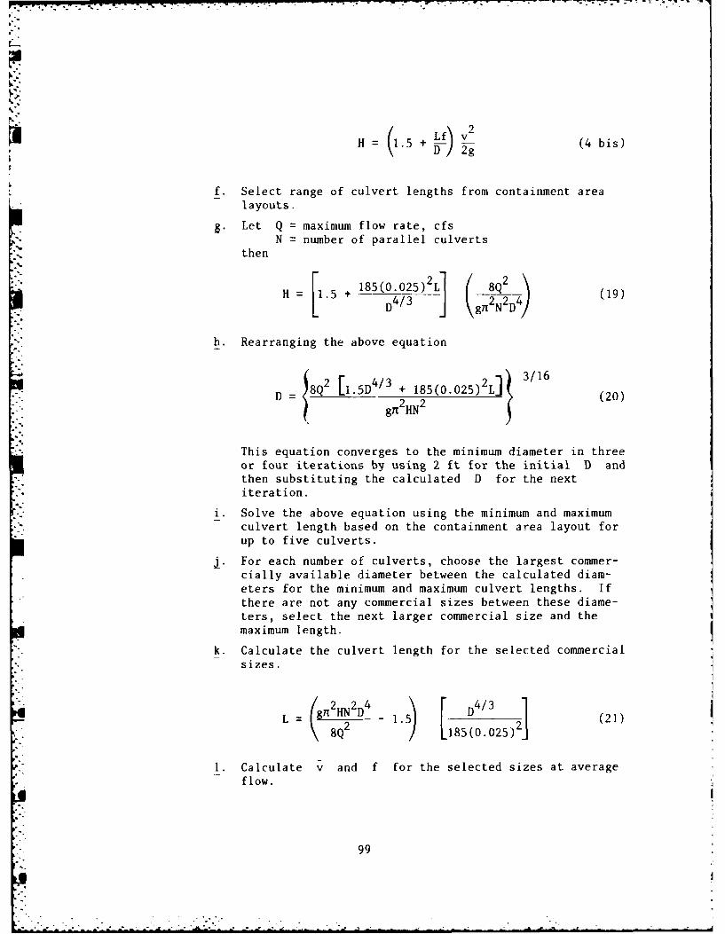
I'.
H =1 5 + 2g (4 bis)
f. Select range of culvert lengths from containment arealayouts.
. Let Q = maximum flow rate, cfsN = number of parallel culverts
then
185(0. 025) 2L][s - 4 3]8Q 2 4)(9
H 5+ D 43g7 2N2D4(9
h. Rearranging the above equation
(2[ /3D~ + 185(0. 025) 2 L] 3/16D= (20)
This equation converges to the minimum diameter in threeor four iterations by using 2 ft for the initial D andthen substituting the calculated D for the nextiteration.
i. Solve the above equation using the minimum and maximumculvert length based on the containment area layout forup to five culverts.
,. For each number of culverts, choose the largest commer-cially available diameter between the calculated diam-eters for the minimum and maximum culvert lengths. Ifthere are not any commercial sizes between these diame-ters, select the next larger commercial size and themaximum length.
k. Calculate the culvert length for the selected commercialsizes.
L = 8n2H2D4 I .) [85(0.025)2](11. Calculate v and f for the selected sizes at average
flow.
99
.o. .•. ... : . . . -•- ,. .. . - . .. .- * . .. -- ' ,. - ' i .' '. : *
v = 4 Q/nD 2 (22)
where
v = mean velocity at average flow, fps
= average flow rate, cfs
m. Calculate the mixing Gt of each design at averageflow.
ysfvLGt = ,-_23
where
Ys = specific weight, 62.4 lb/ft3
ps = absolute viscosity, 2.36 x 10 Ib-sec/ftat 60°F
n. Calculate the head loss at average flow and the maximumcarrying capacity of the culvert at a head of Ah todetermine limits of the design.
o. Select the best overall design based on mixing, cost,operating flexibility, etc.
189. Example culvert design. Given an 18-in.-diam dredge pipe-
line, a minimum head difference of 3 ft between the primary and secondary
cells, and a range of culvert lengths between 50 and 100 ft based on the
containment area design, the culvert design would proceed as follows:
a. Q = 15 fps x nT(18 in./12 in./ft) - 4 (24)- max
= 26.5 cfs
Qave = 26.5 cfs x (Production ratio, 0.75) (25)
= 19.9 cfs
b. Ah = 3 ft
H = 3 ft - 0.5 ft = 2.5 ft (26)
100
-A
c. The calculated minimum diameters for the followinglengths and numbers of culverts are:
N L, ft D, ftD, in.
1 50 2.23 26.81 100 2.44 29.32 50 1.67 20.02 100 1.85 22.23 50 1.42 17.03 100 1.57 18.84 50 1.26 15.14 100 1.41 16.95 50 1.15 13.85 100 1.29 15.5
d. The selected commercial sizes and calculated lengths are:
N D, in. LI ft
1 27 54.12 21 69.3
3 18 73.34 18 100.0
5 15 83.0
e. The friction factor and velocity at average flow are:
N D, in. fps f
1 27 5.00 0.08822 21 4.14 0.09593 18 3.75 0.10104 18 2.82 0.10105 15 3.24 0.1073
f. Mixing at average flow:
N D, in. L, ft G(sec ) t(sec) Gt
1 27 54.1 449 10.8 48552 21 69.3 400 16.7 6690
3 18 73.3 382 19.5 74704 18 100.0 249 35.5 88305 15 83.0 346 25.6 8870
g. Head loss at average flow:
H = 1.41 ft
h. Flow through a completely submerged weir:
Q = 29.0 cfs
,.1 o 1 .lo
I . . .. - , J\ i,
...---. ..
i. Generally, a Gt of about 8000 provides adequate mix-ing for chemical treatment. In this example, eitherthree 18-in.-diam, 73-ft-long culverts, four 18-in.-diam, 100-ft-long culverts or five 15-in.-diam, 83-ft-long culverts could be used. However, four 18-in.-diamculverts would be the best design since it would pro-vide considerably more mixing than three culverts andabout the same mixing as five culverts. Also, thisdesign would provide better mixing at lower flow rates.
Secondary containment area
190. Design approach. The secondary area must be designed to pro-
vide adeqLate detention time for good settling and sufficient volume forstorage of settled material. The total volume of the cell is the sum of
the ponded volume and the storage volume. The required ponded volume is
a function of the hydraulic efficiency of the cell and the flow rate.
The storage volume is dependent on the solids concentration entering the
basin, the depth of the cell, the total volume to be treated, the flow
rate, and the mud pumping schedule.
191. Ponded volume. Effective settling requires a ponded depth
of 2 to 3 ft and a minimum of 20 min of detention. Due to short-
circuiting, the mean detention time should be at least 60 min and the
theoretical detention time of the ponded volume should be at least
150 min. The shape of the cell should have a length-to-width ratio of
at least 3:1 to reduce short-circuiting.
192. Storage volume. The settling properties of flocculated
dredged material resulting from chemical clarification have not been
well defined. Solids concentration or density profiles have been mea-
sured at only one field site as presented earlier in this report. The
settled material was very fluid and, as such, did not clog the inlet
culvert though settled material accumulated near the inlet to a depth
I ft higher than the top of the culvert. The momentum of the inflow was
capable of keeping the inlet clear of material. Resuspended material
settled rapidly in the basin. The concentration of settled material at
the interface between the supernatant and settled layer was 50 g/Q, and| the concentration increased with increasing depth at a rate of 25 g/k/ft.
Therefore, deeper basins stored more material in a given volume due to
L102
compaction. The concentration of the material increased rapidly upon
dewatering.
193. Knowing the average available depth of the secondary basin,
the total storage requirements can be estimated as follows:
a. The total mass of material to be stored M or pumpedfrom the secondary area is
M, g = (Primary effluent conc.- Secondary effluent conc., g/Q)
>Y (Volume to be treated, k) (2
b. The average concentration of settled material Cs is
C, g/2 = [2 x 50 g/2 + 25 g/k/ftx (Average depth of storage, ft)] 2 (28)
c. Total volume of settled treated material V iss
Vs, P= (M, g) (Cs,
V, ft3 (Vs, ) 28.31 k/ft3 (29;
d. The maximum area required A is5
A acre = (V, ft 3 (Average depth of storage, ft)2
43,560 ft /acre (30)
194. Ponded area. The required volume V and area A forp p
ponding are
- VP = (Average flow rate, cfs) x 9000 sec (31)
A = V (Average depth of ponding, ft) (32)p p
*195. Design area. The containment area should be designed to
have a total depth of the sum of the ponded depth and the depth of
103
storage. The area of the cell should be the larger of the areas; re-
quired for ponding and for storage. If the area required for storage is
greater than the area required for ponding, the depth of ponidirig ('an he
reduced but niot below a depth of 2 to 3 ft, thereby increasing the
available depth of storage. If the area for storage is still greater,* the only way to reduce the area requirements further would be to remove
settled treated material from the basin into the primary containment
area to decrease the required storage volume. In the overall basin de-
sign, it is important to use the greatest practical depth and to opti-
* mize its use to provide good mixing through the discharge culvert, ponid-
ing for good settling, and storage for treated material. To minimize
the size of the secondary area and to maximize the energy available for
mixing, the secondary area should be used only for temporary storage ex-
cept for small one-time projects. Therefore, the settled treated mate-
rial should be regularly removed from the basin. This approach would
also facilitate dewatering and recurring use of the area for chemical
treatment.
196. Mud pumping. If the settled material is to be pumped, the
required pumping rate would be
Mass Pumping Rate, g/day = (Influent conc., g/-aEffluent conc., g/ x (Average flow rate, cfs)
3x 28.31 2/ft x (Seconds of production per day) (33)
Volumetric Pumping Rate, ft 3 /day
* =(Mass Pumping Rate, g/day) +[2 x 50 g/2 + 25 g/k/ft
x (Average depth of storage, ft)] x 2 (34)
197. Inlet baffles. The inlet hydraulics of the secondary area
can have a significant effect on settling performance. Inlet affles
as shown in Figure 26 can reduce the effects of short-circuitinb and
turbulent flow and assist in distributing the flow laterally. The eaf-
fles should be placed about one diameter directly in front of the inlet.
104
r.
L
The baffle should be at least two diameters wide and may be either slot-
ted or solid. Slotted baffles are better and may be made of 4- by 4-in.
wooden posts spaced several inches apart. The main purpose of the inlet
baffles is to dissipate the kinetic energy of the incoming water and the
velocity of the flow toward the weir.
198. Effect on dewatering. Design of the secondary area must
consider dewatering of the primary area. If the primary area is to be
dewatered using the primary weir box to drain the water, the elevation
of the surface of the water or stored material in the secondary area
must be lower than the final elevat:ion of the stored material to be at-
tained during dewatering. The elevation difference should be at least
2 ft if the drainage is to be treated. This point is demonstrated in
Figure 35.
199. There are several alternatives that can be used to provide
for dewatering:
a. The secondary area can be constructed at a lowerelevation.
b. The settled, treated material stored in the secondaryarea can be dewatered and thereby consolidated first.
c. The material can be pumped out of the secondary area.
d. The water can be pumped out of the primary area.
e. A special drainage structure can be constructed to drainthe primary cell.
f. A channel can be cut through the settled material in thesecondary area to permit drainage through the basin.
The best approach is dependent on site- and project-specific considera-
tions. The effect of treatment on dewatering of the primary area is
just one example showing that the designer should consider the entire
disposal operation when designing the treatment system. Treatment
should not be tacked on a disposal operation as an afterthought.
200. Design example. Given the following project information, the
settling basin size would be determined as follows:
a. Project information.
Primary effluent solids conc. 2 g/k
Secondary effluent solids conc. 50 mg/i
105
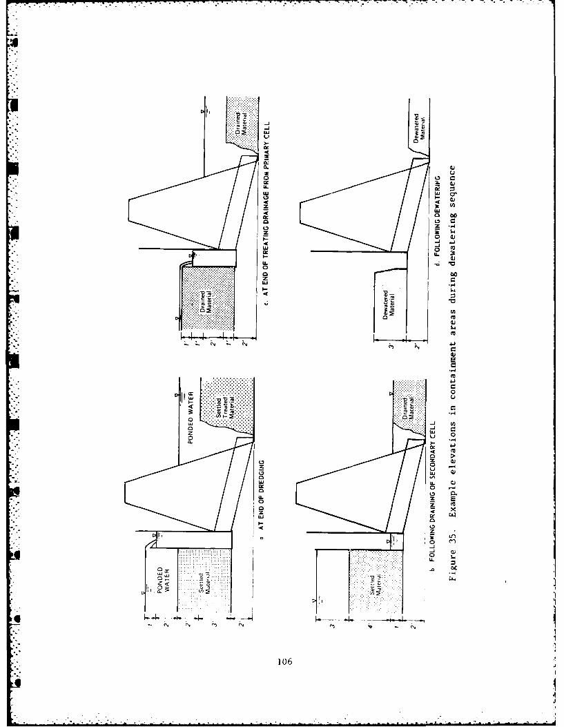
X.l -J
(U
U.. -
LU
4 4J
4 I -4
000
0 u0 . L
44
'U 0 )
0K 0 -a
zz
Lu
0 3C
1060
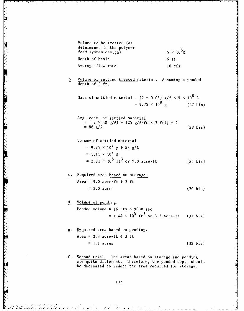
Volume to be treated (asdetermined in the polymerfeed system design) 5 x 10 k
Depth of basin 6 ft
Average flow rate 16 cfs
b. Volume of settled treated material. Assuming a pondeddepth of 3 ft,
Mass of settled material = (2 - 0.05) g/k x 5 x 108
= 9.75 x 10⁸ g (27 bis)
Avg. conc. of settled material= [(2 x 50 g/9) + (25 g/k/ft x 3 ft)] - 2= 88 g/2 (28 bis)
Volume of settled material
= 9.75 x 10⁸ g + 88 g/g
1.11 X 10⁷ 9
3.91 x 105 ft3 or 9.0 acre-ft (29 bis)
c. Required area based on storage.
Area = 9.0 acre-ft + 3 ft
= 3.0 acres (30 bis)
d. Volume of ponding.
Ponded volume = 16 cfs x 9000 sec
= 1.44 x 10 ft3 or 3.3 acre-ft (31 bis)
e. Required area based on ponding.
Area = 3.3 acre-ft 3 ft
= 1.1 acres (32 bis)
f. Second trial. The areas based on storage and pondingare quite different. Therefore, the ponded depth shouldbe decreased to reduce the area required for storage.
107
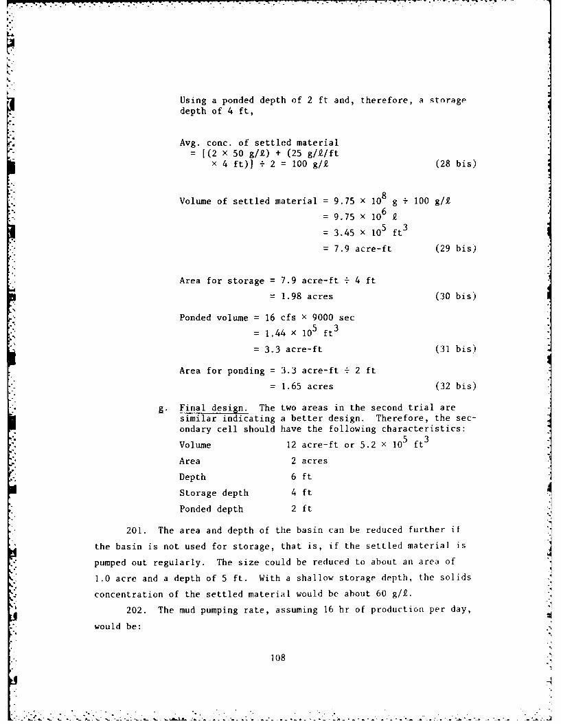
Using a ponded depth of 2 ft and, therefore, a storagedepth of 4 ft,
Avg. conc. of settled material
[ (2 x 50 g/Q,) + (25 g/.e/ftx 4 ft)) - 2 = 100 g/9 (28 bis)
8Volume of settled material = 9.75 x 10 g 100 g/9
= 9.75 x 10⁶ 9
5 3
= 3.45 x 10 5ft3
=7.9 acre-ft (29 bis)
Area for storage = 7.9 acre-ft 4 ft
= 1.98 acres (30 bis)
Ponded volume = 16 cfs x 9000 sec
5, 3
= 1.44 X 10 ft
= 3.3 acre-ft (31 bis)
Area for ponding = 3.3 acre-ft 2 ft
= 1.65 acres (32 bis)
Final design. The two areas in the second trial aresimilar indicating a better design. Therefore, the sec-ondary cell should have the following characteristics:
Volume 12 acre-ft or 5.2 x 105 ft 3
Area 2 acres
Depth 6 ft
Storage depth 4 ft
Ponded depth 2 ft
201. The area and depth of the basin can be reduced further if
the basin is not used for storage, that is, if the settled material is
pumped out regularly. The size could be reduced to about an area of
1.0 acre and a depth of 5 ft. With a shallow storage depth, the solids
concentration of the settled material would be about 60 g/.
202. The mud pumping rate, assuming 16 hr of production per day,
would be:
108
the~~~~ - AA 2-i*sntuedfrsoae ha s ftestte aeili
--..
Solids Pumping Rate = (2.0 - 0.05) g/23
x 28.31 2/ft x 16 cfsx 16 hr/day x 3600 sec/hr
= 5.09 X 10⁷ g/day (33 bis)
Volumetric Pumping Rate = 5.09 x 10⁷ g/day - 60 g/2
= 8.5 x 10⁵ 2/day
= 0.347 cfs or 156 gpm (34 bis)
General design considerations
203. Shelter. A building should be provided to house the equip-
ment and to furnish shelter for the operators. An 8- by 12-ft portable
building is sufficient unless the polymer storage tank and dilution
tanks must be housed.
204. Equipment. The equipment should be simple, rugged, heavy-
duty, continuous-duty, low-maintenance equipment. Backup equipment must
be provided for all essential components.
205. Safety. Good lighting must be provided for the entire work
area. The weir must be furnished with a walkway and railings. Provi-
sions should be made for safe, simple adjustments of the weir boarding.
206. Costs. These cost estimates are based on the field demon-
strations described in Part IV of this report. The principal costs are
construction, labor, and polymer. The costs are presented in 1981
dollars.
207. The one-time, project-independent engineering and design
costs are
Flocculant screening $2,000
Design and equipment selection $3,000
208. The major nonexpendable equipment costs are given below, but
these costs can be much larger if the polymer must be housed cr if the
polymer must be prediluted prior to feeding.
Two polymer feed pumps withmotors and controllers $ 3,400
Two dilution water pumps withmotors $ 1,200
109
Two generators $ 5,000
One mud pump $10,000
One portable building $ 5,000
Polymer and dilution waterfeed lines, intake, andinjection rig $ 1,000
One mixing eductor $ 150
Other miscellaneous equipment $ 1,000
Vehicle $ 8,000
Portable turbidimeter $ 800
Total $35,550
Based on a 2-year design life, the prorated monthly cost would be about
$1,500/month. These costs are slightly dependent on the size of the
project.
209. The cost of expendable supplies is dependent on the project
size.
Fuel $400/month
Polymer $0.70/lb
210. The labor requirements are dependent on the required ef-
fluent quality. To achieve consistently good removals, an operator
should attend the system during all operating hours. The operator re-
quires only minimal training but good mechanical aptitude. For the
majority of the time, the operator will be idle and free to do other
tasks. Labor costs for full-time operators would be about
Labor costs = $15/hr x 1.5 x (Number of production hours)
211. The total cost excluding costs of construction (secondary
cell and outlet structure, access road, land) would be about $0.08/yd
to $0.25/yd of in situ sediment to be dredged or $35 to $100 per hour
of production. The rate of cost is dependent on the size of the proj-
ect, the production rate, and the dosage of polymer. The approximate
breakdown of variable costs are given below for eight cases.
110
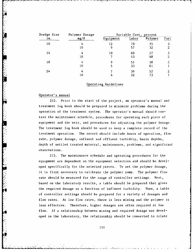
Dredge Size Polymer Dosage Variable Cost, percentin. mg/ Equipment Labor Polymer Fuel
10 4 12 70 15 310 9 57 32 2
14 4 10 60 27 310 7 43 48 2
18 4 9 51 38 210 5 33 61 1
24 4 7 39 52 210 4 22 73 1
Operating Guidelines
Operator's manual
212. Prior to the start of the project, an operator's manual and
treatment log book should be prepared to minimize problems during the
operation of the treatment system. The operator's manual should con-
tain the maintenance schedule, procedures for operating each piece of
equipment and the weir, and procedures for adjusting the polymer dosage.
The treatment log book should be used to keep a complete record of the
treatment operation. The record should include hours of operation, flow
rate, polymer dosage, influent and effluent turbidity, basin depths,
depth of settled treated material, maintenance, problems, and significant
observations.
213. The maintenance schedule and operating procedures for the
equipment are dependent on the equipment selection and should be devel-
oped specifically for the selected pieces. To set the polymer dosage,
it is first necessary to calibrate the polymer pump. The polymer flow
rate should be measured for the range of controller settings. Next,
based on the laboratory results, a table should be prepared that gives
the required dosage as a function of influent turbidity. Then, a table
of controller settings should be prepared for a variety of dosages arid
flow rates. At low flow rates, there is less mixing and the polymer is
less effective. Therefore, higher dosages are often required at low
flow. If a relationship between mixing and required dosage was devel-
oped in the laboratory, the relationship should be converted to relate
' 111
-. . . . . . . . .. . . ... . . - .
flow rate and dosage so the operator can readily adjust the dosage. The
required dosages must be verified during the start of operation and the
values in the tables must be adjusted accordingly. After verification
the operator would only have to measure the influent turbidity and flow
rate to determine the controller setting for the polymer pump.
Field dosage verification
214. During verification of the required dosages, the effectiveness
of a particular dosage can be evaluated immediately by grabbing a sample
of treated suspension from the end of the discharge culvert connecting
the two containment areas and running a column settling test on the sam-
ple. If the supernatant is clear after 10 min of settling, the dosage
should be decreased until the supernatant is slightly cloudy. Better
clarification will be achieved in the settling basin where the material
can flocculate. This is especially true when the system has been oper-
ating continuously for a long period. After selecting a dosage, the
effluent turbidity should be monitored to determine whether the dosage
should be adjusted further. The dosage should be minimized to reduce
chemical costs, but the effluent quality should not be allowed to dete-
riorate beyond the effluent requirements.
Flow measurement
215. The flow rate can be estimated by measuring the depth of
water flowing over the weir crest and the weir length. Assuming that
the entire weir crest is at the same elevation, the flow rate can be
computed as follows (Rehbock 1912; Rao 1975; Streeter 1971):
H = (h/0.85) 12 in./ft (35)
where
H = static head over weir crest, ft
h = depth of flow over weir, in.
€. (H3/2
Q = 3.33 B(H) (36)
112
ii .... . . -
- - ,. . . ...
r. -
where
Q = flow rate, cfs
B = weir length, ft
The above equations apply for sharp- and narrow-crested rectangular
weirs that are not submerged.
216. A table should be generated relating the depth of flow over
the weir h and the flow rate Q and included in the operator's manual.
The weir length should be measured and not taken from design drawings to
ensure accuracy. With this table the operator would easily be able to
estimate the flow rate by measuring the depth of flow without performing
any difficult computations or requiring additional information. The
operator should measure the depths at several locations along the weir
crest and average the resulting flow rates to determine the overall flow
rate. This method would minimize the estimating errors caused by an
unlevel or uneven weir crest.
217. The weir crest may become submerged at flow greater than
20 percent above the average. The actual flow rate that submerges the
weir is dependent on the weir length and culvert design. The flow rate
over submerged weirs is controlled by discharge capacity of the culvert.
Weir operation
218. The weir must be properly operated to maintain good mixing
conditions. The weir crest must be kept sufficiently high to maintain
the required difference in elevation between the water surtaces of the
two containment areas. The weir should also be used to maintain the re-
quired flow rate for good mixing. When the flow decreases below the
minimum rate for good mixing, the operator should either lower the weir
crest by 1 or 2 in., increasing the flow to its average rate, or raise
the weir crest sufficiently to stop the flow.
219. The minimum flow rate is based on the experimentally deter-
mined minimum acceptable mixing Gt for effective treatment. The mini-
mum flow can be determined as follows:
113
-I- . - ~ --- --- ~~. t t~. -. - - -
mmt 2"" min avgG- min / (37)Qmm QavgI
-"avg/
An example computation is given below.
Given: Average flow = 25 cfsGt of average flow = 9000Minimum acceptable Gt = 6000
The minimum allowable flow is
Qmin =25 cfs \9000
= 11.1 cfs
220. In general, the weir crest should be operated at the highest
practical elevation and the primary containment area should be allowed
to fill before any water is discharged over the weir and treatment is
started. This would maximize the depth and provide the best conditions
for mixing, settling, and storage. Maintaining the maximum ponded depth
in the primary area also minimizes the turbidity to be treated and there-
fore reduces the required polymer dosage.
Other considerations
221. General operation. During the project, the primary and sec-
ondary effluent turbidity, and flow rate should be measured at least six
times per day and the polymer flow rate should be adjusted as needed.
Each piece of equipment should be inspected regularly, particularly the
water intake, injection rig, and pumps. The fuel and chemical levels
should also be checked as required. Regular maintenance must be per-
formed throughout the project. The buildup of settled treated material
should be followed and the material should be pumped out of the basin as
the storage volume is depleted.
222. Leakage. The operator should try to eliminate leakage
through the weir when the treatment system is turned off. The flow rate
of the leakage is too low to treat, but after a couple of days of down-
time the leakage can completely exchange the contents of the secondary
114
. .. . . .. .
area if left unchecked. Since it is untreated, the effluent quality
will deteriorate markedly.
223. Dewatering. At the end of the project, the treatment system
can be used to treat the drainage from the primary containment area dur-
ing dewatering. The elevation of the interface of the settled material
in the primary area must be greater than the elevation of the water sur-
face of the secondary area. Therefore, the secondary area must be de-
watered first to compact the settled treated material and to provide the
depth required to treat the drainage at the lower weir height. It is
possible that treated material may need to be pumped from the secondary
area before the primary area can be dewatered through the weir.
115
. . . . j
. .... 1
PART VII: CONCLUSIONS AND RECOMMENDATIONS
Conclusions
224. Chemical clarification is an effective treatment method to
remove suspended solids and turbidity from the effluent of a fine-
grained dredged material containment area. Low viscosity, highly ca-
tionic liquid polymers were found to be the most effective chemicals and
the simplest to use. The treatment method can be adapted to work within
the constraints of a normal disposal operation. The treatment system
can be simplified to use little equipment, mainly pumps, thereby making
operation easy. Mixing can be performed in the weir structure without
mechanical equipment. A small secondary containment area can be used
for settling and storage, eliminating the need for a clarifier and
sludge handling equipment.
225. The operation of the system is simple. The main duties of
the operators are maintenance, filling fuel and polymer feed tanks, in-
spection, adjusting polymer feed rate, and controlling the height of the
weir crest to maintain good mixing. Heavy duty, continuous rated, reli-
able equipment minimizes operating problems.
226. A well-designed treatment system is capable of producing an
effluent that averages a suspended solids concentration of less than
50 mg/2 and a turbidity of less than 50 NTU during continuous operation.
Under adverse conditions, the effluent suspended solids concentration
may be as high as 200 mg/i and the turbidity as high as 200 NTU.
227. The jar test procedure described in this report is capable
of determining the most effective flocculant, required dosage, mixing
requirements, acceptable polymer feed concentration, and effects of var-
iable primary effluent solids concentration. The required polymer dos-
age is directly related to the turbidity to be treated and inversely
related to the amount of mixing available at the weir.
228. The costs of chemical treatment are highly variable and de-
*O pendent on the specifics of the dredging project. Excluding the costs
of the secondary containment area and weir structure, the costs may
116
range from about $0.08/yd to $0.25/yd 3 of in situ sediment dredged de-
pending on the production rate, dosage, and treatment design. The major
costs are labor, polymer, and construction.
229. The dosage required to treat drt'iged material slurries by
injecting polymer into the dredge pipeline is proportional to the non-
settleable turbidity or clay fraction of freshwater sediments. The same
loading, milligrams polymer per gram of clays, is required for pipeline
injection as for treatment at the weir. The required dosage would be
much higher since the concentration of clays in a dredge discharge is
much greater than in the effluent from a primary containment area. The
variablity of the influent solids concentration would also require that
a higher average dosage be used to compensate for periods of high solids
concentration. The optimum injection location appears to be about 500 ft
from the discharge point. Pipeline injection would greatly increase
polymer costs but significantly reduce labor and construction costs.
This treatment method may be applicable to small projects at freshwater
sites that have a small clay fraction.
230. Finally, a better treatment system design can be achieved if
treatment is considered (luring the planning of the disposal operation.
In this manner, the cont.,inment area can be laid out to increase the
hydraulic efficiency of the basins and to utilize the available depth
efficiently for mixing, ponding, and storage.
Recommenda t ions
231. Based on the results of this study, the following recommenda-
tions are made:
a. The effects of mixing provided by weir structures de-signed ajs recommended in this report on the effective-ness of poiymer dos.i,,es shoiild be examined and corre-lated with the effe, ts from laboratory tests. This wor.(is needed to verify the mixing design and to scale-upprocediirs based on the calculation of GL values.
b. Column settling tests should be performed on treatedmaterial from the efflent of a primary containment areato examine the eflects of treatment on the concentrationlof settled material.
117
I
c. The effects of treatment on the dewatering of settledmaterial in the secondary basin should be examined.
d. The pipeline injection treatment method should be care-fully studied in the laboratory before being further ap-plied in the field. Laboratory procedures should bedeveloped to test the method and to develop design param-eters. Detailed polymer screening should be performed onseveral freshwater and saltwater sediment slurries thatcover a wide range of clay concentrations.
e. Column settling tests and consolidation tests shouldbe performed on the treated slurries to examine the ef-fects of polymer addition on settleability and storagerequirements.
f. After laboratory testing, a full-scale, long-term demon-stration of pipeline injection should be performed todetermine the effects on the effluent quality and thedensity profiles of the settled material.
118
t'" "
-- , .,.- .-. .. ---.
REFERENCES
Alexander, A. E., and Johnson, P. 1949. Colloid Science, Oxford Uni-versity, London.
American Public Health Association, American Water Works Association,and Water Pollution Control Federation. 1976. Standard Methods for th,Examination of Water and Wastewater, 14th ed., Washington, D. C.
Black, A. P., et al. 1957. "Review of the Jar Test," American WaterWorks Association Journal, Vol 49, pp 1414-1424.
Headquarters, Department of the Army. 1970. "Laboratory Soils Testing,"Engineer Manual EM 1110-2-1906, Washington, D. C.
Headquarters, Department of the Army. 1980. "Guidelines for Designing,Operating and Managing Dredged Material Containment Areas," EngineerManual EM 1110-2-5006, Washington, D. C.
Hudson, H. E., Jr. 1981. Water Clarification Processes PracticalDesign and Evaluation, Van Nostrand Reinhold, New York.
Jones, R. H., Williams, R. R., and Moore, T. K. 1978. "Development julApplication of Design and Operation Procedures for Coagulation ofDredged Material Slurry and Containment Area Effluent," TechnicalReport D-78-54, U.S. Army Engineer Waterways Experiment Station, CE,Vicksburg, Miss.
La Mer, V. K. 1964. "Coagulation Symposium Introduction," Journal ofColloid Science, Vol 19, pp .119-232.
Matijevi6, E., and Allen, L. II. 1969. "Interactions of Colloidal Dis-persions with Electrolytes, ltivironmental Science and Technology, Vol 3,pp 264-268.
Rao, N. W. L,. 1975. "Theory of Weirs," Advances in Hydroscience,Vol 10, Academic Press, New York.
Rehbock, T. 1912. "Der Alefliuse ulne Wehre Nerschiedener Querschnitte,"Z. Ver. Deut. Architekten Ing-Ver. As cited in Gallagher, B. 1978."Investigation of Containment Area Design to Maximize Settling Effec- 14
tiveness," Technical Report D)-78-12, U.S. Army Engineer WaterwaysExperiment Station, CE, Vicksburg, Miss.
Streeter, V. L. 1971. FluiI M,,c-h-an ics., 5th ed., McGraw-Hill, New York.
U.S. Army Engineer Waterways Experiment Station, CE. 1953. "TheU <,ii*ied SoiI Cl.,ss t ication )vtem," Technical Memorandum No. 3-357,
I uk~lbirg, Miss.
V.!I ()lphe , II. 196 3. An In ru'.iiction_ to Clay _Colloid Chemistry, Inter-.S,- I ., New York.
Walski, T. M., and Schroeder, P. R. 1978. "Weir Design to MaintainEffluent Quality from Dredged Material Containment Areas," TechnicalReport D-78-18, U.S. Army Engineer Waterways Experiment Station, CE,Vicksburg, Miss.
119
.4
'_ " ] i : . : " ' - . . . . . • . :. . . . . .. ' - • "
Wang, C. C., and Chen, K. Y. 1977. "Laboratory Study of Chemical* Coagulation as a Means of Treatment for Dredged Material," Technical
- Report D-77-39, U.S. Army Engineer Waterways Experiment Station, CE,Vicksburg, Miss.
V
120
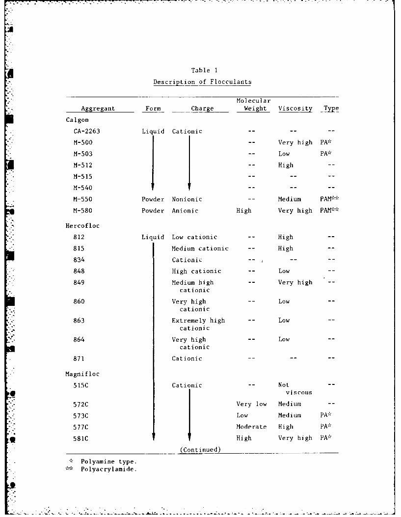
Table 1
Description of Flocculants
MolecularAgg re gant Form - Charge Weight Visosiy Type
Calgon
CA-2263 Liquid Cationic - --
M-500 -- Very high PA*
M-503 -- Low PA*
M-S512 -- High--
M-515
M-540
M-550 Powder Nontionic -- Medium PAM**
M-580 Powder Anionic High Very high PAM*
Hercofloc
812 Liquid Low cationic -- High -
815 Medium cationic -- High -
934 Cationic - --
848 High cationic -- Low
849 Medium high -- Very high -
cationlic
860 Very high -- Low -
cationic
863 Extremely high -- Low
cationi c
864 Very high -- Low -
cationic
871 Cationic - --
Magnifloc
515C Cationic -- Not -
* viscous
57 2C Very low Medium -
573C Low Medium PA
5 77C Moderate High PA*
581C High Very high PA*
(Continued)__ ________
* Polyamine type.Polyacrylamide.
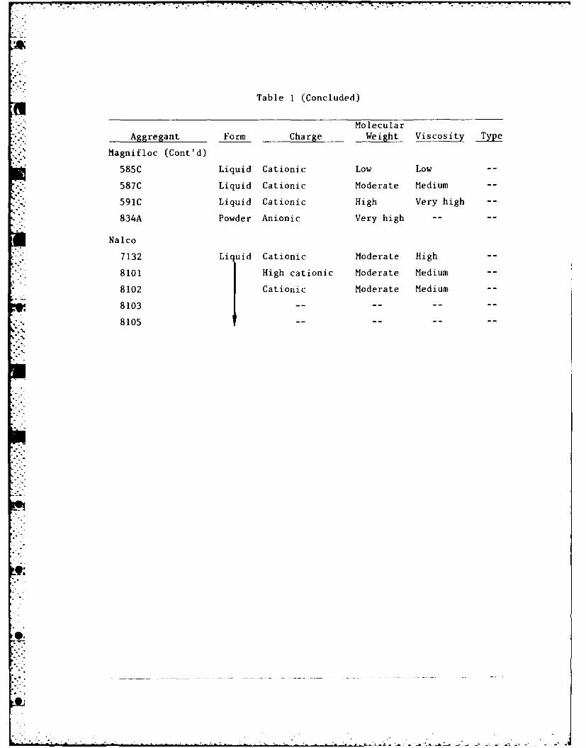
Table I (Concluded)
Molecular*Aggregant Form Charge Weight Viscosity Type
Magnifloc (Cont'd)
585C Liquid Cationic Low Low--
* .587C Liquid Cationic Moderate Medium -
591C Liquid Cationic High Very high -
*834A Powder Anionic Very high --
Nalco
*.7132 Liquid Cationic Moderate High -
-8101 I High cationic Moderate Medium -
8102 Cationic Moderate Medium -
8103 -
8105
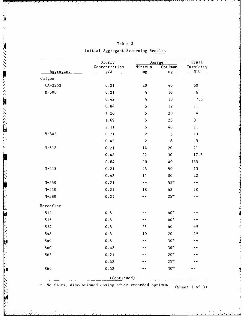
Table 2
Initial Aggregant Screening Results
Slurry Dosage FinalConcentration Minimum Optimum Turbidity
Aggregant g/. mg mg NTUP9Calgon
CA-2263 0.21 20 40 60
M-500 0.21 4 10 6
0.42 4 10 7.5
0.84 5 12 11
1.26 5 20 4
1.69 5 35 31
2.11 5 40 11
M-503 0.21 2 3 13
0.42 2 6 9
M-512 0.21 14 20 21
0.42 22 30 17.5
0.84 20 40 155
M-515 0.21 25 50 13
0.42 11 80 22
M-540 0.21 -- 55* --
M-550 0.21 18 42 78
M-580 0.21 -- 25* --
Hercofloc
812 0.5 -- 40* --
815 0.5 -- 40* --
834 0.5 35 40 69
848 0.5 10 20 49
849 0.5 -- 30* --
860 0.42 -- 30* --
863 0.21 -- 20* --
0.42 -- 25* --
864 0.42 -- 30* --
(Continued) _"
No flocs, discontinued dosing after recorded optimum. ( e o• (Sheet I of 3)

Table 2 (Continued)
Slurry Dosage Final
Concentration Minimum Optimum TurbidityAggregant g/f mg mg NTU
Hercofloc (Cont'd)
871 0.5 30 40 83
Magnifloc
515C 0.21 35 55 10
0.42 -- 40* --
572C 0.21 3 10 6
0.42 5 15 6
0.42 3 7 20
0.84 4 12 11
1.26 4 16 33
1.69 5 30 2
2.11 7 35 37
573C 0.42 2 4 15
1.26 2 12 12
577C 0.42 2 6 16
1.26 4 10 10
2.11 4 20 9
581C 0.21 5 8 21
0.42 6 10 23
0.84 7 20 --
1.26 7 35 28
1.69 6 35 20
2.11 10 40 26
585C 0.42 4 12 12.I
1.26 6 12 45
587C 0.42 4 10 11
1.26 5 20 13
591C 0.21 6 10 16
0.42 7 15 10
(Continued) .___
No flocs, discontinued dosing after recorded optimum.(Sheet 2 of 3)
LII
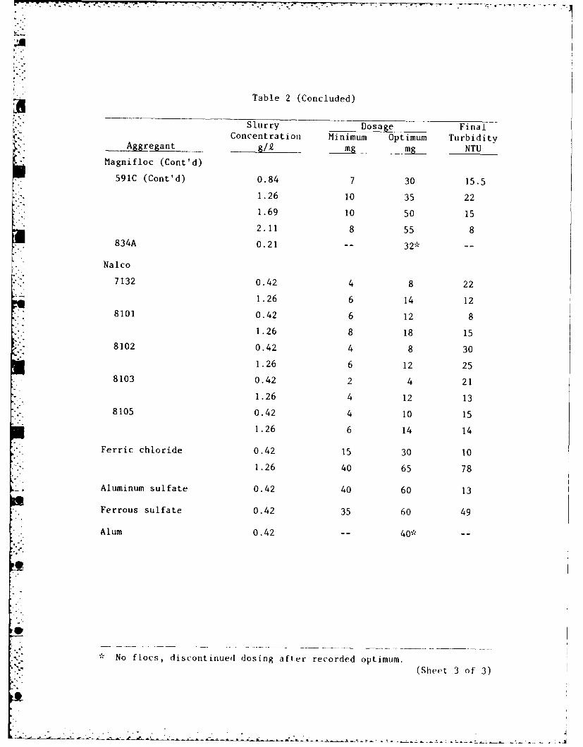
Table 2 (Concluded)
' Slurry Dosage FinalConcentration Minimum Optimum Turbidity
Aggregant -g/ mg mg NTU
Magnifloc (Cont'd)
. 591C (Cont'd) 0.84 7 30 15.5
1.26 10 35 221.69 10 50 15
2.11 8 55 8834A 0.21 -- 32* --
Nalco
. 7132 0.42 4 8 22
1.26 6 14 12
8101 0.42 6 12 8
1.26 8 18 158102 0.42 4 8 30
1.26 6 12 25
8103 0.42 2 4 21
1.26 4 12 13
8105 0.42 4 10 15
1.26 6 14 14
Ferric chloride 0.42 15 30 10
1.26 40 65 78
Aluminum sulfate 0.42 40 60 13
Ferrous sulfate 0.42 35 60 49
Alum 0.42 -- 40* --
No flocs, discontinued dosing after recorded optimum.
(Slheet 3 of 3)
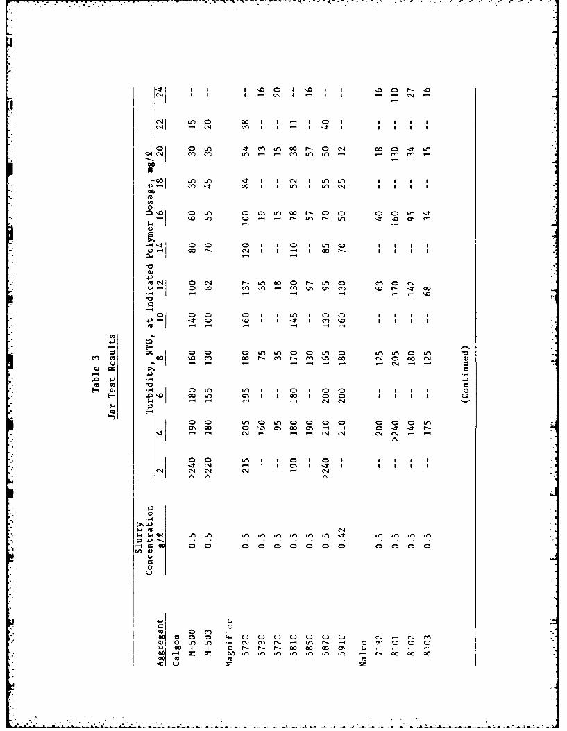
C,4 "oL~ C LID Lo a r- Cl oC14 -4
co CN :n '0TL Ln
00) ir, 0 0' , V)0 r- 00 00D 1D -,t
- '0 in 0C ,- r- in r-- in -T '0 m' C
1-4-4
u000 0n Y) I n 0 7 w n 0I
4-) -T C -t c '
0D C'D .- in .1 ' u l 0
0(A 00 \D CY 0 r - C ) \40 0' al w. r-U-4 -4-4" - -4 C-4 -
41 4
00 0) 0I a CE-4 ~ ~ ~ ~ ~ Cl D Lr n : ' (=w- C- C4,
cc E
ON 00 0 a% i 00 ON 0 Qn IT 0I -4 r-4 4 1 ' -1 -1 - CN 4
T-41
c124
00
01 a 0 4.4 0 u n 0 0 0 0 0 0 C- in- Ca' CO Lt) at'1 CI M - - 0 m 4 '4C C
'4 - - r - - C'0 e00 ON. U '
0 0 n In In 0n In 0n I
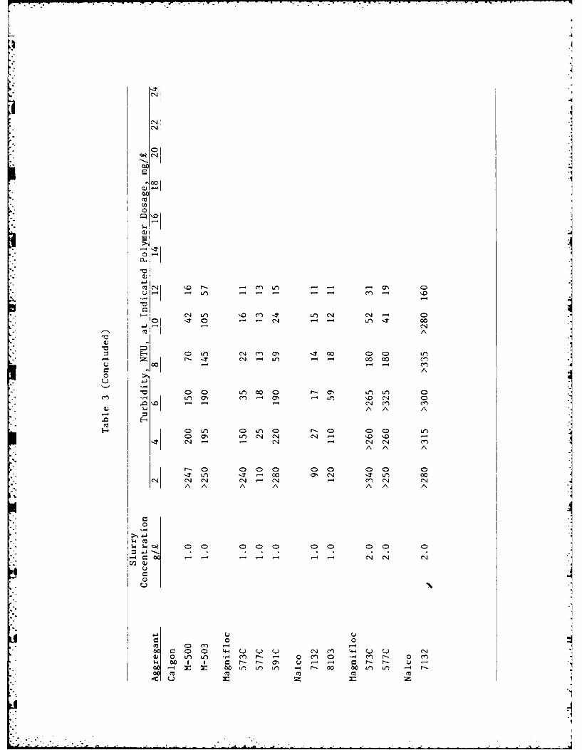
C144
0 *10I
$-4
u .- -- - -cn - \.O
't N 0 . C 14 Lt)CJ - 00
I A
0 tt0 M ~ 0 t C
M4 Ln ON -n -I -n C CO4
U* CO - - -MA A A
0
r-
0 ( r 0 0 00 0') 1-4 N -'0 '.1
C 0 0 000 00 00 0ic -
" I - r " u - - r-4 Ln -n - - - r- N N Nn i .
jO Ca
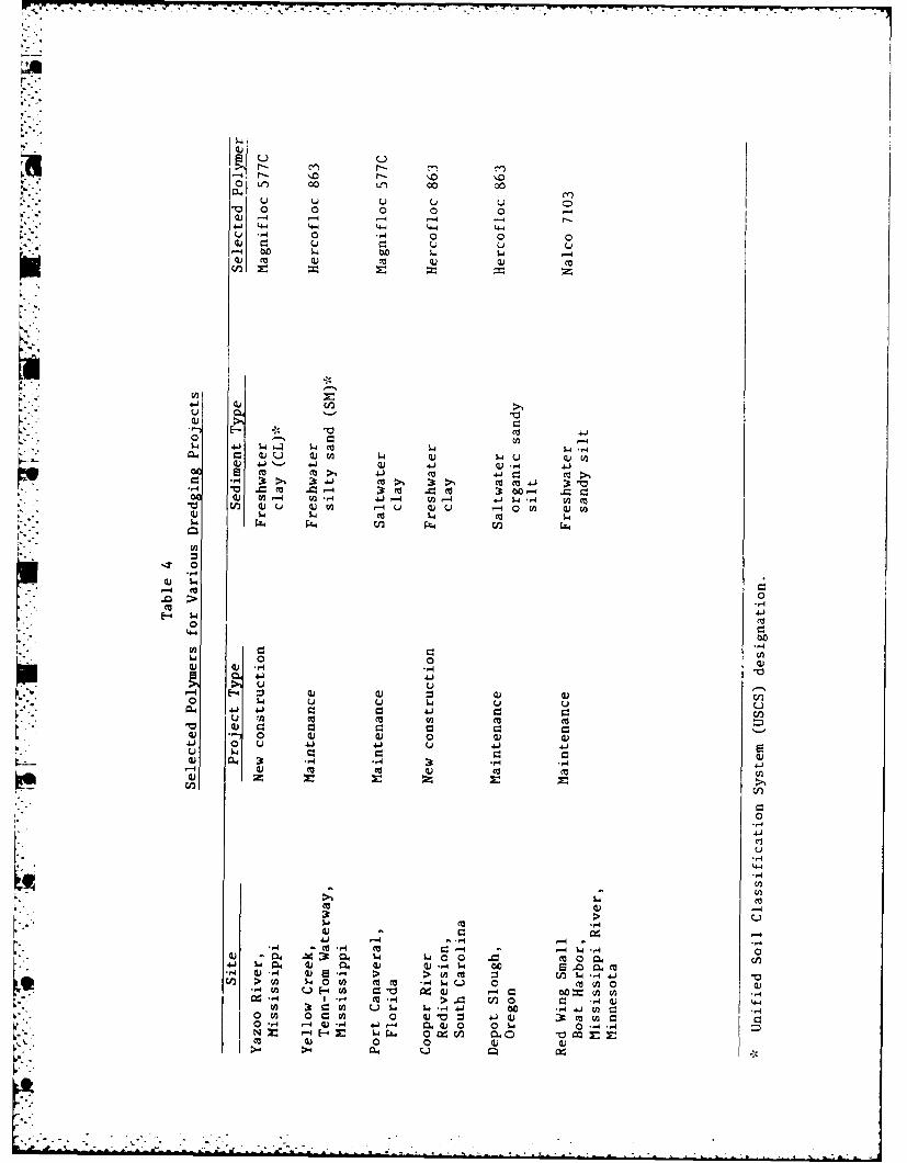
O Lfn 00 tn 00
a~0 0 0 04,; -. 4 -4
Q -4 0 .4 0 0 0U) r. u u
1-4 00 $ O 4 4P4) mi Q)m
W:
4- 441
-44 31. AU 413; c m
V) aj u ai ( - ) ui -4 .c.()r
-. 5-0
41)
41.
4 4.j 41)U r. C30
a4 it.' .4 .,q . 4
-4
di -4C 4 4.-4
- 4.) rm5- -44 >. >.A5-4 44,-4 w 0C.- )0 -P-4 W 0 m 4.4 0cn 4) -4 a- 00 =~ V) V
0C1 r. c 0 qj 41-4) (0". 04 4)- .) 0d 0 0 S-4 0-4 -4N i 0- 0 X i (n .
0 ..
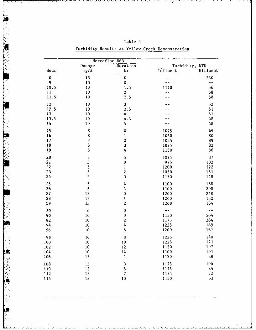
Table 5
Turbidity Results at Yellow Creek Demonstration
Hercofloc 863Dosage Duration Turbidity, NTU
Hour mg/I hr Influent Effluent
0 13 0 -- 2509 10 0 -- --
10.5 10 1.5 1110 5611 10 2 -- 6811.5 10 2.5 -- 58
12 10 3 -- 5212.5 10 3.5 -- 51
" 13 10 4 -- 5113.5 10 4.5 -- 4814 10 5 -- 48
15 8 0 1075 4916 8 1 1050 8017 8 2 1025 8918 8 3 1075 8219 8 4 1150 86
20 8 5 1075 8721 5 0 975 10222 5 1 1200 12223 5 2 1050 15124 5 3 1150 148
25 5 4 1100 16826 5 5 1100 20027 13 0 1200 24828 13 1 1200 13229 13 2 1200 164
30 0 0 -- --
90 10 0 1150 50492 10 2 1175 36494 10 4 1225 189
" 96 10 6 1200 161
98 10 8 1225 140
100 10 10 1225 121102 10 12 1150 107104 10 14 1100 101106 13 1 1150 88
108 13 3 1175 104110 13 5 1175 84112 13 7 1175 72115 13 10 1150 63
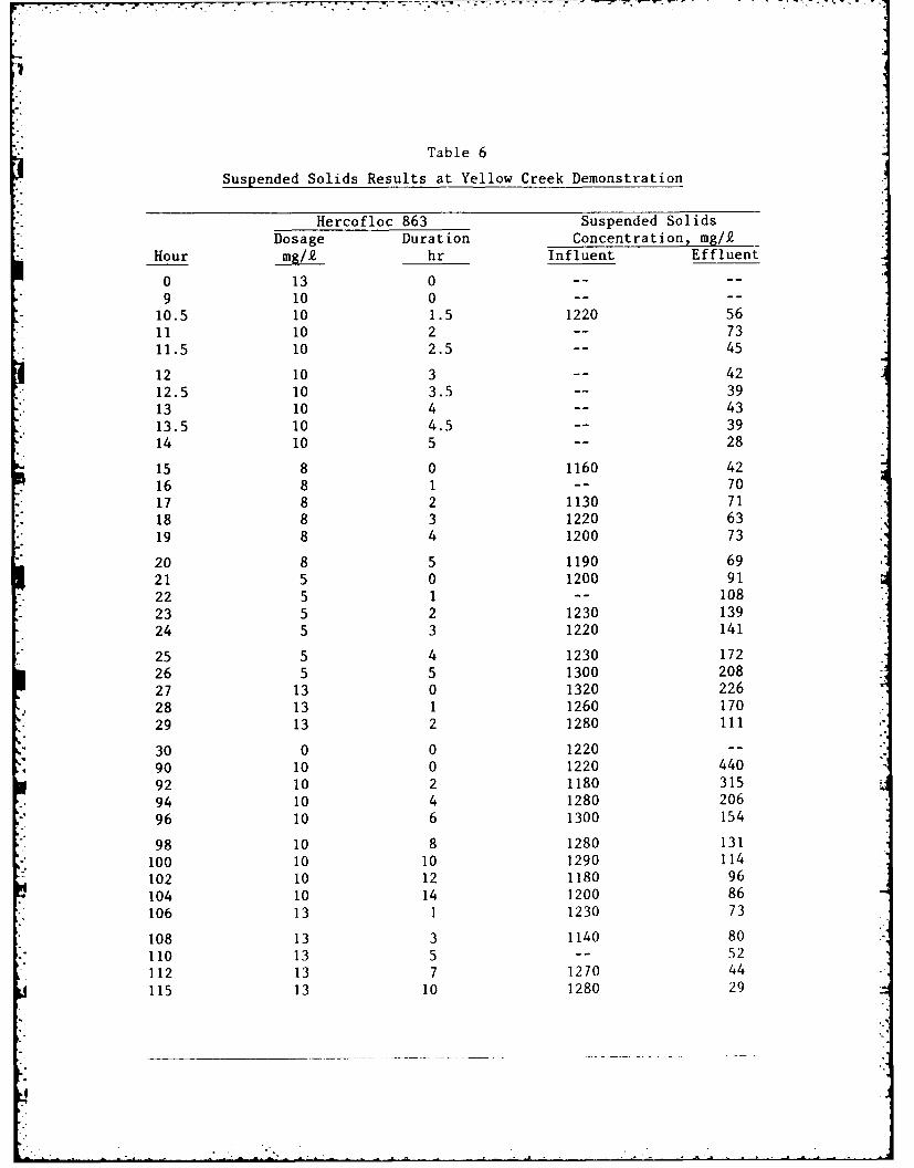
Table 6
Suspended Solids Results at Yellow Creek Demonstration
Hercofloc 863 Suspended Solids
Dosage Duration Concentration, mg/2Hour mg/.£ hr Influent Effluent
0 13 0 --
9 10 0 -- --
10.5 10 1.5 1220 5611 10 2 -- 73
11.5 10 2.5 -- 45
12 10 3 -- 42
12.5 10 3.5 -- 39
13 10 4 -- 43
13.5 10 4.5 -- 39
14 10 5 -- 28
15 8 0 1160 4216 8 1 -- 70
17 8 2 1130 7118 8 3 1220 6319 8 4 1200 73
20 8 5 1190 6921 5 0 1200 9122 5 1 -- 10823 5 2 1230 13924 5 3 1220 141
25 5 4 1230 17226 5 5 1300 20827 13 0 1320 226
28 13 1 1260 17029 13 2 1280 111
30 0 0 1220 --
* 90 10 0 1220 440
92 10 2 1180 31594 10 4 1280 206
96 10 6 1300 154
98 10 8 1280 131100 10 10 1290 114
102 10 12 1180 96
104 10 14 1200 86
106 13 1 1230 73
108 13 3 1140 80
110 13 5 -- 52
112 13 7 1270 44
115 13 10 1280 29
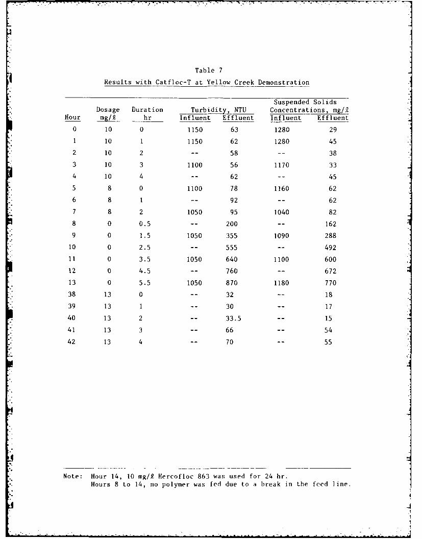
Table 7
Results with Catfloc-T at Yellow Creek Demonstration
Suspended SolidsDosage Duration Turbidity, NTU Concentrations, mg/2
Hour mg/Q hr Influent Effluent Influent Effluent
0 10 0 1150 63 1280 29
1 10 1 1150 62 1280 45
2 10 2 -- 58 -- 38
3 10 3 1100 56 1170 33
4 10 4 -- 62 -- 45
5 8 0 1100 78 1160 62
6 8 1 -- 92 -- 62
7 8 2 1050 95 1040 82
8 0 0.5 -- 200 -- 162
9 0 1.5 1050 355 1090 288
10 0 2.5 -- 555 -- 492
11 0 3.5 1050 640 1100 600
12 0 4.5 -- 760 -- 672
13 0 5.5 1050 870 1180 770
38 13 0 -- 32 -- 18
39 13 1 -- 30 -- 17
40 13 2 -- 33.5 15
41 13 3 -- 66 -- 54
42 13 4 -- 70 -- 55
Note: Hour 14, 10 mg/k Hercofloc 863 was used for 24 hr.Hours 8 to 14, no polymer was fed due to a break in the feed line.
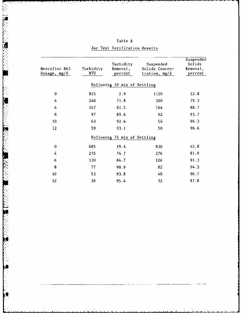
Table 8
Jar Test Verification Results
SuspendedTurbidity Suspended Solids
Hercofloc 863 Turbidity Removal, Solids Concen- Removal,Dosage, mg/. NTU percent tration, mg/i percent
Following 10 min of Settling
0 825 2.9 1120 22.8
4 240 71.8 300 79.3
6 157 81.5 164 88.7
8 97 88.6 92 93.7
10 63 92.6 54 96.3
12 59 93.1 50 96.6
Following 75 min of Settling
0 685 19.4 830 42.8
4 215 74.7 276 81.0
6 130 84.7 126 91.3
8 77 90.9 82 94.3
10 53 93.8 48 96.7
12 39 95.4 32 97.8
'q
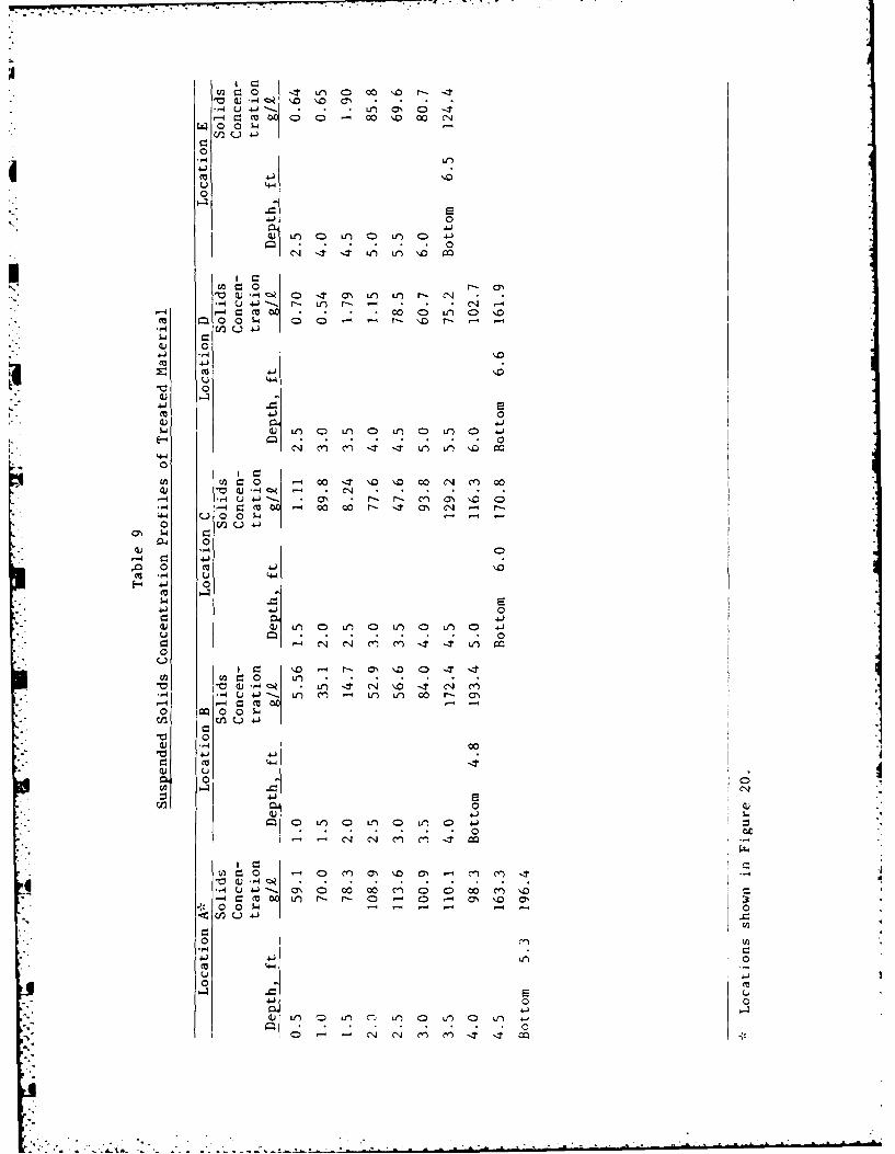
I U - r,--q 0 m C) CO 0 00 \.o W- C-
w ~1~'0 0. -
-2 Lf a f0 -
0
0
00
m 0 7 a f0~r
mH4J-.. r- ) LI, rl Z- =
14 -4 U C Co) (31 0: r,:
CC c ~ 0 0 0 0w'. r . - -
-4I
1-4 0 -
HV 0
.41
00
-4 .H 0J--4 4 ' . -. r- 1a' '0
N C C4 h-) M. -T -t LO W-
0 0
0~4
(C .14 00m~- 4--4
(U *
0
0~ I n 0 n I,0
UV ' W 4 I C. c), -0 C) '0 - 0 N Cl)0~-. m / Cl-LL, I, C r- a'
0 C 0w:r
'V 0
41 .. 0 CaV 4)
N. pl n I '
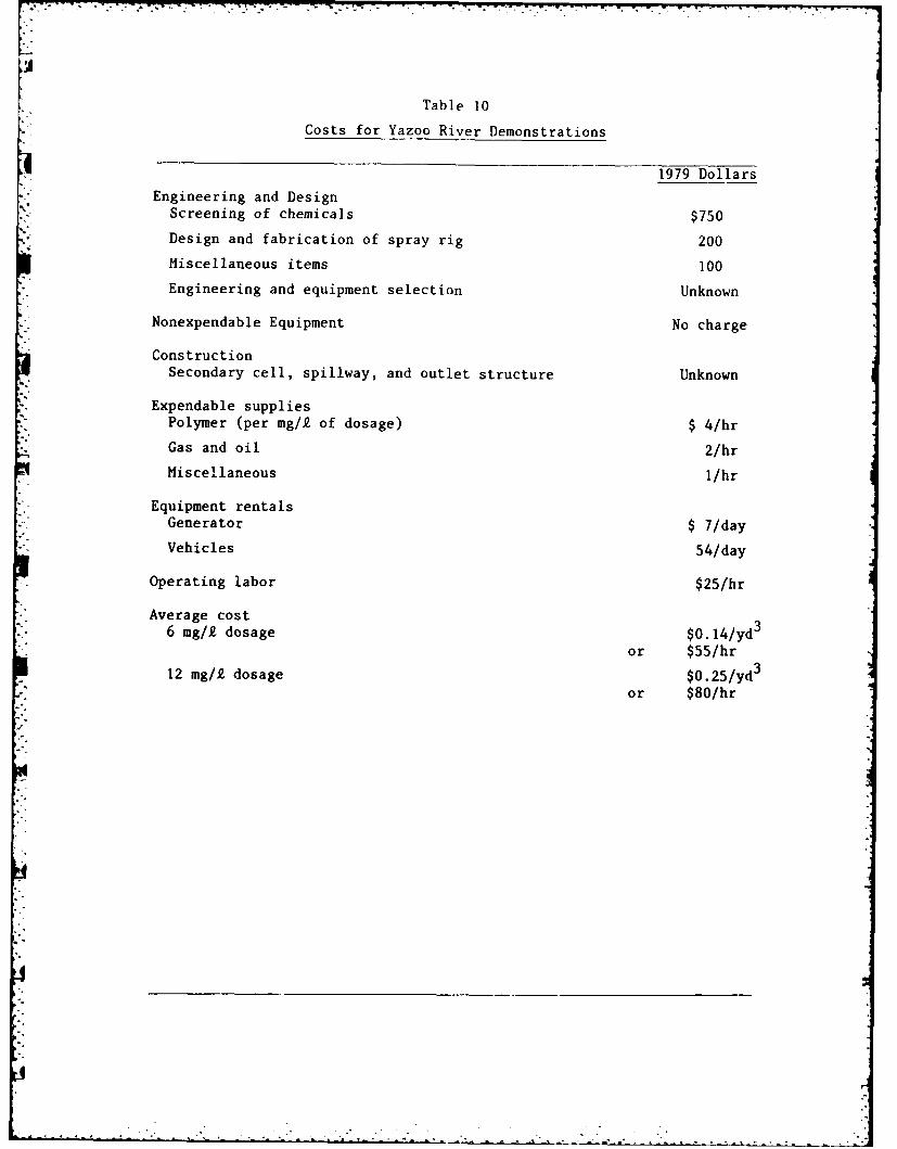
Table 10
Costs for Yazoo River Demonstrations
1979 Dollars
Engineering and DesignScreening of chemicals $750
Design and fabrication of spray rig 200
Miscellaneous items 100
Engineering and equipment selection Unknown
Nonexpendable Equipment No charge
ConstructionSecondary cell, spillway, and outlet structure Unknown
Expendable supplies
Polymer (per mg/2 of dosage) $ 4/hr
Gas and oil 2/hr
Miscellaneous 1/hr
Equipment rentals
Generator $ 7/day
Vehicles 54/day
Operating labor $25/hr
Average cost6 mg/k dosage $0.14/yd3
or $55/hr
12 mg/i dosage $0.25/yd3
or $80/hr
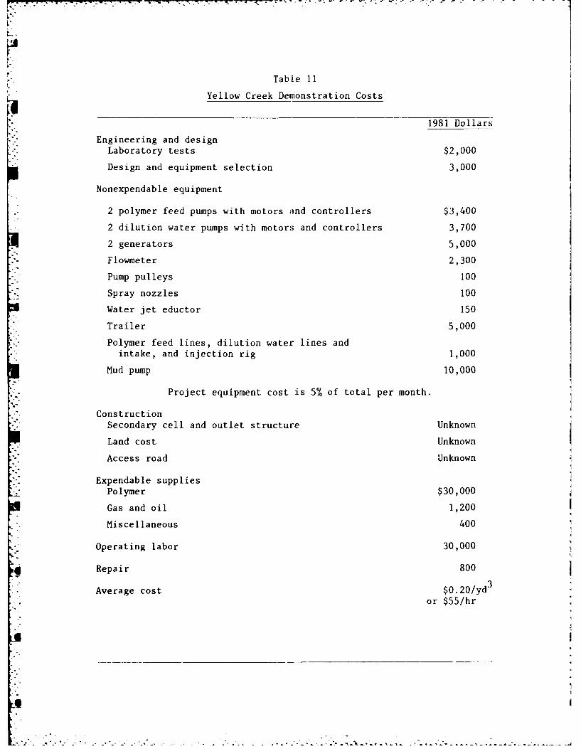
i L '. - . i - -. "-- L -- " "
" '' " " "- . . . ... .. "t " - " ' -
Table 11
Yellow Creek Demonstration Costs
1981 Dollars
Engineering and designLaboratory tests $2,000
Design and equipment selection 3,000
Nonexpendable equipment
2 polymer feed pumps with motors and controllers $3,400
2 dilution water pumps with motors and controllers 3,700
2 generators 5,000
Flowmeter 2,300
Pump pulleys 100
Spray nozzles 100
Water jet eductor 150
Trailer 5,000
Polymer feed lines, dilution water lines andintake, and injection rig 1,000
Mud pump 10,000
Project equipment cost is 5% of total per month.
ConstructionSecondary cell and outlet structure Unknown
Land cost Unknown
Access road Unknown
Expendable supplies
Polymer $30,000
Gas and oil 1,200
Miscellaneous 400
Operating labor 30,000
* Repair 800
Average cost $0.20/yd3
or $55/hr
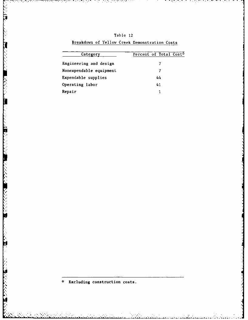
Table 12
Breakdown of Yellow Creek Demonstration Costs
Category Percent of Total Cost*
Engineering and design 7
Nonexpendable equipment 7
Expendable supplies 44
Operating labor 41
Repair 1
*Excluding construction costs.
S. °.,
- , ,
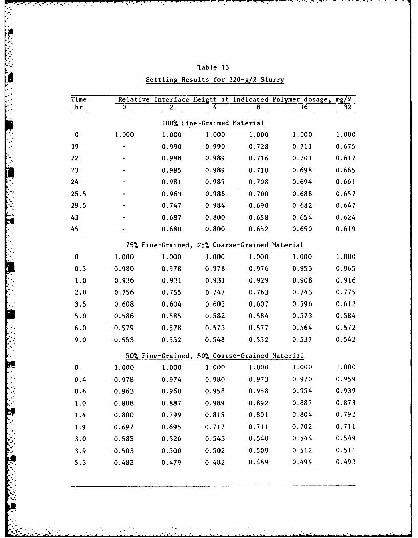
Table 13
Settling Results for 120-g/.e Slurry
Time Relative Interface Height at Indicated Polymer dosage, mg/khr 0 2 4 8 16 32
100% Fine-Grained Material
0 1.000 1.000 1.000 1.000 1.000 1.000
19 - 0.990 0.990 0.728 0.711 0.675
22 - 0.988 0.989 0.716 0.701 0.617
23 - 0.985 0.989 0.710 0.698 0.665
24 - 0.981 0.989 0.708 0.694 0.661
25.5 - 0.963 0.988 0.700 0.688 0.657
29.5 - 0.747 0.984 0.690 0.682 0.647
43 - 0.687 0.800 0.658 0.654 0.624
45 - 0.680 0.800 0.652 0.650 0.619
75% Fine-Grained, 25% Coarse-Grained Material
0 1.000 1.000 1.000 1.000 1.000 1.000
0.5 0.980 0.978 0.978 0.976 0.953 0.965
1.0 0.936 0.931 0.931 0.929 0.908 0.916
2.0 0.756 0.755 0.747 0.763 0.743 0.775
3.5 0.608 0.604 0.605 0.607 0.596 0.612
5.0 0.586 0.585 0.582 0.584 0.573 0.584
6.0 0.579 0.578 0.573 0.577 0.564 0.572
9.0 0.553 0.552 0.548 0.552 0.537 0.542
50% Fine-Grained, 50% Coarse-Grained Material
0 1.000 1.000 1.000 1.000 1.000 1.0000.4 0.978 0.974 0.980 0.973 0.970 0.959
0.6 0.963 0.960 0.958 0.958 0.954 0.939
1.0 0.888 0.887 0.989 0.892 0.887 0.873
1.4 0.800 0.799 0.815 0.801 0.804 0.792
1.9 0.697 0.695 0.717 0.711 0.702 0.711
3.0 0.585 0.526 0.543 0.540 0.544 0.549
3.9 0.503 0.500 0.502 0.509 0.512 0.511
5.3 0.482 0.479 0.482 0.489 0.494 0.493
m-3
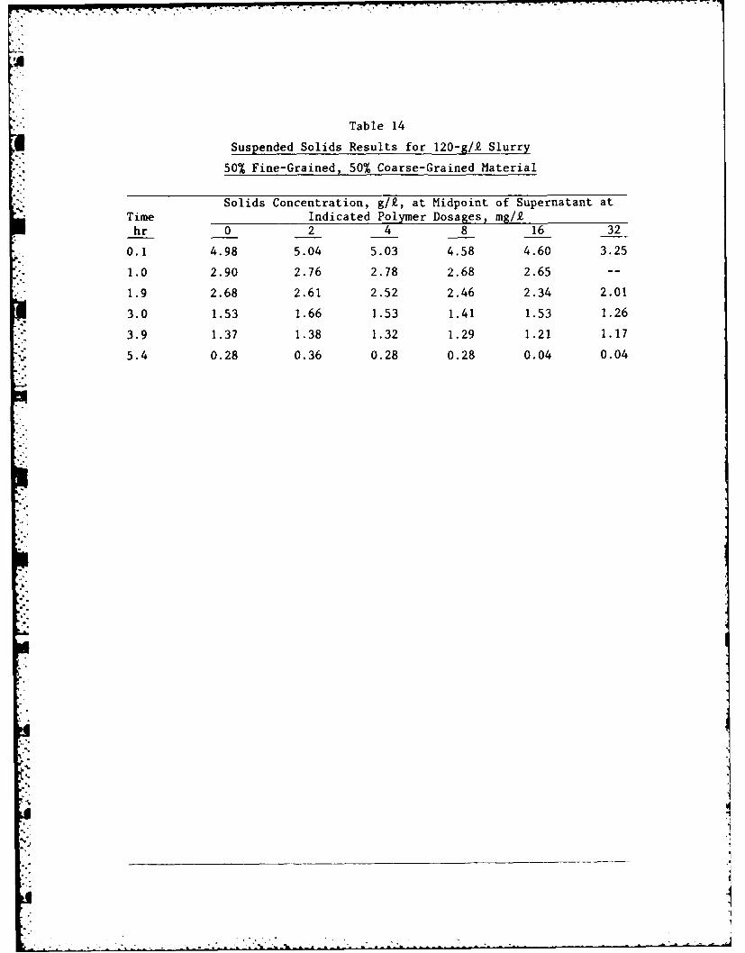
Table 14
Suspended Solids Results for 120-g/.e Slurry
50% Fine-Grained, 50% Coarse-Grained Material
Solids Concentration, g/g, at Midpoint of Supernatant atTime Indicated Polymer Dosages, mg/.ehr 0 2 4 8 16 32
0.1 4.98 5.04 5.03 4.58 4.60 3.25
1.0 2.90 2.76 2.78 2.68 2.65 --
1.9 2.68 2.61 2.52 2.46 2.34 2.01
3.0 1.53 1.66 1.53 1.41 1.53 1.26
3.9 1.37 1.38 1.32 1.29 1.21 1.17
5.4 0.28 0.36 0.28 0.28 0.04 0.04
p°'A
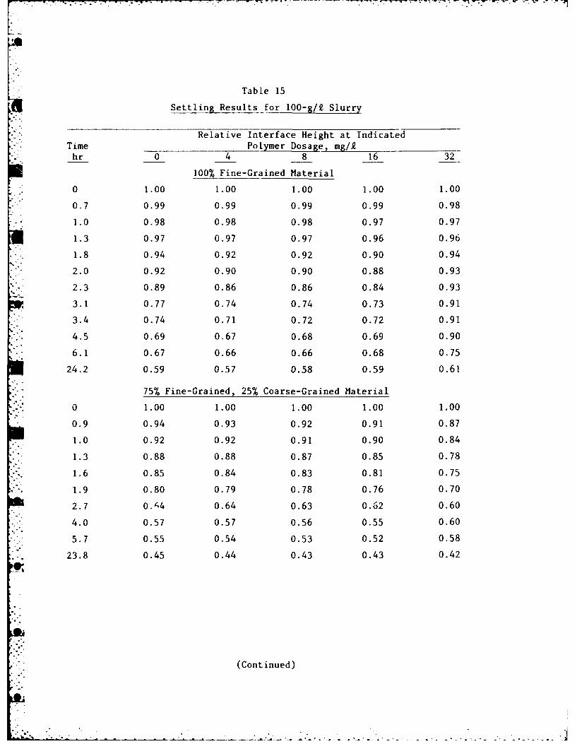
Table 15
Settling Results for 100-g/2 Slurry
Relative Interface Height at IndicatedTime Polymer Dosage, mg/2hr 0 4 8 16 32
100% Fine-Grained Material
0 1.00 1.00 1.00 1.00 1.00
0.7 0.99 0.99 0.99 0.99 0.98
1.0 0.98 0.98 0.98 0.97 0.97
1.3 0.97 0.97 0.97 0.96 0.96
* 1.8 0.94 0.92 0.92 0.90 0.94
2.0 0.92 0.90 0.90 0.88 0.93
2.3 0.89 0.86 0.86 0.84 0.93
3.1 0.77 0.74 0.74 0.73 0.91
- 3.4 0.74 0.71 0.72 0.72 0.91
4.5 0.69 0.67 0.68 0.69 0.90
6.1 0.67 0.66 0.66 0.68 0.75
24.2 0.59 0.57 0.58 0.59 0.61
75% Fine-Grained, 25% Coarse-Grained Material
0 1.00 1.00 1.00 1.00 1.00
0.9 0.94 0.93 0.92 0.91 0.87
* 1.0 0.92 0.92 0.91 0.90 0.84
1.3 0.88 0.88 0.87 0.85 0.78
1.6 0.85 0.84 0.83 0.81 0.75
1.9 0.80 0.79 0.78 0.76 0.70
2.7 0.A4 0.64 0.63 0.62 0.60
4.0 0.57 0.57 0.56 0.55 0.60
5.7 0.55 0.54 0.53 0.52 0.58
23.8 0.45 0.44 0.43 0.43 0.42
o'e
• ° (Continued)
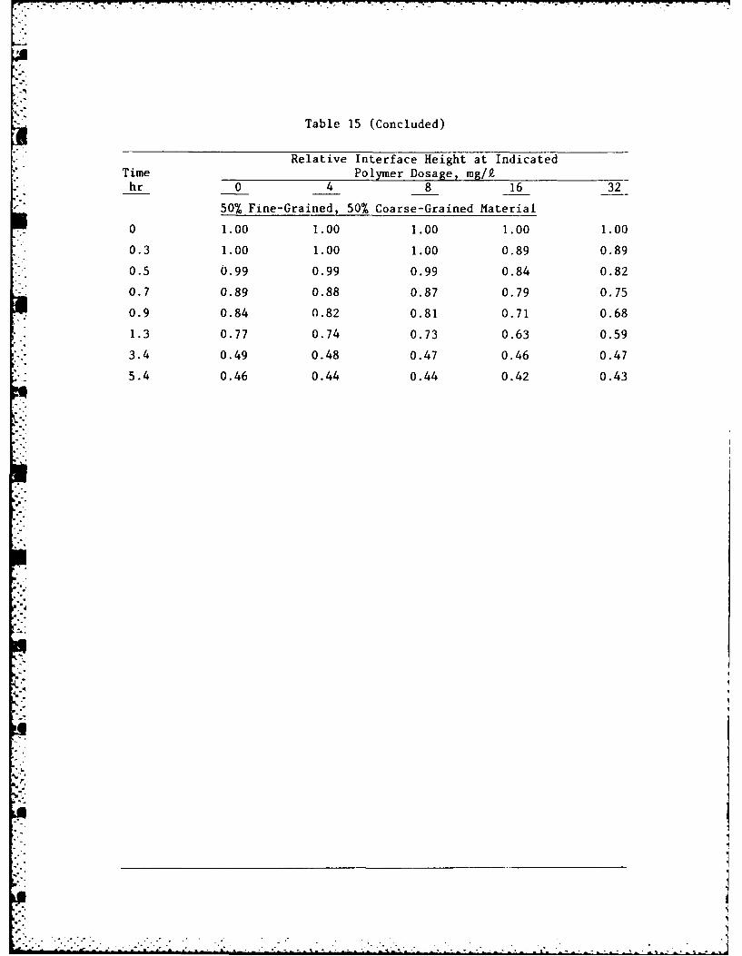
Table 15 (Concluded)
Relative Interface Height at IndicatedTime Polymer Dosage, mg/.ehr 0 4 8 16 32
- 50% Fine-Grained, 50% Coarse-Grained Material
0 1.00 1.00 1.00 1.00 1.00
0.3 1.00 1.00 1.00 0.89 0.89
0.5 0.99 0.99 0.99 0.84 0.82
0.7 0.89 0.88 0.87 0.79 0.75
0.9 0.84 0.82 0.81 0.71 0.68
1.3 0.77 0.74 0.73 0.63 0.59
3.4 0.49 0.48 0.47 0.46 0.47
5.4 0.46 0.44 0.44 0.42 0.43
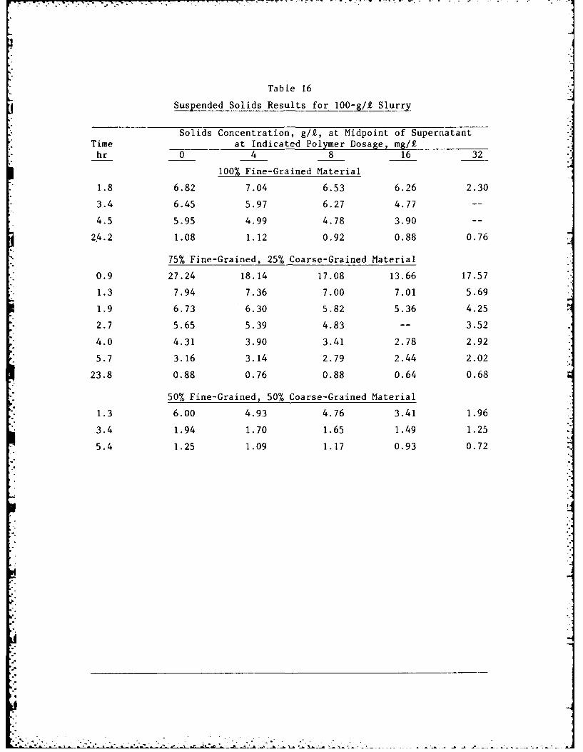
Table 16
Suspended Solids Results for 100-g/2 Slurry
Solids Concentration, g/2, at Midpoint of SupernatantTime at Indicated Polymer Dosage, mg/-hr 0 4 8 16 32
100% Fine-Grained Material
1.8 6.82 7.04 6.53 6.26 2.30
3.4 6.45 5.97 6.27 4.77 --
4.5 5.95 4.99 4.78 3.90 --
24.2 1.08 1.12 0.92 0.88 0.76
75% Fine-Grained, 25% Coarse-Grained Material
0.9 27.24 18.14 17.08 13.66 17.57
1.3 7.94 7.36 7.00 7.01 5.69
1.9 6.73 6.30 5.82 5.36 4.25
2.7 5.65 5.39 4.83 -- 3.52
4.0 4.31 3.90 3.41 2.78 2.92
5.7 3.16 3.14 2.79 2.44 2.02
23.8 0.88 0.76 0.88 0.64 0.68
50% Fine-Grained, 50% Coarse-Grained Material
1.3 6.00 4.93 4.76 3.41 1.96
3.4 1.94 1.70 1.65 1.49 1.25
5.4 1.25 1.09 1.17 0.93 0.72
- . - .-.
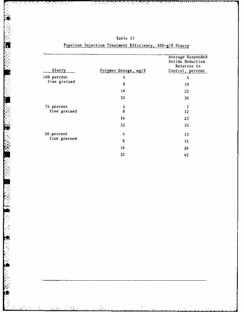
*
Table 17
Pipeline Injection Treatment Efficiency, 100-g/.e Slurry
Average SuspendedSolids Reduction
Relative toSlurry Polymer Dosage, mg/2 Control, percent
100 percent 4 4fine grained 8 10
16 22
32 30
-.- 75 percent 4 7
fine grained 8 12
16 23
32 3350 percent 4 13
fine grained 8 15
16 26
32 42
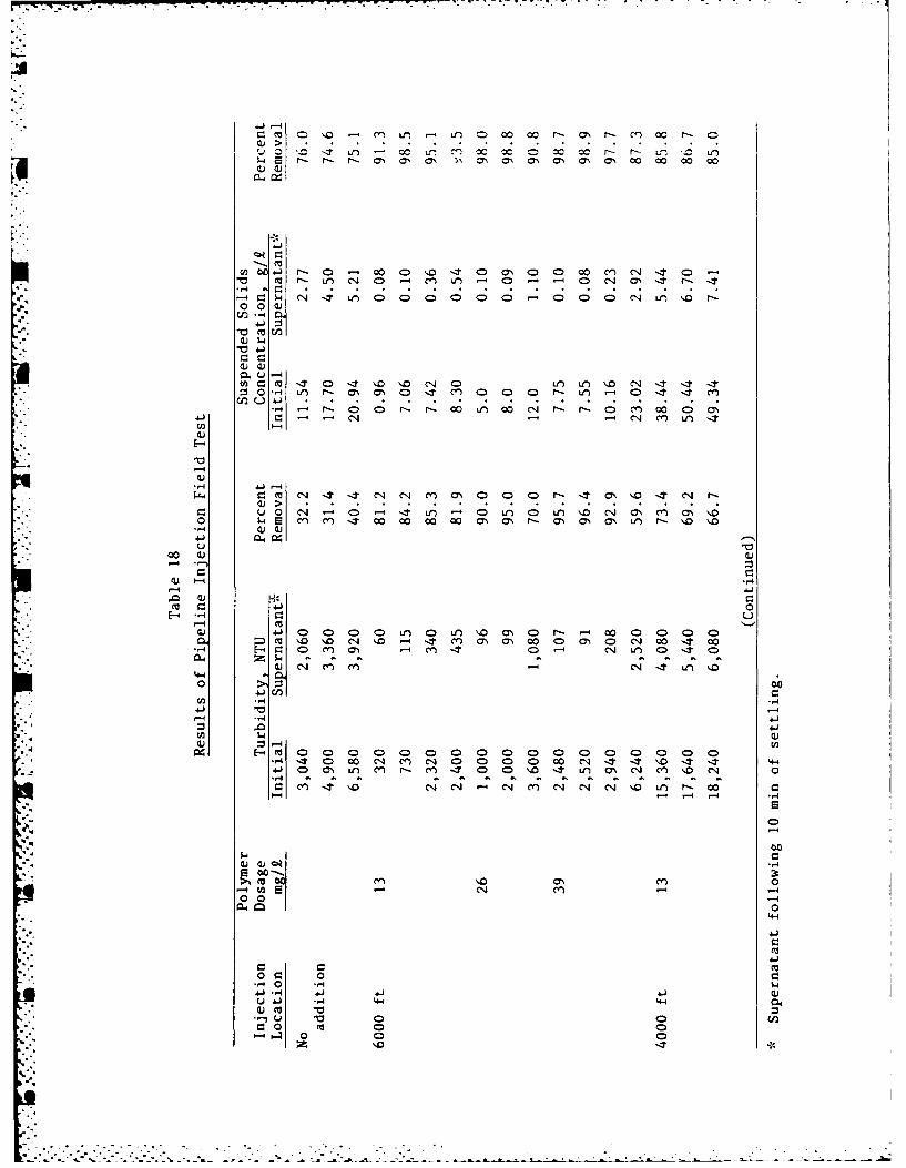
jQ
U)O ,r 0 . 0 0 C) .f - C ) 00000 C 0 t-. a' r- C,4 , C0 - 0LIO N. CD Mn -00 C)~00 0 0 0 t- h.I 0
in. u -4
- . M - 0f 'NJ 10 C' /) 0 r LO 0 1J0 ' C4 -T0- -~4 (nJ .r- ' 0 0 0 0 0 0 0 0 (NT MLrC)C r r 'T0 m
u 0 N4 . . 'T0 Ln 0 (D n ) In \-O N ' m m m.\
0 4 S M I-T W - 00 n 00 '1(3 r- 7N- 0 M n 0- 0 a'04J a4 N (N ~ n .
'00-4V
4-4w 40C :; J M4. (N N '' a 0 - ' '. '04 (J
-4O -4 I - 0 4 L 0 In 0 a1. NJa ~a
-4-)
-4r- Vm0 VDC D0 C c
-44
04W
0 00
~0 0-
0 000 0 0 0 0 0 0 0 0
41 .1 4 ' 4 A.) 4J N N (' N N NJ '0 I -u 4 4 - 4-
tv 10
V VW0C:' 0. m' Q4
0 a 0
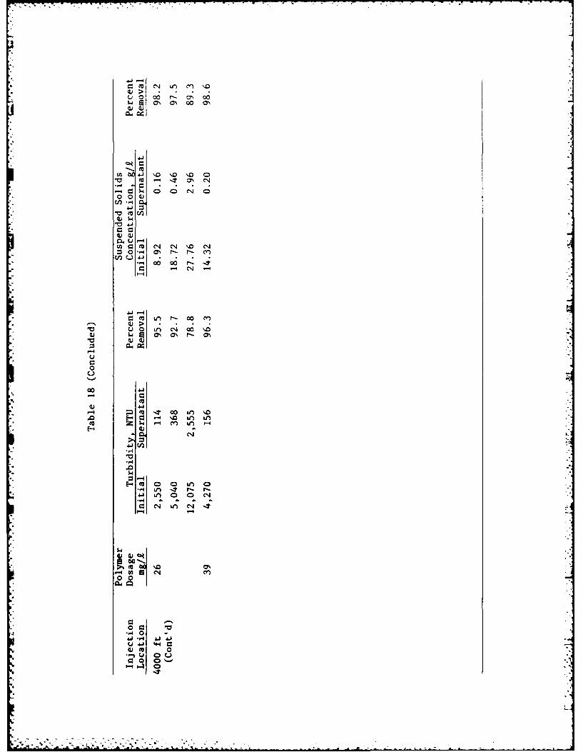
u 0 00 r- all 0
o 0 0
V m
0 1
0 M-S N. .0 'z 0 -- ~C
-4~1 00 C'J
00
m. IT 00 LM 1.0W - c 'J '-
-C4
m0 L) 0 0 '.0a
-- 4
0 0
0
U 0
E-4 0 0 0 r 0
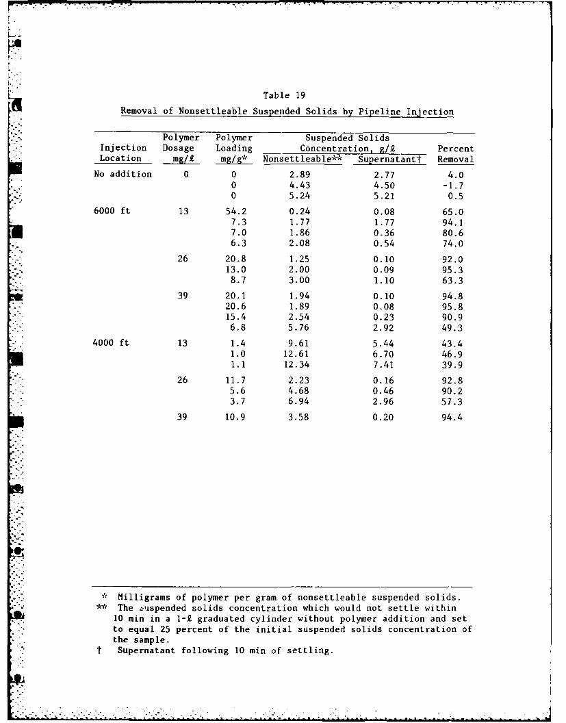
Table 19
Removal of Nonsettleable Suspended Solids by Pipeline Injection
Polymer Polymer Suspended SolidsInjection Dosage Loading Concentration, g/2 Percent
* Location mg/2 mg/g* Nonsettleable** Supernatantf Removal
No addition 0 0 2.89 2.77 4.00 4.43 4.50 -1.70 5.24 5.21 0.5
6000 ft 13 54.2 0.24 0.08 65.07.3 1.77 1.77 94.17.0 1.86 0.36 80.66.3 2.08 0.54 74.0
26 20.8 1.25 0.10 92.013.0 2.00 0.09 95.38.7 3.00 1.10 63.3
39 20.1 1.94 0.10 94.820.6 1.89 0.08 95.815.4 2.54 0.23 90.96.8 5.76 2.92 49.3
4000 ft 13 1.4 9.61 5.44 43.41.0 12.61 6.70 46.91.1 12.34 7.41 39.9
26 11.7 2.23 0.16 92.85.6 4.68 0.46 90.23.7 6.94 2.96 57.3
39 10.9 3.58 0.20 94.4
*Milligrams of polymer per gram of nonsettleable suspended solids.**The 3,!ispended solids concentration which would not settle within10 min in a 1-2 graduated cylinder without polymer addition and setto equal 25 percent of the initial suspended solids concentration ofthe sample.
t Supernatant following 10 min of settling.
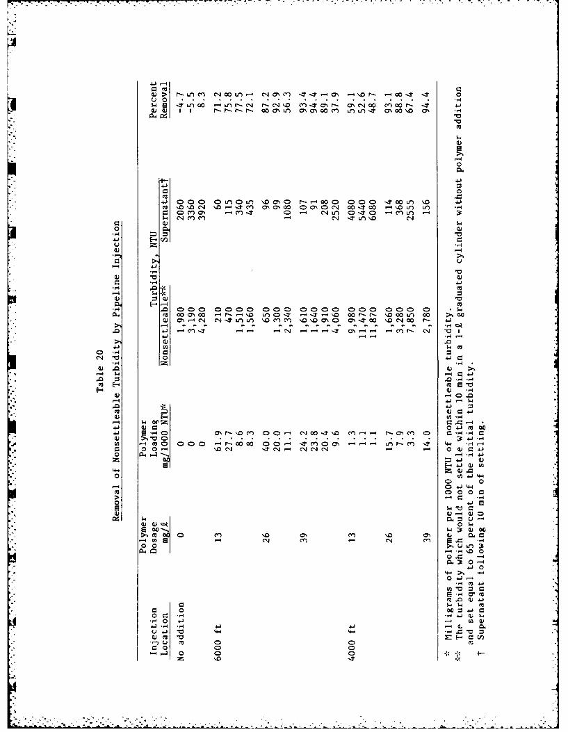
GJ > r- Lt)( Jl N00 Lf)-4 C-.j0'CY -T-ON .-4'.O P- -4o00-It -T 0
0.) 0.) 1 1 rl-r~-r-- r- 00 ON r) CN as0 Y r Lr) -T ONo~ 0\D ON
0
44-
0
4J) 00 (C0Lr0Ln ,DC C0O) r- r 0 000 -00 L) \Qo 4
M \D \)O \ -TY. M Y 0 CD C% QC4 0-.T 0 - \-OLf) V)- -
1.4 C -N CN LfT ) 1 C J LO 4
U(0)-
4-1 E4)n
-44-
-41-.. ...
10 Q- Q C -4 C) 0 C) C 0 C)~r a C'CJC 0 CDCID DCG)C44.S TV) L-\ D %C N-4 40 \OC* 0 P .41
0.T r.N-04 T ONC)r N "0 4-)
C) .0:)3
-4 w- -4 ~4-).0 Z 'a*- -
4) r-40 .0
.0 4-)1
0) 4E-~0-4) w74 w-0C 00-0.~C -~~0 d 4 -01 4) C:041m04J .4 J a ONr .C) 4 C 0 T\o.Y -CNC 4-
1~ 0 000 3~~0 'L~~C 4 L.4 4. 4
0 0 \.O cJ -I .dC14 N.JC14c -4 0 (U r.
4-41
0 U ) 4 -10 0a- 4-J 4-4
>~ .'-4
00 a~a) 0) -q a)0
0) 0s00 00 ' ' ~ '00
I-4 cn CNCY C40Y
-4~ -4-4
41 0
0
C .14 m 4-1
C3 0 00 Z 41 C0 C: -4~ 0 -r 0 4.1U0
j... 10 4.4 4-4 -0. =
0 0c000
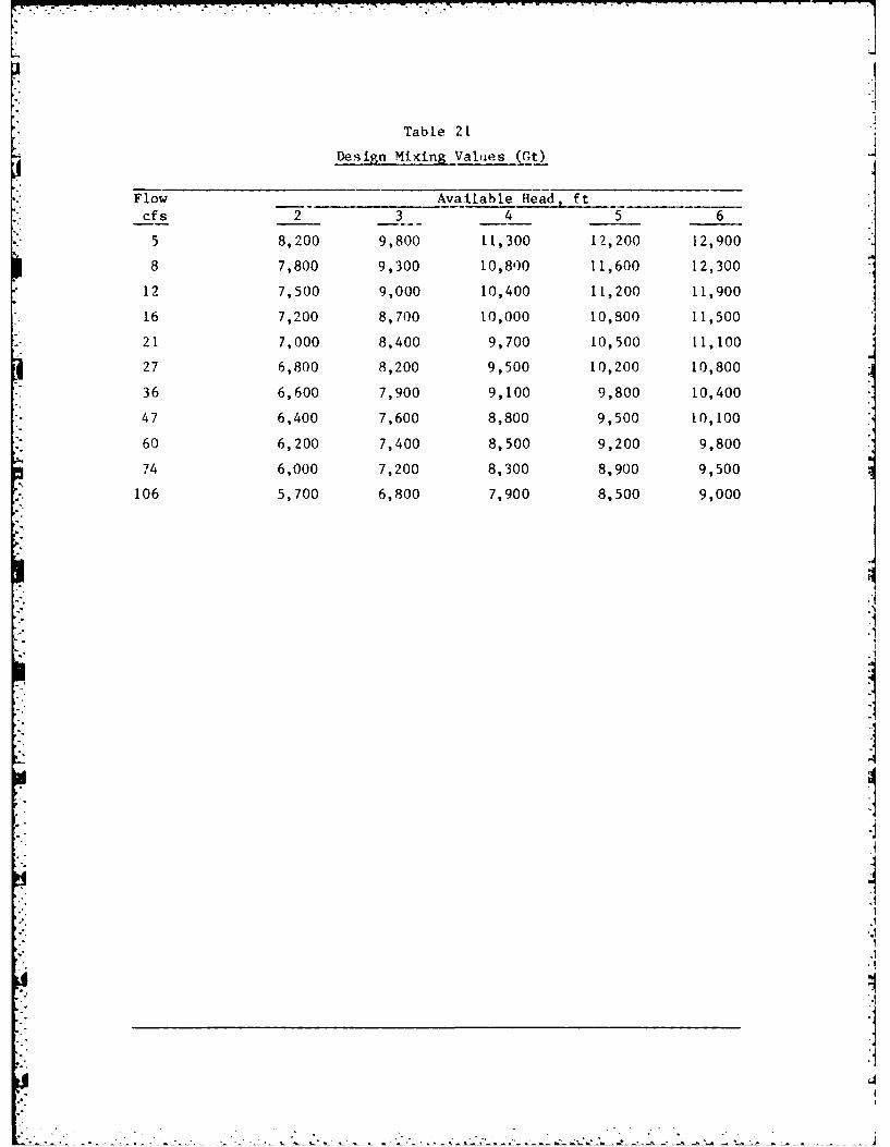
Table 21
Design Mixing Values (Gt)
Flow Available Head, ftcfs 2 3 4 5 6
5 8,200 9,800 11,300 12,200 12,900
8 7,800 9,300 10,800 11,600 12,300
12 7,500 9,000 10,400 11,200 11,900
16 7,200 8,700 10,000 10,800 11,500
21 7,000 8,400 9,700 10,500 11,100
27 6,800 8,200 9,500 10,200 10,800
36 6,600 7,900 9,100 9,800 10,400
47 6,400 7,600 8,800 9,500 10,100
60 6,200 7,400 8,500 9,200 9,800
74 6,000 7,200 8,300 8,900 9,500
106 5,700 6,800 7,900 8,500 9,000
.'1
I
.1
.I>1
' 4 " 1 " ' ft i . ' - . - t. , .- 1 - '"' , "- ' " '' . " '
-1.4 4
.... .. . y"" " :t- ' .... . .
A 41 -4: La
p6. iikFSi.
S ,. f i I.K5, ' • § j .] *... ," ' 'V' .. " '--
-~, . A Ai" . A - . ..
,4.- .4... . ., , ..S .. ..r.,.. .... . .
::i" f -"% " " < '* d . . " "" "' .'' .' "
r 4t . 4 . .
I999"999 N 1
..
"'4
4, *'. , .f.".' ! ., i . / ..
i
4kA" ...
.:' . <9~~ 9- ..,r.
t "g.."4 ..... ... .. A "' ->... 4
. .. ....4 :'. 4 1" ...
a" - " a • 4 - : : " .
t": , , '
A• . .. !r V < ., , ,. ir, atis.&. , 4 ' i *,
,W I: . , / ... *,. . .U'
' " ." -" -S . .....
4 , :t i ( '- ''t, .,""


![SMART CITY NR ONRENE REORT When Chandigarh Mulled Smart ...€¦ · SMART CITY NR ONRENE REORT 38 NOVEMBER 2018 [ egov.eletsonline.com ] The Largest Portal on e-Governance in Asia](https://img.pdfslide.us/doc/110x75/5f072f237e708231d41bb99b/smart-city-nr-onrene-reort-when-chandigarh-mulled-smart-smart-city-nr-onrene.jpg)