ICES REPORT 16-04

February 2016

Pressure and fluid-driven fracture propagation in porousmedia using an adaptive finite element phase field model

by

Sanghyun Lee, Mary F. Wheeler, Thomas Wick

The Institute for Computational Engineering and SciencesThe University of Texas at AustinAustin, Texas 78712

Reference: Sanghyun Lee, Mary F. Wheeler, Thomas Wick, "Pressure and fluid-driven fracture propagation inporous media using an adaptive finite element phase field model," ICES REPORT 16-04, The Institute forComputational Engineering and Sciences, The University of Texas at Austin, February 2016.

Pressure and fluid-driven fracture propagation inporous media using an adaptive finite element

phase field model

Sanghyun Lee ∗ Mary F. Wheeler † Thomas Wick ‡

This work presents phase field fracture modeling in heterogeneous porous media. Wedevelop robust and efficient numerical algorithms for pressure-driven and fluid-driven set-tings in which the focus relies on mesh adaptivity in order to save computational cost forlarge-scale 3D applications. In the fluid-driven framework, we solve for three unknownspressure, displacements and phase-field that are treated with a fixed-stress iteration inwhich the pressure and the displacement-phase-field system are decoupled. The latter sub-system is solved with a combined Newton approach employing a primal-dual active setmethod in order to account for crack irreversibility. Numerical examples for pressurizedfractures and fluid filled fracture propagation in heterogeneous porous media demonstrateour developments. In particular, mesh refinement allows us to perform systematic studieswith respect to the spatial discretization parameter.

Keywords: Phase Field; Fluid Filled Fracture; Adaptive Finite Elements; Porous Media; Primal-Dual Active Set

1 Introduction

Crack propagation in brittle and porous media is currently one of the major research topics in me-chanical, energy, and environmental engineering. In this paper, we concentrate specifically on frac-ture propagation in three dimensional heterogeneous porous media. We consider a variational ap-proach for brittle fracture introduced by Francfort and Marigo [18] that is formulated in terms ofa thermodynamically-consistent phase field technique; see Miehe et al. [32]. Other approaches fortreating pressurized fracture include the following: cohesive zone finite elements (CZ-FEM) [17],displacement discontinuity methods (DDM) [40, 44, 56], partition-of-unity methods and closely re-lated XFEM/GFEM (extended and generalized finite elements) methods [21, 22, 23, 29, 45, 46, 50].Boundary element methods have been employed in [15, 19], and peridynamics for hydraulic fractur-ing has been considered in [27]. Discrete networks of fluid filled fractures have been investigated in[8, 28, 30, 39, 47].

∗Center for Subsurface Modeling, The Institute for Computational Engineering and Sciences, The University of Texasat Austin, Austin, Texas 78712, USA

†Center for Subsurface Modeling, The Institute for Computational Engineering and Sciences, The University of Texasat Austin, Austin, Texas 78712, USA

‡RICAM, Austrian Academy of Sciences Altenberger Str. 69 4040 Linz, Austria

1

Our motivations for employing a phase field model are that fracture nucleation, propagation, kinking,and curvilinear paths are automatically included in the model; post-processing of stress intensityfactors and remeshing resolving the crack path are avoided. Furthermore, the underlying equations arebased on continuum mechanics principles that can be treated with adaptive Galerkin finite elements. Infact, variational and phase field formulations for fracture are active research areas as attested in recentyears; see Bourdin et al. [10, 11], Miehe et al. [31, 32, 33], Borden et al. [9], Artina et al. [6], Burke et al.[14], Allaire et al. [1], Schluter et al. [48], Ambati et al. [2], Mikelic et al. [36, 38]. Here, discontinuitiesin the displacement field across the lower-dimensional crack surface are approximated by an auxiliaryphase field function. The latter can be viewed as an indicator function, which introduces a diffusivetransition zone between the broken and the unbroken material.

For pressurized fractures in porous media, the pressure is a fixed, given quantity or assumed tobe computed [38, 52]. The essential aspects of a phase field-based pressurized-fracture propagationformulation are techniques that must include resolution of the length-scale parameter ε, the numericalsolution of the forward problem and enforcement of the irreversibility of crack growth. The sum ofthese requirements leads to a variational inequality. For numerical simulations, a robust computationalframework in terms of a quasi-monolithic formulation has been proposed in [24] in which a primal-dualactive set method (i.e., a semi-smooth Newton method [26]) is coupled with the Newton solver for thenonlinear forward problem.

Our main attention in this paper is on three-dimensional applications that are challenging becauseof computational cost. This is especially the case for phase-field problems because the resolutionof the crack requires (very) fine meshes. Here, uniform refinement is infeasible and we adopt amethod proposed in [24] for two-dimensional problems and extend these ideas to three-dimensionalapplications. The efficiency is shown in terms of pressurized and fluid-filled phase-field fractures forwhich systematic 3D studies including mesh refinements are not present in the literature.

In summary, the goal and novelty of the present paper are systematic studies of computationalstability using predictor-corrector mesh adaptivity for three-dimensional pressure and fluid-drivenphase-field fracture problems. Such studies are essential for better understanding between modeland discretization parameters in phase-field modeling for the previously mentioned applications. Weemphasize that the fluid-filled fracture framework in porous media (with Biot’s coefficient α = 1) isitself novel where we formulate a fixed-stress iteration for the pressure system coupled to the fully-coupled displacement-phase-field system. Here, the latter system is treated with a primal-dual activeset method. This idea is in contrast to the fluid-filled phase-field fracture framework presented in [37]in which all equations have been decoupled.

The outline of this paper is as follows: We first state the governing equations in Section 2. Then,we present our main algorithm and adaptive discretization in Section 3. In Section 4, we providenumerical examples that demonstrate the potential of this approach for treating practical engineeringapplications.

2 Mathematical Models for Pressurized and Fluid Filled Fractures

Let Λ ∈ Rd, d = 2, 3 be a smooth open and bounded computational domain with Lipschitz boundary∂Λ and let [0, T ] be the computational time interval, T > 0. We assume that the crack C is containedcompactly in Λ. Here, we emphasize that the crack is seen as a thin three-dimensional volume wherethe thickness is much larger than the pore size of the porous medium. The displacement of thesolid and diffusive flow in the porous medium are modeled in Ω = Λ\C by the classical quasi-staticelliptic-parabolic Biot system for a linear elastic, homogeneous, isotropic, porous solid saturated witha slightly compressible viscous fluid for every t ∈ (0, T ].

2

First, we start from the constitutive equation for the Cauchy stress tensor σpor,

σpor(u, p)− σ0 = σ(u)− α(p− p0)I, in Ω× (0, T ] (1)

where u : Ω× [0, T ]→ Rd is the solid’s displacement, p : Ω× [0, T ]→ R is the fluid pressure, α ∈ [0, 1]is the Biot coefficient, I is the identity tensor, σ0 and p0 are the given initial values when t = 0, whichare set to be zero for simplicity in this paper. The effective linear elastic stress tensor σ := σ(u) is

σ(u) = λ(∇ · u)I + 2Ge(u), (2)

where λ,G > 0 are the Lame coefficients. The linear elastic strain tensor is given as

e(u) =∇u +∇uT

2. (3)

Then the balance of linear momentum in the solid reads

−∇ · σpor(u, p) = ρsg in Ω× (0, T ], (4)

where ρs is the density of the solid and g is the gravity. Next, the flow pressure equation is given by

∂t(ρFϕ?) +∇ · (ρFv) = q in Ω× (0, T ] (5)

where

ϕ? = ϕ?0 + α∇ · u +1

M(p− p0) (6)

is fluid volume fraction with ϕ?0 initial value, ρf fluid density, q is the source/sink term, and Biotmodulus M > 0. The velocity is defined by Darcy law,

v = −Kη

(∇p− ρFg) in Ω× (0, T ], (7)

where η is the fluid viscosity, ρF is the fluid density, and K is the permeability.

2.1 The Phase Field Energy Functional for Pressurized Fractures

Based on the linear momentum in the solid (4), we introduce the Francfort-Marigo functional [18],which describes the energy of a crack in an elastic medium as

E(u, C) =1

2

∫Ωσ(u) : e(u) +GcH

d−1(C) dx. (8)

The Hausdorff measure Hd−1(C) denotes the length of the crack and is multiplied by a materialproperty Gc > 0, that is considered in fracture mechanics to be the critical energy release rate. Weconsider the pressure energy by adding an additional pressure term in (1) as derived in [38, 36]. Thuswe can rewrite (8) by

E(u, p, C) =1

2

∫Ωσ(u) : e(u) dx−

∫Ωαp∇ · u dx +GcH

d−1(C). (9)

We introduce the continuous phase field variable ϕ : Λ × [0, T ] → [0, 1] where ϕ(x, t) = 0 in thecrack region and ϕ(x, t) = 1 in the unbroken material. This introduces a diffusive transition zone,which is controlled by the regularization parameter ε > 0; see Figure 1 for details.

3

(a)

ε

ϕ = 0ϕ ∈ (0, 1)

ϕ = 1

(b)

Figure 1: Fracture representation using the phase field ϕ. (a) The inner blue region indicates thecrack with ϕ = 0 and the outer red region indicates the unbroken zone where ϕ = 1. Wehave the linear diffusive transition zone near the interface of the fracture (green region). (b)Illustrates the transition zone with the thickness ε.

Before, we can write the full energy functional, we must model the interaction of fracture (pF ) andreservoir (pR) pressures. This is modeled as an interface law. We assume that the fracture length (orsurface area) is much larger than its width (or aperture). Therefore a lubrication approximation ofthe stress at the interface C is a plausible choice. The fracture pressure pF is in equilibrium with thenormal component of reservoir stress at the crack C such that,

σporn = (σ(u)− αpRI)n = −pFn, (10)

where n is the normal unit vector. Further assuming pressure continuity at C the pressure field p issuch that p = pF on C and p = pR in Λ\C. The fracture pressure contribution is reflected in thesurface force integral, second term in the right hand side of the functional (9) over C as:∫

Cτu dS =

∫Cσpornu dS = −

∫Cpun dS = −

∫Ω∇ · (pu) dx +

∫∂Λpun dS

= −∫

Ω(u · ∇p+ p∇ · u) dx +

∫∂Λpun dS, (11)

resulting in a volumetric representation for the pressure. We assume Dirichlet boundary conditionsfor pressure on ∂Λ, and therefore the last term in (11) vanishes. Thus we have∫

Cτu dS = −

∫Λ

(u · ∇p+ p∇ · u) dx.

We consider the global constitutive dissipation functional of Ambrosio-Tortorelli type [3, 4], for a rateindependent fracture process. This means, we extend all integrals from C and Ω to Λ. For the elasticenergy terms this has been often explained in the literature. For the pressure terms we follow [38]:

−∫

Ω(u · ∇p+ p∇ · u) dx → −

∫Λϕ2(u · ∇p+ p∇ · u) dx.

Then, we obtain

Eε(u, p, ϕ) =

∫Λ

1

2((1− k)ϕ2 + k)σ+(u) : e(u) dx+

∫Λ

1

2σ−(u) : e(u) dx−

∫Λ

(α− 1)ϕ2p∇ · u dx

+

∫Λ

(ϕ2∇p)u dx +Gc

∫Λ

(1

2ε(1− ϕ)2 +

ε

2(∇ϕ)2

)dx. (12)

4

Here ε is the thickness of the diffusive zone shown in Figure 1b and k is a small regularizationparameter, k ε. Regarding the stress tensor split, we follow Amor et al. [5] (see also Borden et al.[9], p. 79, for a brief discussion on the differences between different models). The stress tensor isadditively decomposed into a tensile part σ+(u) and a compressive part σ−(u) by:

σ+(u) := (2

dG+ λ)tr+(e(u))I + 2G(e(u)− 1

dtr(e(u))I), (13)

σ−(u) := (2

dG+ λ)tr−(e(u))I, (14)

where

tr+(e(u)) = max(tr(e(u)), 0), and tr−(e(u)) = tr(e(u))− tr+(e(u)). (15)

We emphasize that the energy degradation only acts on the tensile part. Finally, we assume that crackgrowth is irreversible. Here we follow [31, 32] and formulate the irreversibility condition as

∂tϕ ≤ 0. (16)

The resulting system is a variational inequality that has been mathematically analyzed by Mikelicet al. [38].

2.2 Pressure Diffraction Equation for Modeling Fluid Filled Fractures

In order to formulate the flow equations in the porous media zone and the fracture, respectively, weemploy the phase field function as an indicator function. Thus, the flow pressure equations (5)-(6)can be separated for the fracture and the reservoir sub-domain respectively.

We denote by ΩF (t) and ΩR(t) the open subsets of the space-time domain Λ × [0, T ] at time t.ΩR(t) is filled with the unbroken material (reservoir domain). In the approximation, the fracture isapproximated by a volume term and C becomes ΩF (t). Thus, we define ∂C := Γ(t) := ΩF (t) ∩ ΩR(t).

To derive the flow pressure equations for each sub-domain, first we consider the two separate masscontinuity equations for the fluid in the reservoir and the fracture from (5), which we can rewrite as

∂t(ρFϕ?F ) +∇ · (ρFvF ) = qF − qL in ΩF × (0, T ], (17)

∂t(ρRϕ?R) +∇ · (ρRvR) = qR in ΩR × (0, T ]. (18)

Here ϕ?R and ϕ?F are the reservoir and fracture fluid fraction respectively and we assume ϕ?F = 1 (sincethe porosity of the fracture is one). Recall the reservoir fluid fraction is given in (6). In addition, theleak-off term qL is defined in (31), and qF and qR are source/sink terms for fracture and reservoir,respectively.

Next, we describe the flow given by Darcy’s law at (7) for the fracture (j = F ) and for the reservoir(j = R), respectively by

vj = −Kj

ηj(∇pj − ρjg). (19)

We assume the fluid in the reservoir and the fracture is slightly compressible, thus we define the fluiddensity as

ρj := ρ0j exp(cj(pj − p0

j )) ≈ ρ0j [1 + cj(pj − p0

j )], (20)

where ρ0j is the reference density and cj is the fluid compressibility.

5

Following the general reservoir approximation with the assumption that cR and cF are small enough,we use ρR = ρ0

R and ρF = ρ0F to rewrite the equations (17)-(18) by

ρ0R∂t(

1

MpR + α∇ · u)−∇ ·

KRρ0R

ηR(∇pR − ρ0

Rg) = qR in ΩR × (0, T ], (21)

ρ0F cF∂tpF −∇ ·

KFρ0F

ηF(∇pF − ρ0

Fg) = qF − qL in ΩF × (0, T ]. (22)

For the fracture flow, we adopt a three-dimensional lubrication equation [37]. Inside this function,the fracture permeability is assumed to be isotropic such that

KF =1

12w(u)2,

where w(u) = [u · n] denotes the aperture (width) of the fracture, which means that the jump [·] ofnormal displacements has to be computed. For calculating the aperture we apply an integral formusing the phase field variable; details can be found in [51], p.51. Furthermore, we use an interpolatedpermeability K in the phase field transition zone, eg. K = ϕKR + (1 − ϕ)KF . For ϕ = 1 (in thereservoir), we have KR and in the fracture ϕ = 0, we have KF ; see Section 3.1 for more details.

2.3 Initial and Boundary Conditions

The system is supplemented with initial and boundary conditions. The initial condition for the pressurediffraction equations (21)-(22) is given by pF (x, 0) = p0

F for all x ∈ ΩF (t = 0) and pR(x, 0) = p0R for

all x ∈ ΩR(t = 0), where p0F and p0

R are smooth given pressures. Also we have ϕ(x, 0) = ϕ0 for allx ∈ Λ(t = 0), where ϕ0 is a given smooth initial fracture.

For u we prescribe Dirichlet boundary conditions on ∂Λ. Specifically, given fu : ∂Λ → Rd andfp : ∂ΛD → R, we require that

u = fu on ∂Λ× (0, T ], (23)

p = fp on ∂ΛD × (0, T ], (24)

KR(∇pR − ρ0Rg) · n = 0 on ∂ΛN × (0, T ], (25)

[p] = 0 on Γ× (0, T ], (26)

KR

µR(∇pR − ρ0

Rg) · n =KF

µF(∇pF − ρ0

Fg) · n on Γ× (0, T ], (27)

where n is the outward pointing unit normal on Γ or ∂ΛN . The pressure boundary ∂Λ is decomposedinto two non-overlapping components ∂Λ = ∂ΛD ∪ ∂ΛN with ∂ΛN ∩ ∂ΛD = ∅. For the phase fieldfunction, we prescribe homogeneous Neumann conditions on ∂Λ as it is usually done.

3 Numerical Methods, Algorithms and Discretization

We consider a mesh family Thh>0, which is assumed to be shape regular in the sense of Ciarlet, andwe assume that each mesh Th is a subdivision of Λ made of disjoint elements K, i.e., squares whend = 2 or cubes when d = 3. Each subdivision is assumed to exactly approximate the computationaldomain, thus Λ = ∪K∈ThK. The diameter of an element K ∈ Th is denoted by h and we denote hmin

for the minimum. For any integer k ≥ 1 and any K ∈ Th, we denote by Qk(K) the space of scalar-valued multivariate polynomials over K of partial degree of at most k. The vector-valued counterpartof Qk(K) is denoted QQQk(K). We define a partition of the time interval 0 =: t0 < t1 < · · · < tN := Tand denote the time step size by δt := tn − tn−1.

6

0.5ϕ

c1 c20

1 χR

χF

1

(a)

ε

ϕ = 0

ϕ = 1

c1

c2

(b)

Figure 2: (a) The linear indicator functions χF and χR illustrated with adjustable constants c1 andc2. (b) We consider as the fracture zone if ϕ ≤ c1 and as the reservoir zone if ϕ ≥ c2

3.1 Decomposing the Domain into ΩF and ΩR, Leakage Term, and Well Model

In this section, we define the fracture domain ΩF and the reservoir domain ΩR by introducing twolinear indicator functions χF and χR for the two different sub-domains; they satisfy

χR(·, ϕ) := χR(x, t, ϕ) = 1 in ΩR(t), and χR(·, ϕ) = 0 in ΩF (t), (28)

χF (·, ϕ) := χF (x, t, ϕ) = 1 in ΩF (t), and χF (·, ϕ) = 0 in ΩR(t). (29)

Thus χF (·, ϕ) is zero in the reservoir domain and χR(·, ϕ) is zero in the fracture domain. In thediffusive zone, the linear functions are defined as

χF (·, ϕ) = − (ϕ− c2)

(c2 − c1)and χR(·, ϕ) =

(ϕ− c1)

(c2 − c1). (30)

Thus χR(·, ϕ) = 0 and χF (·, ϕ) = 1 if ϕ(x, t) ≤ c1, and χR(·, ϕ) = 1 and χF (·, ϕ) = 0 if ϕ(x, t) ≥ c2,where c1 := 0.5− cx and c2 = 0.5 + cx. For simplicity we set cx = 0.1, and refer the reader to Figure2 for more details.

We define the leak-off term asqL := ∇ · (ρFvleak) (31)

and the effective velocity for the fracture by

vF = −KF

ηF(∇pF − ρFg) + vleak. (32)

In particular, the gravity term g? is re-scaled and implicitly contains the leakage term. i.e., g? :=χR(·, ϕ)g + χF (·, ϕ)(g + (K−1

eff/ρ0F )vleak), where Keff := χF (·, ϕ)KF + χR(·, ϕ)KR including interpo-

lation of KF and KR in the phase field transition zone [37].The well terms qR and qF in (21)-(22) are described by suitable well models. Following Peaceman’s

model [16, 42, 43], we define the source term as,

qF := CQj (pb − p)×H(x), qR := −CQj (pb − p)×H(x), CQj :=2πρi√k11k22h3

µi ln (re/rw), j = F,R, (33)

where re is the outer equivalent radius, rw is the inner radius, and h3 is the thickness of the well bore.pb is a given well bore pressure and we have given anisotropic permeability K = diag(k11, k22, k33).Here H(x) is defined as

H(x) :=

1 if |x−X| ≤ c.0 otherwise,

(34)

where c is a sufficiently small positive constant, and X is a given source/sink point in the domain.

7

3.2 Discretization of the Pressure Diffraction Equation

First, we discuss temporal discretization of the pressure diffraction equations (21)-(22) and afterwardstheir spatial treatment.

3.2.1 Approximation in Space

The space approximation P of the pressure function p(x, t) is approximated by using continuouspiecewise polynomials given in the finite element space,

W(T ) := W ∈ C0(Λ;R) | W |K ∈ Q1(K),∀K ∈ T . (35)

Assuming that the displacement field and the phase field is known, the Galerkin approximation of(21)-(22) is formulated as follows. Given P (x, 0) = P 0 where P 0 is an approximation of the initialcondition p0, find P ∈ C1([0, T ];W(T )) such that

χR(·, ϕ)

(∫Λρ0R∂t(

1

MP + α∇ · u)ω dx +

∫Λ

KRρ0R

ηR(∇P − ρ0

Rg)∇ω dx =

∫ΛqRω dx

), ∀ω ∈W(T ),

(36)

χF (·, ϕ)

(∫Λρ0F cF∂tPω dx +

∫Λ

KFρ0F

ηF(∇P − ρ0

Fg)∇ω dx =

∫Λ

(qF − qL)ω dx

), ∀ω ∈W(T ). (37)

3.2.2 Approximation in Time

We denote the approximation of P (x, tn), 0 ≤ n ≤ N by Pn, and assume u(tn+1) and ϕ(tn+1) are givenvalues at time tn+1. Then, the time stepping proceeds as follows: Given Pn, compute Pn+1 ∈W(T )so that

BR(Pn+1)(ω) := χR(·, ϕ(tn+1))

(∫Λρ0R

( 1

M

(Pn+1 − Pn

δt

)+ α

(∇ · un+1 −∇ · un

δt

))ω dx

+

∫Λ

KRρ0R

ηR(∇Pn+1 − ρ0

Rg)∇ω dx−∫

ΛqRω dx

)∀ω ∈W(T ) (38)

BF (Pn+1)(ω) := χF (·, ϕ(tn+1))

(∫Λρ0F cF

(Pn+1 − Pn

δt

)ω dx +

∫Λ

KFρ0F

ηF(∇Pn+1 − ρ0

Fg)∇ω dx

−∫

Λ(qF − qL)ω dx

), ∀ω ∈W(T ) (39)

Formulation 1. Find Pn+1 ∈W(T ) for all times tn+1 such that

B(Pn+1)(ω) = BR(Pn+1)(ω) +BF (Pn+1)(ω) = 0 ∀ω ∈W(T ). (40)

8

3.3 A Fully-Coupled Formulation of the Euler-Lagrange Equations for u and ϕ

In this section, we present a fully-coupled Euler-Lagrange formulation for U and Φ (approximat-ing u, ϕ), respectively. We consider a time-discretized system in which time enters through theirreversibility condition. The spatial discretized solution variables are U ∈ C1([0, T ];VVV0(T )) andΦ ∈ C1([0, T ];Z(T )), where

VVV0(T ) := W ∈ C0(Λ;Rd) | W = 0 on ∂Λ,W |K ∈QQQ1(K),∀K ∈ T , (41)

Z(T ) := Z ∈ C0(Λ;R)| Zn+1 ≤ Zn ≤ 1, Z|K ∈ Q1(K), ∀K ∈ T . (42)

Moreover, we extrapolate Φ (denoted by E(Φ)) in the first terms (i.e., the displacement equation)in Formulation 2 in order to avoid an indefinite Hessian matrix:

E(Φ) = Φn−2 +(t− tn−1 − tn−2)

(t− tn−1)− (t− tn−1 − tn−2)(Φn−1 − Φn−2).

This heuristic procedure has been shown to be an efficient and robust method as discussed in [24].

In the following, we denote by Un,Φn the approximation of U(tn),Φ(tn) respectively.

Formulation 2. Let us assume that Pn+1 is a given approximated pressure at the time tn+1. Giventhe initial conditions U0 := U(0) and Φ0 := Φ(0) we seek Un+1,Φn+1 ∈ VVV0(T )× Z(T ) such that

A(Un+1,Φn+1)(w, ψ−Φn+1) =

∫Λ

(1−k)(E(Φn+1)2+k)σ+(Un+1) : e(w) dx+

∫Λσ−(Un+1) : e(w) dx

−∫

Λ(α− 1)E(Φn+1)2Pn+1∇ ·w dx +

∫ΛE(Φn+1)2∇Pn+1 ·w dx

+ (1− k)

∫Λ

Φn+1σ+(Un+1) : e(Un+1) · (ψ − Φn+1) dx

− 2(α− 1)

∫Λ

Φn+1Pn+1∇ ·Un+1 · (ψ − Φn+1) dx+

∫Λ

2Φn+1∇Pn+1 ·Un+1 · (ψ − Φn+1) dx

−Gc∫

Λ

1

ε(1−Φn+1)·(ψ−Φn+1) dx+Gc

∫Λε∇Φn+1 ·∇(ψ−Φn+1) dx ≥ 0, ∀w, ψ ∈ VVV0(T )×Z(T ).

(43)

This nonlinear variational inequality is solved by combining two Newton methods into one New-ton iteration. The first Newton iteration is necessary for solving the nonlinear forward problemA(Un+1,Φn+1)(w, ψ) = 0. The second iteration is from the constraint Φn+1 ≤ Φn that is realizedvia a semi-smooth Newton method that is equivalent to a primal-dual active set strategy. Furtherdetails are presented below in Section 3.5 and Algorithm 2.

Remark 1 (Further remarks on time-dependencies). The full system is time-dependent although notall equations contain time derivatives. The pressure equation has a time derivative whereas ‘time’in the phase field equation enters through the irreversibility constraint. The displacement solutionchanges in time since the time-dependent variables of the other two equations enter.

Remark 2 (Directional derivative). For later purposes of solving the nonlinear Formulation 2, wecompute the Jacobian that is build by computing the directional derivative A′(Un+1,Φn+1)(δUn+1, δΦn+1,w, ψ).

9

Then find δUn+1, δΦn+1 ∈ VVV0(T )× Z(T ) such that

A′(Un+1,Φn+1)(δUn+1, δΦn+1,w, ψ − Φn+1) =

∫Λ

((1− k)E(Φn+1)2 + k)σ+(δUn+1) : e(w) dx

+

∫Λσ−(δUn+1) : e(w) dx

+(1−k)

∫ΛδΦn+1σ+(Un+1) : e(Un+1) ·(ψ−Φn+1) dx+(1−k)

∫Λ

2Φn+1σ+(δU) : e(U) ·(ψ−Φn+1) dx

− 2(α− 1)Pn+1

∫Λ

(δΦn+1∇ ·Un+1 + Φn+1∇ · δUn+1 · (ψ − Φn+1)) dx

+ 2

∫ΛδΦn+1∇Pn+1 ·Un+1 · (ψ − Φn+1) dx + 2

∫Λ

Φn+1∇Pn+1 · δUn+1 · (ψ − Φn+1) dx

+Gc

∫Λ

1

εδΦn+1 · (ψ − Φn+1) dx +Gc

∫Λε∇δΦn+1 · ∇ψ dx ≥ 0, ∀w, ψ ∈ VVV0(T )× Z(T ). (44)

3.4 The Fixed Stress Split Iterative Method

3.4.1 Basics

The fixed-stress split iterative method is a standard approach in petroleum engineering for decouplinggeomechanics and (multiphase) flow in porous media. The fixed stress split iterative method consistsof imposing constant volumetric mean total stress. This means that the stress

σv = σv,0 +Kdr∇ · (u− u0)− α(p− p0), (45)

is kept constant at the half-time step. Here the fixed stress coefficient is Kdr = 3λ+2µ3 . The iterative

process reads as follows: for l = 0, 1, 2, · · · ,(1

M+

α2

Kdr

)∂tp

l+1 +∇ ·(K

η(ρFg −∇pl+1)

)= − α

Kdr∂tσ

lv + f

= f−α∇ · ∂tul +α2

Kdr∂tp

l (46)

−∇ · σpor(ul+1)+α(∇pl+1) = 0 (47)

until it meets the convergence criteria. As stopping criteria, we either use simply max‖ul−ul−1‖L2(Λ), ‖pl−pl−1‖L2(Λ) ≤ TOLFS or take the residual with respect to the porosity, e.g. [35].

3.4.2 Fixed-Stress Algorithm for the Discretized Fluid Filled Fracture System

As previously explained, we first solve for the pressure, which is in the case of fractures realized as apressure diffraction problem:

Formulation 3. For each time tn+1 we iterate for l = 0, 1, 2, 3, . . . to find P l+1 ∈W such that

[B(Pn+1)(ω)]l+1 = [BR(Pn+1)(ω)]l+1 + [BF (Pn+1)(ω)]l+1 = 0 ∀ω ∈W(T ),

where

[BR(Pn+1)(ω)]l+1 := χR(Φl+1)

(∫Λρ0R

( 1

M+

3α2

3λ+ 2µ

)(P l+1 − Pn

δt

)·ω dx+

∫Λ

KRρ0R

ηR(∇P l+1−ρ0

Rg)∇ω dx

+

∫Λα∇ ·

(Ul −Un

δt

)· ω dx−

∫Λ

( 3α2

3λ+ 2µ

)(P l − Pnδt

)ω dx−

∫ΛqRω dx

), ∀ω ∈W(T ), (48)

10

Algorithm 1 Fixed-stress for phase field fluid-filled fractures in porous media

At each time tn

repeatSolve two-field fixed-stress (inner loop).

Solve the (linear) pressure diffraction Formulation 3.Solve the (nonlinear) fully-coupled elasticity phase field Formulation 4 using Algorithm 2.

until Stopping criterion

max‖P l − P l−1‖, ‖Ul −Ul−1‖, ‖Φl − Φl−1‖ ≤ TOLFS, TOLFS > 0

for fixed-stress split is satisfied.Set: (Pn,Un,Φn) := (P l,Ul,Φl).Increment tn → tn+1.

[BF (Pn+1)(ω)]l+1 := χF (Φl+1)

(∫Λρ0F cF

(P l+1 − Pn

δt

)ω dx +

∫Λ

KFρ0F

ηF(∇P l+1 − ρ0

Fg)∇ω dx

−∫

Λ(qF − qL)ω dx

), ∀ω ∈W(T ). (49)

Then, we solve for the displacement-phase-field inequalitity:

Formulation 4. We solve for the displacements Ul+1 ∈ VVV0(T ) and the phase field Φl+1 ∈ Z(T ) suchthat:

A(Ul+1,Φl+1)(w, ψ − Φl+1) ≥ 0 ∀w, ψ ∈ VVV0(T )× Z(T ), (50)

where

A(Ul+1,Φl+1)(w, ψ−Φl+1) =

∫Λ

((1−k)(E(Φl+1)2 +k)σ+(Ul+1) : e(w) dx+

∫Λσ−(Ul+1) : e(w) dx

−∫

Λ(α−1)E(Φl+1)2P l+1∇·w dx+

∫ΛE(Φl+1)2∇P l+1·w dx+(1−k)

∫Λ

Φl+1σ+(Ul+1) : e(Ul+1)(ψ−Φl+1) dx

− 2(α− 1)

∫Λ

Φl+1P l+1∇ ·Ul+1(ψ − Φl+1) dx+

∫Λ

2Φl+1∇P l+1 ·Ul+1(ψ − Φl+1) dx

−Gc∫

Λ

1

ε(1−Φl+1)(ψ−Φl+1) dx +Gc

∫Λε∇Φl+1 ·∇(ψ−Φl+1) dx ≥ 0, ∀w, ψ ∈ VVV0(T )×Z(T ).

(51)

Remark 3 (Stopping criterion). The iteration between Formulation 3 and 4 is completed if

max‖Ul+1 −Ul‖L2(Λ), ‖P l+1 − P l‖L2(Λ), ‖Φl+1 − Φl‖L2(Λ) < TOLFS .

Then we set

Pn+1 = P l+1, Φn+1 = Φl+1, Un+1 = Ul+1.

Here we choose TOLFS = 10−4.

Remark 4. For pressurized fractures, no fixed-stress splitting is necessary, since the pressure (flow)is a given right-hand-side quantity (e.g. α = 0 and p = const) and only for fluid filled fractures (e.g.α = 1), the fixed stress iteration has to be employed.

11

3.5 Solution Algorithm for Solving the Displacement-Phase-Field Problem (Formulation4)

The nonlinear variational inequality presented in Formulation 2 (i.e., Formulation 4, respectively)is solved with Newton’s method in which two nonlinear iterations are combined. The first Newtoniteration is required to solve the nonlinear forward problem and the second (semi-smooth) Newtonmethod is a realization of a primal-dual active set strategy to treat the crack irreversibility constraint.The resulting scheme is outlined in Algorithm 2. In order to enhance the convergence radius, a standardbacktracking line search algorithm is employed. Within Newton’s method, the linear equations, aresolved with GMRES with diagonal block-preconditioning from Trilinos [25]. Algorithm 1 presents theoverall fixed-stress phase field approach for fluid filled fractures in which the geomechanics-phase-fieldsystem is coupled to the pressure diffraction problem.

Algorithm 2 Primal-dual active set for pressurized fractures ([24])

At a given time tn compute for each Newton step k = 0, 1, 2, . . .repeat

Assemble residual R(Uk; Φk) for Formulation 2.Compute active set Ak = i | (B−1)ii(Rk)i+c(δΦk)i > 0, where (B)ii is a diagonal mass matrix

(see [26]).Assemble matrix G = A′(U,Φ)(δU, δΦ,w, ψ) and right-hand side F = −A(U,Φ)(w, ψ).Eliminate rows and columns in Ak from A′(U,Φ)(δU, δΦ,w, ψ) and A(U,Φ)(w, ψ).The reduced systems are denoted with A′(U,Φ)(δU, δΦ,w, ψ) and A(U,Φ)(w, ψ), respectively.Solve the linear system

A′(Uk,Φk)(δUk, δΦk,w, ψ) = −A(Uk,Φk)(w, ψ), ∀w, ψ ∈ VVV0(T )× Z(T ).

Find a step size 0 < γ ≤ 1 using line search (see Remark 5) to obtain

Uk+1 = Uk + γδUk, Φk+1 = Φk + γδΦk (52)

with R(Uk+1; Φk+1) < R(Uk; Φk).until Stopping criterium:

Ak+1 = Ak and R(Uk) < TOL .

Remark 5 (Line search). A crucial role for (highly) nonlinear problems includes the appropriatedetermination of γ. A simple strategy is to modify the update step in (52) as follows: For givenγ ∈ (0, 1) (in our numerical tests, we choose γ = 0.6) determine the minimal l∗ ∈ N via l = 0, 1, . . . , Nl,such that

R(Uhk+1,l) < R(Uh

k,l),

Uhk+1,l = Uh

k+1 + γlδUhk .

For the minimal l, we setUhk+1 := Uh

k+1,l∗ .

In this context, the nonlinear residual R(·) is defined as

R(Uh) := maxi

A(Uh)(Ψi)− F (Ψi)

∀Uh = w, ψ ∈ VVV0(T )× Z(T ),

12

where Ψi denotes the nodal basis of VVV0(T )×Z(T ). This algorithm works quite well for our problemsand is applied to both the nonlinear forward model and the semi-smooth Newton method to realize theprimal-dual active set.

3.6 Adaptive Mesh Refinement along the Fracture

A crucial issue in phase-field methods is the resolution of the interface (i.e., here the fracture) suchthat ε > h is guaranteed. Local mesh refinement is a well-known technique to only refining the meshin regions where high accuracy of the solution or resolution of certain features is needed. However, infracture propagation the path of the fracture is (in most cases) unknown and it is a priori not clearwhere mesh refinement should be carried out. Moreover, ε is only to be required small in the crackregion

Φ(xK , t) ≤ CR, (53)

where xK is the barycenter of a cell K. This enables us to choose a priori a small ε that ensures thecondition ε > h locally (in the crack region). The challenge is that the crack might grow into regionswhere ε > h is violated. For two-dimensional applications a solution in terms of predictor-correctoradaptivity has been developed in [24]. This technique has been extended in the present paper tothree-dimensional applications:

• First, the future crack path is first predicted by solving once the system;

• Then, the mesh is refined in the predicted region using as refinement indicator the phase-fieldvariable itself with a treshold CR such that all cells refined in which Φ(xK , t) ≤ CR;

• Next, the old time step solution is taken again and the system is solved once more but now onthe new refined mesh, which now satisfies ε > h.

Despite solving the system twice from time to time, this method has been shown to work very efficientlyfor 2D applications. The key question remains how this idea performs for 3D problems is still open,and will be studied for some test cases in the numerical section.

Of course in our applications ε is chosen reasonably small such that 3−5 predictor steps are necessaryat most in order to satisfy the criterion ε > h. In particular, the smallest ε is chosen at the beginningof the computation and this choice is kept during the entire computation.

4 Numerical Experiments

In this final section, we present numerical studies that demonstrate the capabilities of our method.All examples are computed with the open-source finite element package deal.II [7]. In particular, thethree dimensional implementation of Algorithm 2 is an extension of the two dimensional MPI-parallelframework proposed in [24].

In the beginning, we start from illustrating pressurized fracture propagation (α = 0) examples forstudying the performance of our algorithm by comparing with analytical and physical benchmarkproblems. Thus, in the first example, we compute a test with increasing pressure and verify thevolume-radius relationship derived by Sneddon/Lowengrub’s theory [49]. Then, well known multipleparallel fractures interacting in the stress shadowing effect are presented in Section 4.2 and joiningand branching fractures in homogeneous and heterogeneous media are studied in Section 4.3. Todate, detailed studies with respect to mesh dependencies and computational cost are missing in theliteratures because global mesh refinement becomes prohibitive for such configurations because of

13

CPU times. In this paper, those studies are accomplished by using parallel computing and adaptivemesh refinement. Thus, we investigate these two aspects in the first three examples for pressurizedfractures. We emphasize that we restrict our attention to h-refinement while keeping ε fixed. Thetask of letting h and ε going to zero is non-trivial to show. We also provide the examples in Section4.4 - 4.6 to emphasize our fluid filled fracture model with α = 1. In the fifth and sixth example, weconcentrate on other aspects that are related specifically to reservoir engineering and towards realisticconfigurations; namely we present a well model and study dependence of the crack path on the criticalenergy release rate Gc.

We briefly describe the fixed parameters and boundary conditions assumed in all of our computa-tional results. The initial thickness of fractures is set to ε = 2hmin as illustrated on Figure 3b, wherehmin is the minimum mesh size. We assume u = 0 and homogeneous Neumann boundary conditionon ∂Λ for the pressure. In addition, we set the regularization parameter k = 10−10 × hmin, and allcontour figures are plotted for ϕ ≤ 0.1 with given CR = 0.8.

4.1 Sneddon’s Theory with Step-Wise Increasing Pressure

In this example, we consider a standard benchmark setting for a pressurized penny-shape fracture inan elastic medium. Here, the theory of Sneddon and Lowengrub [49] applies. Findings for a fixedpressurized fracture using variational and phase field methods have been presented for instance in[12, 52]. We now extend Sneddon’s benchmark for the case of a propagating fracture in order to studythe evolution of radius, volume and pressure as it has been recently done in [12, 23].

(a)

r2hmin

ε

(b)

Figure 3: Example 4.1: (a) Initial penny shape crack is centered at (5 m, 5 m, 5 m) on y = 5 m−planewith the mesh refinement. (b) Illustrates the thickness of the fracture (2hmin), radius of thefracture (r) and phase field parameter (ε)

In the computational domain Λ = (0, 10 m)3, the initial penny shape crack is centered at (5 m, 5 m, 5 m)on y = 5 m−plane and we refine around the crack (CR = 0.8); see Figure 3a for the setup. We perform8 computations with different radii r = 1, 1.25, 1.375, 1.5, 1.625, 1.75, 1.875, and 2.0 m. Each growingradius corresponds to different values (Gc) by

Gc =4

πE′p2r, (54)

where E′ = E/(1− ν2) and Gc = 1. The mechanical parameters are Young’s modulus and Poisson’sratio E = 1.0 and ν = 0.2. The relation to the Lame coefficients G and λ is given by standardrelations.

For each step, the constant pressure opens the initial crack with the different values of r and Gc, andafterwards we measure the crack opening displacement. The theory of measuring the crack opening

14

r 1.0 1.25 1.375 1.5 1.625 1.75 1.875 2.0

p 0.9908 0.8862 0.8450 0.8090 0.7773 0.7490 0.7236 0.7006

Table 1: The value of pressure (p) related to the radius (r).

Volume

0 0.005 0.01 0.015 0.02 0.025 0.03 0.035 0.04 0.045 0.05

Radius

1

1.1

1.2

1.3

1.4

1.5

1.6

1.7

1.8

1.9

2

Exact Valueh=0.5412(4+1)h=0.2706(4+2)h=0.1353(4+3)h=0.0676(4+4)

Figure 4: Example 4.1: We observe the convergence of the value VN (58) under the spatial meshrefinement.

displacement (COD) in 3D at the center (x = 5) is presented in [49] and the numerical approximationis given as

uy =4(1− ν2)pr

πE≈ 1

2[u · n+]. (55)

We take ε = 2hmin, and we approximate the COD value at the point (5, 5 + hmin, 5); see Figure 3b forthe details.

Figure 4 shows the relation between the volume and the radius of the crack. These tests arecomputed in a quasi-stationary manner: that is, we solve several pseudo-time steps until the residual< TOL = 10−5 is reached. The theoretical relation between the radius and volume is given in [12, 23]and is based on [49]. In the following, we recapitulate the principal ideas: From the volume of anellipsoid,

V =4

3πa1a2a3,

with a1 = a2 = r and a3 = uy, we obtain

V =16

3E′pr3,

by (55). From (54), we rewrite the pressure by

p =

√GcπE′

4r, (56)

then we get the relationship

V =

√64Gcπr5

9E′. (57)

15

The relation between the radius and pressure used in the test is presented on the Table 1. To comparewith our numerical computations, we approximate the volume V

V ≈ VN :=4

3πr2uy, (58)

and compare VN with (57). The result is given at the Figure 4.

4.2 Multiple Parallel Fractures

(a) (b)

Figure 5: Initial setup for Section 4.2.1 and Section 4.2.2 in the domain Λ = (0, 4 m)3. (a) Twoinitial parallel fractures. The radius of both initial penny shape fractures is r = 0.5 m andthey are centered at x = 1.5 m and x = 2.5 m-plane, respectively. (b) Three initial parallelfractures. The radius of all three penny shape initial fractures is 0.5 m and they are centeredat x = 1.5 m, 2 m and x = 2.5 m-plane, respectively.

In this section, we present and study the interaction between multiple parallel fractures in threedimensional domains to verify our algorithm. Here, we study that close enough parallel fracturesinteract with each other under the stress shadowing effect, see [13, 15, 41, 54].

4.2.1 Two Parallel Fractures

In the domain Λ = (0, 4 m)3, we set two initial penny shape fractures as shown in the Figure 5a. Theleft fracture is centered at (1.5 m, 2 m, 2 m) with radius r = 1 m on x = 1.5 m-plane and the rightfracture is centered at (2.5 m, 2 m, 2 m) with radius r = 0.5 m on x = 2.5 m-plane. Here Gc = 1.0 Pa mand Lame coefficients are given as G = 4.2× 107 Pa and λ = 2.8× 107 Pa. The fractures grow by agiven constant pressure in space and linearly increasing in time; p = t × 5× 104 Pa, where t is thecurrent time. The discretization parameters are δt = 0.005s and hmin = 0.027 m.

As we observe in the Figure 6, if the distance between the fractures is sufficiently close, then theyinfluence each other via their stress fields, often referred to by engineers as the stress shadowingeffect. The leading edges of the fractures start to grow by curving out from the initial cracks. Theinteraction between the fractures increases when the fractures become larger. Similar studies withanalogous findings have been carried out in [13, 15, 41, 54].

To illustrate the performance of the algorithm, we computed the above example by using fifteenIntel(R) Xeon(R) CPU X5670 @ 2.93GHz processors. The average wall clock time for each time stepincluding predictor-corrector adaptive step is approximately 826.078s and the computation requires74 time steps plus 71 additional predictor-corrector adaptive iterations. Consequently, the total wall

16

(a) n = 60 (b) n = 71 (c) n = 74

Figure 6: Example 4.2.1: Propagation of two parallel fractures for increasing pressure for each timestep n. For each figure, the inner bold penny shape fractures indicate the initial two parallelfractures and red wire lines illustrates the part of adaptive meshes. We observe the stress-shadowing effect that causes the two fractures to curve away.

clock time for this computation was approximately 17 hours. The space discretization is adaptivelymodified after each time step and he maximum number of total degrees of freedom is 4, 074, 532 andthe minimum number is 318, 846. The average wall clock time per degree of freedom per time step isapproximately 4.929× 10−5s.

4.2.2 Three Multiple Parallel Fractures

(a) Initial fractues (b) n = 68 (c) n = 72

Figure 7: Example 4.2.2: Growth of three parallel fractures for each time step n.

Here we increase the number of fractures from two to three, but all other mechanical and numericalconstants are the same as in the previous example. Between the two initial fractures in the Figure 5a,we add an additional fracture at x = 2 m-plane with the same radius as the others; we refer to Figure5b for the setup. Following Figure 7 shows the propagation of the fractures for each time step. Themiddle fracture does not grow as pressure is increased because of the stress-shadowing effect.

In addition, we perform another test by enlarging the radius of the initial fracture only in themiddle (on x = 2 m-plane). Here, the radius of the middle fracture is now r = 0.75 m. In this case,the stress-shadowing effect from the middle fracture prevents the growth of the two other fractures asit can be observed in Figure 8.

17

(a) Initialfractues (b) n = 55 (c) n = 58 (d) n = 60

Figure 8: Example 4.2.2: Growth of three parallel fractures with larger initial radius in the middle foreach time step n. The darker region inside indicate the initial fractures. The larger middlefracture grows faster than the others.

4.3 Two Perpendicular Fractures in Homogeneous and Heterogeneous Media withLocally Refined Meshes

(a) Initial fractures (b) (c) Heterogeneity

Figure 9: Example 4.3: Initial setup for two perpendicular fractures in the locally refined three di-mensional domain Λ = (0, 4 m)3. (b) Cut through the z = 2 m-plane to observe the initiallyrefined meshes near the fractures.(c) Random heterogeneity by Young’s modulus E valuerange of the shale rock region; E ∈ [1 GPa, 10 GPa].

In this section, we predict two initial fractures in arbitrary positions propagating by a given increas-ing pressure. We emphasize the joining and branching of the fractures in 3D domain with the locallyrefined meshes. We also observe non-planar fractures especially in heterogeneous media.

Figure 9 presents the initial setup with hanging nodes for the multiple fractures on the locallyrefined domain Λ = (0, 4 m)3. The top penny shape fracture is centered at (2 m, 3 m, 2 m) with radiusr = 0.5 m in y = 3 m-plane and the bottom fracture is centered at (2.5 m, 2 m, 2 m) with radiusr = 0.5 m in x = 2.5 m-plane. The mechanical parameters are ν = 0.2 and E = 104 Pa for thehomogeneous domain but E ∈ [1 GPa, 10 GPa] for the heterogeneous domain, see Figure 9c [53]. Herethe pressure is given by p = t×103 Pa and p = t×1 MPa, for homogeneous and heterogeneous domain,respectively. The discretization parameters are δt = 0.01 and hmin = 0.054 m.

The following Figures 10 and 13 show each time step n of non planar fractures propagating withjoining and branching in homogeneous and heterogeneous media, respectively. We take detailed snap-shots for joining and branching of fractures; see Figure 11a- 11b. Those are automatically capturedby the proposed phase field model.

In Figure 11c, the bulk and crack energies are presented in time. Recall that the bulk energy and

18

(a) n = 16 (b) n = 16 (c) n = 18 (d) n = 22

Figure 10: Example 4.3: Multiple fracture propagation in homogeneous media in 3D. Two fracturesfirst join and later branch. Employing the predictor-corrector mesh adaptivity technique,the locally refined mesh follows the crack patterns. This strategy allows for high resolutionof ε around the crack pattern but keeps the overall computational cost reasonable since thenumber of degrees of freedom grows with the cracks.

(a) Joining (n = 15)(b) Branching (n =

18)

0 0.02 0.04 0.06 0.08 0.1 0.12 0.14 0.16 0.18 0.20

10

20

30

40

50

60

70

80

90

100

Time

hmin

=0.21650

hmin

=0.1082

hmin

=0.0541226

Bulk Energy

hmin

=0.21650

hmin

=0.1082

hmin

=0.0541226

Crack Energy

(c) Evolution of energies

Figure 11: Example 4.3: Detailed snapshots of the areas where the cracks are (a) joining of twofractures at n = 15 and (b) strats branching after joining at n = 18. (c) Evolution of bulkand crack energies. The crack energy (dotted line) starts increasing when the two fracturesstart growing at n = 10 (equal to t = 0.1). The bulk energy (solid line) remains increasingeven for propagating fractures since the applied pressure is still increasing.

the crack energy are given by

EBulk =1

2

∫Λ

((1− k)ϕ2 + k)σ(u) : e(u) dx, and ECrack =Gc2

∫Λ

(1

ε(1− ϕ2) + ε|∇ϕ|2) dx.

We observe that the crack energy remains constant while the cracks are not growing and this energyincreases for growing fractures. In addition, we fix the ε = 0.2165 but refine hmin (= 0.2165, 0.1082and 0.0541) and observe the spatial convergence of both energies with respect to hmin.

We emphasize the predictor-corrector mesh refinement in the Figure 9b and Figure 10a. Finally, inTable 2, we study the number of predictor-corrector mesh refinement iterations for each different timestep. For total 22 time steps, the mesh was changed 38, 50 and 52 times in the test with CR = 0.4, 0.6and 0.8, respectively. We see more predictor-corrector iteration steps for larger CR values, which isclear since we mark more cells in a larger area near the fracture to refine. Not only the iterationnumbers, but also larger CR results in more degrees of freedom. For instance, the maximum numbers

19

for total degrees of freedom are 1449500, 1880008, and 2394108 for CR = 0.4, 0.6 and 0.8, respectively.However, the evolution of the energies are compared to be similar; see Figure 12.

0 0.02 0.04 0.06 0.08 0.1 0.12 0.14 0.16 0.18 0.20

5

10

15

20

25

30

35

40

45

Time

Energ

y[J

]

CR = 0.4

CR = 0.6

CR = 0.8

Bulk Energy

CR = 0.4

CR = 0.6

CR = 0.8

Crack Energy

Figure 12: Example 4.3: Evolution of bulk andcrack energies with different CR valuesare similar.

Time steps (n)Predictor-Corrector iterations

CR =0.4

CR =0.6

CR = 0.8

i) 1 - 9 5 15 16ii) 10 - 15 13 15 15iii) 16 - 22 20 20 21

Table 2: Example 4.3: Display of the averagenumber of predictor-corrector iterationsfor different time intervals: i) before thefractures grow, ii) before it joins, and iii)while branching. Each column representsa different value of the treshold value CR.

(a) n = 11 (b) n = 13 (c) n = 16

Figure 13: Example 4.3 in heterogeneous media: Sequence of snapshots of fractures propagating ateach time step number n in three dimensional heterogeneous media. Both fractures grownon-planarly, then they join at n = 11 and start branching at n = 13. In these examples,we observe non-planar fracture propagation.

4.4 Fluid Filled Fractures

(a) Phase field (b) Pressure (c) Pressure vs Volume Injection

Figure 14: Example 4.4: (a) Phase field, (b) the pressure value at t = 1, and (c) the average pressurein the fracture by volume injection.

From this section on, we study the fluid filled fracture propagation examples (α = 1). The pressure

20

diffraction problem is fully coupled with the displacement-phase field system as outlined in Section3.5 and Algorithm 1.

First, the initial fracture is centered at (2 m, 2 m) with the length l = 0.25 m in the two dimensionaldomain Λ = (0, 4 m)2. The mechanical parameters are ν = 0.2 and E = 108 Pa for the homogeneousdomain. The fluid is injected at the center of the fracture with the constant volume rate of qF = 200for point source injection and qL = 0. The fluid parameters are given as µF = µR = 1× 10−3 Ns/m2,ρR = ρF = 1000 kg/m3. Also other parameters are KR = 1× 10−12, g = 0, cF = 1× 10−8, and theBiot modulus is M = 2.5× 108. Figure 14a and 14b illustrate the phase field and the pressure valuesat the final time t = 1. Here hmin = 0.022 m and the time step is δt = 0.01s. The pressure increasesuntil the fracture starts propagating and then drops as expected from previous studies; see Figure 14c.In addition, we fix the phase field parameter as ε = 0.045 and the initial thickness of the fracture as0.02 m then refine hmin = 0.022, 0.011, 0.0055m to see the convergence of the average pressure valuein the fracture with respect to hmin.

In the three dimensional domain Λ = (0, 4 m)3, the initial penny shape fracture is centered at(2 m, 2 m, 2 m) on y = 2 m−plane with the radius r = 0.25 m. The fluid is injected at the center of thefracture and all the parameters are the same as previous two dimensional example. Here hmin = 0.05 mand the time step is δt = 0.01s.

(a) n = 10 (b) n = 20 (c) n = 40 (d) n = 50

Figure 15: Example 4.4: Sequence of snapshots of fractures propagating at each time step number nin three dimensional homogeneous media. (d) The red dot in the middle of the fractureindicates the injection well point.

Volume

0 20 40 60 80 100 120 140 160 180 200

Pre

ssu

re

×104

1

2

3

4

5

6

7

8

9

10

11

Cx=0.4

Cx=0.3

Cx=0.1

Cx=0.05

(a) Pressure vs Volume Injection

Volume

0 20 40 60 80 100 120 140 160 180 200

Ra

diu

s

0.2

0.4

0.6

0.8

1

1.2

1.4

Cx=0.4

Cx=0.3

Cx=0.1

Cx=0.05

(b) Radius vs Volume Injection

Figure 16: Example 4.4: Pressure increases until the fracture starts to propagate and then drops.

Figure 15 illustrates each step of the fracture propagation by the injection of fluid. In addition,we vary the cx values for the pressure diffraction system to study the differences. In Figure 16 the

21

maximum pressure in the fracture and the radius of the fracture is plotted by the fluid injectionvolume. In this example, we use (14) to split the stress; thus the energy degradation only acts on thetensile part and additional fractures do not develop because of the compression.

4.5 Multiple Fluid Filled Fractures Growing From a Well Bore

(a) n = 1 (b) n = 25 (c) n = 50 (d) n = 92

(e) n = 1 (f) n = 25 (g) n = 50 (h) n = 92

Figure 17: Example 4.5: (a)-(d) Sequence of snapshots of fluid filled fractures propagating, and (e)-(h)pressure distribution for each time step number n.

The computational domain is given as Λ = (−2 m, 2 m)2\O, where O := x | |x − c| ≤ r is thecircle with the center c = (0 m, 0 m) and the radius r = 0.1 m, which represents the well bore. Theinitial fractures are positioned at (0− hmin, 0 + hmin)× (0.1, 0.5) and (0.1, 0.5)× (0− hmin, 0 + hmin),thus the length are 0.4 m; see Figure 17a. The mechanical parameters are ν = 0.2 and E = 108 Pa andthe fluid parameters are the same as in the previous example, where hmin = 0.01 m and the time stepis δt = 0.01s. Here two injection stages are positioned at (0 m, 0.25 m) and (0.25 m, 0 m), and we applythe suggested well model (33). The well model constants are chosen as re = 20.25 exp((−3π/4)hmin),rw = 10−4hmin, for outer and inner radius, given initial well bore pressure is pb = 50 MPa, andh3 = 2 m for the depth of the well, following [16]. Figure 17 illustrates the fluid filled fracturepropagation handling multiple injection points with the pressure values for each time step.

4.6 Fracture Propagation in Layers with Different Gc Values

In the last example, we study fracture propagation in a layered elastic media. Specifically, Gc is variedin the domain Λ = (0, 4 m)2 We focus on fracture propagation from a soft layer to a rigid layeras studied in [55]. The initial crack is centered at (2 m, 2.05 m) with the length l = 0.225 m. Herehmin = 0.011 m and the time steps are chosen as δt = 0.01s. The fluid is injected at the center of thecrack and the fluid, well model and the mechanical parameters are given as same as the previous wellbore example. In this study, we separate the layers with different values for Gc. Here Gc = 10 Pa mfor y > 3, y < 1, x > 3 and x < 1. (the outer darker region in Figure 18), and Gc = 1 for 1 ≤ y ≤ 3,and 1 ≤ x ≤ 3. We observe kinking of the fracture when it approaches the rigid layer and subsequentfracture growing along the layer in Figure 18.

22

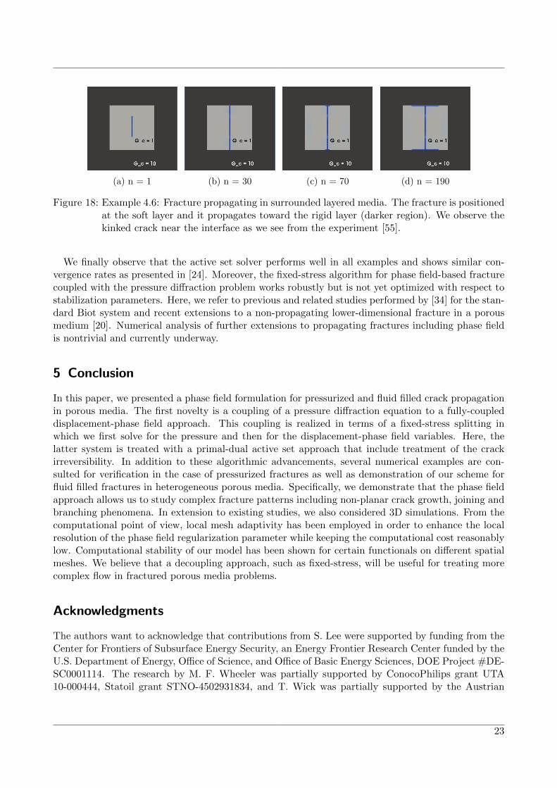
(a) n = 1 (b) n = 30 (c) n = 70 (d) n = 190

Figure 18: Example 4.6: Fracture propagating in surrounded layered media. The fracture is positionedat the soft layer and it propagates toward the rigid layer (darker region). We observe thekinked crack near the interface as we see from the experiment [55].

We finally observe that the active set solver performs well in all examples and shows similar con-vergence rates as presented in [24]. Moreover, the fixed-stress algorithm for phase field-based fracturecoupled with the pressure diffraction problem works robustly but is not yet optimized with respect tostabilization parameters. Here, we refer to previous and related studies performed by [34] for the stan-dard Biot system and recent extensions to a non-propagating lower-dimensional fracture in a porousmedium [20]. Numerical analysis of further extensions to propagating fractures including phase fieldis nontrivial and currently underway.

5 Conclusion

In this paper, we presented a phase field formulation for pressurized and fluid filled crack propagationin porous media. The first novelty is a coupling of a pressure diffraction equation to a fully-coupleddisplacement-phase field approach. This coupling is realized in terms of a fixed-stress splitting inwhich we first solve for the pressure and then for the displacement-phase field variables. Here, thelatter system is treated with a primal-dual active set approach that include treatment of the crackirreversibility. In addition to these algorithmic advancements, several numerical examples are con-sulted for verification in the case of pressurized fractures as well as demonstration of our scheme forfluid filled fractures in heterogeneous porous media. Specifically, we demonstrate that the phase fieldapproach allows us to study complex fracture patterns including non-planar crack growth, joining andbranching phenomena. In extension to existing studies, we also considered 3D simulations. From thecomputational point of view, local mesh adaptivity has been employed in order to enhance the localresolution of the phase field regularization parameter while keeping the computational cost reasonablylow. Computational stability of our model has been shown for certain functionals on different spatialmeshes. We believe that a decoupling approach, such as fixed-stress, will be useful for treating morecomplex flow in fractured porous media problems.

Acknowledgments

The authors want to acknowledge that contributions from S. Lee were supported by funding from theCenter for Frontiers of Subsurface Energy Security, an Energy Frontier Research Center funded by theU.S. Department of Energy, Office of Science, and Office of Basic Energy Sciences, DOE Project #DE-SC0001114. The research by M. F. Wheeler was partially supported by ConocoPhilips grant UTA10-000444, Statoil grant STNO-4502931834, and T. Wick was partially supported by the Austrian

23

Academy of Sciences, The Institute for Computational Engineering and Sciences JT Oden fellowship,and the Center for Subsurface Modeling at UT Austin.

References

[1] G. Allaire, F. Jouve, and N. V. Goethem. Damage and fracture evolution in brittle materialsby shape optimization methods. Journal of Computational Physics, 230(12):5010 – 5044, 2011.ISSN 0021-9991. doi: http://dx.doi.org/10.1016/j.jcp.2011.03.024.

[2] M. Ambati, T. Gerasimov, and L. De Lorenzis. A review on phase-field models of brittle fractureand a new fast hybrid formulation. Computational Mechanics, 55(2):383–405, 2015.

[3] L. Ambrosio and V. Tortorelli. Approximation of functionals depending on jumps by ellipticfunctionals via γ-convergence. Comm. Pure Appl. Math., 43:999–1036, 1990.

[4] L. Ambrosio and V. Tortorelli. On the approximation of free discontinuity problems. Boll. Un.Mat. Ital. B, 6:105–123, 1992.

[5] H. Amor, J.-J. Marigo, and C. Maurini. Regularized formulation of the variational brittle fracturewith unilateral contact: Numerical experiments. Journal of Mechanics Physics of Solids, 57:1209–1229, Aug. 2009. doi: 10.1016/j.jmps.2009.04.011.

[6] M. Artina, M. Fornasier, S. Micheletti, and S. Perotto. Anisotropic mesh adaptation for crackdetection in brittle materials. TUM Report, 2014.

[7] W. Bangerth, T. Heister, G. Kanschat, and M. others. Differential Equations Analysis Library,2012.

[8] S. Berrone, S. Pieraccini, and S. Scial. An optimization approach for large scale simulations ofdiscrete fracture network flows. Journal of Computational Physics, 256(0):838 – 853, 2014. ISSN0021-9991. doi: http://dx.doi.org/10.1016/j.jcp.2013.09.028.

[9] M. J. Borden, C. V. Verhoosel, M. A. Scott, T. J. R. Hughes, and C. M. Landis. A phase-fielddescription of dynamic brittle fracture. Comput. Meth. Appl. Mech. Engrg., 217:77–95, 2012.

[10] B. Bourdin, G. Francfort, and J.-J. Marigo. Numerical experiments in revisited brittle fracture.J. Mech. Phys. Solids, 48(4):797–826, 2000.

[11] B. Bourdin, G. Francfort, and J.-J. Marigo. The variational approach to fracture. J. Elasticity,91(1–3):1–148, 2008.

[12] B. Bourdin, C. Chukwudozie, and K. Yoshioka. A variational approach to the numerical simula-tion of hydraulic fracturing. SPE Journal, Conference Paper 159154-MS, 2012.

[13] A. Bunger and A. Peirce. Numerical Simulation of Simultaneous Growth of Multiple In-teracting Hydraulic Fractures from Horizontal Wells, chapter 21, pages 201–210. doi:10.1061/9780784413654.021.

[14] S. Burke, C. Ortner, and E. Suli. An adaptive finite element approximation of a generalizedAmbrosio-Tortorelli functional. M3AS, 23(9):1663–1697, 2013.

[15] S. Castonguay, M. Mear, R. Dean, and J. Schmidt. Predictions of the growth of multiple inter-acting hydraulic fractures in three dimensions. SPE-166259-MS, pages 1–12, 2013.

24

[16] Z. Chen and Y. Zhang. Well flow models for various numerical methods. International Journalof Numerical Analysis and Modeling, 6(3):375–388, 2009.

[17] Z. Chen, A. Bunger, X. Zhang, and R. Jeffrey. Cohesive zone finite element based modeling ofhydraulic fractures. Acta Mechanica Solida Sinica, 22:443–452, 2009.

[18] G. Francfort and J.-J. Marigo. Revisiting brittle fracture as an energy minimization problem. J.Mech. Phys. Solids, 46(8):1319–1342, 1998.

[19] B. Ganis, M. Mear, A. Sakhaee-Pour, M. Wheeler, and T. Wick. Modeling fluid injection infractures with a reservoir simulator coupled to a boundary element method. ComputationalGeosciences, 18(5):613–624, 2014. ISSN 1420-0597. doi: 10.1007/s10596-013-9396-5.

[20] V. Girault, K. Kumar, and M. Wheeler. Convergence of iterative coupling of geomechanics withflow in a fractured poroelastic medium. ICES report 15-05, Feb 2015.

[21] E. Gordeliy and A. Peirce. Coupling schemes for modeling hydraulic fracture propagation usingthe xfem. Comp. Meth. Appl. Mech. Engrg., 253:305–322, 2013.

[22] E. Gordeliy and A. Peirce. Implicit level set schemes for modeling hydraulic fractures using thexfem. Comp. Meth. Appl. Mech. Engrg., 266:125–143, 2013.

[23] P. Gupta and C. A. Duarte. Simulation of non-planar three-dimensional hydraulic fracture prop-agation. International Journal for Numerical and Analytical Methods in Geomechanics, 38(13):1397–1430, 2014. ISSN 1096-9853. doi: 10.1002/nag.2305.

[24] T. Heister, M. F. Wheeler, and T. Wick. A primal-dual active set method and predictor-correctormesh adaptivity for computing fracture propagation using a phase-field approach. Comput. Meth-ods Appl. Mech. Engrg., 290:466–495, 2015.

[25] M. Heroux, R. Bartlett, V. H. R. Hoekstra, J. Hu, T. Kolda, R. Lehoucq, K. Long, R. Pawlowski,E. Phipps, A. Salinger, H. Thornquist, R. Tuminaro, J. Willenbring, and A. Williams. AnOverview of Trilinos. Technical Report SAND2003-2927, Sandia National Laboratories, 2003.

[26] M. Hintermuller, K. Ito, and K. Kunisch. The primal-dual active set strategy as a semismoothnewton method. SIAM Journal on Optimization, 13(3):865–888, 2002.

[27] A. Katiyar, J. T. Foster, H. Ouchi, and M. M. Sharma. A peridynamic formulation of pressuredriven convective fluid transport in porous media. Journal of Computational Physics, 261(0):209– 229, 2014. ISSN 0021-9991. doi: http://dx.doi.org/10.1016/j.jcp.2013.12.039.

[28] O. Kresse, X. Weng, H. Gu, and R. Wu. Numerical modeling of hydraulic fracture interaction incomplex naturally fractured formations. Rock Mech. Rock Eng., 46(3):555–558, 2013.

[29] B. Lecampion. An extended finite element method for hydraulic fractures. Communications inNumerical Methods in Engineering, 25(2):121–133, 2009.

[30] B. Meyer and L. Bazan. A discrete fracture network model for hydraulically induced fractures-theory, parametric and case studies. In Proceedings SPE Hydraulic Fracturing Technology Con-ference and Exhibition. The Woodlands, Texas, USA. SPE 140514, 2011.

[31] C. Miehe, M. Hofacker, and F. Welschinger. A phase field model for rate-independent crackpropagation: Robust algorithmic implementation based on operator splits. Comput. Meth. Appl.Mech. Engrg., 199:2765–2778, 2010.

25

[32] C. Miehe, F. Welschinger, and M. Hofacker. Thermodynamically consistent phase-field modelsof fracture: variational principles and multi-field fe implementations. International Journal ofNumerical Methods in Engineering, 83:1273–1311, 2010.

[33] C. Miehe, S. Mauthe, and S. Teichtmeister. Minimization principles for the cou-pled problem of darcybiot-type fluid transport in porous media linked to phase fieldmodeling of fracture. Journal of the Mechanics and Physics of Solids, 82:186 –217, 2015. ISSN 0022-5096. doi: http://dx.doi.org/10.1016/j.jmps.2015.04.006. URLhttp://www.sciencedirect.com/science/article/pii/S0022509615000733.

[34] A. Mikelic and M. F. Wheeler. Convergence of iterative coupling for coupled flow and geome-chanics. Comput Geosci, 17(3):455–462, 2012.

[35] A. Mikelic, B. Wang, and M. Wheeler. Numerical convergence study of iterative coupling forcoupled flow and geomechanics. Computational Geosciences, 18(3-4):325–341, 2014. ISSN 1420-0597. doi: 10.1007/s10596-013-9393-8.

[36] A. Mikelic, M. Wheeler, and T. Wick. Phase-field modeling of a fluid-driven fracture in a poroelas-tic medium. Computational Geosciences, pages 1–25, 2015. ISSN 1420-0597. doi: 10.1007/s10596-015-9532-5. URL http://dx.doi.org/10.1007/s10596-015-9532-5.

[37] A. Mikelic, M. F. Wheeler, and T. Wick. A phase-field method for propagating fluid-filled fracturescoupled to a surrounding porous medium. SIAM Multiscale Model. Simul., 13(1):367–398, 2015.

[38] A. Mikelic, M. F. Wheeler, and T. Wick. A quasi-static phase-field approach to pressurizedfractures. Nonlinearity, 28(5):1371–1399, 2015.

[39] B. Noetinger. A quasi steady state method for solving transient darcy flow in complex 3d fracturednetworks accounting for matrix to fracture flow. Journal of Computational Physics, 283(0):205 –223, 2015. ISSN 0021-9991. doi: http://dx.doi.org/10.1016/j.jcp.2014.11.038.

[40] J. Olson. Multi-fracture propagation modeling: Applications to hydraulic fracturing in shalesand tight gas sands. In Proceedings 42nd U.S. Rock Mechanics Symposium. San Francisco, CA,USA. Paper No. 08-327, 2008.

[41] J. Olson et al. Multi-fracture propagation modeling: Applications to hydraulic fracturing inshales and tight gas sands. In The 42nd US rock mechanics symposium (USRMS). AmericanRock Mechanics Association, 2008.

[42] D. Peaceman. Interpretation of well-block pressures in numerical reservoir simulation. Society ofPetroleum Engineers, 1978. doi: 10.2118/6893-PA,SPE-6893-PA.

[43] D. Peaceman. Interpretation of well-block pressures in numerical reservoir simulation with non-square grid blocks and anisotropic permeability. Society of Petroleum Engineers, 1983. doi:10.2118/10528-PA,SPE-10528-PA.

[44] A. Peirce and E. Detournay. An implicit level set method for modeling hydraulically drivenfractures. Comput. Meth. Appl. Mech. Engrg., 197:2858–2885, 2008.

[45] E. Remij, J. Remmers, J. Huyghe, and D. Smeulders. The enhanced local pressure model forthe accurate analysis of fluid pressure driven fracture in porous materials. Computer Meth-ods in Applied Mechanics and Engineering, 286(0):293 – 312, 2015. ISSN 0045-7825. doi:http://dx.doi.org/10.1016/j.cma.2014.12.025.

26

[46] Q. Ren, Y. Dong, and T. Yu. Numerical modeling of concrete hydraulic with extended finiteelement method. Science in China Series E: Technological Science, 52(3):559–565, 2009.

[47] T. Sandve, I. Berre, and J. Nordbotten. An efficient multi-point flux approximation method fordiscrete fracturematrix simulations. Journal of Computational Physics, 231(9):3784 – 3800, 2012.ISSN 0021-9991. doi: http://dx.doi.org/10.1016/j.jcp.2012.01.023.

[48] A. Schluter, A. Willenbucher, C. Kuhn, and R. Muller. Phase field approximation of dynamicbrittle fracture. Comput. Mech., 54:1141–1161, 2014.

[49] I. N. Sneddon and M. Lowengrub. Crack problems in the classical theory of elasticity. SIAMseries in Applied Mathematics. John Wiley and Sons, Philadelphia, 1969.

[50] A. Taleghani. Analysis of hydraulic fracture propagation in fractured reservoirs: an improvedmodel for the interaction between induced and natural fractures. PhD thesis, The University ofTexas at Austin, 2009.

[51] C. V. Verhoosel and R. de Borst. A phase-field model for cohesive fracture. InternationalJournal for Numerical Methods in Engineering, 96(1):43–62, 2013. ISSN 1097-0207. doi:10.1002/nme.4553. URL http://dx.doi.org/10.1002/nme.4553.

[52] M. Wheeler, T. Wick, and W. Wollner. An augmented-Lagangrian method for the phase-fieldapproach for pressurized fractures. Comp. Meth. Appl. Mech. Engrg., 271:69–85, 2014.

[53] T. Wick, S. Lee, and M. Wheeler. 3D phase-field for pressurized fracture propagation in hetero-geneous media. VI International Conference on Computational Methods for Coupled Problems inScience and Engineering 2015 Proceedings, May 2015.

[54] T. Wick, G. Singh, and M. Wheeler. Fluid-filled fracture propagation using a phase-field approachand coupling to a reservoir simulator. SPE Journal, pages 1–19, 2015. doi: 10.2118/168597-PA.

[55] H. Wu, A. Chudnovsky, and J. D. abd G.K. Wong. A map of fracture behavior in the vicinity ofan interface, 2004.

[56] X. Zhang, R. Jeffrey, and M. Thiercelin. Deflection and propagation of fluid-driven fractures atfrictional bedding interfaces: A numerical investigation. J. Struct. Geol, 29(3):396–410, 2007.

27