Embed Size (px)
Citation preview
ICES REPORT 11-24
July 2011
Wavenumber Explicit Analysis for a DPG Method for theMultidimensional Helmholtz Equation
by
L. Demkowicz, J. Gopalakrishnan, I. Muga, and J. Zitelli
The Institute for Computational Engineering and SciencesThe University of Texas at AustinAustin, Texas 78712
Reference: L. Demkowicz, J. Gopalakrishnan, I. Muga, and J. Zitelli, Wavenumber Explicit Analysis for a DPGMethod for the Multidimensional Helmholtz Equation, ICES REPORT 11-24, The Institute for ComputationalEngineering and Sciences, The University of Texas at Austin, July 2011.
WAVENUMBER EXPLICIT ANALYSIS OF A DPG METHOD FORTHE MULTIDIMENSIONAL HELMHOLTZ EQUATION
L. DEMKOWICZ, J. GOPALAKRISHNAN, I. MUGA, AND J. ZITELLI
Abstract. We study the properties of a novel discontinuous Petrov Galerkin (DPG)method for acoustic wave propagation. The method yields Hermitian positive definitematrices and has good pre-asymptotic stability properties. Numerically, we find that themethod exhibits negligible phase errors (otherwise known as pollution errors) even in thelowest order case. Theoretically, we are able to prove error estimates that explicitly showthe dependencies with respect to the wavenumber ω, the mesh size h, and the polynomialdegree p. But the current state of the theory does not fully explain the remarkably goodnumerical phase errors. Theoretically, comparisons are made with several other recentworks that gave wave number explicit estimates. Numerically, comparisons are made withthe standard finite element method and its recent modification for wave propagationwith clever quadratures. The new DPG method is designed following the previouslyestablished principles of optimal test functions. In addition to the nonstandard testfunctions, in this work, we also use a nonstandard wave number dependent norm onboth the test and trial space to obtain our error estimates.
Key words: time harmonic wave propagation; robustness; phase error; dispersion; highfrequency; Petrov Galerkin
1. Introduction
The purpose of this paper is to introduce a Discontinuous Petrov Galerkin (DPG)method for the Helmholtz equation. We analyze the method and give error estimateswith constants whose dependence on the wavenumber are explicitly shown. We also reportresults from many numerical experiments and numerically compare the performance of theDPG method with other methods. Although our theory predicts the same h convergencerates for the DPG method and the standard FEM, the numerical performance of the DPGmethod is far superior for high wave numbers. A striking numerical observation for whichwe do not have a theoretical explanation, is that the DPG method exhibits negligiblephase errors.
The purpose of performing a wavenumber explicit analysis is to track down pollutionerrors and gain a better understanding of how they originate. These errors are wellrecognized as posing severe challenges in numerical simulation of wave propagation [2].For many model problems, the pollution is manifested as phase errors which typicallyaccumulate in the direction of wave propagation over the computational domain. Thusthe concepts of pollution error, phase error, and discrete wave numbers are all closelyrelated. To explain the pollution error in the context of finite element methods, we
Demkowicz and Gopalakrishnan gratefully acknowledge the collaboration opportunities provided bythe IMA (Minneapolis) during their 2010-11 annual program. This work was supported in part by theAFOSR under FA9550-09-1-0608, the NSF under grant DMS-1014817, the FONDECYT project 1110272,and an ONR Graduate Traineeship.
1
2 L. DEMKOWICZ, J. GOPALAKRISHNAN, I. MUGA, AND J. ZITELLI
follow [18]: Given that the exact solution u lies in a space U normed by ‖ · ‖U , and thediscrete solution uh lies in an approximation subspace Uh ⊂ U , one observes that
‖u− uh‖U‖u‖U
≤ C(ω) infwh∈Uh
‖u− wh‖U‖u‖U
, (1)
where ω is the wavenumber, C(ω) = C1 + C2ωβ(ωh)γ, and h is the element size. The
infimum on the right measures the relative best approximation error, which is typicallycontrolled when ωh is small, i.e., when enough elements per wavelength are used. However,the ω-dependence in C(ω), as measured by β, is a reflection of the pollution errors. Formost standard methods of fixed order, the exponent β is observed to be a positive constant.
In contrast, we are able to show that for the new DPG method, quasi-optimality esti-mate (1) holds with C(ω) independent of ω. To be fully accurate, let us add that we willprove so for an “ideal” DPG method. The “practical” DPG method is a simple modifi-cation of the ideal DPG method (both methods will be introduced in Section 2). Notethat the independence of C(ω) with respect to ω does not imply, in theory, that the phaseerrors vanish. This is because the U -norm may still contain ω-dependent terms. Yet, byperforming a wavenumber explicit analysis, we take the first step towards understandingwhy we do not see phase errors in our numerical experiments. We fully analyze the idealDPG method and provide error bounds explicit in the wavenumber ω, the mesh size h,and the finite element polynomial degree p.
By doing so, we are also able to compare our work with a few recent works whichalso give similar wavenumber explicit estimates. (These comparisons are in § 3.2.3.) Forperspective, let us recall the famous negative result of [2] on the inevitability of pollutionerrors. Specifically, Babuska and Sauter [2] worked in the context of a standard methodusing a nine-point stencil (comparable to the standard FEM with bilinear elements). Onethen wonders what happens on more general meshes and methods. It has long beenknown that high order finite elements (with obviously larger stencils) do reduce pollutionerrors. However, a precise statement of this fact was only recently obtained by Melenkand Sauter [22]. We will compare our result with this work. There have been importantrecent developments in DG methods for the Helmholtz equation [12, 13, 16, 23]. Ultraweakformulations, ever since the works of [4, 17], have shown great potential in numericalsolution of the Helmholtz equation, especially those approximations based on plane waves.Most modern DG methods are derived from ultraweak variational formulations. It is notsurprising therefore that a fertile line of attack has been the use of plane waves withinDG trial spaces. New theoretical tools improving the understanding of such methods havejust been developed in the Plane Wave DG (PWDG) method [16]. We will compare ourresults to theirs. Another method we will compare with is an interior penalty methodwith complex stabilization developed in [12, 13]. They also provide an analysis of errorterms characterizing explicitly the dependencies in wavenumber.
That our method is a Petrov-Galerkin method distinguishes it from all the abovementioned works. The guiding principle in designing Petrov-Galerkin methods is thatone chooses trial spaces for good approximation properties, but one designs test spacesto obtain good stability properties. We have exemplified this principle in our earlierworks [7, 8, 9, 25]. In [25], we considered the one-dimensional Helmholtz equation andobtained (1) with C(ω) independent of ω. Unfortunately however, we were not able togeneralize the techniques there to the multi-dimensional case. In this paper, we will pro-vide a different way of theoretical analysis that proves (1) for higher dimensions with
DPG METHOD FOR WAVES 3
C(ω) independent of ω. The new analytical technique is built on the approach developedin [6].
We should note that there are two problems that usually cripple standard numericalmethods for the Helmholtz equation: (i) the growth of the pollution error with frequencyand (ii) the poor approximation of highly oscillatory wave solutions by polynomials. Onecan argue that better trial spaces are needed to overcome the latter. Recent works suchas [16] raise the hope of better trial spaces. However, this is not the subject of thispaper. We concentrate on overcoming the first difficulty by designing better test spaces.Nonetheless, it is important to note that any new developments in approximation spacescan be built into our approach easily. Indeed, our method computes test spaces that pairwith any given trial approximation space.
Finally, let us remark on a practically attractive feature of our DPG method: It yieldsHermitian and positive definite linear systems although the original Helmholtz operatoris indefinite. This is not a surprise if one views the DPG method as a least squaresmethod. Indeed, the DPG method is a least squares method in a nonstandard innerproduct, as clarified in our earlier papers (see e.g., [8, eq. (2.13)]). There have been otherwell known least squares methods, such as FOSLS, for solving the Helmholtz equation,notably [20]. They show a wavenumber-independent stability result if one stays in asubspace sufficiently away from resonant modes (although it is not clear how one maymanage this numerically). They also claim reduced pollution, but the number of meshpoints they use is far higher than what we use to obtain similar accuracy. More interestingare the results they give on multigrid solvers for the least square systems using the ideasof [3]. We hope to borrow these ideas to design efficient solvers for the DPG method, anissue for future research.
The paper is organized as follows. We first describe the DPG method, in the abstract,as well as for the Helmholtz application, in Section 2. In Section 3, we present our mainresult, namely the wave number independent error estimate of Theorem 3.1. A number ofcomparisons with other recent works are also made in this section. In Section 4, we proveTheorem 3.1. In Section 5 we present the results of numerical experiments illustratingthe theoretical results and comparing the DPG method to other standard methods.
2. The ideal and the practical DPG methods
In this section we present the new DPG method. We begin by summarizing the DPGframework developed in [7, 8, 9, 25] in § 2.1. We then apply it to the Helmholtz setting.The method we are able to fully analyze is the method presented in § 2.2. The practicallyimplemented method is described in § 2.3.
2.1. The abstract setting. Let U (the “trial” space) and V (the “test” space) be vectorspaces over the complex field C, and let b(·, ·) : U × V 7→ C be a continuous sesquilinearform. We assume that U is a reflexive Banach space under the norm ‖ · ‖U and that Vis a Hilbert space under an inner product (·, ·)V with a corresponding norm ‖ · ‖V . Thefollowing assumption requires special mention, and we will verify it for the Helmholtzapplication later.
Assumption 1 (Injectivity). We assume that
w ∈ U : b(w, v) = 0, ∀v ∈ V = 0. (2)
4 L. DEMKOWICZ, J. GOPALAKRISHNAN, I. MUGA, AND J. ZITELLI
Now, suppose we are given a continuous conjugate linear form l(v) on V (we use stan-dard terminology – see e.g., [24]). The variational problem we wish to approximate is:
Find u ∈ U such that
b(u, v) = l(v), ∀v ∈ V.(3)
To describe the DPG method for this abstract variational problem, we define
‖v‖opt,V = supw∈U
|b(w, v)|‖w‖U
(4)
and place one more assumption.
Assumption 2 (Norm equivalence). There are positive constants C1, C2 such that
C1‖v‖V ≤ ‖v‖opt,V ≤ C2‖v‖V , ∀v ∈ V. (5)
Clearly, this assumption implies that ‖v‖opt,V is a norm on V . This is called the optimal
test space norm for reasons explained in [25]. Note that the norms ‖v‖opt,V and ‖v‖V arenot equal in general.
The approximate solution of the DPG method lies in a finite dimensional trial subspaceUh ⊂ U . The test space that pairs with the trial space Uh is a subspace Vh ⊂ V that wenow define: First, define the trial-to-test operator T : U 7→ V by
(Tu, v)V = b(u, v), ∀v ∈ V. (6)
Then the discrete test space is set by
Vh = T (Uh). (7)
2.2. The ideal DPG method. The DPG approximation uh ∈ Uh satisfies
b(uh, vh) = l(vh) ∀vh ∈ Vh, (8)
where Vh is as defined in (7). This is a Petrov-Galerkin type formulation as Uh and Vhare not generally identical. Next, we note two basic properties of this method.
The first property is that the stiffness matrix of the method is Hermitian and positivedefinite. Indeed, if ei is a basis for Uh, then setting tj = Tei, we find that the (i, j)-thentry of the stiffness matrix, namely Bij, is
Bij = b(ei, tj) = (ti, tj)V = (tj, ti)V = b(ej, ti) = Bji.
Thus the matrix is Hermitian. To see that it is also positive definite, let c be a complexvector and w = c1e1 + c2e2 + . . . be a basis expansion of any w ∈ Uh. Then, by (6),
c∗Bc = b(w, Tw) = ||Tw||2V . (9)
Now, by Assumption 1, it is obvious that T is injective. By (9), c∗Bc = 0 if and onlyif Tw = 0, which hold if and only if c is the zero vector. As a consequence, we can usepowerful iterative solvers for positive definite systems (like the conjugate gradient method)to obtain the DPG solution, even though the original Helmholtz operator is indefinite.
The second property is a basic convergence result for the abstract method. It is alsoeasy to prove (see [25, Theorem 2.1]), but we omit the proof and simply state it here.
DPG METHOD FOR WAVES 5
Theorem 2.1: Suppose Assumptions 1 and 2 hold. Then problems (3) and (8) are well-posed, and their respective solutions u and uh satisfy the quasi-optimality estimate:
‖u− uh‖U ≤C2
C1
infwh∈Uh
‖u− wh‖U .
2.3. The practical DPG method. In view of the fact that the test space Vh in (7) isdetermined by T , it is natural to ask if this is computationally feasible. As we shall see,the saving grace of the DPG formulation is that T is a local operator and consequentlyinexpensive to approximate. Yet, despite its locality, one must approximate the infinitedimensional T by a local finite dimensional operator T in a computer implementation.I.e., in place of T , we use T : U 7→ V defined by
(T u, v)V = b(u, v), ∀ v ∈ V , (10)
where V is the finite dimensional subspace of V . We will detail our specific choice of Tand V for the Helmholtz application in Section 5. This perturbation of the ideal DPGmethod can be analyzed using the recently developed techniques in [15] and will not bediscussed in this paper. Nevertheless, it is easy to verify that the stiffness matrix of thispractical method is also Hermitian and positive-semidefinite.
2.4. Application to the Helmholtz equation. We consider a bounded domain Ω ⊂Rn (n ≥ 2) with Lipschitz boundary. Let f ∈ L2(Ω) and g ∈ H−1/2(∂Ω). We consider thetime-harmonic wave propagation problem as a first order system. A physically “right”way to do this is via the physics of acoustical disturbances [5]. Linearizing the isentropicEuler equations around a hydrostatic solution and assuming harmonic time variations, weobtain
ıω~u + ~∇φ = ~0, on Ω (11a)
ıωφ+ ~∇ · ~u = f, on Ω (11b)
~u · ~n− φ = g, on ∂Ω, (11c)
where ~u and φ are velocity and pressure variables, respectively, associated to the acousticperturbations from equilibrium. Observe that taking the divergence of (11a) and substi-tuting ~u , we recover the usual second order form of the Helmholtz equation:
−∆φ− ω2φ = ıωf on Ω
∂φ
∂n+ ıωφ = −ıωg on ∂Ω.
Let Ωh be a disjoint partitioning of Ω into open elements K such that Ω = ∪K∈ΩhK.
We multiply the first two equations (11a) and (11b) by test functions and integrate byparts element-wise to obtain an ultraweak DG variational formulation. The details ofthe derivation are very similar to the case of the Poisson equation [6], so we omit themand simply present the DPG weak formulation, after a foreword on notations. Let (·, ·)Ddenote the (sesquilinear) L2(D) inner product on any domain D. The notation 〈·, `〉1/2,∂Kdenotes the action of a linear functional ` in H−1/2(∂K). For concise notation that reflectsthe element by element calculations, we use
(r, s)Ωh:=
∑K∈Ωh
(r, s)K , 〈w, `〉∂Ωh:=
∑K∈Ωh
〈w, `〉1/2,∂K .
6 L. DEMKOWICZ, J. GOPALAKRISHNAN, I. MUGA, AND J. ZITELLI
Note that in the latter definition, complex conjugations are absent, so to match conjugatelinearity of other terms, we will often use notations like 〈w, ¯〉∂Ωh
and 〈w, `〉∂Ωh, whose
meanings are self-explanatory. With these notations, the equations of the method derivedfrom the integration by parts can be stated as follows:
ıω(~u ,~v )Ωh− (φ, ~∇ · ~v )Ωh
+ 〈φ, ~v · ~n〉∂Ωh= 0 ∀~v ∈ H(div, Ωh), (12a)
ıω(φ, η)Ωh− (~u , ~∇η)Ωh
+ 〈η, un〉∂Ωh= (f, η)Ω, ∀η ∈ H1(Ωh). (12b)
Above and throughout, all derivatives are taken element by element unless otherwisementioned, and the ‘broken’ spaces are defined by
H(div, Ωh) = ~τ : ~τ |K ∈ H(div, K), ∀K ∈ Ωh,H1(Ωh) = v : v|K ∈ H1(K), ∀K ∈ Ωh.
From (12), it is clear that there are four solution components, namely ‘interior’ variables
(~u , φ) ∈ L2(Ω)N ×L2(Ω), and the numerical trace and flux (un, φ) which lies in an affinespace Qg, which we now define. Let
Rgdef= (~z , µ) ∈ H(div, Ω)×H1(Ω) : (~z · ~n− µ)|∂Ω = g,
Qgdef= (zn, µ) : ∃(~z , µ) ∈ Rg such that (zn, µ) = tr∂Ωh
(~z , µ),where (zn, µ) = tr∂Ωh
(~z , µ) signifies that for every mesh element K ∈ Ωh, we have
zn|∂K = ~z · ~n|∂K and µ|∂K = µ|∂K .In the case when g = 0, we simply denote R = R0 and Q = Q0. Note that the boundary
condition (11c) becomes an essential boundary condition imposed in the numerical tracespace Qg. Observe that functions in Qg, when restricted to the boundary of a singleelement ∂K, are in H−1/2(∂K)×H1/2(∂K). As already mentioned, the terms involving the
numerical trace φ and the numerical flux un in (12), are to be interpreted as H−1/2(∂K)-functional actions.
Let (~zg, µg) in Rg and let (zg,n, µg) be its corresponding trace in Qg. We look for thesolution, decomposed into
(~u , φ, un, φ) = (~w, ϕ, wn, ϕ) + (~zg, µg, zg,n, µg).
The component (~zg, µg, zg,n, µg), consisting of the data and its extension, is known. Hencewe only need to compute the unknown (~w, ϕ, wn, ϕ). Note that (wn, ϕ) has homogeneousboundary conditions, i.e., it is in Q. We can compute an approximation to the unknown(~w, ϕ, wn, ϕ) by following the abstract program in § 2.1–§ 2.2, with these choices of spacesand forms:
b(
(~w, ϕ, wn, ϕ), (~v , η))
:= ıω(~w,~v )Ωh− (ϕ, ~∇ · ~v )Ωh
+ 〈ϕ, ~v · ~n〉∂Ωh(13a)
+ ıω(ϕ, η)Ωh− (~w, ~∇η)Ωh
+ 〈η, wn〉∂Ωh,
l( (~v , η) ) :=(f, η)Ω − (ıω~zg +∇µg, ~v )Ω − (ıωµg + ~∇ · ~zg, η)Ω, (13b)
U :=L2(Ω)N × L2(Ω)×Q, (13c)
V :=H(div, Ωh)×H1(Ωh). (13d)
The norm on V is defined by
‖(~v , η)‖2V = ‖~∇η + ıω~v ‖2
Ωh+ ‖ıωη + ~∇ · ~v ‖2
Ωh+ ‖η‖2
Ω + ‖~v ‖2Ω,
DPG METHOD FOR WAVES 7
where the derivatives are calculated element by element as usual, while in contrast, thenorm on R is defined using the global distributional derivatives:
‖(~z , µ)‖2R = ‖~∇µ+ ıω~z ‖2
Ω + ‖ıωµ+ ~∇ · ~z ‖2Ω + ‖~z ‖2
Ω + ‖µ‖2Ω.
This in turn defines the norm on Q by standard quotient topology, namely
‖(zn, µ)‖Q = inf‖(~z , µ)‖R : ∀(~z , µ) ∈ R such that tr∂Ωh
(~z , µ) = (zn, µ). (14)
The U -norm is then inherited from the product topology, i.e.,
‖(~w, ϕ, wn, ϕ)‖2U = ‖~w‖2
Ω + ‖ϕ‖2Ω + ‖(wn, ϕ)‖2
Q. (15)
Functions inQ are single valued on element interfaces by definition. They couple unknowninterior values across the mesh elements.
3. The main result and discussion
Our main result is a wavenumber independent quasi-optimality estimate. In this sectionwe state this result (Theorem 3.1). Its proof follows from two results proved in the nextsection. The remaining larger part of this section is devoted to a discussion on convergencerates and how the method compares with a number of recent works by other authors.
3.1. Wavenumber independent quasi-optimality. Our analysis is based on the fol-lowing assumption.
Assumption 3. If φ satisfies
∆φ+ ω2φ = F on Ω (16a)
∂φ
∂n± ıωφ = G on ∂Ω (16b)
for some F ∈ L2(Ω) and G ∈ H 12 (∂Ω), then there is a C > 0 (depending only on Ω) and
an ω0 > 0 such that for all ω > ω0, we have
‖~∇φ‖2Ω + ω2‖φ‖2
Ω ≤ C(‖F‖2
Ω + ‖G‖2∂Ω
). (17)
This assumption is known to hold on bounded convex domains (see [21, Proposi-tion 8.1.4]). It may hold more generally. In fact, a more general assumption of milderpolynomial growth in the solution norm bound is assumed in [22, Assumption 4.7]. How-ever, to our knowledge, while Assumption 3 has been verified for several cases, it is still asubject of active research to verify the more general forms of this assumption on specificdomains.
Theorem 3.1: Suppose Assumption 3 holds. Let U = (~w, ϕ, wn, ϕ) ∈ U be the solutionof the variational problem associated with the spaces and forms defined in (13) and letUh denote its DPG approximation. Then there exist constants ω0 > 0 and C > 0 suchthat the associated DPG solution Uh ∈ Uh satisfies the quasi-optimality estimate
‖U− Uh‖U ≤ C infWh∈Uh
‖U−Wh‖U , ∀ω > ω0.
Here, the constant C is independent of the wavenumber ω, the mesh Ωh, and the approx-imating subspace Uh. The norm ‖ · ‖U is as in (15).
Proof. This follows from Theorem 2.1, whose assumptions –namely Assumptions 1 and 2–are verified in the next section (see Theorem 4.5 and Lemma 4.1).
8 L. DEMKOWICZ, J. GOPALAKRISHNAN, I. MUGA, AND J. ZITELLI
Note that so far, we have assumed nothing about the mesh Ωh or the subspace Uh ⊆ Uin the above theorem. In fact, the theorem applies to arbitrary element shapes and anyapproximating subspace Uh built on any given Ωh. However, it will be useful to considera specific example of Uh obtained using a tetrahedral mesh to facilitate comparison withother works. We do this next.
3.2. Tetrahedral convergence rates. Let us now consider how to use Theorem 3.1 toobtain convergence rates when Ωh is a geometrically conforming, shape regular, tetrahe-dral finite element mesh. Let Pp(D) denote the set of functions that are restrictions of(multivariate) polynomials of degree at most p on a domain D. Let p ≥ 0 and let
Sh,p = ~w : ~w|K ∈ Pp(K)N, Wh,p = v : v|K ∈ Pp(K),Qh,p =
(zn,h, µh) : ∃(~zh,p, µh,p) ∈ R ∩ (Sh,p ×Wh,p)
such that tr∂Ωh(~zh,p, µh,p) = (zn,h, µh)
.
The example we want to consider is the case when the trial space is set by
Uh = Sh,p ×Wh,p ×Qh,p+1. (18)
Clearly, this is a subspace of the space U defined in (13c). We want to derive h and pconvergence rates from Theorem 3.1. As usual, h denotes the maximum of the diametersof all mesh elements. We begin with the simplest case.
3.2.1. The lowest order method. We set p = 0 in (18) to get the lowest order method, i.e.,the interior variables are approximated by piecewise constant approximations, while thenumerical fluxes and traces are piecewise linear. We only need to study the rate at whichthe best approximation term in Theorem 3.1 converges.
To this end, let Ih denote the nodal interpolant of the linear Lagrange finite element,i.e., for a smooth function ψ, the interpolant Ihψ on any K ∈ Ωh is the linear functionwhose values at the vertices of K equal the values of ψ there. By an abuse of notation, weuse the same notation for vector functions, i.e., the vector function obtained by applyingIh to each component of ~v is denoted by Ih~v .
Let (~u , φ) solve the Helmholtz system (11). We tacitly assume that this pair is regularenough to apply the interpolant Ih. Since (~u , φ) satisfies the boundary condition of R, theapproximation pair (Ih~u , Ihφ), by construction, is also in R (as can be seen by comparingthe values of Ih~u · ~n and φ at the Lagrange nodes on each face of K). Furthermore,tr∂Ωh
(Ih~u , Ihφ) is in Qh,p+1, so
inf(vn,h,ψh)∈Qh,p+1
‖(un, φ)− (vn,h, ψh)‖Q ≤ ‖(un, φ)− tr∂Ωh(Ih~u , Ihφ)‖Q.
Since tr∂Ωh(~u , φ) = (un, φ), by the definition of the Q-norm in (14), we have
inf(vn,h,ψh)∈Qh,p+1
‖(un, φ)− (vn,h, ψh)‖Q ≤ ‖(~u , φ)− (Ih~u , Ihφ)‖R. (19)
This is how we bound the best approximation terms for the numerical fluxes. The otherterms forming the total best approximation error in Theorem 3.1 are easier. Combining
DPG METHOD FOR WAVES 9
them with (19),
‖(u, φ, φ, un)− (uh, φh, φh, un,h)‖2U ≤ C
(‖(~u , φ)− (Ih~u , Ihφ)‖2
R
+ inf~wh∈Sh,0
‖~u − ~wh‖2Ω + inf
ψh∈Wh,0
‖φ− ψh‖2Ω
).
By the definition of the R-norm, this implies
‖(u, φ, φ, un)− (uh, φh, φh, un,h)‖2U
≤ C(
ω2‖~u − Ih~u ‖2Ω + ω2‖φ− Ihφ‖2
Ω
+ ‖~∇ · (~u − Ih~u )‖2Ω + ‖~∇(φ− Ihφ)‖2
Ω
+ ‖~u −Π0S~u ‖2
Ω + ‖φ−Π0Wφ‖2
Ω
),
(20)
where Π0S and Π0
W denote the L2-orthogonal projections into Sh,0 and Wh,0, resp. In theabove two inequalities and throughout the paper we use C to denote a generic constantindependent of ω. Its value may differ at different occurrences.
Convergence rates can now be concluded from (20). Note that we used flux and tracespaces of one higher order than the interior trial variables. This means that the middletwo terms on the right hand side in (20) converges at the same h-rate as the last twoterms. By using standard estimates for the L2-projection and the nodal interpolant, (20)implies that
C‖(u, φ, φ, un)− (uh, φh, φh, un,h)‖2U ≤ ω2h2|~u |2H1(Ω) + ω2h2|φ|2H1(Ω)
+ h2|~u |2H2(Ω) + h2|φ|2H2(Ω)
+ h2|~u |2H1(Ω) + h2|φ|2H1(Ω).
At this stage it is convenient to introduce a standard ω-dependent norm (see, e.g. [16]),
‖φ‖2s,ω,D =
s∑j=0
ω2(s−j)|φ|2Hj(D). (21)
Note that if φ is a plane wave eıωx` , then all the terms defining the norm scale with ωin the same way, namely as ω2s. Hence, ‖ · ‖s,ω,D is often considered a natural norm touse for wave propagation problems. We use this norm to summarize the conclusion of theabove discussion.
Corollary 3.2: The DPG solutions in the lowest order tetrahedral case satisfy
‖~u − ~u h‖Ω + ‖φ− φh‖Ω ≤ Ch (‖φ‖2,ω,Ω + ‖~u ‖2,ω,Ω) , (22a)
‖(un, φ)− (un,h, φh)‖Q ≤ Ch (‖φ‖2,ω,Ω + ‖~u ‖2,ω,Ω) . (22b)
Remark 3.1. Note that although the solution component ~u is in H(div, Ω), we used thenodal H1(Ω)-interpolant to approximate it. We did so only because this is an easy wayto find an approximating pair (Ih~u , Ihφ) that satisfies the Robin boundary conditionof R. If one can find a more natural interpolant in R, one may be able to improvethe regularity requirements of the above estimate (e.g., replace ‖u‖2,ω,Ω by the more
appropriate norm ‖~∇ · u‖1,ω,Ω).
10 L. DEMKOWICZ, J. GOPALAKRISHNAN, I. MUGA, AND J. ZITELLI
Remark 3.2. A typical solution of the Helmholtz equation is the plane wave φ = e−ıω~d·~x
and ~u = φ ~d for some unit vector ~d giving the direction of propagation. Then, (22) impliesthat
‖~u − ~u h‖Ω + ‖φ− φh‖Ω ≤ Chω2. (23)
This estimate shows that even if ωh is held constant, the errors increase with ω for fixeddata norms.
Once we fix ωh to be a constant, we may expect the relative best approximation errorto remain more or less constant. Yet the discretization error may not. (Indeed, forthe example in Remark 3.2, as we increase ω, even if we adjust h so that ωh remainsconstant, the discretization errors may grow with ω.) To our knowledge there is nofinite element method to date that can provably avoid this problem in multiple spacedimensions. A manifestation of this error increase with ω, for the standard methods,is via the accumulation of phase errors in the direction of wave propagation. This wasexpounded in [2] in the context of the standard method for the Helmholtz equation, butit also well recognized for Maxwell (see e.g. [14, Fig. 6]) and other wave phenomena.
Surprisingly however, for the DPG method, phase errors were observed to be negligiblein all our numerical experiments. (See Section 5 for an extended discussion.) We arecurrently unable to explain this superior performance theoretically. It is possible that theerror bounds of Corollary 3.2 are too pessimistic.
3.2.2. Higher order convergence. Next, consider the case p ≥ 1. Both h and p convergencerates can be derived from Theorem 3.1 because the constant in the theorem is independentof p. We will now need a conforming p-optimal H1(Ω)-interpolant, e.g., the one givenin [11] and [10, Theorem 8.1], that satisfies
‖ψ −Πhpψ‖Ω + h‖~∇(ψ −Πhpψ)‖Ω ≤ C ln(p)2 hs+1p−s|ψ|Hs+1(Ω),
for all ψ in Hs+1(Ω) with 3/2 < s + 1 ≤ p + 1. Above, p = max(p, 2). For vector func-tions ~v , let Πhp~v denote the vector function obtained by applying Πhp to each componentof ~v . By following the construction of Πhp (see [11]) it is easy to see that the approxi-mating pair (Πhp~u ,Πhpφ) satisfies the boundary condition of R whenever the pair (~u , φ)is in R. Now, we can proceed as in the lowest order case (cf. (20)) to obtain
‖~u − ~uh‖Ω + ‖φ− φh‖Ω + ‖(un, φ)− (un,h, φh)‖Q
≤ C
(ω ln(p)2hsp−s|~u |Hs(Ω) + ω ln(p)2hsp−s|φ|Hs(Ω)
+ ln(p)2hsp−s|~u |Hs+1(Ω) + ln(p)2hsp−s|φ|Hs+1(Ω)
+ hsp−s|~u |Hs(Ω) + hsp−s|φ|Hs(Ω)
).
Overestimating, we can immediately summarize an estimate for the interior variablesusing the norm defined in (21).
Corollary 3.3: The DPG solution in the higher order tetrahedral case satisfies
‖~u − ~uh‖Ω + ‖φ− φh‖Ω ≤ Chsln(p)2
ps(‖φ‖s+1,ω,Ω + ‖~u ‖s+1,ω,Ω) , (24)
for all s = 1, 2, . . . , p.
DPG METHOD FOR WAVES 11
Again, we emphasize that C is independent of ω, h, and p. Obviously a similar estimatecan also be stated for the numerical traces and fluxes.
3.2.3. Comparison with other recent works. Next, we want to compare the above statedconvergence rates with a few other recent works that state error estimates explicitlyshowing the wavenumber dependence. Note that our method simultaneously gives errorestimates for both the pressure φ and velocity ~u . Most other methods give only anapproximation to the primal variable φ. An approximation to the velocity variable ~umust then be derived by numerical differentiation (but this results in a loss of convergenceorder for those methods). Hence, we will only compare error estimates for φ.
(A) The standard p FEM: New estimates for this old method have been derived recentlyin [22]. They show that for domains with analytic boundary, or on convex polygons, if
ωh
pis small and p ≥ C logω, (25)
and additionally if the Helmholtz solution operator’s norm satisfies a polynomial growthassumption (satisfied if Assumption 3 holds) then the solution φh of the standard p-finiteelement method satisfies
ω‖φ− φh‖Ω + ‖~∇(φ− φh)‖Ωh≤ C inf
ψh∈Wh,p∩H1(Ω)
(ω‖φ− ψh‖Ω + ‖~∇(φ− ψh)‖Ωh
)with a C independent of ω. This is perhaps the clearest precise statement available inthe literature demonstrating that pollution effects are removed in high order p FEM. Thisestimate is better than the estimate of our Theorem 3.1. Yet, the numerical performanceof our method (in the case of low p, as reported later) is better than the standard FEM.The main advantage in our theory is that we have no need for condition (25). The DPGmethod has better pre-asymptotic stability properties (e.g., we have no need to assumea sufficiently small h) and yields Hermitian positive definite matrices. The growth ofconditioning with h of both methods are similar.
(B) The plane wave DG method (PWDG): In two space dimensions, the recent pa-per [16, Theorem 3.14] analyzes a Trefftz DG method using plane waves for trial sub-spaces. If plane waves in p′ = 2m + 1 wave directions (sufficiently separated) are usedwith each mesh element, then for sufficiently large p′, they prove that
ω‖φ− φh‖Ω ≤ C(ωh) diam(Ω)hs−1
(ln(p′)
p′
)s−1/2
‖φ‖s+1,ω,Ω (26)
holds for all s < d(m+ 1)/2e, where C(ωh) is an increasing function of ωh. For thesake of comparison when ωh is fixed, we may multiply both sides of (26) by h so thatboth (26) and our estimate (24) gives the same h-convergence rate. If one agrees to viewour polynomial degree p to be more or less comparable to their parameter p′, then ourestimate is comparable to theirs (with the difference that we neither have ω dependencein C, nor do we need to assume large p). However, since we work with polynomial spaces,we avoid the conditioning problems they faced due to the use of plane waves.
We should note however that the numerical results reported in [16] are excellent. Itbegs the question if we could use their same plane wave basis functions to form the trialspace Uh in our DPG setting. Indeed, this can be done. Note that in Theorem 3.1 weplaced no assumptions on Uh, so the theorem applies verbatim in this setting. The onlytheoretical difficulty is in bounding the best approximation error estimate. While the best
12 L. DEMKOWICZ, J. GOPALAKRISHNAN, I. MUGA, AND J. ZITELLI
approximation estimates for the interior variables immediately follow from [16], boundingthe flux best approximation terms seems to require conforming plane wave approximationestimates not available in [16].
(C) Interior penalty DG method with complex stabilization: This method was recentlydeveloped in [12, 13]. In the lowest order case [12, Theorem 5.5 and Eq.(6.6)] they provethat
‖~∇(φ− φh)‖Ωh≤ (1 + ωh)(C1ωh+ C2ω
3h2)
for a specific choice of their stabilization parameters. Here C1 and C2 depend only on theload and are independent of ω and h. We may compare this to our estimate (23). If ωhis held fixed, then the growth with respect to ω in both the estimates are linear. In [13],the higher order case, for a general polynomial degree p, is considered. The best estimatethey have, after an iterative improvement [13, Theorem 5.1], is
‖φ− φh‖Ω ≤ Cωhmin(p+1,s)
ps‖φ‖Hs(Ω), (27)
provided
ω3h2
p≤ C. (28)
The estimate (27) is comparable to (24). A notable difference is the absence of factors ofln(p) in their estimate: These factors arose due to our need to use conforming p-optimalprojectors, a need absent in traditional DG analyses. Also note that we have no need forassumption (28).
4. Analysis
In this section, we verify the assumptions of Theorem 2.1 for the DPG method appliedto the Helmholtz equation. Throughout this section, we tacitly assume that Ω is suchthat Assumption 3 holds for Helmholtz solutions. We show that Assumption 3 impliesAssumptions 1 and 2 for the Helmholtz application.
4.1. Verification of injectivity. To prove the following lemma we only use a weakconsequence of Assumption 3, namely that (17) implies uniqueness of solutions for theHelmholtz problem (16).
Lemma 4.1: Assumption 1 holds for the DPG sequilinear form defined in (13).
Proof. Consider any (~u , φ, un, φ) ∈ U = L2(Ω)N × L2(Ω)×Q satisfying
ıω(~u ,~v )Ωh− (φ, ~∇ · ~v )Ωh
+ 〈φ, ~v · ~n〉∂Ωh= 0,
ıω(φ, η)Ωh− (~u , ~∇η)Ωh
+ 〈η, un〉∂Ωh= 0,
(29)
for all (~v, η) ∈ V = H(div, Ωh) × H1(Ωh). Testing with functions in the subspace of Vconsisting of globally infinitely differentiable functions, compactly supported on Ω, wefind that
ıω~u+∇φ = 0 and ıωφ+ ~∇ · ~u = 0 (30)
in the sense of distributions on the open set Ω. This implies that φ ∈ H1(Ω) and~u ∈ H(div, Ω), which now allows us to integrate by parts in (29). Hence, for every
DPG METHOD FOR WAVES 13
(~v, η) ∈ V , we obtain the equations⟨φ− φ,~v · ~n
⟩∂Ωh
= 0 and 〈η, un − ~u · ~n〉∂Ωh= 0.
Thus, (un, φ) = tr∂Ωh(~u , φ). Furthermore, since (un, φ) ∈ Q, we satisfy the boundary
condition
~u · ~n− φ = 0, over ∂Ω. (31)
Now, we test equation (29) with the globally conforming η = φ ∈ H1(Ω) to get
ıω ‖φ‖2Ω − (~u,∇φ)Ω + ‖φ‖2
∂Ω = 0.
Since ~∇φ = −ıω~u by (30), the real part of this equation implies that ‖φ‖2∂Ω = 0. Hence,
by (31), φ = ~u · ~n = 0 on ∂Ω. Thus, φ satisfies, in a distributional sense, the Helmholtzboundary value problem (16) with zero F and G. Therefore, by Assumption 3, φ = 0 in
Ω. Then, we obviously also have ~u = ~0 in Ω, φ|∂K = φ|∂K = 0 and un|∂K = ~u · ~n|∂K = 0for all K ∈ Ωh.
4.2. Optimal test norm. The optimal norm is easily calculated from its definition (4).Let U = (~w, ϕ, wn, ϕ) ∈ U = L2(Ω)N ×L2(Ω)×Q. Then the bilinear form in (13) can bewritten as
b(U , (~v , η)
)= −(~w, ~∇η + ıω~v )Ωh
− (ϕ, ıωη + ~∇ · ~v )Ωh+ 〈ϕ, ~v · ~n〉∂Ωh
+ 〈η, wn〉∂Ωh.
It is easy to check that in this case, the supremum in the optimal test norm equals
‖(~v , η)‖2opt,V = ‖~∇η + ıω~v ‖2
Ωh+ ‖ıωη + ~∇ · ~v ‖2
Ωh+∣∣[~v , η]
∣∣2∂Ωh
,
where ∣∣[~v , η]∣∣∂Ωh
= sup(wn,ϕ)∈Q
∣∣〈η, wn〉∂Ωh+ 〈ϕ, ~v · ~n〉∂Ωh
∣∣‖(wn, ϕ)‖Q
.
By the definition of the norm on Q, this can be rewritten as∣∣[~v , η]∣∣∂Ωh
= sup(~z ,µ)∈R
∣∣〈η, ~z · ~n〉∂Ωh+ 〈µ,~v · ~n〉∂Ωh
∣∣‖(~z , µ)‖R
.
4.3. Norm Equivalence. Now we turn our attention to verifying Assumption 2. Themain result of this subsection is Theorem 4.5, which verifies the assumption. We be-gin with the following lemma. Recall that the generic constant C is independent of ωthroughout.
Lemma 4.2: Given any η in L2(Ω), there is an ~r ∈ H(div, Ω) and a φ ∈ H1(Ω) suchthat
ıω~r + ~∇φ = 0, on Ω (32a)
ıωφ+ ~∇ · ~r = η, on Ω (32b)
~r · ~n = ±φ on ∂Ω, (32c)
and
‖(~r , φ)‖R ≤ C‖η‖Ω. (33)
14 L. DEMKOWICZ, J. GOPALAKRISHNAN, I. MUGA, AND J. ZITELLI
Proof. Define the sesquilinear form
a±(ϕ, ψ)def= (~∇ϕ, ~∇ψ)Ω − ω2(ϕ, ψ)Ω ± ıω〈ϕ, ψ〉∂Ω.
Let φ ∈ H1(Ω) be the (unique) solution of
a±(φ, ψ) = (ıωη, ψ)Ω, ∀ψ ∈ H1(Ω).
Then, set ~r by ıω~r = −~∇φ. It is easy to see that ~r ∈ H(div, Ω) and (32) is satisfied. To
prove (33), we note that by Assumption 3, we have ‖~∇φ‖2Ω + ω2‖φ‖2
Ω ≤ C‖ıωη‖2Ω. Since
‖ıω~r + ~∇φ‖Ωh= 0, ‖ıωφ+ ~∇ ·~r ‖Ωh
= ‖η‖Ω and ω‖~r ‖Ω = ‖~∇φ‖Ω, we immediately have
ω2‖(~r , φ)‖2R = ω2(‖ıω~r + ~∇φ‖2
Ωh+ ‖ıωφ+ ~∇ · ~r ‖2
Ωh+ ‖~r ‖2
Ω + ‖φ‖2Ω) ≤ Cω2‖η‖2
Ω,
which is (33).
The next lemma is the analogue of Lemma 4.2 for the vector test variable ~v ∈ L2(Ω)N .
Lemma 4.3: There exists an ω1 > 0 such that given any ~v in L2(Ω)N , there is an~r ∈ H(div, Ω) and a φ ∈ H1(Ω) satisfying
ıω~r + ~∇φ = ~v , on Ω (34a)
ıωφ+ ~∇ · ~r = 0, on Ω (34b)
~r · ~n = ±φ on ∂Ω, (34c)
and
‖(~r , φ)‖R ≤ C‖~v ‖Ω (35)
for all ω > ω1.
Proof. First, we set φ ∈ H1(Ω) to be the (unique) solution of
a±(φ, ψ) = (~v , ~∇ψ)Ω, ∀ψ ∈ H1(Ω). (36)
Then, set ~r by ıω~r = −~∇φ+~v . It is easy to see that ~r ∈ H(div, Ω) and (34) is satisfied.It only remains to prove (35). For this, we pick ψ in (36) as ψ = φ+ ζ where ζ ∈ H1(Ω)is the unique solution of the adjoint problem:
a±(ϕ, ζ) = 2ω2(ϕ, φ)Ω ∀ϕ ∈ H1(Ω). (37)
By Assumption 3, we clearly have:
‖~∇ζ‖2Ω + ω2‖ζ‖2
Ω ≤ Cω4‖φ‖2Ω. (38)
Moreover, by (37),
Re(a±(φ, φ+ ζ)
)= Re
(a±(φ, φ)
)+ Re
(a±(φ, ζ)
)= ‖~∇φ‖2
Ω − ω2‖φ‖2Ω + Re(a(φ, ζ))
= ‖~∇φ‖2Ω + ω2‖φ‖2
Ω.
DPG METHOD FOR WAVES 15
Hence,
‖~∇φ‖2Ω + ω2‖φ‖2
Ω = Re(a±(φ, φ+ ζ)
)=(~v , ~∇(φ+ ζ)
)Ω
≤ ‖~v ‖Ω(‖~∇φ‖Ω + ‖~∇ζ‖Ω
)≤ C‖~v ‖Ω
(‖~∇φ‖2
Ω + ω4‖φ‖2Ω
)1/2
.
≤ C ω‖~v ‖Ω(
1
ω2‖~∇φ‖2
Ω + ω2‖φ‖2Ω
)1/2
.
Thus, for large ω, we obtain ‖~∇φ‖2Ω + ω2‖φ‖2
Ω ≤ Cω2‖~v ‖2Ω. Using also the equalities
‖ıω~r + ~∇φ‖Ωh= ‖~v ‖Ω, ‖ıωφ+ ~∇ · ~r ‖Ωh
= 0, and ω‖~r ‖Ω = ‖~v − ~∇φ‖Ω, we obtain
‖(~r , φ)‖2R = ‖ıω~r + ~∇φ‖2
Ωh+ ‖ıωφ+ ~∇ · ~r ‖2
Ωh+ ‖~r ‖2
Ω + ‖φ‖2Ω
≤ ‖~v ‖2Ω +
1
ω2‖~v − ~∇φ‖2
Ω + ‖φ‖2Ω
≤(
1 +2
ω2
)‖~v ‖2
Ω +C
ω2
(‖~∇φ‖2
Ω + ω2‖φ‖2Ω
)≤ C
(1 +
1
ω2
)‖~v ‖2
Ω.
Hence the estimate of the lemma follows taking ω large enough.
Lemma 4.4: There is an ω1 > 0 such that for any (~v , η) ∈ V we have
‖~v ‖Ω + ‖η‖Ω ≤ C ‖(~v , η)‖opt,V ,
for all ω > ω1.
Proof. For a given ~v and η, apply Lemmas 4.2 and 4.3 to obtain (~r , φ) ∈ R satisfying
ıω~r + ~∇φ = ~v , on Ω (39a)
ıωφ+ ~∇ · ~r = η, on Ω (39b)
and
‖(~r , φ)‖R ≤ C (‖~v ‖Ω + ‖η‖Ω) . (40)
Then
‖~v ‖2Ω + ‖η‖2
Ω = (ıω~r + ~∇φ,~v )Ωh+ (ıωφ+ ~∇ · ~r , η)Ωh
(by (39)),
= −(~r , ıω~v + ~∇η)Ω + (~∇φ,~v )Ω + (~r , ~∇η)Ωh
− (φ, ıωη + ~∇ · ~v )Ωh+ (~∇ · ~r , η)Ωh
+ (φ, ~∇ · ~v )Ωh
= −(~r , ıω~v + ~∇η)Ω − (φ, ıωη + ~∇ · ~v )Ωh
+ 〈φ,~v · ~n〉∂Ωh+ 〈η, ~r · ~n〉∂Ωh
(integrating by parts).
16 L. DEMKOWICZ, J. GOPALAKRISHNAN, I. MUGA, AND J. ZITELLI
By Cauchy-Schwarz inequality,
‖~v ‖2Ω + ‖η‖2
Ω ≤(‖~∇η + ıω~v ‖2
Ωh+ ‖ıωη + ~∇ · ~v ‖2
Ωh
)1/2
‖(~r , φ)‖R
+
(∣∣〈φ,~v · ~n〉∂Ωh+ 〈η, ~r · ~n〉∂Ωh
∣∣‖(~r , φ)‖R
)‖(~r , φ)‖R.
so the result follows from (40).
Theorem 4.5: Suppose Assumption 3 holds. Then, there are positive constants ω0, C1, C2
such that for all ω > ω0 and for all (~v , η) ∈ H(div, Ωh)×H1(Ωh),
C1‖(~v , η)‖V ≤ ‖(~v , η)‖opt,V ≤ C2‖(~v , η)‖V .
Proof.Upper bound: We only need to bound the jump term (as the other terms are present in
the V -norm). Since
〈µ,~v · ~n〉∂Ωh+ 〈η, ~z · ~n〉∂Ωh
= (~∇µ,~v )Ωh+ (µ, ~∇ · ~v )Ωh
+ (~z , ~∇η)Ωh+ (~∇ · ~z , η)Ωh
= (~∇µ+ ıω~z ,~v )Ωh+ (µ, ıωη + ~∇ · ~v )Ωh
+ (~z , ~∇η + ıω~v )Ωh+ (ıωµ+ ~∇ · ~z , η)Ωh
≤‖(~v , η)‖V ‖(~z , µ)‖R,
we can divide by ‖(~z , µ)‖R 6= 0 and take the supremum on R to obtain the upper bound.Lower bound: We only need to estimate the two terms in the V -norm that are not in
the optimal norm. But these bounds are immediate by Lemma 4.4 provided ω is largeenough. This finishes the proof.
5. Numerical experiments
In this section we present results of numerical experiments for four distinct modelproblems. In all cases, the results are better than predicted by the preceding theory. Let usbegin by first describing precisely the spaces of approximation used in our computations,and the discrete approximation of the operator T which generates the optimal test space.
We need to specify the trial space (cf. (13c) and (18)). This is constructed using a meshΩh of quadrilaterals. Let Q(l) denote the space of polynomials in one variable of degree atmost l, and let Q(l,m) denote the space of polynomials of degree at most l and m in thetwo variables x1 and x2, resp. We use it to define the sequence of spaces
Xp(K) = Q(p,p), Yp(K) = Q(p,p−1) × Q(p−1,p), Xp−1(K) = Q(p−1,p−1),
for p ≥ 1. These sequence of spaces are to be interpreted as subspaces of H1(K),
H(div, K), and L2(K), resp., where K = (0, 1)2. The spaces Xp(K), Yp(K), Xp−1(K)on a general K ∈ Ωh are the analogous spaces of shape functions on the physical elementdefined through the usual pullback (depending on the subspace interpretation) to the refer-ence element. Similarly, let Q(l)(E) on a (possibly curved) mesh edge E denote the image ofQ(l) from (0, 1) under the standard map. The interior variables are approximated in Sh =~r : ~r |K ∈ Xp(K)N and Wh = v : v|K ∈ Xp(K), resp., while the numerical fluxes and
DPG METHOD FOR WAVES 17
traces lie inQh =
(zn,h, µh) ∈ R : zn,h|E and µh|E are in Q(p+1)(E) for all mesh edges E,
and zn,h − µh = 0 on ∂Ω
, i.e.,
Uh = Sh ×Wh ×Qh.
Note that the numerical traces (in the second component of Qh) are continuous at edgesthat meet at a vertex.
As noted in § 2.3, the practical application of DPG requires us to approximate theoperator T by a discrete version T which maps into a finite dimensional enriched testspace V ⊂ V . In our experiments, V is constructed by considering the local polynomialorder p of the element K and a global parameter ∆p. We compute the practical test spaceusing (10), with V set element by element by
V |K = Yp+∆p(K)×Xp+∆p(K) ⊆ H(div, K)×H1(K).
In all our experiments, we fix ∆p = 2. This choice is dictated by our previous computa-tional experience [6, 8, 9], whereby it was clear that using a higher ∆p did not result inany error improvements, while using a lower ∆p could result in a non-injective T .
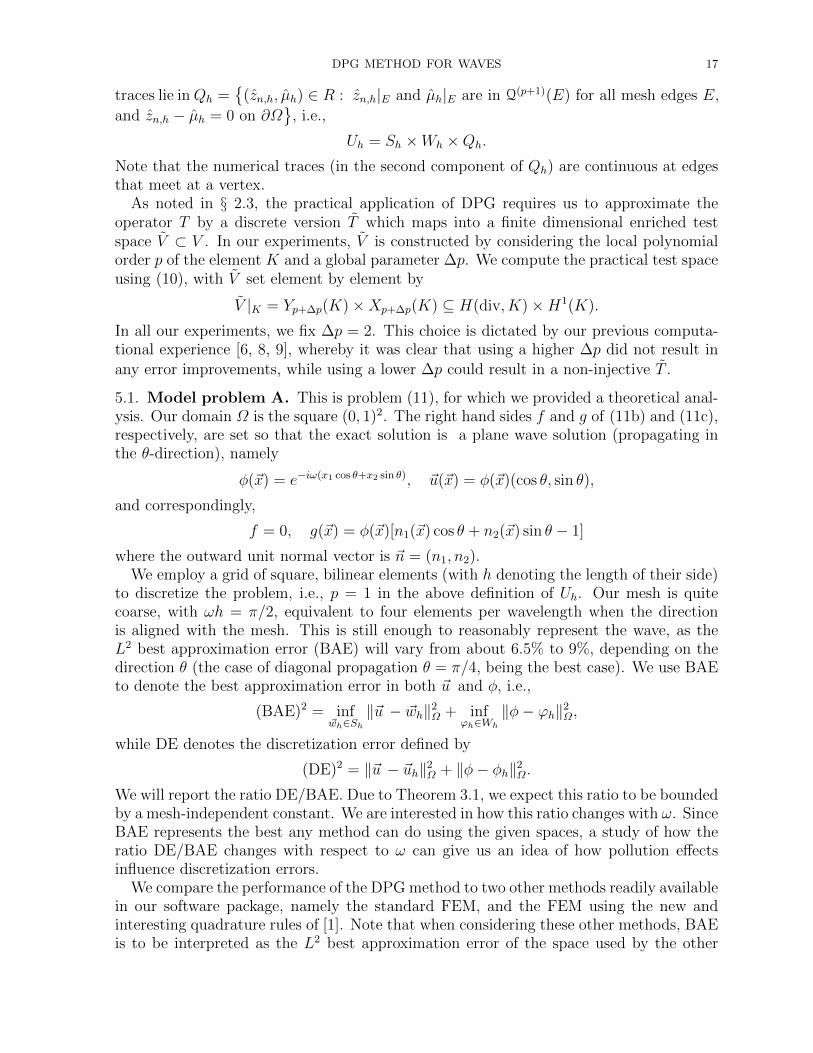
5.1. Model problem A. This is problem (11), for which we provided a theoretical anal-ysis. Our domain Ω is the square (0, 1)2. The right hand sides f and g of (11b) and (11c),respectively, are set so that the exact solution is a plane wave solution (propagating inthe θ-direction), namely
φ(~x) = e−iω(x1 cos θ+x2 sin θ), ~u(~x) = φ(~x)(cos θ, sin θ),
and correspondingly,
f = 0, g(~x) = φ(~x)[n1(~x) cos θ + n2(~x) sin θ − 1]
where the outward unit normal vector is ~n = (n1, n2).We employ a grid of square, bilinear elements (with h denoting the length of their side)
to discretize the problem, i.e., p = 1 in the above definition of Uh. Our mesh is quitecoarse, with ωh = π/2, equivalent to four elements per wavelength when the directionis aligned with the mesh. This is still enough to reasonably represent the wave, as theL2 best approximation error (BAE) will vary from about 6.5% to 9%, depending on thedirection θ (the case of diagonal propagation θ = π/4, being the best case). We use BAEto denote the best approximation error in both ~u and φ, i.e.,
(BAE)2 = inf~wh∈Sh
‖~u − ~wh‖2Ω + inf
ϕh∈Wh
‖φ− ϕh‖2Ω,
while DE denotes the discretization error defined by
(DE)2 = ‖~u − ~uh‖2Ω + ‖φ− φh‖2
Ω.
We will report the ratio DE/BAE. Due to Theorem 3.1, we expect this ratio to be boundedby a mesh-independent constant. We are interested in how this ratio changes with ω. SinceBAE represents the best any method can do using the given spaces, a study of how theratio DE/BAE changes with respect to ω can give us an idea of how pollution effectsinfluence discretization errors.
We compare the performance of the DPG method to two other methods readily availablein our software package, namely the standard FEM, and the FEM using the new andinteresting quadrature rules of [1]. Note that when considering these other methods, BAEis to be interpreted as the L2 best approximation error of the space used by the other
18 L. DEMKOWICZ, J. GOPALAKRISHNAN, I. MUGA, AND J. ZITELLI
101 102 103
1
5
10
15
Wavenumber t (on log scale)
DE/
BAE
DE/BAE with four bilinear elements per wave (e=0)
Standard FEMAW QuadratureDPG method
(a) The θ = 0 case
101 102 103
1
5
10
15
Wavenumber t (on log scale)
DE/
BAE
DE/BAE with four bilinear elements per wave (e=//4)
Standard FEMAW QuadratureDPG method
(b) The θ = π/4 case
Figure 1. Model A: The ratio of discretization errors to best approxima-tion erros in L2(Ω)-norm for two plane wave directions.
method, i.e., BAE= infϕh∈H1(Ω)∩Wh‖φ−ϕh‖Ω, and similarly, DE denotes the discretization
error of the other method. Note also that we use a very modest number of mesh pointsper wavelength (e.g., in comparison to results from other least square methods in theliterature [20]).
The results are in Figure 1 for two values of θ. We observe that in both cases thequality of standard finite element approximations quickly deteriorates as we increase thewavenumber. The deterioration exists, but is delayed, when the method of [1] is used –see the curve labeled “AW Quadrature”. The DPG solutions however are still very closeto the best approximations.
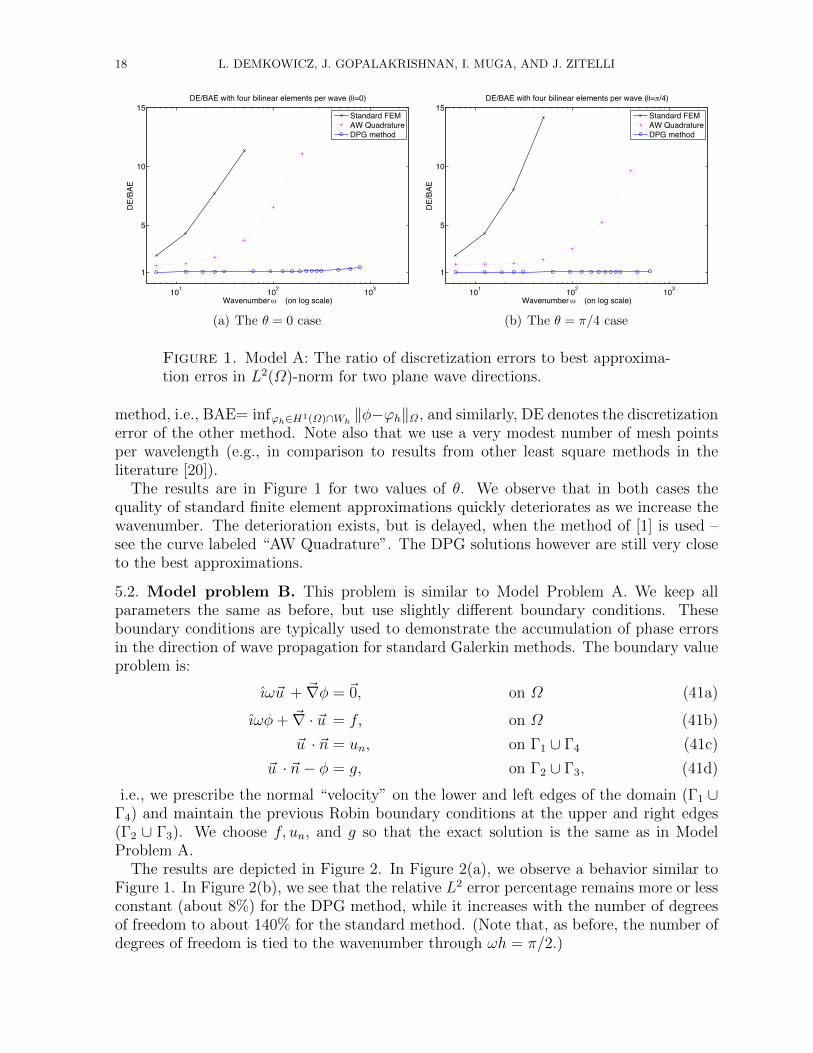
5.2. Model problem B. This problem is similar to Model Problem A. We keep allparameters the same as before, but use slightly different boundary conditions. Theseboundary conditions are typically used to demonstrate the accumulation of phase errorsin the direction of wave propagation for standard Galerkin methods. The boundary valueproblem is:
ıω~u + ~∇φ = ~0, on Ω (41a)
ıωφ+ ~∇ · ~u = f, on Ω (41b)
~u · ~n = un, on Γ1 ∪ Γ4 (41c)
~u · ~n− φ = g, on Γ2 ∪ Γ3, (41d)
i.e., we prescribe the normal “velocity” on the lower and left edges of the domain (Γ1 ∪Γ4) and maintain the previous Robin boundary conditions at the upper and right edges(Γ2 ∪ Γ3). We choose f, un, and g so that the exact solution is the same as in ModelProblem A.
The results are depicted in Figure 2. In Figure 2(a), we observe a behavior similar toFigure 1. In Figure 2(b), we see that the relative L2 error percentage remains more or lessconstant (about 8%) for the DPG method, while it increases with the number of degreesof freedom to about 140% for the standard method. (Note that, as before, the number ofdegrees of freedom is tied to the wavenumber through ωh = π/2.)
DPG METHOD FOR WAVES 19
101 102 103
1
5
10
15
Wavenumber t (on log scale)
DE/
BAE
DE/BAE with four bilinear elements per wave (e=//4)
Standard FEMAW QuadratureDPG method
(a) The DE/BAE ratio for the three methods
101 102 1030
50%
100%
150%
Wavenumber t (on log scale)
Rel
ativ
e L2 e
rror (
in p
erce
ntag
e %
)
Error comparison with four bilinear elements per wave
Standard FEMAW QuadratureDPG method
(b) Relative L2 error (in %) for the three methods
(c) Left: Plot of the error for the CG method showing accumulation of phase errors (atthe northeast corner) in the direction of wave propagation. Right: Plot of the error for theDPG method showing no accumulation of phase errors in the propagation direction.
Figure 2. Results for Model B (all results are for θ = π/4)
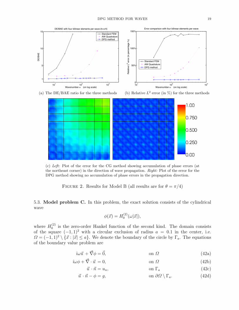
5.3. Model problem C. In this problem, the exact solution consists of the cylindricalwave
φ(~x) = H(2)0 (ω|~x|),
where H(2)0 is the zero-order Hankel function of the second kind. The domain consists
of the square (−1, 1)2 with a circular exclusion of radius a = 0.1 in the center, i.e.Ω = (−1, 1)2 \ ~x : |~x| ≤ a. We denote the boundary of the circle by Γa. The equationsof the boundary value problem are
ıω~u + ~∇φ = ~0, on Ω (42a)
ıωφ+ ~∇ · ~u = 0, on Ω (42b)
~u · ~n = un, on Γa (42c)
~u · ~n− φ = g, on ∂Ω \ Γa. (42d)
20 L. DEMKOWICZ, J. GOPALAKRISHNAN, I. MUGA, AND J. ZITELLI
(a) Mesh when ω = 16π. Note the use ofcurved elements.
101 102 103
1
5
10
Wavenumber t (on log scale)
DE/
BAE
DE/BAE when t h = //2
Standard FEMAW QuadratureDPG method
(b) Ratio of the discretization error to the best ap-proximation error (in L2-norm) for three methods.
10 25 50 100 200 4000
40%
80%
120%
Wavenumber t (on log scale)
Rel
ativ
e L2 e
rror (
in p
erce
ntag
e %
)
Low order DPG vs. higher order methods
p=2: Standard FEMp=2: AW Quadraturep=1: Standard FEMp=1: AW Quadraturep=1: DPG method
(c) The DPG method, at its lowest order (p = 1),compares favorably to other higher order (p = 2)methods.
101 102 1030.8
1
1.2
1.4
1.6
1.8
2
Wavenumber (on log scale)
DE/
BAE
DE/BAE for DPG method when h = /2 and p=1
Model AModel BModel C
(d) A comparison of the performance of DPGmethod for this model and the previous two modelproblems (with zoomed ordinate scale).
Figure 3. Results for Model C.
We discretize using a grid of square elements, with the exception of a block of elementswhich are deformed by geometry mappings generated through transfinite interpolation –see Figure 3(a).
The results are similar to the previous two model problems. The DPG error closelyfollows the L2 best approximation error, as evidenced by the ratio plotted in Figure 3(b),which remains close to the optimal value of 1. These results are for p = 1.
We also compared these results with the p = 2 case of the standard FEM. It is wellknown that increasing the order improves pollution errors for the standard method. Thisis indeed the case, as seen in Figure 3(c), for both the standard FEM and its modificationof [1]. However, even with this improved performance, neither of these methods comparedfavorably to the lowest order DPG method. While the DPG error remained under 9%(in the L2 norm) for the range of wave numbers considered, the L2 errors of the othermethods eventually increased beyond a 100%.
DPG METHOD FOR WAVES 21
Finally, in Figure 3(d), to get an idea of the relative difficulty of the model problemswe considered so far, we compared the performance of the DPG method for Models A,B, and C. The DE/BAE ratio remains close to the optimal value of one for all the threecases. Model A, run with the propagation direction θ = 0 in this plot, seems to show thelargest increase in DE/BAE as the wavenumber increases. (We have run this model tothe limit of our computational resources.) Although this increase is a small fraction ofthe increase the other methods suffer from, the fact that there is a slight increase seemsto indicate that the DPG method may also suffer from pollution errors for large enoughwave numbers. The current data however is insufficient to make a definitive conclusion.
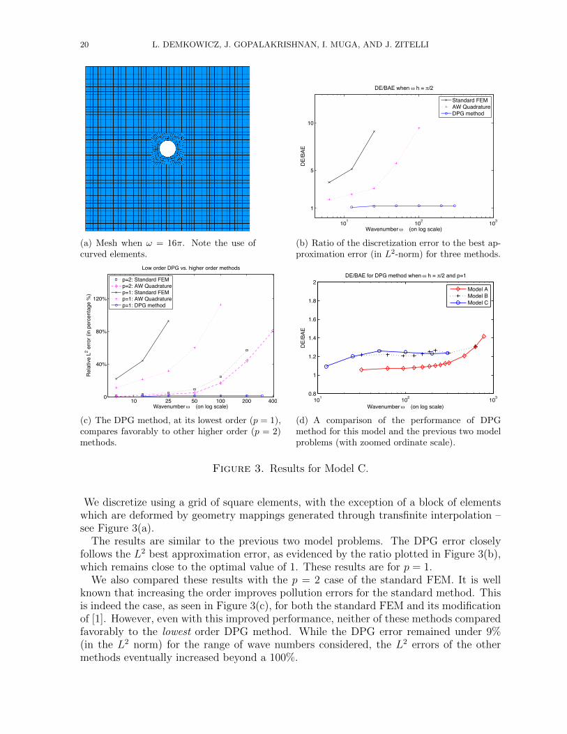
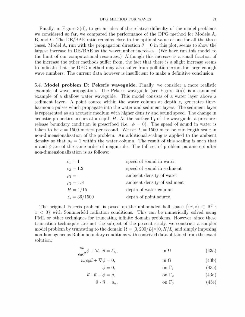
5.4. Model problem D: Pekeris waveguide. Finally, we consider a more realisticexample of wave propagation. The Pekeris waveguide (see Figure 4(a)) is a canonicalexample of a shallow water waveguide. This model consists of a water layer above asediment layer. A point source within the water column at depth zs generates time-harmonic pulses which propagate into the water and sediment layers. The sediment layeris represented as an acoustic medium with higher density and sound speed. The change inacoustic properties occurs at a depth H. At the surface Γ1 of the waveguide, a pressure-release boundary condition is prescribed (i.e. φ = 0). The speed of sound in water istaken to be c = 1500 meters per second. We set L = 1500 m to be our length scale innon-dimensionalization of the problem. An additional scaling is applied to the ambientdensity so that ρ0 = 1 within the water column. The result of this scaling is such that~u and φ are of the same order of magnitude. The full set of problem parameters afternon-dimensionalization is as follows:
c1 = 1 speed of sound in water
c2 = 1.2 speed of sound in sediment
ρ1 = 1 ambient density of water
ρ2 = 1.8 ambient density of sediment
H = 1/15 depth of water column
zs = 36/1500 depth of point source.
The original Pekeris problem is posed on the unbounded half space (x, z) ⊂ R2 :z < 0 with Sommerfeld radiation conditions. This can be numerically solved usingPML or other techniques for truncating infinite domain problems. However, since thesetruncation techniques are not the subject of the present study, we construct a simplermodel problem by truncating to the domain Ω = [0, 200/L]×[0, H/L] and simply imposingnon-homogeneous Robin boundary conditions with contrived data obtained from the exactsolution:
iω
ρ0c2φ+∇ · ~u = δzs , in Ω (43a)
iωρ0~u+∇φ = 0, in Ω (43b)
φ = 0, on Γ1 (43c)
~u · ~n− φ = g, on Γ2 (43d)
~u · ~n = un, on Γ3 (43e)
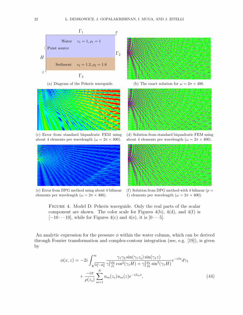
22 L. DEMKOWICZ, J. GOPALAKRISHNAN, I. MUGA, AND J. ZITELLI
H
Γ1
Γ2
Γ3
x
z
Point source
Water c1 = 1, ρ1 = 1
Sediment c2 = 1.2, ρ2 = 1.8
(a) Diagram of the Pekeris waveguide. (b) The exact solution for ω = 2π × 400.
(c) Error from standard biquadratic FEM usingabout 4 elements per wavelength (ω = 2π × 400).
(d) Solution from standard biquadratic FEM usingabout 4 elements per wavelength (ω = 2π × 400).
(e) Error from DPG method using about 4 bilinearelements per wavelength (ω = 2π × 400).
(f) Solution from DPG method with 4 bilinear (p =1) elements per wavelength (ω = 2π × 400).
Figure 4. Model D: Pekeris waveguide. Only the real parts of the scalarcomponent are shown. The color scale for Figures 4(b), 4(d), and 4(f) is[−10 · · · 10], while for Figures 4(c) and 4(e), it is [0 · · · 5].
An analytic expression for the pressure φ within the water column, which can be derivedthrough Fourier transformation and complex-contour integration (see, e.g. [19]), is givenby
φ(x, z) = −2i
∫ ∞√k21−k22
γ1γ2 sin(γ1zs) sin(γ1z)
γ21ρ2ρ1
cos2(γ1H) + γ22ρ1ρ2
sin2(γ1H)e−iβxdγ1
+−iπρ(zs)
N∑m=1
um(zs)um(z)e−iβmx, (44)
DPG METHOD FOR WAVES 23
where k1 = ω/c1,
k2 = ω/c2,
β =√k2
1 − γ21 > 0,
γ2 =√k2
2 − β2 > 0,
and the N modal values βm =√k2
1 − γ21m =
√k2
2 − γ22m > 0 are determined by the N
solutions of the characteristic equation
tan(γ1mH) =iγ1mρ2
γ2mρ1
.
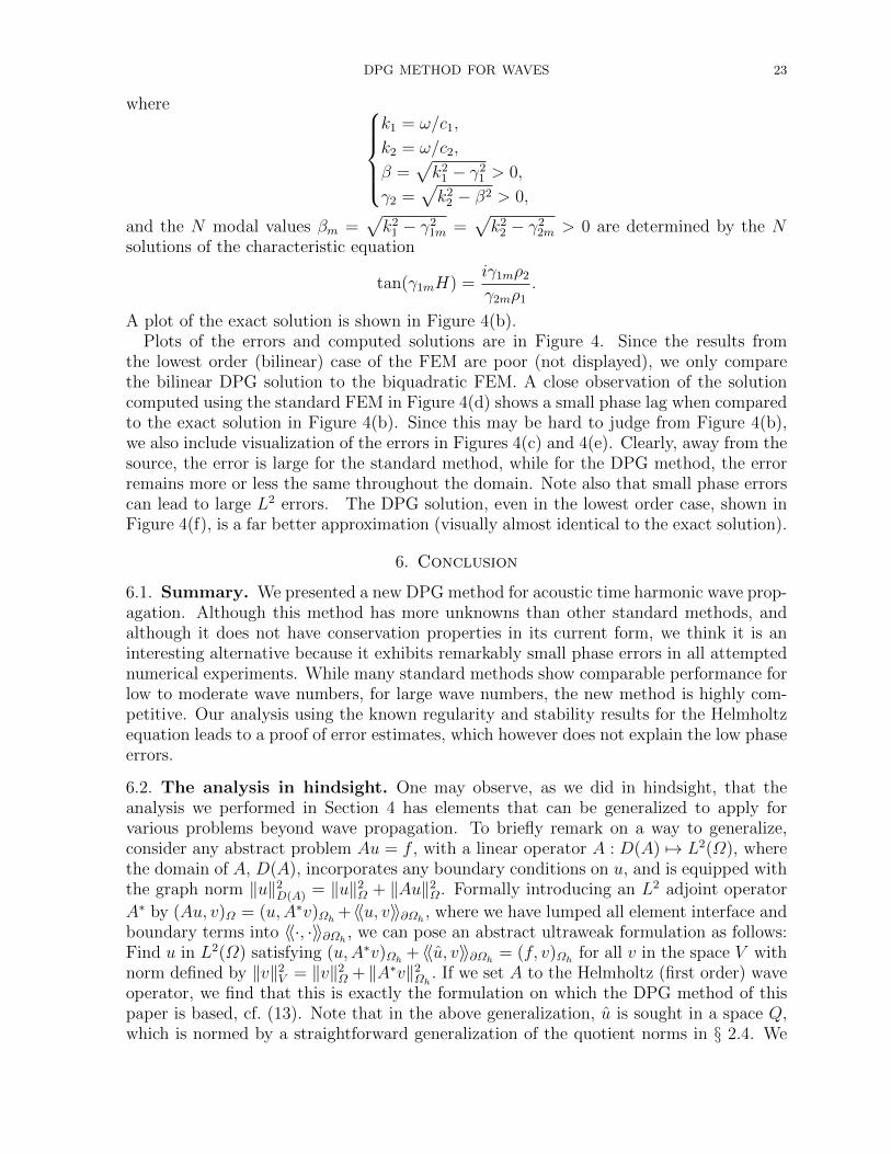
A plot of the exact solution is shown in Figure 4(b).Plots of the errors and computed solutions are in Figure 4. Since the results from
the lowest order (bilinear) case of the FEM are poor (not displayed), we only comparethe bilinear DPG solution to the biquadratic FEM. A close observation of the solutioncomputed using the standard FEM in Figure 4(d) shows a small phase lag when comparedto the exact solution in Figure 4(b). Since this may be hard to judge from Figure 4(b),we also include visualization of the errors in Figures 4(c) and 4(e). Clearly, away from thesource, the error is large for the standard method, while for the DPG method, the errorremains more or less the same throughout the domain. Note also that small phase errorscan lead to large L2 errors. The DPG solution, even in the lowest order case, shown inFigure 4(f), is a far better approximation (visually almost identical to the exact solution).
6. Conclusion
6.1. Summary. We presented a new DPG method for acoustic time harmonic wave prop-agation. Although this method has more unknowns than other standard methods, andalthough it does not have conservation properties in its current form, we think it is aninteresting alternative because it exhibits remarkably small phase errors in all attemptednumerical experiments. While many standard methods show comparable performance forlow to moderate wave numbers, for large wave numbers, the new method is highly com-petitive. Our analysis using the known regularity and stability results for the Helmholtzequation leads to a proof of error estimates, which however does not explain the low phaseerrors.
6.2. The analysis in hindsight. One may observe, as we did in hindsight, that theanalysis we performed in Section 4 has elements that can be generalized to apply forvarious problems beyond wave propagation. To briefly remark on a way to generalize,consider any abstract problem Au = f , with a linear operator A : D(A) 7→ L2(Ω), wherethe domain of A, D(A), incorporates any boundary conditions on u, and is equipped withthe graph norm ‖u‖2
D(A) = ‖u‖2Ω + ‖Au‖2
Ω. Formally introducing an L2 adjoint operator
A∗ by (Au, v)Ω = (u,A∗v)Ωh+ 〈〈u, v〉〉∂Ωh
, where we have lumped all element interface andboundary terms into 〈〈·, ·〉〉∂Ωh
, we can pose an abstract ultraweak formulation as follows:Find u in L2(Ω) satisfying (u,A∗v)Ωh
+ 〈〈u, v〉〉∂Ωh= (f, v)Ωh
for all v in the space V withnorm defined by ‖v‖2
V = ‖v‖2Ω + ‖A∗v‖2
Ωh. If we set A to the Helmholtz (first order) wave
operator, we find that this is exactly the formulation on which the DPG method of thispaper is based, cf. (13). Note that in the above generalization, u is sought in a space Q,which is normed by a straightforward generalization of the quotient norms in § 2.4. We
24 L. DEMKOWICZ, J. GOPALAKRISHNAN, I. MUGA, AND J. ZITELLI
can then view the entire analysis of Section 4 as aimed at proving the equivalence of the‖ · ‖V -norm with the “optimal norm”
‖v‖2opt,V = ‖A∗v‖2
Ωh+∣∣[v]∣∣2∂Ωh
, where∣∣[v]∣∣∂Ωh
= supu∈D(A)
〈〈u, v〉〉∂Ωh
‖u‖D(A)
,
cf. §4.2. The inequality ‖v‖opt,V ≤ C‖v‖V can be proved, even in the general context,exactly as in proof of the upper bound in Theorem 4.5. The gist of the argument toprove the reverse inequality can be abstracted from Section 4, under the assumption that‖u‖Ω ≤ C0‖Au‖Ω. (This assumption follows from Lemmas 4.2 and 4.3 in our particularcase.) Then, given any v ∈ V , considering a u that solves Au = v, we have
‖v‖2Ω = (Au, v)Ω = (u,A∗v)Ωh
+ 〈〈u, v〉〉∂Ωh
≤ ‖u‖Ω‖A∗v‖Ωh+ ‖u‖D(A)
∣∣[v]∣∣∂Ωh
≤(C2
0‖v‖2Ω + (C2
0 + 1)‖v‖2Ω
)1/2(‖A∗v‖2
Ωh+∣∣[v]∣∣2∂Ωh
)1/2
,
which proves that ‖v‖V ≤ C ‖v‖opt,V , thus completing the proof of the norm equivalence.In hindsight, we understand that this is the essence of the analysis not only in this paper,but also in [6].
6.3. Future directions. Our future studies are focused on sharpening our theoreticaltools and formalizing and improving the informally stated abstract generalization above(§ 6.2), all with the aim of proving or disproving that the errors are pollution-free. Anotherdirection of research we are exploring exploits the Hermitian positive definiteness of thelinear system, together with the good phase errors, to design efficient iterative solvers.
Acknowledgements. We are grateful to Markus Melenk for valuable discussions on thetheory in this paper and to David Pardo and Victor M. Calo for constructive criticismson our numerical experiments.
References
[1] M. Ainsworth and H. A. Wajid, Optimally blended spectral-finite element scheme for wavepropagation and nonstandard reduced integration, SIAM Journal on Numerical Analysis, 48 (2010),pp. 346–371.
[2] I. M. Babuska and S. A. Sauter, Is the pollution effect of the FEM avoidable for the Helmholtzequation considering high wave numbers?, SIAM Rev., 42 (2000), pp. 451–484 (electronic). Reprintof SIAM J. Numer. Anal., 34 (1997), no. 6, pp. 2392–2423.
[3] A. Brandt and I. Livshits, Wave-ray multigrid method for standing wave equations, Electron.Trans. Numer. Anal., 6 (1997), pp. 162–181 (electronic). Special issue on multilevel methods (CopperMountain, CO, 1997).
[4] O. Cessenat and B. Despres, Application of an ultra weak variational formulation of ellipticPDEs to the two-dimensional Helmholtz problem, SIAM J. Numer. Anal., 35 (1998), pp. 255–299(electronic).
[5] R. Courant and K. O. Friedrichs, Supersonic Flow and Shock Waves, Interscience Publishers,Inc., New York, N. Y., 1948.
[6] L. Demkowicz and J. Gopalakrishnan, Analysis of the DPG method for the Poisson equation.SIAM J Numer. Anal., 49(5):1788–1809, 2011.
DPG METHOD FOR WAVES 25
[7] L. Demkowicz and J. Gopalakrishnan, A class of discontinuous Petrov-Galerkin methods.Part I: The transport equation, Computer Methods in Applied Mechanics and Engineering, 199(2010), pp. 1558–1572.
[8] , A class of discontinuous Petrov-Galerkin methods. Part II: Optimal test functions, NumericalMethods for Partial Differential Equations, 27 (2011), pp. 70–105.
[9] L. Demkowicz, J. Gopalakrishnan, and A. Niemi, A class of discontinuous Petrov-Galerkinmethods. Part III: Adaptivity, To appear in Applied Numerical Mathematics (2011).
[10] L. Demkowicz, J. Gopalakrishnan, and J. Schoberl Polynomial extension operators. Part III,To appear in Math. Comp., (2011).
[11] L. F. Demkowicz, Polynomial exact sequences and projection-based interpolation with applicationto maxwell equations, in Mixed finite elements, compatibility conditions, and applications, vol. 1939of Lecture Notes in Mathematics, Springer-Verlag, Berlin, 2008, pp. x+235. Lectures given at theC.I.M.E. Summer School held in Cetraro, June 26–July 1, 2006, Edited by Boffi and Lucia Gastaldi.
[12] X. Feng and H. Wu, Discontinuous Galerkin methods for the Helmholtz equation with large wavenumber, SIAM J. Numer. Anal., 47 (2009), pp. 2872–2896.
[13] X. Feng and H. Wu, hp-discontinuous Galerkin methods for the Helmholtz equation with largewave number, To appear in Math. Comp., (2010).
[14] J. Gopalakrishnan and M. Oh, Commuting smoothed projectors in weighted norms with anapplication to axisymmetric Maxwell equations. J. Scientific Computation, DOI: 10.1007/s10915-011-9513-3, 2011.
[15] J. Gopalakrishnan and W. Qiu, An analysis of the practical DPG method. Submitted, 2011.[16] R. Hiptmair, A. Moiola, and I. Perugia, Plane wave discontinuous Galerkin methods for the
2D Helmholtz equation: analysis of the p-version, Tech. Rep. 2009-20, Eidgenossische TechnischeHochschule, 2009.
[17] T. Huttunen, P. Monk, and J. P. Kaipio, Computational aspects of the ultra-weak variationalformulation, J. Comput. Phys., 182 (2002), pp. 27–46.
[18] F. Ihlenburg, Finite element analysis of acoustic scattering, vol. 132 of Applied MathematicalSciences, Springer-Verlag, New York, 1998.
[19] F. B. Jensen, W. A. Kuperman, M. B. Porter, and H. Schmidt, Computational OceanAcoustics. AIP Press, 2000.
[20] B. Lee, T. A. Manteuffel, S. F. McCormick, and J. Ruge, First-order system least-squaresfor the Helmholtz equation, SIAM J. Sci. Comput., 21 (2000), pp. 1927–1949. Iterative methods forsolving systems of algebraic equations (Copper Mountain, CO, 1998).
[21] J. M. Melenk, On Generalized Finite Element Methods, PhD thesis, University of Maryland, 1995.[22] J. M. Melenk and S. Sauter, Convergence analysis for finite element discretizations of the
Helmholtz equation with Dirichlet-to-Neumann boundary conditions. Math. Comp, 79:1871–1914,2010.
[23] R. Tezaur and C. Farhat, Three-dimensional discontinuous Galerkin elements with plane wavesand Lagrange multipliers for the solution of mid-frequency Helmholtz problems, Internat. J. Numer.Methods Engrg., 66 (2006), pp. 796–815.
[24] K. Yosida, Functional analysis, Classics in Mathematics, Springer-Verlag, Berlin, 1995. Reprint ofthe sixth (1980) edition.
[25] J. Zitelli, I. Muga, L. Demkowicz, J. Gopalakrishnan, D. Pardo, and V. Calo, A classof discontinuous Petrov-Galerkin methods. Part IV: Wave propagation, Journal of ComputationalPhysics, 230 (2011), pp. 2406–2432.
26 L. DEMKOWICZ, J. GOPALAKRISHNAN, I. MUGA, AND J. ZITELLI
Institute for Computational Engineering and Sciences, The University of Texas atAustin, Austin, TX 78712.
E-mail address: [email protected]
724 SW Harrison St., Portland State University, Portland, OR 97201.E-mail address: [email protected]
Instituto de Matematicas, Pontificia Universidad Catolica de Valparaıso, Casilla4059, Valparaiıso, Chile.
Institute for Computational Engineering and Sciences, The University of Texas atAustin, Austin, TX 78712.
E-mail address: [email protected]