The Merger of Small and Large Black Holes

P. Mosta1,2, L. Andersson1, J. Metzger1,3, B. Szilagyi1,2, and J. Winicour1,4

1 Max-Planck-Institut fur Gravitationsphysik,Albert-Einstein-Institut, 14476 Golm, Germany2 TAPIR, California Institute of Technology

Pasadena, CA 91125, USA3 Institit fur Mathematik, Universitat Potsdam

14469 Potsdam, Germany4 Department of Physics and Astronomy

University of Pittsburgh, Pittsburgh, PA 15260, USA

We present simulations of binary black holes mergers in which, after the common outer horizon hasformed, the marginally outer trapped surfaces (MOTSs) corresponding to the individual black holescontinue to approach and eventually penetrate each other. This has very interesting consequencesaccording to recent results in the theory of MOTSs. Uniqueness and stability theorems imply thattwo MOTSs which touch with a common outer normal must be identical. This suggests a possibledramatic consequence of the collision between a small and large black hole. If the penetration wereto continue to completion then the two MOTSs would have to coalesce, by some combination of thesmall one growing and the big one shrinking. Here we explore the relationship between theory andnumerical simulations, in which a small black hole has halfway penetrated a large one.

PACS numbers: PACS number(s): 04.20Ex, 04.25Dm, 04.25Nx, 04.70Bw

arX

iv:1

501.

0535

8v1

[gr

-qc]

22

Jan

2015

2

I. INTRODUCTION

An unexpected feature has been observed in the simulation of equal mass binary black holes following their inspiraland merger [1]. After formation of a common apparent horizon, as the two marginally outer trapped surfaces (MOTSs)corresponding to the individual black holes continued to approach, they eventually touched and then penetrated eachother. This penetration was surprising because it had not been considered in theoretical discussions and had not beenobserved in prior simulations of binary black hole mergers. In retrospect, it is tempting to speculate in some heuristicsense that a small black hole should enter a very large black hole with hardly any notice of its presence. In fact,it has been been conjectured on the basis of the equivalence principle that a very small black hole should, in someappropriate sense, fall into the large one along a geodesic. However, such a perturbative picture is unreliable in theinterior of the event horizon surrounding the two black holes, where the MOTSs exist. Here we use an independentevolution code to first confirm that the individual MOTSs do penetrate following a binary black hole merger and weanalyze some of the highly interesting features revealed by the simulations.

The simulations which first demonstrated the penetration of the individual MOTSs were carried out with a codebased upon Fock’s treatment [2] of the harmonic formulation in terms of the densitized metric

√−ggµν , i.e., the PITTAbigel code which had been developed for the purpose of studying outer boundary conditions [3, 4]. By incorporatingadaptive mesh refinement and a horizon tracker available in the CACTUS toolkit [5], the code was further developedto simulate a binary black hole inspiral using excision to deal with the internal singularities. The simulations presentedin the present paper are based upon an independent harmonic code using standard 3 + 1 variables and treating thesingularities via punctures [6] rather than excision [7]. We describe the computational methods in Sec. II.

The seminal work of Hayward [8] and Ashtekar and Krishnan [9] has led to a rich mathematical theory of thedynamical horizons traced out by the evolution of MOTSs, as reviewed in [10]. This theory has provided insight intoboth the classical and quantum properties of black holes. In particular, the subject has strong bearing on numericalrelativity because a MOTS can be identified quasilocally by the vanishing expansion of its outward directed null rays,whereas the identification of an event horizon requires global information which is not available at the early stages ofa simulation. Thus MOTSs play a central role in the preparation of initial data sets for black holes and in trackingtheir subsequent evolution. A numerical study of MOTSs has been carried out [11, 12], which confirmed the mainfeatures expected from the theory regarding the early stages of a binary inspiral. Recently, there has been substantialnew theoretical development centered around the uniqueness and stability of MOTSs [13–16]. This recent theoryapplies to the general case of the marginally outer trapped tube (MOTT) traced out by a MOTS, which need notbe spacelike as in the special case of a dynamical horizon. It has important bearing on how MOTSs approach eachother and penetrate. We review the main mathematical results and their relevance to the binary black hole problemin Sec. III.

The simulations presented in Sec. IV confirm the results observed in [1] and significantly extend the degree ofpenetration of the MOTSs. There are five distinct stages as the MOTSs approach and penetrate.

• The large separation of the individual MOTSs. The properties of this stage are mainly determined by the choiceof binary black hole initial data.

• Formation of a common apparent horizon as the MOTSs approach.

• The moment of external osculation of the two MOTSs as they touch.

• The penetration of the two MOTSs.

• The ultimate fate of the individual MOTSs.

The original simulation showing the penetration of two inspiraling MOTSs [1] and the numerical study of MOTSsin the early stages of a binary black hole [12] were confined to the case of equal mass black holes. Here we consider theunequal mass case, with the goal of shedding light on what happens in the extreme mass ratio regime. Because of thecomputational cost in resolving different length scales, we limit ourselves to the case of a mass ratio msmall/mlarge =1/4. In order to better understand the geometry of the merger, we also restrict ourselves to the simplest case of ahead-on collision. Already in this case, there are quite complicated geometrical effects.

Our simulations are based upon time symmetric initial data for the two black holes. The time symmetry introducessome non-intuitive features of the initial MOTSs, particularly when they are close together, which emphasize theimportance of looking at their invariant geometrical properties rather than their coordinate description. We repeat,for the unequal mass case, the simulation of the head-on collision carried out by Krishnan and Schnetter [12] for equalmass black holes. They simulated this equal mass case with a code based upon a 3 + 1 formulation of Einstein’sequations (the AEI BSSN formulation), which is quite different from the harmonic formulation used here. As a checkon our code, we find qualitative agreement with the results of [12] for the early stages before the individual MOTSs

3

touch. We then continue the simulation of the head-on collision to the later stage where the individual MOTSspenetrate, which could not be treated in [12].

The original simulations of the penetration in [1] were limited by the excision region inside the individual MOTSs.The present code is able to track the penetration to a much further stage, essentially until the small MOTS haspenetrated halfway into the large MOTS. At that stage its interior puncture is close to the surface of the large MOTSand the horizon finder is not able to track it. The simulation of the penetration is validated by the convergencemeasurements given in Sec. IV E.

We demonstrate by numerical simulation that before the individual MOTSs make contact a common outer apparenthorizon forms, in accord with the theory described in Sec. III. When the two MOTSs first touch, the theory also predictsthat their mean surface curvatures must agree at the point of osculation. Consistent with this theory, our simulationsshow that the small MOTS creates a strong distortion of the large MOTS at the contact point which causes the meancurvature of the large MOTS to grow rapidly at the point of contact, i.e. its curvature radius rapidly shrinks. Onthe other hand, at this stage the large MOTS has only a small effect on the small one. We track this growth ofmean curvature of the large MOTS as the penetration proceeds. In a scenario where the black holes are produced bycollapsing matter, without any puncture, one might expect the penetration to continue to the point where the smallMOTS completely penetrates the large one. If this were to occur, then a dramatic consequence of the underlyinguniqueness theorems for MOTSs would ensue. At the time where the back of the small MOTS enters the front of thelarge one, the theorems imply that the two MOTSs must identically coalesce, either through shrinkage of the largeMOTS or growth of the small MOTS. Although our simulations cannot proceed to this stage, they provide someglimpse of how it might proceed.

II. COMPUTATIONAL METHOD

A. The evolution system

We employ an evolution system based upon the 3+1 formulation of Einstein equations in generalized harmoniccoordinates xµ = (t, xi) as described by Friedrich and Rendall [17]. (We make minor alterations in the notation of [17]to conform to standard usage in numerical relativity.) This 3+1 foliation gives rise to the metric decomposition

gµν = −nµnν + hµν (2.1)

where

nµ = −α∂µt, α =1√−gtt

(2.2)

is the unit future directed timelike normal to the foliation. The evolution proceeds along the streamlines of the vectorfield ∂t = αnµ∂µ + βµ∂µ determined by the lapse α and shift βµ = (0, βi).

In this formulation the constraints are

Cµ := Γµ − Fµ (2.3)

where Γµ is related to the Christoffel symbols by Γµ = gρσΓµρσ and Fµ(g, x) are harmonic gauge source functions [18].

When the harmonic constraints are satisfied, i.e. Cµ = 0, the Einstein equations reduce to a system of quasilinearwave equations for the spatial metric hij , shift βi and lapse α which take the form [17]

− gµν∂µ∂νhij = Sij (2.4)

1

α2

(∂t − βj∂j

)2βi − hjk∂j∂kβi = Si (2.5)

1

α2

(∂t − βj∂j

)2α−DjD

jα = S, (2.6)

where Di is the covariant derivative associated with hij and the right-hand-side S-terms do not enter the principal

4

part. In detail, these terms are

Sij =2

α2Kij (∂tα− Lβα) +

2

α2DiαDjα (2.7)

−2D(i

[hj)kh

kνF

ν]

+4

α3D(iαhj)k

(∂tβ

k − β`∂`βk)

+4

α2

(∂(jβ

k)∂thi)k +

2

α2h`(i

(∂j)β

k) (∂kβ

`)

− 2

α2

(∂(jβ

k)Lβhi)k −

2

α2

(∂(jβ

k) (∂`hi)k

)+4KikK

kj − 2KijK − 2γ`kihn`g

kmγnmj − 4γ`kmhknh`(iγ

mj)n +Bij

Si = 4(Ki` −Khi`

)D`α (2.8)

−2α(Km` −Khm`

)γi`m −

(∂`β

i)γ`

+(∂`β

i)D` logα

+2αnνFν[γi −Di logα− hiνF ν

]−2αKhiνF

ν −Di (αnνFν)−

(∂t − βk∂k

) (hiνF

ν)

+Bi

S = −α[KijK

ij − 4KnνFν − 2 (nνF

ν)2 − 2K2

](2.9)

+(∂t − βk∂k

)(nνF

ν) +B,

where γkij are the Christoffel symbols associated with Di, γk = hijγkij , Kij = (1/2α)(∂t − Lβ)hij is the extrinsic

curvature of the Cauchy foliation and the quantities B,Bi, Bij are constraint modification terms defined in (2.20)-(2.22) which are used to stabilize the constraint propagation system. With the addition of constraint modification,(2.4)-(2.6) correspond to equations (2.33), (2.36) and (2.38) of [17], as corrected for typographical errors. See [19] forfurther details.

Constraint preservation for the Cauchy problem follows from the system of homogeneous wave equations satisfiedby the harmonic constraints (2.3). Constraint propagation can be extended to the initial-boundary value problemby implementing the hierarchy of Sommerfeld outer boundary conditions presented in [4, 20]. However, this has notyet been incorporated in the version of the code being used here and we maintain constraint preservation by causallyisolating the region of interest from the outer boundary.

For the purpose of using the method of lines to apply a Runge-Kutta time integrator, we re-write the system(2.4)-(2.6) as first differential order in time and second differential order in space by using the timelike vector field

nν =1

α(δν0 − wβν) (2.10)

to introduce the auxiliary variables

Π := Lnα = nµ∂µα (2.11)

Πi := Lnβi = nµ∂µβ

i − βk∂kni (2.12)

Πij :=1

2Lngij =

1

2[nµ∂µhij + giµ∂j n

µ + gjµ∂inµ] . (2.13)

Here the function w is chosen to be unity everywhere except near the boundary, where it smoothly goes to zero.Insertion of (2.10) into (2.11)-(2.13) gives the evolution equations for the lapse, shift and 3-metric,

∂tα = αΠ + wβi∂iα (2.14)

∂tβi = αΠi +

w

αβiβk∂kα− βiβk∂kw (2.15)

∂thij = 2αΠij − α[nk∂khij + giµ∂j n

µ + gµj∂inµ]. (2.16)

The evolution equations for the auxiliary Π-variables then follow from the first time derivatives of (2.14)-(2.16), afterusing (2.14)-(2.16) and (2.4)-(2.6) to eliminate first and second time-derivatives of the metric variables.

We modify the evolution system by terms vanishing modulo the constraints based upon the results presented in [3].For this purpose we set

Aµν = − a1√−gCα∂α

(√−ggµν)+a2Cα∇αt

ε+ eρσCρCσCµCν − a3√

−gttC(µ∇ν)t (2.17)

5

where ε is a small positive number, ai are positive parameters and

eµν = nµnν + hµν (2.18)

is a Riemannien 4-metric. In terms of

Aµν = gµσgνρAσρ − 1

2gµνgρσA

ρσ (2.19)

the B-terms added to (2.7)-(2.9) for constraint modification are

B =1

α

(−βiβjAij + 2gijβ

jβkgilAkl + 2gijβjgikAtk

)(2.20)

Bi = −2(βjgikAkj + gijAtj

)(2.21)

Bij = −2Aij . (2.22)

B. Numerical implementation

The evolution algorithm uses fourth order centered finite differencing and sixth order Kreiss-Oiliger type dissipationon a cubic Cartesian grid. The outer boundary points are updated using a Sommerfeld algorithm provided by theCactus toolkit [5], while we use summation-by-parts finite difference operators to update the neighboring three pointsalong the normal Cartesian axis.

In addition, following the lead of the BSSN method for treating punctures, we compute the spatial derivatives ofthe 3-metric hij using the conformal rescaling

hij = h−1/3hij (2.23)

to obtain

∂khij = hij∂kh1/3 + h1/3∂khij (2.24)

∂k∂`hij = hij∂k∂`h1/3 +

(∂`h

1/3)(

∂khij

)(2.25)

+(∂kh

1/3)(

∂`hij

)+ h1/3∂k∂`hij ,

where derivatives of hij are computed using finite difference operators. The derivatives of the conformal factor h1/3

are computed using

∂kh1/3 = h1/3∂k

[log(h1/3

)](2.26)

∂k∂`h1/3 = h1/3∂k

[log(h1/3

)]∂`

[log(h1/3

)]+ h1/3∂k∂`

[log(h1/3

)], (2.27)

where the finite difference operators are applied to the quantity[log(h1/3

)].

In addition to the Cactus infratructure we use Carpet mesh refinement [21, 22]. The MOTSs are tracked using thehorizon finder developed by J. Thornburg [23, 24], which decomposes a topologically spherical surface into 6 abuttingcubical patches. This finder is based upon a search algorithm which assumes a star-shaped domain inside the horizon.

As this is the first example of harmonic evolution of black holes using the puncture method, as opposed to excision,we adopt a conservative approach to insure that the puncture never lies exactly on a grid point. This is made possiblein the simulation of a head-on collision by offsetting the puncture a half grid-step from the axis along which thecollision proceeds. In addition, for simulation of a head-on collision, harmonic gauge forcing is not necessary and weset Fµ = 0. Further studies and code development would be necessary to better understand the harmonic applicationof the puncture method so that the code could handle generic binary inspirals. With the present techniques, however,we can evolve the head-on collision for time scales well past the formation of a common apparent horizon and are ableto track the subsequent penetration of the individual MOTSs.

6

III. THEORY OF THE UNIQUENESS AND STABILITY OF MOTSS

Again consider a 3+1 foliation xα = (t, xi) with metric decomposition

gµν = −nµnν + hµν , (3.1)

where nµ is the unit future directed timelike normal to the foliation. In a slice Mτ := t = τ consider a 2-surface Swhich is the boundary of a set Ω. We define its outward unit spacelike normal Ni to point out of Ω. If S is definedas the level set of a function s, then

Ni =1√D∂is (3.2)

with

D = hkl(∂ks)(∂ls). (3.3)

Setting Nµ = hiµNi (so that Nµ∇µt = 0), this leads to the further decomposition

hµν = NµNν + sµν . (3.4)

The outgoing null direction normal to S is

`µ = nµ +Nµ, (3.5)

where the normalization is determined by the Cauchy slicing. The expansion in this outgoing null direction is

θ+ = P +H (3.6)

where

H = sµν∇µNν (3.7)

is the mean curvature of S in the Cauchy slicing,

P = sµν∇µnν (3.8)

is the 2-trace of the extrinsic curvature of the Cauchy slicing and ∇ is the covariant derivative with respect to g.S is a MOTS if θ+ = 0, i.e. P +H = 0. Similarly,

θ− = P −H (3.9)

is the expansion in the ingoing null direction

kµ = nµ −Nµ (3.10)

normal to S. The MOTS S is inner trapped if θ− < 0. Since θ− = θ+ − 2H = −2H for a MOTS, the trappingcondition is equivalent to H > 0.

A. Stable and outermost MOTSs

For a given slice Mτ and a MOTS S ⊂ Mτ one can consider the normal graphs Su of a function u ∈ C∞(S), i.e.the surface parametrized by

Fu : S →Mτ : p 7→ exp(uN i) (3.11)

where exp denotes the exponential map of Mτ . The operator Θ+ : C∞(S)→ C∞(S) that maps a function u to thepull-back of the value of θ+ on Su to S has linearization given by

Lf = −∆f − 2sABSA∂Bf + f( 12RS − SASA +DASA − 1

2χABχAB −Gµν`µkν) (3.12)

7

with ∆ the surface Laplacian of S, Sµ = Nν∇µnν , RS denotes the scalar curvature of S, χµν = ∇µ`ν , Gµν denotesthe Einstein tensor of the space-time and capital letters refer to intrinsic coordinates xA for S. In particular sAB

denotes the inverse of the tangential projection of sµν to S.Although L is not self-adjoint, there exists a real eigenvalue λ(S) ∈ σ(L), which is the unique minimizer for the

real part in the spectrum σ(L) of L. This eigenvalue is simple, and the corresponding eigenfunction φ can be chosenwith a definite sign. If λ(S) ≥ 0 we say that S is stable, if λ(S) > 0 it is called strictly stable. We refer to [14, 15] forfurther details.

For the following, we require the surfaces S in question to be either bounding, S = ∂Ω, or bounding with respectto an interior boundary ∂M, that is S = ∂Ω \ ∂M. In both cases, we write S = ∂+Ω or refer to S being an outerboundary in this situation. In the scenario considered here, the inner boundary exists and is formed by trappedsurfaces enclosing the punctures.

A MOTS S = ∂+Ω is called outermost if for all other MOTSs S ′ = ∂+Ω′ with Ω′ ⊃ Ω it follows that Ω′ = Ω. Inother words, there are no MOTSs on the outside of S.

In [25] it was shown that ifMτ contains bounding outer trapped surfaces, as is the case ifMτ is asymptotically flat,then there exists an outermost MOTS Sout that bounds the trapped region inMτ . This means, it is the enclosure ofthe region that contains outer trapped surfaces. Note that Sout is not necessarily connected. All components of Sout

are stable, and Sout has area bounded uniformly from above by a constant depending only on the geometry of theslice Mτ . Furthermore, it has the property that there exists a positive δ > 0, again depending only on the geometryof the sliceMτ , such that any geodesic starting on Sout in direction of its outward normal N i does not intersect Sout

within distance δ. In particular, two distinct components of Sout have distance at least δ. The constants mentioneddepend in particular on an intrinsic curvature bound and on bounds for the second fundamental form ∇µnν and itsderivatives. For the details of these estimates and all the dependencies of the constants we refer to [25]. Similar resultshave also been derived in [26, 27]. In the situation considered here, Galloway [29] established that Sout is a union oftopological spheres. In [28] it has been furthermore established that the second fundamental form ∇iNj of a stableMOTS S is bounded in the supremum norm, provided the geometry of the slice is bounded.

B. The maximum principle for MOTSs

A useful tool in the analysis of MOTSs is the strong maximum principle. To state it, assume that Sα for α = 1, 2are two connected C2-surfaces with outer normals N i

α. Assume further that there is a point p such that S1 and S2

touch at p. If the outer normals agree, N i1 = N i

2, at p and S2 lies to the outside of S1, that is in the direction of N i1,

and furthermore

supS1

θ+[S1] ≤ infS2θ+[S2] (3.13)

then S1 = S2. This version can be found in [25, Proposition 2.4] or in [16]. It implies in particular that two distinctMOTSs S1 and S2 can not touch in such a way that their normals point in the same direction and one is enclosingthe other.

The strong maximum principle provides an interpretation of strict stability. Assume that S is a strictly stable MOTSwith outward normal N i. Let φ be the principal eigenfunction of L. Deforming S in direction of the vector field φN i

then yields a foliation of a tubular neighborhood U of S with the following properties. First U \ S = U− ∪U+ whereN i points into U+. Moreover, U+ is foliated by surfaces with θ+ > 0 and U− is foliated by surfaces with θ+ < 0. Themaximum principle then implies that there are no surfaces S ′ ⊂ U+ which bound relative to S and have θ+[S ′] ≤ 0.Furthermore, there is no MOTS in U with outward normal aligned with that of S.

C. Evolution of MOTSs to MOTTs

Regarding the evolution of MOTSs there are different approaches. In [14] it was shown that a strictly stableMOTS S can locally be continued to a smooth space-time track of MOTSs, i.e. a marginally outer trapped tube.More precisely, for a given τ such that Mτ contains a strictly stable MOTS Sτ there exists ε > 0 such that for allτ ∈ (τ −ε, τ +ε) there is a stable MOTS Sτ inMτ such that the Sτ form a smooth space-like manifold. To emphasizethe role of the stability operator in this picture, we recall the argument from [14]. Assume that Sτ is a smooth familyof MOTSs passing through Sτ . Then we can parametrize this tube by a map

Fµ : (τ − ε, τ + ε)× Sτ →⋃

τ∈(τ−ε,τ+ε)

Mτ (3.14)

8

such that ∂Fµ

∂τ = V µ, where V µ is perpendicular to Sτ at each point along the tube. Note that V µ has the decompo-sition

V µ = αnµ + γNµ = α(nµ +Nµ) + (γ − α)Nµ = α`µ + fNµ, (3.15)

where as before α denotes the lapse function of the slicing. Calculating the change of θ+ under the deformation byV µ at time τ , we thus obtain

δV µθ+[Sτ ] = δα`µθ+[Sτ ] + δfNµθ+[Sτ ] = −αW + Lf, (3.16)

where the first contribution is calculated via the Raychaudhuri equation with

W = χABχAB +Gµν`µ`ν , (3.17)

and the second part is just the definition of the stability operator (3.12). Since V µ is tangent to a MOTT we haveδV µθ+[Sτ ] = 0 and thus

Lf = αW. (3.18)

The operator L and the function W are given by the geometry of Sτ and the space-time geometry of Mτ , whereasf is a function determined by (3.16). If Sτ is strictly stable then L is invertible. Thus the previous calculation canbe turned around to conclude the existence of the desired MOTT. The causal structure of the tube follows by theobservation that the null energy condition implies W ≥ 0. From stability one then obtains f ≥ 0 via equation (3.18)as in [14, Lemma 3].

A similar argument was used in [13] to construct a MOTT through Sτ in the case it is stable but not strictly stableassuming W ≥ 0 and W 6≡ 0.

A different approach is to take the outermost MOTS Soutτ of all slices Mτ and define the apparent horizon of the

slicing as H =⋃τ Sout

τ . In generic space-times H is smooth up to a discrete set of outward jumps. See [13] for thedetails and the particular notion of genericity used therein. The same reference also provides the causal character ofH, namely that H is achronal. Moreover, if Ωτ denotes the interior of Sout

τ , then J+(Ωτ ) ∩Mσ ⊂ Ωσ for all τ < σ.Here J+(Ωτ ) denotes the causal future of Ωτ . In particular, if there is a MOTS at an initial time τ then it will persistfor all times.

D. Approaching MOTSs

Assume that the space-time and the slicing are completely regular. Then the constant δ, the bound for the area, andthe length of the second fundamental form of Sout remains uniformly controlled. If in this situation two componentsof a MOTS are closer than δ, neither of these two components can be part of Sout. In particular, the evolution ofSout will be discontinuous at some stage of the evolution. By the causality of H, the jump is outward, and a newoutermost MOTS has formed outside the tubes of the two original ones. Generically, after the jump time the jumptarget will split into two branches of MOTTs, a stable branch traveling outward and an unstable branch travelinginward. For a complete discussion of this jump in the outermost MOTS, we refer to [13]. An important fact to pointout is that if two MOTSs are close to each other then there is no reason to expect that they be stable, in contrast tothe stability of Sout.

Note that it is not known whether the area of Sout is monotonic across the jumps. For MOTSs in general, includingSout, it is not even clear whether monotonicity of area should be expected along smooth pieces. However, if theMOTS has positive mean curvature, so that H = −P > 0, then its expansion in any outward spacelike directionNµ +αnµ, where 0 ≤ α < 1, must be positive. As a consequence, the continuous portion of the MOTT traced out bya stable MOTS with H > 0 must have a monotonically increasing area. Such MOTSs will also be inner trapped, i.e.θ− = P −H < 0.

E. Exterior osculation of MOTSs

The following theoretical observations pertain to the collision between the MOTSs of a large and small black holeas they first touch. Note that this situation is not prevented by the strong maximum principle. However, at the timeof first contact, a common horizon already has formed according to the previous section III D.

9

In (3.6), the contribution to θ+ from P is common to both MOTSs, so that at a common point of osculation wemust have

H(small) = H(large). (3.19)

Here the two mean curvatures are defined with respect to the respective outer normals, which in this case haveopposite orientations. Thus the two MOTSs do not share the same outgoing null direction `. As a result of (3.19),the mean extrinsic curvature radius of the large and small MOTSs must match at the point of osculation. This canbe deceiving in terms of a coordinate picture of the MOTSs since the connection of the Cauchy slice enters into themean curvature. We have

H = sij∂iNj − sijΓkijNk. (3.20)

At the point of osculation Ni(small) = −Ni(large) so that the second term has the same magnitude but opposite signfor the small and large MOTSs. Hence (3.19) implies

sij∂iNj(small) = sij∂iNj(large) − 2sijΓkijNk(large) (3.21)

or

D−1/2(small)s

ij∂i∂js(small) = D−1/2(large)s

ij∂i∂js(large) − 2sijΓkijNk(large). (3.22)

This relates the coordinate curvatures ∂i∂js of the functions describing the MOTSs, as provided graphically by thecode output. More geometrically meaningful output are plots of H during the evolution of the large and smallMOTSs and plots of the time dependence of their surface area, at a sequence of times elapsed during the evolution.An important property is whether H > 0 so that the MOTSs are trapped.

In Thornburgh’s apparent horizon finder [23, 24], s = r− h(yA), where r is a standard radial coordinate measuringEuclidean distance from some point xi0 and yA are spherical coordinates arising from a six-patch treatment of theunit sphere. Then

∂is =xi − xi0

r− ∂ih. (3.23)

In the axisymmetric case corresponding to the head-on collision of black holes, we must have ∂ih = 0 on the symmetryaxis and therefore also at the points where an osculation can occur. Thus, at an an osculation point, we have∂is = (xi − xi0)r−1 and D = hij(x

i − xi0)(xj − xj0)r−2 = hxx, where we align the symmetry about the x-axis. ThusD(small) = D(large) at the point of osculation and (3.22) reduces to

sij∂i∂js(small) = sij∂i∂js(large) − 2sijΓkij∂ks(large), (3.24)

where ∂ks(large) = −∂ks(small).

F. Interior Osculation

If the MOTS of the small black hole were to remain intact and continue to completely penetrate the large onethen there would again be a point of osculation between them just as the small one completely passes inside. At thiscontact point p, the two outer null directions have the same orientation. Thus θ+(p) = 0 for the common outgoing nulldirection `(p). The strong maximum principle implies in this case that the two MOTSs coincide globally. Thus themean curvatures of the large and small MOTSs must adjust dramatically to match each other unless full penetrationis obstructed by a singularity or some other feature. One such obstruction of an artificial nature can arise due tosingularity excision. Here we treat the singularities by punctures, which can restrict either the simulation or thehorizon tracker to the point of half penetration.

According to section III B, it is impossible in this case that either of the two osculating MOTSs is strictly stableup to the time of coincidence. In fact, the normal separation of one MOTS above the other yields after linearizationat the time where they coincide a function in the kernel of the stability operator. If the approach is fast enough, thisfunction is non-zero and changes sign. This implies instability of the two individual MOTSs shortly before and at thetime of coincidence.

If the two individual inner MOTSs do coalesce into a single one, this raises the possibility of a scenario in whichthe two MOTTs traced out by the individual MOTSs merge and the resulting MOTT connects to the unstable

10

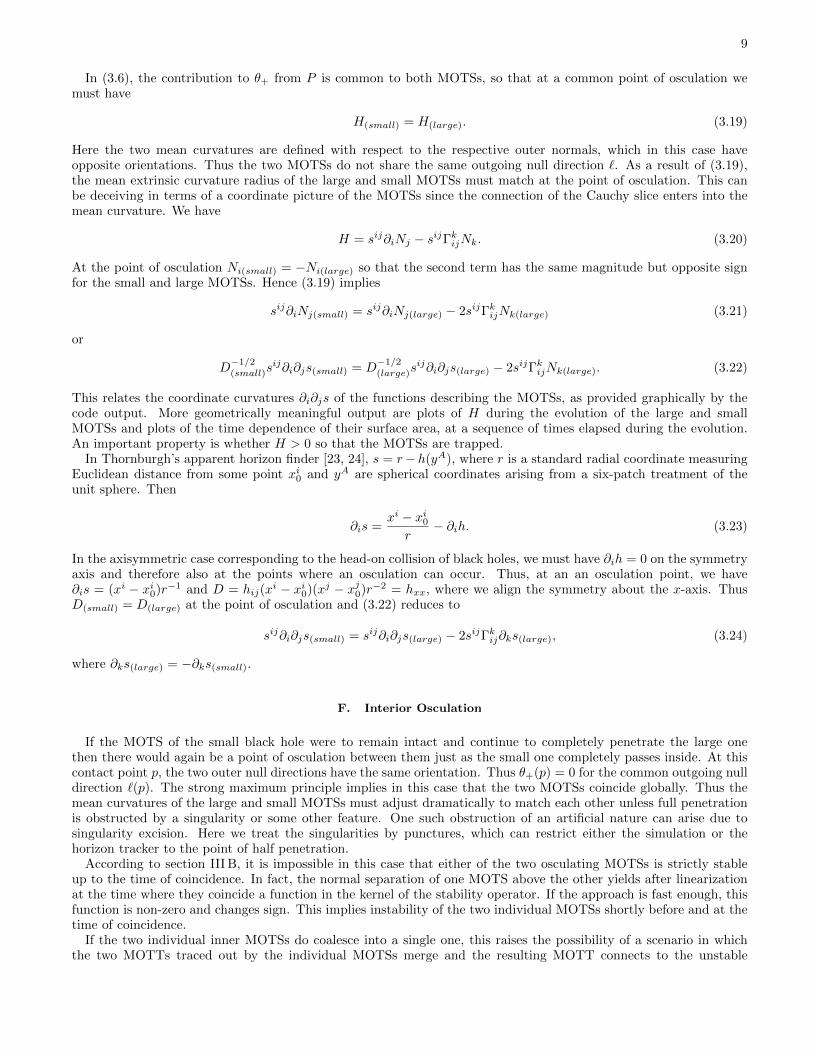
FIG. 1. A possible scenario for the evolution of the trapped tubes. The outermost MOTSs are drawn in bold. The commonoutermost MOTS develops before the first time of contact. After the separate MOTTs penetrate, the diagram illustrates thespeculative scenario that they merge and join with the unstable branch from the jump. This speculative part of the figure isindicated by the dashed part .

branch of the common horizon, whose stable branch is the MOTT traced out by the apparent horizon, as describedin section III D and depicted in Fig. 1. The figure illustrates how the two individual MOTTs can coalesce and joincontinuously to the outer apparent horizon. Although this figure looks highly suggestive, there is no reason to believethat it is actually valid. What currently is known is that there always exists an outermost MOTS, that it can jump,and that at the time of the jump there are two branches emanating from the jump target. The current state of thetheory is not able to determine how long the unstable MOTSs continue to exist. See [13] for a related discussion.

IV. SIMULATIONS

Here we present the results of the simulation of the head-on collision of two black holes with initial masses m andm/4. Besides outputting the coordinate shapes of the MOTSs detected by the horizon finder, in order to analyzetheir intrinsic geometrical structure we also output plots of the time dependence of their mean curvature H and totalarea. Since this is the first application of the harmonic code described in Sec. II, we also present convergence teststo establish validity. Convergence of the constraints is checked in the region of interest close to the MOTSs. Thisavoids the expected loss of convergence near the punctures and near the outer boundary (where constraint preservingboundary conditions have not been implemented). Because the run times necessary for the head-on collision are short,errors from the outer boundary treatment do not effect the region of interest.

A. Initial configuration of the MOTSs

We use the same time symmetric Brill-Lindquist data to initiate an axisymmetric head-on-collision as in [12], withthe exception that the black holes now have unequal masses. The conformal flatness of the initial 3-metric providesa natural choice of Euclidean coordinates (x, y, z). The initial “bare” masses of the punctures, neglecting theirinteraction, are m(large) = 4m(small) = 0.8M , corresponding to the Euclidean coordinate radii of the non-interactingblack holes r(large) = 4r(small) = 0.4M . We choose the x-axis to be the axis of symmetry, with the puncturescorresponding to the two black holes initially separated by ∆x = 1.0M . Due to their interaction at this separation,the actual masses of the individual black have ratio M(large) ≈ 3.14M(small). (See [12] for a discussion of the leadingorder effect of a finite separation on the physical parameters.) In order to avoid numerical problems, the puncturesare offset by a half grid-step from the axis of symmetry.

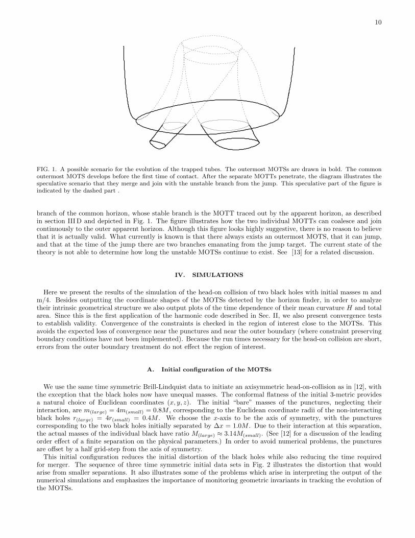
This initial configuration reduces the initial distortion of the black holes while also reducing the time requiredfor merger. The sequence of three time symmetric initial data sets in Fig. 2 illustrates the distortion that wouldarise from smaller separations. It also illustrates some of the problems which arise in interpreting the output of thenumerical simulations and emphasizes the importance of monitoring geometric invariants in tracking the evolution ofthe MOTSs.

11

−0.45 −0.30 −0.15 0.00 0.15 0.30 0.45−0.45

−0.30

−0.15

0.00

0.15

0.30

0.45

x[M

]

z [M]

FIG. 2. Cross-sections of the coordinate shapes, in units of M , of the individual MOTSs which approach each other in asequence of time-symmetric Cauchy slices. The uniqueness property of minimal surfaces keeps the MOTSs from touching andcreates considerable coordinate distortion when they are close.

At a moment of time symmetry the MOTS condition reduces to H = 0, i.e. from (3.20)

sij∂i∂js = sijΓkij∂ks. (4.1)

Then for a sequence of initial data for which the two black holes approach each other, (3.24) implies

sij∂i∂js(small) → −sij∂i∂js(large) (4.2)

at the point of closest approach. Thus if the coordinate shape of one MOTS appears convex at the point of closestapproach then the other must appear concave with the exact same magnitude of curvature. We see this effect in theinitial data sets shown in Fig 2.

Another feature of the sequence of time symmetric data sets is that the MOTSs cannot touch as their initialseparation is made smaller. This is also a consequence of the uniqueness theorem for MOTSs. In the time symmetriccase both MOTSs satisfy θ+ = θ− = 0. If they were to touch then at their common point the outer null normal toone MOTS would be the same as the inner null normal to the other. But since both null directions have vanishingexpansion, this would violate the uniqueness theorem. Note that in the time symmetric case, a MOTS is also aminimal surface so that this result also follows from the uniqueness theorem for minimal surfaces.

B. Approaching MOTSs

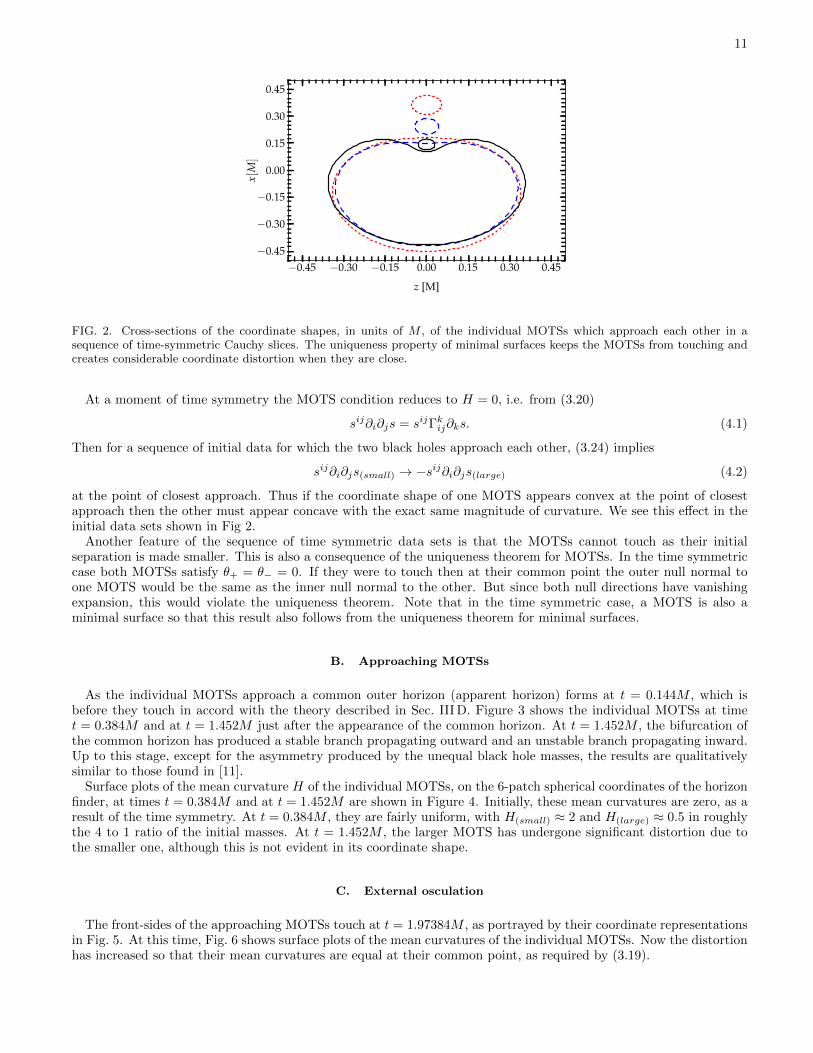
As the individual MOTSs approach a common outer horizon (apparent horizon) forms at t = 0.144M , which isbefore they touch in accord with the theory described in Sec. III D. Figure 3 shows the individual MOTSs at timet = 0.384M and at t = 1.452M just after the appearance of the common horizon. At t = 1.452M , the bifurcation ofthe common horizon has produced a stable branch propagating outward and an unstable branch propagating inward.Up to this stage, except for the asymmetry produced by the unequal black hole masses, the results are qualitativelysimilar to those found in [11].

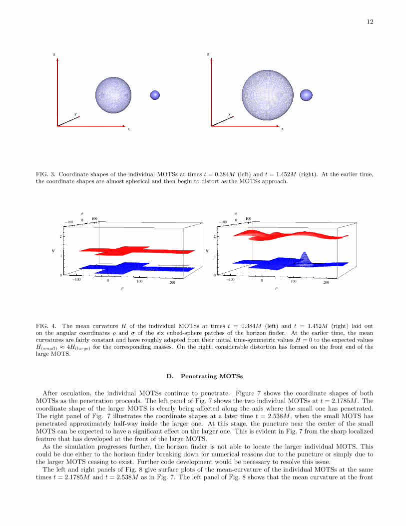
Surface plots of the mean curvature H of the individual MOTSs, on the 6-patch spherical coordinates of the horizonfinder, at times t = 0.384M and at t = 1.452M are shown in Figure 4. Initially, these mean curvatures are zero, as aresult of the time symmetry. At t = 0.384M , they are fairly uniform, with H(small) ≈ 2 and H(large) ≈ 0.5 in roughlythe 4 to 1 ratio of the initial masses. At t = 1.452M , the larger MOTS has undergone significant distortion due tothe smaller one, although this is not evident in its coordinate shape.

C. External osculation

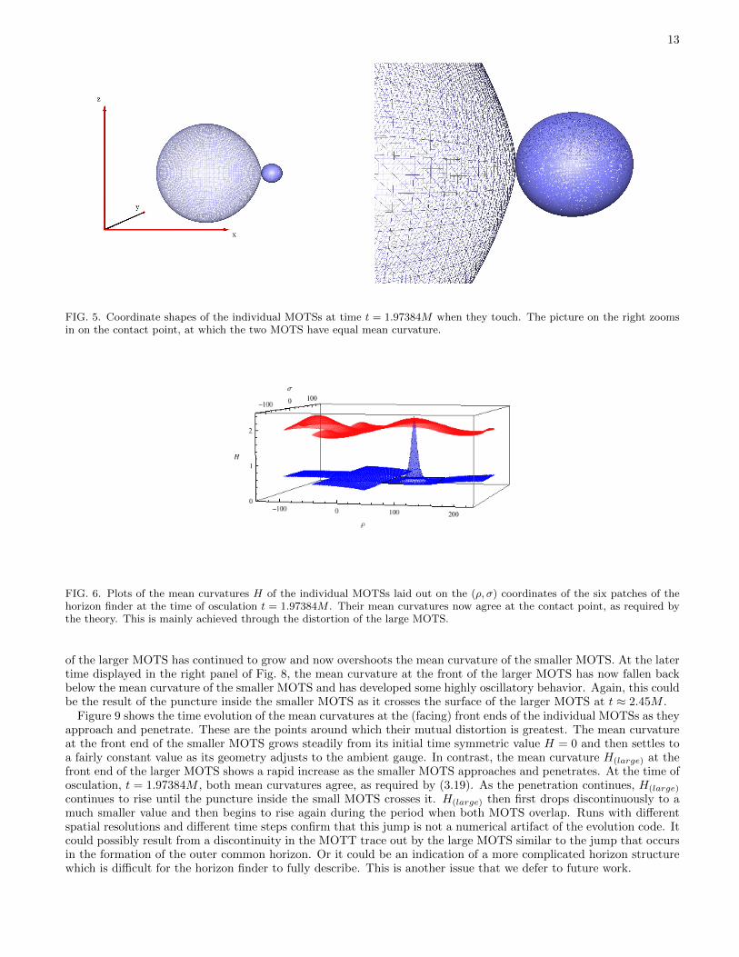
The front-sides of the approaching MOTSs touch at t = 1.97384M , as portrayed by their coordinate representationsin Fig. 5. At this time, Fig. 6 shows surface plots of the mean curvatures of the individual MOTSs. Now the distortionhas increased so that their mean curvatures are equal at their common point, as required by (3.19).

12

FIG. 3. Coordinate shapes of the individual MOTSs at times t = 0.384M (left) and t = 1.452M (right). At the earlier time,the coordinate shapes are almost spherical and then begin to distort as the MOTSs approach.

FIG. 4. The mean curvature H of the individual MOTSs at times t = 0.384M (left) and t = 1.452M (right) laid outon the angular coordinates ρ and σ of the six cubed-sphere patches of the horizon finder. At the earlier time, the meancurvatures are fairly constant and have roughly adapted from their initial time-symmetric values H = 0 to the expected valuesH(small) ≈ 4H(large) for the corresponding masses. On the right, considerable distortion has formed on the front end of thelarge MOTS.

D. Penetrating MOTSs

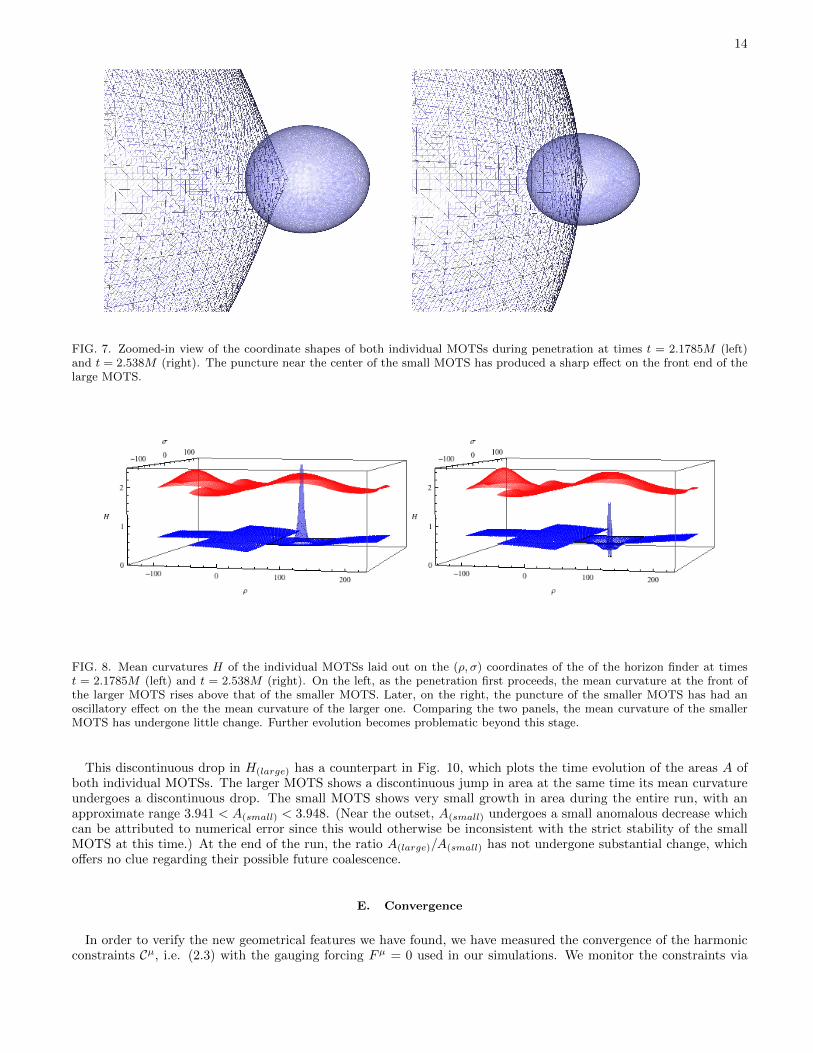
After osculation, the individual MOTSs continue to penetrate. Figure 7 shows the coordinate shapes of bothMOTSs as the penetration proceeds. The left panel of Fig. 7 shows the two individual MOTSs at t = 2.1785M . Thecoordinate shape of the larger MOTS is clearly being affected along the axis where the small one has penetrated.The right panel of Fig. 7 illustrates the coordinate shapes at a later time t = 2.538M , when the small MOTS haspenetrated approximately half-way inside the larger one. At this stage, the puncture near the center of the smallMOTS can be expected to have a significant effect on the larger one. This is evident in Fig. 7 from the sharp localizedfeature that has developed at the front of the large MOTS.

As the simulation progresses further, the horizon finder is not able to locate the larger individual MOTS. Thiscould be due either to the horizon finder breaking down for numerical reasons due to the puncture or simply due tothe larger MOTS ceasing to exist. Further code development would be necessary to resolve this issue.

The left and right panels of Fig. 8 give surface plots of the mean-curvature of the individual MOTSs at the sametimes t = 2.1785M and t = 2.538M as in Fig. 7. The left panel of Fig. 8 shows that the mean curvature at the front

13

FIG. 5. Coordinate shapes of the individual MOTSs at time t = 1.97384M when they touch. The picture on the right zoomsin on the contact point, at which the two MOTS have equal mean curvature.

FIG. 6. Plots of the mean curvatures H of the individual MOTSs laid out on the (ρ, σ) coordinates of the six patches of thehorizon finder at the time of osculation t = 1.97384M . Their mean curvatures now agree at the contact point, as required bythe theory. This is mainly achieved through the distortion of the large MOTS.

of the larger MOTS has continued to grow and now overshoots the mean curvature of the smaller MOTS. At the latertime displayed in the right panel of Fig. 8, the mean curvature at the front of the larger MOTS has now fallen backbelow the mean curvature of the smaller MOTS and has developed some highly oscillatory behavior. Again, this couldbe the result of the puncture inside the smaller MOTS as it crosses the surface of the larger MOTS at t ≈ 2.45M .

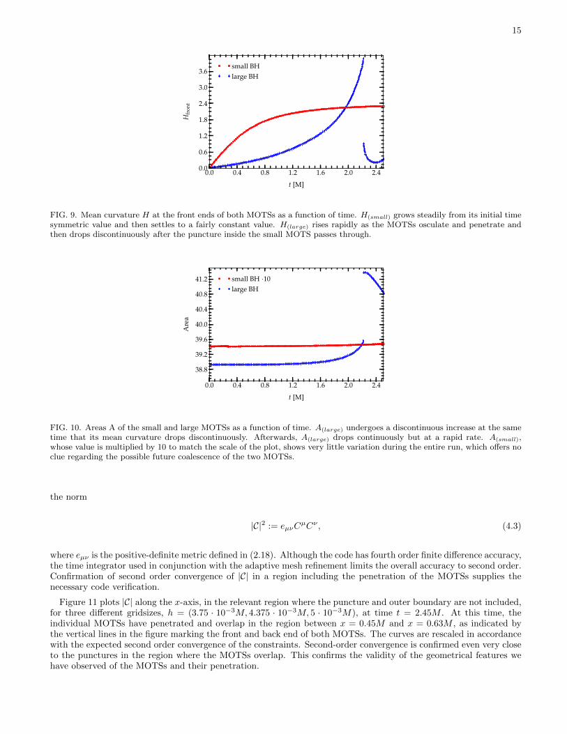
Figure 9 shows the time evolution of the mean curvatures at the (facing) front ends of the individual MOTSs as theyapproach and penetrate. These are the points around which their mutual distortion is greatest. The mean curvatureat the front end of the smaller MOTS grows steadily from its initial time symmetric value H = 0 and then settles toa fairly constant value as its geometry adjusts to the ambient gauge. In contrast, the mean curvature H(large) at thefront end of the larger MOTS shows a rapid increase as the smaller MOTS approaches and penetrates. At the time ofosculation, t = 1.97384M , both mean curvatures agree, as required by (3.19). As the penetration continues, H(large)

continues to rise until the puncture inside the small MOTS crosses it. H(large) then first drops discontinuously to amuch smaller value and then begins to rise again during the period when both MOTS overlap. Runs with differentspatial resolutions and different time steps confirm that this jump is not a numerical artifact of the evolution code. Itcould possibly result from a discontinuity in the MOTT trace out by the large MOTS similar to the jump that occursin the formation of the outer common horizon. Or it could be an indication of a more complicated horizon structurewhich is difficult for the horizon finder to fully describe. This is another issue that we defer to future work.

14

FIG. 7. Zoomed-in view of the coordinate shapes of both individual MOTSs during penetration at times t = 2.1785M (left)and t = 2.538M (right). The puncture near the center of the small MOTS has produced a sharp effect on the front end of thelarge MOTS.

FIG. 8. Mean curvatures H of the individual MOTSs laid out on the (ρ, σ) coordinates of the of the horizon finder at timest = 2.1785M (left) and t = 2.538M (right). On the left, as the penetration first proceeds, the mean curvature at the front ofthe larger MOTS rises above that of the smaller MOTS. Later, on the right, the puncture of the smaller MOTS has had anoscillatory effect on the the mean curvature of the larger one. Comparing the two panels, the mean curvature of the smallerMOTS has undergone little change. Further evolution becomes problematic beyond this stage.

This discontinuous drop in H(large) has a counterpart in Fig. 10, which plots the time evolution of the areas A ofboth individual MOTSs. The larger MOTS shows a discontinuous jump in area at the same time its mean curvatureundergoes a discontinuous drop. The small MOTS shows very small growth in area during the entire run, with anapproximate range 3.941 < A(small) < 3.948. (Near the outset, A(small) undergoes a small anomalous decrease whichcan be attributed to numerical error since this would otherwise be inconsistent with the strict stability of the smallMOTS at this time.) At the end of the run, the ratio A(large)/A(small) has not undergone substantial change, whichoffers no clue regarding their possible future coalescence.

E. Convergence

In order to verify the new geometrical features we have found, we have measured the convergence of the harmonicconstraints Cµ, i.e. (2.3) with the gauging forcing Fµ = 0 used in our simulations. We monitor the constraints via

15

0.0 0.4 0.8 1.2 1.6 2.0 2.40.0

0.6

1.2

1.8

2.4

3.0

3.6

Hfr

ont

t [M]

small BHlarge BH

FIG. 9. Mean curvature H at the front ends of both MOTSs as a function of time. H(small) grows steadily from its initial timesymmetric value and then settles to a fairly constant value. H(large) rises rapidly as the MOTSs osculate and penetrate andthen drops discontinuously after the puncture inside the small MOTS passes through.

0.0 0.4 0.8 1.2 1.6 2.0 2.4

38.8

39.2

39.6

40.0

40.4

40.8

41.2

Are

a

t [M]

small BH ·10large BH

FIG. 10. Areas A of the small and large MOTSs as a function of time. A(large) undergoes a discontinuous increase at the sametime that its mean curvature drops discontinuously. Afterwards, A(large) drops continuously but at a rapid rate. A(small),whose value is multiplied by 10 to match the scale of the plot, shows very little variation during the entire run, which offers noclue regarding the possible future coalescence of the two MOTSs.

the norm

|C|2 := eµνCµCν , (4.3)

where eµν is the positive-definite metric defined in (2.18). Although the code has fourth order finite difference accuracy,the time integrator used in conjunction with the adaptive mesh refinement limits the overall accuracy to second order.Confirmation of second order convergence of |C| in a region including the penetration of the MOTSs supplies thenecessary code verification.

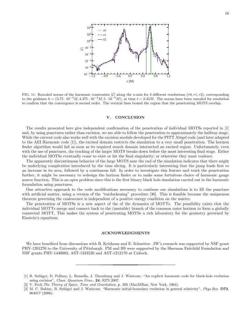
Figure 11 plots |C| along the x-axis, in the relevant region where the puncture and outer boundary are not included,for three different gridsizes, h = (3.75 · 10−3M, 4.375 · 10−3M, 5 · 10−3M), at time t = 2.45M . At this time, theindividual MOTSs have penetrated and overlap in the region between x = 0.45M and x = 0.63M , as indicated bythe vertical lines in the figure marking the front and back end of both MOTSs. The curves are rescaled in accordancewith the expected second order convergence of the constraints. Second-order convergence is confirmed even very closeto the punctures in the region where the MOTSs overlap. This confirms the validity of the geometrical features wehave observed of the MOTSs and their penetration.

16

−1.2 −0.8 −0.4 0.0 0.4 0.8 1.210−10

10−8

10−6

10−4

10−2

100

102

104

|C|

x [M]

r0r1r2

FIG. 11. Rescaled norms of the harmonic constraints |C| along the x-axis for 3 different resolutions (r0, r1, r2), correspondingto the gridsizes h = (3.75 · 10−3M, 4.375 · 10−3M, 5 · 10−3M), at time t = 2.45M . The norms have been rescaled for resolutionto confirm that the convergence is second order. The vertical lines bound the region that the penetrating MOTS overlap.

V. CONCLUSION

The results presented here give independent confirmation of the penetration of individual MOTSs reported in [1]and, by using punctures rather than excision, we are able to follow the penetration to approximately the halfway stage.While the current code also works well with the excision module developed for the PITT Abigel code (and later adaptedto the AEI Harmonic code [1]), the excised domain restricts the simulation to a very small penetration. The horizonfinder algorithm would fail as soon as its required search domain intersected an excised region. Unfortunately, evenwith the use of punctures, the tracking of the larger MOTS breaks down before the most interesting final stage. Eitherthe individual MOTSs eventually cease to exist or hit the final singularity; or otherwise they must coalesce.

The apparently discontinuous behavior of the large MOTS near the end of the simulation indicates that there mightbe underlying complexities introduced by the time slicing. It is particularly interesting that the jump leads first toan increase in its area, followed by a continuous fall. In order to investigate this feature and track the penetrationfurther, it might be necessary to redesign the horizon finder or to make some fortuitous choice of harmonic gaugesource function. This is an open problem since this is the first binary black hole simulation carried out in the harmonicformulation using punctures.

One attractive approach to the code modifications necessary to continue our simulations is to fill the puncturewith artificial matter, using a version of the “turduckening” procedure [30]. This is feasible because the uniquenesstheorem governing the coalescence is independent of a positive energy condition on the matter.

The penetration of MOTSs is a new aspect of the of the dynamics of MOTTs. The possibility exists that theindividual MOTTs merge and connect back to the (unstable) branch of the common outer horizon to form a globallyconnected MOTT, This makes the system of penetrating MOTSs a rich laboratory for the geometry governed byEinstein’s equations.

ACKNOWLEDGMENTS

We have benefited from discussions with B. Krishnan and E. Schnetter. JW’s research was supported by NSF grantPHY-1201276 to the University of Pittsburgh. PM and BS were supported by the Sherman Fairchild Foundation andNSF grants PHY-1440083, AST-1333520 and AST-1212170 at Caltech.

[1] B. Szilagyi, D. Pollney, L. Rezzolla, J. Thornburg and J. Winicour, “An explicit harmonic code for black-hole evolutionusing excision”, Class. Quantum Grav., 24, S275 2007.

[2] V. Fock,The Theory of Space, Time and Gravitation, p. 392 (MacMillan, New York, 1964).[3] M. C. Babiuc, B. Szilagyi and J. Winicour, “Harmonic initial-boundary evolution in general relativity”, Phys.Rev. D73,

064017 (2006).

17

[4] M. C. Babiuc, H.-O. Kreiss and J. Winicour, “Constraint-preserving Sommerfeld conditions for the harmonic Einsteinequations”, Phys. Rev. D75, 044002 (2007).

[5] Cactus Computational Toolkit home page: http://www.cactuscode.org.[6] S. Brandt and B. Brugmann, “A simple construction of initial data for multiple black holes”, em Phys. Rev. Lett. 78, 3606

(1997).[7] M. Alcubierre Miguel Alcubierre, B. Bruegmann, D. Pollney, E. Seidel and R. Takahashi, “Black hole excision for dynamic

black holes”, Phys.Rev. D 64, 061501 (2001).[8] S. A. Hayward, “General laws of black hole dynamics”, Phys.Rev. D 49, 6467 (1994).[9] A. Ashtekar and B. Krishnan, “Dynamical horizons and their properties”, Phys.Rev. D 68, 104030 (2003).

[10] A. Ashtekar and B. Krishnan, “Isolated and dynamical horizons and their applications”, Living Rev. Rel. 7, 10 (2004).[11] E. Schnetter and B. Krishnan, “Non-symmetric trapped surfaces in the Vaidya and Schwarzschild spacetimes”, Phys.Rev.

D 73, 021502 (2006).[12] E. Schnetter, B. Krishnan and F. Beyer, “Introduction to dynamical horizons in numerical relativity”, Phys.Rev. D 74,

024028 (2006).[13] L. Andersson, M. Mars, J. Metzger and W. Simon, “The time evolution of marginally trapped surfaces”, Class. Quantum

Grav. 26(8), 085018, 14 (2009).[14] L. Andersson, M. Mars and W. Simon, “Local existence of dynamical and trapping horizons”, Phys. Rev. Lett. 95(11),

11110 (2005).[15] L. Andersson, M. Mars and W. Simon, “Stability of marginally outer trapped surfaces and existence of marginally outer

trapped tubes”, Adv. Theor. Math. Phys. 12(4), 853–888 (2008).[16] A. Ashtekar and G. J. Galloway, “Some uniqueness results for dynamical horizons”, Adv. Theor. Math. Phys. 9(1), 1–30

(2005).[17] H. Friedrich and A. Rendall, “The Cauchy Problem”, in Einstein’s Field Equations and their Physical Interpre-

tation, ed. B. G Schmidt (Springer-Verlag, Berlin, 2000).[18] H. Friedrich, “Hyperbolic reductions for Einstein’s equations.“ Class. Quantum Grav. 13 1451-1469, (1996)[19] P. Mosta, ”Puncture Evolutions within the Harmonic Framework”, Diploma thesis, Universitat Kassel (2008).[20] H.-O. Kreiss, O. Reula, O. Sarbach, and J. Winicour, “Boundary conditions for coupled quasilinear wave equations with

application to isolated systems”, Commun.Math.Phys. 289, 1099 (2009)[21] E. Schnetter, S. H. Hawley and I. Hawke, “Evolutions in 3D numerical relativity using fixed mesh refinement”, Class.

Qunatum Grav. 21, 1465 (2004).[22] “Mesh refinement with Carpet”, http://www.carpet.code.org.[23] J. Thornburgh, “Finding apparent horizons in numerical relativity”, Phys. Rev. D 54, 4899 (1996).[24] J. Thornburgh, “A fast apparent-horizon finder for 3-dimensional Cartesian grids in numerical relativity”, Class. Quantum

Grav. 21, 743 (2004).[25] L. Andersson and J. Metzger, “The area of horizons and the trapped region”, Comm. Math. Phys. 290(3), 941–972 (2009).[26] M. Eichmair, “The plateau problem for marginally outer trapped surfaces”, J. Differential Geom. 83, 551-584 (2009).[27] M. Eichmair, “Existence, regularity, and properties of generalized apparent horizons”, Commun. Math. Phys. 294, 745-760

(2010).[28] L. Andersson and J. Metzger, “Curvature estimates for stable marginally trapped surfaces”, J. Differential Geom. 84,

231-265 (2010).[29] G. J. Galloway, “Rigidity of marginally trapped surfaces and the topology of black holes”, Comm. Anal. Geom. 16(1),

217–229 (2008).[30] D. Brown, P. Diener, O. Sarbach, E. Schnetter and M. Tiglio, “Turduckening black holes: an analytical and computational

study”, Phys. Rev. D 79, 044023 (2009).