i-h'ai October 1988 · October 1988 I& - !&W APPLICATIONS OF CATASTROPHE THEORY Synectics Corporation DTIC AME ECTh=ra A.E.R. Woodcock, L. Cobb, M.E. Familant, J. Markey S 2i89 -APPROVED

RADC-TR-88-212i-h'ai Technical ReportOctober 1988

I&- !&W APPLICATIONS OF CATASTROPHE

THEORY

Synectics Corporation DTICAME ECTh=ra

A.E.R. Woodcock, L. Cobb, M.E. Familant, J. Markey S 2i89 -

APPROVED FOR PUBLIC RELEASE; DISTRIBUTION UNLIMITED.

This effort was funded totally by the Laboratory Director's fund.

ROME AIR DEVELOPMENT CENTERAir Force Systems Command

Griffiss Air Force Base, NY 13441-5700

389 24

UNCLASSIFIEDECUITY CLASIFIAMON OF TMI PAGE

Form AoprovedREPORT DOCUMENTATION PAGE OMB No. 0704-IM

Ig. REPORT SECURITY CLASSIFICATION lb. RESTRICTIVE MARKINGSUNCLASSIFIED MIA

2a. SECURITY CLASSIFICATION AUTHORITY 3. DISTRIBUTION/AVAILABIUTY OF REPORTNIA Approved for public release;

/b. DECLASSIFICATION DOWNGRADING SCHEDULE distribution unlimited.4. PERORMING ORGANZATION REPORT NUMER(S) ' S. MONITORING ORGANIZATION REPORT NUMBER(S)

WH-86-LQ-00 RADC-TR-88-212

Go. NAME OF PERFORMING ORGANIZATION 6b. OFFICE SYMBOL 7a. NAME OF MONITORING ORGANIZATION

Synectics Corporation f Rome Air Development Center (IRDW)

6C. ADDRESS (Otj State, a ZIP Code) 7b. ADDRESS (City, State, and ZIP Cod)111 East Chestnut Street Criffiss AFB NY 134!-5700Rome NY 13440

8a, NAME OF FUNDINGISPONSORING 8b. OFFICE SYMBOL 9. PROCUREMENT INSTRUMENT IDENTIFICATION NUMBERORGANIZAON (if a . F30602-87-C-0054Rome Air Development Center ID

6c. ADDRESS (CIMt, Stte, and ZIP Code) 10. SOURCE OF FUNDING NUMBERSPROGRAM PROJECT TASK WORK UNIT

Griffiss AFB NY 13441-5700 ELEMENT NO. NO. NO. ACCESSION NO.61101F LDFP 02 C7

11. TITLE (include Sewfty Classiffeon)

I&W APPLICATIONS OF CATASTROPHE THEORY .... '.. I . !.

12. PERSONAL AUThOR)A.E.R. Woodcock, L. Cobb, M.E. Familant, 3. Markey

13a. TYPE OF REPORT 13b. TIME COVERED 14. DATE OF REPORT (Year, MAnth, Day) IS. PAGE COUNTFinal FROM May 87 TOVa 8 October 1988 214

16. SUPPLEMENTARY NOTATION

This effort was funded totally by the Laboratory Director's fund.

17. CUSATI CODES 18. SUIJECT TERMS (Contine on reverse if necenay and identify by block number)FIELD GROUP SUB-GROUP Catastrophe Theory, Indications and Warning, Non-linear

12 04 Mthematice

9. ABSTRACT (Cobuan rew Ivecrn a A.d i.f by block .o- "Mathematical and statistical tools based on catastrophe theory have been developed and imple-

mented as a fully functional oftware system which permits the capturing of data derived fromanalyst's perceptions of GW-related data elements end their analysis with a computer programbased on statistical catastrophe theory. This system permits individuals with no mathe-matical background to undertake a rigorous analysis on non-linear I&W-related and otherphenomena. These tools have been used in experiments with intelligence analysts involvingthe simulated detection of GMe, one of the most difficult problems of tactical analysis. Aset of unclassified notional indicators predicting the development of an OGG was developedand ten specific settings of these indicators were presented to intelligence analysts whowere asked to assess the probability of OMG development. The resulting assessments werecaptured and analyzed and this revealed the existence of perceptual ambiguity as well as thepotential for sudden and gradual perceptual changes, perceptual hysteresis, and perceptual

trpig (Continued)

20. DISTRIBUTION I AVAILABIUTY OF ABSTRACT 21. ABSTRACT SECURITY CLASSIFICATIONJ2UNCLASSIFIEDAJNLtMITED E3 SAME AS RPT. C) DT1C USERS IUNCLASSIFIED

22a. NAME OF RESPONSIBLE INDIVIDUAL 22b. TELEPHONE (Include Area Code) 22c. OFFICE SYMBOLPatricia M. Langendorf (315) 330-3126 RADC (IRDW)

DO Form 1473, JUN 86 Previos lomr art obsolete. SECURITY CASSIFICATION OF THIS PAGEUNCLASSIFIED

UNCLASSIFIED

Block 19 (Continued)

The experienced Intelligence analysts who served as subjects had no mathematical background,yet were enthusiastic about the technology. They were particularly Interested n aperceived capability to analyse themselves and to identify and correct inconsistentand ambiguous responses. This research has provided evidence that I&W indicators areneither linear nor uncorrelated in the mind of experienced intelligence analysts, afinding which is itself of value. The technology is directly applicable to communicatinganalyst understanding to battlefield commanders, and to capturing ambiguities in battle-field commander's perception of the combat environment. The technology also appears to beof value as an aid to intelligence analysts and decision-makers since it providesfacilities for:

1. Alerting individuals to conditions where small changes in indicator input can giverise to either gradual or sudden changes of perception in the same situation underdifferent conditions.

2. Kaking available an analytic capability that can give rational interpretations ofnon-linear and apparently counter-intuitive behavior and for clarifying the causesand effects of ambiguous perceptions.

3. Identifying and characterizing the different types of responses of intelligenceanalysts and others to features of I&W-related data sets and providing methods thatcan be used to support the training of such analysts and the interpretation ofthei- assessments of particular sets of indicators.

This technology provides a method for developing a new understanding of the non-linearaspects of the military analytic process. This understanding can be extended from theintelligence analysis of HGCs to the command and control (C2 ) arena by providing newmethods for identifying and selecting particular responses from a list of response optionsavailable to the commander. Such a facility is of obvious importance to C2 , and is beinginvestigated.

UNCLASSIFIED

ACKNOWLEGEMENTS

Dr. Woodcock would like to thank Ms. Patricia Langendorf, RADC Intelligence andReconnaissance Directorate, Rome Air Development Center, Griffiss Air Force Base, IWCATCOTR, for her continuing interest in and support of the IWCAT project.

Dr. Woodcock is very grateful to Dr. Frederick Diamond, Chief Scientist, RADC, for hissupport of and interest in the IWCAT effort.

Dr. Woodcock would like to acknowledge the participation in the LWCAT project of Dr.Loren Cobb, Medical University of South Carolina, Charleston, South Carolina, particularlyfor his work in providing a new version of the Cusp Surface Analysis program. Dr.Woodcock would also like to acknowledge the participation of Dr. M. Elliott Familant, Mr.John Markey, Mr. Wayne Worthington, Mr. Tony DePace, and Mr. Greg Howard (SynecticsCorporation) in the IWCAT project.

Dr. Woodcock would like to thank Ms. Dorothea Martin for the proof reading andproduction of this document.

Accesion For

NTIS CRA,&r

U ,,- ....:: . .

.. .T ''y {L(des

SA .j' I or

i ~'i

EXECUTIVE SUMMARY

This is the final technical report for the "I&W Applications of Catastrophe Theory(IWCAT)" project performed by Synectics Corporation (Dr. A. E. R. Woodcock, ProjectDirector and Chief Scientist) for The Rome Air Development Center (RADC) (Ms. P.Langendorf, COTR), Contract Number: F30602-87-C-0054. The IWCAT effort has provideda successful demonstration of the use of catastrophe theory to analyze indications and warning(I&W)-related data and has provided new insights to the process of the analysis and under-standing of military indicators, particularly in the area of Operational Maneuver Groups(OMGs).

Mathematical and statistical tools based on catastrophe theory have been developed andimplemented as a fully functional software system which permits the capturing of data derivedfrom analyst's perceptions of OMG-related data elements and their analysis with a computerprogram based on statistical catastrophe theory. This system permits individuals with nomatherr.atical background to undertake a rigorous analysis of non-linear I&W-related and otherphenomena. These tools have been used in experiments with intelligence analysts involvingthe simulated detection of OMGs, one of the most difficult problems of tactical analysis. A setof unclassified notional indicators predicting the development of an OMG was developed andten specific settings of these indicators were presented to intelligence analysts who were askedto assess the probability of OMG development. The resulting assessments were captured andanalyzed and this revealed the existence of perceptual ambiguity as well as the potential forsudden and gradual perceptual changes, perceptual hysteresis, and perceptual trapping.

The experienced intelligence analysts who served as subjects had no mathematical back-ground, yet were enthusiastic about the technology. They were particularly interested in aperceived capability to analyze themselves and to identify and correct inconsistent andambiguous responses. This research has provided evidence that I&W indicators are neitherlinear nor uncorrelated in the mind of experienced intelligence analysts, a finding which is itselfof value. The technology is directly applicable to communicating analyst understanding tobattlefield commanders, and to capturing ambiguities in battlefield commander's perception ofthe combat environment. The technology also appears to be of value as an aid to intelligenceanalysts and decision-makers since it provides facilities for:

1. Alerting individuals to conditions where small changes in indicator input can give riseto either gradual or sudden changes of perception in the same situation under differentconditions.

2. Making available an analytic capability that can give rational interpretations of non-linear and apparently counter-intuitive behavior and for clarifying the causes andeffects of ambiguous perceptions.

3. Identifying and characterizing the different types of responses of intelligence analystsand others to features of I&W-related data sets and providing methods that can beused to support the training of such analysts and the interpretation of their assess-rments of particular sets of indicators.

This technology provides a method for developing a new undtrstanding of the non-linear aspects of the military analytic process. This understanding can be extended from theintelligence analysis of OMGs to the command and control (C2) arena by providing newmethods for identifying and selecting particular responses from a list of response optionsavailable to the commander. Such a facility is of obvious importance to C2, and is beinginvestigated.

iii

TABLE OF CONTENTS

SECTION 1. IWA RJETRVE 1-1

1.1 The AWCAT Effort in Context------------ 1-11.2 Catastrophe Theory can Provide New Tools for the I&W Analyst ---- 1.21.3 Operational Maneuver Group Characteristics - -------------------- 1-51.4 IWCAT Concept of Operations ---------------------------------- 1-6

1.4.1 Mapping I&W Problems to Catastrophe Theory Surfaces ---- 1-61.4.2 A Catastrophe Theory-Based Knowledge Development

Environment -- ----------------------------------------- 1-81.4.2.1 Test Data Sets--------------------------------------- 1-101.4.2.2 The Collection of Test Assessments -------------------- 1-111.4.2.3 The Processing of 0MG Assessment Data----------------- 1-11

1.5 Cusp Surface Analysis ------- ------- - --- 1-15

1.5.1 Estimating Parameters --------------------------------- 1-151.5.2 Making Predictions ----------------------------------------- 1-15

1.6 OMG Threat Assessment Analyses -- ------- ---- 1-20

1.6.1 Mapping Data to the Catastrophe Modcd Surface ---------- 1-201.6.2 Specific Analyst Assessments ------------------------- 1-241.6.2.1 The Perceptions of "Analyst A"- -- 1-33

SECTION 2. THE IWCAT EFFORT IN CONTEXT -------------------- ------ 2-1

2.1 New Facilities are Needed to Support the I&W Analyst--------------- 2-12.2 Activities of I&W Intelligence Analysts------------------------------2-22.3 Operational Maneuver Group Characteristics -- --------------- 2-4

2.3.1 OMGs and Other Militay Units - -------------------- 2-52.3.2 Identifying OMGs ------ -------------------- ----------- 2-52.3.2.1 Time and Location of 0MG Insertion-------------------- 2-52.3.2.2 Concomitant Activity of Other Military Units---------------2-52.3.2.3 Changes to Military Units Becoming OMGs --------------- 2-6

2.4 Catastrophe Theory can Provide New Tools for the I&W Analyst ---- 2-72.5 Models of Perception can be Based on Catastrophe Theory------------ 2-8

2.5.1 Sudden Changes in Perception -------------------------- 2-112.5.2 Divergence - ----------- ---- ------- -------------- 2-112.5.3 Bimnodality -------------------------------------------- 2-l12.5.4 Hysteresis ------------------------------------------ 2-11

iv

TABLE OF CONTENTS (Continued)

SECTION 3. IWCAT CONCEPT OF OPERATIONS - ----- ----- 3-1

3.1 Overview 3-13.2 Mapping I&W Problems to Catastrophe Theory Surfaces ----...------ 3-3

3.2.1 Single- Valued and Multi-Valued Functions 3-4

3.2.2 Singly Stable and Bi-Stable Perceptions ---........--------.-- 3-4

3.3 A Catastrophe Theory-Based Knowledge Development Environment -- 3-9

3.3.1 The 0MG Indications and Warnings Problem ---......----------- 3-103.3.2 The Source Evaluation System ---------------....------- 3-103.3.3 The Test Data Sets ----...................----------------- --- 3-113.3.3.1 Number of Active Indicators --------- ---------- 3-133.3.3.2 Level of Confidence ---------------------------------------------- 3-153.3.3.3 Scenario Presentation -----.....................----------------- 3-153.3.3.4 Sample Sequences ----------- .................--------------------- 3-193.3.4 The Collection of Test Assessments -----........------- 3-243.3.5 The Processing of OMG Assessment Data 3-24

SECTION 4. CUSP SURFACE ANALYSIS ----------- --------- 4-1

4.1 Preliminary Notes on Terminology ----------------- 4-14.2 Introduction -- - - ------------..-------------..........------- 4-14.3 Estimating the Parameters ---....................----------------------- 4-64.4 Testing the Model -------.......-------------------....---- ----- 4-74.5 Making Predictions -.-------- .........................------------------------ 4-124.6 A Sample Output --------.-.-- .....................-------------------------- 4-14

SECTION 5. USING THE IWCAT SYSTEM ----------------............--- ---- 5-1

5.1 Statistical Analysis and Catastrophe Theory --------- .....---------------- 5-1

5.1.1 Key Variables -...-.------ ...--..............--------------------- 5-1

5.2 System Requirements ------------ ----------- 5-2

5.2.1 Hardware ----------------..................--------------------------- 5-25.2.2 Software ---...----------....................-------------------------- 5-25.2.3 Getting Started ---.-..................---------------.--------------- 5-2

5.3 The IWCAT System --------------------------------------------------------- 5-3

5.3.1 Menu Display Overview ----------- ............ - ------------------ 5-35.3.2 Read About the Program ------.....................---------------- 5-35.3.3 Enter Information About Yourself -------------------------------- 5-65.3.4 Make a Test File -........................--------------------.-.-- 5-65.3.5 Practice Session -.-.------ .....................---------------------- 5-105.3.5.1 Practice Data Presentation ------------------------------.----- 5-105.3.5.2 Practice OMG Threat Assessment --------------...-------- 5-15

v

TABLE OF CONTENTS (Continued)

5.3.6 Take the Test ----------------------------- 5-155.3.6.1 Test Data Presentation ----.................----------.--------- 5-155.3.6.2 0MG Threat Assessmnt ------.......------------------------- 5-195.3.7 Make aFile for Analysis ------- -------- 5-19

5.3.8 Perform Cusp Analysis ----------- ...---------------.--------- 5-235.3.8.1 Testing the Model -------------------------------------.. .. 5-285.3.8.2 Making Predictions ------------- ------------- 5-355.3.9 Termination of Analytic Session 5-35

SECTION 6. OMG THREAT ASSESSMENT ANALYSIS ------------------------- 6-1

6.1 Statistical Analysis of the OMG Threat Assessment Data Base --------- 6-1

6.1.1 Mapping Data to the Catastrophe Model Surface ---------------- 6-36.1.2 Sudden and Gradual Perceptual Changes -.........------------ 6-66.1.3 Divergence ---------.-.-------.- ............----------- --- - ----- 6-66.1.4 Ambiguity -.----- ...- ..--...............-------------------------- 6-66.1.5 "Slicing" the Cusp Surface ---------..............-------------- 6-66.1.6 Perceptual Hysteresis -....................----------------------- 6-116.1.7 Perceptual "Trapping" ... -----------------------------------... 6-116.1.8 Counter-Intuitive or Paradoxical Behavior -----............. --- 6-15

6.2 Specific Analyst Assessments 6-15

6.2.1 "Analyst A" ------------------- ---- 6-176.2.2 "Analyst B" -------- ------------ 6-246.2.3 "Analyst C" ------------------- ..............--------------------- 6-306.2.4 "Analyst D" ---------------------.........---------------------- 6-356.2.5 "Analyst E" --.................................--------------------- 6-37

APPENDIX A: AN OVERVIEW OF CATASTROPHE THEORY ------------.----- A-1

A. 1 Catastrophe Theory - A Proven Framework -..............------------- A-1A.2 The Properties of the Cusp Catastrophe --------- ------- A-3A.3 The Properties of the Butterfly Catastrophe ---......-----------... A-6A.4 Catastrophe Theory-Based Models of Military Behavior --....---------- A-6

A.4.1 A Cusp-Catastrophe-Based Model ------- A-6A.4.2 A Butterfly-Catastrophe-Based Model ---------------------------- A-8

APPENDIX B: BIBLIOGRAPHY --------.....................----------.------------ B-1

vi

LIST OF EXHIBITS

1-1 Catastrophe Theory-Based I&W Assessment Activities -------- ----- 1-4

1-2 Overview of the IWCAT Concept of Operations 1-71-3 Components of the IWCAT Analyst Computer Display ---------....... ----- 1-91-4 Analyst OMG Threat Assessment and Data Base Formation Activities ------- 1-121-5 Relationship of the OMG Threat Assessment Data Base to the Cusp

Catastrophe Manifold Control Plane -----.......................--------------- 1-131-6 Fitting OMG Threat Assessment Data Base to the Cusp Manifold Surface ---- 1-14

1-7 A Conventional or a Catastrophe Theory-Based Approach? --------- 1-171-8 Criteria for Acceptance of the Cusp Catastrophe-Based Model ------------ 1-181-9 Cusp Surface Analysis: Making Predictions ---------------...------------------ 1-191-10 IWCAT System Activities -------------........................---------------- 1-211-11 I&W Analyst-Derived Data Plotted on the Control Plane of the Cusp Model-- 1-221-12 Mapping Data to the Cusp Model Surface -------- ...----------------------.. 1-231-13 Cusp Model of Sudder and Gradual Changes in Analyst Perceptions ------- 1-251-14 Cusp Model of Divergent Perceptions ----------...............------------- 1-261-15 Cusp Model Can Provide a New Understanding of the Causes of

Perceptual Ambiguity ---------------------------- 1-271-16 "Slicing" the Cusp Surface ----------------------------------- ---------------------- 1-281-17 Perceptual Hysteresis ----.- ..........................--------..------------------ 1-291-18 Partial Perceptual "Trapping" ....................--------------------------------- 1-301-19 Complete Perceptual "Trapping" .....................----------..--------------- 1-311-20 Counter-Intuitive or Paradoxical Behavior ----....................------------- 1-321-21 Analysis of OMG Threat Assessment Data 1-341-22 Analysis of OMG Threat Assessment Data ------ ------------- 1-351-23 Analysis of OMG Threat Assessment Data ------------ ----- 1-371-24 Analysis of OMG Threat Assessment Data --------------------------------------- 1-381-25 Analysis of 0MG Threat Assessment Data ---....................------------- 1-392-1 IWCAT Environment --------------------------------------------------------------- 2-32-2 Input Characteristics ---------------------- -------------------------------- 2-92-3 Increasing Detail -.-...------....................-----------..----------------- 2-102-4 Sudden Changes -.....---------.-.-...............-----..------------.------- 2-122-5 The Property of Divergence --......................------------------ ------ 2-132-6 The Property of Bimodality ---.................---------..------------- - ---- 2-142-7 Perceptions Can Exhibit Hysteresis ---------------------------------------------- 2-15

vii

LIST OF EXHIBITS (Continued)

3-1 Overview of the IWCAT Concept of Operations -------------- 3-2

3-2 Functional Relationships -------------------------------- 3-5

3-3 Singly-Stable and Bi-Stable Perceptions 3-6

3-4 Catastrophe Theory-Based I&W Assessment Activities 3-8

3-5 The "Source Evaluation System" 3-12

3-6 Selected I&W-Related Indicators --------------------- 3-14

3-7 Indicator Activity Patterns as a Function of Number of Active Indicators --- 3-16

3-8 Components of the IWCAT Analyst Computer Display ---------- 3-17

3-9 Analyst OMG Threat Assessment and Data Base Formation Activities ------- 3-20

3-10 Relationship of the OMG Threat Assessment Data Base to the Cusp

Catastrophe Control Plane --...-.-.-- ................---..-------.------------ 3-26

3-11 Fitting the OMG Threat Assessment Data Base to the Cusp

Catastrophe Manifold 3-27

4-1 The Linear Model Used by Multiple Regression -..............------------- 4-2

4-2 The Cusp Catastrophe Model ------- ----------------------- 4-4

4-3 Sections Through the Cusp Catastrophe Model ------- --------- 4-5

4-4 The Type N 3 PDF for the Cusp Catastrophe Model -------.....-------- 4-8

4-5 A Conventional or a Catastrophe Theory-Based Approach? ........ -; --------- 4-9

4-6 Criteria for Acceptance of the Cusp Catastrophe-Based Model ---------------- 4-11

4-7 Cusp Surface Analysis: Making Predictions ------------------ 4-13

4-8 The Effect of Linear Factors 4-15

4-9 Sample Output from the Cusp Surface Analysis Program ------- --- 4-16

5-1 IWCAT System Overview Menu Display 5-4

5-2 IWCAT System Overview Menu Display, Option 1: Read About

the Program--------------- ----- 5-5

5-3 IWCAT System Overview Menu Display, Option 2: Enter

Information About Yourself -----...------....................----------- - .-- 5-7

5-4 IWCAT System Overview Menu Display, Option 3: Make a Test File ------ 5-8

5-5 Making a Test File -------.-.- .......................---------- ------------------ 5-9

5-6 IWCAT System Overview Menu Display, Option 4: Practice Session ------- 5-11

5-7 Entering OMG Assessment Practice Data -------------..------.----- 5-12

5-8 Practice Session Activities -.-......................-----------.--------------- 5-13

5-9 Practice Data Display ---------------------- 5-14

viii

LIST OF EXHIBITS (Continued)

5-10 IWCAT System Overview Menu Display, Option 5: Take the Test -------- 5-165-11 Enter OMG Test Data Assessments ----------- 5-175-12 OMG Test Data Presentation 5-185-13 OMG Threat Assessment Activities 5-205-14 IWCAT System Overview Menu Display, Option 6: Make a File

for Analysis 5-21

5-15 Making a File for Statistical Analysis ------------------------ --------------------- 5-225-16 IWCAT System Overview Menu Display, Option 7: Perform Cusp

Analysis -...---- ...-.-...-..-.-...-.-....------------------------------------- 5-245-17 Cusp Analysis Activities ------------------------------ -------......--------------- 5-2-,5-18 Sample Output from the Cusp Surface An -lysis Program ------- ------- 5-275-19 Sample Output from the Cusp Surface Analysis Program --------------------- 5-295-20 Sample Output from the Cusp Surface Analysis Program 5-305-21 Sample Output from the Cusp Surface Analysis Program --------------------- 5-315-22 Sample Output from the Cusp Surface Analysis Program ------- 5-325-23 Sample Output from the Cusp Surface Analysis Program 5-335-24 Sample Output from the Cusp Surface Analysis Program ----...----------- 5-346-1 IWCAT System Activities ----------------................-------------------------- 6-26-2 I&W Analyst-Derived Data Plotted on the Control Plane of the Cusp Model - 6-46-3 Mapping Data to the Cusp Model Surface ---------------------------------- 6-56-4 Cusp Model of Sudden and Gradual Changes in Analyst Perceptions ------- 6-76-5 Cusp Model of Divergent Perceptions ---------.................-------- 6-86-6 Cusp Model Can Provide a New Understanding of the Causes of

Perceptual Ambiguity 6-96-7 "Slicing" the Cusp Surface -.......................---..----------------------- 6-106-8 Perceptual Hysteresis -.......................-------- ................---------- 6126-9 Partial Perceptual "Trapping" ------------------------------------------------------- 6-136-10 Complete Perceptual "Trapping" ........................------------------------ 6-146-11 Counter-Intuitive or Paradoxical Behavior -...................----------------- 6-166-12 Analysis of OMG Threat Assessment Data --------------------------------------- 6-18

6-13 Analysis of OMG Threat Assessment Data -..................----------------- 6-20

6-14 Analysis of OMG Threat Assessment Data -...............-------------.. 6-226-15 Analysis of OMG Threat Assessment Data -----............------------ 6-23

ix

LIST OF EXHIBITS (Contiiued)

6-16 Analysis of OMG Threat Assessment Data -..................------------.--- 6-25

6-17 Analysis of OMG Threat Assessment Data --------------------- 6-27

6-18 Analysis of OMG Threat Assessment Data 6-29




6-22 Analysis of OMG Threat Assessinent Data ------------------ 6-36

A-1 The Elementary Catastrophes A-2

A-2 The Cusp Catastrophe Function VCC(x) -.....................---------------- A-4

A-3 The Cusp Catastrophe Manifold and Control Plane ---------------- A-5

A-4 The Butterfly Catastrophe Potential Function VBC(x) and Manifold -------- A-7

A-5 A Military Analysis and Problem-Solving Landscape --------- ----- A-9

A-6 Application of Catastrophe Theory to Military Analysis ------------- A-10

A-7 A Military Analysis and Problem-Solving Landscape ----- A-11

x

SECTION 1. WCAT PROJECT REVIEW

This is the final technical report for the "I&W Applications of Catastrophe Theory(1WCAT)" project performed by Synectics Corporation (Dr. A. E. R. Woodcock, ProjectDirector and Chief Scientist) for The Rome Air Development Center (RADC) (Ms. P.Langendorf, COTR).

The IWCAT effort has provided a successful demonstration of the use of catastrophetheory to analyze indications and warning (I&W)-related data and has provided new insights tothe process of the analysis and understanding of military indicators, particularly in the area ofOperational Maneuver Groups. Methods have been made available which can serve to identifyconditions under which sudden and gradual changes, divergence, ambiguities, paradoxicalreversals, hysteresis, and perceptual "trapping" can take place and can aid in assessing theirimpact on the interpretation of the data.

A fully functional IWCAT software system has been developed which permits thecapturing of data derived from analyst's perceptions of 0MG-related data elements and theiranalysis with a computer program based on statistical catastrophe theory. This system couldserve as the basis of a fully operational I&W facility which is sensitive to nonlinear changes inperception, a capability which cannot be provided by systems which use linear regressiontechniques for analysis.

Several members of Synectics staff who have been involved in various forms of I&Wand intelligence analysis activity participated in testing the IWCAT system as it nearedcompletion. Information generated by this process was then subjected to analysis using thecusp analysis program. It is a suggestive finding of this statistical analyses performed duringthis investigation that the nature of the response of the different analysts to the OMG threat testdata appeared to depend upon their background and experience. The suggestions of analystbackground- and experience response-specificity is a tentative finding due to the small samplesize of analysts that were used in the experiment. However, such a suggestion can haveprofound implications on the way that I&W and other forms of intelligence analyses areperformed. These possibilities should be the subject of further analytic activities andinvestigations with the aid of the IWCAT system which can form the basis of a test-bed forsuch a study.

1.1 THE IWCAT EFFORT IN CONTEXT

The I&W Applications of Catastrophe Theory (IWCAT) effort has determined that it isfeasible to use catastrophe theory and related mathematical techniques to provide new facilitiesto support the activities of I&W analysts in areas of importance to the Air Force. Investigationshave concentrated on the use of indicators related to the formation of Operational ManeuverGroups (OMGs) as a test of the system This effort has involved the development of a newflexible and adaptable problem-solvir - and decision-making environment that is able to captureand use small, and apparently insignificant, changes in information that are the precursors ofdramatic changes in overall system behavior.

This final technical report identifies OMG detection as the specific I&W-related problemwhich is amenable to analysis with the techniques of applied catastrophe theory. In general,suitable I&W problems for such analysis will be those in which several key influencesdetermine system behavior and which exhibit some or all of the following properties:

1-1

1. Gradual and sudden changes, divergence, bimodality, and hysteresis that arecharacteristic of the behavior exhibited by the elementary catastrophes.

2. Small changes in the information (provided to an I&W analyst, for example) can give

rise to either small or large changes in perception under the same conditions.

3. Small biases in information can give rise to dramatically different analytic results.

After extensive discussions with the government, the IWCAT team selected an I&Wproblem which involved the recognition of an OMG, one of the most difficult problems intactical analyses, as a test problem. A set of ten indicators predicting the development of aSoviet OMG was developed. Settings of these indicators were presented to military analystswho were asked to assess the probability of 0MG development. These assessments werecaptured and analyzed with the aid of a statistical program based on catastrophe theory.

1.2 CATASTROPHE THEORY CAN PROVIDE NEW TOOLSFOR THE I&W ANALYST

Recent advances in mathematics in such areas as catastrophe theory have provided a newunderstanding of the nature of highly complicated and inherently nonlinear systems. Theseadvances have paved the way for the application of new mathematical techniques to suchproblems as those associated with I&W. These applications can be supported through thedevelopment and use of new analytic "tools" based upon catastrophe theory. However, inorder to avoid prohibitively long training periods, such tools should be made available to I&Wanalysts and decision-makers in such a way that these individuals are not required to under-stand their mathematical details. The IWCAT system has achieved such "mathematical trans-parency" through the use of menus, other forms of man-machine interface techniques, andself-documentation by means of appropriate text files.

Military analysts and decision-makers in the indications and warning (I&W) area arefaced with the need to analyze and understand large amounts of often conflicting and contra-dictory data derived from sensors, communications systems, and other sources. These tasksoften have to be performed under severe time-pressure and if used in the field, at some actualphysical risk to the analysts and decision-makers themselves. Faced with the problem ofinformation overload in critical periods of combat, such individuals will have to resort to theuse of analytic methods that capture the essence of system behavior and "friendly" graphicsdevices that can facilitate the understanding, reasoning, and decision-making activities ofanalysts in ways that develop and reinforce their perceptions. The IWCAT effort has produceda prototype computer-based system that can support the I&W analyst by providing a newtechnology for capturing I&W analysts' perceptions of situations of interest and communi-cating an understanding of these perceptions to battlefield commanders, for example.

The IWCAT technology can also be of value of I&W analysts and decision-makers by:

1. Alerting individuals to conditions where small changes in indicator input can give riseto either gradual or sudden changes of perception in the same situation under differentconditions.

2. Clarifying the causes and effects of different perceptions of the same situation.

3. Providing an analytic capability that can give rational interpretations of nonlinear andapparently counter-intuitive behavior.

1-2

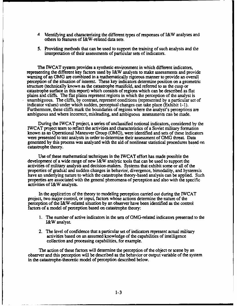
A Tdentifying and characterizing the different types of responses of I&W analyses andothers to features of I&W-related data sets.

5. Providing methods that can be used to support the training of such analysts and theinterpretation of their assessments of particular sets of indicators.

The IWCAT system provides a synthetic environment in which different indicators,representing the different key factors used by I&W analysts to make assessments and providewarning of an 0MG are combined in a mathematically rigorous manner to provide an overallperception of the situation of interest. These key indicators determine position on a geometricstructure (technically known as the catastrophe manifold, and referred to as the cusp orcatastrophe surface in this report) which consists of regions which can be described as flatplains and cliffs. The flat plains represent regions in which the perception of the analyst isunambiguous. The cliffs, by contrast, represent conditions (represented by a particular set ofindicator values) under which sudden, perceptual changes can take place (Exhibit 1-1).Furthermore, these cliffs mark the boundaries of regions where the analyst's perceptions areambiguous and where incorrect, misleading, and ambiguous assessments can be made.

During the IWCAT project, a series of unclassified notional indicators, considered by therWCAT project team to reflect the activities and characteristics of a Soviet military formationknown as an Operational Maneuver Group (OMG), were identified and sets of these indicatorswere presented to test analysts in order to determine their assessment of OMG threat. Datagenerated by this process was analyzed with the aid of nonlinear statistical procedures based oncatastrophe theory.

Use of these mathematical techniques in the IWCAT effort has made possible thedevelopment of a wide range of new I&W analytic tools that can be used to support theactivities of military analysts and decision-makers. Systems that exhibit some or all of theproperties of gradual and sudden changes in behavior, divergence, bimodality, and hysteresishave an underlying nature to which the catastrophe theory-based analysis can be applied. Suchproperties are associated with the general phenomena of perception and also with the specificactivities of I&W analysts.

In the application of the theory to modeling perception carried out during the IWCATproject, two major control, or input, factors whose actions determine the nature of theperception of the I&W-related situation by an observer have been identified as the controlfactors of a model of perception based on catastrophe theory:

1. The number of active indicators in the sets of OMG-related indicators presented to theI&W analyst.

2. The level of confidence that a particular set of indicators represent actual militaryactivities based on an assumed knowledge of the capabilities of intelligencecollection and processing capabilities, for example.

The action of these factors will determine the perception of the object or scene by anobserver and this perception will be described as the behavior or output variable of the systemin the catastrophe-theoretic model of perception described below.

1-3

Exhibit 1-1

Catastrophe Theory-Based M&W Assessment Activities

Estimated EstimatedIOCondiition

Leysir ofAfv

1-4ctr

1.3 OPERAnNAL MANEUVER GROUP CHARACERISTICS

An OMG is a highly mobile military unit which evolved from the Soviet Mobile Group, ahighly mobile tank formation used extensively during World War II and is designed to operatebehind NATO lines. Its mission is to attack or raid valuable targets, destroy or limit the nuclearcapability of the west, disrupt reinforcement supply lines, and maintain a close proximity withNATO troops thereby making the introduction of tactical nuclear weapons difficult. An OMGis designed to facilitate a quick win by destroying NATO defensive capacity and opening asecond front during the offensive.

The introduction of an 0MG appears to be designed to deter the west from deployingtactical nuclear weapons once hostilities start. NATO uses tactical nuclear weapons to partiallyoffset the imbalance of conventional forces that exists between its forces and those of theWarsaw Pact. However, for NATO to use tactical nuclear weapons, Warsaw Pact forces mustbe well separated from NATO forces. If the two forces are in close proximity to each other,there is a risk that friendly forces will be destroyed if tactical nuclear weapons are used.

OMG's do not operate in isolation. They depend upon other military units for support.For the OMG to be most effective, it must arrive behind NATO lines intact. Because of this,an 0MG will attempt to penetrate an opponent's defenses only after they have been weakenedor diverted by first echelon forces. An 0MG completes the breakthrough started by the firstechelon forces. While attempting to break through NATO lines, the OMG will be supported byheavy artillery preparation and a barrage of covering fire. Artillery and air support areconsidered decisive elements in modem combat The two major artillery units supporting theOMG are the Division Artillery Group (DAG) and the Regimental Artillery Group (RAG).Both groups are usually reinforced with nondivisional artillery battalions. Air defense for the0MG is provided by integrated systems of antiaircraft artillery, surface-to-air missiles (SAMs)and interceptor aircraft of frontal aviation. They provide air coverage at all altitudes.

There are several classes of criteria which can be used to identify an OMG. They are thetime at which OMGs will be inserted into battle, the location at which the OMG will beinserted, the activities of other units that will be done in support of the OMG, and the changesthat occur to a military unit prior to its operation as an OMG.

1. Time and Location of OMG Insertion: The places where the OMG is inserted will beweak points in the NATO defense. It is expected that OMGs will be inserted atlocations characterized as having low combat power, lack of defense in depth, andlow force density.

2. Concomitant Activity of Other Military Units: There are a number of activities inwhich Soviet forces will engagt in support of the OMG's penetration of NATOdefensive lines. Among them are the introduction of jammers to disrupt NATO airand fire support nets and command and control in the sector at which the break willoccur, ground based air defense in support of a breakthrough operation; heavyartillery preparation and covering fire barrage immediately before penetration.

3. Changes to Military Units Becoming OMGs: For a military unit to operate as anOMG, it must increase its mobility and self-sufficiency. It will make the followingkinds of attachments: self-propelled artillery; combat engineers; lift capacity; signaltroops to provide long range communication; and increased amounts of fuel andammunitions.

1-5

SECTION 1.4 IWCAT CONCEPT OF OPERATIONS

United States Air Force I&W analysts have the mission of providing a timely recognitionand reporting of changes in military events that are of interest to the United States. Activitiesperformed under the IWCAT contract have reviewed typical I&W activities and have led to theidentification of those classes of problems which are amenable to analytic procedures based oncatastrophe theory. Synectics' IWCAT project staff has determined, in collaboration with the

Soverfment, that the conditions under which an Operational Maneuver Group (0MG) isarmed from an otherwise "normal" pattern of soviet military advance are of sufficient interestto the government to warrant its selection as the appropriate "I&W situation" as specified in theIWCAT statement of work.

The overall concept of operations for the IWCAT project is illustrated in Exhibit 1-2. Theoperation of the IWCAT knowledge development environment involves several major phasesof activity, including the following:

1. The introduction to the knowledgre develo~et environment facilitV provides theuser of the IWCAT facility with a practice use of this facility and a series of "help"and other text files that aid in its use.

2. The generation of 0MG-related test data sets involves a dedicated scenario generatorthat produces groups of indicators whose properties have been chosen to reflect thoseof an OMG.

3. The presentation of test data sets to I&W analysts permits intelligence analysts toundertake 0MG-related threat assessment activities and the construction of an OMGThreat Assessment Data Base.

4. The performance of a statistical analysis of the OMG Threat Assessment Data Base.Creation of this data base as outlined above sets the scene for its analysis with the aidof techniques based on statistical catastrophe theory.

5. The review of the results of this statistical analysis provides a new level of insightinto the processes of perception and threat assessment undertaken by I&W analystsand can set the scene for the development of new types of operational facilities forOMG threat analysis, for example.

1.4.1 MAPPING I&W PROBLEMS TO CATASTROPHE THEORY SURFACES

Catastrophe theory describes a series of structures called catastrophe manifolds whichresemble stylized "landscapes." Positions on such landscapes are specified by coordinateswhose specific values reflect the values of key independent system variables and the corres-ponding values of the dependent variable(s) of the system. The IWCAT project has used thesegeometrical structures to express the relationships between the nature of the intelligence andother information input to I&W analysts (the independent system variables) and their assess-ment (the dependent system variable(s)) of the perceived level of 0MG threat corresponding tothese inputs.

Test data sets corresponding to different values of selected independent variablesassociated with OMGs are presented to selected I&W analysts and others in a knowledgedevelopment activity where these individuals are asked to describe their perceptions of the

1-6

Exhibit 1-2

Overview of the IWCAT Concept of Operations

ITROCUCTION TO THE KNOWLEDGE DEVELOPMENT ENVIRONMENT

A SMPLE OUSE OF THE ENVIRONMENT

GENERATION AND PRESENTATION OF

INDICATOR STATUS DATA TO I&WANALYSTS

INDI~ATOSTA LVE O CFID~E

I SinIed -High-Level

r oM THREAT AESSME NT tNUMBER OF ACTPIE INCATORS LEVEL OF CONFIDENCE

No OMG Threat lIue OMG Warning

I +0MG THREAT ASSESSMENT DATA BASE

7

STATISTICAL ANALYSIS OF OMG THREATASSSESSMENT DATA BASE

Specify Threat Ameasment Data Sub-Set

I Teat for Appropriate Statltical Approach

rConventional Approach or Ca8tatrophe Approach

r REVIEW OP STATISTICAL ANALYTIC RESULTS

1-7

level of OMG threat reflected in these data. The information obtained during this activity isthen analyzed and an attempt made to fit these data to the cusp catastrophe manifold with the aidof a statistical catastrophe theory-based computer program. This process uses methods whichare rigorous extensions of the techniques of linear regression. When the catastrophe manifoldhas been created in this way, it can be used to assess the nature of I&W-related data sets.

There are other factors which influence perception but which are not tractable within thisscheme. These are variously referred to as context variables or tacit knowledge. Thesevariables include general knowledge about the world which influences how judgments aremade. Examples of this kind of knowledge include the time of year at which the judgment hasoccurred and the politico-military context of the problem.

To provide as realistic a problem environment as possible, sets of context variables weredefined and presented to the individuals performing the OMG assessment task as writtenscenarios. These scenarios are called "Treaty Obligation," "Friendly Ally," and "Third PartyHostilities" scenarios. The first of these scenarios would require direct United States militaryinvolvement under particular circumstances; the second places a high level of obligation on theUnited States to provide information to an ally and failure to do this would result in damage toUnited States political and other interests; the third scenario is one in which the United Stateshas no direct interest in the conflict, but monitors it to recognize changes which impact onUnited States interests as they occur.

1.4.2 A CATASTROPHE THEORY-BASED KNOWLEDGE DEVELOPMENTENVIRONMEN T?

A series of activities, described in the IWCAT proposal as knowledge developmentactivities, were undertaken to determine the responses of I&W analysts when faced with thetask of assessing the likelihood that an OMG has been formed, or is in the process of beingformed. Individuals were given a set of data which were designed to resemble as closely aspossible in a study environment the type of data that would be available to an I&W analyst inan operational environment. The data produced during this activity was analyzed with the aidof a nonlinear statistical procedure based on catastrophe theory (developed by Cobb (1978,1980)) in order to investigate conditions under which ambiguous identifications and suddenand gradual changes in I&W assessments can take place.

Analysis of the I&W environment and discussions with the government have led theIWCAT project team to the identification of the following key control factors and behaviorvariables associated with I&W analysis ac ivities.

1. The control factors represent the inputs to the process of I&W analysis. The IWCATproject team selected two control variables (number of active indicators and level ofconfidence) to represent these inputs. The "number of active indicators" variablerepresents the number of indicators which are activated when the analyst makes ajudgment. The "level of confidence" variable represents a measure of the degree towhich a particular set of indicators can be considered to be a true representation ofactual military behavior. Additional information including weather, time of day, andscenario type is also presented to the analyst during the OMG threat assessment task.

2. The behavior variable represents the result of the process of I&W analyst assessment.The IWCAT project team named this variable the analyst's OMG threat assessmentsince this variable represents the perception of the I&W analyst of the likelihood ofthe formation of an OMG from an apparently "normal" pattern of military advance.

1-8

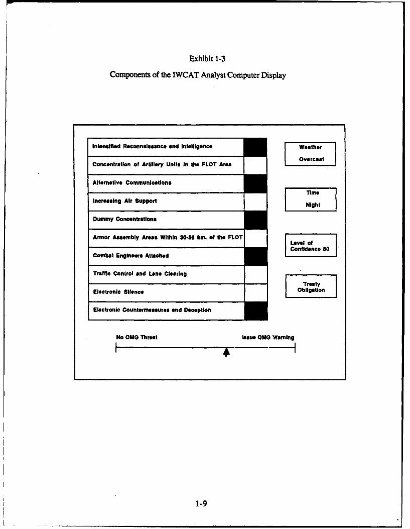
Exhibit 1-3

Components of the IWCAT Analyst Computer Display

Intensified Reconnaissance and Intelligence Weather

OvercastConcentration of Artillery Units In the FLOT Area

Alternative Communications

Increasing Air Support Night

Dummy Concentrations

Armor Assembly Areas Within 30-50 km. of the FLOT iLevel ofConfidence 80

Combat Engineers Attached

Traffic Control and Lane Clearing I Tet

TreatyElectronic Silence ObligaUon

Electronic Countermeasures and Deception

No OMG Threat Issue OMG Warning

I -H-

1-9

The two major control variables described above ("number of active indicators" and"level of confidence") are considered to be independent variables whose values determine thevalue of the dependent or behavior variable, an assumption that can be tested with the aid ofactual analyst assessments and the cusp surface analysis program, as described below. Thus,the number of active indicators and the level of confidence in these indicators provide inform-ation that can permit an I&W analyst to assess the likelihood of the formation of an OMG. Theindependent (number of active indicators and level of confidence) variables can be representedas orthogonal axes and all sets of I&W-related data could be assigned a value with respect tothese axes (see Exhibit 1-1, for example).

In the event that some sets of independent variables create different or ambiguousperceptions of the threat of OMG formation, such behavior could be illustrated with the aid ofthe cusp catastrophe manifold, which is multivalued for some ranges of its control factorvalues. Under these circumstances, some sets of control factor values (the number of activeindicators and level of confidence conditions associated with the I&W-related indicators)generate multiple behavior variable (or 0MG threat perception) values while other sets generatea single behavior variable value.

1.4.2.1 Da Sets

During the OMG threat assessment activities, the I&W analyst is presented with asequence of different data sets each with a different of number of active indicators and level ofconfidence properties which have been chosen to reflect indications of different adversarialstatus conditions that might be presented to I&W analysts during an investigation of whether ornot an OMG was in the process of formation.

Analysis performed by Synectics personnel and a review of several unclassified docu-ments which describe the properties of Operational Maneuver Groups (OMGs) has led to theidentification of the following ten OMG-related indicators (Exhibit 1-3). These indicators arepresented in no particular order to avoid implying any preestablished ranking, importance, orpriority of a particular indicator, or sets of indicators, in the data displays.

1. Intensified reconnaissance and intelligence.

2. Concentration of artillery units in FLOT (Front Line Of Troops) area.

3. Alternative communications.

4. Increasing air support.

5. Dummy concentrations.

6. Armor assembly areas within 30-50 km of the FLOT.

7. Combat engineers attached.

8. Traffic control units and lane clearing.

9. Electronic silence.

10. Electronic countermeasures and deception.

1-10

When using the IWCAT system,the I&W analyst is presented with a level of confidencenumber the value of which reflects the degree to which the particular set of data elements isconsidered to represent an "actual" situation of interest (Exhibit 1-3). In each display, only theindicators listed would be "turned on." The type of scenario (Treaty Obligation, Ally Supportor Third Party Hostilities), and the attendant weather and day/night conditions are alsopresented on the warning display screen.

The analyst forms a judgment as to his or her own relative degree of certainty that thedisplay indicates that an OMG activity is impending, and enters this on a sliding scale at thebottom of the display with the aid of the "arrow" (< and >) keys. The display software thencaptures this registration as a decimal number (0.0 to 1.0), stores it for subsequent statisticalanalysis, and advances to the next situation in the series to be displayed (Exhibit 1-4).

1.4.2.2 The Collection of Test Assessments

In order to determine the reaction of I&W analysts to particular types of data, a selectionof test data sets, each with different numbers of active indicators and level of confidence infor-mation, is presented to the individuals participating in the knowledge development activity.These individuals can undergo an initial period of training and can be asked to review eachelement of the data set for a short time and then provide an assessment of the OMG-relatedposture of an adversary as reflected in these data. This assessment is recorded by indicating aposition on the scale as mentioned above and these assessments are stored in the OMG ThreatAssessment Data Base (Exhibits 1-4 and 1-5).

1.4.2.3 The Processing of OMG Assessment Data

The results for each individual participant are tabulated, recorded, and analyzed with theaid of a statistical catastrophe theory-based computer program (Cobb, 1980) in order todetermine whether the data can be described with the aid of a linear model, or whether the datacould be described more appropriately with the aid of a nonlinear model based on the cuspcatastrophe manifold. Exhibit 1-5 describes the conditions of four different sets of indicatorswith their associated level of confidence values. These four different data sets are consideredto have generated four distinct assessments of the likely formation of an OMG and thisassessment is assumed to have been recorded in the OMG Threat Assessment Data Base andstatistically analyzed (Exhibits 1-5 and 1-6). The number of active indicators and level ofconfidence parameters can form the axes of the control space associated with the statisticalcatastrophe model (Exhibit 1-6).

1-11

Exhibit 1-4

Analyst OMG Threat Assessment and Data Base Formation Activities

SdedOpllon-l Eftwopdon1. Reed ...2. Enter ...3. Make ...

Erder 15Dda 4. Practice ...

15. Take ...6. Make ...7. Perform ...

OtAt...

Start of SeWence

Treaty ObIgation

I Md--

Erftr

End of SeWence

Treaty ObUgAonF- I I I

Enter

Slart of Swpwm

FrIendy Afly Enter Opdon

End of Dda I . Read ...

SKPJWVO 2. Enter ...3. Make ...4. Practice ...5. Take...6. Make ...7. Perform ...S. QA...

1-12

Exhibit 1-5

Relationship of the 0MG Thret Assessment Data Base to theCusp Catastrophe Manifold Control Plane

PFIR820TATMO OF NObOATOM SATUSMI LOWE OF CWWICC DATA

VIOICATOR STATU

c~mnu -- f of ANINy Ulht In o PLOT Ar

A~noCwoewora

uasc Caaom 0m

TMG Ca Owar " XB

STAISTCA ANL I IOd

OW INEATID DATA

amG 0OOMONASM MU

1-13

Exhibit 1-6

Fitting 0MG Threat Assessment Data Base to the Cusp Manifold Surface

Ca~

1-1

1.5 CUSP SURFACE ANAL fSIS

The analysis of the OMG Threat Assessment Data Base in the IWCAT system isperformed with the aid of a program based on statistical catastrophe theory. A catastrophemanifold or "cusp surface" is a statistical model derived from catastrophe theory with onedependent variable and an arbitrary number of independent variables. The cusp catastrophemodel is a response surface that contains a smooth pleat in which the original control variablesand the original behavioral variable have been transformed by a mathematical process whichadjusts the coordinate system so that the shape of the original response surface matches that ofthe cusp surface near the cusp catastrophe point, which serves as the origin of the pleat.

Thus. the canonical behavior variable for the cusp surface model is a function of both theoriginal behavior variable and the original control variables, while the canonical controlvariables (a) and (b) are each functions of all of the original control variables. This is theprincipal difference between the statistical model and the topological model.

1.5.1 ESTIMATING PARAMETERS

The cusp surface analysis procedures of the IWCAT computer system use the method ofmaximum likelihood to estimate the parameters of the cusp model. The conditional probabilitydensity function (PDF) for the behavioral variable (which Woodcock has also called theproperty distribution function) has either one mode or two modes separated by an antimode.Therefore the predictions made by the cusp model are the modal values of the conditionalprobability density function. The antimode is an "antipredicion" - a value that is specificallyidentified as that which is "not likely to be seen."

The differences and similarities between linear regression and cusp surface analysis areworth careful examination. The conditional PDF of a function in linear regression is a normalor Gaussian shaped curve generated from a function that is the exponential of a quadratic. Bycontrast, the conditional PDF of the function of cusp surface analysis is a bimodal curve and isgenerated from a function that is the exponential of a quartic. The predicted values in linearregression are the means of the conditional densities, which also happen to be modes, while incusp surface analysis, the predicted values are modes and the densities are frequently bimodal,yielding two, ambiguous, predictions of system behavior. Lastly, in linear regression theformulas for the sampling variance of the estimators are known exactly, while in cusp surfaceanalysis the corresponding formulas are approximations.

The cusp surface analysis program begins with the estimated coefficients of the linearregression model, and iterates towards the parameter vector that maximizes the likelihood of thecusp model given the observed data. The iterative scheme is a modified Newton-Raphsonmethod. If the very first iteration yields a decrease in the likelihood function, the programimmediately halts with a message indicating that the linear model is preferable to any cuspmodel (this is not a rare occurrence).

1.5.2 MAKING PREDICTIONS

The parameter estimates reported by the cusp surface analysis program are useful forgenerating predictions, but their values indicate nothing about their statistical significance.Therefore the program also reports an approximate t-statistic for each coefficient, with a given

1-15

number of degrees of freedom. These can be interpreted in the usual fashion: magnitudes inexcess of the critical value indicate that the coefficient is significantly different from zero at thespecified significance level, however, these t-statistics are only approximate. Of course, thesestatistics can also be misinterpreted in the usual ways. For example, it is a mistake to payattention to any of these values unless the overall model has passed all of its tests foracceptability.

There is no single definitive statistical test for the acceptability of a catastrophe model.Part of the difficulty stems from the fact that a catastrophe model generally offers more thanone predicted value for a behavior, or dependent, variable given a set of control, or indepen-dent, variables. This makes it difficult to find a tractable definition for prediction error, withoutwhich all goodness-of-fit measure that are based on the concept of prediction error (e.g., meansquared error) are nearly useless. Another part of the difficulty arises from the fact that thestatistical model is not linear in its parameters. And finally, of course, it is scientificallyunsound to base any definitive statement on the analysis of a single data set, no matter what itsstatistics show. Confirmation must always be sought in the independent replication of results.In spite of these difficulties and caveats however, there are a variety of ways in which acatastrophe model may be tested through statistical means.

Cusp surface analysis offers three separate tests to assist the user in evaluating the overallacceptability of the cusp catastrophe model (Exhibits 1-7, 1-8, and 1-9). The first test is basedon a comparison of the likelihood of the cusp model with the likelihood of the linear model.The test statistic is an "asymptotic chi-square," which means that as the sample size increasesthe distribution of the test statistic converges to the chi-square distribution. The degrees offreedom for this chi-square statistic is the difference in the degrees of freedom for the twomodels being compared. Sufficiently large values of this statistic indicate that the cusp modelhas a significantly greater likelihood of being "correct" than has the linear model.

The cusp catastrophe model may be said to describe the relationship between a dependentvariable and vector of independent variables if all of these three conditions hold:

1. The chi-square test shows that the likelihood of the cusp model is significantly higherthan that of the linear model.

2. The coefficient for the cubic term and at least one of the coefficients of the factors Aand B are significantly different from zero.

3. At least 10% of the data points in the estimated model fall in the bimodal zone.

In the literature on applications of catastrophe theory there are two distinct ways ofcalculating predicted values from a catastrophe model. In the Maxwell Convention thepredicted value is the most likely value, i.e., the position of the highest mode of the probabilitydensity function. In the Delay Convention a mode is also the predicted value, but the modeoccupied by the system is not necessarily the highest-valued mode. Instead, the predictedvalue is the mode that is located on the same side of the antimode as the observed value of thestate variable. Thus the delay convention uses as its predicted value the equilibrium pointtowards which the equivalent dynamical system would have "moved." The delay conventionis most commonly adopted in applications of catastrophe theory, but there are circumstances inwhich the Maxwell convention is more appropriate.

1-16

Exhibit 1-7

A Conventional or a Catastrophe Theory-Based Approach?

OMG THREAT ASSESSMENT

NUMBER OF ACTIVE INDICATORS ILEVELOF CONFIDENCE

No OMG Threat Issue OMG WarningI I

OMG THREAT ASSESSMENT DATA BASE

STATISTICL ANALY

SPECIFY ASSESSMENT

DATA SUB-SET

• Specify Number of Variables

• Specify Positions of SelectedIndependent Variables

* Specify Position of SelectedDependent Variable

DPLAY RESULTS

USE STATISTICAL CATASTROPHE THEORY APPROACH

1-17

Exhibit 1-8

Criteria for Acceptance of the Cusp Catastrophe-Based Model

CUSP SURFACE ANALYSIS

TESTS FOR EVALUATING ACCEPTABILITYOF CUSP CATASTROPHE MODEL

ASYMPTOTIC CHI-SQUARE TEST

To determine whether the likelihood thata statistical cusp model is a better fit for

the data than a linear model

CUBIC TERM ANALYSIS

To determine If the coefficients for the cubicterm and at least one of the other coefficients

are significantly different from zero

DATA LOCATION REVIEW

~To determine If at least 10 percent of thedata points of the estimated model are

located In the bimodal zone

IF CRITERIA ARE SATISFIED

USE STATISTICAL CATASTROPHE THEORY APROC

1-18

Exhibit 1-9

Cusp Surface Analysis: Making Predictions

CUSP SURFACE ANALYSIS: MakingPrdcin

Maxwell Convention: Delay Convention:

Predicted value is the most likely value, Predicted value is the mode that is locatedthat is, the position of the highest mode on the same side of the antimods as the

of the probability density function observed value of the state variable


Calculates the predictions made under the Maxwell andDelay conventions for each datum and derives statisticsand graphs to evaluate the quality of their predictions

Mo nd Antimodas

DsR S t s t ic

lMxwel-R Statistic

Error Histogram

1-19

1.6 0MG THREAT ASSESSMENT ANALYSES

The IWCAT system software was used in a series of tests during which individuals withexperience in the indications and warning and intelligence analysis areas were asked to assessthe perceived level of Operational Maneuver Group (OMG) threat associated with a series ofsets of 0MG-related indicators (Exhibit 1-10). The IWCAT system permits the creation of anOMG threat assessment data base and its subsequent analysis with a nonlinear statisticalprogram based on statistical catastrophe theory in order to construct a mathematical model ofthe data which could be used as the basis for further analysis of the responses of I&W analyststo situations of interest.

When a nonlinear model can be constructed from the analysts threat assessment data, it ispossible to describe a range of different I&W analyst response behaviors such as sudden andgradual perceptual changes, divergence, ambiguity, hysteresis, perceptual "trapping," andcounter-intuitive or paradoxical behavior. One particularly interesting discovery providesstatistical evidence which suggests that I&W analysts with different types of training andprevious mission responsibilities appear to respond to different features of the OMG threatassessment data set.

1.6.1 MAPPING DATA TO THE CATASTROPHE MODEL SURFACE

The IWCAT system uses the method of maximum likelihood to estimate the parametersof a model based on the observed data and, when a cusp-based model can be constructed,performs statistical tests to determine whether a linear or the cusp-based model provide a betterdescription of the data. A cusp-based model of the data is accepted when the chi-square testshows the likelihood of the cusp model to be significantly higher than that of the linear model;the coefficient of the cubic term and one of the other coefficients of the cusp model aresignificantly different from zero; and at least 10% of the data points in the estimated model fallin the bimodal region (see Section 4., for example).

In the process of constructing the cusp model, the system transforms the input data to fita cusp surface. This surface is an inherently three-dimensional object which can be drawn as astructure with three axes, each of which represents a component of the cusp model. Two ofthese axes represent the control factors or input variables and the third axis represents thebehavior or output variable of the system of interest and positions on the surface can be locatedwith respect to the values of these three axes. The two control factors, which may themselvesbe a function of other variables, define a plane called the control plane.

The 1WCAT system provides the user with a series of diagrams which display thefeatures of the cusp model. In one display (see Exhibit 1-11, for example), the transformeddata are presented as locations on the control plane formed from (transformed) versions of thecontrol factors called the bifurcation (or splitting) and asymmetry (or normal) factors. Basedon this analysis, it is possible to construct a cusp catastrophe model that is the best available"fit" for the I&W analyst-derived data (see Exhibit 1-12, for example). The (transformed)actual data is located within the circle drawn on the control plane formed from transformationsof the number of active indicators and level of confidence control factors. In this particularcase, some of these data lie inside, and the remainder lie outside the region of bimodality orambiguity on the control plane. A linear model of the data is highly appropriate when all thedata points lie outside the region of ambiguity.

1-20

Exhibit 1-10

IWCAT System Activities

TEST DATA FILE CONSTRUCTION

" Active I&W Indicators" Level of Confidence" Scenario Type" Weather* Time of Day


• I&W Analyst Assessment" OMG Threat Data Base

STATISTICAL ANALYSIS OF OMG THREATASSESSMENT DATA BASE

* Specify Data File to be Analyzed* Identify Sub-set of Indicators for Analysis" Test for Appropriate Statistical Approach" Compile Statistics from Analytic Procedures" Review Results of Statistical Analyses

CUSP CATASTROPHE-BASED MODEL

* Mapping Data to the Catastrophe Model Surface* "Slicing" the Cusp Manifold" Sudden and Gradual Perceptual Changes• Divergence" Ambiguity" Hysteresis" Perceptual "Trapping"• Counter-intuitive or Paradoxical Behavior

" Identification of Analyst-Specific Responses* Implications for On-going I&W Activities

1-21

Exhibit 1-11

I&W Analyst-Deived Data Plotted on the Control Plane of the Cusp Model

Location of data in the control spacer

Vertical axis: Rifureatin (splitting) factorHorizontal axis: Asymmetry (normal) factorAsterisks& Bimodal zone

-5 -4 -3 - -1 0 3 a 3 4 5

5.0 000000000000000000000 5.0

4.5 000000000000000000000 4.5

4.0 000000000000000000000 4.0

3.5 000000000000000000000 3.5

3.0 000000030000000000000 3.0

2.5 0 0 0 0 0 0 0 4 4 2 0 0 0 0 0 0 0 0 0 0 0 2.5

2.0 00 00 0 00 7 a 08 is 00 00 00 0 00 2.0

1.5 0000000000 9000 000000 0 1.5

1.0 0 00 00 00 0 00 7 10 90 0 00 00 0 00 1.0

0.5 0 0 0 0 0 0 0 0 0 0 0 0 & 0 0 0 0 0 0 0 0 0.

0.0 0 0 0 0 0 0 0 0 0 0 0 0 0 0 0 0 0 0 0 0 0 0.0

-0.5 0 0 0 0 0 0 0 0 0 0 0 0 0 0 0 0 0 0 0 0 0 -0.5

-1.0 00 00 00 00 00 00 00 00 00 0 00 -1.0

-1.5 0 0 0 0 0 0 0 0 0 -0 0 0 0 0 0 0 0 0 0 0 0 -1.5

-2.0 0 0 0 0 0 0 0 0 0 0 0 0 0 0 0 0 0 0 0 0 0 -2.0

-1.5 00000000 0000 000000000 -1.5

13.0 00000000000 03000000000 -1.0

03.5 000000000000 00000000 03.5

-4.0 0 0 0 0 0 0 00 0 0 0 0 0 0 0 0 0 0 0 00 04.0

-0.5 000000000000000000000 -0.5

-1.0 000000000000000000000 -1.0

-2.5 0 0 0 0 0 0 0 0 0 0 0 0 0 0 0 0 0 0 0 0 0 -3.5

0 c0ses did 00t fit 0n the above 0igure.

Linear R 0 0 0 0.0 (0 0lti0le r0r0ss.on)D 5y R^ - --.472 (0tt1acti -2de convention)

Maxwell R^2 - -0.219 (Most-likely-mode convention)

SNegative R-8 values occur wen the cusp model is worse than a constant.

>) >> Fraction of case* in bimodal zones 0.415 <<<<

1-22

Exhibit 1-12

Mapping Data to the Cusp Model Surface

Model o Number of ActiveSurac wfnd.wIndicator

L nalel oode ofnrCo sesmentan

of OMGAc1-23

1. Sudden and Gradual Perceptual Changes. The cusp model constructed from I&Wanalyst-derived data describes conditions under which sudden and gradual changes inanalyst perceptions can take place (see Exhibit 1-13, for example).

2. Djiygnc. The cusp model can also illustrate the property of perceptual divergence,as shown in Exhibit 1-14) where relatively small differences in the initial level of de-tail can have a profound impact on the nature of the analysts OMG threat assessment.

3. Ambigily. Preconditioning can lead to perceptual ambiguity, a phenomena which isillustrated with the aid of the cusp surface model shown in Exhibit 1-15.

4. "Slicing" the Cusp Surface. The IWCAT system provides the user with a series ofdiagrams representing "slices" of the cusp model surface in which all but one of thecontrol factors are held fixed at their mean values and the effect of changes in theremaining factor on the shape of the surface is displayed (see Exhibits 1-1 6a and1-16b, for example).

5. Pe tual Hysteresis. The phenomena of "perceptual hysteresis," may be illustratedwith the aid of the cusp surface model (Exhibit 1-17).

6. Ercptual'raijng." Use of the IWCAT system by a series of analysts has led tothe characterization of a phenomenon which Woodcock has called "perceptualtrapping." Exhibit 1-18 illustrates the phenomena of partial perceptual trapping whileExhibit 1-19 illustrates complete perceptual trapping.

7. Counter-Intuitive or Paradoxical Behavior. Cusp surface models based on analyst'sperceptions of OMG threat suggest that the analyst's perceptions may exhibit patternsof counter-intuitive or paradoxical behavior, as shown in Exhibit 1-20.

1.6.2 SPECIFIC ANALYST ASSESSMENTS

As mentioned above, several members of Synectics staff who have been involved invarious forms of I&W and intelligence analysis activity participated in testing the IWCATsystem. The following constitutes a summary discussion of the results of these different testsand a detailed analysis of these results can serve as a starting point for further researchinvestigations and for the development of an operational IWCAT facility.

In each case the analyst was presented with a test data set of indicators and other infor-mation described in Section 5, and asked to assess the level of OMG threat that they appear toreflected to the analyst. Following this task, the analyst was asked to designate which of theindicators were of primary importance and which were of secondary importance in determiningthe level of perceived OMG threat. Information generated by this process was then subjectedto analysis using the cusp analysis program.

It is a suggestive finding of this statistical analyses performed during this investigationthat the nature of the response of the different analysts to the OMG threat test data appeared todepend upon their background and experience. Thus analysts with extensive active dutymilitary experience (Analysts B and C below) appeared to pay almost exclusive attention to thenumber of active indicators; another analyst (Analyst D below) with much more national levelintelligence analytic experience appeared to pay almost exclusive attention to the patterns (orsequence type) of the displayed indicators. Analyst A, with extensive military experience

1-24

Exhibit 1-13

Cusp Model of Sudden and Gradual Changes in Analyst Perceptions

AnalLeve of Nube nube Acativeidiatr

kawOMG aneiThreat thea

Hig &xdeninceae i t1-25~e

Exhibit 1- 14

Cusp Model of Divergent Perceptions

ondniLevel ~ vrec of Number IniaosfActive

Warning ~Small diffenc a)in perceivedtra

Analyst TIIhoAssessment

of OMVG iLarge difference (b-d)pecie

Threat LO npecie threat

~NoCMGThreat

1-26

Exhibit 1- 15

Cusp Model Can Provide a New Understanding of the Causes of Perceptual Ambiguity

Level of JNumber ofActive

ColtlneIndicators

~Ambiguity in perceptioncas by "pre-conditioning'

Threatreat

//l- Number of Active IndicatorsLevel ofj[ l

~Region of Ambiguity

1-27

Exhibit 1-16

"Slicing" the Cusp Surface

Leve Of Number of Active

TThreat

(a). Fixed Number of Active Indicaors and Variable Level of Confidence Level of Confidence

CofdneNumber t Active Idctr

(b).Fixd Lvelof onfienc wi Vw~ieNumber of Active Indicators

1-28

Exhibit 1-17

Perceptual Hysteresis

4 Decreasing number ofactive indicators

ThreatSudden increasein percived OMGThreat Level

Sud~den decrease

Increasing number ofactive indicators

Range of available Number of Active Indicators

Level of Confidence Variable fixed at its mean value

1-29

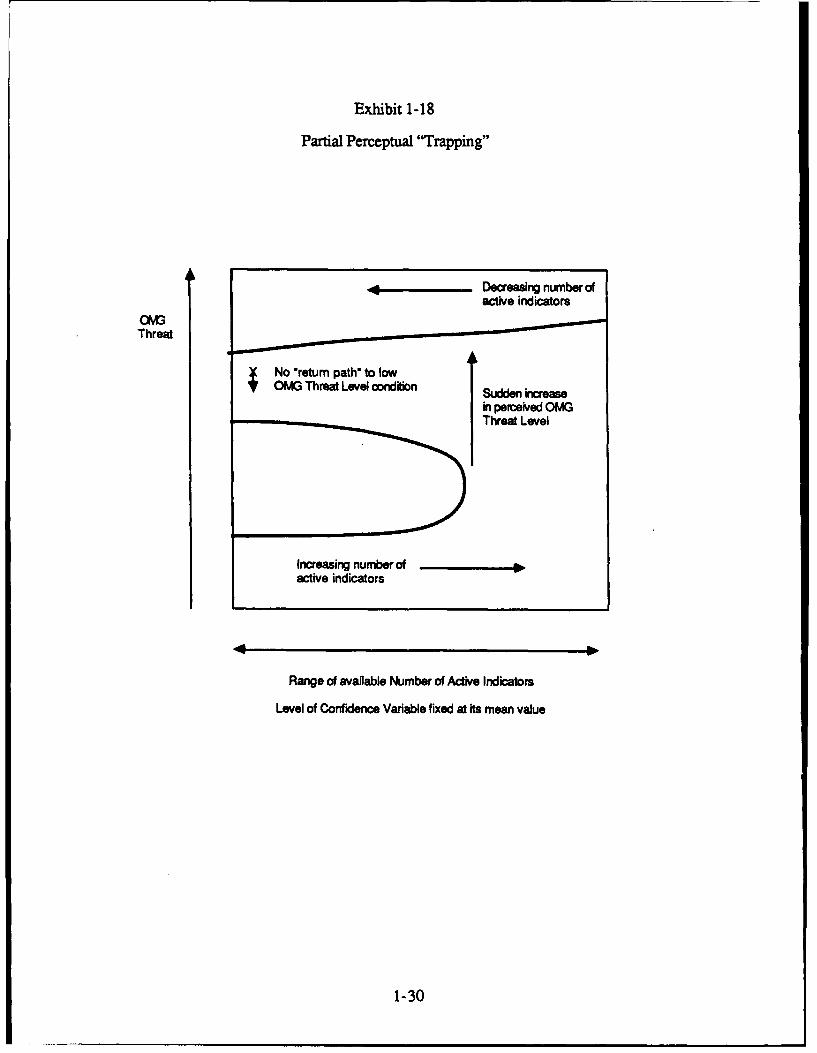
Exhibit 1-18

Partial Perceptual "Trapping"

In ~ ~ ~Dcreasing number of______acttive indicators

Levhel t fniene Vardiabixed tiSudmen vnalue

1-3

Exhibit 1-19COxP~et Pexveptaj -rrappig"

Threat Osavain Nubmber

of Active Ifldicatom

No return Path- to lowV Ot . threat level cndiaon.

No *retr, Path- to high0MG threat level codhio

Range of availabl~e Number of Active Indicators,Level of confidence Varae~ fixed at ftq Mean value

1-31

Exhibit 1-20

Counter-Intuitive or Paradoxical Behavior

Increasing number of

active indicators

ThreatSudden and paradoxical decrease in level ofperceived OMG Threat caused by an increasein the number of active indicators presentedto the analyst

Increasing or decreasing the number of active indicators causesno sudden change in level of perceived OMG Threat while movement

takes place on the lower" part of the catastrophe surface

Number of Active Indicators

Level of Confidence fixed at its mean value

1-32

and involvement in more national level intelligence analytic activity appeared to pay attention toboth number of active indicators and their pattern. Analyst E, with national level weapons tar-geting experience, performed the test. However, the data collected in this process appeared toform a linear model since the cusp analysis program terminated its activities because no cubicterm was detected.

While the observation that the nature of analyst perceptions of OMG threat is predicatedby the nature of the experience and training of the analysts, is a tentative finding due to thesmall sample size of analysts that were used in the experiment, such a suggestion can haveprofound implications on the way that I&W and other forms of intelligence analyses areperformed. Results of the IWCAT project suggest that analysts (who could be referred to as"front-line" analysts) closely associated with the more immediate or tactical aspects of thecombat environment concentrate on the number of active indicators while those analysts (whocould be referred to as "headquarters" analysts) who are involved in the analysis of the morestrategic aspects of combat, and who may receive most of their intelligence input from thefront-line analysts, appear to pay more attention to detecting a pattern in the indicator series.

If substantiated by further work and analysis, such a finding can have an importantimpact on the relationships between these front-line and headquarters analysts since the firsttype of analyst acts as a perceptual filter for the information that is presented to the second typeof analyst. The fact that these different types of analysts concentrate on different aspects of theavailable intelligence information (such as the number of active indicators or the pattern ofindicators, for example) could introduce unexpected and unintentional biases in the inter-pretation of this information and lead to a misunderstanding of the nature of particular combatsituations. The possibilities of such perceptual disconnects and their impact on I&W andcommand and control (C) should be of concern to I&W analysts and others and furtherinvestigations of this suggestion with the IWCAT system would appear to be appropriate.

1.6.2.1 The Perceptions of "Analyst A"

The following is a brief review of the analysis of the I&W OMG threat data collectedfrom one of the five analysts (designated here as "Analyst A"), who are members of Synecticsstaff and who have all had experience as intelligence analysts. More detailed informationconcerning the results of this analysis are presented in Section 6.

1. Impact of the number of active rimary indicators and level of confidence on OMGthreat pction. Exhibit 1-21 presents the analysis of the effect of the number ofactive primary indicators and level of confidence on OMG threat perception. Thecontrol plane plot (Exhibit 1-21 a) shows that 51.1% of the data are located within thebimodal zone and represent analyst assessment conditions which are subject toambiguity. Slices of the catastrophe model surface for a range of numbers of activeprimary indicators and with the level of confidence fixed at its mean value revealsituations in which partial perceptual trapping can occur (Exhibit 1-21b). Slices ofthis surface for a range of values of the level of confidence variable and with thenumber of active primary indicators fixed at their mean value reveals situations inwhich perceptual hysteresis can occur (Exhibit 1-21c) as the level of confidence isincreased or decreased.

2. Impact of the number of active secondary indicators and level of confidence on OMGthreat R r ion. Exhibit 1-22 presents the analysis of the effect of number ofsecondary indicators and level of confidence on OMG threat perception. The control

1-33

Exhibit 1-21

Analysis of 0MG Threat Assessment Data

0) Car"~ PWMs P1W

a.00t 00 iot *9 0 03 a 0 0 0 00oo0

6e.0.. 0 0s 081.o~t. o 95 o tsq 0 09ooo58 0*0 .

-. -A .3 - 0 9

.5 00 0 0 0 0 0 0 0 0 0 0 0 0 0 0 0 0 0 0 0 *.g

0.0 *0 00 0 00 0 1 .a0aIa0 00a0 0 0 2.0

11.11 0 0 00000a0 003I.so0 00 00 00 0 R.5

3.0 0 0 00 0 00093380 0 00 00 0 0 1.0

0.5 0 0 0 0 0 0AS 2I30 0 0 0 0 0 0 0 05.0.0 0 a0 0 0 0 00 00 0 00000 0 .0

0.11 0 0 0 0 0 a 0 0 0 0 0 0 0 0 0 0 0 0 0 0 0 8*.5

8S.0 0 0 00 0 aa0 0 0 00a0 0 0 000 a3-.0

01.5 00 00 00 00 0 00 00 00 00 0 00 00-.1

-4201-6 00 00 *00 00 0 0 0 -0.o,

-. 0 00 0 00 0000 0 000 0 00 0 00 00 -3.0

-. 11 0 0 0 0 0 0 0 0 6 0 0 0 0 0 0 0 0 0 0 0 0 -8.5

-. 0 0 0 0 0 0 0 0 0 0 0 0 0 0 0 0 0 0 0 0 0 0 -. 0

LA 0 P-11 :16 -pst01 -r - 13 0 3

O08., 00 * 0.311 Mqltt.eq-0 e..t095.8 0*0.110 9 5.8t8~.O~*

)fl)) VottsS S a, ,95.8 ala6.1113 "".48

000..8 qf e8950 0. 30.o.ft &IS S~*M. at Ift0 ed- "18a. £090 e.580.05a al*06 3040 Ut . 8

-a 4 B 0 3 0 5 - 0 -s 0 3 3

0.0 . C 0.0 0.0 I* 0.

8. 0 0.:87 0.

3.0 0 * 8.0 80 * .3.5 ~ a do C 0 85 .30 .

3.0* 0 0 8.0 3.0 9 C 3..8.5a T I -.5 3. *C

8.0 * 0 C 3.0 .0 .

8.8oar * ~w Lee of 8.8er 3. 8.

lo.0 .. " *f 8. 80 " 8.0.9 Mos * WM. AMSMN * .9 0. 0C .

1b) *albernuy 0mL*jc~M 0) 0.0ew Leve of 0okere 0bo 0.0wy

0.7 * . 0. 0.7 0-0.

Exhibit 1-22


(a) Cor*oi PIw Plot

&M f do" A. C 9.i .I

".-"I 830... C.3 4w 3C1q 1 .

41 g 0 4 - -0 0 0 0 * 0 UC.0 *OOOOOCOCCCOCC@00 0 0 00 4.0

O.1 *eeeo@C o eaQaa0 00eee. a S.C0

6.1 * 0 0 0 S 0 S S * n so o 0 0 C ** i

-S.6 0 0 0 6 0 0 6 0 41 0 *3C 0 0 0 0 0 0 a S 0.0

*~ * OOSO ee~e SO~e S~ge .4.0

-3.* 00 0 0 0 0 S 0 0 a 0 a 0 0 -0.0

-. U0 0 0 0 0 0 0 0 0O 0 0 ** 0 0 0 0 -3.

05. 0 0 0 05 0S 0 0 0 0 0 0 0a 0 0 -4.0

LA- 0 *.Sh, filole C35

pppo . - S8.34ShS .. ,.oq- ~O. CC4

9#110 .-d~l.a.m~~f .1 ,f- S, k 0- "SOS emIM me-a n, S-Abs1eMig9 2 ~%M.,

C., Tho 1.0.1 Tm

*4d CC CmC.

* . *

0.

5.3~~~Z la e,*

.4.. C 0 * .0 -4.0 ...0:.1 . C-.5. .0 : .4.1.4, oo 5m* .eAm .01, 31 .4.,f agam

-3.5 .0 0 .1-5. .3 C-I

plane plot (Exhibit 1-22a) shows that 53.3% of the data are located within thebimodal zone and represent analyst assessment conditions which are subject toambiguity. A slice of the cusp surface at a fixed level of confidence and variablenumber of active secondary indicators reveals situations in which perceptual trappingcan occur. Increasing the number of these active indicators from a low to a higherlevel causes a gradual increase in perceived OMG threat to a condition at which asudden change in these levels can take place (Exhibit 1-22b). A slice of the cuspmodel surface for a range of values of the level of confidence and with the number ofactive secondary indicators fixed at their mean value reveal situations in whichperceptual hysteresis can occur (Exhibit 1-22c) as the level of confidence is increasedor decreased.

3. Impact of number of combined active primary and secondary indicators and level ofconfidence on OMG threat2cetion. Exhibit 1-23 presents the analysis of the effectof the activity number of all indicators and level of confidence on OMG threatperception. The control plane plot (Exhibit 1-23a) shows that none of the data arelocated within the bimodal zone. This finding is also confirmed by the data presentedin Exhibits 1-23b and 1-23c. The comparison of the material presented in Exhibits1-21, 1-22 and 1-23 is revealing. While analysis of the data set in which the primaryor secondary active indicators provides graphs which suggest that sudden changes inperception can take place, analyzing the effect of these indicators as a whole reveals alinear response characteristic. Under such circumstances, the combination of theresponses generated by the simultaneous consideration of the effect all the indicatorscan be described with the aid of a simple linear model. This demonstrates a majordifficulty that might arise when data of different levels of importance to an analyst arecombined for statistical or other purposes. Such observations should be a matter forfurther consideration.

4. Impact of sequence type and level of confidence on OMG threat perception. Exhibit1-24 presents the analysis of the effect of sequence type and level of confidence onOMG threat perception. The control plane plot (Exhibit 1-24a) shows that 41.5% ofthe data are located within the bimodal zone and represent analyst assessmentconditions which are subject to ambiguity. A slice of the cusp surface at a fixed levelof confidence and variable sequence type reveals situations in which perceptualtrapping can occur with the analyst's OMG threat perceptions restricted either to ahigh value range or a low value range (Exhibit 1-24b). A slice of the cusp modelsurface for a range of values of the level of confidence and with the sequence typefixed at their mean value reveal situations in which perceptual hysteresis can occur(Exhibit 1-24c) as the level of confidence is increased or decreased.

5. Impact of number of active _nmamry indicators, sequence type, and level of confidenceon OMG threat Verception. Exhibit 1-25 presents the analysis of the effect of numberof active primary indicators, sequence type, and level of confidence on OMG threatperception. The control plane plot (Exhibit 1-25a) shows that 54.8% of the data arelocated within the bimodal zone and represent analyst assessment conditions whichare subject to ambiguity. A slice of the cusp model surface for a range of values ofnumber of active primary indicators and with the sequence type and level ofconfidence variables fixed at their mean values reveals situations in which partialperceptual trapping can occur (Exhibit 1-25b). A slice of the cusp surface at a fixedlevel of confidence and number of active primary indicators and variable sequencetype reveals situations in which perceptual trapping can occur with the analyst's OMGthreat perceptions restricted either to a high value range or a low value range for allranges of sequence type values (Exhibit 1-25c). A slice of the cusp model surface fora range of values of the level of confidence and with the numbers of active primary

1-36

Exhibit 1-23


(a) Coimol P1., Plot

89.0 0 0 a 0 4 0 0 0 060*000 .

.9 0 808 0 0 0 6 a8899' 0 a0mw 00 .

3.110 * 0 s

-. . -. .4 .4 0 00a 0 * 0 1 0 1

1.~~ ~0 0 0 4 0 0 0 0 00 0.

0. e0 0 00 00 000000 0.0

a. *0 0 0 0 0 0000 0.

1. *. 0 . . o o . . . o a .,

-0., 0 0 0 0 0 * 0 0 0 0 0 0 0 0 0 0 0 0 0 0 0 -0.9

-8.0 *00 0 *0 0 0 0 0'A00 0 0aS0 00 0 I.S

08.0 *.Se a0 0 00 9130 0060 00 *0 00 -0.0

0.11 0 000 &0 00 0 00 00 000 0 000 * 0.5

-8.0 0 0 0 60 *a0 0 800 a0 0 **00 0 0 -2.0

-2.1 0 0 0 0 a0a 0 0 a 0 0 0 0 0 0 0 0 0 41 * 0 -. 2

.0 0 0 0 0 0 0 0 0 3 0 0 0 0 0 0 0 0 0 0 .4.

.% a 0 0 0 0 0 0 0 0 0 0 a 0 0 0 0 6 0 .5

-. 1 0 0 0 0 0 0 0 0 0 0 0 0 0 S 0 0 0 0 0 0 S -. 0

* Sa itte fi 09 30 0- 10-0.

PiNS l Wiii 0..00 ...8908 44.5

aft- .. . f. 41ise '&I O0. istta.. 0 ~. immt a. Offat of 1.4.0. ft.83. .11 _."att .4 N a' itti. t

1 ~ ~ ~ ~ ~ ~ :8 to- l 4 .

0.1* 0 :51 0 0.

0.3 * ~0.8 .9..0 * . 00* .

.9* * .9 8. * 8.A.I0 - I . . .

(b)* *WW A.N 8.7mlm Fie U"o8., C ~rb rWo atrm ie IW

3.4* 8.0 8.0 1-37.

Exhibit 1-24


or iNd A.lo atil'e qp

"I*.a 00 0 41-fO S.0 *,11011.19 9-ft,

Gdod'ta.. oidiNNI -

-g - 0e GO - * 0 0 * 0 5

a.0 * 00 0@0 00 000.0a0 0 00 03.

0. 0 a 0 OO 0 A, aa O 0 a 0 00 5.0

0. *06 a00 0 0 000 S 00 0.0

. 0 0000 a00 0 0 000 .

53 0 0 0 0 0 0 * IN a 0 to e 5 0 0 0 0 0 0 0 0 5.0

.0 0 0 * 0 0 0 0 0 0 0 750 .

0. 0 o 0 00 0 0 0 00 .

. 0 0 d.0a0000 0 0 300 3.0Q s

-0.5 o*0a0 0 0 0 00006. -0.-5.0 0 0 a 0 0 0 00 0 0 0 : 0 000 -.

-0.0 S 0 0 0 0 0 0 a 9 0 0 0 0 0 0 0 0 0 a a 0 [email protected]

-0.0 0 0 a0 0*0 a*0 * 0 000 0 0 00 00..0

.S 0 0 0 0 0 0 0 0 0 0 0 0 0 0 0 0 * 0 0 a .110

.01 0 0 0 0 0 0 0 0 0 50 0 0 0 0 a 0 0 .o

-90 0 - 3 0 0 05 0 5 3 0 0 3 -.

0di d id -IL fisaft da- fsq

Lin 78 gote st, 1.6 .- I~f.t

-I-.di rs 0. si..n diddit e . n .

*5)5 ft.S. of - l .. na n . 0.455 944444

-. ~~~~--- --- *3 3.35 0

0.0 .. 0.5 0.5 .. 0.

0..ive . 00 01 * 0

0.9 . ~010. . .

0.0 *. 0 400.0 :

i KPe. TYP :. L" d~~qg * sod5.700 ., 1 5.7

lb w...w=T".Fa fl.,gg d Cod .c Vmft OMWg of.7boFa ww

5.5* 0 5.0 5 I1-38.

Exhibit 1-25

Axiysis of 0MG Thret Assessment Data

(a) Con~v Pamm Plot

0*to 0 it 90 0 a a 0 a0000000000 C

00... *...1 0 0 0a00a000 .

-. 0 -3 -. 0 a 0 5. 0 0

0 *0 0 0 0 S00S001070 0 0a0 0 .

0. 0o~ o o 0a l 00000008 93%-0 8.0

3.1 600 0 0 0 0 00 0000* .

0.20 0 0 00 0 0 00 0 000000 0

0 01 00000 10 100 0 0 0 000 -0.1

08.0 0 0 060 00 0 a 0300000. .

0 0 000*0 00 0 000 00 00 00 00 0 0

-0.2 *00*0 0 00 00 000 060 00 0 000 .0.3

-2.0 0 a a 0 0 0 0 0 0 0 0 0 0 0 0 0 0 0 0 0 0 -8.0

-5.0 0 0 0 0 0 0 0 0 0 0 0 0 0 0 a a 0 0 0 0 0 -. 0

-. S 0 0 0 a 0 0 0 0 0 0 0 0 0 0 0 0 0 0 0 0 0 .S

4S.0 0 0 0 0 * a 0 0 0 a 0 0 0 0 00 0 0 0 0 0 -S.0

0 - . -1 -IS 9. -. .0 a140-0

0 o. ,000 fat . to .0

l..ll 00* 0.1 * a 1 0 r 0 .0 0.,,

* 0.9 0.

-. 0 30Psr~~ved :------.--------a dfw ww" * .7 a.. MTflug

a., a..tPmr'I- FbdsqneTp c)V~ euwTp, be ~.m clL"0 o.. .~dw a..UWofCik

.1 . . * a.1 1-39.

Exhibit 1-25 (Continued)

Analysis of 0MG Thireat Assessment Data

*.a . 0.85.0~~- 1 . . .

q*mpW Hyrw. * *

T'5 L" d Cafte* s

a.: .,.

8.7* l a.,o knidne ie wir imdr

aid ~ ~ 8.9ev Tp

a.. * 1 a.

indicators and sequence type fixed at their mean values reveals situations in which perceptualhysteresis can occur (Exhibit 1-25d) as the level of confidence is increased or decreased.

1-41

SECTION 2. THE IWCAT EFFORT IN CONTEXT

The Indications and Warning Applications of Catastrophe Theory (IWCAT) effort hasdetermined that it is feasible to use catastrophe theory and related state-of-the-art mathematicaltechniques to provide new facilities to support the activities of I&W analysts in areas ofimportance to the United States Air Force. Investigations have concentrated on the use ofindicators related to the formation of Operational Maneuver Groups (OMGs) as a test of thesystem. This effort has involved the development of a new flexible and adaptable problem-solving and decision-making environment that is able to captr-re and use small, and apparentlyinsignificant, changes in information that are the precursors of dramatic changes in overallsystem behavior.

This final technical report identifies a specific I&W-related problem which is amenable toanalysis with the techniques of catastrophe theory. In general, suitable problems will be thosein which several key influences determine system behavior. I&W problems of interest exhibitsome or all of the following properties:

1. Gradual and sudden changes, divergence, bimodality, and hysteresis that arecharacteristic of the behavior exhibited by the elementary catastrophes.

2. Small changes in the information provided to an analyst can give rise to either smallor large changes in perception under the same conditions.

3. Small biases in information can give rise to dramatically different analyses.

After extensive discussions with the government, the IWCAT team selected an I&Wproblem which involved the recognition of an OMG, one of the most difficult problems intactical analyses. A set of ten indicators predicting the development of a Soviet OMG wasdeveloped. Settings of these indicators were presented to military analysts who were asked toassess the probability of OMG development and the resulting assessments were captured andanalyzed with the aid of a statistical program based on catastrophe theory.

2.1 NEW FACILITIES ARE NEEDED TO SUPPORT THE I&W ANALYST

Military analysts and decision-makers in the Indications and Warning (I&W) area arefaced with the need to analyze and understand large amounts of often conflicting and contra-dictory data derived from sensors, communications systems, and other sources. These tasksoften have to be performed under severe time-pressure and if used in the field, at some actualphysical risk to the analysts and decision-makers themselves. Faced with the problem ofinformation overload in critical periods of combat, such individuals will have to resort to theuse of analytic methods that capture the essence of system behavior and "friendly" graphicsdevices that can facilitate the understanding, reasoning, and decision-making activities ofanalysts in ways that develop and reinforce their perceptions. The IWCAT effort has produceda prototype computer-based system that can support the I&W analyst by providing a newtechnology for capturing I&W analysts' perceptions of situations of interest and communi-cating their understanding to battlefield commanders. The IWCAT technology can also be ofvalue of I&W analysts and decision-makers by:

1. Alerting individuals to conditions where small changes in indicator input can give riseto either gradual or sudden changes of perception in the same situation under differentcondidons.

2-1

2. Clarifying the causes and effects of different perceptions of the same situation.

3. Providing an analytic capability that can give rational interpretations of nonlinear andapparently counter-intuitive behavior.

4. Identifying and characterizing the different types of responses of I&W analyses andothers to features of I&W-related data sets.

5. Providing methods that can be used to support the training of such analysts and theinterpretation of their assessments of particular sets of indicators.

The IWCAT system provides a synthetic environment in which different indicators,representing the different key factors used by I&W analysts to make assessments and providewarning of an OMG are combined in a mathematically rigorous manner to provide an overallperception of the situation of interest. These key indicators determine position on a geometricstructure (technically known as the catastrophe manifold and referred to in places in this reportas the cusp surface) which consists of regions which can be described as flat plains and cliffs.The flat plains represent regions in which the perception of the analyst is unambiguous. Thecliffs, by contrast, represent conditions (represented by a particular set of indicator values)under which sudden change perceptual changes can taKe place (Exhibit 2-1). Furthermore,these cliffs mark the boundaries of regions where the analyst's perceptions are ambiguous andwhere incorrect and misleading assessments can be made.

2.2 ACTIVITIES OF I&W INTELLIGENCE ANALYSTS

The main duties of an I&W analyst is to receive, screen, process, analyze, and evaluatepotentially significant intelligence information. Information on the world situation comes to theI&W analyst mainly in the form of intelligence messages, which are received in both electronicand hard copy form in the I&W center 24 hours a day. The volume of message traffic is veryhigh and increases tremendously during the time of crisis. It is the job of the analyst toseparate useful data from irrelevant data and then to assimilate and correlate these items ofinformation into a pattern of events having indications significance. Products of this analysisinclude briefings and reports describing the situation at hand. Specific responsibilities include:

1. Maintenance of an intelligence watch over activities in a particular area.

2. Identification of foreign activities which may adversely affect national security.

3. Prompt communication of indications of such activity to appropriate commandelements and other I&W centers.

4. Analysis of event indications in depth.

5. Deduction of enemy motivations and intentions.

6. Assessment of probable developments.

7. Assessment of events in terms of impact on the imminence of hostilities.

2-2

Exhibit 2-1

IWCAT Environment

Specialized Catastrophe VWIMSI&W-Related Theory-Based IndicatorKnowledge Methodology Data Base

Information Evaluation and Assessmentto Support I&W Analysts and Decision-Makers

2-3

8. Timely communication of all significant information and perceptions to commandersand other decision-makers.

Much of the analysis performed to determine the significance of an incoming piece ofinformation depends upon the context of the data. Things are not always as they appear and aknowledge of prior events, foreign doctrine, enemy procedures, and history must be taken intoaccount when analyzing a particular activity, for example.

2.3 OPERATIONAL MANEUVER GROUP CHARACTERISTICS

An 0MG is a highly mobile military unit which is designed to operate behind NATO linesand now appears to be an integral part of Soviet tactical strategy. Its mission is to attack or raidvaluable targets, destroy or limit the nuclear capability of the west, disrupt reinforcementsupply lines, and maintain close proximity with NATO troops making the introduction oftactical nuclear weapons difficult.

OMGs evolved from the Soviet Mobile Group, a highly mobile tank formation usedextensively during World War II. This kind of military unit has developed into an OMG andhas been reintroduced by the Soviet Military for several reasons. First, NATO's currenttactical strategy is vulnerable to an OMG. NATO's current strategy is one of Active Defense.Donnelly (1982) characterizes an Active Defense as having the purpose of compelling theattacker to: "make repeated and systematic attempts to break into the defended line, so that theattacker should expend forces and time without gaining momentum." The defender identifieswhere the attacker is making the main thrust. Once this portion of the front is identified, addi-tional units are moved up from quieter sectors. This provides a counter concentration neededto block the main thrust The obvious weakness of this tactic is that it weakens one part of theline in order to strengthen another. This creates an opportunity for a highly mobile force suchas an OMG to atack the weakened portion of the front, punch a hole in the line, and engage inoperations behind NATO lines.

The second reason for the introduction of an OMG is the realization by Soviet militaryplanners that if a war with the west is to be won, it must be won within a short period of timeafter hostilities begin. Donnelly (1982) states that if the war drags on, there is a high risk that:

1. It will develop into a catastrophic strategic nuclear exchange; or

2. It will cause undo strain on the Soviet social system causing it to be destroyed fromthe inside.

An OMG is designed to facilitate a quick win by destroying NATO defensive capacity andopening a second front during the offensive.

Finally, the introduction of an OMG was designed to deter the west from deployingtactical nuclear weapons once hostilities start NATO uses tactical nuclear weapons to partiallyoffset the imbalance of conventional forces that exists between its forces and those of theWarsaw Pact However, to use tactical nuclear weapons, Warsaw Pact forces must be wellseparated from NATO forces. If the two forces are in close proximity to each other, there is arisk that friendly forces will be destroyed if tactical nuclear weapons were used.

2-4

2.3.1 OMGs AND OTHER MILITARY UNITS

OMG's do not operate in isolation. They depend upon other military units for support.For the OMG to be most effective, it must arrive behind NATO lines intact. Because of this,an OMG will attempt to penetrate an opponent's defenses only after they have been weakenedor diverted by first echelon forces. OMG completes the breakthrough started by the firstechelon forces.

While attempting to break through NATO lines, the OMG will be supported by heavyartillery preparation and covering fire barrage. Artillery and air support are considered decisiveelements in modem combat. The two major artillery units supporting the OMG are theDivision Artillery Group (DAG) and the Regimental Artillery Group (RAG). Both groups areusually reinforced with nondivisional artillery battalions.

Air defense for the OMG is provided by integrated systems of antiaircraft artillery,surface-to-air missiles (SAMs) and interceptor aircraft of frontal aviation. They provide aircoverage at all altitudes.

2.3.2 IDENTIFYING OMGs

There are several classes of criteria which can be used to identify an OMG. They are thetime at which OMGs will be inserted into battle, the location at which the OMG will beinserted, the activities of other units that will be done in support of the OMG, and the changesthat occur to a military unit prior to its operation as an OMG. These will be described in moredetail below.

2.3.2.1 Time and Location of OMG Insertion

The key to operational success of an OMG is surprise. If NATO forces have time todevelop a credible defense, then the resources of the OMG can become quickly exhausted. Tomaximize the amount of surprise that the introduction of an OMG will create, it is expected tobe introduced very early in the battle. This will leave NATO with insufficient time to completemobilization or create an organized defense. Furthermore, it will make it difficult for NATO touse nuclear weapons since the decision to introduce them into an operation is a relatively slowprocess. Because of this, Dick (1983) expects that the OMG will be introduced during the firstor second day of operations and states that there is some expectation that this introduction willoccur at night at which time "surprise and shock are maximized."

The places where the OMG is inserted will be weak points in the NATO defense. It isexpected that OMGs will be inserted in at least two places. These places will be characterizedas having low combat power, lack of defense in depth, and low force density.

2.3.2.2 Concomitant Activity of Other Military Units

There are a number of activities in which Soviet forces will engage in support of theOMG's penetration of NATO defensive lines. Among them are:

2-5

1. The introduction of jammers to disrupt NATO air and fire support nets and commandand control in the sector at which the break will occur.

2. The introduction of ground based air defense in support of a breakthrough operation.Specifically:

a. SA-7/14s protecting every concentration.

b. ZSU-23-4 forward with the lead battalions no more than 400 meters in the rear.

c. SA-9s between the first and second echelons of the regiment (approximately10-15 km behind the lead battalions and in close proximity to the RegionalArtillery Group (RAG).

d. SA-6t8 centered in the division main area 10-20 km back from the lead battalion.

3. The start of heavy artillery preparation and covering fire barrage immediately beforepenetration. This would be done with a RAG positioned 2-4 km behind and up to 15km on either side of the breakthrough point. It would also be supported by a DAGwhich would be positioned 4-5 km behind the RAG.

2.3.2.3 Changes to Military Units Becoming OMGs

An OMG can be a formation of division, corps, or army size. For a military unit tooperate as an OMG, it must undergo a variety of changes to increase its mobility (an OMGmust be able to move rapidly) and self-sufficiency (an OMG must be able to operateindependently of other friendly forces deep behind enemy lines). Among these changes are:

1. A potential OMG will detach a number of its capabilities. These include:

a. Frog units.

b. Forward artillery.

c. Surface to surface missiles (considered the most noticeable event).

2. It will make the following kinds of attachments:

a. Self-propelled artillery.

b. Combat engineers.

c. Lift capacity particularly to carry additional POL.

d. Signal troops to provide long range communication.

3. Potential OMG's will take on increased amounts of fuel and ammunition beforepenetration.

4. They will increase their communications and possibly swap radars with distinctivesignatures between formations to confuse NATO's intelligence picture.

2-6

During the IWCAT project, a series of notional, unclassified, indicators, considered bythe IWCAT project team to reflect OMG activities and characteristics, were identified and setsof these indicators were presented to test analysts in order to determine their assessment ofOMG threat. Data generated by this process was analyzed with the aid of nonlinear statisticalprocedures based on catastrophe theory.

2.4 CATASTROPHE THEORY CAN PROVIDE NEW TOOLSFOR THE I&W ANALYST

Advances in mathematics in such areas as catastrophe theory have provided a newunderstanding of the nature of highly complicated and inherently nonlinear systems. Theseadvances have paved the way for the application of new mathematical techniques to suchproblems as those associated with I&W. These applications can be supported through thedevelopment and use of new analytic "tools" based upon catastrophe theory. However, inorder to avoid prohibitively long training periods, such tools should be made available to I&Wanalysts and decision-makers in such a way that these individuals are not required to under-stand their mathematical details. The IWCAT system has achieved such "mathematicaltransparency" through the use of menus, other forms of man-machine interface techniques, andself-documentation by means of appropriate text files.

The IWCAT project has used catastrophe theory and related mathematical techniques todevelop new methods for complimenting and supporting the cognitive activities of the militaryanalyst This will lead to the development of a suitable form of man-machine interface thatuses the facilities provided by catastrophe theory to analyze the following types of behavior.

1. Small changes in environmental conditions can lead to either large or small changes inperception under different conditions.

2. Small biases in the information that is provided to an analyst can lead to theproduction of markedly different results of the analysis.

3. The same information presented to two different analysts can lead to dramaticallydifferent assessments of object identity, for example.

Catastrophe theory is a relatively new type of method for the analysis of complicatedsystems. Elementary catastrophe theory is based on a theorem due to Thorn (1969, 1975).This theorem provides a classification of the nature of the stationary states of those systemswhich have up to four key inputs (or control or conflicting factors), two outputs (or behaviorvariables), and which consist of cooperating elements whose actions seek to minimize someform of potential energy-like property associated with the system. In applications where theelementary catastrophes are used the theory provides a series of diagrams, called catastrophemanifolds (or popularly, "catastrophe landscapes"), whose use makes possible the perfor-mance of a series of "thought-experiments" on the behavior of a system of interest. Aspects ofthe theory are described in Appendix A.

Use of these state-of-the-art mathematical techniques in the 1WCAT effort has madepossible the development of a wide range of new I&W analytic tools that can be used tosupport the activities of military analysts and decision-makers. The process of mutualreinforcement between identifying and transferring advances in mathematics to the I&W arena,and in developing a new type of understanding of the I&W environment is a key feature to theapproach used in the IWCAT effort.

2-7

This approach has drawn on existing mathematical, I&W, and combat knowledge(particularly that relating to the use of I&W techniques) as well as applicable computer-basedtechnologies. It has also supported the design of a computer-based I&W capability, targetedfor installation in the RADC intelligence workstation (IWS) environment, in which systemdevelopment and the transitioning of the results obtained by independent mathematical researchand development can proceed in parallel

2.5 MODELS OF PERCEarION CAN BE BASED ON CATASTROPHE THEORY

Systems that exhibit some or all of the properties of gradual and sudden changes inbehavior, divergence, bimodality, and hysteresis have an underlying dynamical nature to whichthe catastrophe theory-based analysis can be applied. Such properties are associated with thephenomena of perception and the following is an illustration of the use of catastrophe theory todescribe and explain such phenomena.

Two control, or input factors, whose actions determine the nature of the perception of theobject by an observer and which serve as the control factors of a model of perception based oncatastrophe theory, are identified in the application of the theory to modeling the perception ofI&W analysts. These factors are:

1. The number of active indicators in the sets of indicators presented to the I&W analyst.

2. The level of confidence that a particular set of indicators represent actual militaryactivities based on an assumed knowledge of the capabilities of intelligencecollection and processing capabilities, for example (see section 3.3, for example).

The action of these factors will determine the perception of the object or scene by anobserver and this perception will be described as the behavior or output variable of the systemin the catastrophe-theoretic model of perception as described below.

Poston and Stewart (1978b) have used the ambiguous figure described earlier by Fisherto illustrate the phenomenon of bistable perception. In this case, an object can appear as one oftwo alternatives; the face of a man, or a sitting girl. The sequence of line diagrams presented inExhibit 2-2 presents the biasing sequence described by Poston and Stewart (1978b) in whichan ambiguous or "neutral" object can be transformed either into the face of a man or a sittinggirl by the addition of more and more characteristic features of one or the other type. Theability to perceive an object also depends upon the level of detail presented to the observer. Intheir analysis of bistable perception, Poston and Stewart (1978b) show this impact by pre-senting a series of figures with different numbers of active indicators (Exhibit 2-3). Diagramswith large amounts of detail are readily recognizable as a man's face or a sitting girl, or as somecombination of these entities. However, diagrams with much less detail cannot be recognizedas a particular entity or combination of entities with any degree of ease.

The factors of input characteristics and detail associated with an object act to determinethe nature of the object as perceived by an observer, and changes in these factors can lead tochanges in the perceived nature of such an object. The causes and effects of such changes inperception can be investigated with the aid of catastrophe theory, as shown below.

2-8

Exhibit 2-2

Input Characteristics

PerceivedNature

"Man-Like"Perception

SuddenChange inPerception

Perception

"Gir1- Lit k e"Perception

+ Type of Stimulus

I G ir an M a[ n/ir lI .hin Switch in

Perception Perception

Archetypicall Diagram is Diagram Diagram Diagram is ArchetypicalDiagram of Less like is Indeter- is Indeter- Less like Diagram ofa Mae Fae a Male inate inate a Sifting a SittingLJ Lce L Girl Gr

Increasingly "Man-like" Increasingly "Girl-like"

Input characteristics can range from "Mani-like" to "Girl-like" with an ambiguousintermediate condition where the object could be either "Man- or Girl-like."

2-9

Exhibit 2-3

Incesing Detail

Ambiguous Region

Archetypical Diag Diagram Diagram ram is ArchetypicalDiagram of Less likeq is Indeter- is Indeter- Less like Diagram of

aMae Fae a Male inmate inmate a Sitting a SittingFwe at GirlGirl

~Detal, Hgh Detl H Detal High taill High Detail

Archetypical Diagram is Dial; iagra Diagram is ArchetypicalDiagram of Less like is Indet r- Indeter- Less like Diagram of

Male Face a Male mi e minate a Sitting a SiftingFace Girl Girl

Inter. Detail Inter. Detail Inter. Detal nter. Detail Inter. Detail Inter. Detail

Archetypical Diagram is Diagram Diagram Diagram is ArchetypicalDiagram of Less like is Indeter- is Indeter- Less like Diagram of

Male Face Male minate minate a Sitting a SiftingI Face Girl GirlLow De[tail Low Detail Low Detail Low Detail Low Detail

Archetypical Diagram is Diagram Diagram Diagram is ArchetypicalDiagram of Less like is Indeter- is Indeter- Less like Diagram ofa Male Face a Male minate minate a Sitting a Sitting

Face Girl GirlZero Detail Zero Detail Zero Detail Zero Detail Zero Detail

Increasingly "Man-like" Increasingly "Girl-like"

(Modified and re-drawn after Poston and Stewart, 1978)

Increasing the level of detail of an object can influence the perception of that object.

2-10

2.5.1 SUDDEN CHANGES IN PERCEPTION

In this illustration the object will be identified as either "A-like" or "B-like" and changesin the type and detail of information presented to the observer will influence the nature of theperception of these objects. When presented with a large amount of "A-like" detail, anobserver would develop a strong perception that the object was "A-like" (position (a), Exhibit2-4). However, modifying this information so that it was increasingly "B-like" could lead to acondition in which the observer's perception undergoes a sudden change and is now perceivedto be "B-like" (path (a-b-c), Exhibit 2-4). This phenomena can be observed by scanning thefigures in Exhibit 2-2. Moving from right-to-left can lead you to switch your perception from afigure that appears to be a sitting girl to an object that appears to be the face of a man atapproximately the sixth or seventh figure, for example.

2.5.2 DIVERGENCE

The perception of objects can exhibit the phenomena of divergence under which a smalldifference in the type of information initially presented to the observer can have a profoundimpact on the nature of the subsequent perception of the object as additional elements of infor-mation are obtained and made available to this observer. Thus, the presentation of increasingamounts of detail can lead to the development of a strong perception that the object is "A-like"(path (a-c), Exhibit 2-5). By contrast, a small difference in the initial type of informationpresented to the observer (represented by position (b) compared with position (a), (Exhibit2-5), for example) can lead to the emergence of a large perceptual difference in the nature of theobject (path (b-d), Exhibit 2-5, for example).

2.5.3 BIMODALITY

The phenomena of divergence also illustrates the phenomenon of bimodality. Thus, twodifferent observers could be presented with the same information and, as a result of the way inwhich the previous information was presented, or due to different experiences, training, orother influences acting on these observers, they would perceive the information to representcompletely different objects. Thus, one observer might conclude that the object was strongly"A-like" (position (a), Exhibit 2-6) while another observer might conclude that the object wasstrongly "B-like" (position (b), Exhibit 2-6). Such behavior illustrates the situation that occurswhen two individuals use the same body of information to come to diametrically opposedconclusions about a situation of interest such as that associated with the I&W environment.

2.5.4 HYSTERESIS

The perception of the nature of an object can exhibit the phenomenon of hysteresis. Thiscan take place as the nature of the information presented to an observer is changed fromstrongly "A-like" to strongly "B-like" and back again. A change in the type of informationfrom strongly "A-like" to strongly "B-like" can lead to a sudden transformation in the nature ofthe perceived object from "A-like" to "B-like" (path (a-b-c), Exhibit 2-7). A subsequentincrease in the amount of "A-like" information can lead to a further sudden change in the natureof the perceived object from "B-like" to "A-like" (path (c-d-a), Exhibit 2-7). These suddenchanges in perception generally will take place when the observer is presented with a sequenceof different levels of "A-like" and "B-like" information, for example.

2-11

Exhibit 2-4

Sudden Changes

Increasing A-/ ,,,,,likeness

Increasingnrai

StronglykAnlikPerce ptlo nercep

togyhold perception Gra ual change

Strongly A-like

PerceptionG,l-__.... :Sudden

Strongly B-like change in3 opinion

A strongly held perception can be overcome as the result of large amounts of new,definitive information and result in a dramatic change in opinion. A weakly held

perception can be transformed without such a dramatic shift in opinion.

2-12

Exhibit 2-5

The Property of Divergence

Increasing A-likeness

Increasing Increasing B-detail likeness

Smail initial

A-likeoyAi.g

perceptual

Perception difference

Strongly B-like d

B-like

Small initial differences in perception formed when small amounts of information are availablecan have a profound effect on subsequent perceptions as more information is made available.

2-13

Exhibit 2-6

The Property of Bimodality

increasing A-lke nesss

Increasing B-likenesss

Strongly A-like

Perception

Strongly B-like

A-likeness 00/ B-likeness

Increasingdetail

(a, b)

Given the same information, two different analysts can arrive at diametrically op7,,sedassessments of a situation.

2-14

Exhibit 2-7

Perceptions Can Exhibit Hysteresis

Increasing kenesssIncreasing

Increasing B-likenesss

A-like

Strongly A-like a

Perception

Strongly B-like

Sudden jumpin perception

c B-like

Sudden jumpin perception

Decision-makers can change their minds about a particular situation as they are

presented with a sequence of different types of evidence.

2-15

This section has reviewed the need for new interactive qualitative computer-basedfacilities to support the activities of I&W analysts. The Operational Maneuver Group (OMG)was selected as the test case for analysis during the IWCAT project. Aspects of the applicationof catastrophe theory to the modeling of perception and some of the key features of a new I&Wenvironment that is based on catastrophe theory developed during the IWCAT effort have beenoutlined in this section. Activities leading to the design and implementation of a computer-based system for OMG threat assessment and nonlinear data analysis are described in the nextsection of the report.

2-16

SECTION 3. IWCAT CONCEPT OF OPERATIONS

This section of the report describes the concept of operations for the IWCAT softwaresystem. United States Air Force I&W analysts have the mission of providing a timelyrecognition and reporting of changes in mi tary events that are of interest to the United States.Activities performed under the IWCAT con uact have reviewed typical I&W activities and haveled to the identification of those classes of problems which are amenable to analytic proceduresbased on catastrophe theory. Synectics' IWCAT project staff has determined, in collaborationwith the government, that the conditions under which an Operational Maneuver Group (OMG)is formed from an otherwise "normal" pattern of soviet military advance are of sufficientinterest to the government to warrant its selection as the appropriate "I&W situation" asspecified in the IWCAT statement of work.

The IWCAT effort has provided an environment for the analysis of those conditionsresponsible for the production of ambiguous I&W analyst perceptions and where gradualchanges in the nature of the data presented to such individuals can give rise to gradual orsudden changes in perception under different conditions, for example. Thus, the IWCATeffort has lead to:

1. The development of new techniques for the presentation of data to I&W analysts.

2. Methods for capturing analysts' perceptions of these data.

3. The use of nonlinear techniques based on statistical catastrophe theory to revealconditions under which ambiguous or conflicting perceptions may occur and toidentify situations where sudden perceptual changes may take place.

The concept of operations outlines a series of activities associated with the knowledgedevelopment environment. These involve the generation and analysis of intelligence data setswhich are representative of such activities performed by I&W analysts and which also usenewly developed statistical analytic procedures based on catastrophe theory and relatedtechniques for data manipulation.

The design and implementation of this environment is responsive to the need to provideI&W analysts with access to advanced analytic procedures in as "transparent" a manner aspossible and where, as a consequence, the necessary mathematical operations will have to beperformed automatically, or with as minimal a level of user involvement as possible.

3.1 OVERVIEW

The overall concept of operations for the IWCAT project is illustrated in Exhibit 3- 1. Theoperation of the IWCAT knowledge development environment involves several major phasesof activity, including the following:

1. The introduction to the knowledge development environment facility provides theuser of the IWCAT facility with a sample use of the environment, help facilities, andannotated comments that aid in their use of this facility.

3-1

Exhibit 3-1

Overview of the IWCAT Concept of Operations

ITRODUCTION TO THE KNOWLEDGE DEVELOPMENT ENVIRONMENT

A SAMPLE USE OF THE ENVIRONMENT

LP ILIES] NOAE COcMMENT

GENERATION AND PRESENTATION OFINDICATOR STATUS DATA TO I&W

ANALYSTS

INICATOR INDICATOR STATUS] [ LEVEL OF CONFIDENCE

Siuae High-L-vser Analystoe t of Source Reliability

I II

0MG THREAT ASSESSMENT

NUMBER OF ACTIVE INDICATORS LEVEL OF CONFIDENCE


I I0MG THREAT ASSESSMENT DATA BASE

STATISTICAL ANALYSIS OF OMG THREATASSSESSMENT DATA BASE

Specify Threat Assessment Data Sub-Set

~i[ etfor Appropriate Statitical Approach

Conventional Approach or [ Catastrophe Approach

r REVIEW OF STATISTICAL ANALYTIC RESULTS

3-2

2. The generation of OMG-related test data sets involves a dedicated scenario generatorthat produces groups of indicators whose properties have been chosen to reflect thoseof an OMG. The test data sets consist of a list of OMG-related indicators with anoverall measure of confidence value and statements concerning the assumed weatherconditions, time of day, and politico-military background against which the OMGassessment is to be performed.

3. The presentation of test data sets to I&W analysts permits intelligence analysts toundertake OMG-related threat assessment activities and the construction of an OMGThreat Assessment Data Base. The analysts have access to the list of indicatorswhich are structured to present different numbers of active indicators and level ofconfidence data as well as information on weather, time of day, and the politico-military background against which the simulated assessment problem is supposed tobe taking place. This information will be used to generate an assessment of thelikelihood that an OMG has been or is being formed. The set of indicators and theanalyst assessment will form the basis for the OMG Threat Assessment Data Base.

4. The statistical analysis of the OMG Threat Assessment Data Base. Creation of thisdata base as outlined above sets the scene for its analysis with the aid of techniquesbased on statistical catastrophe theory. These techniques are used to investigate theproperties of the I&W analyst-derived data in order to determine the nature of thoseconditions under which perceptual ambiguities may arise, and wivere sudden changesin perceived OMG threat levels may occur, for example.

5. The review of the results of this statistical analysis provides a new level of insightinto the processes of perception and threat assessment undertaken by I&W analystsand can set the scene for the development of new types of operational facilities forOMG threat analysis, for example.

3.2 MAPPING I&W PROBLEMS TOCATASTROPHE THEORY SURFACES

Catastrophe theory describes a series of structures called catastrophe manifolds (orsurfaces) which resemble stylized "landscapes." Positions on such landscapes are specified bycoordinates whose specific values reflect the values of key independent system variables andthe corresponding values of the d-.pendent variable(s) of the system. The IWCAT project hasused these geometrical structures to express the relationships between the nature of theintelligence and other information input to I&W analysts (the independent system variables)and their assessment (the dependent system variable(s)) of the perceived level of threatcorresponding to these inputs. This section of the report outlines the underlying mathematicaltechnology and describes how it was used in the IWCAT project.

3-3

3.2.1 SINGLE-VALUED AND MULTI-VALUED FUNCTIONS

Catastrophe theory provides a method for expressing functional or cause and effectrelationships in terms of a particular type of graph known as the catastrophe manifold. Thorn's(1972) theorem shows that almost all graphs could be discussed in terms of seven basic shapeswhich are known as the elementary catastrophes. Single-valued functional relationshipsbetween dependent and independent variables are those in which one value of the dependentvariable relates to one and only one value of the independent variable. Thus, each value of theindependent variable x gives rise to a unique value, f(x) of the dependent variable (Exhibit3-2(a)).

Catastrophe theory provides the basis for describing situations in which no single valuefunctional relationship exists between system variables. The graph shown in Exhibit 3-2(b)possesses regions (the interval between x1 and x2 ) in which there are three values of thedependent variable for one value of the independent variable, x. Although the curve is con-tinuous, the behavior of the dependent variable is not. As the value of the independent variableis changed from x0 to x3 , the value of the dependent variable jumps from the upper to the lowerpart of the curve at point x2, for example. Under these circumstances, a basically continuousmodel (represented by the curve) can produce discontinuous behavior (the jumps between thelayers of the curve).

Catastrophe theory studies such processes from a general mathematical viewpoint. TheIWCAT effort is involved in identifying circumstances under which continuous changes insuch information as an intelligence data set gives rise to a sudden or discontinuous change inthe perception of an I&W analyst. Catastrophe theory provides a framework for studying theimpact of a limited number (between one and four) of independent (control, or key) factors onthe behavior of a system of interest. This behavior is reflected in the values of one or twodependent (or behavior) variables. An obvious method for solving the problem of multi-valuedfunctions would provide methods for identifying the key types of information examined by theanalyst in the process of making a judgment of a particular situation with the independent orcontrol variables. The judgment itself could then be identified with the dependent, or behavior,variable of the system of interest. Such a method was described in the IWCAT proposal andserves to guide project research activities.

3.2.2 SINGLY STABLE AND Bi-STABLE PERCEPTIONS

The IWCAT effort involves the identification of several independent variables whichrepresent some properties of the OMG-related information presented to I&W analysts. Testdata sets corresponding to different values of these independent variables were presented toselected I&W analysts and other individuals in a knowledge development activity where theseindividuals were asked to record their perception of these data for inclusion in a data base. Inactual uses of the IWCAT system, this method has permitted the identification of conditions ofperceptual bistability in which the same data set can generate two different types of perception(see Exhibits 3-3 dnd 3-4, for example). Thus, while test data sets corresponding to values ofthe incependent variable of x4 and x6 may generate single perceptual responses (p(x4 ) andP(x 6), respectively), a data set corresponding to a value of the independent variable of x5 cangive rise to two markedly different types of perception (p(x5), and P(x 5)2 , respectively).

3-4

Exhibit 3-2

Functional Relationships

Dependent Variable (f(x))

f~x I )x

1 Independent Variable (x)

(a) A single valued functional relationship

A Dependent Variable (f(x))

f(x) a

f(X)b b

f(x) c IC

xo0 x Ix x 2 3

Independent Variable Wx

(b) A multivalued function~al relationship

3-5

Exhibit 3-3

Singly-Stable and Bi-Stable Perceptions

APerception

Bi-StablePerception

P(x 6 ) .

x 4 x5 x 6

Independent Variable

3-6

Stewart and Peregoy (1983) observed such behavior in a series of perceptual investi-gations in which illustrations were presented to a series of test subjects. It is the aim of theIWCAT project to determine whether a similar type of bistable perceptual behavior can begenerated with data sets derived from information contained in the I&W test data set. TheIWCAT activities will involve the use of I&W test data to create an appropriate set of dataelements that will be presented to the test subjects during the use of the IWCAT system.

The information obtained during this activity will be analyzed and an attempt will be madeto fit these data to the cusp catastrophe manifold with the aid of a specialized computer programwhich is based on statistical catastrophe theory. When the catastrophe manifold has beencreated in this way, it can be used to assess the nature of I&W-related data sets (Exhibit 3-4).Thus, a "type #1" input would provide an unambiguous ebtimated position on the manifoldwhile another data set input "type #2" would give rise to an ambiguous perception by theanalyst. Such an ambiguous result could be used to alert I&W analysts to the need for extracaution in the interpretation of the data and the possibility that a warning signal should beissued.

There are other factors which influence perception but which are not tractable within thisscheme. These are variously referred to as context variables or tacit knowledge. This isgeneral knowledge about the world which influences how judgments are made. Examples ofthis kind of knowledge include the time of year at which the judgment has occurred and theexistence of certain military and/or political events (such as the ascension to power of a newleader). This information cannot be represented easily within the above coordinate system fortwo reasons:

1. This information is not represented by clusters of indicators. It is additional know-ledge that the analyst considers when judgments are made.

2. The information is not easily quantified or even collected. There are numerouscontext variables which can affect judgment making it difficult if not impossible tocollect some kind of comprehensive list of them. Furthermore, they do not clustereasily into dimensions. Thus, it is difficult to assign some number to them. They areinstead, features, which are either present or absent at the time that a judgment ismade.

To circumvent this problem, we propose to control the context variables by presenting theindividuals performing the judgment task with a written scenario. The scenario will containinformation which will be sufficient to define the values of a subset of these context variables.For example, prior to performing the judgment task, a person will be presented with descrip-tions of three different politico-military scenarios each reflecting different levels of UnitedStates interest and potential involvement. These scenarios are called "Treaty Obligation,""Friendly Ally," and "Third Party Hostilities" scenarios. The first of these scenarios wouldrequire direct United States military involvement; the second places a high level of obligationon the United States to provide information to an ally and failure to do this would result indamage to United States political and other interests; the third scenario places the United Statesin the position of not participating in hostilities, but wanting to keep track of ongoing activitiesin order to protect her interests and those of her allies.

3-7

Exhibit 3-4

Catastrophe Theory-Based I&W Assessment Activities

EststmatedCondiition

3-8wq~

3.3 A CATASTROPHE THEORY-BASED KNOWLEDGEDEVELOPMENT ENVIRONMENT

A series of activities, described in the IWCAT proposal as knowledge developmentactivities, were undertaken to determine the responses of I&W analysts when faced with thetask of assessing the likelihood that an OMG has been formed, or is in the process of beingformed. When using the IWCAT system, individuals are given a set of notional unclassifiedindicators and other data which have been designed to resemble as closely as possible in astudy environment the type of data that would be available to an I&W analyst in an operationalenvironment The data produced during this activity can be analyzed with the aid of a nonlinearstatistical procedure based on catastrophe theory (developed by Cobb (1978, 1980)) in order toinvestigate conditions under which ambiguous identifications and sudden and gradual changesin I&W assessments can take place.

Analysis of the I&W environment and discussions with the government have led theIWCAT project team to the identification of the following control factors and behavior variablesthat are associated with the major features of the activities performed by I&W analysts.

1. The control factors represent the inputs to the process of I&W analysis. The IWCATproject team selected two control variables (number of active indicators and level ofconfidence) to represent these inputs. The "number of active indicators" variablerepresents the number of indicators which are activated when the analyst makes ajudgment. The "level of confidence" variable represents a measure of the degree towhich a particular set of indicators can be considered to be a true representation ofactual military behavior. Additional information including weather, time of day, andscenario type is als6 presented to the analyst during the OMG threat assessment task.

2. The behavior variable represents the result of the I&W analyst assessment process.The IWCAT project team named this variable the analyst's OMG threat assessmentsince this variable represents the perception of the I&W analyst of the likelihood ofthe formation of an OMG from an apparently "normal" pattern of military advance.

The two major control variables described above ("number of active indicators" and"level of confidence") are considered to be independent variables whose values determine thevalue of the dependent or behavior variable. This assumption can be tested with the aid of thecusp surface analysis program and actual analyst OMG threat assessments which reflect theimpact of the number of active indicators and the level of confidence in these indicators.

In the event that some sets of independent variables create different perceptions of threatof OMG formation, such multi-valued behavior could be illustrated with the aid of the catas-trophe manifolds. The catastrophe manifolds are multivalued for some ranges of the controlfactor values and their shape serves as a model of the results of the analyst OMG threatassessment activity. Under these circumstances, some sets of control factor values may beresponsible for multiple perceptual states while other sets of values of these variables maygenerate a single behavior variable or perceptual state.

3-9

3.3.1 THE OMG INDICATIONS AND WARNING PROBLEM

The Operational Maneuver Group relies upon very rapid deployment and penetrationbehind the battlefront on the first or second day of hostilities. The attacking OMG can achievethe necessary element of surprise if issuance of "warning" can be avoided until the operationbegins. The task for the I&W analyst is to detect, recognize, and issue the warning of animpending OMG operation as far in advance as possible.

1. Detecion. By its very nature, the formation of an Operational Maneuver Grouppresents an unusually difficult detection problem for the I&W analyst The purposeof the OMG is to employ surprise and shock to achieve significant objectives beforedefenses can react Thus, if an OMG operation is to be undertaken at all, excep-tional efforts to conceal, deceive, and confuse are virtually certain in the formativestages.

2. &.oegijn. The second obstacle to early isolation of facts which might indicateOMG activity is that some of the indicators which signal OMG development aresimilar to, or the same as, the indicators which might portend a more conventionaloffensive operation. Particularly in a context of rapidly intensifying tension andformation of opposing lines along facing borders, the OMG indicators could becomelost in the "noise level."

3.3.2 THE SOURCE EVALUATION SYSTEM

The fundamental task of the Indications and Warning analyst is to determine the impli-cations of information which may often be incomplete, inconclusive, and contradictory. Inaddition to the expected obscuration of data which attends any analytical task, the I&W analystfaces an additional difficulty in that most, if not all, of the information which he seeks may bebeing deliberately concealed or distorted by the enemy.

Given the information "as-reported," the I&W analyst must next apply deductive andinductive reasoning to integrate this data in context with other and a priori knowledge in orderto disc=rn a current meaning and, possibly, provide a prognosis of coming events. A majorvariable in this process is the analyst's personal estimation as to the validity of the reported datawhich he has not personally "seen."

While I&W analysts are generally knowledgeable in the technical aspects of collectionsources, it is virtually impossible for the analyst to maintain detailed and current expertise in allsystems. For example, in the HUMINT area, the analyst would certainly place higher confi-dence in a report of "out of garrison assembly of a combat engineering unit" which was sub-mitted by an experienced U.S. Attachd who had observed and reported reliably on the instal-lations, units and deployments in the area over the past 18 months, as compared to a reportfrom a defector who had incidentally transited the area, or even from another attach6 who wasnewly assigned in-country. In the case of imagery-derived information, for example, suchfactors as specific resolution, haze, lighting, sun angle, observation direction, or the level ofexpertise of the imagery interpreter may be considerations. Such source reliability informationis not generally available to the I&W analyst

The purpose of the IWCAT "Source Evaluation System" concept is to isolate one of thevariables by providing the analyst with an "expert" assessment of the validity of the collectedinformation. The "system" is represented by a "black box" containing an assemblage of

3-10

collection technology expertise - human or automated, or a combination of both. The systemis assumed to have the detailed technical knowledge and day-to-day cognizance of thecollection sources required to assign a quantified level of confidence to the raw data collectedby each of the available sources, and to perform a high-level aggregation of these individualassessments into a single "Confidence Level" for the combined set of indications (Exhibit 3-5).

The "Source Evaluation System" is assumed to possess the following attributes:

1. Collection system exRtise. The "Source Evaluator" system's expertise is solely in thearea of assessing the quality and technical validity of source information. There is nocapability for assigning meaning to the information or predicting the likelihood of anevent.

2. Access to all available information. All facts may not be available, but the system has"seen" everything which has been reported.

3. Objectivity. Absence of optimistic or pessimistic tendencies. No outside motivations,preconceived opinions or personal agendas.

4. Integraton of information. Confirmations and disconfirmations have been consideredand weighted within each indicator. Ambiguities and conflicts between indicators havenot been considered. (This is the analyst's task.)

5. Familiarity with deception techniques. The vulnerability of each source and the potentialfor deception (maskirovka) have been considered for each indicator and have beenfactored into the confidence levels presented.

6. Absence of source bias. The overall "system" has equal expertise in each of thecollection and exploitation techniques employed, and of the limitations implicit in each ofthe sources. There is no "favorite discipline" bias.

7. Normalized ou~tut. The output of the system is a percentage (1 to 100) expressing theoverall level of confidence that the combined "Indicator Status" display is valid aspresented.

During the OMG threat assessment activities, the analyst will be presented with a level ofconfidence number the value of which reflects the degree to which the particular set of dataelements is considered to represent an "actual" situation of interest.

3.3.3 THE TEST DATA SETS

During the OMG threat assessment activities, the analyst will be presented with asequence of different data sets each with a different number of active indicators and level ofconfidence properties which have been chosen to reflect indications of different adversarialstatus conditions as might be presented to I&W analysts during an investigation of whether ornot an OMG was in the process of formation.

3-11

Exhibit 3-5

The "Soume Evaluation System"

lrtdkxdw &Status

1 0234 0 Analysis, Evaluation.

C41lection 5 a Analyst Prodiction, andSOUM" 6789 010 N

Level

Souroe Evaluation001 slad% BM

c 4

3-12

3.3.3.1 Number of Active Indicators

Analysis performed by Synectics personnel and a review of several unclassified docu-ments which describe the properties of Operational Maneuver Groups (OMGs) has led to theidentification of the following ten OMG-related indicators (Exhibit 3-6). These indicators arepresented in a random sequence to avoid implying any preestablished order of importance orpriority in the data displays.

1. Intensified reconnaissance and intelligence. Surprise, rapid movement and exploita-tion of weaknesses will require comprehensive current knowledge of the adversarialsituation, deployments and weaknesses. While essential to effective OMG prepara-tion, this indicator could also herald the preparations for some other type of offensiveaction.

2. Concentration of artillery units in FLOT (Front Line Of Troop) area. Advancementof the OMG will be preceded and accompanied by massive artillery fire in the pene-tration area. Assembly of artillery units in a concentrated area of the FLOT wouldprecede the actual concentrated bombardment.

3. Aemative communications. Unexpected routing and/or "skip echelon" electronicscommunications to and from the suspected unit, or to and from a nearby "cover" unitindicates some "unusual" mission to be operated outside of the existing chain ofcommand.

4. Increasing air supprt Activation of reserve and alternate airfields, increasedpresence or movement of fighter-bombers and/or attack helicopters will be necessaryto support OMG operations. These may, however, also accompany preparations formore conventional offensive operations.

5. Dummy concentrations. Establishment of bogus concentrations and feintingoperate, ns may be intended to both conceal and cover the formation of an OMG.

6. Armor assembly areas within 30-50 km of the FLOT. The OMG would be built up inan area 30 to 50 kilometers behind the enemy's own Front Line of Troops. Size ofthe area rai,,;es from 200 to 400 square kilometers. Extensive concealment and covermeasures used.

7. Combat engineers attached. Fast and deep movement into the area behind the FEBAwill require an attached capability for rapid bridging for water crossing and otherobstacle breaching operations.

8. Traffic control units and lanc clearing. Surprise and rapid forward movement willrequire intensive traffic control if the OMG is to pass quickly among and throughconcentrated first echelon enemy forces on the FLOT.

9. Electronic silence. Concealment and deception will be paramount in achievingsurprise. All attempts will be made to hide the presence of the forming OMG bysuppressing detectable electronic emissions.

10. Electronic countermeasures and deception. Employment of deception, confusion,comer reflectors, etc., to mask the presence of the assembly area. Employment ofactive countermeasures, jamming, chaff, etc., as movement advances.

3-13

Exhibit 3-6

Selected I&W-Related Indicators

INDICATORST U

Intensified Reconnaissance and Inteirigence

Conenraio o Atiley nis n he-14 re

A selection of sample indicators is presented in Exhibit 3-7 which displays three samplesof indicator status conditions for each number of active indicators with each indicator repre-sented by a simulated light that can be either "on" (white rectangle) or "off' (black rectangle).Thus under number of active indicators level 10 conditions, all indicators are "on," undernumber of active indicators level 5, five indicators are "on," while for number of active indi-cators level 0, no indicators are "on." It is readily apparent from this exhibit that the samenumber of active indicators can support markedly different indicator patterns.

3.3.3.2 Level of Confidence

As mentioned above, the analyst will be presented with a level of confidence number thevalue of which reflects the degree to which the particular set of data elements is considered torepresent an "actual" situation of interest (Exhibit 3-8).

3.3.3.3 Scenario Presentation

In the initial tests of the IWCAT system with analyst personnel, a single "baselinescenario" was presented to the analyst to define a hypothetical politico-military context for thewarning indicator sequences. Preliminary tests, using only this one scenario (which is nowdescribed as the "Treaty Obligation" scenario, see below), resulted in an apparent distortioncaused by the high "penalty" associated with issuing a false alarm. In order to provide anassessment of this factor, the data presentation program and analyst's briefing were modified topresent scenarios with the three different levels of "error penalty" described below.

During the initial testing phase, and in response to analyst feedback concerning therealism of the sequences, two other changes were made to the program. Firstly, the range ofminimum and maximum confidence levels was rest icted and the amount of change in confi-dence level between any two consecutive indications was cnnstrained in order to prevent erraticswings in the data which might have affected a change in auialyst perceptions. Secondly,weather and day/night indications were added to the warning display and were programmed toshow deteriorating conditions as confidence levels decreased, for example. The purpose wasto provide some degree of "explanation" for the changing level of confidence values for theanalyst.

As testing progressed, it became apparent that each analyst was assigning a differentsignificance to subsets of the ten indicators as the result of the development of a subjectiveinterpretation of the relative importance of each indicator. In order to capture and use suchinformation, the IWCAT program was modified to allow the analyst to rank order his owninterpretation of the relative importance of the indicators. This information was recorded by theprogram and made available in the analysis of the analyst-derived OMG threat assessment data.

3-15

Exhibit 3-7

Indicator Activity Patterns as a Function of Number of Active Indicators

*muWrnaw of Mwyq~ WUw in r LOT S5

hrr Oe k bpvfl

DuwMV C9,Ww"nms

Arew £Asmbly km.f Wib.. 0-5 km. Of5 OwLOT

Cwmbel bodinse £g5.Iwd

Tm31k Can"d aW Lam Oeauk

Ew~re Mne

*mnue Cm.,.mewinsg NW D~wpde

3-16

Exhibit 3-8

Components of the IWCAT Analyst Computer Display

Intensified Reconnaissance and Intelligence [ Weather

Alternativ Ovemnicaiot

TimeIncreasing Air Support Night


Armor Assembly Areas Within 30-50 km. of the FLOTLevel of

Confidence 80

I TreatyElecroni SilnceObligation

No 0MG Threat Issue 0MG Warning

I

3-17

The politico-military background for each sequence was presented as one of the follow-ing three scenario subgroup describing treaty obligation, friendly ally, and third party hostilityconditions. Each of the situations represented by the indicators and other informationcontained in a single computer display was designed to be considered in sequence with otherdisplays within the same scenario subgroup.

'TREATY OBLIGATION" SCENARIO

'Tensions between Aquatania and Nemonia have heightened to dangerous levels in recentweeks. Both nations, and their respective allies, are on full alert. There have been confirmedand reliable reports of massive military movements along both sides of Xz common border forthe past four days. Nemonia has sealed all access to the Aquatanian city of Captiville, which islocated entirely within Nemonia. Aquatania has sought our assistance in providing the earliestwarning of any possible formation of Nemonian Operational Maneuver Groups. Under theterms of the Mutual Defense Pact, attack by a Nemonian OMG requires immediate U.S.militar intervention."

"The obligation for immediate engagement by our military forces makes it imperative thatthe warning of impending Nemonian OMG activity be accurate and timely. Issuance of any'false alarm' will result in our intervention, which would almost certainly precipitate a full scaleengagement of the superpower military forces. Alternatively, a successful Nemonian OMGoperation into Aquatania without adequate warning time to prepare defensive reaction willvirtually ensure irreparable losses and collapse of the relatively weaker Aquatanian forces.Thus, there is neither margin nor place for conservative or 'safe side' analysis."

"Appropriate levels of intelligence resources have been committed to this task. Theresults of the most recent collections are presented. Overall confidence level and validity of thecollected intelligence has been assigned by the 'Source Evaluation Expert.' Fluctuations inthese confidence levels indicate the incorporation of new and possibly conflicting data elementsthat tend to lower the overall level of confidence."

"FRIENDLY ALLY" SCENARIO

"Mountainia is a long term ally of the United States, but no formal treaty obligations existbetween the two countries for military assistance in the event of hostilities with a third party.In recent weeks, tensions between Mountainia and its aggressive neighbor Swampovia haveheightened to dangerous levels. Both nations are on full alert. There have been confirmed andreliable reports of massive military movements along both sides of the common border for thepast week. Mountainia has requested U.S. intelligence assistance in providing the earliestwarning of any possible formation of Swampovian Operational Maneuver Groups."

"While there is no obligation to provide direct military assistance to Mountainia, it isrecognized that a successful Swampovian OMG operation into Mountainia, without adequatewarning time to prepare defensive reaction, would almost certainly result in collapse of theMountainian government. For this reason, it is essential that adequate warning be provided inorder to alert Mountainian military forces in time to defend against OMG operations. Givenenough time, it may be possible to nullify or even dissuade such operations."

"Appropriate levels of intelligence resources have been committed to this task. Theresults of the most recent collections are presented. Overall confidcace level and validity of the

3-18

collected intelligence has been assigned by the 'Source Evaluation Expert.' Fluctuations inthese confidence levels indicate the incorporation of new and possibly conflicting data elementsthat tend to lower the overall level of confidence."

"THIRD PARTY HOSTILITIES" SCENARIO

"South Aquaba and Baluchistan, countries in the Middle East, have begun hostilities andappear to be entering a phase of increased military activity against each other. Both countrieshave received substantial amounts of military aid from the Soviet Union and the United Statesduring the past five years. America has no treaty or other obligations to either country, but hassignificant levels of interest in maintaining the stability of the region. South Aquaba has askedthe United States to provide intelligence information on Baluchistani troop movements in returnfor future price discounts in the crude oil that it produces in great abundance. Detection of aBaluchistani OMG has no direct impact on United States security, but would be of great valueto the South Aquaban government."

"There is no immediate obligation for a United States military involvement in the conflict.However, an accurate and timely warning would enhance the reputation of the United Statesand would be of potentially great economic benefit to us. Issuance of a 'false alarm' willprecipitate full-scale hostilities, with the aggression blamed on the Aquabans. By contrast,failure to detect an actual OMG operation will virtually guarantee the defeat of the Aquabans.While neither error has a direct military implication for the United States, each could result inpotential long term damage to American economic and political interests."

"Appropriate levels of intelligence resources have been committed to this task. Theresults of the most recent cofiections are presented. Overall confidence level and validity of thecollected intelligence has been assigned by the 'Source Evaluation Expert.' Fluctuations inthese confidence levels indicate the incorporation of new and possibly conflicting data elementsthat tend to lower the overall level of confidence."

3.3.3.4 Saple Sequences

The following series of situations presents a sample of the type of I&W sequencepresented to the analyst in a series of "indicator display windows." In each display, only theindicators listed would be "turned on." The confidence level for each display has beenprovided by the Source Evaluation System described earlier. The type of scenario (TreatyObligation, Ally Support or Third Party Hostilitie,), and the attendant weather and dayinightconditions are also presented on the warning display screen (Exhibit 3-8).

The analyst forms a judgment as to his or her own relative degree of certainty that thedisplay indicates that an OMG activity is impending, and enters this on a sliding relative scale atthe bottom of the display. The display software then captures this registration as a decimalnumber (0.0 to 1.0), stores it for subsequent statistical analysis, and advances to the nextsituation to be displayed in the series (Exhibit 3-9).

The sequence below is an annotated sample of the type of indication sequence presentedto the analyst. In the actual sequences, the explanatory comments and summary are notpresented to the analyst. The actual indicator sequences generally varied randomly betweeneight and ten situations in length. The type of scenario and weather, day/night conditions werealso presented on each display screen (see Exhibits 3-8 and 3-9, for example).

3-19

Exhibit 3-9

Analyst 0MG Threat Assessment and Data Base Formation Activities

Enter OptonS~w oup~ionn1. Reed...

2. Enter...3. Make ...

Ente 15 ada equeces4. Practice ...5. Take..6. Make ...7. Perform

a.1 Ruitd...

2. Enter..

Li~~ Take...gaio

7.nPrfor

_____________3. Makt...

3-20

SAMPLE SEQUENCETreaty Obligation Scenario

Situation I

Confidence Level = 30

Iatrs Comments1 Increase of reconnaissance and intelligence activities may indicate

preparation for offensive action. Not clearly OMG associated.

3 Alternative communications indicate some force reconfiguration orunusual operations. Could be OMG associated, or not, under the currentcircumstances.

4 Increased preparation and positioning for fighter-bomber or attackhelicopter support are also indicative of possible offensive preparations.

Summary: Confidence level of the information is marginal. The indicators are fairlyambiguous, in that they may signify some type of offensive preparation,not necessarily OMG. However, offensive preparations coupled withalternative communications, which may indicate a "special mission",should raise these early indications above the "noise level" enough to alertthe analyst to the possibility of OMG activity.

Situation 2


I Reconnaissance activities continue.

2 Concentration of artillery units in the frontal area lends weight to thepossibility of offensive preparations.

3 Alternative communications continue.

4 Air support activity continues.

Summary: Introduction of the artillery units and the increased confidence level shouldadd some measurable increase to the probability of impending offensiveaction. Still relatively weak indication of OMG activity.

3-21

Situation 3


o Comments

1 As above.

2 As above.

3 As above.

8 Dummy units and feinting operations also indicate a significant effort toconceal or cover some other activity.

10 Employment of countermeasures and deception tactics indicate strong andovert efforts to deny information of some movement or activity.

Summary: Indicators support the preparation for some unusual activity. Secondaryindications for OMG activity, but still no direct evidence uniquelyattributable to OMG formation.

Situation 4


1nAscab.mme

1 As above.

2 As above.

5 As above.

6 Assembly of armor unit(s) close to the FLOT could be an indication thatthe preceding activity may have been OMG associated.

10 As above.

Summary: Detection of the armor assembly area adds a critical element, but therelatively weak confidence level lends an element of complication to theproblem. How long has this been going on before detection? Whathappened to the alternative communications?

3-22

Situation 5


Iniaos Comments

1 As above.

4 Resumption (or rediscovery) of air support activities further supports the

possibility of impending offensive operations.

6 As above.

7 Attachment of combat engineers at this point provides a significantindication of possible OMG activity.

9 Electronic silence further indicates efforts to conceal the presence, strengthcomposition and purpose of the unit.

10 As above.

Summary: The overall scenario should now represent a fairly high probability thatOMG activity may be in progress. The medium-high confidence, coupledwith the absence of some key indicators and the disastrous consequencesof issuing a false alarm should, however, still give- the analyst somesignificant cause for concern and caution.

Situation 6


Iators Comments4 As above.

5 Resumption (or redetection of on going) feinting and decoy units continueto indicate efforit to divert attention from some other significant activity.

6 As above.

7 As above.

8 Traffic control activity and the clearing of lanes through the FLOT areindicative of preparation for the difficult maneuver of moving some unitthrough the established FLOT.

9 As above.

10 As above.

3-23

Summary: Together, the indications now point strongly, but perhaps not conclu-sively, to an impending OMG attack The absence of indicators 2 and 7provide fairly weak contra-indications. Still, there is enough informationmissing to preclude an "easy call." On the other hand, the additionalinformation needed to provide certainty may never come, or may come toolate to provide the warning time needed for essential defensive reaction.

3.3.4 THE COLLECTION OF TEST ASSESSMENTS

In order to determine the reaction of I&W analysts to particular types of data, a selectionof test data sets, each with different numbers of active indicators and level of confidenceinformation, was presented to the individuals participating in the knowledge developmentactivity. The individuals were involved in an initial period of training and asked to review eachelement of the data set for a short time. They were then asked to provide an assessment of theposture of an adversary as represented by the data to which they have access. This assessmentis made by indicating a position on the following scale which most closely describes theanalyst's assessment of the nature of the input I&W-related data sets.


I-- - -----...--....--- --.-.-.------ - ---- I -------------

A large number of test data sets were developed by the project staff with the aid of adedicated scenario generator and stored in the IWCAT computer for assessment by selectedI&W analysts. The presentation of such data to the analysts involves a preliminary training andfamiliarization session in which the analysts are introduced to the type of display to be used inthe actual analysis. During the actual assessment activity, the analyst is asked to record his orher perception of the level of threat represented by each set of indicators and associated infor-maion and this assessment is stored in the OMG Threat Assessment Data Base (Exhibit 3-10).

3.3.5 THE PROCESSING OF OMG ASSESSMENT DATA

The results for each individual participant are tabulated, recorded, and analyzed with theaid of a statistical catastrophe theory-based computer program developed by cobb in order todetermine whether the data can be described with the aid of a linear model, or whether the datacould be described more appropriately with the aid of a model based on the cusp catastrophemanifold. This program, which was initially written in FORTRAN for use on a number ofcomputers by Cobb, has been adapted and rewritten in Turbo Pascal during the IWCAT effortto run on an IBM PC/AT computer. Synectics has been informed by RADC that the IBMPC/AT computer is compatible with the environment provided by the RADC intelligenc- .

station (TWS), the eventual host for an implemented IWCAT environment. It is fully expectedthat the IWCAT software will be capable of transfer from the IBM AT to the IWS facility.

The following is a conceptual outline of processes involved in the analysis of the OMGThreat Assessment Data Base with the aid of procedures based on statistical catastrophe theory.As described above, test data sets constructed to reflect differences in the number of active

3-24

indicators and level of confidence will be presented to analysts and will serve as the basis forthe formation of the OMG Threat Assessment Data Base. Exhibit 3-10 describes conditionsunder which four different sets of indicators with their associated level of confidence values(D(a), LOC(B); D(b), LOC(D); D(c), LOC(A); and D(d), LOC(C), respectively) have beenpresented to an analyst. These four different data sets are considered to have generated fourdistinct assessments of the likely formation of an OMG and these assessments are assumed tohave been recorded in the OMG Threat Assessment Data Base and statistically analyzed(Exhibits 3-10 and 3-11). The number of active indicators and level of confidence parametershave been considered to form the axes of the control space associated with the cusp catastrophemanifold.

The conceptual result of this analysis of the assessment data is illustrated in Exhibit 3-11,nd is based on the assumption that the statistical procedures have rejected as unsuitable a linearmodel for the data and have determined that such data could be more appropriately describedwith the aid of the cusp catastrophe manifold. Under such circumstances, it appears thatpresentation of the data set (D(c), LOC(A)) has resulted in the creation of significant levels ofambiguity regarding the formation of an OMG, a circumstance represented by the existence ofmultiple points of intersection of a line drawn from the control plane of the catastrophe to thecatastrophe manifold surface (Exhibit 3-11). Under these conditions, two different analystsmight have markedly different perceptions of the meaning of this data set under the sameconditions: one analyst might infer that OMG formation was very likely while the other mightinfer that such an event was very unlikely, for example. By contrast, presentation of the datasets D(b), LOC(D); D(d), LOC(C); and D(a), LOC(B) have produced no such ambiguity.

3-25

Exhibit 3- 10

Relationship of the 0MG Threat Assessment Data Base to theCusp Catastrophe Control Plane

PMUNTAIDN OF WDMCTOR STATUSAND MEV. OF CONIIDNCE DATA

INDICATOR STATU

Vftrind 4rmwmm dkdvm

Comraa of NUMi Urft i tot FLOT AMS LOC (0)

Mft.mo Camurimlm

bwemg Air S~cf

An MAm My Am AMt~ 30460 hit at to FOT CI c

Ounmatom aAWW

ITctM " Iwwt aemligA

Ewecf 01t

LEVEL OF UG ASSESMENT DATA BASE 1

STAT ITCAL ANALYSIS OFMW RELATED DATA

OMG CONDMONASSE111MENT

3-26

ExhIubit 3- 11

Fitting the 0MG Threat Assessment Data Base to the

Cusp Catastrophe Manifold

WSIN OF ACflVE WANCATOU 0)

I1,raO

Numb 27o

SECTION 4. CUSP SURFACE ANALYSIS

The analysis of the OMG Threat Assessment Data Base will be performed with the aid ofa program based on statistical catastrophe theory. The following section of the report describessome technical aspects of this program and presents sample output derived from its use toanalyze a generic test data set.

4.1 PRELIMINARY NOTES ON TERMINOLOGY

The following notes outline some of the major features of the terminology used for thestatistical catastrophe theory-based analysis of data.

1. The term "behavioral variable" in the literature on applied catastrophe theory issynonymous with the statistical term "dependent variable."

2. The term "control variable" is similarly synonymous with the statistical term"independent variable."

3. MLE stands for Maximum Likelihood Estimation.

4. NR stands for Newton-Raphson (an optimization method).

5. PDF stands for Probability Density Function.

6. Boldface (X, Y) indicates a random variable or function thereof.

7. Underlining (X[, Y) indicates a vector. The dimension of the vector depends on thecontext.

8. YJX refers to the conditional random variable Y given X. The PDF of such arandom variable would be written as f(ylx).

4.2 INTRODUCTION

A catastrophe manifold or "cusp surface" is a statistical model derived from catastrophetheory. In this model there is one dependent variable (denoted Y) and an arbitrary numberof independent variables (denoted Xi, i=1,...,v). Perhaps the best way to introduce cuspsurface analysis is to contrast it with multiple linear regression. The regression model for theeffect of the independent variables on Y is:

Y=B 0 + B1X 1 + ... +BvX v + U. (1)

In this model the random variable U is assumed to be normally distributed with mean zero, andthe independent variables Xi are fixed (i.e., not random). With this model the responsesurface of Y is flat in every direction, and the slope of Y with respect to Xi is I3i (Exhibit 4-1).

4-1

Exhibit 4-1

The Linear Model Used by Multiple Regression

0

4-2

The regression model described by Equation (1) has v+2 degrees of freedom (one foreach of the freely varying coefficients, plus one for the variance of U). For our purposes herethis model will be referred to as the linear model, meaning that Y is a linear function of theindependent variables Xi. (This use of the term "linear model" differs from the usual statisticalusage, in which it means that Y is a linear function of each of the parameters.) Cusp surfaceanalysis actually begins with the linear model: the first step is the estimation of the coefficientsBi of Equation (1). The linear model is the standard against which the catastrophe model willbe compared; thus it will be, in statistical terms, the null hypothesis.

The cusp catastrophe model is a response surface that contains a smooth pleat, as inExhibit 4-2. To obtain this amount of flexibility it is necessary to introduce 2v+2 additionaldegrees of freedom in the model. This is done by defining three "control factors," each ascalar-valued function of the vector X of independent variables:

A(K) = A0 + A1X1 + + AvX v,

B(X) = B0 + BIX 1 + ... + BvXv,CX) = CO + CX +... + CvXv

These factors determine the predicted values of Y in this sense: the predicted values of Y given= X,.. ,Xv) are the solutions of

0 = A(X) + B(X)[Y-C(X)] - D[Y-C(X)] 3 . (2)

This prediction equation is a cubic polynomial in Y, which means that for each value of Xthere are either one or three predicted values of Y, as seen in Exhibit 4-2.

The individual effects of the factors A and B on Y can be seen in Exhibits 4-3a and 4-3b.For simplicity, it is assumed in these figures that C = 0 and D = 1. Note that the panels inthese figures represent vertical slices cut through the canonical cusp surface (Exhibit 4-2).Exhibit 4-3a illustrates slices that are parallel to the A axis of Exhibit 4-2, while the slicesdepicted in Exhibit 4-3b are parallel to the B axis.

The individual effects of the factors A and B are depicted in Exhibits 4-3a and 4-3b as ifthey were independent, but according to the assumptions of the model both A and B dependon X. However, a comprehensive discussion of the effect each component of X on Y will bepresented below.

According to the terminology generally used in the literature on catastrophe theory, A andB are closely related to the so called normal and splitting factors, respectively (the term"normal" is used simply because this factor is perpendicular, i.e., normal to the splitting factorin the canonical representation of the control space). It is recommended that this terminologybe avoided for two reasons: (a) to prevent confusion with the normal distribution, and (b) toemphasize the fact that the statistical model is not as flexible as the topological model. Withinthis report, A, B, and C will be called the asymmetry, bifurcation, and linear factors,respectively.

Those familiar with the literature on applications of catastrophe theory may wonder aboutthe linear factor C and the coefficient D in Equation (2), since they are not ordinarily seen in theequations which define the canonical cusp catastrophe model. The usual equation for thecanonical cusp sui'ace, which in terms of our variables would be written as the following:

0 = a + by - y3, (3)

4-3

Exhibit 4-2

The Cusp Catastrophe Model

0 -5

-5 A5

4-4

Exhibit 4-3

Sections Through the Cusp Catastrophe Model

....... ................................... ........... ............ ......................................... V . ..................................................... ............... ................

................ ...... ....... ......... ...... ...... ............ ......... ..... ...... .... ...

...... ............

... ..................................... ........ ...............................

3a: The effect of A on Y, with B = -5, -2.5, 0, 2.5, 5.

.................. ........................... I .......................................................................... ..................................................... .. 0 ............ ........ ..... ............... ...................................... ........ .... .. ....... .......................... ............ ........ ..... ...................... :: ...... .................... .... ........ .. ........................ ............ .... 0 ....... ............ ............. ................... ............ ........... ............ ............

............. ....... ....... ....... ........ ................ ....... ..... ....... ................... ...... ...... ...... ....... ............... ...... ..... ...... ................ .... .... .... ..... ............. .... ... .... ............. ... ... ... .... ............ ... ... ...

...... ............... ...... .............. ....................... ... ...... .......................... .......... ....................... ...................... ... ........ .................. ...................................................... ..............................

3b: The effect of B on Y, with A = -3, -1.5, 0, 1.5, 3.

4-5

does not represent the relationship between the original control variables and the originalbehavioral variable, as they might have been measured in the laboratory. Instead, the variablesa, b, and y are obtained from the originals by a certain kind of transformation (known as afiber-preserving diffeomorphism). This nonlinear transformation smoothly and invertiblyadjusts the coordinate system so that the shape of the original response surface matches Exhibit4-2 near the cusp catastrophe point (a = b = y = 0). In so doing the original relationship,which may not have been expressible as a polynomial at all, becomes (a + by -y3 = 0) in termsof the transformed variables.

The canonical variable y of Equation (3) is a function of both the original behavioralvariable and the original control variables, while the canonical control variables a and b are eachfunctions of all of the original control variables. This kind of functional dependence isreflected in Equation (2), with the restriction that these functions are merely afftme transfor-mations, not diffeomorphisms. This is the principal difference between the statistical model,which uses Equation (2), and the topological model. A further difference is that the topologicalmodel requires that v = 2, whereas the statistical model puts no restriction on v.

The catastrophe model defined by Equation (2) can be seen as a generalization of theregression model (Equation (1)): the two models coincide if (1) A = 0, (2) B = constant, and(3) D = 0. When these conditions are satisfied the coefficients Ci of C are the same as thecoefficients Bj of Equation (1). In fact, these are the initial values used by the maximumlikelihood method when it begins its iterative search for the best fitting coefficients for thecatastrophe model (reciprocal of the estimated variance of U is used as the initial value of B0 ).

The statistical model based on Equation (2) is, like the regression model described byEquation (1), a static random modeL It is useful to remember that the static catastrophe modelis related to, and indeed derived from, a dynamic model. The (deterministic) dynamic cuspcatastrophe model is described by a differential equation:

dy/dt = a(A) + b(x)[y(t)-c0] - d[y(t)-c(x)] 3. (4)

In this formulation a, b, and c are scalar-valued functions of the vector &, and d is a scalar. Foreach value of x this dynamical system has either one or three equilibria. These are the values ofy for which dy/dt = 0. Thus the equilibria of the dynamical system correspond exactly to thepredicted values of the static system.

One could use the theory of stochastic differential or difference equations to derive fromEquation (4) a statistical model appropriate for nonlinear time series analysis, but that is a topicbest left for another monograph. The approach we take here assumes that a time series is notavailable, and that the data take the form of a random sample of statistically independentreplicates of the system, taken at one point in time. Thus we are considering the static randomcase. To complete the specification of the statistical model, it remains to specify the probabilitydensity function for the random variables in Equation (2).

4.3 ESTIMATING THE PARAMETERS

Cusp surface analysis uses the method of maximum likelihood to estimate the parametersin Equation (2). The values of X are assumed to be fixed experimentally or measured withouterror (thus for estimation purposes, X is not considered a random variable).

4-6

The conditional probability density function for Y given X is assumed to be the Type N3density in the topology given in [Cobb, Koppstein, and Chen, 1983]. This PDF has either onemode or two modes separated by an antimode. These modes and antimodes are precisely thesolutions to Equation (2) (see Exhibit 4-4, for example). Therefore the predictions made by thecusp model are the modal values of the conditional density of Y given X. The antimode is an"an'predction" - a value that is specifically identified as "not likely to be seen."

The differences and similarities between linear regression and cusp surface analysis areworth careful examination. The conditional PDF of YJX in linear regression is normal, i.e.,Type N1 (an exponential of a quadratic), while the conditional PDF of YLX in Cusp SurfaceAnalysis is Type N3 (an exponential of a quartic). The predicted values in linear regression arethe means of the conditional densities, which also happen to be modes, while in cusp surfaceanalysis the predicted values are modes (and the densities are frequently bimodal, yielding twopredictions). Lastly, in linear regression the formulas for the sampling variance of the esti-mators are known exactly, while in cusp surface analysis the corresponding formulas areapproximations.

The cusp surface analysis program begins with the estimated coefficients of the linearregression model, and iterates towards the parameter vector that maximizes the likelihood of thecusp model given the observed data. The iterative scheme is a modified Newton-Raphsonmethod. If the very first iteration yields a decrease in the the likelihood function, the programimmediately halts with a message indicating that the linear model is preferable to any cuspmodel (this is not a rare occurrence). Upon successful convergence to a parameter vector thatmaximizes the likelihood function, the estimated coefficients of each factor are printed.

4.4 TESTING THE MODEL

The parameter estimates reported by the cusp surface analysis program are useful forgenerating predictions, as described in the next section, but their values indicate nothing abouttheir statistical significance. Therefore the program also reports an approximate t-statistic foreach coefficient, with N-3v-3 degrees of freedom. These can be interpreted in the usualfashion: magnitudes in excess of the critical value indicate that the coefficient is significantlydifferent from zero, at the specified significance level (remember that these t-statistics are onlyapproximate). Of course, these statistics can also be misinterpreted in the usual ways too. Forexample, it is a mistake to pay attention to any of these values unless the overall model haspassed all of its tests for acceptability. We now turn to these more general tests.

There is no single definitive statistical test for the acceptability of a catastrophe model.Part of the difficulty stems from the fact that a catastrophe model generally offers more thanone predicted value for Y given X. This makes it difficult to find a tractable definition forprediction error, without which all goodness-of-fit measures that are based on the concept ofprediction error (e.g., mean squared error) are nearly useless. Another part of the difficultyarises from the fact that the statistical model is not linear in its parameters. And finally, ofcourse, it is scientifically unsound to base any definitive statement on the analysis of a singledata set, no matter what its statistics show. Confirmation must always be sought in theindependent replication of results. In spite of these difficulties and caveats however, there are avariety of ways in which a catastrophe model may be tested through statistical means.

Cusp surface analysis offers three separate tests to assist the user in evaluating the overallacceptability of the cusp catastrophe model (Exhibit 4-5, for example). The first test is basedon a comparison of the likelihood of the cusp model with the l.e-hood of the linear model.The test statistic is an "asymptotic chi-square," which means that as the sample size

4-7

Exhibit 4-4

Ile Type N3 PDF for the Cusp Catastrophe Model

---- ------------- - ------ -------------

.................% .............. ................. ........................................... ................ ............... ......................... ....................................... ....

............ ......

...... ........... ......................

............ ............... .......

..... ..... ...... .... .................. ..... ... . ..... . ..................................... ....

4a: The Type N3 PDF for the cusp catastrophe model, with A = (1, 3, 0,-3,-I),B =4, C=O, and D= 1.

......................................... ....... ....... ... ....................... ...................... .................. ............

... ..........

......... ....

...... ..........

........ ........... ............. .....

4b: 7be Type N3 PDF for the cusp catastrophe model, with A 0, B(-2, -1, 0, 1, 2), C = 0, and D = 1.

4-8

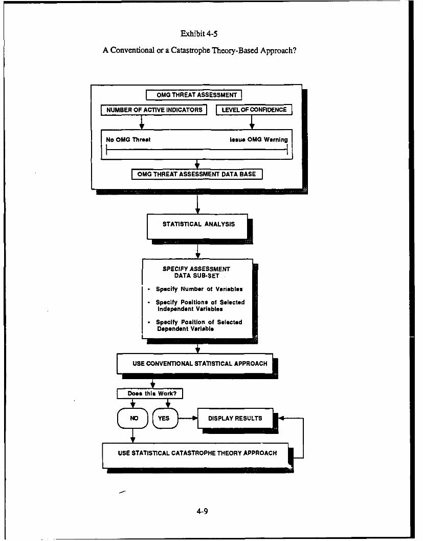
Exhibit 4-5

A Conventional or a Catastrophe Theory-Based Approach?


NUMBER OF ACTIVE INDICATORS LEVEL OF CONFIDENCE


OMG THREAT ASSESSMENT DATA BASE

STATISTICAL ANALYSIS

SPECIFY ASSESSMENTDATA SUB-SET

•Specify Number of Variables

" Specify Positions of SelectedIndependent Variables

Specify Position of SelectedDependent Variable

USE CONVENTIONAL STATISTICAL APPROACH

Does this Work?

NO YES DISPLAY RESULTS


4-9

increases the distribution of the test statistic converges to the chi-square distribution. Thedegrees of freedom for this chi-square statistic is the difference in the degrees of freedom forthe two models being compared, i.e., 2v+2. Sufficiently large values of this statistic indicatethat the cusp model has a significantly greater likelihood than the linear model.

Even if the first test shows that Equation (2) is superior to (1), the correct model may stillnot be the cusp catastrophe model. This can happen if the estimate for D is not significantlydifferent from zero, which it must be for the right hand side of Equation (2) to be a cubicpolynomial in Y. If D were zero the prediction equation for Y would read like this:

Y = C( ) A(X)/B(X). (5)

This is clearly not a catastrophe model, since for each value of X there is precisely one value ofY (which is infinite whenever B = 0). The second test for the adequacy of the cusp model is,therefore, a comparison of D with zero. As it turns out, D must be positive for a PDF of TypeN3 to be defined at all. Thus the appropriate test is a one-tailed t-test using the approximatestandard error of D. The degrees of freedom for this tct is the sample size less the remainingdegrees of freedom of the cusp model after D has been fixed at zero, i.e., N-3v-3.

Even if the model passes both of the preceding tests, it can happen that the onlycoefficients of the factors A and B which are significantly different from zero are the constantsA0 and B0. When this happens it is fair to say that the PDF of Y is indeed Type N3, but thatthe variables (if any) which cause this density to shift between bimodal and unimodal have notbeen included in the given list of independent variables. In this case the factor C determinesthe slope of the flat response surface. If the PDF is bimodal then there are two parallelresponse surfaces.

Lastly, it may happen that both of the above tests may yield positive results for the cuspmodel, implying that the cubic polynomial in Equation (2) is correct, while none of theobserved values for X lie in the bimodal zone! In this event the location of the bimodal zone isonly known by extrapolation from the given data. Since extrapolation is notoriously unreliablein statistical work, it is reasonable to require that some observations of X lie within the bimodalzone, while others lie outside. To assist the user in perceiving the estimated distribution of thedata within the plane spanned by the asymmetry and bifurcation factors, the cusp surfaceanalysis program shows this 2-dimensional distribution, with the bimodal zone highlighted.As a rule of thumb, it is desirable to have at least 10% of the observations fall within thebimodal zone. This constitutes the third test.

To summarize, the cusp catastrophe model may be said to describe the relationshipbetween a dependent variable Y and and vector X of independent variables if all of these threeconditions hold (Exhibit 4-6):




4-10

Exhibit 4-6

Criteria for Acceptance of the Cusp Catastrophe-Based Model


TESTS FOR EVALUATING ACCEPTABILITYOF CUSP CATASTROPHE MODEL

ASYMPTOTIC CHI-SOUARE TEST

~To determine whether the likelihood thata statistical cusp model Is a better fit for

the data then a linear model

CUBIC TERM ANALYSIS

---i To determine If the coefficients for the cubicterm and at least one of the other coefficients

are significantly different from zero

DATA LOCATION REVIEW

~To determine if at least 10 percent of thedata points of the estimated model are

located in the bimodal zone

SIF CRITERIA ARE SATISFIED


4-11

4.5 MAKING PREDICTIONS

In the literature on applications of catastrophe theory there are two distinct ways ofcalculating predicted values from a catastrophe model. In the Maxwell Convention thepredicted value is the most likely value, i.e., the position of the highest mode of the probabilitydensity function. In the Delay Convention a mode is also the predicted value, but it is notnecessarily the highest one. Instead, the predicted value is the mode that is located on the sameside of the antimode as the observed value of the state variable Y. Thus the delay conventionuses as its predicted value the equilibrium point towards which the equivalent dynamicalsy--tem would have nmoved. This is the convention most commonly adopted in applications ofcatastrophe theory, but there are circumstances in which the Maxwell convention is theappropriate one (Exhibit 4-7).

The cusp surface analysis program calculates the predictions made under each conventionfor each datum, and from these it derives a number of statistics and graphs to aid the user inevaluating the quality of the predictions made under each convention, as follows:

Modes and Antimodes: The estimated factors and modes and antimodes of the dataare presented to the user in tabular form.

Delay-R 2: This statistic is simply the estimated value of the quantity 1-(errorvariance)/var[Y], in which the errors are based on predictions of the delay rule.Although it is analogous to the multiple-R2 of regression analysis, there are severalimportant differences which are discussed below.

Maxwell-R 2: This is the corresponding statistic for the predictions of the Maxwellrule.

Error Histogram: This graph depicts the distribution of the errors made under thedelay rule. Also provided on this page are the mean and standard deviation of thisdistribution. These statistics are also known as the bias and standard error of estimate,respectively, of the estimates.

In multiple linear regression the estimates obtained by minimizing the mean squaredprediction error coincide with those obtained by maximizing the likelihood function. In cuspsurface analysis this is not the case, and therefore, the maximum likelihood estimates maxi-mize neither the Delay-R 2 nor the Maxwell-R 2. Further, neither of these statistics is evenguaranteed to be positive! Negative values occur when the cusp model fits so wretchedly thatits error variance actually exceeds the variance of Y.

Users of the Cusp Surface Analysis program are urged to try analyzing random data ofvarious types to learn more about how the program works. One such exercise, for example, isto create a set of data that are uniformly distributed about a linear trend. In this case theanalysis should yield the correct slopes in the linear factor and a positive bifurcation constant,indicating a model with two parallel prediction lines. Experimentation of this sort will alsodrive home the importance of having a sufficiently large sample size.

4-12

Exhibit 4-7

Cusp Surface Analysis: Making Predictions

CUSP SURFACE ANALYSIS: MakingPrdcin

Maxwell Convention: Delay Convention:

Predicted value is the most likely value, Predicted value Is the mode that is locatedthat is, the position of the highest mode on the same side of the entimode as the

of the probability density function observed value of the state variable


Calculate* the predictions mode under the Maxwell and

Delay conventions for each datum and derives statisticsand graphs to evaluate the quality of their predictions

KDy- S tatistic

L O rrHistogram

4-13

A particularly interesting experiment with the cusp surface analysis program can beperformed by generating data that fall exactly on the canonical cusp surface (i.e., which exactlysatisfy Equation (2), with C = 0). One would think that the analysis should reproduce thecorrect coefficients with no error, but this is not what happens. Recall that Equation (2) onlydescribes the deterministic model, and makes no statement about the conditional distribution ofthe random variable Y. On the other hand, the likelihood method makes the further assumptionthat this conditional distribution has a particular form, examples of which are depicted inExhibit 4-4. Notice that in Exhibit 4-4a, for example, the relative height of the two modeschanges very rapidly as the asymmetry factor increases. If the conditional distribution of Y inthe manufactured data set does not behave simlarly, then the cusp surface program will notyield the correct estimates. In fact, the maximum likelihood method will find the coefficientswhich best reproduce the empirical conditional distribution of Y, since this is roughly what itmeans to maximize the likelihood of a modeL

Each of the component variables of X contributes to each of the factors A, B, and C, andthe effect of each factor on Y depends on the values of the other factors. Thus it is hard tovisualize and understand the effect of any given variable. For this reason the cusp surfaceanalysis program displays a graph of the effect that each of the independent variables wouldhave on Y if every other variable were fired at its mean value.

Each graph shows the solutions to the cubic polynomial equation:

0 = (A0+AiX) + (B0+BiX)[Y - (CO+CiX)] - D[Y - (C0+CiX)]3, (6)

for a given i. The solutions are graphed for YI < 2.5 and IXI < 3.0, a region which includes allbut a tiny fraction of the observed values of X and Y. Thus even when there are threesolutions the graph may display only one or two, indicating that the others are far outside therange of commonly observed values.

As an example of such a graph, Exhibit 4-8 shows how the coefficient C in Equatio 1 (2)can affect the relationship between X and Y.

0 = -X + 3[Y - CX]- [Y - CX]3.

Notice how the number and location of the catastrophe points does not change as C changes,although the graph itself undergoes considerable deformation. This is characteristic of a"fiber-preserving" transformation (in this case the transformation is Y --> Y-CX).

4.6 A SAMPLE OUTPUT

A sample output from the cusp surface analysis program is presented in the final pages ofthis report Exhibit 4-9(a) shows the results of the computation of the mean and standarddeviations, correlation matrix, and the computation of log-likelihood values for the linear andcusp models on the basis of the information contained in a generic test data set. Exhibit 4-9(b)presents maximum likelihood estimates for the cusp model, an asymptotic chi-square andt-statistic values. Exhibit 4-9(c) presents the estimated correlations between the Alpha andGamma estimators and a table of predictions based on the cusp surface analysis. Exhibit4-9(d) presents P plot of the location of the data on the control space of the cusp catastrophe.Exhibit 4-9(e) presents a histogram plot of the residuals from the predictions of the delay rule.Exhibit 4-9(f) presents a plot showing the effect of variable 2 holding all others fixed at theirmean values and represents a "slice" through the cusp catastrophe manifold computed with theaid of the cusp analysis program. Exhibit 4-9(g) shows a similar type of plot for variable 3with the remaining variables held constant at their mean values.

4-14

Exhibit 4-8

71be Effect of Linear Factors

.............. ................................................. ....... .... ............ ............. ............................ .................. ........ ...... ............... .............. ............ ...... ...... ...... ........ ...... .......... ..... ...

...........

. . . . . . . . . . . . . . . . . . . . . .. . .... . . . . . . . . . . . . . . . . . . . . . . .. . . . . . . . . .

. . . . . .. . . .. . . . . . . .. . ..

.. . . . . . . . . . ... . . . . . . . . . . .

. . . . . .. . . . . . . . . .. . .. . . . . . . . .

The effect of X on Y in Equation 4 for C (-.50, -.25, 0,.25,.50)Note that the number andlocation of the catastrophe points does not depend on C.

4-15

Exhibit 4-9(a)

Sample Output from the Cusp Surface Analysis Program

Reading 3 variables from testdata

Positions of the variables (dependent variable last):2 3 1

Var Mean St.Dev

2 0.7742 0.58773 60.0303 28.2387

1 47.4545 25.7530

Correlation matrix:

2 3 12 1.00 0.55 -0.143 0.55 1.00 -0.31

1 -0.14 -0.31 1.00

Log-likelihood of the linear model: -45.1800

Standard linear regression coefficients:

Var Slope

2 0.0423 -0.329

Multiple R-squared: 0.095

Newton-Raphson algorithm, version of 1 Oct 1987

Step: 1: Log-likelihood: -45.180







•-- NEAR -*-

Step: 8: Log-likelihood: -33.354-NEAR **-


* NEAR ***

Convergence after i0 iterations.

4-16

Exhibit 4-9(b)

Sample Output from the Cusp Surface Analysis Program (Continued)

Cusp Surface Analysis, version of 4 October 1987.by Loren Cobb, Department of BiometryMedical University of South Carolina.Charleston, SC 29425.Phone 803-792-7575 for assistance.

Model: 0 - Alpha + Beta*(Y-Gamma) - Delta*(Y-Gamma)^3.

The conditional density of Y given X[1] .... X[v]:

f(YIX) - exp[ Psi + Alpha*Z + Beta*Z^2/2 - Delta*Z^4/4 J,

where Z - Y - gamma,

Psi - constant (with respect to Y),Alpha = A[0] + A[I]*X[1] + ... + A[v]*X[v],

Beta = B[0] + B[l]*X[1] + ... + B[v]*X[v],Gamma - C[0] + C[1*X[l] + ... + C[v]*X[v],

and v - 2 (in this analysis).

Maximum Likelihood Estimation for the Cusp Model:

Cases - 33Log-Likelihood - -33.3502

Standard coefficients, with t-statistics in parentheses:

Var Alpha Beta Gamma Delta

Const 0.131 (0.5) 3.326 ( 2.2) -0.146 (-1.5) 3.071 ( 2.7)2 0.438 (1.5) -0.318 (-0.4) -0.304 (-2.4)

3 -0.313 (-1.3) -1.829 (-2.1) 0.036 ( 0.4)

(Each t-statistic has 24 degrees of freedom)

Raw coefficients:

Var Alpha Beta Gamma Delta

Const 8.517e-3 1.151e-2 5.202e+l 6.981e-62 2.897e-2 -8.159e-4 -1.331e+I3 -4.306e-4 -9.768e-5 3.308e-2

Test for HO: Conditional densities are Type N2 (linear regression)versus Hl: Conditional densities are Type N4 (cusp regression)

>>>>>> Asymptotic Chi-square - 23.66 (df - 6) <<<

Test for HO: Delta - 0 (i.e. no cubic term)versus Hl: Delta > 0 (a one-tailed test)

>>>>>> t - 2.65 (df - 24) <<<<<<

4-17

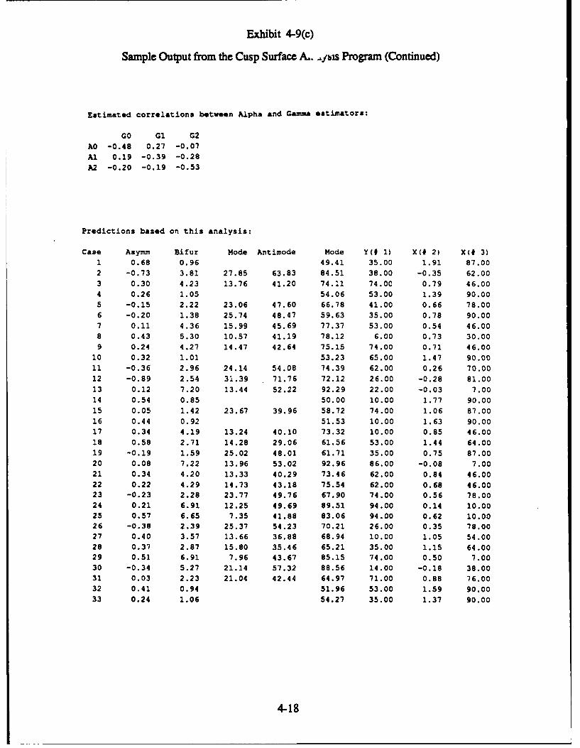
Exhibit 4-9(c)

Sample Output from the Cusp Surface A.. .Ibss Program (Continued)

Estimated correlations between Alpha and Gamma estimators:

GO Gi G2AO -0.48 0.27 -0.07Al 0.19 -0.39 -0.28A2 -0.20 -0.19 -0.53

Predictions based on this analysis:

Case Asymm Bifur Mode Antimode Mode Y(# 1) X(# 2) X(# 3)1 0.68 0.96 49.41 35.00 1.91 87.002 -0.73 3.81 27.85 63.83 84.51 38.00 -0.35 62.003 0.30 4.23 13.76 41.20 74.11 74.00 0.79 46.00

4 0.26 1.05 54.06 53.00 1.39 90.005 -0.15 2.22 23.06 47.60 66.78 41.00 0.66 78.006 -0.20 1.38 25.74 48.47 59.63 35.00 0.78 90.00

7 0.11 4.36 15.99 45.69 77.37 53.00 0.54 46.008 0.43 5.30 10.57 41.19 78.12 6.00 0.73 30.00

9 0.24 4.27 14.47 42.64 75.15 74.00 0.71 46.00

10 0.32 1.01 53.23 65.00 1.47 90.0011 -0.36 2.96 24.14 54.08 74.39 62.00 0.26 70.00

12 -0.89 2.54 31.39 71.76 72.12 26.00 -0.28 81.00

13 0.12 7.20 13.44 52.22 92.29 22.00 -0.03 7.00

14 0.54 0.85 50.00 10.00 1.77 90.00

15 0.05 1.42 23.67 39.96 58.72 74.00 1.06 87.00

16 0.44 0.92 51.53 10.00 1.63 90.0017 0.34 4.19 13.24 40.10 73.32 10.00 0.85 46.00

18 0.58 2.71 14.28 29.06 61.56 53.00 1.44 64.00

19 -0.19 1.59 25.02 48.01 61.71 35.00 0.75 87.0020 0.08 7.22 13.96 53.02 92.96 86.00 -0.08 7.00

21 0.34 4.20 13.33 40.29 73.46 62.00 0.84 46.00

22 0.22 4.29 14.73 43.18 75.54 62.00 0.68 46.00

23 -0.23 2.28 23.77 49.76 67.90 74.00 0.56 78.0024 0.21 6.91 12.25 49.69 89.51 94.00 0.14 10.0025 0.57 6.65 7.35 41.88 83.06 94.00 0.62 10.00

26 -0.38 2.39 25.37 54.23 70.21 26.00 0.35 78.0027 0.40 3.57 13.66 36.88 68.94 10.00 1.05 54.00

28 0.37 2.87 15.80 35.46 65.21 35.00 1.15 64.0029 0.51 6.91 7.96 43.67 85.15 74.00 0.50 7.0030 -0.34 5.27 21.14 57.32 88.56 14.00 -0.18 38.0031 0.03 2.23 21.04 42.44 64.97 71.00 0.88 76.00

32 0.41 0.94 51.96 53.00 1.59 90.0033 0.24 1.06 54.27 35.00 1.37 90.00

4-18

Exhibit 4-9(d)


Location of data in the control space:

Vertical axis: Bifurcation (splitting) factorHorizontal axis: Asymmetry (normal) factor

Asterisks: Bimodal zone

-5 -4 -3 -2 -1 0 1 2 3 4 5

5.0 0 0 0 0 0 0 0 0 0 0 0 0 0 0 0 0 0 0 0 0 0 5.0

4.5 0 0 0 0 0 0 0 0 0 0 3 0 0 0 0 0 0 0 0 0 0 4.5

4.0 0 0 0 0 0 0 0 0 0 1 0 3 0 0 0 0 0 0 0 0 0 4.0

3.5 0 0 0 0 0 0 0 0 0 0 0 1 0 0 0 0 0 0 0 0 0 3.5

3.0 0 0 0 0 0 0 0 0 0 1 0 1 0 0 0 0 0 0 0 0 0 3.0

2.5 0 0 0 0 0 0 0 0 1 1 1 1 0 0 0 0 0 0 0 0 0 2.5

2.0 0 0 0 0 0 0 0 0 0 0 2 0 0 0 0 0 0 0 0 0 0 2.0

1.5 0 0 0 0 0 0 0 0 0 0 3 0 0 0 0 0 0 0 0 0 0 1.5

1.0 0 0 0 0 0 0 0 0 0 0 1 6 0 0 0 0 0 0 0 0 0 1.0

0.5 0 0 0 0 0 0 0 0 0 0 0 0 0 0 0 0 0 0 0 0 0 0.5

0.0 0 0 0 0 0 0 0 0 0 0 0 0 0 0 0 0 0 0 0 0 0 0.0

-0.5 0 0 0 0 0 0 0 0 0 0 0 0 0 0 0 0 0 0 0 0 0 -0.5

-1.0 0 0 0 0 0 0 0 0 0 0 0 0 0 0 0 0 0 0 0 0 0 -1.0

-1.5 0 0 0 0 0 0 0 0 0 0 0 0 0 0 0 0 0 0 0 0 0 -1.5

-2.0 0 0 0 0 0 0 0 0 0 0 0 0 0 0 0 0 0 0 0 0 0 -2.0

-2.5 0 0 0 0 0 0 0 0 0 0 0 0 0 0 0 0 0 0 0 0 0 -2.5

-3.0 0 0 0 0 0 0 0 0 0 0 0 0 0 0 0 0 0 0 0 0 0 -3.0

-3.5 0 0 0 0 0 0 0 0 0 0 0 0 0 0 0 0 0 0 0 0 0 -3.5

-4.0 0 0 0 0 0 0 0 0 0 0 0 0 0 0 0 0 0 0 0 0 0 -4.0

-4.5 0 0 0 0 0 0 0 0 0 0 0 0 0 0 0 0 0 0 0 0 0 -4.5

-5.0 0 0 0 0 0 0 0 0 0 0 0 0 0 0 0 0 0 0 0 0 0 -5.0

-5 -4 -3 -2 -1 0 1 2 3 4 5

7 cases did not fit in the above figure.

>>>>>> Fraction of cases in bimodal zone: 0.788 <<Linear R^2 - 0.095 (Multiple regression)Delay R^2 - 0.695 (Attracting-mode zonvention)


* Negative R^2 values occur when the cusp model is worse than a constant.

4-19

Exhibit 4-9(e)


Histogram of residuals from predictions of the delay rule:(Units are standard deviations of the dependent variable.)

Y N-3.00 0 1-2.75 0 1-2.50 0 1-2.25 0 1-2.00 0 1-1.75 0 I-1.50 2 ##-1.25 0 1-1.00 1 1#-0.75 1 I#-0.50 5 i#####-0.25 7 1#######0.00 5 I#####0.25 5 1#####

0.50 5 I#####0.75 2 I##1.00 0 I1.25 0 11.50 0 11.75 0 12.00 0 12.25 0 1

2.50 0 12.75 0 13.00 0 1

Error Mean - -0.116Error St.Dev - 0.553

4-20

Exhibit 4-9(f)


Effect of variable 2, holding all others constant at their mean values.

-3 -2 -1 0 1 2 3.. ++++++++++++++++++++++ +++++.

2.5 + + 2.52.4 + + 2.42.3 + + 2.32.2 + + 2.22.1 + + 2.12.0 + + 2.01.9 + + 1.91.8 + + 1.81.7 + * + 1.71.6 + * + 1.61.5 + * + 1.51.4 + * + 1.41.3 + * + 1.31.2 + * + 1.21.1 + * + 1.11.0 + o * + 1.00.9 + 0 * + 0.90.8 + o * + 0.80.7 + o * + 0.70.6 + 0 * + 0.60.5 + 0 * + 0.50.4 + * + 0.40.3+ o * + 0.30.2 + o * + 0.20.1 + 0 * + 0.10.0 + o + 0.0

-0.1 + o + -0.1-0.2 + o + -0.2-0.3 + o + -0.3-0.4 + o + -0.4-0.5 + 0 + -0.5-0.6 + * 0 + -0.6-0.7 + * o + -0.7-0.8 + * 0 + -0.8-0.9 + * o + -0.9-1.0 + * 0 + -1.0-1.1 + * 0 + -1.1-1.2 + * o + -1.2-1.3 + * * + -1.3-1.4 + + -1.4-1.5 + + -1.5-1.6 + + -1.6-1.7 + + -1.7-1.8 + + -1.8-1.9 + + -1.9-2.0 + + -2.0-2.1 + + -2.1-2.2 + + -2.2-2.3 + + -2.3-2.4 + + -2.4-2.5 + + -2.5

...............................................................

-3 -2 -1 0 1 2 3

M ode symbol

o Antimode symbol 42

Exhibit 4-9(g)


Effect of variable 3, holding all others constant at their mean values.

-3 -2 -1 0 1 2 3

2.5 ............................................ +.2.5

2.5 + + 2.5

2.4 + + 2.42.3 + + 2.32.2 + + 2.22.1 + + 2.1

2.0 + + 2.0

1.9 + + 1.91.8 + + 1.8

1.7 + + 1.71.6 + + 1.6

1.5 +* + 1.51.4 + * + 1.41.3 + * + 1.31.2 + * + 1.21.1 + * + 1.11.0 + * + 1.00.9 + * + 0.90.8 + * + 0.80.7 + * + 0.70.6 + * + 0.60.5 + * + 0.50.4 + * + 0.40.3 + * + 0.30.2 + o + 0.20.1 + o + 0.10.0 + 0 + 0.0

-0.1 + 0 + -0.1-0.2 + o + -0.2

-0.3 + o + -0.3-0.4 + * + -0.4-0.5 + * + -0.5

-0.6 + * + -0.6

-0.7 + * + -0.7-0.8 + * + -0.8-0.9 + * + -0.9-1.0 + * + -1.0-1.1 + * + -1.1

-1.2 + * + -1.2-1.3 + * + -1.3-1.4 + * + -1.4-1.5 + * + -1.5-1.6 + * + -1.6-1.7 + * + -1.7

-1.8 + * + -1.8-1.9 + + -1.9

-2.0 + + -2.0

-2.1 + + -2.1

-2.2 + + -2.2

-2.3 + + -2.3-2.4 + + -2.4

-2.5 + + -2.5...............................................................

-3 -2 -1 0 1 2 3

• Mode symbolo Antimode symbol 4-22

SECTION 5. USING THE IWCAT SYSTEM

The IWCAT effort has investigated the use of catastrophe theory and related mathe-matical techniques as a methodology to support the activities of indications and warning (I&W)analysts. Prototype software, that implements these techniques in a manner that recognizes thatI&W analysts are not mathematicians and therefore require appropriate non-mathematical userinterfaces so that mathematical operations are performed automatically, has been produced.The following section describes how the IWCAT system has been used with OperationalManeuver Group (OMG)-related indicators to determine the likelihood that particularcombinations of these indicators reflect the formation of an 0MG.

The IWCAT software runs on an IBM-AT class computer and permits the analysis of theresponse of I&W analysts and others to indicators associated with a specific I&W-relatedsituation. Synectics, in collaboration with the government, has determined that the conditionsunder which an OMG is formed from an otherwise "normal" pattern of military advance are ofsufficient interest to the government to warrant its selection as the appropriate "I&W situation"as specified in the IWCAT statement of work.

5.1 STATISTICAL ANALYSIS AND CATASTROPHE THEORY

The IWCAT system presents its users with sets of OMG-related indicators and asks themto assess whether or not the information that they contain reflects the formation of an OMG.These assessments are analyzed with a statistical procedure that performs both a standard lineartype of analysis and a nonlinear, cusp catastrophe based, analysis in order to determine whichtechnique provides the best "fit" for the data.

The cusp catastrophe model provides a description of systems which exhibit nonlinearand ambiguous behavior and of situations in which changes in the values of system variablescan give rise to either gradual or sudden changes in behavior under different circumstances.Such behavior appears to be associated with indications and warning and its nature can only beexamined with great difficulty, if at all, with the aid of the more classical statistical approachesinvolving normal distributions and with linear regression techniques.

5.1.1 KEY VARIABLES

The catastrophe analysis involves the identification of key system variables and the use ofthese as factors in the statistical procedures. Review and analysis of the I&W environment hasled the IWCAT project team to the identification of the following two major key input variables(called control factors) and one major output variable (called a behavior variable) which candescribe at least some of the major features of the activities performed by I&W analysts.

1. The control factors represent the inputs to the process of I&W analysis. At this time,the IWCAT project team has selected two control variables which they have describedas the number of active indicators and the level of confidence to represent theseinputs. The "number of active indicators" variable represents the number ofindicators which are activated when the analyst makes a judgment. Additional factors

5-1

including weather, time of day, sequence type, and scenario type have also beenincluded as potential control factors, as described below. The "level of confidence"variable represents a measure of the degree to which the set of indicators presented tothe analyst is considered to reflect the actual conditions of a situation of interest.

2. The behavior variable represents the result of the I&W process. The IWCAT projectteam has tentatively named this variable the analyst's perception of OMG threat sinceit represents the perception of the I&W analyst of the likelihood that a particularmilitary situation reflected in the set of indicators presented to the analyst representsthe formation of an OMG from an apparently "normal" pattern of military advance,for example.

During each assessment activity, a selection of test data sets, each with different numbersof active indicators and level of confidence and related information, are presented to the usersof the IWCAT system and they are asked to assess the level of OMG threat as reflected in thesedata by indicating a position on a scale line. These assessments and the input information formthe basis of the OMG Threat Assessment data base. The results for each individual participantare tabulated, recorded, and analyzed as described in below, in order to determine whether thedata can be described with the aid of a linear model, or whether the data could be describedmore appropriately with the aid of a nonlinear model based on the cusp catastrophe.

5.2. SYSTEM REQUIREMENTS

5.2.1 HARDWARE

The IWCAT system is designed to run on any IBM-AT compatible computer equippedwith a mathematics coprocessor and a color monitor. The program can also print out theresults of the statistical analysis onto printers of the IBM Proprinter class.

5.2.2 SOFTWARE

The IWCAT software consists of a compiled computer program IWCAT.COM containedon a 5.25 inch floppy disk which contains all the special utilities required for running theIWCAT system.

5.2.3 GETITING STARTED

Insert the IWCAT disk into the disk drive and turn the power on. When prompted by thecomputer with the prompt symbol, >, enter the symbol A (thus: >A) and then enter whenprompted: > IWCAT. The IWCAT system will then be ready for use and the main menu canbe accessed by pressing the "enter" key and will available for user selection.

5-2

5.3. THE IWCAT SYSTEM

The IWCAT system provides menu-driven access to the series of facilities displayed inExhibit 5-1 and outlined below.

5.3.1 MENU DISPLAY OVERVIEW

Thc. IWCAT Menu provides the user with access to the various components of theIWCAT system (Exhibit 5-1). Access to these components is obtained by typing the requiredoption code number when instructed by the program.

Personal information has to be entered under menu item "2" before proceeding to theremainder of the system since this information is used to identify the data files created duringuse of the IWCAT system. The following selections are available to the user:

> 1 Provides a description of the IWCAT system and presents the text of the three

scenarios which provide the context for the OMG threat assessment activities.

> 2 Allows entry of the necessary identifying personal and/or code information.

> 3 Makes a test file of indicator data for user assessment.

> 4 Permits the user to practice indicator assessment and data entry.

> 5 Enables the user to perform assessments of the test data set.

> 6 Creates a file for analysis with the identification of primary and secondaryindicators.

> 7 Performs the cusp analysis.

> 8 Terminates the use of the IWCAT system.

5.3.2 READ ABOUT THE PROGRAM

Menu option "1" ("Read About the Program") (Exhibit 5-2) provides the user with accessto a text file that outlines the properties of catastrophe theory, some of the properties of OMGsand the OMG indicators, describes the nature of the IWCAT program and the tasks that theuser will be asked to perform and other details of the analytic environment. The I&W indicatorsets will be presented against the background provided by one of three scenarios, reflectingconditions characterized as:

1. Treaty Obligation

2. Friendly Ally

5-3

Exhibit 5-1

IWCAT System Overview Menu Display

Enter an Option and Press "Return"

1. Read about the program

2. Enter Information about yourself

3. Make a Test File

4. Practice Session

5. Take the Test

6. Make a File for Analysis

7. Perform Cusp Analysis

8. Quit

5-4

Exhibit 5-2

IWCAT System Overview Menu Display, Option 1: Read About the Program


( 1. Red about the program


3. Make a Test File

4. Practice Session

5. Take the Test



8. Quit

1. Red ebout the Progrem

Option "1" presents a text file to the userdescribing the IWCAT computer system,Including:

* Types of activities to be performed.

" Nature of analyst data sets, Indicators,and knowledge development activities.

" Text of "Treaty Obligation," "FriendlyAlly," and "Third Party Hostilities"

Scenarios.

" Nature of Statistical Analysis to beperformed.

5-5

3. Third Party Hostilities

The material contained in the text files accessed under option "1" is self explanatory.

5.3.3 ENTER INFORMATION ABOUT YOURSELF

Menu option "2" ("Enter Information About Yourself") (Exhibit 5-3) asks the user toenter items of personal information which serves as the basis for creating an identification codefor the user-generated data sets.

Under option "2," the user enters the following items of information:

1. First Name (Amnopq, for example).

2. Family Name (BCDEFGHijk, for example).

3. Number of years as an analyst (XX, for example).

The first letter of the first name and the first seven letters of the family name are used tocreate the data file for cusp analysis after the primary and secondary indicators have beenidentified at the completion of the testing sequence. Thus the above entries would create a datafile named: ABCDEFGH.CUS, for example.

In the case of multiple uses of the IWCAT system by a single user, theuser should be aware that entry of the same items of personal information for asubsequent use will cause the creation of a data file which will obliterate apreviously created file with the same identifier. Under such circumstances,some form of personal coding scheme should be adopted for each IWCATsystem use.

Completion of these data entry activities is signaled by pressing the "Esc" key once.

5.3.4 MAKE A TEST FILE

Menu option "3" ("Make a Test File") (Exhibit 5-4) permits the user to generate a newtest data file consisting of fifteen sub-files each of which is associated with one of the threetypes of scenario (Treaty Obligation, Friendly Ally, or Third Party Hostilities) and one of fivedifferent patterns of indicator sequences. The data file is given a label based on the personalinformation entered under option "2." When prompted, the user enters an appropriate identifierlabel, the user's initial and the first seven characters of the family name, or a user-selected codeis recommended for this purpose (Exhibit 5-5). Entry of this information triggers the creationof a test data file and the creation of such a test data file is indicated by a self explanatorysequence of displays.

5-6

Exhibit 5-3

IWCAT System Overview Menu Display, Option 2: Enter Information About Yourself

Enter an Opion and Press "Return"


Enter Information about yourself

&. Make a Test File

4. Practice Session

5. Take the Test



8. Quit


Option "2" asks the user to enter the

following Items of personal information:

" First name: (eg: Amnopq)

• Family name: (eg: BCEDFGHIk)

" Number of years as an analyst: (eg: XX)

The first letter of the first name and thefirst seven characters of the family nameare used as Identifiers of the data filescreated during the use of the IWCAT system.

The above entries would create a file name:ABCDEFGH, for example.

5-7

Exhibit 5-4

IWCAT System Overview Menu Display, Option 3: Make a Test File

Enter an Option and Press Return



4. Practice Session

5. Take the Test



8. Quit

3. Ma~ke s Test File

Option "3" permits the user to generate a newtest data file consisting of fifteen sub-files,each of which Is associated with one of the threescenarios (Treaty Obligation, Friendly Ally, orThird Party Hostilities).

The data file Is given a label (usually consistingof the user's Initial and the first seven Initialsof the family name provided by the user).

Sample File Name: ABCDEFGH.PAT

The data file: ABCDEFGH.PAT can then beused In the testing environment by typing Inits name when requested by the computerduring exercise of Option "5."

5-8

Exhibit 5-5

Making a Test File

OPTION 3: MAKE A TEST FILE

Pattern File Name: ABCDEFGH.PAT

Getting Sequence 1, 2, ... , 15

Getting Pattern 1, ..., #

5-9

5.3.5 PRACTICE SESSION

Option "4" ("Practice Session") (Exhibit 5-7) permits the user to gain experience in theprocesses of assessing the levels of OMG threat represented in the IWCAT data sets andrecords this information within a test data file in a manner that is identical to the way in whichOMG threat data will be assessed and this information is entered into the computer during theactual testing process.

The system will ask the user to specify the practice data set. A practice data set labeledPRACTICE.PAT has been provided for practice purposes and the user should enter thisidentifier when prompted by the computer. The system asks the user to specify the number ofscales to be placed on the OMG Threat Assessment Indicator ine (Exhibit 5-7). The followingprompt message appears:

number of scale divisions? 2/4

The user will select one of these options by typing in either 2 or 4, producing the display:

number of scale divisions? 2/4 2, for example.

5.3.5.1 Practice Data Presentation

The practice data set (PRACTICE.PAT) provides a series of data screens each ofwhich contain the following data elements (Exhibit 5-8):

1. An array of 10 OMG-related indicators (Exhibit 5-9). Active indicators are indicatedby the presence of a white colored rectangle.

2. Type of weather information is presented in text format.

3. Time of day information is presented in text format.

4. Level of confidence information is presented in numerical format with numbersranging from 0 (zero level of confidence in the reliability of the data) to 100(absolute confidence in the reliability of the data).

5. Scenario type information (Treaty Obligation, Friendly Ally, or Third PartyHostilities) presented in text format.

The data is presented in a series of blocks with each block of data corresponding to onetype of scenario. Thus, the practice sequence can begin with the presentation of a screenidentifying a series of data sets relating to a "Treaty Obligation" scenario. These data areassessed for OMG threat level (see section 5.3.5.2) and this assessment recorded by pushingthe "Enter" key.

5-10

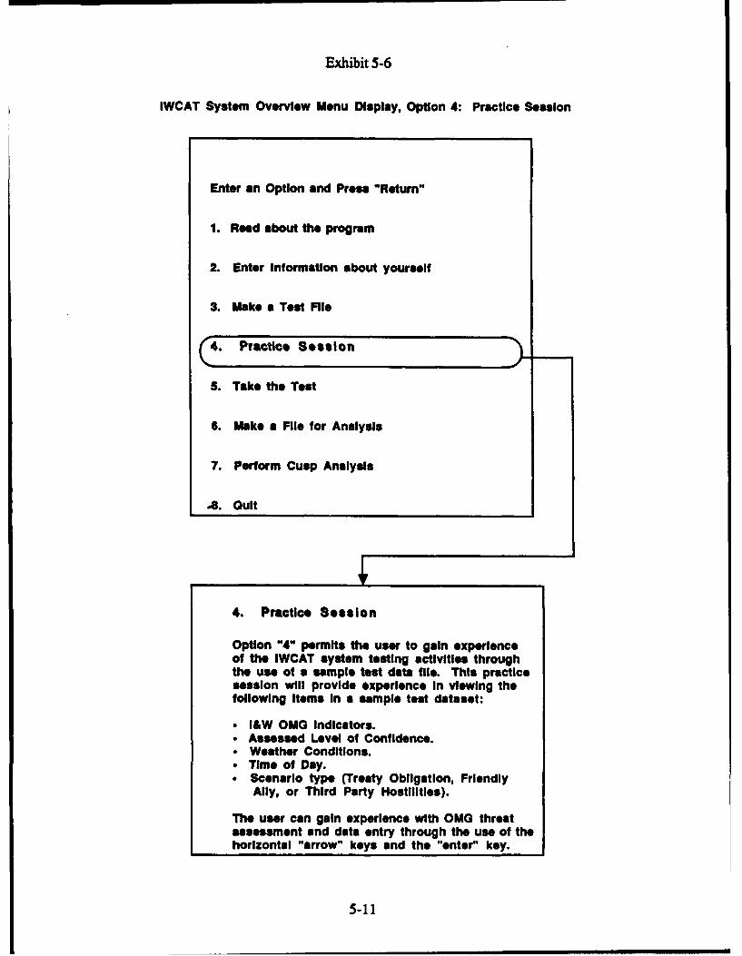
Exhibit 5-6

IWCAT System Overview Menu Display, Option 4: Practice Session




3. Make a Test File

4Practice Session

5. Take the Test



.8. Quit

4. Practice Session

Option "4" permits the user to gain experienceof the IWCAT system testing activities throughthe use of a sample test data file. This practicesession will provide experience In viewing thefollowing Items In a sample test dataset:

" I&W OMG Indicators." Assessed Level of Confidence." Weather Conditions." Time of Day.* Scenario type (Treaty Obligation, Friendly

Ally, or Third Party Hostilities).

The user can gain experience with OMG threatassessment and data entry through the use of thehorizontal "arrow" keys and the "enter" key.

5-11

Exhibit 5-7

Entering 0MG Assessment Practice Data

Number of Scaos 2/4 2

No 0MG Treel bsus 0MG Wernkng

(Arrow key ".c") '-II- (Arrow key ""

5-12

Exhibit 5-8

Practice Session Activities

-1 Enter OptionSww option 10 1. Read ...

2. Enter ...3. Make ...

Enter 3 Pradoe Data 4.Practice...

sag S. Take ...6. Make ...7. Perform ...8. Quit

Start of PractioeSeWence

Treaty Obligation

IlLn!tj

Too

End of PracticeFLO-C Sequenoe

Treaty Obligation

FT-T

----------Enter

Start of PracticeSO*XW= Enter OptionFriendly Ally End reclice 1. PAW ...

of P 2. Enter ...3. Make ...4. Practioe ...S. Take ...6. Make ...7. Performa. Ouit ...

5-13

Exhibit 5-9

Practice Data Display

Intensified Reconnaissance and Intelligence [ Weather



Timeincreasing Air Support Night


Armor Assembly Areas Within 30-50 km. of the FLOT FLevel of

Combat Enginer eConfidence

Traffic Control and Lane Clering n Tot

Electronic Silence Obligation

Electronic Countermesures and Deception


5-14

5.3.5.2 Practice OMG Threat Assessment

The user is asked to assess the level of OMG threat reflected in the OMG-related indi-cators and enter this information into the computer with the aid of the indicator scale positionedin the lower portion of the computer screen (see Exhibits 5-7, 5-8, and 5-9).

This task is performed with the aid of the horizontal arrow keys "<" and ">" whichpermit the user to position the blinking indicator arrow at a position of the OMG ThreatAssessment line that corresponds to the level of OMG Threat that the analyst perceived as beingreflected in the data presented on the screen (Exhibit 5-7).

Completion of each assessment is signaled by pushing the "Enter" key which enters theresults of the assessment into the OMG Threat Assessment data file. The end of each block ofdata is indicated by a self-explanatory display (Exhibit 5-8). The next block of data is accessedby pressing the "Enter" key. Completion of the complete practice sequence is indicated by thereturn to the menu display for further option selections,

5.3.6 TAKE THE TEST

Option "5" ('Take the Test") (Exhibit 5-10) permits the user to assess the levels of OMGthreat represented in the IWCAT data sets and records this information within a test data file.

Option 5 ("take the test") should always be accessed before options 6 ("Make a File forAnalysis") and 7 ("Perform Cusp Analysis"), although these activities can be performed duringdifferent sessions of activity.

On selection of option 5, the system asks the user to specify the number of scales to beplaced on the OMG Threat Assessment Indicator line (Exhibit 5-11). The following promptmessage appears:

number of scale divisions? 2/4

The user will select one of these options by typing in either 2 or 4, producing the display:

number of scale divisions? 2/4 2, for example.

The system automatically presents the first test data set for analyst assessment.

5.3.6.1 Test Data Presentation

The test data set provides a series of data screens each of which contain the followingdata elements (Exhibit 5-11):

1. An array of OMG indicators (Exhibit 5-12), with white squares in the arraysignifying which of these indicators is active.

2. Type of weather information.

3. Time of day information.

5-15

Exhibit 5-10

IWCAT System Overview Menu Display, Option 5: Take the Test



2. Enter information about yourself

3. Make a Test File

4. Practice Sesion

5.Take the Test



a. Quit

S. Take the Test

Option "5" provides facilities for capturing theanalyst's perceptions of the level of OMG Threatas presented In a test dataset with the followingentries:

" I&W OMG Indicators." Assessed Level of Confidence." Weather Conditions." Time of Day." Scenario Type (Treaty Obligation, Friendly

Ally, or Third Party Hostilities).

This assessment Is Indicated through the use ofthe horizontal "arrow" keys and recorded bypressing the "enter" key.

5-16

Exhibit 5-11

Enter 0MG Test Data Assessments

Number of Scaies 2/4 2

No 0MG Thread Imue 0MG Warnng

(Arrow key "c)4 S (Arrow key m"

Enter Data]

5-17

Exhibit 5-12

OMG Test Data Presentation

Intensified Reconnaissance and Intelligence Weather



Time

Increasing Air Support Night


Armor Assembly Areas Within 30-50 km. of the FLOTLevel ofI Confidence 80


Traffic Control and Lane Clearing ! Tet

TreatyElectronic Silence Obligation

EetoiConermeasures and Deception

No OMG Threat lase OMG WarningI I

5-18

4. Level of confidence information.

5. Scenario type information (Treaty Obligation, Friendly Ally, or Third PartyHostilities).

As in the case of the practice session, the data is presented in a series of blocks with eachblock of data corresponding to one type of scenario. Thus, the practice sequence can beginwith the presentation of a screen identifying a series of data sets relating to a "TreatyObligation" scenario. These data are assessed for OMG threat level (see Section 5.3.6.2) andthis assessment recorded by pushing the "Enter" key on the keyboard.

5.3.6.2 0MG Threat Assessment

The user is asked to assess the level of OMG threat reflected in the OMG-relatedindicators and enter this information into the computer with the aid of the indicator scalepositioned in the lower portion of the computer screen (see Exhibits 5-11, 5-12, and 5-13).

This task is performed with the aid of the horizontal arrow keys "<" and ">" whichpermits the user to position the blinking indicator arrow at a position oi the OMG ThreatAssessment line that corresponds to the level of 0MG Threat that the analyst perceived as beingreflected in the data presented on the screen (Exhibit 5-12).

Completion of each assessment is signaled by pushing the "Enter" key which enters theresults of the assessment into the OMG Threat Assessment data file (Exhibit 5-13). The end ofeach block of data is indicated by a self-explanatory display. The next block of data is accessedby pressing the "Enter" key. Completion of the complete test sequence is indicated by thereturn to the menu display for further option selections.

5.3.7 MAKE A FILE FOR ANALYSIS

Option "6" ("Make a File for Analysis") (Exhibit 5-14) permits the user to separate theI&W indicators into "primary" and "secondary" categories to facilitate the analysis of the usergenerated OMG threat assessment data.

Option 6 ("Make a File for Analysis") should always be accessed after option 5 ("Takethe Test") and before option 7 ("Perform Cusp Analysis") although these activities can beperformed during different sessions of activity.

When option 6 is selected, the user is presented with a screen display (Exhibit 5-15) andasked to enter data indicating choice of the primary indicators by typing a "1" into the appro-priate positions. Completion of the task is indicated by pressin,, the "Esc" key once. This taskresults in the automatic creation of a data file with the label:

ABCDEFGH.CUS

This file is the one that the user will select during the cusp analysis activity (option 7) describedbelow.

5-19

Exhibit 5-13

0MG Threat Assessment Activities

-1 ~ Enter OptonSew Opion10 1 . Read ...

2. Enter ...3. Make ...

Ente 15 aft eclunoes4. Practice ...S. Take..6. Make..7. Perform..8. Quit..

EEnter

7.nPteor

Stall_______ of Seuent

Frindl Aly nte5Opio

Exhibit 5-14

IWCAT System Overview Menu Display, Option 6: Make a File For Analysis




3. Make a Test File

4. Practice Session

5. Take the Test

(6. Make a File for Analysis


8. Quit


Option "6" provides facilities for recordingwhich of the ten available i&W Indicators wereof the greatest importance to the analyst inassessing the level of OMG Threat.

The user Is asked to identify the most Important(or "primary") Indicators by placing a "1" in theappropriate location in the array of Indicatorsthat are presented on the computer display. Allother Indicators are deemed to be "secondary"Indicators.

Completion of this task leads to the creation of adata file with the following label: ABCDEFGH.CUS,which can be passed to the cusp program forstatistical analysis under option "7."

5-21

Exhibit 5-15

Making a File for Statistical Analysis

ANLSISOPTION 6: MAKE A FILE FOR ANALYSI

Intensified Reconnaissance and Intelligence

Concentration of Artillery Units In the FLOT Area


increasing Air Support

Dummy Coneentrations

Armor Assembly Areas Within 30-50 km. of the FLOT


Traffic Control and Lane Caering

Electronic Silence

Electronic Countermeasures and Deception

5-22

5.3.8 PERFORM CUSP ANALYSIS

Option "7" ("Perform Cusp Analysis") (Exhibits 5-16 and 5-17) provides access tofacilities for performing a statistical analysis of analyst OMG threat assessment.

Option 7 ("Perform Cusp Analysis") should always be accessed after options 5 ("Takethe Test") and 6 ("Make a File for Analysis"), although these activities can be performed duringdifferent sessions of activity.

Selection of option 7 causes the computer to display the request for a data file name (seeExhibit 5-15):

Data File Name:

Following the examples presented earlier, the user should type in the following:

Data File Name: ABCDEFGH.CUS

where ABCDEFGH is the user's name or code identifier (see Exhibit 5-3). The program willprint the following request:

Total Number of Variables in Input List:

The user should enter the number 11:

Total Number of Variables in Input List: 11

The program then asks for the number of variables to be used in the analysis. Here the usercan select which of the eleven variables should be passed to the cusp program for analysis.

Number of Variables to be used in this analysis:

The user now enters a number, which is "3" in the example illustrated in Exhibit 5-17 but morethan three variables can be used in the analysis, with the restrictions mentioned below.

Number of Variables to be used in this analysis: 3

The program then asks the user to identify the positions of the variables in the data fileABCDEFGH.CUS that will be used in the analysis.

Position of these dependent variables within the input list, with dependent variableLAST:

Here the user should enter the selected list. In the example shown in Exhibit 5-17, thefollowing entries are made:

1: 4 (enter)2: 10 (enter)3: 11 (enter)

The pattern number (position 1) or BOTH the number of primary andsecondary indicators (positions 2 and 3) AND the total number of indicators(position 4) should not be used together since this will produce irrelevantcorrelations, but BOTH "2"and "3" CAN be entered WITHOUT entering "4."

5-23

Exhibit 5-16

IWCAT System Overview Menu Display, Option 7: Perform Cusp Analysis




3. Make a Test File

4. Practice Session

5. Take the Test


C7. Perform Cusp Analysis

8. ouit


Option "7" provides facilities for performing astatistical analysis of analyst OMG ThreatAssessment files with the following type ofIdentifier: ABCDEFGH.CUS

The IWCAT system asks the user to specify thefollowing Information:

" File name (typically: ABCDEFGH.CUS)." Total number of variables In the .CUS file.- Number of variables to be used In the analysis.* Which variables are to be used, with the

dependent variable entered last.

The system performs the analysis and prints theresults In tabular and graphical formats.

5-24

Exhibit 5-17

Cusp Analysis Activities

OPTION 7:CUPALYI

Dds Fie Name: ABCDEFGH.CUS____ ___ ____ ___ ____ ___ ____ ___Variable List:

1. Pattern Number

Total Number of Variables in Input List ~ ]. 2. Number of Primary Indicators

________________________________3. Number of Secondary Indicatos

- 1~. OMGncTypatesmn

PostinsOf he Vrial ouWtnIput hast bee Scentrd toaTieyaedpep

With(b) Detpendentn neriabve LASTng again.oeLa

(I) Ao Ikiho no InraigWteaintr ate y

Convergence ~1 afdr Coeatnnsiodenchseee

afpthbwprinted to a fil e named "Cuspou

Q- Print CuspoutName of Ust Device EPRN]: pirResident part of PRINT InstalledC*:\IWCAT\CUSPOUT is currenly being printed

5-25

The statistical analysis program first fits a linear model to the user-generated data file andthen determines whether or not the cusp model provides a better fit to these data. The cuspanalysis program ceases when it is determined that the linear model is better than the cuspmodel.

ine sample information presented in Exhibits 5-18 to 3-24 are the result of the use of thestatistical program to analyze test data contained in a file named: "testdata." The cusp surfaceanalysis program begins by displaying the mean and standard deviations of the input variablesand the correlation matrix for these variables and also calculates the log-likelihood statistic andthe standard linear regression coefficients for a linear model (Exhibit 5-18).

The statistical program then iterates toward conditions that maximize the likelihood of thecusp model based on the observed data. The iterative scheme is based on a modified Newton-Raphson method. If the very first iteration yields a decrease in the likelihood function, theprogram immediately halts with a message indicating that the linear model is preferable to anycusp model (this is not a rare occurrence). Upon successful convergence to a condition thatmaximizes the likelihood function, the estimated coefficients of each factor are stored in a filelabeled CUSPOUT, for printing or review.

As iteration proceeds, the completion of each step in the process is signaled by theprinting of a hyphen ("-"). When the iterative process requires the use of special numericalintegration procedures, the following symbol ("+") is printed. Use of these special numericalprocedures signal that the convergence process is being undertaken with difficulty, and mightfail. One of several different messages can be printed out during the process of iterationtoward convergence (see Exhibit 5-15, for example).

1. Iteration can be halted if the cubic coefficient vanishes and it is not possible to form acusp-based model with the available data.

2. During the convergence processing, it may happen that the determination of a Hessianmatrix used in the computation becomes negative. This suggests the program ishaving trouble with achieving a suitable convergence, and that the attempt might fail.

3. Convergence may also fail if the process does not lead to a reduction of the log-likelihood value.

4. As convergence is approached, the program prints out the message "*** NEAR **"and when convergence is achieved, it prints out the following message:

Convergence after # iterations, please wait, output has been printed to a file named"CUSPOUT."

The user can now display the contents of the file labeled "cuspout" on the screen byresponding to the instruction:

> Type cuspout

A hardcopy of the file cuspout can be generated for review and analysis by respondingto the instruction (Exhibit 5-15):

> Print cuspout

5-26

Exhibit 5-18


thdata fiMe lestdta" with

•eading 3 variables free testdate poskOm at wal S as speW

Positions of the variables wdepeeient variable lasti:2 3

Vat Weon St.Oev2 0.7742 0.5877

3 60.0303 20.23871 47.4545 25.7530

Correlatieon .zr: C o matrix shows mogrre2 3 1-of reldimshiP betwee variables

2 1.00 0.51 -0.143 0.55 1.00 -0.31 Value of the o-1* lhood lor 8 in1 -0.14 -0.31 1.00

Lo;-likelihood of the lnear medel: -45.1000

Standard linear regression mfficients: j C " sotai r n e a

Va: Slope .M ssa we"s2 0.0423 -0.323 LMI sq ~qndvlI'Ziple I-squared: 0.005 JSgs theta Wow I o he

Uevmon*~-hp~ algorithi. woe:io of i Oct it7

Step: 2: L ;-likelihood: -42.235 UseofNwwW-R0on Mgodtn to--daato ----eu(-) model

"'e.=: 3: L.o;-±Ijkelshod: -40.3

ite: 4: L*;-Xike1.hoo¢: -35.721

Step: 5: L=g-ljkelihooc: -34.197

Ite=: 4: Lo;o-ikelLhooc: -33.53C

Step: 1: L:;-likelhood: -33.376

Step: O: Log-like ihood: -33.354** IAL ...

Sftep: 9: L:q-! k*e'ho=d: -33.35:

Convergenoe afte 10 iterations toConve*rqence ater 10 Itea:tions. a iowe iog.Ii9ihoodw vakmm o te

..- a bw mode mows th om s modeto be a better fit for the data

5-27

5.3.8.1 Testing the Model

The parameter estimates reported by the cusp surface analysis program are useful forgenerating predictions, but their values indicate nothing about their statistical significance.Therefore the program also reports an approximate t-statistic for each coefficient, with N-3v-3degrees of freedom. These can be interpreted in the usual fashion: magnitudes in excess of thecritical value indicate that the coefficient is significantly different from zero, at the specifiedsignificance level (remember that these t-statistics are only approximate). Of course, thesestatistics can also be misinterpreted in the usual ways too. For example, it is a mistake to payattention to any of these values unless the overall model has passed all of its tests foracceptability.

Cusp surface analysis offers three separate tests to assist the user in evaluating the overallacceptability of the cusp catastrophe model. The first test is based on a comparison of thelikelihood of the cusp model with the likelihood of the linear model. The test statistic is an"asymptotic chi-square," which means that as the sample size increases the distribution of thetest statistic converges to the chi-square distribution. The degrees of freedom for this chi-square statistic is the difference in the degrees of freedom for the two models being compared,i.e., 2v+2. Sufficiently large values of this statistic indicate that the cusp model has asignificantly greater likelihood than the linear model. The cusp catastrophe model may be saidto describe the relationship between a dependent variable Y and vector X of independentvariables if all of these three conditions hold:




The results of performing these tests are transferred to the "cuspout" file and are dis-played for the test data file "testdata" in Exhibit 5-19, for example.

The data used in the cusp analysis, including the dependent and independent variables,the cusp estimation of the values of the modes and antimodes predicted by the cusp analysisprogram, and the position of each data point with respect to the axes of the cusp control spaceare displayed in Exhibit 5-20.

The computed positions of the data points from the "testdata" file are displayed in Exhibit5-21. The analysis reveals that 78.8 % of the test data cases fall within the bimodal zone andthat 7 of the 33 cases are located in coordinate positions outside the boundary of the figure.These latter 7 cases are, however, still part of the cusp analysis. The R2 statistics suggest thatthe data is best fitted by a delay (or attracting-mode) convention transition rule (Exhibit 5-21).

The histogram of residuals (Exhibit 5-22) provides an indication of the degree to whichthe test data can be fitted to the cusp model. Exhibit 5-23 presents a plot showing the effect ofvariable 2 holding all others fixed at their mean values and represents a "slice" through the cuspcatastrophe manifold computed with the aid of the cusp analysis program. Exhibit 5-24 showsa similar type of plot for variable 3 with the remaining variables held constant at their meanvalues.

5-28

Exhibit 5-19


Cusp Surface Analysis. versies of 4 October 1967.by Loren Cobb, epartment of BiometrysOdicai University of South Carolina.

Cahrleston. SC 29425.Phoa. g03-792-7SS for assistance.

IN ihs Uw tw ftn of the fil:sdidel: 0 - Alpha . Mea(tY-Ga ] - Delta' (%N) 3.C.

Te mnditional density of Y liven XZI).....XIVI:

fTIXI - exp[ Psi # Alpha*Z * Beta*Z'2/2 - Delta2*4/4 1.

ftere 2 * Y - gam&.

PsA - constant (with respect to T).Alpha - AIO) + AII]*XII] * ... * AIV(-X(vI,seta - s01 # 3rc.x:: 1 ... * Dv)oxlvj,

Gascs - CIO) * CIX|*XIi . * C~vloX(vl.

And v - 2 (in this ar.'ysial.

Ia=l&, Likelihood Estiza2lon fox ta Cusp; ).=el:

The A" Variabl a the NormalCases - 33 Fedor (at "ght-anlos" to the cusp)

Iag-Lkelihosd - -33.31:2

The Boa Vauldise is th SplittingItanda:d eoeficAe.ts. v":h t-statistles i*.n Faentheses: Falor r(Opw up 9w atJsp"

Var Alpha beza Gs?. Delta o Te Gamma vanaa is a Unear-- t------- ---- ------ --- for that can Meiearty displace the

Const 0.131 C.5) 3.324 ( 2.2) -0.:46 (-1.-2 3.07l (2.') cuspsuulace

2' 0.431 1!.5) -0.3180 !-C.4) - .: (-2.41

3 -0.313 (-1.3) -i.929 (-2.11 o.::,f ( 04) TheltaVariablreprese tsthecoefficient multiplyig the cubc or

MEach t-statiste has 24 degrees o fre.wd-) *cusp" term

Raw eoe;iClents:

Va. A -Iha. be- Gasm :Olt&

onst. 1.517e-1 1.IS:e-2 5.2 02*-! f.9810e-1

2 2.1;?e-2 -6.1! e-4 -1.331e-13 -4.306-4 -9.II1e-S 3.306a-2

Test fc: FZ: C:nc;tion:: dons':lts are 7ype :2 (Ulinea. roqasslol

ve.s;s hI: Cor.r;tiona: densi:tes are 7yp. N4 icus: :eq:ess~on)

311 - - - AymteicCh-sua*- 23.64 (df - 6) ~~(ccc C sweM slw um-

PopeC is$ am- a.: s:l

5-29

Exhibit 5-20


-041.40 0.21 40.O1£1 0. 5O -. 3l -4.50

00 -0.10o -0.1 -. 5.

For fm 33 set of data elemenm inthe "ostdata file, the cusp analysisprogram estmates th followingproperties:

Position with respect to the Normaland Splitting Factor Axes

Positins of the mode(s) and antmooeof the property distribution functionwith regard lo the behavior variable

gme mimia wl~meo ,e Ii 340 Ii *. I_______________________ Im..3 -0.1 ?l Ll 11, A 102 04.1 3 It.00 .t.11 i .,i3 0.30 0.32 1.I. 10 41. 0 14.1 24.00 0.1 40.00

0 -4.11 3.1* 3.00, 4. 04.70 41.00 0.04 10 Th. program also prlnm theI0 -..1 .30 1.14 4.47 00 35.00 0.,0 0.00 values of the followin va Vlor~ls:1 0.1S 4.3 11.01 41.00 21.21 12.00 0.14 46.00

0 0.42 1.30 10.1, 41.10 20.12 0.00 0.12 30.00e0 0.14 4.1 24.41 41.0 11.11 14.00 0.11 44.00 a. The depenmdent vuriable Y #1) I

20 0.22 1.01 01.21 05.00 1.40? .011 .0.16 2.04l 3 .1 14.64 14.34 02.00 0.20 11.0012 -0.09 2.14 31.10 11.70 12.1 50.00 40'2 61.0012 0.12 1.0 12.40 12.12 02.34 22.00 -4.01 1.00 b. The ibest independent14 0.14 0.05 13.00 50..0 1.11 01.0

1 1.0 1.43 2 0 1.12 14.00 1.00 *.O v l

40 0.44 0.32 S 11.11 10.00 1.4 0:00;;U weow,,v

11 0.24 4.10 12,4 40.10 1 .1 400

50 0.10 .1 1 4.26lol 30.04 £1.0 52.00l, 1.44 04.00 "'. TheI '' '' Ian ieed10 -0.30 1.1 . 1 1.131 0 . 07 .00. L o;eo variable X #330 0.0 1.22 1.4 s1 .02 1.0 0.00 600 1.00

II 0.34 4.3 1 12.11 40.0 140 42,.00 0.04 40.0013 0.22 4.20 14.1 43.20 12.24 £1.00 0.0 44.0

22 -0;') 2.20 33.71' 40.10 01.90 14.00 0.10 10.0034 0.21 0.01 1.1 40.40 1 0.00 1 000 1.14 :.b

is 0 .01 0.62 3.'. 41.0 026.04 04.00 0.02 11.00vaibeX(2

30 .0.20 1.4 2 IA. 10.1 14.00 1.65 14.00I 0.40 I.11 1.04 30.00 4.94 50.00 1.01 14.0010 0.21 2.01 11.00 25.44 0 . 31.00 1.15 f4.0020 0.1 G 1 1 ?.00 43.01 01.11 4.00 0.10 1.0I30 -0.24 1.. 4,2. 11.1 6 1 4.00 64.10 0.031 . 22 1.04 43.44 I4. 21U.0 0.06 10.0032 6.41 0.04 11.04 1.00 .I :.032 0.24 1.03 14.21 31.00 2.2 :.00

5-30

Exhibit 5-21


Ito compAmd poaitions oft w datatom the file lestdata" have been

90CATlmI Ot dat ei th ttl Wag e: plotted with respect to te con ol

verical fuf1rctation Ispl ittpi factmoorJsorizontal axis: Asymmetry (moraa-l) fact.or" m~r~ e ~l~ l

Asteisks Bimdal cmeThe asterisks (*) represent theregion of bimodaity or ambiulty

-s -4 -. -. - 0 2 shzeros (0) represent the r ,ainig5.0 a 0 o0 a a0$ ;e 0~o 00 5.0$ ong0oone ofe tooe =, spacea~

4.5 0 0 a 0 0 3 a a a a a 0 0 a a 4.5 TheW bs 1..., 6inthis chart.0.....................................- -- represent the number of times that

4.0 o 00 0o o oo oo o 6 a a .0 dalaelemwft oomrredat a ar

bonb.on on twhe.. .. sp3.5 0 0 0 a O0 0 000 00 3.5

3.0 0 0 0 0 0 0 0 0 0 a 0 1 0 0 a 0 0 0 0 0 3.0

2.3 0a000 0 0 1 10 0 00 .

2.0 0 a0 0 a00 20 0 0 a 00 2.

D. 00 3 a 0 0S 0 a 0 0 a .

1.0 0 00000000 1 00000000 1.0

0.5 0 0 0 0 0 0 0 0 a 0 0 1 0 0 0 0 0 0 0 a 0 0.1

0.0 0 0 0 0 0 0 0 0 0 0 0 0 0 0 0 0 0 0 0 0 5.0

-0.5 C 0 0 0 0 a a 0 0 0 0 0 0 a a 0 0 a 0 0.1

-2.0 0 0 0 0 0 0 0 0 0 0 0 0 0 0 0 0 0 0 0 -1.0

-1.1 0 0 0 0 0 0 0 0 0 0 0 0 0 C 0 0 0 0} 0 0 0 -1.1}

-2.0 0 0 0 0 0 0 C 0 0 0 0 0 0 0 0 G 0 0 0 0 0 -2.0

-2.5 0 0 0 0 0 0 0 0 0 0 0 0 0 0 0 0 0 0 0 0 0 -2.5

- 1. 0 0 0 0 0 0 0 0 a 0 C 0 ' a I.S7 of the 33 cases possess W ima ed

-3.C 0 0 0 0 0 0 0 0 0 0 0 0 0 0 0 C 0 0 0 0 0 -3.0 vaustWaplacetemOtd01h

-3.5 0 0 a 0 0a 0range +/- 5.0 for ft two independent-3.5. 0a 0 0 a 0 -2.s variables

-4.0 0 0 0 0 0 0 0 0 0 0 0 0 0 0 0 C 0 0 0 0 0 -4.0

-4.3 5 0 0 0 0 0 0 0 0 0a 0 0 a 0 C 0 0 0 0 a -4. 78.8% oithecm telvthin to

-. 0 0 0 0 0 a 0 0 a 0 0 0 0 0 0 C 0 0 0 0 * -s0.

- Case. dd not fit o o t" abov figur.. o o v f t

o s

r:sction o cases i bimodal Zone: 0.78o -<.s indicate '--d the ates isb t

Liear A-2 .0.b d or attractinmds)eoc * ' 0.695 wtr~trsin-mod. coceto Ianitonn.

P~a~eI 5 *-0.178 EMst-likely-modt cofven:.,)

-. V Ve s o s::o : o o. te c sp e" o oo than a coo-staot.

5-31

Exhibit 5-22


1t1stoqza of residuals from peactleoe of the delay rule:( Lts are standard deviatlons of the epedeat wV&rtable.'

T 5-3.00 0 1

-2.5 0-2.50 0 M-2.25 0 1-2.00 0I-1.',5 0

-1 .50 2 ft-1.25 0 I

-1.00 1 If Histogram of residuals represents the degree-0.75 1 t to which the data used in the statistical analysis-0.20 5 IWII# differs from data associated with a 'perfect*0.00 5 .,f*i* cusp model. Such perfect data would have zero0.25 5 ,44### mean error and zero standard deviation.0.50 I *#

1.00 0 I1.25 0 11.50 0 I1.75 0I

2.00 0 I2.25 0 '2.SC 0 I2.73 0 I3.00 0 I

E:ror "e&., -0.116

Error S:.Dev - 0.553

5-32

Exhibit 5-23


Plot of a "slice" of the cusp ctastophemanifold cons ucted wtth the data derivedfrom the file "testdata" drawn for a rangeof values of kidependent variable 2 shown ontie hodzont scle with the value of thehxlependent vaiable 3 fixed at its mean value.The vwtical scle is the value of theUtfoom of .arLl, 2. holU.aq all othmer, ut -- tbslr ot U aW ,, dependent varW",

-3 -2 -1 0 1 2 3

2.5 . . 2.S2.4 * . 2.42.3 ' * 2.32.2 4 * 2.22.1 4 . 2.12.0 * . 2.01.9 . 4 1.,1.e 4 4 1.01.7 e 1.71.; . - . 1.6

1.5 .41.5

1.4 4 1.42.3 2 4 1,31.2 * 1.21.1 4 * 1.11.0 2 0 4 1.00.9 0.90.3 4.*0.7 4 o * @.70.4 0 . * *.60.5 . 0 4 0.50.4 4 0 4 0.40.3 * o 4 0.30.2 . e 4 0.2

.•0 * 4 0.1C.C * o 4, 0.0

-0.1 * 0 4 -0.1

-C.2 . a . -0.2-C.3 4 • 4 -0.3-0.4 4 0 4 -0.4-0.5 * 0 4 -0.5-0.( * • 4 -0.6-C.? * 0 4 -0.7-0.1 -0.1

-0.5 * 9 -0.0-1.0 4 o 4 -1.0-2.1 4 o 4 -1.1-1.2 4 - • 4 -1.2-1.3 * --1.3-1.4 * 4 -1.4-1).5 * 4 -1.5-1.6 * 4 -1.6

-1.3 * 4 -1 .3-1.11 * 4 -1.9-2.0 * -2.0-2.1 * 4 -2.1-2.2 * -2r.2-2.3 * -2.3-2.4, . -2.4-2.5 * . 4 -2.1

•.... . .. . . . .. . . . . . .......** * * * * * * * * * * * * * * .... ... .............

-3 -2 C 2 , 3

5-33

Exhibit 5-24


Plot of a *slioe of the cusp catastrophemaniold onstruced with the data derivediorn toe file lastdata drawn for a ranged values of independent varkble 3 shov onthe horizontal scale with the vaJue of thehidependent variab e 2 fixed at its mean value.

afiect of varLabe 3. bolji a. others sootant a ter me-an values. The vertical scsli is fte value of tihedependent able.

-3 -a -1 0 1 2 3

2.5 . * 42.52.4 * 4 2.42.3 4 4. 2.2

2.2 * 4 2.22.1 * 4 2.12.0 . 4 2.01., 9 4 1.g1.8 4 4 1.01.7 . 4 1.71.6 4 4 1.:1.5 ** 4 1.5

1.4 4 4 1.41.3 4 4 1.21.2 * 2 . 1.21. 4 4 1.1

.0 4 5 4 1.00.9 4 . 5.50.1 7 4 e.g0.7 4 4 0.7

0.6 . 4 0.6

0.4 + 4 0.40.3 # 4 0.30.2 . 0 . 0.20.1 4 0 4 0.10.0 . 0 4 0.0

-0.1 *0 -0.1-0.2 4 o -0.2-0.3 4 o 4 -0.3-0.4 , 4 -0.4-0.5 4 4 0.5-0.6 4 . - .6-0.1 . . -0.7-0.5 -.-. * 4 0.-1.0 4 " 1.0-1.1 4 4 -1.1-1.2-1.3 : 4 1.3-1.4 4 4 * -1.4-1l.5 4 4 -1.5-1.6 * 4 -1.6-1.7 4 4 -1.7-1. 4 * 4 -1.6-1.9 , 4 -1.9)

-2.C * -. -2.0-2.1 . 4 -2.1-2.2 4 4 -2.2-2.3 * 4 -2.3-2.4 .*-2.4

-2.5 , -2.5...... ................................ .

-3 -2 -1 0 1 2 3

* An,:.-2de s-53

5-34

5.3.8.2 Making Predictions

In the literature on applications of catastrophe theory there are two distinct ways ofcalculating predicted values from a catastrophe model. In the Maxwell Convention thepredicted value is the most likely value, i.e., the position of the highest mode of the probabilitydensity function. In the Delay Convention a mode is also the predicted value, but it is notnecessarily the highest one. Instead, the predicted value is the mode that is located on the sameside of the antimode as the observed value of the state variable Y. Thus the delay conventionuses as its predicted value the equilibrium point towards which the equivalent dynamicalsystem would have moved. This is the convention most commonly adopted in applications ofcatastrophe theory, but there are circumstances in which the Maxwell convention is theappropriate convention.

The cusp surface analysis program calculates the predictions made under each conventionfor each datum, and from these it derives a number of statistics and graphs to aid the user inevaluating the quality of the predictions made under each convention, as follows:

Modes and Antimodes: The estimated factors and modes and anti-modes of the dataare presented to the user in tabular form.

Delay-R 2: This statistic is simply the estimated value of the quantity 1-(errorvariance)/var[Y], in which the errors are based on predictions of the delay rule.Although it is analogous to the multiple-R2 of regression analysis, there are severalimportant differences which are discussed below.

Maxwell-R 2 : This is the corresponding statistic for the predictions of the Maxwellrule.

Error Histogram: This graph depicts the distribution of the errors made under thedelay rule. Also provided on this page are the mean and standard deviation of thisdistribution. These statistics are also known as the bias and standard error of estimate,respectively, of the estimates.

In multiple linear regression the estimates obtained by minimizing the mean squaredprediction error coincide with those obtained by maximizing the likelihood function. In CuspSurface Analysis this is not the case, and therefore the maximum likelihood estimates maximizeneither the Delay-R2 nor the Maxwell-R 2.- Further, neither of these statistics is even guaranteedto be positive! Negative values occur when the cusp model fits so wretchedly that its errorvariance actually exceeds the variance of Y.

5.3.9 TERMINATION OF ANALYTIC SESSION

Selecting option 8 ("Quit") terminates the analytic session.

5-35

SECTION 6. OMG THREAT ASSESSMENT ANALYSIS

The IWCAT system software was used in a series of tests. During these tests,individuals with experience in the indications and warning (I&W) and intelligence analysisareas were asked to assess the perceived level of Operational Maneuver Group (OMG) threatassociated with a series of sets of OMG-related indicators (Exhibit 6-1). The IWCAT systempermits the creation of an OMG threat assessment data base and its subsequent analysis with anonlinear statistical program based on catastrophe theory in order to construct a mathematicalmodel of the data. Such a model could be used as the basis for further analysis of the responsesof I&W analysts to situations of interest.

In this model-making process, a linear regression model is constructed first. Then anattempt is then made to construct a nonlinear model of the data that provides a better fit for thedata than does this linear model. Under some circumstances a nonlinear model cannot beconstructed for a number of reasons and the linear regression model is the model of choice.However, when a nonlinear model can be constructed, it is possible to describe a range ofdifferent I&W analyst response behaviors such as sudden and gradual perceptual changes,divergence, ambiguity, hysteresis, perceptual "trapping," and counter-intuitive or paradoxicalbehavior that are characteristic of the analyst responses. One particularly interesting discoveryprovides statistical evidence that suggests that I&W analysts with different types of training andprevious mission responsibilities appear to respond to different features of the OMG threatassessment data set. Details and interpretations of the models constructed with the aid of theIWCAT system are presented below.

6.1 STATISTICAL ANALYSIS OF THE OMG THREAT ASSESSMENT DATA BASE

The IWCAT system described in this report provides methods for capturing analyst'sassessments of the level of OMG threat. These assessments are derived from analystinspection of a series of OMG-related indicators and other information and stored in a data basefor subsequent statistical analysis. This statistical analysis is performed with the aid ofprocedures based on statistical catastrophe theory and results in the construction ofmathematical models of the analyst's OMG threat assessment data. These models can be usedto reveal potential or actual occurrences of ambiguous or conflicting perceptions and to identifysituations where sudden perceptual changes may take place.

As a first step in the process of model formation, the program constructs a linearregression model of the data. Then a nonlinear model based on the cusp catastrophe isconstructed if possible. Computations are performed to determine the degree of nonlinearity ofthe data and comparisons are made between the relative successes of the linear and nonlinearmodels in capturing the nature of these data. A series of statistical measures, includinglog-likelihood values, R2-, t- and chi-squared statistics are computed and provide methods forassessing the relative validities of the linear and nonlinear models. Review of these statisticsand inspection of control plane plots and "slices" of the catastrophe surface model based onandalyz-derived data provides a comprehensive understanding of the results of OMG-threatperception.

6-1

In m um nnnnlnnmnm nunmnnmnnlnnnnu n mlnn m =Mnmml = m

Exhibit 6-1

IWCAT System Activities

TEST DATA FILE CONSTRUCTION

• Active I&W Indicators" Level of Confidence" Scenario Type" Weather* Time of Day


I &W Analyst AssessmentO MG Threat Data Base

STATISTICAL ANALYSIS OF OMG THREATASSESSMENT DATA BASE

" Specify Data File to be Analyzed• Identify Sub-set of Indicators for Analysis

" Test for Appropriate Statistical Approach" Compile Statistics from Analytic Procedures* Review Results of Statistical Analyses

CUSP CATASTROPHE-BASED MODEL

" Mapping Data to the Catastrophe Model Surface" "Slicing" the Cusp Manifold" Sudden and Gradual Perceptual Changes" Divergence

" Ambiguity" Hysteresis• Perceptual "Trapping"• Counter-intuitive or Paradoxical Behavior

* Identification of Analyst-Specific Responses* Implications for On-going I&W Activities

6-2

6.1.1 MAPPING DATA TO THE CATASTROPHE MODEL SURFACE

The IWCAT system uses the method of maximum likelihood to estimate the parametersof a model based on the observed data. When a cusp-based model can be constructed fromthese data, the system performs statistical tests to determine whether a linear or the cusp-basedmodel is the most appropriate. A cusp-based model of the data is accepted when the chi-squaretest shows the likelihood of the cusp model to be significantly higher than that of the linearmodel; the coefficient of the cubic term and one of the other coefficients of the cusp model aresignificantly different from zero; and at least 10% of the data points in the estimated model fallin the bimodal region (see Section 4., for example).

In the process of constructing the cusp model, the system transforms the input data to fita cusp catastrophe surface. This surface is an inherently three-dimensional object which can bedrawn as a structure with three axes, each of which represents a component of the cusp model.Two of these axes represent the control factors or input variables and the third axis representsthe behavior or output variable of the system of interest. Positions on the surface can belocated with respect to the values of these three axes. The two control factors, which maythemselves be a function of other variables, define a plane called the control plane.

The IWCAT system provides the user with a series of diagrams which display thefeatures of the cusp model. In the control plane display (see Exhibit 6-2, for example), thetransformed data are presented as locations on the control plane formed from (transformed)versions of the control factors called the bifurcation (or splitting) and asymmetry (or normal)factors. In this figure the asterisks (*) represent the region of bimodality and the control factoraxes are scaled to ranges of values ± 5.0. Exhibit 6-2 represents a case where some 41.5% ofthe data are located within the bimodal region. This fact and the display of the R-squarestatistical values in the exhibit indicate that a cusp model with a delay (or attracting mode)transition convention is a much better "fit" for the analyst-derived data than is a linear model.Under such circumstances, the predictions based on a linear model would have beenmisleading in at least four out of ten cases.

Based on this analysis, it is possible to construct a cusp catastrophe model that capturesthe properties of the I&W analyst-derived OMG-threat assessment data (see Exhibit 6-3, forexample). This exhibit shows a representation of a cusp model that might be constructed fromsuch data. The (transformed) actual data is located within the circle drawn on the control planeformed from transformations of the number of active indicators and level of confidence controlfactors as described in Section 4. Some of these data lie inside, and the remainder lie outside,the region of bimodality or ambiguity on the control plane. Consideration of the third(behavioral or output) variable value for each of the data points permits the construction of thecusp model surface and the resolution of the condition of perceptual ambiguity, for example(Exhibit 6-3).

This process, which results in the mapping of the data to the cusp surface, provides amodel which is the best available "fit" for the input data, and provides prediction of thebehavior to be expected for conditions that are outside the range of these data. Thus, while theactual data might be located in a proscribed region of the surface, other locations on thesurface, representing other conditions, are also available and might be accessed underappropriately changed conditions. The remainder of this section discusses some of the generalproperties of cusp catastrophe-based models of I&W analyst OMG threat assessment and thenrelates these general properties to the results of specific analyst assessments.

6-3

Exhibit 6-2

I&W Analyst-Denved Data Plotted on the Control Plane of the Cusp Model

Location of data in the control spaces

Vertical axis: Bifurcation (splitting) factorHorizontal axis: Asymmetry (normal) factorAsterisks: Bimodal zone

-5 -4 -3 -2 -1 0 1 2 3 4 5*a.*aaoaaee******44C*C*aC**C*C54**Ceaeoe..aseeaao

5.0 0 0 0 0 0 0 0 0 0 0 0 0 0 0 0 0 0 0 0 0 0 5.0

4.5 0 0 0 0 0 0 0 0 0 0 0 0 0 0 0 0 0 0 0 0 0 4.5

4.0 0 0 0 0 0 0 0 0 0 0 0 0 0 0 0 0 0 0 0 00 4.00 0 0 0 0 0 0 0 0 0 0 e~~ae~

3.0 0 0 0 0 0 0 0 3 0 0 0 0 0 0 0 0 0 0 0 0 0 3.03.5 0000000030000000000000 3.5

2.5 0 0 0 0 0 0 0 4 4 2 0 0 0 0 0 0 0 0 0 0 0 2.5

3.0 0000000 3 0018 2 000000000 3.0

1.5 0000000 0 0069 e 000000 0 1.5

1.0 0 0 000 00 0 00 7 10 200 00 00 0 00 1.0

0 0 0 0 0 0 0 0 0 0 6 0 0 0 0 0 0 0 0 0.5

0.0 0 0 0 0 0 0 0 0 0 0 0 0 0 0 0 0 0 0 0 0 0 0.0

-0.5 0 0 0 0 0 0 0 0 0 0 0 0 0 0 0 0 0 0 0 0 0 1.5

-1.0 0 0 0 0 0 0 0 0 0 0 0 0 0 0 a 0 0 0 0 0 0 -1.0

-1.5 00 00 00 00 00 00 00 00 0 00 00 -1.5

-1.0 00000000000 200000000 0 -1.0

-2.5 0 0 0 0 0 0 0 0 0 0 0 0 0 0 0 0 0 0 0 0 0 -2.5.

35 0 0 0 0 0 0 0 0 0 0 0 0 0 0 0 0 0 0 -3.5

-0.0 0 0 0 0 0 0 0 0 0 0 0 0 0 0 0 0 0 0 0 0 0 -0.0

-4.5 000000000000000000000 -1.5

-5.0 0 0 0 0 0 0 0 0 0 0 0 0 0 0 0 0 0 0 0 0 0 -2.0

-5.0 000000000000000000000 -3.0

-5 -4 -3 -2 -l 0 1 a 3 4 5

0 cases did not fit in the above figure.

Linear R-2 - 0.285 (Multiple regression)Delay R^2 - 0.472 (Axtracting-oode convention)


SNegative R-2 values occur when the cusp model is worse than a constant.

>> 8> Fraction of cases in bimodal zone: 0.415 <<<<<<

6-4

Exhibit 6-3

Mapping Data to the Cusp Model Surface

repreentig thDbstft

to theCatastropheModel Number of Active

Surface IndicatorsLevel of Control

65

6.1.2 SUDDEN AND GRADUAL PERCEPTUAL CHANGES

The cusp catastrophe model constructed from I&W analyst-derived data describesconditions under which sudden and gradual changes in analyst perceptions can take place. Asan example, the model permits the following types of observations to be made. An increase inthe number of active indicators with high confidence values presented to the analyst can cause asudden increase in the perceived level of OMG threat and may lead to the issuing of an OMGwarning (Exhibit 6-4, path (a-b-c), for example). By contrast, a similar increase in the numberof active indicators with low confidence value may lead to a slight increase in perceived OMGthreat and may not lead to the issuing of an OMG warning (Exhibit 6-4, path (d-e), forexample).

6.1.3 DIVERGENCE

The catastrophe model can also illustrate the property of perceptual divergence, as shownin Exhibit 6-5, where relatively small differences in the initial number of active indicatorspresented to an I&W analyst can have a profound impact on the nature of the analyst's OMGthreat assessment as the level of confidence in these data is increased. Thus, the modelsuggests that presenting the analyst with a number of active indicators and level of confidencedata sets represented by positions (a) and (c) on the cusp surface and an intermediate OMGthreat would lead to a small difference in perceived threat. Increasing the level of confidence inthese data, without changing the number of active indicators, can lead to dramatic changes inthreat assessment. Path (a-b) represents changing conditions which would lead to the issuingof an OMG waring, while path (c-d) would lead to the perception that no OMG threat existed.

6.1.4 AMBIGUITY

Preconditioning can lead to perceptual ambiguity, a phenomena which is illustrated withthe aid of the catastrophe model shown in Exhibit 6-6. Presenting an I&W analyst with thesequence of data sets represented by positions (a), (b), (c), and (d), for example, would leadan analyst to the perception of a low level of OMG threat. By contrast, the data sequence (e),(f), (g), and (h), for example, suggest the perception of a high level of OMG threat and thepossible issuing of an OMG warning by the analyst. Thus,while positions (d) (no perceivedOMG threat) and (h) (issue an OMG warning) can represent exactly similar levels of confi-dence and number of active indicators, these inputs produce manifestly different, ambiguous,results (Exhibit 6-6). Under these circumstances, the catastrophe model provides a method forunderstanding the causes of perceptual ambiguity and the basis for techniques that could beused to alert analysts to the existence of such ambiguities.

6.1.5 "SLICING" THE CUSP SURFACE

The IWCAT system provides the user with a series of diagrams representing "slices" ofthe catastrophe model surface in which all but one of the control factors are held fixed at theirmean values and the effect of changes in the remaining factor on the shape of the surface is dis-played. A slice formed by maintaining a fixed number of active indicators and varying the levelof confidence values and another slice formed by maintaining a fixed level of confidence andvarying the number of active indicators are illustrated in Exhibits 6-7a and 6-7b, respectively.When the catastrophe model has been derived from I&W analyst data, the shapes of these

6-6

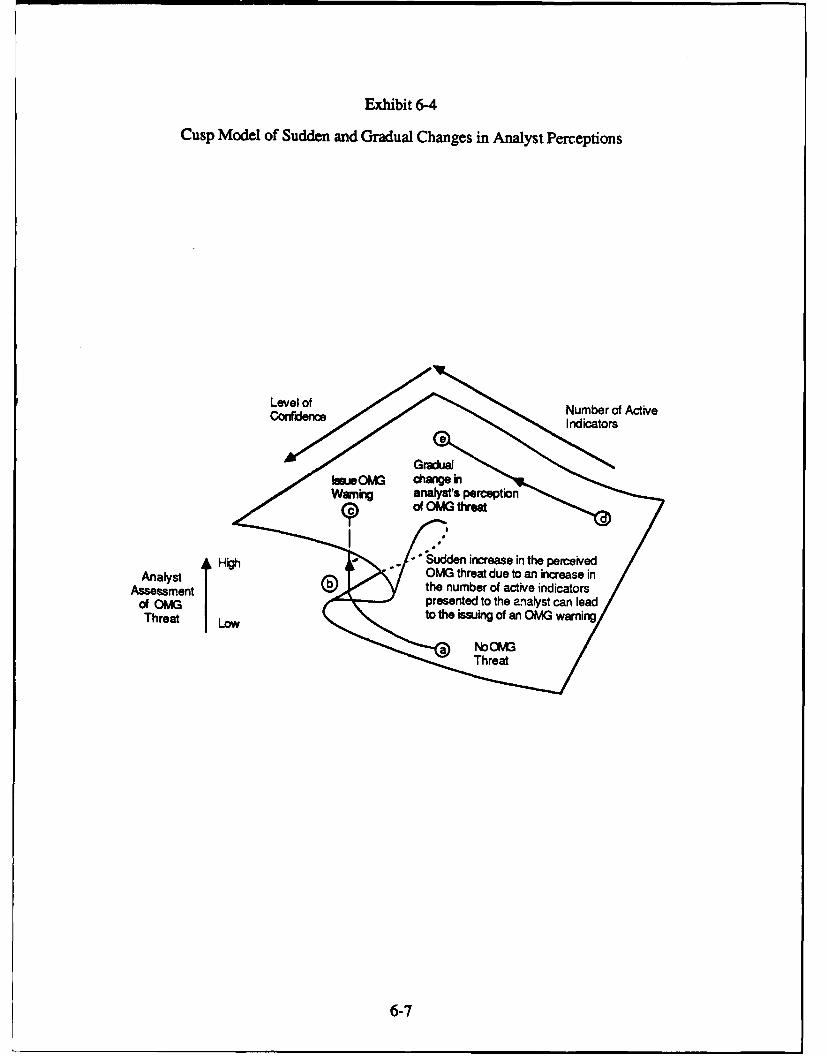
Exhibit 6-4

Cusp Model of Sudden and Gradual Changes in Analyst Perceptions

Anael te Number of ActiveConfidence Indicators

~OMG G

Warin analys's perception

of OMG threa

High Sudden increase in theAnalyst OMVG threat due to an increase inAssessment the number of active indicators

of OMGpresented to the P-nalyst can leadofea LowI to the Issuing of an OMG warnin

Threat

6-7/

Exhibit 6-5

Cusp Model of Divergent Perceptions

Level of Number ofActive

Con~mal dicaor

Divergenceno

ofIM OMG (bdcWarningarg Smalfdffrenencec

Threat Lowin perceived threat

Thret LO in erceved threat

6-8

Exhibit 6-6

Cusp Model Can Provide a New Understanding of the Causes of Perceptual Ambiguity

Level of J ' umber of Active

C4fdec Indicators

J ) Ambiguity in perception

Issu OM I caused by pre-conditioning"

. .. Warning (

Assessmentof OIVGThreat LOW

Threat

Number of Active IndicatorsLevel of

X// Region of Ambiguity

6-9

Exhibit 6-7

"Slicing" the Cusp Surface

Level of Number of Active

Numberer efnctiecatoctos

(). Fixed Numve of ACdene Indctr Va riable umber of Coienfdce evlofCofdec

Level-of

sections of the model surface have profound implications for the range of possible analystbehaviors and the nature of analyst assessments.

Thus, with a fixed number of active indicators, the "slice" of the catastrophe surfaceconsists of two apparently unconnected portions (Exhibit 6-7a) while that for fixed level ofconfidence is a continuous curve resembling an overfolded "S." Such shapes can illustrate thephenomenon of perceptual hysteresis (Exhibit 6-8), a phenomena that Woodcock has calledpartial and complete perceptual "trapping," (Exhibits 6-9 and 6-10) and counter-intuitive orparadoxical behavior (Exhibit 6-11), as described below.

6.1.6 PERCEPTUAL HYSTERESIS

Small changes in the number of active indicators (or for that matter in the level ofconfidence on the data) can lead to sudden changes in the perceived level of OMG threat andsimply returning to this initial number of active indicators will not lead to an immediaterestoration in the level of perceived threat to its existing level. This phenomena, which can beidentified as a form of "perceptual hysteresis," may be illustrated with the aid of the catastrophesurface model (Exhibit 6-8). Beginning with a low number of active indicators and low levelof perceived OMG threat, an increase in the number of active indicators presented to th,- xnalystcan lead to a sudden change in perceived threat. By contrast, beginning with large number ofactive indicators and a high OMG threat level and then decreasing the number of activeindicators can lead to conditions under which a sudden decrease in perceived OMG threat cantake place. These sudden changes in perceived OMG threat generally take place at differentnumbers of active indicators. Thus, a sudden increase in perceived threat could occur when thenumber of indicators presented to the analyst is increased from seven to eight while a decreasein threat perception might only occur when the number of active indicators is decreased fromeight to two indicators, for example.

6.1.7 PERCEPTUAL "TRAPPING"

Use of the IWCAT system by a series of intelligence analysts has led to the characteri-zation of a phenomenon which Woodcock has called "perceptual trapping." Under suchcircumstances, the analyst's perceptions would be restricted to a particular state (such as theperception of no OMG threat or the issuing of an OMG warning). The analyst would beunable to change this perception based on available data. Thus, such an analyst might continueto issue an OMG warning despite the fact that another analyst who was not similarlyperceptually trapped, would have withdrawn the warning, for example.

Exhibit 6-9 illustrates the phenomena of partial perceptual trapping while Exhibit 6-10illustrates complete trapping. Perceptual trapping occurs because an individual's perceptionsappear to be restricted to a particular portion of the catastrophe surface and no "return path"exists to permit a return to the initial state after a sudden change in perception has occurred.This restrictior is caused by the shape of the catastrophe surface and the "slices" that areconstructed from this surface. However, such a return path may be created as the result of theconsideration of an extended set of I&W indicators since the assessments of these new dataitems would lead to a change in the shape of the catastrophe model derived from these data, forexample.

6-11

Exhibit 6-8

Perceptual Hysteresis

4Decreasing number ofactive indicators

ThreatSudden increasein perceived OMGThreat Level

Increasing number of __

active indicators

Range of available Number of Active Indicators

Level of Confidence Variable fixed at its, mean value

6-12

Exhibit 6 9Partial Perceptual T-raPPing,

CK13 Da reaifg number of

Threatactive indicators

N reunPath' to low

Ragie fnadilators ~ ro ctv nd ao

Level Of Confidence Variable fixed al its mean value

6-13

Complete Percepua -Trapping,,

MGea

Derefti Numberof Active Indicators

SNo "return Path- to low0MG threat level conlditin

No retu ~ Pahtohg

Range Of avajiabl Number otive* IndiaorLevel of Confiec Varial fixed at its mean value

6-14

1. Partial Trappin g:

Partial trapping conditions occur when one type of path exists for transitions between lowand high OMG threat conditions. With the level of confidence variable fixed at its mean value,beginning with low number of active indicators and perceived OMG threat can lead to anincrease in the number of active indicators presented to the analyst and this can set the scene fora sudden increase in perceived OMG threat (Exhibit 6-9). Subsequent decreases in the numberof active indicators cannot cause a subsequent rapid decline in the perceived level of OMGthreat because no return path exists for such a transition within the limits of available number ofactive indicators supplied to the analyst. This observation, which will be substantiated belowby presenting and discussing the statistical analysis of actual analyst OMG threat assessments,reflects statements by some of the analysts that, having made a commitment to issuing an OMGwarning, a subsequent reduction in the level of information, even to a very low level, wouldnot cause these analysts to withdraw the warning.

2. Comlete Tring:

Complete perceptual trapping can occur when no path exists for a transition between thelow OMG and high OMG threat perception states (Exhibit 6-10) for a cusp surface modelconstructed on the basis of the data set presented to the analyst. Under these circumstances,the analyst's perception of OMG threat would remain at either a low or a high level throughouta complete analytic session for the complete set of number of active indicator data elements andwith the level of confidence variable fixed at its mean value, for example.

6.1.8 COUNTER-INTUITIVE OR PARADOXICAL BEHAVIOR

Cusp surface models based on analyst's perceptions of OMG threat suggest that theseperceptions may exhibit patterns of counter-intuitive or paradoxical behavior, as shown inExhibit 6-11. Beginning with a high level of perceived OMG threat and with a low number ofactive indicators and the level of confidence maintained at its mean value, a subsequent increasein the number of active indicators presented to the analyst can lead to a sudden decrease in thelevel of perceived threaL Additional increases in the number of active indicators can now causea gradual increase in the level of perceived threat, but the analyst's perceptions now appear tobe "trapped" to a part of the particular S-shaped slice of the cusp surface. Under theseconditions, a return to the initial conditions would appear to be impossible without changes inthe level of confidence or the presentation of additional sets of data elements to the analyst andthe subsequent creation of a new cusp surface model based on such an extended data set.

6.2 SPECIFIC ANALYST ASSESSMENTS

As mentioned above, several members of Synectics staff who have been involved invarious forms of I&W and intelligence analysis activity participated in testing the IWCATsystem. The following constitutes a summary discussion of the results of these different testsand the detailed analysis of these results that is presented can serve as a starting point forfurther research investigations and for the development of an operational IWCAT facility.

In each case the analyst was presented with a test data set of indicators and otherinformation described in Section 5 and asked to assess the level of OMG threat that they appearto reflected to the analyst. Following this task, the analyst was asked to designate which of theindicators were of primary importance and which were of secondary importance to them in

6-15

Exhibit 6-11

Counter-Intuitive or Paradoxical Behavior

Increasing number ofactive indicators

CM3

Sudden and paradoxical decrease in level ofperceived OMG Threat caused by an increasein the number of active indicators presentedto the analyst

Increasing or decreasing the number of active indicators causesno sudden change in level of perceived OMG Threat while movement

takes place on the *lower' part of the catastrophe surface

Number of Active Indicators

Level of Confidence fixed at its mean value

6-16

determining the level of perceived OMG threat. Information generated by this process wasthen subjected to analysis using the cusp surface analysis program.

It is a suggestive finding of the statistical analyses performed during this investigationthat the nature of the response of the different analysts to the OMG threat test data appears todepend upon their background and experience. Thus, analysts with extensive active dutytactical-level military experience (Analysts "B" and "C," below) appeared to pay almostexclusive attention to the number of active indicators, while another analyst (Analyst "D,"below) with much more national strategic-level intelligence experience appeared to pay almostexclusive attention to the patterns (or sequence type) of the displayed indicators. Analyst "A,"with extensive military and experience and involvement in more national level intelligenceanalytic activity, appeared to pay attention to both number of active indicators and their pattern.Analyst "E," with national level weapons targeting experience, performed the test and the datacollected in this process appeared to form a linear model since the cusp analysis programterminated its activities because no cubic term was detected in the analyst-derived data.

While the observation that the nature of analyst perceptions of OMG threat is predicatedby the natuxC .f the experience and training of the analysts, is a tentative finding due to thesmall sample size of analysts that were used in the experiment, such a suggestion can haveprofound implications on the way that I&W and other forms of intelligence analyses areperformed. Results of the IWCAT project suggest that analysts (who could be referred to as"front-line" analysts) closely associated with the more immediate or tactical aspects of thecombat environment concentrate on the number of active indicators while those analysts (whocould be referred to as "headquarters" analysts) who are involved in the analysis of the overallaspects of combat, and who may receive most of their intelligence input from the front-lineanalysts, appear to pay more attention to the pattern of these indicators.

If substantiated by further work and analysis, such a finding can have an importantimpact on the relationships between these front-line and headquarters analysts since the firsttype of analyst acts as a perceptual filter for the information that is presented to the second typeof analyst. The fact that these different types of analysts concentrate on different aspects of theavailable intelligence information (such as the number of active indicators or the pattern ofindicators, for example) could introduce unexpected and unintentional biases in the inter-pretation of this information and lead to a misunderstanding of the nature of particular combatsituations. The possibilities of such perceptual disconnects and their impact on I&W andcommand and control (C2) should be of concern to I&W analysts and others and furtherinvestigations with the aid of the IWCAT system would appear to be appropriate.

The following section of the report presents a description of the analysis of the I&WOMG threat data collected from five analysts who are members of Synectics staff and whohave all had experience as intelligence analysts.

6.2.1 "ANALYST A"

1. Impact of number of active primary indicators and level of confidence on OMG threatprce~tion.

Exhibit 6-12 presents the analysis of the effect of number of primary indicators and levelof confidence on OMG threat perception. The control plane plot (Exhibit 6-12a) shows that51.1% of the data are located within the bimodal zone and represent analyst assessmentconditions which are subject to ambiguity. Statistical analysis shows that a catastrophe model

6-17

Exhibit 6-12


60 CaroI Pwm plot

.. tI . .'08 0 -t-8r ("...88 MC-t

U.0 00 0 00 00 0 0 000 00 0 000 a0 S.0

1b.9 a 0 0 0 0 0 0 0 0 0 0 * 0 0 a 0 0 0 0 0 0 '..

0.0 a0 00 00 00 000 0 0a0a0 000 0 .0

3.1 0 0 a0 000 0aU00 8 0 00 a000 00 3.5

3.0 0 0 0 0 0 a 0 a 0 98 11 1 0 0 0 0 0 0 0 3.0

40 0 0 0 0 0 0 0 50 0. O 0 0 0 0 0 0 0 0 &0

3.2 0 0 0 0 0 0 0 0 0 0 a Os 0 o 0 0 0 0 0 0 * 1.0

8.0 000000 a00 0 0 0aa0 0 0 00 8.0

0.5 a 0 0 0 0 0 a 0 0 0 0 0 0 0 0 a 0 0 0 0 0 0.1

0.0 0a0 00 0 0 0 0 000 0 00 00 0 00 0.0

-0. 0 000 a00600a0 00 0 00 0c0 0 00 .0.5

-1.0 0 0 0 0 0 a 0 0 0 0 0 0 0 0 0 a 0 0 0 0 0 -1.0

81.5 0 0 0 0 a 0 a 0 0 0 0 0 0 0 0 0 0 a 0 0 0 -8.5

-0.0 00 00 0 00a0 0 000a0 0 000a00 -0.0

-0.3 0 0 0 0 0 a 0 0 0 0 0 0 0 0 0 0 0 a 0 0 a -0.3

-8.0 0 0 a 0 0 0 0 0 0 0 0 0 0 0 0 a 0 0 0 0 0 -3.0

-0 MI f. . N D. 0 8 0 3 4

~~~~~~~JJ ~~.J 9-41<i0 C aJ4Jf. oo~,8

N..0I .1 0.0 0.0. A.

0.3 *0. 0. * 0.

0.8 0. 0. 0W Thr"~'4 .

0.0 **.o .0 *. :78.9 0hr *,, 8.:.

8.12 11.280* .

8.7 0 * 8. 8.7 * 8.

-.1 0 -a.. 8.08.8.-0 C 08.0 8.0 8.

0.a * 0.0 0. * 0.

0.0 * 0* 04 .4 :0 :0.0.3 0 * 0.3 0.3 0 .5

0.0Prwpu Hy0s .0 .00 0 0.0.3pus 0 0 * 0.3 20. 0.

0. i ar *n iefr -- - - - 41o 0NN 0.3 0.0 0 0.

0.8 Vaial Prmr kxas 0od 0.8 0t 0~wec (c0.0bi "o ~rdm m Pi

0.0 0 0 .0 6 0.08

with a delay transition convention (R2 = 0.632) apears to be a more suitable model for thedata than a Maxwell convention-based model (R = 0.118), or a linear model derived with theaid of multiple regression techniques R2 = 0.464).

A slice of the cusp model surface for a range of numbers of active primary indicators andwith the level of confidence fixed at its mean value reveal situations in which partial perceptualtrapping can occur (Exhibit 6-12b). Starting with a small number of active primary indicatorsand a low level of perceived OMG threat, an increase in the number of such indicators can leadto an approximately linear increase in the level of perceived OMG threat. By contrast, startingwith a large number of active indicators and high level of OMG threat, a decrease in the numberof active indicators can lead to an approximately linear decrease in perceived OMG threat levelto a point at which a rapid decline in perceived threat can occur. Once this rapid decline hasoccurred, the analyst's perceptions appear to be "trapped" to the lower limb of the curve withno possibility of a return to the upper limb without changes in the level of confidence value, forexample.

A slice of the cusp model surface for a range of values of the level of confidence and withthe primary indicators fixed at their mean value reveal situations in which perceptual hysteresiscan occur (Exhibit 6-12c) as the level of confidence is increased or decreased. Increasing thelevel of confidence of the indicators can lead to a rapid increase in perceived OMG threat whilea decrease in level of confidence from a high to a low level can lead to a sudden decline in thelevel of perceived OMG threat. These sudden transitions in perceived threat level will generallytake place at different levels of confidence.

2. Impact of number of active secondary indicators and level of confidence on 0MGthreat percetion.

Exhibit 6-13 presents the analysis of the effect of number of secondary indicators andlevel of confidence on OMG threat perception. The control plane plot (Exhibit 6-13a) showsthat 53.3% of the data are located within the bimodal zone and represent analyst assessmentconditions which are subject to ambiuity. Statistical analysis shows that a catastrophe modelwith a delay transition convention (RI = 0.545) appears to be a more suitable model for thedata than a linear model derived with the aid of multiple regression techniques (R2 = 0.361), ora model based on the Maxwell transition convention R2 = 0.079).

A slice of the cusp surface at a fixed level of confidence and variable number of activesecondary indicators reveals situations in which perceptual trapping can occur. Increasing thenumber of these active indicators from a low to a higher level causes a gradual increase inperceived OMG threat to a condition at which a sudden change in these levels can take place(Exhibit 6-13b). Once at such a high perceived threat level, the analyst's perceptions aretrapped at this level since no return path exists for a return to lower levels without changes inthe values of the level of confidence factor. Under such circumstances, the analyst would notretract the OMG warning once issued, even with a marked decline in the number of activeindicators.

A slice of the cusp model surface for a range of values of the level of confidence and withtjie secondary incticatrs fixed at their mean value reveal situations in which perceptual hyster-esis can occur (Exhibit 6-13c) as the level of confidence is increased or decreased. Increasingthe level of confidence of the indicators can lead to a rapid increase in perceived OMG threatwhile a decrease in level of confidence from a high to a low level can lead to a sudden declinein the level of perceived OMG threat. These sudden transitions in perceived threat level willgenerally take place at different level of confidence values.

6-19

Exhibit 6-13

Analysis of 0MG Thireat Assessment Data

(14) conUrof Pla Plot

-. - *3 -. 0 0a 0 2 0 0 0 0 3

8.0 *o.0 0 0ao0o 0ooo 0 o0 0 0 2.0

0.S 0 0 a 0 0 0 a a &1 0 0 a 0 0 0 0 0 0 0 0 0 a.s

a.*0 a0@00a0 0 -Yto0 00 0 0 000 ..5 *00 0 0*0 0 0 0 a s 0 0 0 0 & ~2. a 0 0 0 a0 Is a 0 0 0 0 0 00 2.

0.5 0 0 00 0 0 00000a00 0.50.0 00 00 0 0 0 0 0 0 00 :0 0 0.0

-4.5 0 00a0 00&00 00 0 0 000 0 00 0 .5

-1.0 ** 0 **o 0 0 0 0 0 0 0 0 0 a -.

-3.3 0 0*0 0 00 0 * 0000 -*.

-0.0 00 a0 0 000 0 0000 0 0 00 00 004.0

.45 0 a 0 0 0 0 0 0 0 0 0 0 0 0 a 0 0 0 0 0 0 -4.5

0 0 0 9 *00*0a0 000a60 0 00 00 & -50

.0 0 00 0 0a00 0 00 00 00 00 0 00 0 .0

4.0 0 0 a 0 0 0 0 0 0 0 0 a 0 0 0 0 0 0 0 0 0 .0

-. 0 0 0 a 0 0 0 0 0 0 0 0 0 0 0 0 0 0 0 0 0 0 -. 0

.0 *0 00 0 00 00 0 00 0 di44ft..at0b-fq

0. 44n~~0 2 .

ftL 12 r~ 4-f I.~ E f.tw0 6.03 4-9

aft-. f a. 0.1.14 .1 t0 4".2 _I-. n2a Mkt. .1 t2

-22~ ~m~.s2~a a1.

~fl22 0. t,. S * lan.: 2*. ((.(

0921*1.4.003 22 at f ~ l 9 * n .m o n2.0 02 a)a . 442. ta.,s.Vat.

4 0 S 0 0 3- -0 -t 02.0

0..a 460, 0.0 .

2.0. 2-.0 .

a a 3.0 2.0 .

0 0.9 06.9 aO

0.0aral eoiw ae "ofCrkev C .W~ L" 0.f 0.0t ens Fie aiondr Iiat0.

0.7 * 0., 6- 0. . 0.

3. Impact of number of all active indicators and level of confidence on OMG threat

Exhibit 6-14 presents the analysis of the effect of number of all active indicators and levelof confidence on OMG threat perception. The control plane plot (Exhibit 6-14a) shows thatnone of the data are located within the bimodal zone. Statistical analysis shows that a linearmodel provides an adequate model for the data since the linear model derived with the aid ofmultiple regression techniques and catastrophe model with delay and Maxwell transitionconventions have almost equal R2 values (0.485, 0.487, and 0.487, respectively). Thisfinding is also confirmed by the data presented in Exhibits 6-14b and 6-14c, which display theeffect of variations of numbers of all active indicators and the level of confidence, respectively,on OMG threat perception.

A comparison of the material presented in Exhibits 6-12, 6-13, and 6-14 is revealing.While analysis of the data set in which impact of the primary or secondary indicators areexamined provides graphs which suggest that sudden changes in perception can take place,analyzing the effect of these indicators as a whole reveals a linear response characteristic.Under such circumstances, the combination of the responses generated by the simultaneousconsideration of the effect all the indicators can be described with the aid of a simple linearmodel. This demonstrates a major difficulty that might arise when data of different levels ofimportance to an analyst are combined for statistical or other purpose-. Such observationsshould be a matter for further consideration.

4. Impact of sequence type and level of confidence on OMG threat perception.

Exhibit 6-15 presents the analysis of the effect of sequence type and level of confidencevariables on OMG threat perception. The control plane plot (Exhibit 6-15a) shows that 41.5%of the data are located within the bimodal zone and represent analyst assessment conditionswhich are subject to ambiguity. Statistical analysis shows that a catastrophe model with a delaytransition convention (R2 = 0.472) appears to be a more suitable model for the data than aMaxwell convention-based model (R- = - 0.299), or a linear model derived with the aid ofmultiple regression techniques (R2 = 0.285).

A slice of the cusp surface at a fixed level of confidence and variable sequence typereveals situations in which perceptual trapping can occur where the analyst's OMG threatperceptions are restricted either to a high value range or a low value range (Exhibit 6-15b).

A slice of the cusp model surface for a range of values of the level of confidence and withthe sequence type fixed at its mean value reveals situations in which perceptual hysteresis canoccur (Exhibit 6-15c) as the level of confidence is increased or decreased. Increasing the levelof confidence of the indicators can lead to a rapid increase in perceived OMG threat while adecrease in level of confidence from a high to a low level can lead to a sudden decline in thelevel of perceived OMG threat. These sudden transitions in perceived threat level will generallytake place at different level of confidence values.

6-21

Exhibit 6-14

Analysis of OMG Threat Assessment Data

(a) Conf Plane Plot

4 etl q Ot t i. m

0f•0 0 0 0 00 0 aO. 0 i 0 0 0 00000 000, 00 0 a a 0 0.

0 QeW 0 a a 0.

PO.,t. sf0 ...08 ._ ,y lb O a • O •

• .o • * • o-- -- --- -- O r- - ;-- --q - .3.0 0 0 o o 0"- o 0 0 0-0 -- 0 0 a o 0 0 a .0a.o 0 -0 a0 0 -o--0- 0 0 0 • 0 * 5 0 0 8.o2.0 000a000 a0 000a0 0a0 0 0 0 058.0

*.0 0 00 0 0 0 0 0000 0 0 0 0.0

3. 00 0 0 0 000 * 00 0..0 • 0 • • 0 0 • • 0 o o oO a.0

01.0 0 a0 00 0 0 0a0Is0 0 0 0 aa0 0 00 -. 0

8.0 0 0 0 a a 0 0 0 o o 0 o 0 0 0 • • o 0 00 -0.0

02.0 0 0a0 0 0 000600 0 000 00 00 00 0.0

-1.5 0 0 0 0 0 0 0 0 0 0 0 0 0 0 0 0 0 0 0 0 0 -0.3

-. 0 0 a0 0 0 0 0 0 0 0 0 0 0 0 0 0 0 0 0 0 0 -. 0

-0. 0 0 0 0 * 0 0 0 0 0 0 0 0 a 0 0 0 0 0 0 -. S

-9.0 0 0 0 0 0 0 I0 0 0 0 0 0 0 0 0 0 0 0 0 0 -0.0

-0.• 0 0 0 0 0 0 - 0 0 00 0 0 0 0 0 0 0 0 0 0 -0.0

0 - -4 0 0 #tow

%"t W#-. Of .p, - s .

OM Thea t.", OMG Thruwmfitue

-5 - 0 0B-* •..r 0 -. .4 0 0 0 0 2

0.5 0 0 0.5 ' 0. .

Allmo Indicatorsqtl--~ll ¢e~n ,

(b) Valabli AN Inicatos.)F ) Lvatl ot CoAigo (C) tilt* UWWE, Ofml C4hc( AlIniatr

0.0 .0 0.-. . -i.6-2

.0*l A .0 0. * A * 0.0

.5 .. .. .0 ..

,.0 00 0 0....0 .0 .- 0.0

0.0 0 0 .0 0.00 0 0.0

0.o .0 ."0 0 .00., . • . 0., 0.7 . 0 0.7o,.0 0 0. 0.0 - 0.4

0.5 0 *.0 6 0.0 0 * 0.0o.0 0 .0 0 .0 0,0.

0.2 0 * 0.2 0.2 0 0 .2

0.0 * 0 * 0.8 0.0 0 0 .0

o0.1 0 • . 0.o . •0 -0.o

-.. 0 0 -.. -0.0 0 - ..

-0.0 * 0 0 -o.4 -.. 0 0 .0*.0

•-..0 0 -.. 8 -0.0 * 0 . .

-0.0 0 0 0 -0.0 -0.0 0 -0.0,-01.0- 0-0.0 -0,.0- 0 *.

-0.o - 0 0 -0.0 -0.o 0 0 0 -0.o

-0,4 * - -. 0 *|.1 * - -0.0•.0.5 * -0~ -.1 -0. - . -0.1

• l0 - -i .0 -h.t 0 -i0.0

-0l.7 - 0 "1.7 -J.7 0 -0 .7

-.. 0 0 -. 9 -I4- ...

-8.0 - 0 .4.0 -4.0 . -0.0...- " "'.0 -0.0 ie

•,• All Indicators -. 0 -. o. Lvlc ofdn 0 -.,450 -. 2 . 0l ,-0l.2

'-.0.0 ! -i.4.0 ",0.. . .

-l "4 -, 0 0 0 5 .9 -4 -l 0 I I

* e M~i ol 0lel .00em * e0

(o) Vtabl Al hIrdicators, Fbmd Lee at Confidence (c) Veribi L e at C.nfidence, Fixe AlI hcmors

6-22

Exhibit 6-15


() C~OI PWO Plot

-. -. 0 a -a 0, o 6 a a a a a .

0.0 0 a0S 0 0 0 0 0 0 0 0 0 0 0 0 0 0 0 0 0 4.

0. *O0 s ~ o e o ~ o O 0 a.. 69 9 6006 :S

0 a5 000000 0 90 7 00 0 0 0

0.0 60 a0 0 00a0 a0a0000 OO OO 0 00 0 .0

8.5 0 a0 00 00 0 040 0 00 00 0a0 006 80.

8. 0 0 00 0 0 0 070 000 0 a0 a00 08-.0

06.0 0a00 0 0000a00 0 a0 0a0 0 0 00 -0.0

-4.1 0 0 00 00 00 a0aa0 0 000 00 0 a -0.5

-2.0 0 0 0 0 0 0 0 0 0 0 0 0 0 0 0 0 0 0 0 0 0 -1.0

*8. 0 00 00 0 000 0a0 0 00 0 0 00 a -. 5

-0. 00 00 00 0 000 0 0 0 0000 0 00 -. 0

- a.0 *0 0 00 00 0 00aa0 a0 0 00 00 -. 0

-4.0 0 0 0 0 0 0 0 0 0 0 0 0 0 0 0 0 0 0 0 0 0 -4.0

0 -S -4 -1 0 0 8 9 4 5

* . "a its 6. 7 0 . 408U t o to.

4908.9- M.f 905ra1.01 a o.8888

ft I - 4998580rl 0508

90"t 0sl 916 9. 0-1 S n 8

07)8 70508 0 LI W-8 w 84. Go* I 0.48 1 4

0999N8 N,.e8 .78.508. .sst0 l ... ff o ,.0 r18q*8*t 0008 8807UI *.

-, ~ ~ ~ ~ ~ U N -

0 .6* 0.

7 .A .

*~ I.J Hystwesia s8.

30. * *0

(b .0.9w w ye.Re RWdCO W wb a* ~fbcFbdsqec y

.0.3 * .0.3 -023 *0-.

5. Impact of number of active prmary_ indicators, sequence type. and level of confidenceon OMG threat prception.

Exhibit 6-16 presents the analysis of the effect of number of active primary indicators,sequence typt" and level of confidence variables on OMG threat perception. The control planeplot (Exhibit 6-16a) shows that 54.8% of the data are located within the bimodal zone andrepresent analyst assessment conditions which are subject to ambigui €. Statistical analysisshows that a catastrophe model with a delay transition convention (R, = 0.654) appears to be amore suitable model for the data than a linear model derived with the aid of multiple regressiontechniques (R2 = 0.470), or a Maxwell transition-based cusp model (R2 = 0.315).

A slice of the cusp model surface for a range of values of the primary indicators andsequence type and level of confidence fixed at their mean values reveals situations in whichpartial perceptual trapping can occur (Exhibit 6-16b). Starting with a small number of activeprimary indicators and a low level of perceived OMG threat, an increase in the number of suchindicators can lead to an approximately linear increase in the level of perceived OMG threat.By contrast, starting with a large number of active indicators and high level of OMG threat, adecrease in the number of active indicators can lead to an approximately linear decrease inperceived OMG threat level to a point at wlich a rapid dcct le in perceived threat can occur.Once this rapid decline has occurred, the analyst's perceptions appear to be "trapped" to thelower limb of the curve with no possibility of a return to the upper limb without changes in thelevel of confidence value, for example.

A slice of the cusp surface at a fixed level of confidence and number of active primaryindicators and variable sequence type reveals situations in which perceptual trapping can occurwith the analyst's OMG threat perceptions restricted either to a high value range or a low valuerange for all ranges of sequence type values (Exhibit 6-16c).

A slice of the cusp model surface for a range of values of the level of confidenceparameter and with the numbers of primary indicators and sequence type fixed at their meanvalue reveals situations in which perceptual hysteresis can occur (Exhibit 6-16d) as the level ofconfidence is increased or decreased. Increasing the level of confidence of the indicators canlead to a rapid increase in perceived OMG threat while a decrease in level of confidence from ahigh to a low level can lead to a sudden decline in the level of perceived OMG threat. Thesesudden transitions in perceived threat level will generally take place at different levels ofconfidence.

6.2.2 "ANALYST B"

1. Impact of number of active primary indicators and level of confidence on OMG threat

Exhibit 6-17 presents the analysis of the effect of number of active primary indicators andlevel of confidence on OMG threat perception. The control plane plot (Exhibit 6-17a) showsthat 97.8% of the data are located within the bimodal zone and represent analyst assessmentconditions which are subject to ambiguity. Statistical analysis shows that a catastrophe modelwith a delay transition convention (R = 0.666) appears to be a more suitable model for thedata than a linear model derived with the aid of multiple regression techniques (R2 = 0.238), ora Maxwell transition-based cusp model (R2= - 0.339).

6-24

Exhibit 6-16

Analysis of OMG Threat Assessment Data

(a) Costr-l PlWO Plot

S.0 0 0 0 0 a b0! 00 a0 0 Swtl,. on.,l 3 i fro tl • 003 it 'qI foot..

S . - ,0 -0 0 I & a 1 0

5.0 0O000o0 v %OO0Oa- 0 O 0 00 00 0 32.0

3.3 0 a00000 6123 6I 000 131000 00 0 36.5

a.* 0 0 0 0 0 3 0 0 30 7 0 0 0 0 0 0 0 0 0 .03.0 0 0 0 0 0 0 0 0 0 0 o1 a 0 0 0 0 a 0 0 0 0 .

1.6 0 00 0 00 00003a 0000 1.0.5 0 0 0 0 0 0 00-0 000 0 00 ..

0.0 a 3 0 0 0 0 0 0 -a-- 0 , 0 0000 00 00 0.0

0.s 0 0 0 0 0 0 000000 0 a.0

1.0 00 0 0 0 0 0 0 0 0 0 0 a3.0

o0.0 000000000000000000000o • o • .•0.0

-.0. 0 0 0 0 0 a 0 0 0 0 0 0 0 0 0 0 0 a 0 0 0 .4.5

-.. 0 0 0 0 0 0 0 0 0 0 0 0 0 0 0 0 0 0 0 0 0 0 -3.0

-. 5 0 0 0 0 0 0 0 0 a 0 0 a 0 0 0 0 0 0 0 a3 0 -1.5

.4.0 0 0 0 0 0 0 0 0 0 0 0 0 0 0 0 0 00 0 0 0 -S.0

.4.0 00 00 000 ••••••••• •00000000 .00

03 - 3 34 -! 3 3 * 3

t ftOl .t 930 I S... IO".

owl., o*0003331+ III 0 " 0 0.21Z - A . l

*..o ~ ~ ~ ~ ~-b.f .11 0 S33103 fg .0 (3

0.3 * 33 * ..

:: " --:: I,

;0.2,) 0 .l-el • i 0.3 M~ I I 0. 01<.1

0. . *+ *f~ 04.0+| II eI

I.Iw Typ --- -- -- 1

Prmr kdcw 0. 0.

aid L"+.. .frd a Peld ....6-2. I.

I.o I •. 41. . I.0

I+? -• . .7 3.3I .$ • .$:3., *•" " 0.1.0 * I..

0~ .i • 00 0.3

,. * . * , .: • .o

.. •- o.. - 0..-.0 • .0.

o.. •" *" .. ..

-3.*I -0 • €. <,**•".

-. o. • * -o* -o.3-.. 0 •

•

-I.l --. *<.7

,.1.0 * 4 .14 06 -* *.0

-o. • . . -. Tye .-4.0.... o - * .- 0I',,. ..o

-,o ,* -, -,+o - -..

.4.0 * -i.0 ~.* 4.

-.3 -0** * -i.9--,

"41.0 * -.1.0 --4,

-ii.l •*-4.1* 3~

(b) Vari Pr~Tl'y Indi~t, Fbn SeUleeTypel 1V.4ii s8clU nType, Rixe Pr y lndsceto

-'l 1.L of C fec mId Lal of Conmfidence

6-25

\Exhibit 6-16 (Continued)


Lia * e3.0 16,*03.8 .tetf.a r . vl.

.3G .4 0 8

0.:,8.

a.. ~pW Hys8.0i

8.3 W 1.3iiin

id~~~~~~~~~~~~ LUal AM f Af~nFxd nkyIdc

and~~ Seu.3 Tp

Perce6-e6

Exhibit 6-17


(a) confod plwo Plot

Lst I.. Of ".. It.1 fl- . as

V . -,.1.1, *91t* Ott~l0d

0 C - - 2 - - 0 0 3 .

... 0 0 ' 000 .00 00 C O 0 0 0 0 a .

3.5 0 0 0 0 0 0 0 0 C. 0 0 C 0 0 0 0 0 0 0 3.-

3.0 0 0000 0 0 "00 0 (. 0 0 00 2,

.. 00 0 0 ...... 3 0 0 0 0 0 0.1.0- 0 0 0 0 0 0 0 0 : IC GO C 0 0 0 0 0 0 0.t

1.5 000000000 . . 0 0 00 '9.0 0 000 00 0 00000aa000,; a 0 ac a.-

0.0 00 0000 000 000 000 1.:

1C.. 0 0 0 0 0 0 0 0 0 a 0 0 0 0 0 C 0 0 0 0 0 a C.

-1.

*OO O O O O OOO-O

-0.0 0 0 0 0 0 0 0 0 0 0 0 0 0 0 0 0 0 C'.t

.5 0 0 0 . 00 0 0 0 0 C. . 0 0 0 -.

-0.0 0 0 0 a 0) 0 0 0 a 0 0 0 0 a. 0 0 0 0 0 0 0 C

- o! 0 0 0 0 0 0 0 0 0 0 0 0 0 0 0 0 0 0 0 0 -1.:

- a. 0000 C. 0 0 0 000 a0 00 0 00G0 00 -1.

-R.0 0 0 0 0 0 0, 0 0 0 0 0 0 0 0, 0 0 0 0 0. 0 0 R.!

-85 00 0 .0 0 00 0 000000000 V0 00 -&.!

-3. . o 3 *- 0 0 0 -00 0 0 0 3 0 0 5 %

0. 0 a0 0t 0 *9 t0 0d- 0 f 0a0 r0e. 0 -

oI~ a0 a 0. CR0 t~1 0 00 00 00 00

.. 0:~00 a 0.U 0 ~ t'o.-S a 00 0a 0 0 00 00 00

0l~I s.- di -t.2 fit .t. ab fy-f0. t-n

U-1tn " o -lie S 0.t. I't% 15 .* Cs-f...tU t

P-&t ti 0 O .6 . .(At Ieca ol:0V '<

0 3 -8 0. a0.3 0 0.

C MG Trous .M Threat .

I, * s. ~ I.1 * 0

*:.' *.S .

0.7~~ 0.70..

* 0.

-0. Q* .:.,-ii0

-53 * -. 3 0I S ---.. -I.. -0 .2

.00~' * 6. -0. 0.5 -a0

-0.2 . -0.2 -0.3* -.

Pwmph** Hys.3i

-3-8:0 1 3 -01 -mC.I I

(b) Vinalbh PIry h diw a Fkd Leve y Ic)t* Variable Leve of Confidanca. Fixed Prmary kidicators6-27

A slice of the cusp model surface for a range of values of the primary indicators and withthe level of confidence fixed at its mean value reveals situations in which perceptual hysteresiscan occur (Exhibit 6-17b). Starting with a small number of active primary indicators and a lowlevel of perceived OMG threat, an increase in the number of such indicatorn rqn lead to anapproximately linear increase in the level of perceived OMG threat until a threshold is reachedat which a sudden increase in threat occurs. By contrast, starting with a large number of activeindicators and high level of OMG threat, a decrease in the number of active indicators can leadto an approximately linear decrease in perceived OMG theat level to a point at which a rapiddecline in perceived threat can occur. The computed curve suggests that the analyst's percep-tion would be subject to large and sudden changes as the number of active indicators for fixedlevel of confidence values. These sudden transitions in perceived threat level will generallytake place at different levels of confidence.

A slice of the cusp surface at a fixed level of confidence and variable primary indicatorsreveals situations in which perceptual trapping can occur with the analyst's OMG threatperceptions restricted either to a high value range or a low value range for all ranges ofsequence type values (Exhibit 6-17c).

2. Impact of number of active secondary indicators and level of confidence on 0MGthreat &rceptiQn.

Exhibit 6-18 presents the analysis of the effect of number of active secondary indicatorsand level of confidence on OMG threat perception. The control plane plot (Exhibit 6-18a)shows that 72.6% of the data are located within the bimodal zone and represent analystassessment conditions which are subject to ambiguity. Statistical analysis shows that a catas-trophe model with a delay transition convention (R2 = 0.653) appears to be a more suitablemodel for the data than a Maxwell transition model (R2 = - 0.203),.or a linear mod-l derivedwith the aid of multiple regression techniques (R2 = 0.326).

A slice of the cusp surface at a fixed level of confidence and variable number of activesecondary indicators reveals situations in which perceptual trapping can occur. Starting with alow level of active indicators and low perceived threat level, the analyst's perceptions wouldremain trapped on the low OMG portion of the curve. By contrast, starting with a high level ofOMG threat and number of secondary indicators and decreasing the number of these activeindicators from a high to a lower level causes a gradual decrease in perceived OMG threat to acondition at which a sudden decline in these levels can take place (Exhibit 6-18b). Once havingachieved such a low perceived threat level, the analyst's perceptions are trapped at this levelsince no return path exists for a return to higher levels without changes in the overall level ofconfidence in the indicators, for example.

A slice of the cusp surface at a fixed level of confidence and variable number of activesecondary indicators reveals situations in which perceptual trapping can occur. Increasing thenumber of these active indicators from a low to a higher level causes a gradual increase inperceived OMG threat to a condition at which a sudden change in these levels can take place(Exhibit 6-18c). Once at such a high perr ived threat level, the analyst's perceptions aretrapped at this level since no return path exists for a return to lower levels without changes inthe values of the level of confidence factor. Under such circumstances, the analyst would notretract the OMG warning once issued, even with a marked decline in the level of confidence.

6-28

Exhibit 6-18


(a) Contol Plan Plot

-? :So o o n . ov r 3 , C o o

-4 -o -2 - I QC 0 £ 3

3.c 00 000 000 00 0 o. o..

R.0 0 o 0 0 0 0 0 0. 0 0Q a C) 0 0 09 .!

a. 0 G 3 0 0 0 0 * C, G 0 0 0 0 0 Q2.

o. 0 0 0 o 0 0 o 0 aI o o 0 0 0 o, 0 0 .

31.0 0G 00 0 o~ 00 0 0 0 C.! aao oQ

-0.t 0 0 0 0 o 0 0 0 0 0 o I0 0 * 0 0 0 0 0 0 0 .-9.4

-3.5 0 0 0 0 0 0 0 0 0 0 0 0 0 0 0 0 0 0 0 00o I ( c o ( -C.!

-. 5 o 0 0 0 0 0 0 o 0 0 o o 0 o 0 0 o 0 0() .

-5.o c 0 0 0 0 a. 0 * 0 0 a * 0 0 0 0 0 o,0 0 -.

-20 0 0 0 0 0 0 0 0 0 0 0 0 0 -.

Case0 000000000000000000000 .flow

*-a0 0 .= 0 I0 0 C 0 0 0 0 0

-00 0 0 0 0 0 0 0 0 0 00. .

-S .* 2 -E s *C* 2 4

0350r3 ft- 3 .3 f~tDob.~.

8.5 fth- 040 .tO t3ltO 0.'3

04..C351 * 0.3cf 3 ~0S 3ri *5530

* 903..*3 OC. 000 0 o. nO .3.3 30S.. CC.,* S3340fl

1.5 1 . . .

.3.0 1 . 3 :,03.

3.3 * A* .13 3.3 0 0 3.3

C., .0 od e 3.71.7C.

Z3.. fji~3 . . .

3.4*0 3. 3.40 3.

:31: Pw0j TW n 0 . 150 .C.0 0 .0 3.0 0 0 3.

3.2 4 0 3.2 .20 0.3.3 0 0 3.33.019 .

3.3r~r *rk~r 0 * Loy* o.3 5 3.33.0 4 * 3.01.1* 3.

0.9 Vam0 Sonw 0. 0.9f .ce 0ev 0.9dw a w~ Lv fCrdne ba oodr nc

0.3 . .. 0. 6-29

3. Impact of sequence tpe and level of confidence on OMG threat perception.

Data collected from this analyst for variable sequence type could not be formed into acusp model because convergence of the computational process to a particular model structuredid not take place. This result suggests that the analyst was not considering information aboutsequence type in the analysis of the OMG threat data and forming this information into a modelbased on the cusp catastrophe. The possibility that a linear or more complicated nonlinearmodel would be a more appropriate model of these data remains open.

6.2.3 "ANALYST C"

1. Impact of number of active primar, indicators and level of confidence on OMG threatrception.

Exhibit 6-19 presents the analysis of the effect of number of active primary indicators andlevel of confidence on OMG threat perception. The control plane plot (Exhibit 6-19a) showsthat 23.0% of the data are located within the bimodal zone and represent analyst assessmentconditions which are subject to ambiguity. Statistical analysis shows that a catastrophe modelwith a delay transition convention (R2 = 0.348) appears to be a somewhat more suitable modelfor the data than a linear model derived with the aid of multiple regression techniques (R2

0.295), and certainly more suitable than a Maxwell convention model (R2 = 0.145).

A slice of the cusp model surface for a range of number of active primary indicators andwith the level of confidence fixed at its mean values reveals situations in which partialperceptual trapping can occur (Exhibit 6- 19b). Starting with a small number of active pria-yindicators and a low level of perceived OMG threat, an increase in the number of suchindicators can lead to an increase in the level of perceived OMG threat without sudden changestaking place. By contrast, starting with a large number of active indicators and high level ofOMG threat, a decrease in the number of active indicators can lead to an approximately lineardecrease in perceived OMG threat level to a point at which a rapid decline in perceived threatcan occur. Once this rapid decline has occurred, the analyst's perceptions appear to be"trapped" on the lower limb of the curve with no possibility of a return to the upper limbwithout changes in the overall level of confidence in the OMG indicators, for example.

A slice of the cusp model surface for a range of values of level of confidence and thenumber of primary indicators fixed at its mean value reveals situations in which partial percep-tual trapping and paradoxical reversal in behavior can occur (Exhibit 6-19c). Starting with asmall number of active primary indicators and a low level of perceived OMG threat, an increasein the number of such indicators can lead to an increase in the level of perceived OMG threatwhich does not exhibit sudden transitions. By contrast, starting with a low level of confidencelevel and high level of OMG threat, an increase in the number of active indicators can lead to anapproximately linear decrease in perceived OMG threat level to a point at which a rapid,paradoxical, decline in perceived threat can occur. Once this rapid decline has occurred, theanalyst's perceptions would also appear to be "trapped" to the lower limb of the curve with nopossibility of a return to the upper limb without changes in the overall level of number of activeprimary indicators, for example.

6-30

Exhibit 6-19


La~0~ C'. t. 02 g.tO 0 t.

a 0t 0. 0 0 33 Ct02 0 9 t~l 0 '.tter00 0 . -

-.0 0 -2 .3 0 0 0 0 0 0 0 a 0 0 5 .

2.0 0 0 0 0 a 0 0 0 0 0 0 C. 0 0 0 0 0~ C 0 0 0 3.!

3. 00 0 0 00 00a0 C. r' 0 000 0000 0 .!

11.0 0 0 0, 0 0 0 0 0 0 0 0 0 0 0 0 0 0 a a 0 0 a .

2.z 0 00 0 0 00 0 00&0 00 0 000 00 0

2.0 0 0 0 0 0 01 0 0 0 03 0 0 0 0 0 0 0 0 0 0 0

3.t 0 0 . 0 0 00 00000 a0 (.0a00 a0 00 0.

3.0 0 000 a0 00 0 0-a00 00a0 0 000 0.

o. a 00.00000a01 C.9 00 00 00 00a0 0 I(.!

0. 0 000a0 00a0 0&500 00a00 000 0 -. '

0. a 0 0 a 0 0 0 0 0 0) 0 0 0 0 0 0 0 0 0 0 01.!

(A.0 0 0 0 0 0 0 0 0 0 03a 0 0 0 0 0 0 0 0 0 0 01.

-0.0 0 0a 0 0 0 0 0 0 0 0 0 C 0 0 0 0 0 0 0 -2.

-3.( 0 0 0 0 0 0 0 0 0 030 0 0 0 0 0 0 0 0 0 0 -7..!

-1.C. 0 0 00 00 0 0000a0 00 a0 00 00 0

-. 5 0 0 0 0 0 0 0 0 0 0 0 a 0 0 0 0 0 0 0 0. 0 -0

3.5 . 0 0 0 0 0 0 0 0 0 0 0 0 0 0 0 0 0 0 0 0 0 -5.!

-0 et 0 t 0 F 0 n 0 h 0 fa 0 0 0 0 0 00 0 -.

4.. 0 0 0 30 0 0 0 0 0 0 0 0 t

-3 -4 -2 04 1 00

09.S ttth t . tg.3

L3*... ~ ~ ~ ~ I. it: 2 .9 I~113 *03?

Pereie 43* .03 ttt.tq.i.. 0.v.tff

3.0 0 0.1. 3.0 .

3:.* 3. . ..

*~~~ ~ 0 . . .

'0: I. ...*

*0 3 o.- i,

* 0. 0 .90 9 k 0 .

0..10 3 * (

0 0.! 0.5

* ~0.3 0.2 2

* 0.& - 00 '.

0 .4. -o

6.5 -3.21. 3

2. Irpact of number of active secondary indicators and level of confidence on OMGthreat c in.

Exhibit 6-20 presents the analysis of the effect of number of active secondary indicatorsand level of confidence on OMG threat perception. The control plane plot (Exhibit 6-20a)shows that 26.7% of the data are located within the bimodal zone and represent analystassessment conditions which are subject to ambiguity. Statistical analysis shows that acatastrophe model with a delay transition convention (R2 = 0.489) appears to be a moresuitable model for the data than a linear model derived with the aid of multiple regressiontechniques (R2 = 0.392), and certainly more suitable than a Maxwell convention model (R2

-

0.099).

A slice of the cusp surface at a fixed level of confidence and variable number of activesecondary indicators reveals situations in which perceptual trapping can occur. Increasing thenumber of these active indicators from a low to a higher level causes a gradual and approxi-mately linear increase in perceived OMG threat to high level (Exhibit 6-20b). By contrast,starting with a large number of secondary indicators and consequential moderate level ofperceived OMG threat, reducing the number of these indicators can lead to conditions underwhich a rapid increase in the level of perceived threat can occur.

A slice of the cusp model surface for a range of values of the level of confidence and withthe secondary indicators fixed at their mean value reveals situations in which perceptual hyster-esis can occur (Exhibit 6-20c) as the level of confidence is increased or decreased. Increasingthe level of confidence of the indicators can lead to a rapid increase in perceived OMG threatwhile a decrease in level of confidence from a high to a low level can lead to a sudden declinein the level of perceived OMG threat. These sudden transitions in perceived threat level willoccur at different level of confidence values.

3. !mpact of'number of all active indicators and level of confidence on OMG threatperception.

Exhibit 6-21 presents the analysis of the effect of the number of all active indicators andlevel of confidence on OMG threat perception. This actual data was the first collected from anyanalyst during the IWCAT pre-testing and was performed before the concept of primary andsecondary indications was established. This development took place during the "Analyst C"test session and the complete set of indicators was subsequently broken down into thesecomponents after discussions with the analyst concerned. The control plane plot (Exhibit6-21a) shows that 3 1.1% of the data are located within the bimodal zone and represent analystassessment conditions which are subject to ambiguity. Statistical analysis shows that a catas-trophe model with a delay transition convention (R2 = 0.570) appears to be a more suitablemodel for the data than a linear model derived with the aid of multiple regression techniques(R2 = 0.414), and certainly more suitable than a Maxwell convention model (R2 = 0.125).

A slice of the cusp surface at a fixed level of confidence and variable number of activeindicators re'eals situations in which perceptual trapping can occur. Increasing the number ofthese active indicators from a low to a higher level causes a gradual and approximately linearincrease in perceived OMG threat to high level (Exhibit 6-21b). By contrast, starting with alarge number of active indicators and consequential moderate level of perceived OMG threat

6-32

Exhibit 6-20


is) Canw~ Pwoj po

....... *.C W33.,0303339f300

5?.0 0 r, 0 0a 0onr a143 0 00.,0 0 S

-0 a 0 0- a 0 0 £ . 0 0

. 0 0 0 00 0 00 0 000a0 00

0 00 00 a00*0 0 a0 000 0 00 0a 3..!

3.0 0 0 00a0 000a000 00 (0 00 00 00

3. a 00000 00 03010 00 aa0 000 1.:

3.0 0 00000a0aa00 31a0 00 0000 0C.

1.5 0 0a0 0 0 00 00017 00 0 a000 c 3>

1.0 0p0 000a00a 0 q9 ae co 0 0 a0 1.

0.50 00 0 000a000400 a0 000 0 C.

0.0 0 0 0 0 0 0 0 0 0 0 a 3 0 0 a 0 0 0 0 ..

-05 a 0 0 0 a 0 0 0 0 7 a a a 0 0 0 0 0 0 0 .. !

-30 0 0 0 0 0 0 0 0 a 0 1 & 7 0 0 0 0 a a 0 0 -1.

-3.5 0 0 0 0 0 0 0 0 0 0 a A 9 0 0 0 0 0 0 0 0 C1..

-1.0 0 a 0 0 0 0 0 0 0 0 0 0 3 0 0 a 0 0 0 0 0 -E.

-3.5 0 0 0 0 0 0 0 0 0 0 0 0 0 0 0 a 0 0 0 0 0 -&3!

-2.0 00 a00 0 0000a0 00 0 00 0a000 -1.

-. 0 0 0 0 0 0 0 0 0 0 0 0 0 a 0 0 0 0 0 0' 0 0 -.

.5 00 00a0 00 00 0 00 0 0 00a000 -A.,

-0.0 0 0 0 0a00 00000 00a00a0a0 00 -S.

-5 d 4 ~ A. -h sb- 0 3 3 3

Lino, M0 2 0.292 3nt3tpa 'W"....noo

.=!.3 3 0.0"9C33k3. mon

.t.f.O Saf In3. 0w .37 -<(c<

affWo f .11"1 30 3.hodF &.5. sC0000.00.3 t t-C 0.330 l(nfl of o.r&. I* P. NoC@3Q all &L,-. c.,.t.-ta to.,nn.3..

3.0~~ : 0 ,3 *

3.0. . 0 3.0 0.8** 03.1t 0hm 0 .3 3

3,.

6330

Exhibit 6-21


(a) Contal PWMi Plot

L..t.on of Said in 040 0 3.I uoco.

0rhn~a 54 a ytr 5a~ 0 0 0 0

3.0 0 00 0 0 0 0 0 0 0 0 0 0 0 0 0 0 0 0 .

0.5 0 0 0 0 0 0 0 0 a A 0I a a a 0 0 0 0 0 2.!

0.0 0 00 0 0 0 00 00000!-a0 000

. 0 0 000 0 00 1 .0a 0 00 02.

. 0 0 0 0 0 0 0 0 0 It a 0 0 0 0 0 0 0 0 1.(

1.5 0 0 0 0 0 0a 0 0 1 6 0 0 0 0 0 0 0 0 0 1.!

0a 000 0 000 0202 0 00 00 00 00I.5

0.5 00000 a 00 000a00 00 t,.!

0.0 0 0a0 0 00a00 0 6 00 00 00000 a.

-0.5 0 0 000 a0a0 0 2vA.9000 00000 0

-0.% 0 0 0 0 0 0 0 0 a 0 0 0 0 0 0 0 0 a 0 -1.!

-a.0 0 0 0 0 0 0 0 0 0 0 0 0 0 0 0 0 0 0 0 -ff.I

-1.5 000 0 00 000a0 200 0a0 00 00 -2. T

-0.0 0 0 00 0 0a0 000 040 00 00 0 00 -S.,

-3.5 0 0 0 0 0 0 0 0 0 0a 0 0 0 0 a 0 a 0 0 0 -7.!

-. 0 0 0 0 0 0 0 0 0 0 0 0 0 0 0 0 0 0 0 0 0 0 -. ,

-2.% 0 00a000 a00a00a00a00 00a0 00 -. T

-5.0 0 0 0 0 0 0 0 0 0 0 0 0 0 0 0 0 0 0 0 0 0 -S. c

L a n d P - 4 , 4 I 0 2

f0 $MOI -M. -1Wt e0- Wo tw. tt.t -ofl.LS 1 R 0.2 3Il 95t

0.0 *0.5 .5 *0.2

0. a .. 0* 100. 0.2 0.2 * 0.23

0.0 * 00 .9 0.00.1 *0.1Pris 0.5

.0 * 0 0 0 0 .05.9 * 1.4 .3

-0 I0& Ln w o-:S. MTs ~

A 5.7W

I.. a 5.40 .~%

4b) Vo 1.1 M. *f -,1. oe o M2 wWdCrdm Fo Dko

5.0 * 5.0 506-34.

and reducing the number of these indicators can lead to conditions under which a rapid increasein the level of perceived threat can occur.

A slice of the cusp surface at a fixed level of confidence and variable number of activeindicators also reveals situations in which perceptual trapping can occur. Increasing thenumber of these active indicators from a low to a higher level causes a gradual increase inperceived OMG threat to a condition at which a sudden change in these levels can take place(Exhibit 6-21c). Once at such a high perceived threat level, the analyst's perceptions aretrapped at this level since no return path exists for a return to lower levels without changes inthe overall number of active indicators. Under such circumstances, the analyst would notretract the OMG warning once issued, even with a marked decline in the level of confidencce inthe active indicators, for example.


Data collected from this analyst for sequence type variation could not be formed into acusp model because convergence of the computational process to a particular model structuredid not take place. This result suggests that the analyst was not considering information aboutsequence type in the analysis of the OMG threat data and forming this information into a modelbased on the cusp catastrophe. The possibility that a linear or more complicated nonlinearmodel would be a more appropriate model of these data remains open.

6.2.4 "ANALYST D"

1. Impact of number of primary. secondary. and all active indicators and level ofconfidence on OMG threat perception.

Data collected from this analyst for primary, secondary, and all active indicators andanalyzed separately could not be formed into a cusp model because convergence of the com-putational process to a particular model structure did not take place. However, a model couldbe formed from sequence type and level of confidence data produced by this analyst (seebelow). This result suggests that the analyst was not considering information about thenumber of active indicators, l -s, in the analysis of the OMG threat data, or that another typeof model (such as some form of linear model, or much more complicated nonlinear model) ofthese data was more appropriate.


Exhibit 6-22 presents the analysis of the effect of sequence type and level of confidenceon OMG threat perception. The control plane plot (Exhibit 6-22a) shows that 74.1% of thedata are located within the bimodal zone and represent analyst assessment conditions which aresubject to ambiguity. Statistical analysis shows that a catastrophe model with a delay transitionconvention (R2 = 0.606) appears to be a more suitable model for the data than a linear modelderived with the aid of multiple regression techniques (R2 = 0.097), or a Maxwell transition-based cusp model (R2 = - 0.740).

6-35

Exhibit 6-22

Analysis of 0MG Threat Assessment DataOR) Coi*cI Pwmg i

..3.~a .. ,l.c~,. 3.333- y D~~

%..0 0 0a0 0 0 0000 .0a0 0a00000 C. t

CS 0 0 0 0 0 C 0 0 0 0 0 0 0 0 0 0 0 0 0 0 0

2.5 0 0 0 00 00 00 0400 00aa000 .0 .

1.0 0 01 0 0 0 0 0 0 0) C, 13 0 (. 0 0 0 0 0 0 c 0

&.5 0 0 c 0 a 0 0 0 c 0 It 0 0 0 0 0 0 0 0 V' 0 L.'

2.0 0 0 0 0 0 0 0 0 0 0. Is 0 0. 0 0 0 0 0a . 0

A.S 00 a00a0 000 02 U 0 00 00000 3.

1.0 0 000 0 00 00 aCto 0 00 0 000 C. C 3.

0.A 0 000000V0 0393IF: 0a0 0 00 0 000 C.

0.0 0 0.0 0 0 00 003:0 00 00 0 0 000 0,C

-13.(- 0 0 0 0 0 0 0 0 0 7 0 0 a 0 0 0 0 0 0 c' 0 -1.

.35 0 0 0 0 c 0 0 0 (' a 0 0 0 0 0 0 0 a 0 0 C.

.0 0 0 0 0 0 0 a0 C 0 0 0 0 0 0 0 0 0 0 0' 0 C r

-. 5.0 0 00 a00a0 000 coo 00 0,0 0(.DC. -E.:

-3.0 0 0 0 0 0 0 0 0 0 0 0 0 0 0 0 0 0 0 0 0 0 -3.

-. 0 0 C0 c 0 0 0 0 0 0 0 0 0 0 0 0 0 0 0 0 00 -.

-50 0 0 0 0 0 0 0 0 0, 0 0 0 0 0 0 0 0 0 0 0 a

-s - a -. 0 -l0 0 3 0 0 0 1

0~a - V - ft i n *f.t figur.

tin.., ~ ~ ~ ~ -it A. .9 gt133 9

M,): Or-tae Of Cas in b3... 2v-0 0.793 -44<<%

. *-3 0 a 3 ~-

2.. . . 9.. 9.9 a . .0

Peosve 1. .: . I. .1.3 OM T3 .3 S 1:.

2.0~ OM 1hred*902. P~3fl'(

'a19.. 3.9 .9 * C 3.

0.':0' 37 a 3

C.3 *0: .3 la . .

* .0 .0* .01

0 0.0. .

0.7 C 9 --0.7 0. . 0.

0.9 . 9 0 -0 O. I .

0 1 -0.1 4.-0.1 * .! -0. 1 0.

- ~ * -02, 0.2 C. 0.

* o~v Typ 3. 1 LOV.1 d C49

-0.5 * ~0.5 -031 -.

0.9 w~I S~= ye *ba 9aY of Co..w 6-06 ao -0.9LW mlrm idS eT

A slice of the cusp surface at a fixed level of confidence and variable sequence typereveals situations in which partial perceptual trapping can occur. Increasing the sequence typeparameter from a low to a higher level causes a gradual and approximately linear decrease inperceived OMG threat (Exhibit 6-22b). By contrast, starting with a large sequence parametervalue and a high level of perceived OMG threat and reducing this parameter can lead to con-ditions under which a rapid decrease in the level of perceived threat can occur and whereperceptual trapping can take place.

A slice of the cusp surface at a variable level of confidence and fixed sequence parameterreveals situations in which partial perceptual trapping can occur. Increasing the level of confi-dence from a low to a higher level causes almost no change in perceived OMG threat to highlevel (Exhibit 6-22c). By contrast, starting with a large level of confidence and high level ofperceived OMG threat and reducing the level of confidence of the I&W input data can lead toconditions under which a rapid increase in the level of perceived threat and perceptual trappingcan occur.

6.2.5 "ANALYST E"

Despite collecting a complete data set from this analyst, computer analysis of the datarevealed that these data would be best fitted by a linear model. Indeed, the statistical analysiswas terminated because of the low level of the cubic term in the analysis or the nonlinear natureof the data itself.

6-37

APPENDIX A: AN OVERVIEW OF CATASTROPHE THEORY

Catastrophe theory and related mathematical modeling techniques can illustrate the impactof command and control on military behavior and be used to support the activities of I&Wanalysts. They can also provide new methods to support the military decision-making processthat can exploit intelligence and other types of data. Models developed by Woodcock (1986)and based on the theory describe the impact of command and control, firepower, and forcestrength on military force survivability. Other mathematical models developed by Woodcock(1986) describe spatial and temporal oscillations in military force strength and the emergence ofchaotic behavior under appropriate conditions.

Catastrophe theory provides a rigorous mathematical framework to support the "top-down" analysis of complicated military systems in general, and the high level managementpolicy- and decision-making activities of military planners and others in the command andcontrol and indications and warnings arena, in particular. The theory can be used to analyzethose systems in which gradually changing forces can give rise to either gradual or suddenchanges in beha';ior in, the same system under different conditions. This behavior can bedescribed with the aic! of specialized catastrophe diagrams that capture the essence of systembehavior by expressing the causal relationships between the input variables (known as controlor conflicting variables) and output variables (known as behavior variables).

Catastrophe theory can be used to analyze those systems which exhibit at least some ofthe properties of hysteresis, bimodality, and divergence. The theory is particularly usefuluider those circumstances in which gradually changing forces can give rise to either gradual orsudden changes in behavior in the same system under different conditions. It is also usefulunder conditions involving ambiguity and uncertainty such as those faced by I&W analysts.

A. 1 CATASTROPHE THEORY - A PROVEN FRAMEWORK

Invented by Thom in the 1960's (Thom, 1969, 1975; Brocker and Lander, 1975; Postonand Stewart, 1978; Zeeman, 1977; Zeeman and Trotman, 1977; Woodcock and Poston, 1974),the theory has been used in many applications in the mathematical, physical, life, and socialsciences (see Arnold, 1984; Berry, 1976; Cobb, 1978; Gilmore, 1981; Hilton, 1978; Janich,1974; Lu, 1980; Stewart, 1981; Stewart and Peregoy, 1982; Stewart and Woodcock, 1981,1984; Wilson, 1981; Woodcock, 1978, 1979; and Woodcock and Davis, 1978; for example).Catastrophe theory has also been used in a series of military applications by Woodcock, 1986;Woodcock and Dockery, 1984 a, b; 1986 a, b; Dockery and Chiatti, 1986; Dockery andWoodcock, 1986 a, b; Isnard and Zeeman, 1976; and Holt, Job, and Marcus, 1978; and tomodel the phenomenon of bistable and multistable perception by Poston and Stewart (1978b)and Stewart and Peregoy (1982).

Thom called sudden changes in behavior "catastrophes" and developed a theory (subse-quently referred to as "catastrophe theory" by Zeeman) as a new method for analyzing andclassifying these changes. The elementary catastrophes are the simplest distinct patterns ofchanges that can occur in many types of systems. There are seven distinct elementary catas-trophe manifolds. These manifolds are geometric surfaces that are generated from combina-tions of the stationary state points of systems with up to four input variables (referred to ascontrol factors) and two output variables (referred to as behavior variables).

A-1

The elementary catastrophe manifolds have a complexity ranging from thetwo-dimensional fold catastrophe (with one control factor and one behavior variable) to thesix-dimensional parabolic umbilic catastrophe (with four control factors and two behaviorvariables). Mathematical details of these catastrophes are summarized in Exhibit A- 1. Thepopular names presented in Exhibit A- I are descriptive of the geometry of their catastrophemanifolds as shown in Woodcock and Poston(1974) for example.

Exhibit A- 1

The Elementary CatastrophesIControl Behavior

Popular Name Factors or Output Potential Function Equationof Catastrophe or Input Variables

Variables

Fold 1 1 x3/3 + ax

Cusp 2 1 x4/4 + ax 2/2 + bx

Swallowtail 3 1 x5/5 + ax3/3 + bx 2/2

Butterfly 4 1 x6/6 + ax4/4 + bx 3/3 + cx 2/2 + dx

Hyperbolic Umbilic 3 2 x3 + y3+ wxy + ux + vy

Elliptic Umbilic 3 2 x3 - 3xy 2 + w(x2 + y2 ) + ux + vy

Parabolic Umbilic 4 2 x2 y + y4 + ty2 + wx2 + ux + vy

where (a, b, c, d, u, v, w, and t are control factors and x and y are behavior variables).

In applications in which the elementary catastrophes are used, an attempt is made todevise the simplest possible model (that is a model which uses as few control factors andbehavior variables as possible) that can capture the essence of system behavior. Once thenumber of dependent and independent variables at work in a particular system has beenidentified, elementary catastrophe theory provides an indication of which of the catastrophemanifold diagrams is appropriate for expressing the causal relationships between thesevariables. Such diagrams can provide a basis for undertaking a series of "thought-experiments" in order to determine the response of the system to changes in the magnitude ofthe controls to which it is subjected.

Thom's theorem claims that the stationary state behavior of all systems (includingphysical, chemical, biological, and societal systems) with up to four control factors (or inputvaiiab1c ), two 1iavior variables (or outputs), and which possess an associated potentialfunction can be described with the aid of one of the elementary catastrophes. Subsequentmathematical analysis by Zeeman and Trotman (1977), for example, has proved Thom'stheorem.

A-2

The use of catastrophe theory to model a particular system, such as that associated withmilitary combat, will require the identification of a suitable set of control factors and behaviorvariables. Two and four control factor models of military behavior, which are based on thecusp and butterfly catastrophes respectively, have been developed by Woodcock and Dockery(1984 a, b). The development of these models was motivated, in part, by the need to providemodels with relatively few control factors that resemble the properties or "axes" around whicha battle commander organizes his perceptions.

Following this work, Dockery and Chiatti (1986) have used a statistical programdeveloped by Cobb (1983) to fit simulated combat data to the surface of the cusp catastrophemanifold. Such models can provide a useful type of interface between the military commanderand elaborate computer-based combat simulations which provide large amounts of data. Thesemodels can provide a series of diagrams, which can be referred to as "problem-solvinglandscapes," that can aid the commander in tracking events during combat and support histactical and strategic decision-making processes by enabling him to perform a series of situationassessments and impact analyses on an essentially real time basis.

While elaborate simulations can provide considerable insight into the nature of the combatprocess, the complexity and magnitude of the data that they produce serves to reduce theirutility as a guide for the military commander. By contrast, the catastrophe models provide amethod for presenting information in a method which can aid comprehension and "turn oldfacts into new knowledge" (Thompson, 1917).

A.2 THE PROPERTIES OF THE CUSP CATASTROPHE

The properties of the elementary catastrophes can be illustrated by the cusp catastrophe.The cusp catastophe potential function (Vcc(x)) is the sum of the germ (gcc(x)) andunfolding (ucc(x)) components of the catastrophe, that is: &

VCC(x) = gCC(x) + ucc(x) = x4 /4 + ax2/2 + bx (Al)

where a and b are the control factors, x is the behavior variable, and gCC(x) and ucc(x) are thegerm and unfolding of the catastrophe, respectively. The properties of equation (A1) areillustrated in Exhibit A-2 for various values of the a and b control factors.

Conditions in which both a and b in equation (Al) are zero describe the germ of thecatastrophe (Exhibit A-2). Nonzero control factor values represent conditions in which thegerm is perturbed or unfolded and the effect of such control factor changes reveals theunderlying structure of the germ of the catastrophe.

Stationary states of the cusp catastrophe potential function (equation (A1)) occur when itsdifferential with respect to the behavioral variable (x), vanishes, that is, when:

dVCC(x)/dx = x3 + ax + b = 0 (A2)

This equation describes a three-dimensional (x, a, b) curved surface known as the catastrophemanild which represents the stationary states of the function (A2) as shown in Exhibit A-3.The catastrophe manifold equation has either one or three real solutions depending on thevalues of the a and b control factors. The single solution is a minimum while the triple solutionrepresents two separate minima separated by a maximum. Equation (A3), representing thebiLurai.on set (that is, the set of control factor values at which one or other of the minima is

A-3

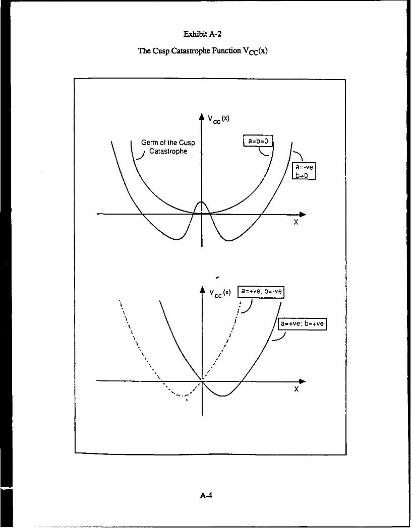
Exhibit A-2

The Cusp Catastrophe Function VCC(x)

AVcc(x)

Germ of the Cusp bo~Catastrophe -

VCC(x) la+e~b=vel

''a-

Exhibit A-3

The Cusp Catastrophe Manifold and Control Plane

Sude ang Gua Catatrph

on rea Behavior

bb

Bifurcattopoe Set

(4a 3+ 27b 2=0) three realsolutions

Control Plane

x 4 ax2+bCC(X) + 2 b

A-5

destroyed in response to system changes), can be obtained from the cusp function (1) by

differentiation and rearrangement

4a3 + 27b2 = 0 (A3)

Sudden or catastrophic transitions of state can occur in response to changes in controlfactor values at the bifurcation set as one of the two minima of the catastrophe function (A2)disappears and becomes a point of inflection. Non-catastrophic changes in behavior can occurwhen changes in control factor values do not cause a change in the number of stationary statesof the catastrophe function.

Both types of changes in system behavior can be illustrated by the pattern of movementof a point, known as the statep2ini on the catastrophe manifold surface in response to changesin control factor values. Thus, path (p, q, r) (Exhibit A-3) represents a sudden or catastrophicchange in system behavior while path (s, t, u) represents a gradual change in system behavior.

A.3 THE PROPERTIES OF THE BUTIERFLY CATASTROPHE

The butterfly catastrophe function (VBC(x)) has the form:

VBC(x) = x6/6 + ax4/4 + bx3/3 + cx2 /2 + dx (A4)

which represents a potential function with at most three stable stationary states separated bytwo unstable stationary states for particular values of the control factors (Exhibit A-4a). Thethird stable stationary state can be considered as an intermediate or compromise state betweentwo polarized extreme states. It is represented by an additional, intermediate layer of the butter-fly catastrophe manifold surface (Exhibit A-4b). This exhibit is a three-dimensional projectionof the five-dimensional manifold drawn with the a and b control dimensions fixed in value.Other projections look similar to the cusp manifold (see Exhibit A-3, for example) except thatthe f.ldrdregion of the butterfly manifold can move back and forth. In the four factor modelof military behavior described below, this intermediate layer represents a state of intermediateBlue force survivability which is supported by appropriate levels of Blue force firepower andcommand and control capabilities.

A.4 CATASTROPHE THEORY-BASED MODELSOF MILITARY BEHAVIOR

The following is a description of two models of military behavior based on catastrophe

theory that has been developed by Woodcock and Dockery (1984 a, b; 1986 a).

A.4.1 A CUSP-CATASTROPHE-BASED MODEL

The first catastrophe-theory model of the combat process developed by Woodcock andDockery (1984 a, b) describes the impact of opposing Red and Blue forces on the survivabilityof the Blue forces. This model involves the impact of two influences on system behavior and.as a consequence of Thom's ticorern, is based ca, hczusp a;ai.ophc.

A-6

Exhibit A-4

The Butterfly Catastrophe Potential Function VBc(x) and Manifold

ControlCotl

BehaviorVariables (x)

(b)5

The Butterfly Catastrophe can represent systems with up to three stable stationary statesand two u~iabie stationary states and whose behavior is determined by the impact 3ffolir key influenf-s (or control factors).

V BC (x) =x/6 +ax 4 +bx3/3+ cx 2 2 + d

A-7

The concept of using conflicting factors (which is due to Zeeman (Isnard and Zeeman,1976)) in place of control factors was employed by Woodcock and Dockery (1984 a, b; 1986a) in both the two factor and four factor models in order to capture the inherently conflictualnature of the military combat process (Exhibit A-5). Two areas of the cusp catastrophe mani-fold, which represent two qualitatively different types of system behavior, can be identified. Acondition of high Blue and Red Force strengths is represented by a point at position (a) on thecatastrophe manifold surface. As the combat proceeds, a relatively large degradation of theBlue Force strength compared to that of the Red Forces can lead to a rapid decrease in BlueForce survivability path (a-b-c).

This two factor model has illustrated the impact of Blue and Red force strength on thesurvivability of the Blue forces. Together with the fitting of simulated data with a programdeveloped by Cobb (1983), and by Dockery and Chiatti (1986), one result of which is illus-trated in Exhibit A-6, this model has provided an anchor for further investigations. The line ofreasoning takes quite literally the concept that lower dimensional manifolds are embedded inthose of higher dimensions.

A.4.2 A BUTTERFLY-CATASTROPHE-BASED MODEL

The second model describes the impact of Red and Blue force strength, firepower, andcommand and control capabilities on the survivability of the Blue forces and is based on thebutterfly catastrophe (Exhibit A-7). The relative firepower and command and control capa-bilities available to the two forces will be represented by scales which will be placed below thedrawing of the three-dimensional section of the five-dimensional butterfly catastrophe mani-fold. As the position of the indicator arrow moves on the scale, the shape of the manifoldchanges. We track these changes by comparing the changes in the shape of the "footprint" ofthe folded region of the manifold.

The conditions in which the Blue force has a significant advantage in firepower andcommand and control capabilities compared to the Red force, is illustrated in the model by adistortion of the manifold surface to produce a relatively large region. This is identified withconditions of high Blue force survivability. These additional influences can thus be seen tooffset the effect of a relatively low intrinsic Blue Force strength.

A reduction in the Blue force command and control capability advantage during combatwill lead to a reduction in Blue force survivability. Under these circumstances, it wouldperhaps appear to the Blue Force Commander that the "ground" was falling away from underhis feet as the folded region of the surface moves in response to changes in the level ofcommand and control capabilities (path a-b, Exhibit A-7) in response to a decrease in the levelof Blue force command and control capabilities. The hatched area drawn on the plane in thisExhibit represents those sets of factor values for which such a reduction in force survivabilitycan occur.

A-8

Exhibit A-5

A Military Analysis and Problem-Solving Landscape

Blue ForceStrength

aBlue Forcet opSurvivability Sudden

Reduction inFBlue Force

Gb SurvivabilityReFoc

Strength

•A two factor catastrophe model

-force balance determines force survivability

A-9

Exhibit A-6

Application of Catastrophe Theory to Military Analysis

Number of

AttackersRegionCatastrophe Regl

Stockpile

120 COMO IIIReplicatilons

(Re-drawn and modified, after Dockery and Chiatti, 1986)

Control plane plot of 120 replications of the second scenario taken from the event drivensimulation. The independent variables are stockpile (XI) and number of attackers (X2).

Values of XI, X2 used were total over several time periods.

A-10

Exhibit A-7

A Military Analysis and Problem-Solving Landscape

Blue ForceStrength

7/ "'"

Blu BleooreredFoc

Forceiurvivbilit

etorci ioBlue Force ndFSuControllCap arenlti

,,"~~ / to in Blue.Rdutono" ( lue Frce Re Forc

""" ""orc Survivability Srnt

due to reduction inJ Command and

I Control Capabilities

Firepower

Command and Control

Force balance, firepower, and command and control capabilities determine force survivability.

A-1I

BIBLIOGRAPHY

Arnold, V. L, Catastrophe Theory (Translated by R. K. Thomas). Berlin and NewYork: Springer-Verlag, 1984.

Berry, M. V., "Waves and Thorn's Theorem." Adv. Phys., 1976, 25, 1-26.

Bonder, S. and J. G. Honig. "An Analytical Model of Ground Combat: Design andApplication." Proceedings of the Tenth Annual U.S. Army Operations ResearchSympsium. Durham, North Carolina, 197 1.

Brocker, T. and L. Lander. "Differential Germs and Catastrophes." LondonMathematical Society Lecture Notes, 17, 1975, Cambridge: Cambridge UniversityPress.

Cobb, L. "Stochastic Catastrophe Models and Multimodal Distributions." BehavioralS 1978, 23, 360-374.

Cobb, L. "Estimation Theory for the Cusp Catastrophe Theory Model." Proceedings ofthe Section on Survey Research. Washington, DC: American Statistical Association,1980.

Cobb, L. A Maximum Likelihood Computer Program to Fit a Statistical CuspHypQthesis. The Hague, The Netherlands: SHAPE Technical Centre, 1983.

Cobb, L. and G. Harrison. A Computer Program to Solve Stochastic LanchesterEuations. Washington, DC: Organization of the Joint Chiefs of Staff, 1985.

Dick, C. J. "Soviet Operational Maneuver Groups: A Closer Look." InternationalDefense Review. 769-772, 1983.

Dockery, J. T., and L. Chiatti. "Application of Catastrophe Theory to the Problems ofMilitary Analysis." Eurojean Journal of Operations Research, 1986, 24, 46-53.

Dockery, J. T., and A. E. R. Woodcock. "Models of Combat II: Catastrophe Theoryand Chaotic Behavior." 1986a, preprint.

Dockery, J. T., and A. E. R. Woodcock. "Models of Combat II: Combat Rheology."1986b (in preparation).

Donnelly, C. N. "The Soviet Operational Maneuver Group: A New Challenge forNATO." International Defense Review. 1177-1186, 1982.

Gilmore, R. Catastrophe Theory for Scientists and Engineers. New York: WileyInterscience, 1981.

Guckenheimer, J. and P. Holmes. Nonlinear Oscillations. Dynamical Systems. andBifurcatinns cf Vector Fields. New York: Springer-Verlag, 1983.

Hilton, P. "Structural Stability, the Theory of Catastrophes and Applications." LectureNotes in Mathematics, 525. Berlin and New York: Springer-Verlag, 1978.

B-1

BIFLIOGRAPHY (Continued)

Holt, R. T., B. Job and L. Marcus. "Catastrophe Theory and the Study of War."Journal of Conflict Resolution. 1978, 22, 171-208.

Isnard, C. A. and E. C. Zeeman. "Some Models from Catastrophe Theory in the SocialSciences." The Use of Models in the Social Sciences. London: Tavistock Publications,1976. Collins, L. (ed.) 44-100.

Janich, K. "Caustics and Catastrophes." Math. Ann. 1974, 209, 161-180.

Janus, I. L. and L. Mann. Decision Makin. New York: The Free Press, 1977.

Lu, Y. C. Singularity Theory and an Introduction to Catastrophe Theory. Berlin andNew York: Springer-Verlag, 1980.

Petersen, R. "On the Logarithmic Law of Attrition and its Application to Tank Combat."Operations Research. 1967, 15, 557-558.

Poston, T. and I. Stewart. Catastrophe Theory and its Applications. London: Pitman,1978.

Stewart, L "Applications of Catastrophe Theory in the Physical Sciences." Physic1981, 2D, 245-305.

Stewart, I. N. and P. L. Peregoy. "Catastrophe Theory Modelling in Psychology."Preprint. Coventry, Warwickshire: University of Warwick Mathematics Institute, 1982.

Stewart, I. N. and A. E. R. Woodcock. "On Zeeman's Equations for the NerveImpulse." Bulletin Mathematical Biolog. 1981, 43, 279-325.

Stewart, I. and A. E. R. Woodcock. "Bifurcation and Hysteresis Varieties for theThermal Chainbranching Model II: Positive Modal Parameter." Math. Proc. Camb.

ilSo. 1984, 96, 331-349.

Thorn, R. "Topological Models in Biology." oIQ.1g. 1969, 8, 313-335.

Thom, R. Structural Stability and Morphogenesis. Reading, Massachusetts: W. A.Benjamin, 1975.

Thompson, D. A. W. On Growth and Form. Cambridge: Cambridge University Press,1917.

Wassermann, G. "Stability of Unfoldings in Space and Time." Acta Mathematica.1975, 135, 57-128.

Woodcock, A. E. R. An Investigation of Catastrophe Theory as a Command andConrl Lej. Rome, New York: Synectics Corporation, 1986.

B-2

BIBLIOGRAPHY (Continued)

Woodcock, A. E. R. "Catastrophe Theory and Cellular Determination,Transdetermination, and Differentiation." Bulletin of Mathematical Biology 1979, 41,101-117.

Woodcock, A. E. R. "On the Geometry of Space- and Time-Equivalent Catastrophes."Bulletin of Mathematical Biology, 1978, 40, 1-25.

Woodcock, A. E. R. and M. Davis. Catastrophe Theory. New York: E. P. Dutton,1978.

Woodcock, A. E. R. and J. T. Dockery. Application of Catastrophe Theory to theAnalysis of Military Behavior. The Hague, The Netherlands: SHAPE Technical CentreConsultants Report, STC CR-56, 1984a.

Woodcock, A. E. R. and J. T. Dockery. "Artificial Intelligence and CatastropheTheory." The Hague, The Netherlands: SHAPE Technical Centre, Technical Report,TM749, The Use of Artificial Intelligence in the Analysis of CQmmand and Control, J. T.Dockery and J. van den Driessche.

Woodcock, A. E. R. and J. T. Dockery. Models of Combat I: Catastrophe Theory andthe Lanchester Equations (Appendix A). Rome, New York: Synectics Corporation,1986a.

Woodcock, A. E. R. and J. T. Dockery. Models of Combat IV: Population-dynamicsModels of Military Behavior (Appendix B). Rome, New York: Synectics Corporation,1986b.

Woodcock, A. E. R. and J. T. Dockery. Models of Combat V: The Tactical Control ofInsugents (Appendix C). Rome, New York: Synectics Corporation, 1986.

Woodcock, A. E. R. and T. Poston. "A Geometrical Study of the ElementaryCatastrophes." Lecture Notes in Mathematics, 373. Berlin and New York:Springer-Verlag, 1974.

Zeeman, E. C. "Catastrophe Theory, Selected Papers, 1972-1977." Reading,Massachusetts: Addison Wesley, 1977.

Zeeman, E. C. and D. Trotman. "The Classification of Elementary Catastrophes <_ 5.Structural Stability, The Theory of Catastrophes and Applications." Lecture Notes inMathematics, 525, 263-327. Berlin and New York: Springer-Verlag, 1976.

B-3

MISSIONOf

Rome Air Development Center

RADC plans and executes research, development, test and selected

acquisition programs in support of Command, Control, Communications

and Intelligence (C31) activities. Technical and engineering support within

areas of competence is provided to ESD Program Offices (POs) and other

ESD elements to perform effective acquisition of C3I systems. 77ze areas

of technical competence include communications, command and control,

battle management, information processing, surveillance sensors,intelligence data collection and handling, solid state sciences,

electromagnetics, and propagation, and electronic, maintainability, and

compa.t ibility.

Documents

i-h'ai October 1988 · October 1988 I& - !&W APPLICATIONS OF CATASTROPHE THEORY Synectics Corporation DTIC AME ECTh=ra A.E.R. Woodcock, L. Cobb, M.E. Familant, J. Markey S 2i89 -APPROVED