AD-A la 934 INSTITUTE FOR DEFENSE ANALYSES ARLINGTON

VA PROGRAM -ETC F G 12/1LANCI4ESTER ATTRITION PROCESSES AND THEATER-LEVEL COMBAT MODELS. (U)

UNCLASSIFIED IDA-P-1528 IDA/HQ-80-22869 NLUNCLASIFIED/EP81/AF/KARIIIuIuuIuIuIuu

I lflfIlllflllllEEEEEEEEEIIEIEIEEEEEIIEIIEEilir h~hE

• A~D-ESI'O. 44577Copy oO of 120 copies

LEVELIDA PAPER P-1528

' LANCHESTER ATTRITION PROCESSES AND

*THEATER-LEVEL COMBAT MODELS

Alan F. Karr

September 1981

DTICDECi1 1981-

B

IDISTRIBUTION STATEMENTAApproved for public releaseg

Distribution Unlimited

INSTITUTE FOR DEFENSE ANALYSES

PROGRAM ANALYSIS DIVISION

81 12 01010 iDA Log No. HQ 80-22869

FTke wonk rupm In No doument was wodusth Mari E~Claw nesuh Pugm lb "ume"" doad img oerelummntby gho Dhparlzmt of Defseaa inrany ethe gevinm*Mm sa y, morshuN *he cust.f he seustrued a reluslu the dlih psdim dmy gevmmm aguscy.

This decummt Is uulessdfled and sulMble for pbi inbus.

UNCLASSIFIED

SECURITY CLASSIFICATION OF THIS PAGE (When Date Enfrod)

REPORT DOCUMENTATION PAGE BEFORE CO'PLETW OR1. REPORT NUMBER j.GOVT ACCESSION NO. 3. RECIPIENT'S CATALOG NUMBER

4. TITLE (and SubtItle) S. TYPE OF REPORT & PERIOD COVERED

Lanchester Attrition Processes and Theater-Level FinalCombat Models ,. egmrpOaMI.G on .,ORT NUMBER

7. AUTHOR(&) a. CONTRACT ON GRANT NUMMIER(.)

Alan F. Karr IDA Central Research Program

9. PERFORMING ORGANIZATION NAME AND ADDRESS 10. PROGRAM ELEMENT. PROJECT, TASKInstitute for Defense Analyses AREA & WORK UNIT NUMBERS

Program Analysis DivisionA0P Arm -Nav Dr"rn ngtg;.,U rV O2l______________

I I. CONTROLLING OFFICE NAME AND AODRESS 12. REPORT DATE

September 1981I. NUMBER OF PAGE1S

__ 7214. MONITORING AGENCY NAME & AODRESS(II dI feme fruom ContoIling OffIce) IS. SECURITY CLASS. (of this rorPt)

UNCLASSI FI ED

IS. OEC.ASSI I'I CATION/OWNGRADINGSCHEDULE

16. OISTRIBUTION STATEMENT (of dm1. Repo)

This document is unclassified and suitable for public release.

17. OISTRIBUTION STATEMIENT (of the abstrac* tntered in Block 20, It diffreimt how Repot)

IL. SUPPLEMENTARY NOTES

A K r Ya ORoS (Cmtinue an reverse side Ifn.eewp and IdmvIfF by bleak mbov)'trition process, attrition equation, stochastic attrition model, Lanchesterattrition equation, Markov attrition process, binomial attrition equation, combatmodel, theater-level combat model, CONAF Evaluation Model, IDAGArM I Model,Lulej!an-I Model, VECTOR-2 Model.

2&~ ArXACr (Cosha awoes oh&n Nimv'myand Ideasr by block ie.This paper is an expository survey of some aspects of the theory of Lanchesterattrition processes and of applications of these processes in models of theater-level combat. Classical Lanchester differentials - including homogeneousand heterogeneous square and linear laws - are discussed. Underlying assumptionsand mathematical forms of analogous continuous time, discrete state spaceMarkov attrition processes are presented. A detailed treatment of a class ofsimplified ("binomial") attrition equations is given, including underlying

continuedDID W43 MT1o0 Of, Iv AMV s 40 5 6SRrA0 173 UNCLASSIFIED

SuCUIrY CLASI'IiCATION OF THIS PAGE4 (1Iain Date tR s*d)

U1LASS I F1 ED

SXCUXIlY CLASSIIPCATION OF THIS PAGZ(fta Data Eaftgua

Item 20 continued

assumptions, exact equations for expected attrition and exponentialapproximations to the exact equations. Applications of the binomial andMarkov attrition processes as the basis for attrition calculations in theCONAF Evaluation Model, the IDAGAM I Model, the Lulejian-I Model and theVECTOR-2 Model '4 principal documented models of theater-level combat) areconsidered.

UNCLASSI FIED

SECURITY CLA15IFICATION OF THIS PAGIE(ftsn DWS BaMe")

IDA PAPER P-1528

LANCHESTER ATTRITION PROCESSES AND

THEATER-LEVEL COMBAT MODELS

Alan F. Karr

September 1981

* IDAINSTITUTE FOR DEFENSE ANALYSES

PROGRAM ANALYSIS DIVISION400 Army-Navy Drive, Arlington, Virginia 22202

IDA Central Research Program

iiJ

PREFACE

This paper is an expository survey of some aspects of the

theory of Lanchester attrition processes and of applications of

these processes in models of theater-level combat. Classical

*Lanchester differential models--including homogeneous and hetero-

geneous square and linear laws--are discussed. Underlying

assumptions and mathematical forms of analogous continuous time,

discrete state space Markov attrition processes are presented.

A detailed treatment of a class of simplified ("binomial")

attrition equations is given, including underlying assumptions,

exact equations for expected attrition and exponential approxi-

mations to the exact equations. Applications of the binomial

and Markcov attrition processes as the basis for attrition calcu-

lations in the CONAF Evaluation Model, the IDAGAM I Model, the

Lulejian-I Model and the VECTOR-2 Model (4 principal documented

models of theater-level combat) are considered.

AAcesion For _

A . K:Vil.Ity Codes

,Dlt ' /Wla

I

ACKNOWLEDGMENTS

This paper is based on an invited address presented at the

Conference on Mathematical Models of Combat: Theory and Uses,

held at Mt. Kisco, NY, on 1-3 November 1979. Kind permission

of Professor Martin Shubik, the conference organizer, for the

paper to be issued as an IDA paper is gratefully acknowledged.

The author is indebted to Dr. Lowell Bruce Anderson of IDA for

many helpful suggestions and criticisms.

v/ I

CONTENTS

0. Introduction .......... ..................... 1

1. Classical Lanchester Theory ....... ............. 3

1.1 Lanchester Square Law ....... .............. 3

1.2 Lanchester Linear Law ....... .............. 7

1.3 Heterogeneous Square Laws .... ............ . 12

1.4 Heterogeneous Linear Law .... ............ 14

2. Continuous Time Markov Attrition Processes ....... .. 17

2.1 Homogeneous Square Law Process .. ......... . 20

2.2 Homogeneous Linear Law Process .. ......... . 21

2.3 Heterogeneous Square Law Process (TraditionalVersion) ........ .................... 25.

2.4 Heterogeneous Square Law Process with FireAllocation ....... ................... 27

2.5 Heterogeneous Linear Law Process .. ........ 29

3. Simplified Stochastic Attrition Models .. ........ .. 333.1 Homogeneous Square Law Process .. ......... . 34

3.2 Homogeneous Linear Law Process .. ......... . 36

3.3 Homogeneous Linear Law Process, MultipleShot Version ....... .................. 39

3.4 Heterogeneous Square Law Process .. ........ 42

3.5 Heterogeneous Linear Law Process .. ........ 44

4. Attrition Computations in Theater-Level CombatModels ......... ........................ . 47

4.1 The CONAF Evaluation Model ... ........... . 50

4.2 The IDAGAM I Model ..... ............... 51

4.3 The Lulejian-I Model .... .............. . 55

4.4 The VECTOR-2 Model ..... ............... 55

5. Conclusion ......... ...................... . 61

References ......... ........................ . 63

vii

p

0. INTRODUCTION

The purpose of this paper is to present some aspects of thetheory and applications of Lanchester attrition models from two

particular and, we believe, complementary viewpoints. On the one

hand we will be concerned with identifying and articulating

physical and mathematical assumptions that underlie and lead to

certain stochastic attrition models, and on the other hand, we

will consider use of such models as attrition equations in four

principal computerized simulations of ground-air combat at the

theater level.

In seeking to provide sets of underlying assumptions for

attrition models we hope primarily to facilitate qualitative

understanding of individual models, to provide one sensible

basis for coherent comparisons of different models, and to

promote reasoned application of the models. Traditionally,

criteria for understanding and comparing models have included

such factors as ability to reproduce historical or exercise

data, comparability of results to those of established models,

and, of course, military judgment. The latter has become pre-

eminent because of a general lack of absolute credibility of

all models. Understanding assumptions can, we believe, serve

as both an alternative to and a component of military judgment.

Since models are used despite the lack of data and despite the

lack of credence in their predictive capabilities, it seems

essential to take full advantage of any method whereby models

may be better understood.

The theater-level combat simulations that are treated in

this paper are the CONAF Evaluation Model IV (CEM IV), the IDA

ground-Air Model I (IDAGAM I), the Lulejian-I Theater-Level

Combat Model, and the VECTOR-2 Theater-Level Combat Model.

These have been chosen because all are reasonably well docu-

mented and have received substantial use in studies and

analyses.

Our presentation in this paper is rather self-contained,

except that no results are proved, and the paper is organized

in the following manner. Section 1 is an introductory treat-

ment of the classical Lanchester models of combat in terms of

[. systems of differential equations. We have included only the

material necessary to understand the later sections of the

paper, so this section is not to be regarded as a complete

treatment of Lanchester differential equations. Indeed, it

is highly selective, but serves the purpose stated above. In

Section 2 we discuss stochastic analogues of the differential

equation models that are in the form of continuous time Markov

processes; the sets of assumptions underlying stochastic ana-

logues of the basic Lanchester models are stated and inter-

preted. Once again the presentation is selective rather than

comprehensive.

Section 3 is, in many ways, the conceptual heart of the

paper. In it we describe, in terms of underlying assumptions,

exact equations for expected attrition, and approximations to

the exact equations, for a number of simplified stochastic

models of attrition. The simplifications are that the models

are static, with no explicit representation of time, and uni-

lateral. Because of these simplications, these models

contain essentially all of the attrition equations used in

the four theater-level models named above and in Section 4 we

show this is so. The discussion in Section 4 presents, in

abstracted but accurate form, the equations used in the four

models for attrition calculations and indicates how these

equations relate to the simplified models described in

Section 3.

2

1. CLASSICAL LANCHESTER THEORY

In keeping with the objectives set forth in the Introduc-

tion, we restrict our attention to only a few of the many deter-

ministic Lanchester-type differential equations of combat.

Excluded are physical effects such as time dependent coeffici-

ents and optimal fire allocations; for introductions and

further references to these and other effects the reader is

referred to [45]. We begin with the homogeneous "square" and

"linear" laws proposed by Lanchester himself [11]. As general

notation and terminology we establish the following. The two

sides are called "Blue" and "Fed" (a practice dating at least

to [31]). Let t > 0 denote time and let

b(t) = number of Blue combatants surviving at time t

r(t) = number of Red combatants surviving at time t.

1.1 LANCHESTER SQUARE LAW. The classical Lanchester square

law postulates that combat is described by the differential

equations

(1.1a) b'(t) = - k r(t)

and

(l.lb) r'(t) = - k2b(t)

where kI and k2 are positive constants independent of time.

That is, each side's losses are proportional to the currently

surviving strength of the opposition. Dimensional analysis

indicates that k is in units of Blue combatants per Red com-

batant per time (with k2 analogous), so that one should inter-

pret k as the rate at which one surviving Red combatant

destroys Blue combatants. Note that (1.1) postulates that this

rate depends neither on time nor on the number of Blue combat-

ants available as targets:

3

b' (t)b(t) rate (at time t) of destruction ofBlue combatants per Red combatant

=k 1

for all t (unless b(t) = 0 or r(t) = 0, as discussed below).

Lanchester's rationale for the form of (1.1) is the

following [31]:

The Conditions of Ancient and Modern Warfare Contrasted.

There is an important difference between the methods ofdefence of orimitive times and those of the present daywhich may be used to illustrate the point at issue. Inolden times, when weapon directly answered weapon, theact of defence was positive and direct, the blow of swordor battleaxe was parried by sword and shield; under modernconditions gun answers gun, the defence from rifle-fire is

rifle-fire, and the defence from artillery, artillery. Butthe defence of modern arms is indirect: tersely, the enemyis prevented from killing you by your killing him first, andthe fighting is essentially collective. As a consequenceof this difference, the importance of concentration inhistory has been by no means a constant quantity. Underthe old conditions it was not possible by any strategicplan or tactical manoeuvre to bring other than approximatelyequal numbers of men into the actual fighting line; one manwould ordinarily find himself opposed to one man. Even werea general to concentrate twice the number of men on anygiven portion of the field to that of the enemy, the numberof men actually wielding their weapons at any given instant(so long as the fighting line was unbroken), was roughlyspeaking, the same on both sides. Under present-day condi-tions all this is changed. With modern long-range weapons--fire-arms, in brief--the concentration of superior numbersgives an immediate superiority in the active combatant ranks,and the numerically inferior force finds itself under a farheavier fire, man for man, than it is able to return.

Lanchester goes on to state that

If [...] we assume equal individual fighting value, andthe combatants otherwise (as to "cover," etc.) on terms ofequality, each man will in a given time score, on an average,a certain number of hits that are effective; consequently,the number of men knocked out per unit time will be directlyproportional to the numerical strength of the opposing force.

Various attempts have been made (see [45], e.g.) to derive

(1.1) from more primitive assumptions concerning combat, nor-

mally in terms of "point fire" or "area fire" hypotheses. In

the judgment of the author, all of these attempts are flawed

and are either not rigorous ("area fire" is not a well-defined

mathematical concept) or circular (the "assumptions" represent

only a verbal restatement of (1.1)). The essential difficulty,

it seems, is that combat deals with discrete units, whereas

(1.1) allows fractional attrition. One way to avoid this dif-

ficulty is to introduce stochastic versions of the sort dis-

cussed in Sections 2 and 3 below.

It is possible, nonetheless, to give various interpreta-

tions of (1.1) that are consistent with it but are not viewed

as assumptions leading to it (see also [7] and [45]). Here

are two such interpretations.

POINT FIRE INTERPRETATION. Targets must be destroyed

individually but either targets are sufficiently numerous

or the ability to locate them is sufficiently good that each

attacker (while surviving) locates targets at a constant

rate, so that (1.1) holds.

AREA FIRE INTERPRETATION. Targets maT be destroyed

more than one at a time, but are dispersed over some regirn.

However, that area shrinks as the number of targets decreases

and is always a constant multiple of the number of surviving

targets. Each attacking weapon destroys all targets in a

certain area per unit time.

That the first interpretation is consistent with (1.1) is

clear. For the second, if a is the lethal area produced per Red

combatant per unit of time and if A is the ratio of occupied

area to Blue combatants, then assuming coordination of fire,

b'(t) = (lethal area produced by Red)(Blue strength at t)(area occupied by Blue at t)

5

_ -ar(t)b(t)

Ab(t)

aa r(t)

which is the same as (1.1). Note that both interpretations

represent an ability to concentrate attacking forces that is

consonant with Lanchester's reasoning.

We stress once more that these are interpretations and

not sets of underlying assumptions.

Some mathematical consequences of (1.1) will now be given.

Because of its particular structure, the system (1.1) is easy

to solve in closed form. The solution is:

(l.2a) b(t) = b(O) cosh Xt - ar(O) sinh Xt

(1.2b) r(t) = r(O) cosh Xt - a-1b(O) sinh Xt

=1/2 1/where X = (klk2)2 and a = (k1/k 2 )

1/2 Both the physical in-

terpretations of k1 and k2 and the form of the solutions (1.2)

dictate that one should interpret X as a measure of the overall

intensity of the combat and a as the relative per combatant

effectiveness (one Red combatant relative to one Blue combatant).

The equations (1.2) make sense only for t less than or equal to

the termination time T given by

T = inf{t: b(t) = 0 or r(t) = 0}

when one side or the other is annihilated and the combat ceases.

It can be shown that

kl/2 ,1/21 112 b(0) + k1 r(0)

(1.3) T 1 2 1g.i1/?2k 1 2 b(0) - k1 r(Q)I

which we take to be infinite if the denominator is zero.

6

From (1.1) it follows easily that

(1.4) k2 b(t)2 - klr(t) 2 k2 b(O) 2 k k (0)2

for all t; it is from this relationship (i.e., the fact that

k~- k1r is an invariant of the system (1.1)) that the name"square law" derives. As consequences of (1.3) and (1.4) one

has the following observations:

1) If k r(O)2 > k2b(O)2 , then T < -, b(r) = 0 and r(T) =

2 -2 b 2 1/2[r(0) 2 - 2 b(0) 2 > 0 (i.e., Red wins a fight to the

finish).

2 22) If k1r(g) k 2b(0) then T = and b(t) - 0, r(t) -0

as t-oo (the combat leads to a drawn state of mutual annihila-

tion).

2 23) if k1 r(0) < k2b(0)2, then T < , b(T)

2 2 21/2[b(0) - 2r(0) 2 > 0 and r(T) = 0 (Blue wins).

Some additional mathematical relationships arising from

(1.1) will be presented following a discussion of the linear

law, for which the corresponding relationships will also be

presented.

1.2 LANCHESTER LINEAR LAW. By contrast with (1.1), the

classical Lanchester linear law is given by

(l.5a) b'(t) = - c1 b(t)r(t)

and

(l.5b) r'(t) = - c2r(t)b(t)

where c1 and c2 are positive constants. The units of c1 are

not the same as those of the constant k appearing in (1.1a);

7

c1 is in units of "per Red combatant per unit time," i.e., the

numerator is dimensionless. One way to interpret this is to

rewrite (1.5a) as

b'(t) _ r(t)btt 1

which shows that c1 can be thought of as fractional (or percent)

Blue attrition per Red combatant per unit time. From (1.5a) we

may also observe that

b'(t) _ rate of destruction of Blue combatantsr(t) per Red combatant (at time t)

c1b(t)

which is d...ectly proportional to surviving Blue strength, not

independent of it as was the case for the square law.

Lanchester envisioned the linear law (1.5) as applicable

to combat situations in which concentration of attacking forces

(of the kind implicit in the previously giver interpretations

of the square law) is impossible. In his own words [31]:

The Hypothesis Varied. Apart from its connectionwith the main subject, the present line of treatmenthas a certain fascination, and leads to results which,though probably correct, are in some degree unexpected.If we modify the initial hypothesis to harmonise withthe conditions of long-range fire, and assume the fireconcentrated on a certain area known to be held by theenemy, and take this area to be independent of thenumerical value of the forces, then [(1.5) ensues and]'he rate of loss is independent of the numbers engaged,

and is directly as the efficiency of the weapons. Underthese conditions the fighting strength of the forces isdirectly proportional to their numerical strength; thereis no direct value in concentration, qua concentration,and the advantage of rapid fire is relatively great.Thus in effect the conditions approximate more closelyto those of ancient warfare.

8

It is possible to give the following interpretations (not

sets of underlying assumptions!) for the linear law.

POINT FIRE INTERPRETATION. Targets must be attacked

* •individually but are either sufficiently few or sufficiently

difficult to locate and attack that each attacking weapon

engages targets at a rate proportional to the number of

targets present, so that (1.5) holds.

AREA FIRE INTERPRETATION. Targets may be destroyed

more than one at a time but are dispersed over some region

that does not vary over time, although targets redisperse

between shots. Each attacking weapon generates lethal area,

all targets in which are destroyed, at a constant rate per

unit of time.

To justify the latter interpretation, let a be the lethal

area produced per Red combatant per unit of time and let D be

the (constant!) area of the region over which Blue combatants

are dispersed. Then (again assuming coordination of fire)

b'(t) (lethal area produced by Red)(Blue strength at t)bt (area occupied by Blue at t)

a r(t)b(t),

which is of the form (1.5). Note that both interpretations do

represent inability of the attacking side to concentrate its

fire.

We proceed to a mathematical discussion of (1.5). Despite

the nonlinear form of (1.5), it can be shown that when

c 1r(O) # c2b(O) the solution is given by

(1.6a) b(t) = [b(O)l eYt + c2-l (eYt-l)]

and by

(l.6b) r(t) = jr(O) - 1 e-Yt- cly 1 (e-Ytl

9

p

where y = c r(O) - cb(0) is a measure of the initial discrep-

ancy between the two forces. When c1r(O) = c2b(O) the solution

to (1.5) is given by

(1.6c) b(t) = 11 + Ca2b(0)t

and by

(l.6d) r(t) r(O)

1 + clr(O)t

Although these solutions do not seem to be as well known as the

solution (1.2) to the square law equations, they are not more

complicated.

It may be shown from (1.6), but is more easily shown from

(1.5), that

(1.7) C2 b(t) - c1 r(t) = c2 b(O) - c1 r(O)

for all t, on which expression the name "linear law" is based.

For linear law combats the termination time T is always

infinite, but the following properties hold:

1) If c1rr(O, > c2 b(O), then as t - -, b(t) - 0 and r(t)

r(0) - (c2/C1 )b(0).

2) If c1 r(0) = c2 b(0), then b(t) - 0 and r(t) - 0.

3) If clr(0) < c2b(0), then b(t) - b(0) - (c1/C 2 )r(0) and

r(t) - 0.

The interpretations are as for the square law.

The two previously given sets of interpretations provide

one basis for comparison of the square and linear laws, which

may be used to choose one or the other for some specific model-

ing application. Note that the dual interpretations for each

law refute, quite unambiguously, some early assertions that the

10

square law is applicable only to point fire and the linear law

only to area fire. Another way to understand the differences

between the two is by means of differences between the sets of

assumptions underlying stochastic analogues of these attrition

equations. For details, the reader is referred to Sections 2

and 3 below.

FORCE AND ATTRITION RATIOS. In view of the attention

given to force ratios and attrition ratios, we conclude our

discussion of the homogeneous square and linear laws with

comparisons in terms of attrition ratios and derivatives offorce ratios. For the former, we have for the square law

(l.Sa) b'(t) kl r

rkt 2 b'

while for the linear law,

b'(t) clr' (t) c 2

These expressions follow immediately from (1.1) and (1.5),

respectively. For the square law, the attrition ratio is-

proportional to the inverse of the force ratio, so that the

superior side continues to increase its superiority, which

is consistent with Lanchester's arguments concerning concen-

tration of forces. On the other hand, for the linear law, the

attrition ratio remains constant over time. This difference

might also be used as the basis for choosing one law to use

in modeling a particular form of combat.

The situation for force ratios is more complicated, but

not intractable. Using (1.1) and (1.4) one can show after

some calculation that for the square law

(1.a k 2b(O) 2-k r(O)2S )2r ~r(t2

11

(this is the change in the force ratio, rather than the ratio

of the changes in the forces). Similarly, (1.5) and (1.7) imply

that for the linear law

r 2(t)

In particular, for the linear law the force ratio is an expo-

nential function of time. For both cases, if the forces are

initially equally strong, that is, if k2b(0)2 = k1r(0)2 in the

square law case and if c2b(O) = c1r(O) in the linear law case,the force ratio remains constant over time.

We conclude this section with a brief discussion of ana-

logues of the square law (1.1) and the linear law (1.5) for

combats involving heterogeneous forces. Let

M = number of types of Blue combatants,

N = number of types of Red combatants,

bi(t) = number of Blue combatants of type i surviving attime t,

rj(t) = number of Red combatants of type j surviving attime t.

1.3 HETEROGENEOUS SQUARE LAWS. By formal analogy with (1.1),

one version of the heterogeneous square law asserts that

N(1.10a) bl(t) = - I kl1(i,J)r i(t) , i l . .M

J=l

and

M(1.10b) rjl(t) = - I k 2(J,i)b i(t) , J l . .N

i=l

where k and k2 are matrices (of dimensions M x N and N x M,respectively) with nonnegative entries, each of which has at

12

least one positive entry. Not all of the entries need be posi-

tive, so that some types of Blue combatants, for example, may

be invulnerable to some types of Red combatants. One can

interpret k1 (i,j) as the rate at which one Red combatant of

type J destroys Blue combatants of type i, which not only is

independent of the numbers of various types of Blue combatants

available as targets, but also must take into account fire

directed at other types of Blue combatants.

One must view (1.10) as based purely on analogy with (1.1),

and as lacking clear justification for the linearity in the num-

bers of attacking weapons. In Section 2 we observe that, using

analogous stochastic attrition processes, a somewhat more rigor-

ous and persuasive justification for the functional form (1.10)

can be provided. In particular, it will be seen that linearity

results from a fundamental assumption of mutual probabilistic

independence of various combatants on each side. Thus, (1.10)

is a possible analogue of (1.1).

However, analysis in Section 2 on the basis of sets of

assumptions underlying analogous stochastic attrition processes

indicates that (1.10) is not the proper analogue to (1.1), but

rather that (2.15) below is.

The solution to (1.10) is difficult to obtain in a useful

form; it has, of course, the matrix representation

(1.11) r(t ] ret 0

where K is the matrix

M 1,

M 0 k IM(1.12) K -- -- -- - - -

k2 0

13

but while (1.11)-(1.12) may be feasible for use in numerical

calculations, they are not useful for qualitative purposes.

Moreover, there does not, in general, exist a simple "state

law" analogous to (1.4), although it can be shown that if

the symmetry condition

N M(1.13) 1 k2 (k,i)k1 (i,J) = k 1 (m,j)k 2 (j,i)

£=i. m=l

is satisfied for all i and J, then

(1.14) Z (k2 (J,i)bi (t) 2 -k1(i,j)r (t) 2 )

i,j= iZ (k 2(J i)bi (0) 2_k 1 (i,J)r 1 ( 0 ) 2

for all t. The condition (1.13) holds, for example if M = N

and if all entries of both k and k2 are equal to some fixed

constant. In other cases, reduction to a system of two equa-

tions is possible [4].

1.4 HETEROGENEOUS LINEAR LAW. The heterogeneous analogue of

the linear law (1.5) is the system

(1.15a) bj(t) b -b (t) c l(i,J~rj(t) ,il .. Mi j1

and

M(l.15b) r'(t) = - c, J=I,.. .

i1l

where c1 and c2 are matrices with nonnegative entries (and at

least one positive entry). The system (1.15) seems to be

unsolvable in closed form and essentially nothing appears to be

14

known about the qualitative nature of the solution. Of course,

one can solve it numerically in specific modeling problems.

This concludes our discussion of the classical determin-

istic Lanchester models. As previously mentioned, a number

of additional effects such as mixed laws, optimal control and

time dependent coefficients, have not been treated here. Ref-

erences that the reader may wish to consult include [6], [11],

[12], [14], [361, [40], [41], [42], [43], [44], and [53].

15//6

2. CONTINUOUS TIME MARKOV ATTRITION PROCESSES

In this section we present some continuous time, discrete

state space Markov processes that are analogous to the deter-

ministic Lanchester attrition models discussed in Section 1.

We give some emphasis to sets of underlying mathematical assump-

tions that lead to the stochastic attrition processes in a

rigorous manner. Using these assumptions one can understand

not cnly the stochastic processes but also the corresponding

deterministic processes.

GENERAL COMMENTS. For background concerning Markov

processes we refer the reader to [8] or [18], or any other

standard textbook; our exposition matches that in [8]. Let

X = (X t)t> be a regular continuous time Markov process with

countable state space E. Associated with X are:

1) The transition semigroup (Pt) defined by

Pt(x'y) = P x(X t=y}

where Px denotes probability under the condition that X 0 = x.

The transition semigroup satisfies the Chapman-Kolmogorov

equation:

Pt (X,y) = [ Pt(x,z)Ps(Z,Y)zeE

2) The infinitesimal generator (matrix) A defined by

Ph(x,y) - I(x,y)

(2.1) A(x,y) = lim h

h+hh@0

where I denotes the identity matrix.

The interpretation of (2.1) is based on the fact that for

x * y and t > 0

(2.2) P{X t+h=yIXt=x} = A(x,y)h + o(h)

17

as h0, so :hat A(x,y) may be regarded as the "rate" of transi-

zion of The Markov process from the state x to the state y.

That (2.2) holds is a consequence of the forward ecuation

(2.3, Pt = PtA

t t

The backward equation

(2.4) P' = APtt

also holds, but in the context of attrition processes is less

intuitive and less useful computationally.

Study of Markov attrition processes was begun by R.N. Snow

[39] and has proceeded fitfully since that time. The more

important references are the book of Kimball and Morse [36],

the dissertation of Clark [9], a series of papers ([16],

[17], [48], [49], [50], [51], [52]) by members of the Defence

Operational Analysis Establishment in Great Britain and papers

of the author ([19] and [26]). The reader is urged to consult

these sources for more detailed information than is given in

this section.

We begin by describing the basis on which a stochasticattrition process is deemed to be analogous to a deterministic,

differential equation model of combat. First we introduce some

notation. Let E = N2 be the set of integer pairs (i,j) with

i > 0 and j > 0. A Markov process (Bt,Rt) with state space E

can be regarded as a model of attrition in combat between a

homogeneous Blue side and a homogeneous Red side provided that

the paths t - Bt and t - Rt be (with probability one) nonincreas-

ing. That is, only attrition can occur and combatants are

counted in integral units. Here

B = number of Blue combatants surviving at time t,

R, = number of Red combatants surviving at time t;

18

both of these are random variables for each t. By virtue of the

interpretation (2.2) of the i finitesimal generator A of the

process (Bt,Rt), the process is called analogous to a differ-

ential model of combat if the form of the generator A and form

of the differential equations are sufficientyz similar.

For example, the homogeneous square law process described

below has generator A given by

(2.5a)A(i ),i l j =k j

and

(2.5b) A((i,j),(i,j-l)) = k 2 i

where k and k 2 are positive constants. For all other states

(Z,m) except (i,j) we have

(2.5c) A((i,j),(Z,m)) = 0

which, since row sums of a generator matrix are zero, forces

(2.5d) A((i,j),(i,j)) = - (k2 i+k 1J)

That is, when the attrition process (Bt,Rt) is in state (i,j)

(with i Blue survivors and ,j Red survivors) it can move only

to the state (i-l,j), which corresponds to destruction of one

Blue combatant, or to the state (i,j-1), corresponding to

destruction of one Red combatant. These transitions, by (2.5),

occur at the rates k1j and k 2i, respectively, and then, using

(2.2), the analogy of (2.5a-b) to (l.la-b) is evident and

compelling.

The author's research described in [19] was directed at

understanding stochastic attrition processes and facilitating

their use in combat simulation models by describing sets of

probabilistic assumptions that lead by rigorous mathematical

reasoning to stochastic attrition processE j with particular

19

infinitesimal generators. By comparing assumptions one can

understand differences among various processes and more ration-

ally choose a process to use in a given modeling situation. To

illustrate this procedure, we now list assumptions for homo-

geneous square law and linear law processes.

2.1 HOMOGENEOUS SQUARE LAW PROCESS. This is the process

(Bt,Rt) with generator A given by (2.5) and ensues from the

following assumptions.

1) All combatants on each side are identical.

2) Times between detections by a surviving Red combatant

are independent and identically exponentially distributed with

mean r 1, regardless of the number of surviving Blue combatants

(provided that the latter be nonzero).

3) When a Red combatant detects a Blue combatant an

instantaneous attack occurs, in which the Blue combatant is

destroyed with probability p1 and survives with probability

1-Pl. Total loss of contact then takes place immediately.

4) Blue combatants satisfy assumptions 2) and 3) with

respective parameters r2 and p2.

5. Conditioned on survival, detection and attack processes

of all combatants (on both sides) are mutually independent in

the probabilistic sense.

To obtain (2.5) one then takes

ki = rip i , i=1,2,

which can be interpreted (consistently with (1.1), incidentally)

as an instantaneous rate of kill.

For a completely rigorous derivation of (2.5) from these

assumptions and for further probabilistic properties of the

process (Bt,Rt), we refer the reader to [19].

20

2.2 HOMOGENEOUS LINEAR LAW PROCESS. This is the Markov attri-

tion process (Bt,Rt) with generator A given by

(2.6a) A((i,j),(i-l,j)) = cliJ

(2.6b) A((i,j),(i,j-l)) = c 2ij

(2.6c) A((i,j),(i,j)) = - (c +C2)iJ,

and otherwise

(2.6d) A((i,j),(Z,m)) = 0.

The analogy to (1.5) is clear. The process results from the

following set of assumptions.

1) All combatants on each side are identical.

2) The time required for a particular Red combatant to

detect a particular Blue combatant (given survival of both) is

exponentially distributed with mean 1 Each particular Red

combatant detects different Blue combatants independently of

one another.

3) A Red combatant attacks every Blue combatant it detects.

The engagement is instantaneous, results in destruction of the

Blue combatant with probability p1 and survival of the Blue

combatant with probability 1 - p1 , and is followed by immediate

and complete loss of contact. The outcome of the engagement is

stochastically independent of all other aspects of the attrition

process. Finally, a Red combatant is never harmed in an engage-

ment that it initiates.

4) Blue combatants satisfy assumptions 2) and 3) with

respective parameters r2 and p2.

5) The detection and attack processes of all combatants

initially present are mutually independent.

21

Then, as shown in [19], the equation (2.6) follows with

ci = riPi (i=1,2), the interpretation of which is an instan-

taneous one-on-one rate of destruction.

As shown in more detail in [19], the linear law process

is fundamentally easier to deal with probabilistically because

the embedded Markov chain [8] is spatially homogeneous; cf.

[19] and [27] for consequences of this observation.

Incidentally, the expressions (2.5) and (2.6) are valid

only if i > 0 and j > 0. If i = 0 orJ= 0, the combat has

terminated; mathematically this is represented by making

(i,j) an absorbing state with

A((i,j),(k,.)) = 0

for all states (k,Z).

By comparing the two sets of assumptions one sees imme-

diately that the fundamental difference between the two processes

is that in the square law process the distribution of the time

required to detect at least one opponent does not depend on the

number of opponents present, whereas in the linear law process

the mean time to detect at least one opponent is proportional

to the inverse of the number of opponents (i.e., the detection

rate, in the sense of the parameter (=l/mean) of an exponential

distribution, is proportional to the number of opponents).

This distinction is in some sense that made by Lanchester, but

is now stated in a manner that is more meaningful both physi-

cally and mathematically.

Given these sets of assumptions one can use them to decide

which process better represents a specific physical combat

situation, namely, the one whose assumptions better match the

physical reality.

ANALYSIS OF CONTINUOUS TIME MODELS. Once a stochastic

attrition model is defined there are various questions one

22

(

might pose concerning it. Examples are:

1) For each t, what are the distribution and expectationof and R ?

t

2) Do these expectations satisfy the analogous system of

differential equations?

3) What are the variances of Bt and Rt and how large are

the fluctuations about the expectations?

4) If we let

(2.7) T = infft: Bt = 0 or Rt = 0}

which is the termination time in a battle fought to annihilation

and is analogous to the time T in (1.3), what are the distribu-

tion and expectation of the terminal state (BT,RT) = (B.,R.)?

Among the approaches used to answer these questions the

following are most prominent.

1) The probabilistic/analytical approach, which attempts

to obtain direct answers ([9], [13], [19], [26], [47]).

2) The approach of numerical integration of the forward

equation (2.3) in order to obtain the transition semigroup (Pt

([16], [17], [48], [49], [50], [51], [52]); see also [27]).

3) Use of Monte Carlo simulations ([9], [21], [22]).

4) Derivation of approximations valid for large numbers of

combatants ([13], [23], [47]).

5) Use of diffusion approximations ([37],[38]).

Of these, we will illustrate only the first approach and

only one aspect of it. The reader is referred to the listed

sources for further details. Our illustration is based on the

following very general, but also very useful, result.

23

THEOREM. (Karr, [27]). Let (Bt,R t ) be a Markov attritionprocess with generator A, let T be the termination time given

by (2.7) and let f be a real-valued function defined on the

state space of the process. Then

(2.8) d -Ef(Bt, = E[Af(Bt ,R );T>t}]

Here the E denotes expectation and the notation E[X;G]

means E[X'], where X' and X agree on the event G and X' is zero

elseqhere.

T The expression (2.8) is very general and gives a large

number of specific and interesting consequences, a few of

which we will list and discuss.

If (tR t) is the square law process with generator A given

by (2.5) and if we take f(i,j) = i, then (2.8) gives

(2.9) - E[B t ] = - kiE[Rt;{T>t}]

an expression first derived by Snow [39]. The equation (2.9)

shows that expectations in the square law case do not satisfy

the deterministic square law (1.1), but do so approximately

for those t small enough that one can neglect the difference

E[R t ] - ER t;{T>t} ] = E[Rt ;fT<t}]

By successively choosing f(i,j) = i2 and f(i,j) = j2

and performing some algebraic manipulations one obtains from

(2.8) the expression

(2.10)d Ek2(B ) - k (R2+Rt )] = 0

which is the stochastic analogue of the deterministic state

equation (1.4).

24

Similar, but ni~er, results obtain for the lineav law

process (Bt,Rt) with generator A given by (2.6). In particular,d zF I= _

(2.11) dt Bt = - c E[Bt R t ; f T >t}]

and therefore (by a symmetry argument)

(2.12) d. E[c2B t - c !Rt = 0

Pleasantly, (2.12) is an exact analogue of the linear law state

equation (1.7).

Additional results of the sort represented by (2.9)-(2.12)

may be found in [27]; see also [21], [22].

A further benefit of identifying sets of underlying

assumptions is that generalization to heterogeneous processes

can be done easily and plausibly by extending the assumptions,

rather than purely formally oy writing down similar looking

equations. As illustrations, we list the assumptions and genera-

tors for heterogeneous square law and linear law processes. Let

M = number of types of Blue combatants,

N = number of types of Red combatants,Bi t) = number of Blue combatants of type i surviving

at time t,

B(t) = (B1(t) , ... , BM(t)) ,

R (t) = number of Red combatants of type j survivingat time t,

R(t) = (R1(t) , ... , RN(t)).

Let E = NM+ N be the state space of the process, elements of

which will be written as

(Z,m) = (Zl,..,ZM, ml,...,mN).

2.3 HETEROGENEOUS SQUARE LAW PROCESS (TRADITIONAL VERSION).

This is the process (B(t),R(t)) with generator A given by

25

N(2.13a) A((Z,m),(Zl,...,zi-1,...,ZM,ml,...,mN)) = k1 (i,)m j

for i = 1, ... , M; also

M(2.13b) A(Zm)(i .. lzll . I '.I k 2(i'i)z i~i=l

for j = 1, ... , N. The term (2.13a) corresponds to the transi-

tion caused by destruction of one Blue combatant of type i; (2.13b)

represents destruction of one Red combatant of type J. No other

transitions from the state (Z,m) are possible.

The analogy of (2.13) to (1.10) is quite clear, but what is

particularly persuasive is the analogy of the following set of

assumptions to the set leading to the homogeneous square law

process. In particular, linearity of the terms (2.13) in the

numbers of opposing weapons is a consequence of the independence

Assumption 6), which shows that this process cannot represent

synergistic effects among combatants on the same side. Here are

the assumptions.

1) All combatants of a given type on a given side are

identical.

2) Consider a Red combatant of type J. The times between

detections it makes of Blue combatants of type i are independentand identically exponentially distributed with mean r l(i~j)-l.

3) For each Red combatant these M ongoing detection

processes occur simultaneously and independently.

4) Whenever a Red combatant of type J detects a Blue com-

batant of type i there occurs an instantaneous attack in which

the Blue combatant is destroyed with probability pl(i,j). Loss

of contact follows immediately.

5) Blue combatants satisfy Assumptions 2)-4) with parame-

ters r 2 (J,i), p2(J,i).

26

6) Detection and attack processes of all combatants are

mutually independent.

It is shown in [19] that these assumptions imply (2.13) with

k l(i,J) rl(i j)pl(iJ)

and

k 2 (Ji) = r 2 (ji)p 2 (Ji).

Only a cursory examination of the assumptions reveals that

they are unnatural. Assumptions 2) and 3) imply simultaneously

occurring detection processes for each type of opposition comba-

tant, independent of the number of opposition combatants of each

type, which seems very unreasonable physically in most combat

situations. If the total number of detections does not depend

on the total number of combatants on the opposing side, then

much more plausible would be assumptions to the effect that times

between detections (without reference to the type of opponent

detected) are merely exponentially distributed with mean rl(J)

for type j Red combatants and that when a detection occurs, and

if there are Z. currently surviving Blue combatants of type i,

then the detected Blue combatant is of type i with probabilityM

zi/ I zn" Making this modification yields the following.n=l

2.4 HETEROGENEOUS SQUARE LAW PROCESS WITH FIRE ALLOCATION.

Assumptions 1), 4) and 6) hold as above, together with the

following:

2') Times between detections by a Red combatant of type j

are independent and identically exponentially distributed with

mean r (j), regardless of the numbers of Blue combatantspresent.

3') If a detection occurs when the surviving Blue force

has composition (l...,QM) the detected combatant is of type iM

with probability Zi/ zn=l

27

5'5) Blue combatants satisfy assumptions 2'), 3') and 4)

with parameters r2 (i) and p2(ji).

Subject to these assumptions the attrition process (B(t),R(t))

has generator A given by

(2.14a) (( , ) ( i, •., i-1,. •. ,tM1mil,.. •, N ) )

.N1 . E rl(j)pl(i,j)mj

" 9, J=l

for i = 1, ... , M and by

(2.14b) ... m

m. M= r(i)P2(J'i)zi ,

M i=1

for j - 1, ... , N, where Z - and m ̂ mi.

By virtue of the assumptions (which are clearly square law

assumptions) the factors i /Z and m in (2.14) do not make

this a linear law process. These factors simply represent a

proportional allocation of fire.

The plausibility of the assumptions of this process suggests

that (1.10) is not the appropriate deterministic square law in

the heterogeneous case, but that instead the appropriate system

of equations is

b i(t) N

(2b15a) b=(t) I k*(i,J)rj(t), i=l,... ,Mb(t) J=' 1

and

r (t) M(2.15b) rI(t) -- - k*(J,i)bi(t),J I, . N ,

r Lt) i1l

2328I

where k*, k* are matrices with positive entries and where

b(t) = i (t), r(t) rj(t). That (2.15) seems to be more

appropriate than (1.10) would have been difficult to discern

without identification of sets of underlying assumptions.

One can replace the proportional fire allocation of

Assumption 3') by a more general allocation of the form

M3 fI wnj1 z n~n=l

where the w. are weighting factors. Indeed, it is shown injn

[19] that all allocations satisfying some simple and intuitive

hypotheses are of this form. For an illustration we refer to

the discussion of the IDAGAM I model in Section 4 below.

We next consider a corresponding linear law model.

2.5 HETEROGENEOUS LINEAR LAW PROCESS. This process has

generator A given by

(2.16a) ( ,m , l, . , - ,. . M m ,. , N )i ,i~n, N

N c (ijM

for i = 1, ... , M, and by

(2.16b) A(( ,m), ( i,..., Mm l,... ,mJ- ... , )

M=m~ c2 (J,i)Zi

for j = 1, ... , N, with all other transitions impossible.

While the resemblance to (1.15) is clear, the analogy of the

following assumptions to the assumptions engendering the homo-

geneous linear law process is even more compelling.

29

1) All combatants of a given type on the same side are

identical.

2) The time required for a Red combatant of type j to

detect a given Blue combatant of type i is exponentially dis-

tributed with mean r (i,J) Each Red combatant detectsdifferent Blue combatants independently of one another.

3) A Red combatant attacks every Blue combatant it detects.

The attack is instantaneous and destroys a Blue combatant of

type i with probability p1 (i,j); immediately thereafter contact

is lost.

4) Blue combatants satisfy Assumptions 2) and 3) with

parameters r2(J,i) and p 2 (J,i)

5) Detection and attack processes of all combatants are

mutually independent.

As proved in [19], (2.16) then follows with cl(ij) =

rl(i,j)pl(i,j) and c2 (ji) = 2 (J,i)P 2 (J,i).

In this case the assumptions are quite compatible with

those for the homogeneous case and no alternate version is

necessary.

The continuous time stochastic attrition processes are

sufficiently intractable to make their application in iterative

simulations of large scale combat discouragingly difficult.

One alternative is to choose a small time interval and to

approximate one of the deterministic equations from Section 1.

Another alternative is to seek to develop equations that are

simpler (in the sense, for example, that they contain no ex-

plicit representation of time) but are still based on proba-

bilistic assumptions that are felt to be plausible. Such

assumptions might be regarded as retaining the essential

features of the sets of assumptions presented in this section;

alternatively, they might be viewed as more plausible per se

than the assumptions underlying the continuous time processes

30

given above. In the next section we develop a number of simpli-

fied stochastic models of attrition.

31/3

3. SIMPLIFIED STOCHASTIC ATTRITION MODELS

In this section we present a number of simplified, stochas-

tic attrition models that are related--in terms of the sets of

underlying assumptions--to the continuous-time Markov attrition

models discussed in the preceding section. The essential sim-

plification in the models of this section (as compared to those

of Section 2) is that there is no explicit representation of

time. Rather, these are static attrition models that represent

the attrition occurring over an interval of time only by the

total attrition at the end of that interval. Furthermore, the

models presented here are one-sided, describing the attrition

to a set of targets inflicted by invulnerable searchers. One way

to use such models to describe attrition in bilateral combat

is to first view the Blue side as targets and the Red side as

searchers (which allows calculation of attrition to the Blue

side) and then--using the same initial numbers--to view the

Blue side as searchers and the Red side as targets. (Other

ways include allowing only the survivors on one side to return

fire against the other, or using weighted averages of several

different methods.) Since essentially all theater-level combat

models are fixed time step, iterative simJ2ations, the models

described in this section are well-suited to use in large scal'

combat simulations and, indeed, are frequently so used, as we

will describe in Section 4 below. In such applications, of

course, the numerical values of the parameters of the equations

must be chosen consistently with the time step of the simulation.

We will now describe several simplified attrition models,

each of which is related to one of the stochastic attrition

processes discussed in Section 2 and related in two ways to one

of the deterministic Lanchester equations given in Section 1.

The first relation is through the stochastic process and the

second is a direct relation obtained by approximating the

functional form of the model by some simpler form. As general

33

I

notation and terminology, we introduce:

s = number of searchers

t = number of targets

At = attrition to targets.

In our discussion, s and t are not random; only the attri-

tion At is a random variable.

The models we are about to describe have been developed

mainly in [20], [24] and [29]; see also [1] and [15]. Several

of the approximations noted below, however, have been in wide-

spread use before underlying assumptions were clarified. In

the discussions of approximations, when a quantity is termed

"tsmall" we mean roughly that its square is sufficiently close

to zero that it can be neglected.

3.1 HOMOGENEOUS SQUARE LAW PROCESS. The assumptions underly-

ing this process are the following.

1) All targets are identical; all searchers are identical.

2) Each searcher detects at least one target with probabil-

ity d f (0,1], regardless of the number of targets. For a given

searcher each target is equally likely to be in the class of

detected targets.

3) A searcher making no detection makes nc attack.

4) If a searcher makes at least one ietection, it chooses

randomly from the targets it has detected, exactly one target

to attack. Each detected target is equally likely to be chosen.

5) The probability that a searcher destroys a target, given

an attack, is k f(0,1].

6) The sea-chers are mutually independent in the probabil-

istic sense.

The reader will note the essential similarity of the as-

sumptions here to those underlying the homogeneous square law

34

process of Section 2: in the latter the distribution of the

time required to make a detection is independent of the number

of targets, and in the case at hand, the probability of a de-

tection is independent of the number of targets.

From these assumptions it follows that

kd s(3.1) E[At] - t[l - (1 - :F-)]

the derivation, which is not difficult, is given in [24].

While the analogy to square law processes is quite clear

in the context of underlying assumptions, some mathematical ap-

proximations to (3.1) help to make the analogy still stronger.

When the quantity kd/t is small the approximation

(3.2) E[At] = t[l - exp( - kd-s)]

is valid. If the quantity kds/t is small then (3.1) may

be approximated as

(3.3) E[At] = kds

which is formally the same as the classical square law (1.1).

We observe that kd/t is small if the number of targets is

large (which is consistent with the underlying assumptions; if

there are many targets the probability of detecting at least

one is not a function of their exact number) or if the detec-

tion probability d is sufficiently small. Tha latter point is

important because d is related to the length of the time period

over which attrition is being calculated. For short time periods,

d can be very small and in this case (3.2) is a useful approxi-

mation. It will be seen throughout this section that approxima-

tions--especially exponential approximation's--al) improve as

the appropriate detection probabilities decrease. Of course,

if the probability k of target destruction given attack is

35

small, this might also render (3.2) valid, but k is essentially

independent of the time period under consideration and is not

necessarily small in realistic situations.

Finally, we point out that validity of (3.2) is indepen-

dent of the value of s, so that (3.2) holds even for large

values of s, whereas (3.3) cannot be valid for large s unless

kd/t is extremely small, in which case (3.2) becomes a still

better approximation. Therefore, (3.2) should be preferred to

(3.3) in essentially all computational situations.

3.2 HOMOGENEOUS LINEAR LAW PROCESS. Here are the assumptions

that underlie this process.

1) All targets are identical and all searchers are iden-

tical.

2) The probability that searcher i detects target j is

d (0,1] for all i and j.

3) A given searcher detects different targets independent-

ly of one another.

4) A searcher making no detection is unable to attack any

target.

5) If a searcher makes at least one detection then it

chooses randomly, from among those targets it has detected,

exactly one target to attack.

6) Given that a searcher attacks a target, the probability

of destroying it is k * (0,1].

7) Searchers are mutually independent.

Assumptions 2) and 3) are in the spirit of the one-on-one

detection mechanism postulated for the homogeneous linear law

Markov attrition process (see page 21 above). To clarify the

nature of the similarity between the two models, we offer the

following comparison. For the continuous time process, the

36

probability that a given searcher, over a time interval of

length h, detects none of t currently surviving targets is

e-(rh)t, where r is the one-on-one detection rate. There-

fore, the probability of at least one detection (so that a

target can be attacked) is

(3.4) 1 - e (rh)t rht

if rht is small. For the model defined by the preceding set

of assumptions, the probability that a searcher fails to de-

tect at least one of t targets is (l-d)t, so the probability

of at least one detection (and therefore an attack) is

(3.5) 1 - (l-d) t - dt

it is small. The resemblance of (3.4) and (3.5) to one

another and to the linear law (1.5) serves to confirm that

the model at hand is a linear law model. Note also that these

expressions make explicit the relation between the detection

probability d and the length h of the time period under con-

sideration.

Note that the assumptions for the linear law process

differ from those for the square law process only in the

mechanism of target detection. Assumption 2) of the square

law process is replaced by Assumptions 2) and 3) of the linear

law process; the remaining assumptions are in one-to-one

correspondence.

Although the derivation (cf. 320]) is more complicated

than that of the square law model, one can show that based

on the above assumptions,

k t s

(3.6) E[\t] = t{l-(l-[[l(ld)t]) }

37

Approximations to (3.6) include the following.

1) For large values of t or small values of d the

approximation

(3.7) E[At] = t[l-exp( - L- )]t

holds.

2) If d is sufficiently small that dt and kds both are

small, then one has the approximation

(3.8) E[At] = kdts

which, we hardly need mention, is of precisely the same form

as the classical linear law (1.5).

As was true for the approximations to the analogous square

law model, both (3.7) and (3.8) are better approximations as

(i.e., the length of the time interval) decreases. However,

note that (3.7) is also valid for large values of t, which is

compatible with theater-level combat, whereas validity of (3.8)

requires that both dt and kds be small, which is not compatible

with all forms of theater-level combat. In the limit as t -

there is also theapproximation

E[Atl = ks

which is physically reasonable, but too crude even for most

theater-level calculations. Moreover, an approximation of

this form is valid for essentially every reasonable attrition

equation, which makes it useless for comparing and understand-

ing differeit equations.

The two models we have just described confirm the essen-

tial distinction between square law and linear law processes:

for square law processes the rate of target detection (or

acquisition or localization, to the point that an attack can

be initiated) by a given searcher is not a function of the

number of targets present, while for linear law processes the

38

rate of target detection is (at least approximately) directly

proportional to the number of targets.

As we have tried to point out in Section 2, we believe

that a significant advantage of dealing with attrition models

in terms of sets of underlying assumption is that doing so

makes generalization and extension of the models--by generaliz-

ing and extending the assumptions--natural and reasonable rather

than artificial and purely formal (as happens when one simply

writes down a similar-looking equation and hopes it is correct).

To illustrate the point we next give a multiple shot analogue

of the homogeneous linear law process.

3.3 HOMOGENEOUS LINEAR LAW PROCESS, MULTIPLE SHOT VERSION.

The assumptions are the following.

1) All targets are identical; all searchers are identical.

2) The probability that searcher i detects target j is

a (0,1] for all i and J.

3) A given searcher detects different targets independently

of one another.

4) A searcher making no detection attacks no target.

5) If a searcher detects one or more targets, the number

of those it attacks is the minimum of the number detected and

a prescribed integer m. If more than m targets are detected,

all subsets of size m of those detected are equally likely to

be chosen to be attacked.

6) Given that it attacks a target, a searcher destroys

it with probability k e (0,1].

7) Different targets attacked by a given searcher are

destroyed independently.

8) Searchers are mutually independent.

39

p

The previously discussed homogeneous linear law model corres-

ponds to the case m = 1. While it is easy to see on the basis of

the underlying assumptions that this model indeed does generalize

the preceding model to the multiple shot case in which each

searcher can attack at most m of the targets it has detected, the

generalization is most difficult to perceive (let alone formulate)

solely on the basis of formal comparison of the equation (3.6)

and the equation (3.9) below. Assumptions 1) - 4) and 6) arethe same as for the single shot homogeneous linear law process;

a,. Assumption 8) here and Assumption 7) there are identical.

Subject to the assumptions above, we have

(3.9) E[At] = t[l-(l-ka{B(m-l;t-ld) + -zB(t-m-l;t,l-d)})s],td

where

B(9.;n,p) = pj=O

which is the cumulative distribution function for binomial proba-

bilities with parameters n and p.. For a derivation of (3.9) the

reader is refer'ed to [29] ; see also [15].

The reader can verify that if m = 1, then (3.9) reduces to

(3.6). At the other extreme, if m = t (i.e., a searcher attacks

every target it detects) then (3.9) becomes

(3.10) E[At] = t[l-(l-kd)s]

The reader may have (retrospectively) observed the omission

of a multiple shot square law process. This is because the square

law assumptions do not in themselves define such a process, while

the linear law assumptions do. For the linear law process the

distribution of the number of targets detected by a particular

searcher is inherently specified, but for the square law prccess

only the probability of detecting one or more targets is speci-

fied. Specification of a distribution for the square process

40

(which must be independent of the number of targets) entails

additional, arbitrary assumptions that are within neither the

scope nor the spirit of this paper.

Returning to the general discussion, comparison of the

equations above when d = 1 or d = as appropriate, helps

further clarify the differences among them. In this case

both the exact equations (3.1) and (3.6) reduce to

E[Lt] = t~l-(1 l

.which makes it clear that square and linear law processes dif-

fer only in the mechanism of target detection. The exponen-

tial approximations (3.2) and (3.7) become

and

E[At] = t 11- e

respectively, and these two expreE 4ons are essentially equal

under the conditions for their valid.ity as approximations. On

the other hand, (3.3) becomes

E[At] = ks

while (3.3) becomes

E[At] = kts

however, d = 1 or d = 1 is incompatible with conditions for

validity of (3.3) or (3.8). Finally, (3.9) becomes

E[At] =t[1 -(I-M]

We conclude this section by discussing heterogeneous ver-

sions of square law and linear law processes.

41

Let

M = number of types of searchers,

s(i) = number of searchers of type i,

N = number of types of targets,

t(J) = initial number of targets of type J,

At(J) = attrition to targets of type J.

Also, let

Nt = t(j)

J=1

be the total initial number of targets. Recall that only

the attritions At(J) are random variables.

3.4 HETEROGENEOUS SQUARE LAW PROCESS. The assumptions in this

case are essentially the same as those of the homogeneous square

law process described earlier in this section. For searchers of

type i, the probability of detecting one or more targets iz

di# (0,1] and does not depend on the numbers of targets present.Given that a searcher of type i attacks a target of type j, the

target is destroyed with probability k i. We emphasize that the

assumption that .ll searchers be mutually probabilistically

independent remains in force. It then follows that for each J

(3.11) E[At(J)] = t(J)[ - M k d ii=l -

the reader is referred to [24] for a derivation.

If each of the quantities kjidi/t is small (which certainly

occurs in theater-level calculations over relatively short time

intervals) then (3.11) admits the exponential approximation

(3.12) E[At(J)] = t(J) l-exp -kjdis(i)

42

which will figure in the discussion in Section 4 of the attri-

tion equations used in several theater-level combat models.

Under the condition that k jid is(i)/t be small for each i,

one has the approximation

(3.13) E[At(j)] = t(J) k d s(i)t Ji=l

to (3.11). It should not be concluded from the appearance

of t(j) as a factor on the right-hand side of (3.13) that this

equation corresponds to a linear law process. In fact, the

underlying assumptions clearly imply that the factor t(J)/t

represents a proportional allocation of fire of the same sort

that appears in (2.14) and (2.15).

However, (as discussed further in Sections 2 and 4)

alternative allocations of fire are desirable and possible.

Assume that, given that a searcher of type i detects one or

more targets, it chooses to attack a target of type j with

probability aJi" Then equation (3.11) becomes

s(i)

(3.1l') E CAtQj ] tQ ) l - 11 i- ti=l l tj

The approximations (3.12) and (3.13) become, respectively,

I M3. 12') EE'0tj) Q t~j iexp kjii OLj iLs(1)

and

M(3.13') E [AtJ i Q k ji'ji d s(i)

For the proportional allocation of fire given by aii = t(J)/t

for all i and J, (3.11) - (3.13) are recovered. A general

family of allocations is discussed in Section 4.

43

3.5 HETEROGENEOUS LINEAR LAW PROCESS. The assumptions under-

lying this process are those underlying the homogeneous linear

law process (page 36 above) with modifications to permit hetero-

geneous forces. Each searcher can still attack at most one

target and the probability that a particular searcher of type i

detects a particular target of type j is di t(0,1]. We em-

phasize that this probability depends only on the type of

searcher. Target dependent detection probabilities in general

render the process intractable (cf. [20]), although it is pos-

sible to handle the case where the searcher i-target j detection

probability is either d or zero. See [20] for some other var-i

ations on the hypotheses. The probability that a searcher of

type i destroys a target of type J, given an attack, is kji (it

is essentially always possible to allow kill probabilities to

depend on the type of target). These assumptions imply that

for each js(i)

(3. 14) E[At(J)] = t(J) I i 11M l-~ t1-(1-di)

a derivation may be found in [20]. The reader will note the

close resemblance between (3.14) and (3.6); of course, if

M = 1, the former reduces to the latter.

Two exponential approximations to (3.14) are in use. The

more commonly used is given by

(3.15) E[AtQj)] = t(j)[l-exp( - kjidis(i))1

Conditions for validity of (3.15) are that d it be small for

each i and that dikji be small for each i and J. Clearly the

first of these (which requires that di be extremely small)essentially always implies the second. The less frequently

used approximation is valid under wider conditions; it requires

44

only that each di be small (and improves as t increases as well)

and is given by

(3.16) E[At(j)] t(J) l-exp - * il kjis(i)(l-ei)f .

Finally, if d.t is small for all i and k.idis(i) is small foreach i and J, then (3.14) may be approximated using the equation

M(3.17) E[At(j)] t(J) k d s(i)

Sji i

While this expression is definitely of linear law form (compare

with (1.15)) the conditions for its validity will often not

obtain in models of theater-level combat. Of the three approxi-

mations, (3.16) is definitely the best in theater-level con-

texts, with (3.15) next best and (3.17) worst.

Development of a multiple shot analogue of the heterogene-

ous linear law process should be relatively straightforward,

but we have not worked out the details. The equation would be

somewhat more complicated than (3.9). (A corresponding

analogue of the heterogeneous square law process involves the

same conceptual and practical difficulties that were mentioned

earlier for the homogeneous case.)

Allocations of fire similar to those appearing in (3.11')

- (3.13') could, but only after further research, be incorpor-

ated into the heterogeneous linear law model. Care must be

exercised because the linear law target detection mechanism

already implies a particular joint distribution of the numbers

of targets detected by a particular searcher and consistency

with it must be maintained. The probability that a target of

type j is chosen to be attacked must be allowed to depend on

the numbers of targets (of all types) detected.

U5

To conclude this section we observe for one final time

that the only difference between corresponding square law

and linear law processes is the mechanism of target dtection.

For square law processes the probability that a searcher

detects one or more targets (i.e., the probability that it is

able to engage some target) is independent of the numbers of

targets, while for linear law processes this engagement prob-

ability is of the form 1-(l-d) . In the same way that (3.1)

and (3.6) coincide when d=d=l, (3.11) with all d,=l is identi-

cal to (3.14) with all di=l. The practical consequence is

that for modeling combat processes in which detection is

virtually certain, square and linear law processes do not

differ significantly.

The simplicity of the attrition equations described in

this section permits their use as the basis for calculating

attrition in highly complex models of theater-level combat,

as we describe in the next section.

46

4. ATTRITION COMPUTATIONS IN THEATER-LEVEL COMBAT MODELS

In this 3ection we discuss the attrition calculations in

four principal computerized simulations of ground-air combat

at the theater level, namely the CONAF Evaluation Model (CEM IV),

the IDAGAM I Model, the Lulejian-I Model, and the VECTOR-2 Model.

We shall show that the simplified stochastic attritions models

described in Section 3 above constitute the core of the calcula-

tions in the first 3 of these models (i.e., all except the

IVECTOR-2 Model) and that the fourth uses, in addition, attrition

calculations based on the stochastic attrition processes discussed

in Section 2. Therefore, the sets of assumptions given in the

preceding sections serve to explain the attrition calculations

in four principal theater-level combat models in current use.

By theater-level combat we mean bilateral combat between

air and ground forces (with multiple types of weapons) over a

large geographical region over a period of several days. A

model of theater-level combat must account for force movements

and attrition in both forward and rear areas; typically (pos-

sibly rudimentary) representations of logistics and tactics

are also present. The complexity of the force accounting,

force movement and decision-making structures in a theater-

level model render mandatory a simplified representation of

attrition effects in order to satisfy running time and storage

constraints on the model. In practice this means that sophis-

ticated depictions of attrition such as Monte Carlo simulations

must be foregone and that attrition must be calculated with

expected-value attrition equations that are relatively simple.

Consequently, the equations discussed in Section 3 are par-

ticularly suited to modeling of theater-level combat.

And indeed, as we discuss below, the equations of Sections

2 and 3 are the basis of the attrition calculations in the four

models listed above. We emphasize, however, that the descrip-

tions given in this section are highly abstracted and that we,

47

in particular, omit discussion of the explicit form of the

dependence of effectiveness parameters on weapon type and the

combat situation, or additional dependence on variables such

as terrain and posture. Our goal is to indicate the form of

the equations used to perform the calculations and to demon-

strate how that form is related to the material developed above;

hence many important modeling issues are Ignored entirely.

For more detailed descriptions of the attrition calculations,

the reader is referred to the model documentation published

by the developers ([32], [1,2,5], [33], [34,35]), to the

author's critiques of the models ([25], [28], [24], F30]),

on which this section is largely based, and to the "Four

Model Comparison Study" reported in [46]. A recent report

treating the same models is the GAO report [10].

All four models are iterative, fixed time step computer-

ized simulations of ground-air combat at the theater level.

Each breaks down the combat into (somewhat) smaller-sized

interactions in which attrition effects are computed. Further-

more, attrition is generally calculated by applying a uni-

lateral attrition equation first to one side and then (with

searchers and targets interchanged and parameter values pos-

sibly changed) to the other side. In both calculations the

initial numbers of combatants are used as inputs. To illus-

trate, if for example the homogeneous square law ejuation (3.2)

were used to represent combat between r Red combatants and b

Blue combatants, then the resulting attritions would be

(L.la) E[Ab] = b 1 - b

and

(4.1b) E[Ar] = r 1 - I r- '

48

respectively, where d!3 d2 are detection orobabilities and k,

k are conditional probabilities of kill given attack.

It suffices, therefore, to describe for each model relevant

unilateral attrition equations in terms of targets and searchers

(i.e., in the language of Section 3). In passing, we note that

none of the models uses asymmetric attrition structures, even

though there are interactions, such as that in air-to-air com-

bat between interceptors and escorts, with evident physical and

combat objective asymmetries. One way of dealing with these

kinds of interactions is described in [3J

Following the notation of Section 3 let

M = number of types of searchers,

s(i) = number of searchers of type i,

N = number of types of targets,

t(j) = initial number of targets of type j.

Let

N

t = I t(j)j=1

be the total initial number of targets and, finally, let

6t(j) = calculated attrition to targets of type J.

We have introduced the new notation 6t(j) and terminology

"calculated attrition" to emphasize that most of the attrition

equations discussed below are inexact, either because they are

approximations to begin with or because of difficulties arising

from iterative use of them. While we will not discuss this

latter problem further, it may be significant and is certainly

worthy of some research effort.

Finally, we point out that our notation matches that of

Section 3, not those of the model documentations.

We now proceed to describe the attrition calculations in

the four models.

49

4.1 THE CONAF EVALUATION MODEL.* For the CONAF Evaluation Model

(CEM), the situation is simple to describe. Essentially all

attrition calculations in this model are (cf. [32],[25]) per-

formed using equations of the form

(4.2) 6t(j) = t(')l - e M

where pji is the "potential of one searcher of type i against

targets of type j" and is computed within the model from more

primitive and physically oriented parameters, and where a is

a damage coefficient. The equation (4.2) is the exponential

approximation to the heterogeneous square law process of Sec-

tion 3 that appears as equation (3.12). Observe that there is

no direct correspondence between the parameters in (3.12) and

those in (4.2). Moreover, the assumptions leading to (3.12)

permit one parameter (representing detection or acquisition)

depending on searcher type alone and one parameter (representing

destruction given an attack) depending on the types of both the

searcher and the target, whereas (4.2) contains one parameter

depending on both types and one depending only on the type of

the target. This raises the possibility of a conceptual error

by the developers of the CEM, which might have occurred because

there was no articulation or understanding of the physical assump-

tions underlying the equation to which (4.2) is an approximation.

*The author has been informed by P.E. Louer (personal communication) thatas of early 1981 a new attrition structure for the CEM is under developmnt.

50

4.2 THE IDAGAM I MODEL. We will first discuss the equations

used to describe air-to-air combat, and then those used to

represent ground combat. Important references are [1], [2],

[5], and [28]. The IDAGAM I and IDAGAM II models do not differ

in their attrition structures, so the comments below arj appli-

cable to both.

AIR COMBAT. In the IDAGAM I model there is available a

number of attrition equations for calculations concerning air-

to-air combat. Although the IDAGAM documentation is not as

clear as one would hope in explaining the differences and

relationships among the various alternatives, it does

contain some guidance. The first available choice, and the

equation used in most implementations of the model, is

(4.3) 6t(j) = ( ) 1 1 - [1 - (1-d) ]

where d is a detection probability depending on neither the type

of the searcher nor the type of the target. Equation (4.3) is

an exact equation and is the form to which the heterogeneous

linear law equation (3.14) reduces when the detection proba-

bility does not depend on the type of the searcher.

Partly for the sake of comparisons but also, in the opinion

of the author, somewhat unnecessarily and possibly even mislead-

ingly, the IDAGAM I model contains two approximations to (4.3),

namely the equations IM(.h 6t(j) = t(Jl-exp i1e)

and

M

51

These equations were discussed in Section 3, where they are

numbered as (3.16) and (3.17), respectively. As pointed out in

Section 3, the two approximations are not equally good; while

(4.4) is valid (provided the time interval is short) for parame-

ter values and numbers of searchers and targets likely to be

present in theater-level contexts, (4.5) is not.

There is a second attrition fundamentally different from

(4.3) that is also available in IDAGAM I as an option for use

in calculating air-to-air attrition, and that equation is

5t(") = t(J) exp dsi)

which is the exponential approximation (3.12) to the heteroge-

neous square law model (3.11) and is nearly the equation used

in the CEM. However, the parameter dependences in (4.6), in

which the di are detection probabilities and the kji probabil-

ities of target destruction given attack, correctly match

those in (3.12). Unfortunately, the exact square law equation

(3.11) is not available in IDAGAM I, even though the linearized

approximation (which is less widely applicable than (4.6))

(4.7) t(J) = (j) l k-7) 6tji t l jd is(i)

is available. Of course, (4.7) is precisely the same as (3.13).

If, on the basis of underlying assumptions, one believes

that the heterogeneous square law model embodied in (3.11) is

an appropriate description of air-to-air combat, then in using

IDAGAM I one cannot choose the exact equation, but is forced

instead to choose between the two approximations (4.6) and

(4.7), which are not (as was discussed in Section 3) equally

accurate. At least, however, the available equations aze approx-

imations to an exact equation resulting from a known set ofassumptions.

52

Finally, there is also available the equation

M(4.8) st(j) = t(j) R (ldik j )s(i)

i=l

which is an exact heterogeneous version of the Linear Law Pro-

cess, Multiple Shot Version, discussed in Section 3, with m = t,

so that every searcher can attack each target it detects. The

equation most analogous to (4.8) that appears explicitly in

*Section 3 is (3.10).

GROUND COMBAT. Ground combat attrition can be calculated

in IDAGAM I in two essentially different ways, the first of

which will be mentioned only briefly. In the first method

potential weapon systems losses and actual casualties (to either

personnel or aggregated firepower) are calculated separately

(the latter from force ratios and historical data); actual

casualties are then used to scale potential weapons systems

losses in order to obtain actual weapons system losses. In

this method, the equation used to calculate potential weapons

systems losses is of the same form as the equation discussed in

the next paragraph.

The second method for calculat'ng ground combat attrition

uses equations of the form

M(4.9) 6t(j) = i l a(J,i)kiis(i)

where the k i are probabilities of kill and the a(j,i) are fire

allocation factors of the following form:

(4.10) c(Ji) = t(j) (J,i)/t (j)N ,I t(k)0*(k,i)/t*(k)

k=14

53

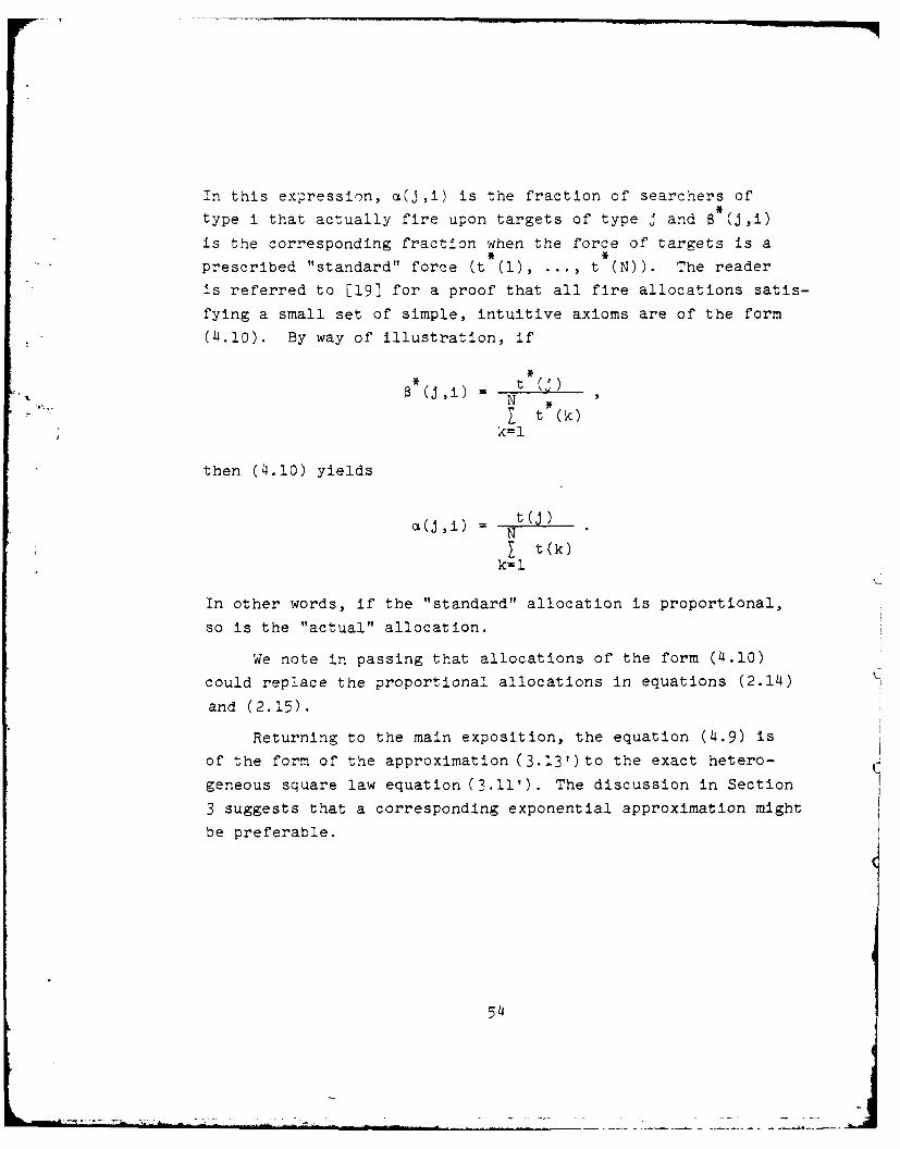
In this expression, a(J,i) is the fraction of searchers of

type i that actually fire upon targets of type j and B (j,i)

is the corresponding fraction when the force of targets is a

prescribed "standard" force (t (1), ..., t (N)). The reader

is referred to [19] for a proof that all fire allocations satis-

fying a small set of simple, intuitive axioms are of the form

(4.10). By way of illustration, if

(i) N ()

E t (k)k=l

then (4.10) yields

t(j)a(J,i) t iN

[ t(k)k=l1

In other words, if the "standard" allocation is proportional,

so is the "actual" allocation.

We note in passing that allocations of the form (4.10)

could replace the proportional allocations in equations (2.14)

and (2.15).

Returning to the main exposition, the equation (4.9) is

of the form of the approximation (3.13')to the exact hetero-

geneous square law equation (3.11'). The discussion in Section

3 suggests that a corresponding exponential approximation might

be preferable.

54

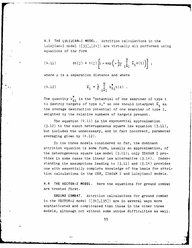
4.3 THE LULEJIAN-I MODEL. Attrition calculations in the;.,ulejian-I model ([33],[24]) are virtually all performed using

equations of the form

(4.11) St(j) = t(j) -exp (- ;1 2is(i))] ,

where p is a separation distance and where

(4.12) kk 1 t= Zi

The quantity k~i is the "potential of one searcher of type ito destroy targets of type Z," so one should interpret k as

ithe average destruction potential of one searcher of type i,weighted by the relative numbers of targets present.

The equation (4.11) is the exponential approximation

(3.12) to the exact heterogeneous square law equation (3.11),but includes the unnecessary, and in fact incorrect, parameter

averaging given by (4.12).

In the three models considered so far, the dominant

attrition equation is some form, usually an approximation, of

the heterogeneous square law model (3.11); only IDAGAM I pro-vides in some cases the linear law alternative (3.14). Under-

standing the assumptions leading to (3.11) and (3.14) provides

one with essentially complete knowledge of the basis for attri-

tion calculations in the CEM, IDAGAM I and Lulejian-I models.

4.4 THE VECTOR-2 MODEL. Here the equations for ground combat

are treated first.

GROUND COMBAT. Attrition calculations for ground combatin the VECTOR-2 model ([34],[35]) are in several ways more

sophisticated and complicated than those in the other three

models, although not without some unique difficulties as well.

55

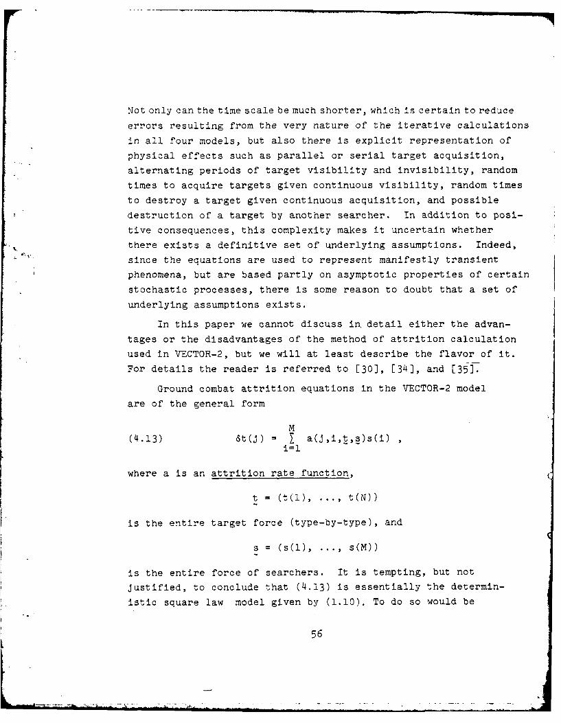
Not only can the time scale be much shorter, which is certain to reduce

errors resulting from the very nature of the iterative calculations

in all four models, but also there is explicit representation of

physical effects such as parallel or serial target acquisition,

alternating periods of target visibility and invisibility, random

times to acquire targets given continuous visibility, random times

to destroy a target given continuous acquisition, and possible

destruction of a target by another searcher. In addition to posi-

tive consequences, this complexity makes it uncertain whether

there exists a definitive set of underlying assumptions. Indeed,

since the equations are used to represent manifestly transient

phenomena, but are based partly on asymptotic properties of certain

stochastic processes, there is some reason to doubt that a set of

underlying assumptions exists.

In this paper we cannot discuss in. detail either the advan-

tages or the disadvantages of the method of attrition calculation

used in VECTOR-2, but we will at least describe the flavor of it.

For details the reader is referred to [30], [34], and [35].

Ground combat attrition equations in the VECTOR-2 model

are of the general form

M(4.13) 6t(j) = [ a(j,i,t,s)s(i)

i1l

where a is an attrition rate function,

t = (t(1), ... , t(N))

is the entire target force (type-by-type), and

s = (S(1), ... , s(M))

is the entire force of searchers. It is tempting, but not

justified, to conclude that (4.13) is essentially the determin-

istic square law model given by (1.10). To do so would be

56

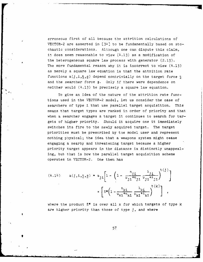
erroneous first of all because the attrition calculations of

VECTOR-2 are asserted in [34] to be fundamentally based on sto-

chastic considerations. Although one can dispute this claim,

it does seem reasonable to view (4.13) as a modification of

the heterogeneous square law process with generator (2.13).

The more fundamental reason why it is incorrect to view (4.13)

as merely a square law equation is that the attrition rate

functions a(j,i,t,s) depend nontrivially on the target force t

and the searcher force s. Only if there were dependence on

neither would (4.13) be precisely a square law equation.

To give an idea of the nature of the attrition rate func-

tions used in the VECTOR-2 model, let us consider the case of

searchers of type i that use parallel target acquisition. This

means that target types are ranked in order of priority and that

when a searcher engages a target it continues to search for tar-

gets of higher priority. Should it acquire one it immediately

switches its fire to the newly acquired target. The target

priorities must be prescribed by tne model user and represent

nothing physical; the idea that a weapons system might cease

engaging a nearby and threatening target because a higher

priority target appears in the distance is distinctly unappeal-

ing, but that is how the parallel target acquisition scheme

operates in VECTOR-2. One then has

(4.14) a(j,i,t,s) = atji j (l - Jiji J) 31 ~1 ~1 J +nJ i Il +X Jl

1 ki xt(k)

+kiki 11ki+Xkit

where the product a* is over all k for which targets of type k

are higher priority than those of type J, and where

57

= mean length of visible periods for one target oftype J and one searcher of type i,

n. - mean length of invisible periods for one target oftype I and one searcher of type i,

= mean time required for one searcher of type i toacquire one target of type J, given continuousvisibility,

OLi = mean time required for one searcher of type i todestroy one target of type J, given continuousacquisition.

The three factors on the right-hand side of (4.14) may be inter-

preted as the kill rate, the probability that a type j target is

visible and acquired (and is hence under attack), and the proba-

bility that no higher priority target is visible and acquired.

We refer the reader to [6], [30], and [34] for details of the

interpretation. Note, however, the following anomaly: as

aJi , , a(j,i,t,s) , which is not sensible. As aJi ) c '

target destruction consumes a negligible amount of time, but

target destruction should not occur at an infinite rate since

it would still be limited by both invisibility and loss of

acquisition.

For descriptions of attrition rate functions for searcherswith serial target acquisition we refer the reader to [30],

[34], and [35].

AIR COMBAT. Attrition in air-to-air combat is calculated

in the VECTOR-2 model using equations of the form

( 4 .5 ) t ( ) . t ( J ) M

) t(j= c(J,i) min {t(J),m,} s(i)

where the c(J,i) are positive constants, interpreted in [341] as"attrition caused by one [searcher] of type i that engages only[targets] of type J," and where mi is the maximum number of

targets that a searcher of type i can engage simultaneously.

58

The equation (4.15) is a linearized approximation to one heter-

ogeneous version (there are several heterogeneous versions that

make sense) of the "Homogeneous Linear Law Process, Multiple

Shot Version" described in Section 3. To fully justify this

assertion would require an unreasonable amount of space and

additional equations, which is not merited at this point in

the paper. The unconvinced reader can find some details in

134] and [35]. Validity of the approximation (4.15) is

questionable in the theater-level context, even for the rela-

tively smaller pieces into which engagements are decomposed

in VECTOR-2, and lack of an exact equation and a set ofunderlying assumptions are significant shortcomings of thc

model.

To conclude this section, we observe once again that the

simplified attrition models treated in Section 3 includenearly all the equations used in four principal theater-level

simulations of ground-air combat. The assumptions set forthin Section 3 contribute much to understanding differences andsimilarities among the attrition calculations in these four

models.

59/AD

5. CONCLUSION

In this paper we have surveyed several aspects of the

theory and applications of Lanchester models of combat, begin-

ning with the original deterministic systems of differential

equations, continuing through continuous time Markov process

analogues, proceeding to simplified stochastic models, and

concluding with a discussion demonstrating that virtually all

attrition calculations in four principal ground-air combat

models are performed using one of the simplified stochastic

models or an approximation to one of the simplified stochastic

models. The approach and philosophical basis of this paper are

distinctive in seeking to illuminate the nature of the various

attrition models in terms of sets of underlying assumptions.

Analysis and understanding of assumptions can only lead to

more enlightened use of models.

6116

REFERENCES

[1] Anderson, L.B., Bracken, J., Healy, J.G., Hutzler, M.J.,and Kerlin, E.P. IDA Ground-Air Model I (IDAGAM I),Volume 1: Comprehensive Description. R-199, Institutefor Defense Analyses (Arlington, Virginia, 1974).

[2] Anderson, L.B., Bennett, D., and Hutzler, M.J. itodifica-tions to IDAGAM I. P-1034, Institute for Defense Analyses(Arlington, Virginia, 1974).

[3] Anderson, L.B., Blankenship, J.W., and Karr, A.F. AnAttrition Model for Penetration Processes. P-1148,Institute for Defense Analyses (Arlington, Virginia, 1976).

[4] Anderson, L.B. Antipotential Potential. N-845, Institute

for Defense Analyses (Arlington, Virginia, 1979).

[5] Anderson, L.B. Attrition Papers Referenced in IDAGAM I.N-846, Institute for Defense Analyses (Arlington, Virginia,1979).

[6] Bonder, S., and Farrell, R. (eds). Development of Modelsfor Defense Systems Planning. SRL-2147 TR70-2, SystemsResearch Laboratory, University of Michigan (Ann Arbor,Michigan, 1970).

[7] Bracken, J. Two Interpretations of Lanchester Processes.Presented at the Conference on Mathematical Models ofConflict and Combat: Theory and Uses. (Mt. Kisco, NewYork, 1979).

[8] Cinlar, E. Introduction to Stochastic Processes.(Prentice-Hall, Englewood Cliffs, New Jersey, 1975).

[9] Clark, G.M. The Combat Analysis Model. Ph.D. dissertation,Ohio State University (Columbus, Ohio, 1969).

[10] Comptroller General of the United States. Report toCongress. Models, Data and War: A Critique of theFoundation for Defense Analysis. PAD-80-21, General

4Accounting Office (Washington, D.C., 1980).

63

t

[11] Deitchman, S.J. A Lanchester Model of Guerrilla Warfare.Operations Research 10(1962) 818-827.

[12] Dolansky, L. Present State of the Lanchester Theory ofCombat. Operations Research 12(1964) 344-358.

[13] Goldie, C.M. Lanchester Square-law Battles: Transientand Terminal Distributions. Journal of Applied Probability14(1977) 604-610.

[14] Helmbold, R.L. A "Universal" Attrition Model. OperationsResearch 14(1966) 624-635.

[15] Jakobovits, R.H. A Class of Simultaneous Point Fire Attri-tion Models. Unpublished memorandum, Institute for DefenseAnalyses (Arlington, Virginia, 1977).

[16] Jennings, N. The Mathematics of Battle III: ApproximateMoments of the Distribution of States of a Simple Hetero-geneous Battle. M-7315, Defence Operational AnalysisEstablishment, U.K. (1973).

[17] Jennings, N. The Mathematics of Battle IV: StochasticLinear Law Battles. M-7316, Defence Operational AnalysisEstablishment, U.K. (1973).

[18] Karlin, S., and Taylor, H.J. A First Course in Stochas-tic Processes, 2nd Edition (Academic Press, New York,1976).

[19] Karr, A.F. Stochastic Attrition Processes of LanchesterType. P-1030, Institute for Defense Analyses (Arlington,Virginia, 1974).

[20] Karr, A.F. A Class of Binomial Attrition Processes.P-1031, Institute for Defense Analyses (Arlington,Virginia, 1974).

[21] Karr, A.F. On Simulations of the St-chastic, HomogeneousLanchester Square Law Process. P-1112, Institute forDefense Analyses (Arlington, Virginia, 1975).

[22] Karr, A.F. On Simulations of the Stochastic, HomogeneousLanchester Linear Law Process. P-1113, Institute forDefense Analyses (Arlington, Virginia, 1975).

[23] Karr, A.F. Deterministic Approximations of Some Stochas-tic Models of Competing Populations. Technical Report239, Department of Mathematical Sciences, The JohnHopkins University (Baltimore, Maryland, 1976).

64

[24] Karr, A.F. On the Lulejian-I Combat Model. P-1l82,Institute for Defense Analyses (Arlington, Virginia,1976). See also Karr, A.F. Additional Remarks on Attri-tion and FEBA Movement Calculations in the Lulejian-ICombat Model. P-1277, Institute for Defense Analyses(Arlington, Virginia, 1977).

[25] Karr, A.F. On the CONAF Evaluation Model. P-1210,Institute for Defense Analyses (Arlington, Virginia,1976).

[26] Karr, A.F. A Class of Lanchester Attrition Processes.P-1230, institute for Defense Analyses (Arlington,Virginia, 1976).

[27] Karr, A.F. A Review of Seven DOAE Papers on MathematicalModels of Attrition. P-1249, Institute for DefenseAnalyses (Arlington, Virginia, 1977).

[28] Karr, A.F. On the IDAGAM I Combat Model. P-1265,Institute for Defense Analyses (Arlington, Virginia,1977).

[29] Karr, A.F. A General Multiple Shot Binomial AttritionProcess. WP-l, Project 2371, Institute for DefenseAnalyses (Arlington, Virginia, 1977).

[30] Karr, A.F. Review and Critique of the VECTOR-2 CombatModel. P-1315, Institute for Defense Analyses (Arlington,Virginia, 1977).

[31] Lanchester, F.W. Aircraft in Warfare: The Dawn of theFourth Arm. No. V, The Principle of Concentration.Reprinted in J. Newman, ed., The World of ,athematics,Volume 4 (Simon and Schuster, New York, 1956).

[32] Louer, F.E., et al. Conceptual Design for the Army inthe Field Alternative Force Evaluation. CONAF Evalua-tion Model IV. OAD-CR-GO, General Research Corporation(McLean, Virginia, 1974).

[33] LuleJian and Associates. The Lulejian-I Theater LevelCombat Model, Volume II: Model Logic and Equations.REIort 259, Weapons Systems Evaluation Group (Arlington,Virginia, 1974).

[34] Miller, G., ed. The V7CTOR-2 Theater-Level Combat Model,Volume I: Users Manual and Volume II: Program Mainten-ance Manual. VRI WSEG-4,5 FR-77-1(R), Vector Research,Incorporated (Ann Arbor, Michigan, 1977).

65

[35] Miller, G., et al. The VECTOR-2 System for Simulation o'Theater-Level Combat, I and II. VRI CCTC-l FR77-1, VectorResearch, Incorporated (Ann Arbor, Michigan, 1978).

[36] Morse, P.M., and Kimball, G.E. Methods of OperationsResearch. (MIT Press, Cambridge, Massachusetts, 1951).

[37] Perla, P.P., and Lehoczky, J.P. A New Approach to theAnalysis of Stochastic Lanchester Processes: I. TimeEvolution. Technical Report 135, Department of Statis-tics, Carnegie-Mellon University (Pittsburgh, Pennsyl-vania, 1977).

[38] Perla, P.P. Approximation Techniques and Optimal DecisionMaking for Stochastic Lanchester Models. TechnicalReport 137, Department of Statistics, Carnegie-MellonUniversity (Pittsburgh, Pennsylvania, 1978).

[39] Snow, R.N. Contributions to Lanchester AttritionTheory. RA-15078, RAND Corporation (Santa Monica,California, 1948).

[40]. Springall, A. Contributions to Lanchester Combat Theory.Ph.D. dissertation, Virginia Polytechnic Institute andState University (Blacksburg, Virginia, 1968).

[41] Sternberg, S.R. Development of Optimal Allocation Strate-gies in Heterogeneous Lanchester Type Processes. Ph.D.dissertation, University of Michigan (Ann Arbor, Michigan,1970).

[42] Taylor, J.G. Lanchester-Type Models of Warfare and Opti-mal Control. Naval Research Logistics Quarterly 21(1974)79-106.

[43] Taylor, J.G., and Brown, G.G. Canonical Methods in theSolution of Variable Coefficient Lanchester-Type Equationsof Modern Warfare. Operations Research 24(1976) 44-69.

[44] Taylor, J.G. Recent Developments in the Lanchester Theoryof Combat. Haley, K.B., ed., Proceedings of the EighthIFORS International Conference on Operations Research(North-Holland, Amsterdam, 1979).

[45] Taylor, J.G. Force-on-Force Attrition Modeling. (Opera-tions Research Society of America, Arlington, Virginia,1980).

66

ILL

>6] Walker, L.G., Higgins, M.S., and Svetlich, W.G. Compari-son and Evaluation of Four Theater-Level Models: CEM IV,:DAGAM I, LUlejian-I, VECTOR-i. Report 299, Weapons SystemsEvaluation Group (Arlington, Virginia, 1976).

>7] Watson, R.K. An Application of Martingale Methods toModels o' Conflict. Operations Research 24(1976)330-382.

48] Weale, T.G. The Mathematics of Battle I: A BivariateProbability Distribution. M-7129, Defence OperationalAnalysis Establishment, U.K. (1971).

'99] Weale, T.G. The Mathematics of Battle II: The Momentsof the Distribution of Battle States. M-7130, DefenceOperational Analysis Establishment, U.K. (1971).

r

[50] Weale, T.G. The Mathematics of Battle V: HomogeneousBattles with General Attrition Functions. M-7511,Defence Operational Analysis Establishment, U.K. (1975).

[51] Weale, T.G. The Mathematics of Battle VI: The Distribu-t-on of the Duration of Battle. M-76126, Defence Opera-.tional Analysis Establishment, U.K. (1976).

[52] Weale, T.G., and Peryer, E. The Mathematics of BattleVII: Moments of the Distribution of States for a BattleWith General Attrition Functions. M-77105, DefenceOperational Analysis Establishment, U.K. (1977).

[53] Weiss, H.K. Lanchester-Type Models of Warfare. Davies,M., Eddison, R.T., and Page, T., (eds.) Proceedings ofthe First International Conference on Operational Research(Operations Research Society of America, Baltimore,Maryland, 1955).

67

9