Embed Size (px)
Citation preview

LIBRARY, CODE 0212 NAVAL, FOSTG?.AjrATE SCHOOL MONTEREY, CALIF. 93940
fy\>7t*S$L
PAPER P-1030^
STOCHASTIC ATTRITION MODELS OF LANCHESTER TYPE
Alan F. Karr
June 1074
INSTITUTE FOR DEFENSE ANALYSES . ^ROGRAM ANALYSIS DIVISION
IDA Log No. HQ 74-16361 CopjJ.sJjpf 190 copies

The work reported in the publication was conducted under IDA'S Independent Research Program. Its publication does not imply endorsement by the Department of Defense or any other govern- ment agency, nor should the contents be construed as reflecting the official position of any government agency.

UNCLASSIFIED SECURITY CLASH riCATioM or THIS RAGE tm,mn o«. »i».»<
REPORT DOCUMENTATION PACE I. RERORT NUMBER
P-1030 J. OOVT ACCESSION NO
4. TITLE fand Subua.)
Stochastic Attrition Models of Lanchester Type
7. »UTMORf«;
Alan F. Karr
». RERP-ORMING ORGANIZATION NAME »MO ADDRESS
Institute for Defense Analyses 400 Army-Navy Drive Arlington. Virginia 22202
II CONTROLLING OFFICE NAME ANO ADORES*
14. MONITORINO AOENCV NAME * AOORESSrif fillmrmnl Intm Controlllnt Ollirm)
READ INSTRUCTIONS BEFORE COMPLETING FORM
1. RECIPIENT'S CATALOG NUMBER
« TrPt or RERORT • RERIOO COVERED
• RIAFORMINO oao. RERORT NUMBER
I CONTRACT OM GRANT NUMBERS)
IDA Independent Research Program io PROGRAM ELEMENT, PROJECT TASK
AREA A «OAK UNIT NUMBERS
II. RERORT 0ATE June 1974
■ I NUMBER Or PAGES 158' It. »IX UNITY CLASS (ml mi. report;
Unclassified IS« OCCLASSiriCATlON DOWNGRADING
SCHEDULE
I«. DISTRIBUTION STATEMENT (ml Ihlm «awlj
This document is unclassified and suitable for public release.
17. DISTRIBUTION STATEMENT (ml »A» mmMtrmct wnlmrmm In »lor» 20. II «IfHMI »POT mmpmn)
II. SUPPLIMtkT*«Y NOTE!
It. KEY WORDS (Cmnllnum on •mvtmm aid. II nmtmmmtr mnä Immnllly my mlmtt number)
Lanchester models, attrition, defense analysis, combat model, stochastic models, Markov attrition processes
10. ABSTRACT (Cmnthmm M HWH mlmt II nmftmry «M» Immnuly my Htm nmmmmt)
The purpose of the research effort summarized in this paper is to give a careful, rigorous, and unified structure to a class of stochastic attrition models originated by F. W. Lanchester. For each of ten attrition processes are stated a concise but complete set of assumptions from which are rigorously derived the form of th« resultant attrition process. These assumptions are "micro" in view- point, concerning the behavior and interaction of individual
DO I JAB"?! MW «OITIOM OF I NOV tl IS OBSOLITf UNCLASSIFIED SECURITY CUASSiriCATlON Or THIS RAGE (»♦••" />«• Knlrrrd)
1

UNCLASSIFIED SECURITY CLASSIFICATION OF THIS PAOKQWlM P« «0
combatants, but are as free from restrictive physical interpre- tation as possible. Each attrition process is a regular step Markov process and is characterized in terms of its jump function, transition kernel, and infinitesimal generator. Also included are several taxonomies of the processes presented, an Appendix of probabilistic technicalities and proofs, and many interpretive remarks. In particular a clarification of the square law-linear law and area fire-point fire dichotomies is given.
UNCLASSIFIED SECURITY CLASSIFICATION OF TNIS PAOEflFh.n Dmlm Bnlmtmd)
I

PAPER P-1030
STOCHASTIC ATTRITION MODELS OF LANCHESTER TYPE
Alan F. Karr
June 1074
IDA INSTITUTE FOR DEFENSE ANALYSES
PROGRAM ANALYSIS DIVISION 400 Army-Navy Drive, Arlington, Virginia 22202
IDA Independent Research Program

TT"
CONTENTS
I INTRODUCTION AND PURPOSE 1
II DETERMINISTIC LANCHESTER ATTRITION THEORY 3
III SOME ASPECTS OF PREVIOUS WORK ON STOCHASTIC LANCHESTER PROCESSES 9
IV STRUCTURE OF THE FAMILY OF PROCESSES DERIVED 13
V A COMPENDIUM OF STOCHASTIC LANCHESTER ATTRITION PROCESSES 21
Al Homogeneous Square Law Area Fire Process 23 51 Homogeneous Square Law Process 27 52 Heterogeneous Square Law Process 29
S3a Heterogeneous Square Law Process 33 53 Heterogeneous Square Law Process 37 LI Homogeneous Linear Law Process 41 L2 Homogeneous Linear Law Process With Engagements ... 43 L3 Heterogeneous Linear Law Process 47 Ml Heterogeneous Mixed Law Process 49
Mia Homogeneous Mixed Law Process 53
APPENDIX: Probabilistic Technicalities and Proofs of Results 55
Al Homogeneous Square Law Area Fire Process 59 51 Homogeneous Square Law Process 67 52 Heterogeneous Square Law Process 81 S3a Heterogeneous Square Law Process 89 53 Heterogeneous Square Law Process 95 LI Homogenous Linear Law Process 101 L2 Homogeneous Linear Law Process With Engagements . . . 107 L3 Heterogeneous Linear Law Process 115 Ml Hetergeneous Mixed Law Process 123 Mia Homogeneous Mixed Law Process 131
REFERENCES 133
in

I. INTRODUCTION AND PURPOSE
The goal of the research effort reported here has been to derive
a class of stochastic attrition models from probabilistic assumptions
on the behavior of individual combatants and on the interactions among
them. Our interest is in stochastic analogs of a family of determin-
istic attrition models commonly called "Lanchester attrition models",
after their originator F. W. Lanchester. These deterministic models
are discussed in Section II.
There are several reasons for undertaking such an effort.
Previous research on stochastic Lanchester models, as surveyed in
Section III, has been concerned mostly with certain computational
problems and in general imposes by hypothesis the form of the attri-
tion process, rather than deriving that form from more elementary
assumptions. In some cases, therefore, our derivations lead to known
and studied processes; the point is that instead of arbitrarily imposed
processes we deal with the consequences of elementary and physically
meaningful hypotheses. In the terminology of economics we employ a
"micro" rather than a "macro" approach, stating assumptions about
individual combatants rather than about the overall form of the
attrition process.
There should be a general preference for stochastic rather than
deterministic attrition models. A stochastic model is more general,
more flexible, more realistic, and better founded, and always provides,
through expectations of its outputs, scalar characterizations of the
system being modeled. Deterministic attrition models of Lanchester
type are represented by differential equations and require allowing
noninteger numbers of combatants, while the stochastic models we
present here have only integer (but vector-valued) states.

The reasons for wishing to derive models from elementary assumptions
are also several. First, one wants to know if there exists a set of
assumptions from which a known process can be derived and, if so, what
physical situations are consistent with the assumptions. Understanding
of the model and its possible applicability are enhanced when assump-
tions are explicitly stated. Different models of combat can be com-
pared in a reasonable manner on the basis of underlying assumptions
(as well as by their relationship to historical data) rather than on
the untenable basis of outcomes, implications, and heuristic judgments.
Once sets of assumptions are in hand, new models may be created
by generalizing or weakening certain assumptions. For example, we
have found that a certain stochastic Lanchester model frequently used
for describing combat between heterogeneous forces is not, based on
underlying assumptions, the appropriate generalization of the corres-
ponding homogeneous model. The effect of weakening unrealistic and
untenable assumptions can be explored in a sensible way only if it
is realized what those assumptions are.
Finally, once underlying assumptions are found for a family of
related processes, one may seek general structural characteristics,
unifying taxonomies, and general computational approaches such as
we present in Section IV.
The final section of this paper is a compendium of the processes
derived so far, giving for each process one family of assumptions
from which it can be derived and a probabilistic characterization of
the process. It may be that certain of these processes can be
derived from alternative sets of assumptions, but we believe that
our families of assumptions are essentially unique.
Probabilistic technicalities and proofs of our results appear in
the Appendix.
The stochastic attrition processes discussed here are all time-
dependent dynamic models with a continuous time parameter. In Karr
(1972a, 1972b, 1973, 1974) similar derivations are given for a
class of static and discrete time attrition models. 2

II. DETERMINISTIC LANCHESTER ATTRITION THEORY
Consider a combat between two homogeneous forces, Blue and Red,
and denote by b(t) and r(t) the numbers of Blue and Red survivors at
time t after the combat is initiated. The British engineer F. W.
Lanchester (1916) suggested that it is the nature of modern warfare
that the instantaneous casualty rate on each side be proportional to
the current strength of the opposing side. Lanchester thus proposed
the now famous model
b'(t) = - c^rCt)
(1) r'(t) = - c2b(t)
where c,, c„ are positive and not necessarily equal. In order that
(1) make sense, the functions b and r must be allowed to assume
arbitrary nonnegative values.
The solution of (1) subject to the initial conditions
b(0) = bQ
r(0) = rQ
is given by
b(t) = bn cosh \t - arQ sinh \t
(2) -i r(t) = rQ cosh \t - a bQ sinh \t
where
X = (c1c2)'
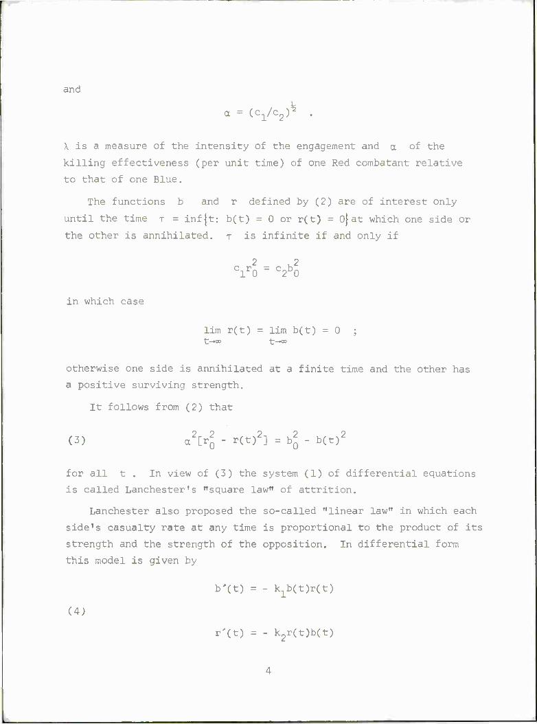
and
a = (c±/c2)
X is a measure of the intensity of the engagement and a of the
killing effectiveness (per unit time) of one Red combatant relative
to that of one Blue.
The functions b and r defined by (2) are of interest only
until the time T = infjt: b(t) = 0 or r(t) = 0}at which one side or
the other is annihilated, T is infinite if and only if
Clr0 = C2b0
in which case
lim r(t) = lim b(t) = 0 ; t—>oo t-*00
otherwise one side is annihilated at a finite time and the other has
a positive surviving strength.
It follows from (2) that
(3) a.2[r20 - r(t)
2] = b20 - b(t)2
for all t . In view of (3) the system (1) of differential equations
is called Lanchester's "square law" of attrition.
Lanchester also proposed the so-called "linear law" in which each
side's casualty rate at any time is proportional to the product of its
strength and the strength of the opposition. In differential form
this model is given by
b'(t) = - kxb(t)r(t)
(4)
r'(t) = - k2r(t)b(t)

where k , k2 are positive constants. These are not the constants of
(1) and, indeed, must have different units. The exact solution to
(4) does not interest us (but note that it is nonnegative, removing
one objection to (2)). The condition analogous to (3) is
r - r(t) = constant x (b - b(t))
from which the term "linear law" originates.
Of considerable interest is the distinction between "square
law" and "linear law" combat. Historically [see, for example,
Bonder (1970, p. 160), Deitchman (1962, p. 818), Dolansky (1964,
p. 345), and Hall (1971, p. 8)] the belief has been that the square
law describes combat situations in which individual opponents are
identified and engaged one-by-one, a situation commonly referred
to as "point fire" combat. On the other hand, the linear law has
been thought to describe combat processes in which weapons (such as
artillery) fire only at an area in which opponents are located
("area fire"). The research presented here leads to a number of
relevant conclusions, whose overall effect in the preceding
distinction is somewhat ambiguous. Indeed, perhaps the best
distinction is the following. "Square law" and "linear law" are
terms which distinguish two types of engagement initiation. In
the former one side initiates engagements (i.e., fires shots) at
a mean rate which is proportional to its own numerical strength
and independent of the numerical strength of the opposition, while
in the latter each side initiates engagements at a mean rate pro-
portional to the product of its numerical strength and that of the
opposition. On the other hand the "area fire" - "point fire"
distinction seems to involve mostly what can happen once a shot
is fired. Area fire processes allow multiple kills with one shot
while point fire processes allow at most one kill by a single shot.
This dichotomy is not unambiguous; for example certain processes
which seem physically to represent the "firing at an occupied area"
aspect usually associated with area fire may in fact have at most
one kill per shot, due to dispersion of one side or the other.
5

Seen in this way the square law-linear law and point fire-area
fire are not competing distinctions but, rather, are complementary,
so that in fact four classes of processes are defined by this classi-
fication scheme.
Let us now consider the case of heterogeneous forces, where
each side consists of two or more distinct types of combatants.
Suppose there are M types of Blue weapons (combatants) and N
types of Red weapons and denote by b.(t) and r.(t) the number of
Blue type i and Red type j weapons, respectively surviving at
time t . Let b(t) = (b^t), ..., bM(t)) and r(t) = (r^t), ...,
r (t)) be the vectors of Blue and Red surviving forces at time t,
respectively.
Since there is no known set of precise and unambigous assumptions
leading by means of a rigorous mathematical derivation to (1) (Weiss
(1957) is typical of the ambiguity and vagueness of previous sets
of assumptions and the lack of rigor of previous derivations) it is
not clear what should be the appropriate generalization to the
heterogeneous case. The usual heterogeneous version of (1) is
obtained purely formally, by replacing b, r, c1 and c2 there by the
vector b, the vector r and matrices c and c^ to obtain the model
N
(5)
bf(t) = - E c (i, j)r (t) , i = 1, ..., M j=l 3
M r'(t) = - E c2(j, i)b.(t) , j = 1, ..., N J 1=1
which is often abbreviated in matrix form as
b' = - c r
c2b ,
where c = [c (i, j)] and c = [c (j, i)] are M x N and N x M non-
negative matrices, respectively.

Evidently there exist neither a closed-form solution to (5) nor
any means of handling negative components. The termination rule so
easily described for the homogeneous square law model (1) does not
carry over. Another of our discoveries is that the stochastic attri-
tion process whose analog is (5) is not, based on sets of assumptions,
the appropriate generalization to the heterogeneous case of the sto-
chastic process analogous to (1). Hence the common practice of
calling (5) "heterogeneous Lanchester-square combat" is unjustified.
As part of our research we have derived the proper stochastic and
deterministic heterogeneous square law models, which are presented
in Section V.
Relatively little has been said about heterogeneous versions of the
linear law model (4) although it has been suggested by D. Howes (per-
sonal communication to L. B. Anderson) that the appropriate form is
N bT(t) =-bi(t) S k (i, j)r.(t)
1=1 J
(6)
r:(t) =-r (t) £ k2(j, i)b.(t) M
where k , k_ are nonnegative M x N and N x M matrices, respectively.
What the motivation for (6) is, other than (4) and intuition, is
not clear, but it does turn out that the stochastic version of ( 6)
is the proper generalization, based on assumptions, of the stochastic
version of (4).
The symmetry of (1) and (4) is not necessary. One might assume
instead that
b'(t) = - cr(t)
(7)
r'(t) = - kb(t)r(t) ,

for positive constants k and c , which is the so-called "mixed-
law,f of Lanchester combat. The mixed law was proposed by Deitchman
(1962) as a model of guerrilla ambushes, with Blue representing the
ambushers and Red the ambushed.

III. SOME ASPECTS OF PREVIOUS WORK ON STOCHASTIC LANCHESTER PROCESSES
We do not intend here to survey in detail the large collection of
previous studies of stochastic models purported to be the proper analogs
of the deterministic systems (1), (4), (5), (6) and (7), except by
indicating the philosophical and mathematical differences between those
approaches and our approach here. The two most extensive published
surveys are Dolansky" (1964) and Hall (1971); Springhall (1968) also
contains a survey and a rather extensive bibliography. Included in
the list of references are a number of papers of interest in the
historical development of Lanchester theories of combat; in particu-
lar, the papers of Brown (1955), Isbell and Marlow (1956) and Weiss
(19 57) contain the germs of the theory. Sets of assumptions in these
early works are imprecise and ambiguous and derivations are, for the
most part, incomplete or nonexistent. One purpose of this research
is to provide consistent and unambiguous sets of assumptions from
which certain stochastic attrition models can be rigorously derived.
In doing so we have unified and extended the theory of Lanchester
combat models.
In order to understand the attrition processes presented in
Section V, some background concerning a certain class of Markov
processes, namely regular step processes, is required; we shall also
make use of the following discussion in the remainder of this section.
Blumenthal and Getoor (1968), Freedman (1971), and Karlin (1968) are
principal references.
Let E be a countable set. A Markov matrix on E is a mapping
P: E x E - [0, 1] with the property that

Z P(i, j) = 1 jeE
for all i e E.
Given a Markov matrix P on E such that P(i, i) = 0 for all i
and a function X : E - [0, ») there exists a Markov process (Xt). n
with state space E satisfying the following intuitive description.
If X(i) = 0, then once the process enters state i it remains there
forever after, while if X(i) > 0 the process, upon entering state i ,
remains there an exponentially distributed time with mean 1/X(i)
independent of the past history of the process, whereupon it jumps
to another state in E according to the probability distribution
P(i, '), independent of the length of its sojourn in state i. (Xx.)
is called the regular step process with jump function X and
transition kernel P .
The family (P.). n of Markov matrices on E defined by
Pt(i, j) = p|xt = j|XQ = if
is called the transition function of (X. ) The matrix-valued mapping
P can be shown to be differentiable and the matrix-
Q = p;
has the property that P' = QP for all t . Q is called the
infinitesimal generator of the regular step process (X. ) and is
given by
(8) Q(i, j) =
- X(i) if j = i
X(i)P(i, j) if j i i .
Q has the interpretation of specifying the "infinitesimal" or
"differential" behavior of the process (Xt) because for j ^ i,
10

Q(i, j) is the "infinitesimal rate" at which the process (X )
moves from state i to state j in the sense that
P{Xt+h = j|Xt = i] = Q(i, j) h + o(h)
as h - 0. Here lim o(h)/h = 0. The resemblance to a system of hiO
differential equations is evident, so a given stochastic attrition
process is called an analog or version of one of the deterministic
models (1), (4), (5), (6), or (7) provided its infinitesimal
generator sufficiently resembles the appropriate system of differ-
ential equations. Further details are in the Appendix.
For example, the second stochastic attrition process presented
in Section IV has infinitesimal generator Q given by
Q((i, j); (i, j - D) = icx
(9) Q((i, j); (i, j)) = - (icx + jc2)
Q((i, J); (i - 1, J)) = 3C2
where c,, c? are positive constants derived from quantities given in
the appropriate family of assumptions. The first equation in ( 9 )
says, in the differential interpretation of Q, that when Blue and
Red strengths are i and j , respectively, Red casualties (that
is the transition from j Red survivors to j - 1 Red survivors) are
occurring at infinitesimal rate ic, . Hence there is justification
for calling the process whose infinitesimal generator is the Q, of
(9), a stochastic homogeneous square law attrition process, because
of the clear resemblance between (1) and (9). This justification,
incidentally, is far from new, dating at least to Snow (1948).
All previous work on stochastic Lanchester-type processes begins
essentially at (9) by imposing as a hypothesis the form of the
generator of the process to be studied. Such studies have generally
been concerned with computing quantities of interest such as
11

(1) expected numbers of survivors at each fixed time;
(2) distribution and expectation of the time required
to reach certain subsets of the state space (such
as the set{(i, j): i = 0 or j = Of of absorbing states
which is entered when one side or the other is anni-
hilated);
(3) the probability that Blue wins the engagement by
exterminating Red.
Our concern has been directed at a more fundamental problem. It
is elementary to show, for example, that there exists a regular step
process whose infinitesimal generator is the Q, given in (9), but
no one has previously presented a complete and unambiguous set of
assumptions on the firing behavior and interaction (or lack thereof)
among combatants which entail an attrition process whose infinitesimal
generator is the Q of (9). It is this lack of basic and physically
meaningful sets of underlying assumptions that this research attempts
to alleviate.
Hence in some cases the processes we derive are known, but not
always. In all cases, it is the derivation and the more primitive
level of the underlying assumptions which are new. Sometimes one
set of assumptions leads the way to a new process (in particular
this is the case for the stochastic versions of the heterogeneous
square law (5)) and these new processes are also discussed in
Section V.
12

IV. STRUCTURE OF THE FAMILY OF PROCESSES DERIVED
We discuss in this section several unifying structures and taxon-
omies which can be applied to the family of stochastic attrition
processes presented in the next section, from which the reader hope-
fully can obtain both overview and insight.
The first taxonomy classifies the stochastic attrition processes
presented here in terms of three criteria:
(1) Multiple kill (area fire) or single kill (mainly point fire)
(2) Square law engagement initiation or linear law engagement
initiation
(3) Homogeneous or heterogeneous force compositions
This appears in Table 1 below. The classification as to type of en-
gagement initiation is based on analogy between infinitesimal genera-
tors of the process and the various systems of differential equations
appearing in Section I.
In each instance the homogeneous model is a special case of the
heterogeneous model and each heterogeneous process correctly reduces
to the corresponding homogeneous process when each side consists of
only one type of combatant.
The second taxonomy is based on the families of assumptions under-
lying the processes, which are presented in Section V. The taxonomy
appears in Table 2, which gives for each of the processes the form of
the basic assumptions from which it is derived (except assumption (3)
which holds for all of the processes). A typical family consists of
(1) An assumption that either
(a) Times between shots fired by a surviving weapon are
independent and identically exponentially distributed
with some mean, that when a shot is to occur exactly
one opponent is detected, attacked, killed or not, and
lost from contact, all instantaneously; or
13

Table 1. TAXONOMY OF THE PROCESSES
Force Composition
Engagement Initiation
Homogeneous Heterogeneous
I. Multiple kill (area fire)
Square law 1) Process Al, a new process with multiple kills and square law engagement initiation
II. Single kill (mainly point fire)
Square law 1) Process SI, whose genera- tor is analogous to (1)
1) Process S2, whose genera- tor is analogous to (5)
2) Process S3a, a new process obtained by simple exten- sion of the assumptions of Process SI
3) Process S3, a new family of processes incorpora- ting fire allocation, of which S3a is a special case
Linear law 1) Process LI, whose genera- tor is analogous to (4)
2) Process L2, a new process generalizing Process LI by the inclusion of engage- ments of positive duration
1) Process L3, a new process obtained by extension of the assumptions of Process LI to the heterogeneous case, with generator analogous to (6)
Mixed law 1) Process Mia, a special case of Ml, with generator analogous to (7)
1) Process Ml, a new process of which a process with generator analogous to (7) is a special case.
14

T^IT-
Table 2. ASSUMPTIONS OF THE PROCESSES
Process
Al Homogeneous Square
SI Homogeneous Square
S2 Heterogeneous Square
Assumptions
la) Mean firing rate is specified.
2) Shot kills binomially distributed number of opponents.
la) Mean firing rate is specified. 2) Shot kills exactly one opponent with probability
p, none with probability 1 - p.
la) One firing process for each opposing weapon type with rate dependent on target and shooter; all such processes occur simultaneously and independently.
2) Kill probabilities depend on target and attacker.
S3 Heterogeneous Square
la) Each shooting weapon fires shots at mean rate dependent only on its type. Allocation of fire over opposing weapon types is by prescribed probability distributions.
2) Kill probabilities depend on target and attacker.
S3a Heterogeneous Square
la) Same as S3 except that fire allocation is by uniform distributions (special case).
LI Homogeneous Linear lb) Mean time to make one-on-one detection specified,
2) Kill probability specified.
L2 Homogeneous Linear
lb) As in LI. 2) Engagement is one-on-one, lasts for exponential-
ly distributed duration, ends with death of one, the other, or neither combatant with specified probabilities.
L3 Heterogeneous Linear
lb) Mean detection time depends on target and searcher.
2) Kill probability depends on attacker and target.
Ml Heterogeneous Mixed
Mia Homogeneous Mixed
1) Each side possesses two weapon types, one of which behaves according to la) and the other according to lb).
2) Kill probability depends on target and attacker.
1) One side has weapons described by 12); the single weapon type on the other side is described by lb),
2) Kill probability specified.
15

(b) The time required to detect a particular opponent is
exponentially distributed with some mean, different
opponents are detected independently, and every
opponent detected is instantaneously attacked, killed
or not, and lost from contact;
(2) Specification of necessary conditional probabilities of
kill given detection and attack;
(3) An assumption that firing processes of all combatants are
mutually independent. Thus each weapon operates independently
of all weapons on the other side and all other weapons on its
own side.
In heterogeneous, mixed, area fire (Al) and time-to-kill (1,2)
models, these assumptions are weakened or modified. The heterogene-
ous Process S3 requires additional assumptions concerning allocation
of fire. In heterogeneous processes, mean rates of fire or detec-
tion and kill probabilities depend in general on both target and
shooting weapon types.
The universal independence assumption (3), even though it is
omitted from Table 2, should not be overlooked. It states that
in a probabilistic sense there is no interaction among weapons on
a given side and interaction among weapons on opposing sides only
when a kill occurs. In particular, none of these models is
capable of handling synergistic effects sometimes thought to be
important, except perhaps by artificial (and possibly unjustifiable)
devices such as modifying the initial numbers of weapons of some
types, based on the absence or presence of some other weapon type
before applying one of the attrition models presented here.
We have attempted to keep our assumptions as free from
restrictive physical interpretation as possible, in order to
demonstrate the full range of applicability of each model. For
16

example consider the assumption (1) of Process SI (see Section V)
which states that times between shots fired by a surviving weapon
are independent and identically exponentially distributed. This
assumption is compatible with a number of different physical reali-
zations of combat. One can envision combatants as stationary and
firing at rates dependent only on their own nature (this seems to
be an "area fire" kind of assumption) or as pressing forward in
such a way as to maintain a constant mean rate of engagements with
the opposition. The point is that our assumptions are not unique
in terms of physical situations in which they might be felt to be
satisfied and we have endeavored to state them in terms which make
it easy to verify their plausibility.
The widely held and already mentioned belief in the correspondence
Square Law-**-Point Fire
Linear Law«*-*-Area Fire
is misconceived. Rather, as we have mentioned earlier, there exists
the following two way classification of processes
Engagement Initiation
Square Law Linear Law
Multiple Kill Structure
Single
which appears to us to make good sense.
17

We may look also at the common properties of the family of
stochastic attrition processes we have derived. Among these
properties are the following:
1) All are regular step processes (in particular, all are
Markovian);
2) Infinitesimal generators resemble the Lanchester differential
models of combat;
3) All components of sample paths are nonincreasing (we have not
included provision for reinforcements);
4) All states are either transient or absorbing (the latter
represent extermination of one side or the other).
Quantities of interest one seeks to compute for use in
modeling attrition would include
1) Expected numbers of survivors (and thus expected attrition)
at various fixed times after the combat begins;
2) The distribution and expectation of first entry times of
various subsets of the state space (which might represent,
for example, breakoff points or extermination of one side);
3) The expected numbers of survivors at random times such as
those in 2) above;
4) Variances of certain quantities, for use in estimating errors
made in computational implementations;
5) In heterogeneous models, expected attrition caused by each
type of opposition weapon.
An advantage of having a family of attrition processes with some
common characteristics is the possibility of developing general com-
putational methods. We will now briefly discuss one which might be
used to compute expected attrition. For concreteness, consider a
18

homogeneous process ((B , R._)V n where B and R are the numbers
of Blue and Red survivors at time t, respectively, With initial
conditions of i Blues and j Reds the expected number of Blue
survivors at time t is given by
i j (10) E[B|(B,R) = (i,j)] = E E kP ((i,j); (k,i))
z u u k=0 1=0 r
where, as will be recalled,
Pt((i,j); (k,£)) = P|(Bt,Rt) = (k,i)|(B0,R0) = (i,j)( .
But by known properties of infinitesimal generators we have
Pr«±, j); (k, £)) = E aQn((i, j); (k, A)) r n=0 n*
where Q is the n power of the infinitesimal generator matrix Q
of the process. Therefore (interchange of the order of summation is
justified by boundedness of all quantities) we can write
ErB.I(Bn,Rn) = (i,j)] = E £r E E kQn((i, j); (k, l)) . r' U U n=0 n* k=0 1=0
00
In particular, the infinite sum E is the limit as M - » of the "n=0
M finite sums E
n=0
Thus for each M we have the approximation
M tn * j n (11) E[B |(B0,R0) = (i,j)] ~ E £r E E k.Q ((i,j); (k,£)) .
u u n=0 n* k=0 j>=0
19
When M = 1 this becomes, provided instantaneous multiple kills are
precluded,
(12) E[Bt|(B0,R0) = (i,j)] ~ i - tQ((i, j); (i - 1, j))
which is essentially the analogous (deterministic) differential
equation. This, incidentally, provides a justification (albeit
tenuous) of using the deterministic differential models as approxi-
mations to the true expectations obtained from stochastic models.
But why choose M = 1 in (11), once the whole family of approxi-
mations (11) is available and justified and when it can even be shown
that each is a better approximation than the preceding one? The matrix
Q consists mostly of zeroes rindeed, Q((i, j); (k, I)) is, in general,
zero unless (k, l) is (i - 1, j), (i, j - 1), or (i, j)] so that it
would be feasible to take M = 3 or 4 or 5 in (11) to produce more
accurate approximations to the true expectations. Moreover, this
scheme of approximation is valid for all the processes we have
derived. The principal difficulty would be computation of powers of
Q. but since Q. consists mostly of zeroes it might well be feasible
to wdiagonalizeM Q ; that is, to find a representation of the form
Q = A_1DA
where D is a diagonal matrix, in which case
^n -l_n,. Q = A D A
becomes trivial to compute and approximations in (11) with M
essentially arbitrary would become feasible. Indeed in this case,
we can obtain P. explicitly as
Pt = A"1 eCD a.
Further research is desirable on such matters.
20

V. A COMPENDIUM OF STOCHASTIC LANCHESTER ATTRITION PROCESSES
We present here the family of attrition process as derived in
this research effort. The format is to give for each process the
set of assumptions from which we have derived it, and a description
of its properties as a regular step process, namely, its jump function,
transition kernel, and infinitesimal generator, followed by inter-
pretive remarks. We also give specific versions of expression (12)
for each process.
We first present some remarks on the general structure of the
families of assumptions leading to the processes described in this
section. Each family includes assumptions concerning the following:
1) Structure of the two opposing forces;
2) The rate at which engagements are initiated;
3) The evolution and possible outcomes of an engagement (in all
processes but L2 an engagement occurs instanteously and can
end only in death of some weapons on the engaged side and
loss of contact);
4) If necessary, allocation of fire;
5) Interaction among weapons on a given side;
6) Interaction of a weapon on one side with weapons on the
opposing side, other than engagement.
In all models, 5) and 6) are independence assumptions stipulating
no interaction.
As general notations we establish Bt for Blue survivors at time t
and R for Red survivors at time t. These will sometimes be vectors.
For each process we give the values of jump function, transition
kernel, and infinitesimal generator only for nonabsorbing states.
21

The set of absorbing states is left to the reader to determine (it is
the family of states in which one side or the other is exterminated).
If x is absorbing X(x) = 0, Q(x, y) = 0 for all y and P(x, .) is
not defined.
??

Al Homogeneous Square Law Area Fire Process
Assumptions
1. All weapons on each side are identical.
2. Times between shots fired by a surviving Blue weapon are
independent and identically exponentially distributed with mean 1/r,.
3. If a shot is fired by a Blue weapon when there are k Reds
surviving the shot has the instantaneous effect of killing a number
of Red weapons which is binomially distributed with parameters
(k, px).
This means that the shot has probability p. of killing each
particular Red weapon and that different Red weapons are killed
independently of one another.
4. Red weapons satisfy assumptions 2 and 3 with mean time between
shots l/r2 and individual target kill probability p?.
5. Firing processes of all weapons are mutually independent.
Process Characterization
Under the preceding set of assumptions the stochastic survivor
process ((B. , R1.))1_^0 is a regular step process with jump function
\ given by
\(i, j) = ir^l - (1 - Pl)j) + jr2(l - (1 - pj)1) ,
transition kernel P given by
iri(i)ci - pi)A pi_A
P(fi,j); (i,x)) = ww-,- A\ > i = °> •••> J
.(i,3); (k,j)) = N x(i> j) >
23

and infinitesimal generator Q given by
Q((i, j); (i, JD) = i^fJKl - v^'vi'1: 1=0> ..., j-1
Q((i, j); (i, j)) = -Cir^l - (1 - Pl)J) + jr2(l - (1 - p^1)]
Q((i, 3); (k, j)) = Jr2fjVl - P2)k p^_k, k=0, ...., i-1 •
The binomial distribution of assumption 2 can be replaced by any
probability distribution on 0,...,k , so this process is in fact a
whole class of similar processes. In particular, the distribution
which places mass p, on 1 and mass 1 - p, on 0, yields the Process
SI described below.
This process is in many ways the most interesting of those we
have derived, because of the number of intriguing questions it
raises. The interpretation of its assumptions, especially that
concern binomially distributed multiple kills, seems to be unequi-
vocally that of area fire. (Indeed, the possibility of multiple
kills may well be the distinguishing feature of area fire combat
processes). What is at issue is whether this is a square law
process or a linear law process. Consider its infinitesimal
generator Q. Examining the term - Q((i,j),(i,j)), which is the
rate at which the process leaves state (i,j), we have what appears
to be of square law form (cf. the corresponding term for process
SI). But on the other hand
Q((i,j), (i,j - 1)) = irxj(l - P!)3"1?! ,
which can be thought of as a representation of the instantaneous
rate at which Red combatants are being destroyed when the current
state of the process is (i,j), can be argued to be of linear law
form (but not entirely, because of the presence of the factor
(1 - Pl)j_1)..
One way to clarify the situation is to abandon the square law-
linear law dichotomy for attrition entirely and to simply regard
the processes we have derived, in terms of their underlying
24

assumptions. What distinguishes Process Al from all the other
processes is the provision for multiple kills, so it might even
be argued that this is the only true "area fire" process presented
here. The whole situation is complicated by the fact that if the
binomial distribution of assumption (2) is replaced by the distribu-
tion with mass p on 1 and mass 1 - p on 0 the Process SI, which seems
clearly to be a square law process, is obtained.
25


SI Homogeneous Square Law Process
Assumptions
1. All weapons on each side are identical.
2. Times between shots fired by a surviving Blue weapon are
independent and identically exponentially distributed with mean 1/r...
3. When a shot occurs it kills exactly one Red weapon with
probability p and no Red weapons with probability 1 - p , instan-
taneously and independent of past history of the process.
4. Red weapons satisfy assumptions 2 and 3 with mean time between
shots of l/r„ and kill probability p .
5. The firing processes of all weapons are mutually independent.
Process Characterization
For i = 1, 2,16t c. = r.p.. Then subject to Assumptions 1 to 5
above, ((B , R1_))+_^n is a regular step process with state space
t) xN, jump function \ given by
X(i, j) = ic1 + jc2 ,
transition kernel P given by
icl PC(i, J); (i, J - D) = ic, + jc,
P((i, j); (i - 1, j)) = JC2
IC^ + ]C2 '
and infinitesimal generator Q given by
Q((i, 3), (i, j - D) = ic1
Q((i, J), (i, J)) = - (icx + Jc2)
Q((i, j), (i - 1, j)) = jc2 .
27

For this process the approximation (12) is given by
E[Bt|(B0, R0) = (i, j)] ~ i - jc2t ;
similarly
E[Rt|(BQ, R0) = (i, j)] ~ j - iCjLt .
Clearly the larger t is, the worse the approximation.
By the form of Q this process is the stochastic version of the
deterministic square law (1). 1/c-, is the mean time between fatal
shots fired by a Blue weapon, so c, = r,p, can be interpreted as the
mean rate at which a Blue weapon kills Red weapons (which is inde-
pendent of the strength of the Red force so long as the latter remains
nonzero), giving in physical terms what the coefficients c, and c? in
(1) mean.
28
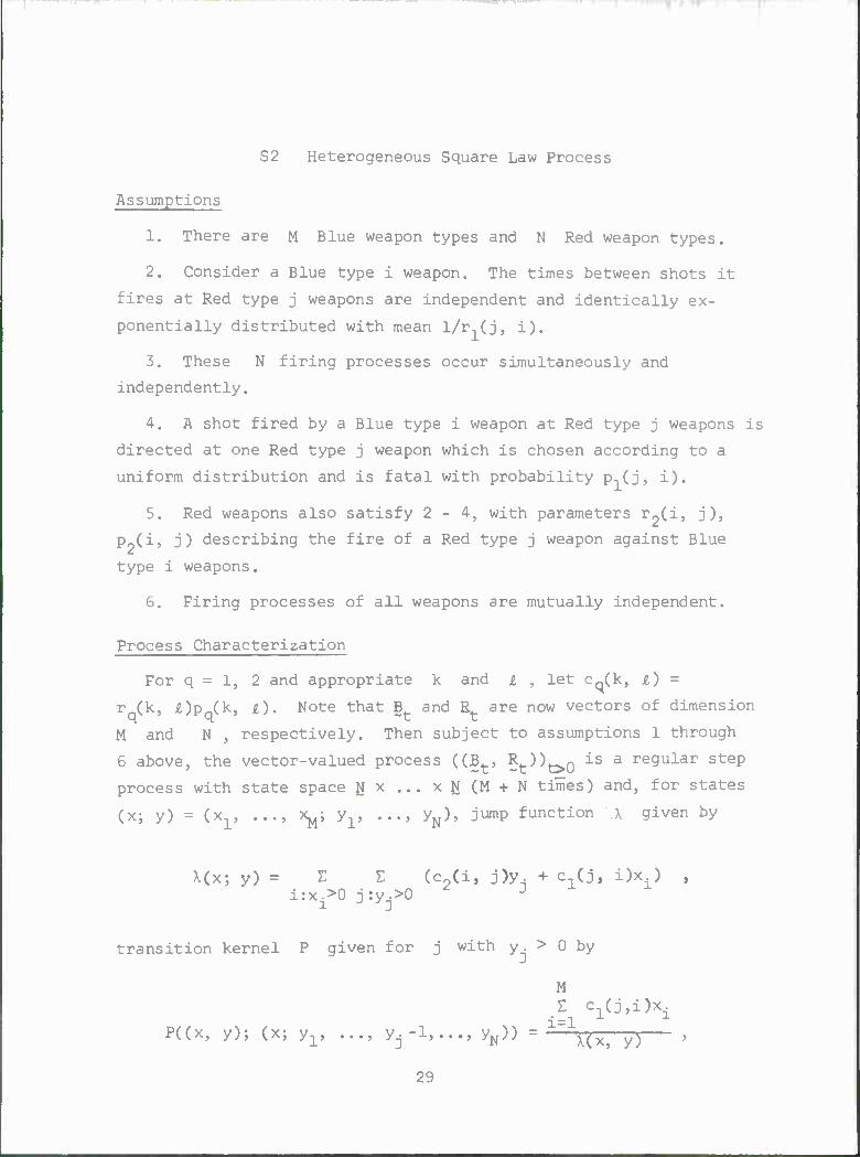
S2 Heterogeneous Square Law Process
Assumptions
1. There are M Blue weapon types and N Red weapon types.
2. Consider a Blue type i weapon. The times between shots it
fires at Red type j weapons are independent and identically ex-
ponentially distributed with mean l/r,(j, i).
3. These N firing processes occur simultaneously and
independently.
4. A shot fired by a Blue type i weapon at Red type j weapons is
directed at one Red type j weapon which is chosen according to a
uniform distribution and is fatal with probability p,(j, i).
5. Red weapons also satisfy 2-4, with parameters r_(i, j),
p9(i, j) describing the fire of a Red type j weapon against Blue
type i weapons.
6. Firing processes of all weapons are mutually independent.
Process Characterization
For q = 1, 2 and appropriate k and l , let c_(k, l) =
r (k, £)p (k, i). Note that B and 1L are now vectors of dimension
M and N , respectively. Then subject to assumptions 1 through
6 above, the vector-valued process ((Bt, f^))^ is a re9ular steP
process with state space N x ... x N (M + N times) and, for states
(x; y) = (xr ..., xM; yp ..., yN), jump function .X given by
X(x; y) = Z % (c?(i, j)y. + c,(j, i)x.) , i:x±>0 j:y.>0 ' J
transition kernel P given for j with y > 0 by
M E c (j,i)x.
i=l P((x, y); (x; y±, ..., y^ -1,..., yN>) = x^x> y^ ,
29

and for i with x. > 0 by
N E c2(i,j)y.
P((x,y); (x1,...,xi-l,...,xM; y)) = 3" x(x>y)
and infinitesimal generator Q given by
M Q((x,y); (x; y^...,^-!, ...,y„)) = _E c1(j,i)xi if y >
Q((x,y); (x,y))= - E E (c (i,j)y i:x.>0 i:y.>0 J
+ c1(j,i)xi)
N Q((x,y);(x1,... xi - l,...,xM; y))= E c2(i,j)y if x. > 0.
' j=l J
State (x,y) is absorbing if and only if x - 0 or y - 0.
Corresponding to the approximation (12) we have for this process
EC5t'^0, R0) =(x,y)] ~ x. - ( £ c2(i, j)y.)t
for i = 1, ..., M while for j = 1, ..., N
M E[R^|(B0, R0) = (x, y)] ~ yj - ( E Cl(j, i)Xi)t .
It seems rather natural to call this process "heterogeneous
Lanchester square" because of resemblance of Q to the system (5)
of differential equations, and this process provides a physical
interpretation of the matrices in (5). But the physical interpreta-
tion of the assumptions is quite unappealing. In particular, assump-
tions 2 and 3 are unpalatable. They state that each weapon carries
out one firing process for each type of opposition weapon and that
30

all these processes are evolving concurrently and independently.
On the contrary, the spirit of assumption 2 of processes Al and
SI is that a weapon's firing behavior is a function only of its
type and of whether there are a positive number of targets present.
The next process we present is in that spirit.
It is, in any case, the present process S2 which is commonly
referred to as "stochastic heterogeneous Lanchester square*. Based
on the structure of the underlying families of assumptions, this
designation seems to be inappropriate.
31


S3a Heterogeneous Square Law Process
Assumptions
1. There are M Blue weapon types and N Red weapon types.
2. Times between shots fired by a surviving Blue type i weapon
are independent and identically exponentially distributed with mean
1/r^i).
3. When a Blue type i weapon fires a shot it is directed at a Red
weapon chosen from all Red weapons currently surviving according to a
uniform distribution.
4. A shot fired by a Blue type i weapon at a Red type j weapon
is fatal with probability pn(j,i).
5. Assumptions 2-4 hold for Red with mean firing rates r?(j)
and kill probabilities p2(i,j).
6. The firing processes of all weapons initially present are
mutually independent.
Process Characterization
Under the preceding family of assumptions, the survivor process
((B , St))t>o is a re9ular steP process with state space £J x ... xjj
(M + N time's), jump function \ given by
M N x. y. X(x,y) = E E [ t
11 P2(i,j)r2(j)y. + ^± p1( j ,i)r1(i)xi]
i=l j=l J y
M N where x • 1 = E x, , y • 1 = E y, transition kernel P given by
M v E p (j,i)r (i)x yj i=i x _____
1» •,,'yj x' *••' yM" :: y • 1 \(x,y)
N v E P2(i,j)r2(j)y. i 3=1 3
3 i i=l P( (x,y); (x; y,,...,y. - 1, ..., y )) =-
P((x,y); (x1,...,xi - 1,...,^; y)) = x ^ X(x,y)
33
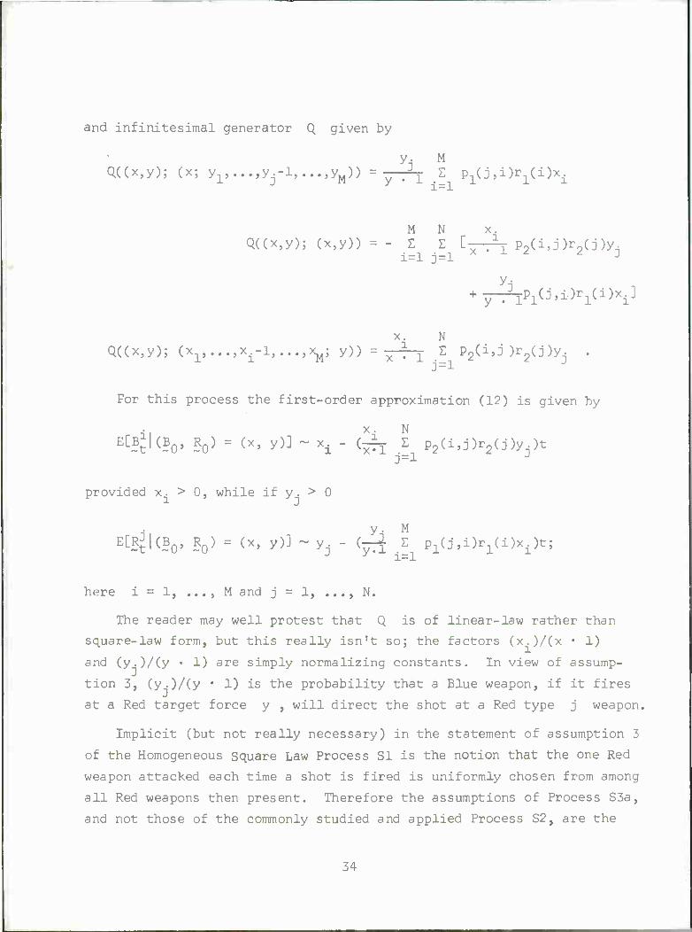
and infinitesimal generator Q given by
yi M Q((x,y); (x; yx,...,yj-l,...,yM)) = J± _E p1(j,i)r1(i)xi
M N x. Q((x,y); (X,y)) = - E E [—K p2(i, j )r (j )y
i=l 1=1 x L * z 3 3:
yi + 7TTpl(j'i)rl(i)xi]
x. N Q((x,y); (xl, ...,xi-l,...,xM; y)) = 7-^3 T, P2(i, j )r2(j )yj .
For this process the first-order approximation (12) is given by
x. N EC?t,(?0> ^ = (x' y)] ~ xi ~ Cx^I E P2(i'^r2(^yi)t
j=l J
provided x. > 0, while if y. > 0
y. M E[R^|(B0, R0) = (x, y)] ~ y - (—1 E p^ j ,i)r (Dx^t;
here i = 1, ..., M and j = 1, ..., N.
The reader may well protest that Q is of linear-law rather than
square-law form, but this really isn't so; the factors (x.)/(x • 1)
and (y.)/(y • 1) are simply normalizing constants. In view of assump-
tion 3, (y-)/(y * 1) is the probability that a Blue weapon, if it fires
at a Red target force y , will direct the shot at a Red type j weapon.
Implicit (but not really necessary) in the statement of assumption 3
of the Homogeneous Square Law Process SI is the notion that the one Red
weapon attacked each time a shot is fired is uniformly chosen from among
all Red weapons then present. Therefore the assumptions of Process S3a,
and not those of the commonly studied and applied Process S2, are the
34

proper generalization of the assumptions of Process SI to the
heterogeneous case. This generalization preserves dependence of mean
firing rate on only the type of the shooting weapon and the uniform
fire allocation. Hence, we believe, it is more appropriate to call
process S3a a stochastic model of heterogeneous Lanchester-square
attrition that it is to so call Process S2.
The system of differential equations analogous to this process is
given by
- r. M r' =nrJ- E kl(j, i)b.
1=1 l
- b. N b^=-TrJ- Z^Ci, j)r.
S b. :
k=l K
where
k-^j, i) = Px(j, i)rx(i)
and
k2(i, j) = PjC1» J)r2(j) •
In particular this provides an interpretation of the matrices k , kj,
35


S3 Heterogeneous Square Law Process
Assumptions
The assumptions here are those of the Process S3a but with
assumption 3 there modified as follows.
3. If a Blue type i weapon fires a shot at a time when the Red
force is (the N-vector) y then the probability that the one target
attacked is of type j is ^(yj), j = 1, ..., N; within the class of
type j targets the specific target attacked is chosen uniformly. For
each i and y , ^(y, • ) is a probability distribution over the
set | 1, ..., N} of Red weapon type indices.
Similarly, assumption 5 is changed to include fire allocation
distributions n..(x, • ) for Red type j weapons firing at a Blue force
of composition x .
Process Characterization
Under the family of assumptions given above, ((B , R )) _ is a
regular step process with jump function X given by
M N X(x,y) = E S U (y,j)p (j,i)r (i)x.
1=1 j=l x 1 x 1
+ ri:).(x,i)p2(i,j)r2(j)y:j},
transition kernel P given by
M E *i(y,j)P1(j,i)r1(i)x:L
P((x,y); (x; y±, ..., y^ - 1, ..., yN)) = ~ \(x,y)
£ T):j(x,i)p2(i,j)r2(j)yj
c, y); x15 ..., x. - i,..., XJJ; y)) =2=1 r(7-y5 , P((x,
and infinitesimal generator Q given by
37

M Q((x,y); (x; y15...,y. - l,...,yN)) = E *.(y,j)P1(j,i)r1(i)xi
J i=l
M N Q((x,y); (x,y)) = - E E | * .(y, j )p (j ,i)r (i)x + r\Ax,i)p (±,j)v (j)yA
i=l j=i x x x 1 j / z j I
N Q((x,y); (x1,...,xi - l,...,^^)) = E r|.(x,i)p2(i, j)r2(j )y. .
j=l
For this process the approximation (12) has the form
i r N l ECBt| CB0, R0) = (x, y)] ~ x. - [. E ^(x, i)p2(i, j )r2( j )y Jt
for i such that x. > 0. Similarly, for j such that y. > 0 we have
r M -l E[RJ|(BQ, R0) = (x, y)] ~ y, - E Y.(y, j)p1(j,i)r1(i)xiJt .
J L i=l
Process S3a is obtained as a special case of Process S3 by taking
♦i<y» j) =7-^T
and x.
for all i and j . The generator Q of Process S3 is clearly of
Lanchester square form, in the sense of resembling (5). Thus, Process
S3a is a square law process. This similarity, incidentally, conveys
additional information about what the coefficients in (5) should mean.
Effects such as target priority and axiomatically derived alloca-
tions are included within the large class of S3 processes. See the
Appendix for details.
38

We note that the system of differential equations analogous to
this stochastic process is given by
M r'(t) = - S Y.(r(t), j)p (j, i)r (i)b.(t) j i=1 i 11
for j = 1, ..., N and by
N br(t) = - £ Y.(b(t), i)p (i, j)r (j)r (t)
3=1 3 L Z 3
for i = 1, ..., M. The reader should be aware of the potentially
confusing notation: the r (i) and r~(j) are mean firing rates while
the r.(t) are surviving Red weapons.
The assumptions for Processes SI, S2, S3 are all clearly similar.
To interpret any of these as an area fire process requires the
following reasoning: since a combatant's mean rate of fire is inde-
pendent of the size of the opposing force, he can be envisioned as
simply firing into an enemy-containing region according to a Poisson
process determined by his own attributes (e.g., weapon, location, ...),
which seems plausible. But it must then be assumed that a shot kills
either exactly one enemy combatant or none, which doesn't seem entire-
ly reasonable. Indeed, we have previously suggested that area fire
attrition processes are distinguished by the possibility of multiple
kills arising from one shot. Hence it can be argued that of all the
processes presented here only the Process Al is an area fire process,
and that all the others are point fire processes which are grouped
into two classes (square-law and linear-law) according to the form
of mean engagement rates. For square-law processes the engagement
rate depends only on the strength of the side initiating engagements,
while for linear-law processes each engagement rate is proportional
to the product of the strengths of the two sides. These, of course,
correspond to rather different physical situations.
39


LI Homogeneous Linear Law Process
Assumptions
1. All weapons on each side are identical
2. The time required for a Blue weapon to detect a particular
Red weapon is exponentially distributed with mean 1/s,. Each Blue
weapon detects different Red weapons independently.
3. A Blue weapon attacks every Red weapon it detects; the
conditional probability of kill given attack is q,. The attack
occurs instantaneously and contact is immediately lost. An attack
cannot occur without a detection.
4. Red weapons satisfy the same assumptions with parameters
s2, q2«
5. The detection and attack processes of all weapons initially
present are mutually independent.
Process Characterization
Let k = s q for l = 1, 2.
Under assumptions 1 - 5,((Bt, Rt)) is a regular step process with
state space N x N, jump function X given by
X(i,j) = iJC^x + k2)
transition kernel P given by
kl P((i,j), (i,J " D)
k, + k2
k2 P((i,j), (i " 1,3)) =k1 + k2
and infinitesimal generator Q given by
>
41
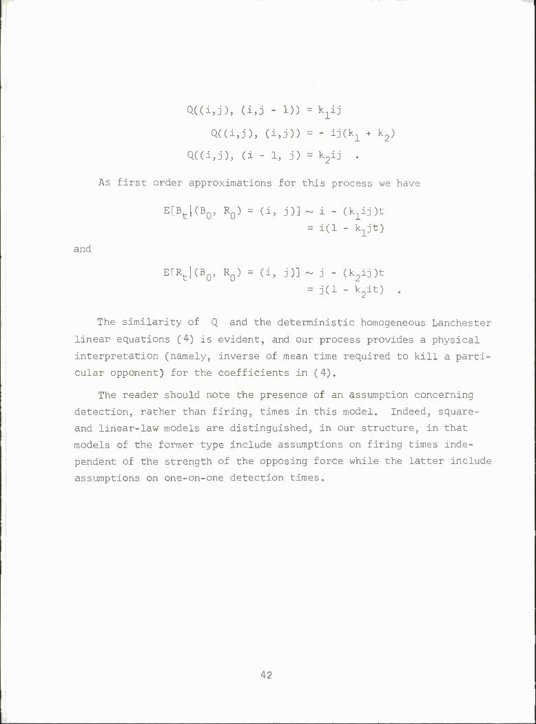
and
Q((i,j), (i,j - D) = \±3
Q((i,j), (i,j)) = - ij(kx + k2)
Q((i,j), (i - 1, j) = k2ij .
As first order approximations for this process we have
ErBt|(BQJ R0) = (i, j)] ~ i - (kxij)t
= i(l - kxjt)
ErRt|(B0, R0) = (i, j)] ~ j - (k2ij)t
= j(l - k2it) .
The similarity of Q and the deterministic homogeneous Lanchester
linear equations (4) is evident, and our process provides a physical
interpretation (namely, inverse of mean time required to kill a parti-
cular opponent) for the coefficients in (4).
The reader should note the presence of an assumption concerning
detection, rather than firing, times in this model. Indeed, square-
and linear-law models are distinguished, in our structure, in that
models of the former type include assumptions on firing times inde-
pendent of the strength of the opposing force while the latter include
assumptions on one-on-one detection times.
42

L2 Homogeneous Linear Law Process With Engagements
Assumptions
1. All weapons on each side are identical.
2. The time required for a Blue weapon to detect a prescribed Red
weapon is exponentially distributed with mean 1/s.. Each Blue weapon
detects different Red weapons independently.
3. A Blue weapon engages every Red weapon it attacks.
4. All engagements are binary (i.e., one-on-one). During an
engagement both combatants are invulnerable to other weapons and unable
to make further detections.
5. The length of an engagement is exponentially distributed with
mean l/u. An engagement terminates in exactly one of the following
outcomes with the probabilities indicated, independent of past history.
Outcome Probability
Blue killed, but not Red p
Red killed, but not Blue p„
Mutual survival p, = 1 - p - p„ .
These parameters are independent of the initiator of the engagement.
6. Red weapons satisfy assumptions 2 and 3, with mean detection
time l/Sp.
7. All detection processes, engagement lengths, and engagement
outcomes are mutually independent.
Process Characterization *
To study this model we define some further notation. Let Bt
denote the number of unengaged Blue weapons at time t, Rt the number
of unengaged Red weapons at time t and D the number of binary engage-
ments in progress at time t, which is also the number of Blue weapons
and Red weapons engaged at time t. We first consider the three component
process ((Bt, Rt, Dt))t>0 • 43

Under assumptions 1 through 7 above, the process ((B*, R*, D )) n
is a regular step process with state space N x N x N, jump function
X given by
Ui,j>k) = ku + ij(s1 + s2) ,
transition kernel P given by
kp u P((i,j,k), (i + l,j,k - 1)) =
ku + ij(s, + s„)
kp u P((i,j,k), (i, j + 1, k - l))-
ku + ij(s1 + s2)
kp u P((i,j,k), (i + l, j + l, k - l)) =
P((i,j,k), (i - l, j - l, k + 1)) =
ku + ij(s1 + s2)
ij(s1 + s2)
ku + ij(s1 + s2) '
and infinitesimal generator Q given by
Q((i,j,k), (i + 1, j, k - 1» = kp2u
Q((i,j>k), (i, j + 1, k - 1)) = kPlu
Q((i,j,k), (i + 1, j + 1, k - 1)) = kp3u
Q((i,j,k), (i - 1, j - 1, k + 1)) = ij(Sl + s2)
Q((i,j,k), (i,j,k)) = - [ku + ij(s1 + s2)] .
From the state of i unengaged Blue weapons, j unengaged Red
weapons, and k engagements in progress, four states may be reached,
corresponding to the events "termination of one engagement with kill
of a Red weapon", "termination of one engagement with kill of a Blue
weapon", "termination of one engagement with mutual survival", and
"initiation of one additional engagement". These occur at the rates
indicated by the expressions for Q (which, as usual, assume that
i>0, j > 0, k>0 and must be suitably adjusted for other states).
Based on its assumptions and the term in Q expressing engage-
ment initiation, this process is of linear law type. But our
44

principal interest is in the survivor process ((B, , R.)) defined by
Bt = B* + Dt
and
Rt=R*+Dt ,
since the number of Blue weapons surviving at time t is the sum of the
numbers of unengaged and engaged Blue weapons surviving at time t, and
similarly for Red. The process ((B , R^)) is not, unfortunately, a
regular step process and we have not yet characterized it in a useful
manner. However, expectations of B^ and R are easy to compute from
those of B£,. R£> and D , because
E[Bt] = E[B*] + E[Dt]
and E[R ] = E[R*] + ErDt] .
The latter expectations might be computed, since ((B*, R*, D )) _
is a regular step process, using the methods described in Section IV.
To compute first-order approximations to E[B ] and E[R ] we first
note that (12) and the form of the generator Q of this process imply
that
E[B*|(B*, R*, D0) = (i,j,k)] ~ i - [ij(s1 + s2) + ku(p2 + p3)]t ,
that
E[R*|(B*, R*5 D0) = (ä,j,k)] ~ j - Tij(s1 + s2) - ku(P;L + p3)]t ,
and also that
E[Dt|(B*, R*5 D0) = (i,j,k)] ~ k - [ku - ij(S;L + s2)]t .
45

Thus
E[Bt|(B*, R*, D0) = (i,j,k)]
= E[B*|(B*, R*, D0) = (i,j,k)] + E[Dt|(B*0, R*, DQ) = (i,j,k)]
~ i - ij(s1 + s2)t + ku(p2 + p3)t + k - kut + ij(s1 + s2)t
= i + k - (p ku)t ;
we similarly obtain
E[Rt|(B*, R*, D0) = (i,j,k)] = j + k - (p2ku)t .
The assumption that the two weapons in a binary engagement be
invulnverable to other opposition weapons is questionable (an engaged
weapon would seem to be relatively more vulnerable than an unengaged
weapon) and alternatives should be sought.
46

L3 Heterogeneous Linear Law Process
Assumptions
1. There are M Blue weapon types and N Red weapon types.
2. The time required for a Blue type i weapon to detect a parti-
cular Red type j weapon is exponentially distributed with mean
l/s-j^Cjji). Each Blue weapon detects different Red weapons independently.
3. A Blue weapon attacks every Red weapon it detects. The condi-
tional probability that a Blue type i weapon kills a Red type j weapon,
given detection and attack, is p1(j,i).
4. Red weapons satisfy assumptions 2 and 3 with mean detection
times l/s?(i,j) and kill probabilities p?(i,j) describing Red type j
weapons opposing Blue type i weapons.
5. Detection and attack processes of all weapons present are
mutually independent.
Process Characterization
For q = 1, 2 and appropriate k and i define k (k,£) =
s (k,£)p (k,jO. Then under assumptions 1 through 5 above, the vector-
valued survivor process ((B Rt))t>n is a re9ular steP process with
state space $} x ... x N (M + N times'), jump function X given by
M N X(x,y) = E Z x.y.[k,(j,i) + k2(i,j)] ,
i=l j=l J
transition kernel P given by M
V3 i=! Vl(j>1)Xi P((x,y); (x; y1,...,y-j - i,...,yN)) = \(x,y)
N x. Z k„(i,j)y.
i=l P((x,y); (x1,...,xi - 1,...,)^; y)) = x,(x,y) ■
47

and infinitesimal generator Q given by
M Q((x,y); (x; y,,...,y. - l,...,yN)) = y. E k,(j,i)x.
j j i=1 J. j
M N Q((x,y); (x,y)) = - E E x y. [k (j,i) + k (i,j)]
i=l j=l x J x *
N Q((x,y); (x1,...,xi - l,...,)^)) = x E k2(i,j)y. .
j=l J
Expectations of numbers of survivors in this process may be
approximated using (12) in the following manner:
i N
E[Bt|(B0, R0) = (x,y)] ~ xi - [x. E k2(i,j)yj]t
j=l
N = x.[l - t E k (i,j)y )]
: j=l J
and
M E[R; ■J|(B0, RQ) = (x,y)] ~ y - [y, E k1(j,i)x/|t
M = y,[i - t s k (j,i)x )1 ,
J i=l x
for i = 1, ..., M and j = 1, ..., N.
Based on its underlying assumptions this process is clearly the
heterogeneous analog of the stochastic homogeneous linear law Process
LI. Its infinitesimal generator Q is similar to the system (6),
which comfirms that (6) is an appropriate deterministic heterogeneous
linear model and provides the proper interpretations of the coeffi-
cients in (6); namely, the inverse of the mean time required to detect
and kill a particular opposition weapon of a given type.
48

Ml Heterogeneous Mixed Law Process
Assumptions
1. Each side possesses exactly two types of weapons.
2. Times between shots fired by a surviving type 1 Blue weapon
are independent and identically exponentially distributed with mean
l/rr
3. Each such shot is directed at a target chosen according to a
uniform distribution on the set of all Red weapons surviving at that
time. If the target is a Red type j weapon it is killed with proba-
bility p1(j).
4. Red type 1 weapons satisfy assumptions 2 and 3 with mean
firing rate r_ and kill probability p2(i) against a Blue target of
type i.
5. The time required for a Blue type 2 weapon to detect a parti-
cular Red weapon of type j is exponentially distributed with mean
l/s-.(j). A fixed Blue type 2 weapon detects different Red weapons
independently of one another.
6. A Blue type 2 weapon attacks every Red weapon it detects.
The conditional probability, given detection and attack, that a Red
weapon of type j is killed, is q-,(j). The attack occurs instan-
taneously and contact is lost.
7. Red type 2 weapons satisfy assumptions 5 and 6 with mean
detection times l/s2(i) and kill probabilities q2(i) against type i
weapons.
8. All weapons detect and attack independently of one another.
Process Characterization
Under assumptions 1 through 8 above, the survivor process
((B1, B^, RL RH))t>0 is a re9ular steP Process with state space
49

N x N x N x N, jump function \ given by
p (l)k + p (2)£ \(i,j,k,£) = irx(-i j_£± )
+ j [ks1(l)q1(l) + £s1(2)q1(2)]
p (l)i + p (2)j + kr2 C 2 i + j )
+ £ [is2(l)q2(l) + js2(2)q2(2)] ,
transition kernel P given by
iripi(1) \TT1 + Jks/Dq (1) P((i,j,k,£); (i.j.k - I,«)« -JLi foj>kt0 ^~
ir p (2) T-A-T + jis (2)q (2) P((i,j,k,i); (i,j,M - 1)) =-AJ: ^ij.k,!) i
kr„p9(l) T-^--r + Ais9(l)q9(l) pcci,j,k,i)j (i - i,j,k,.o) =-AJ—l(
+i}])Ki) —l—
kr p (2) T^—r + jjjs (2)q (2)
p((i,j,k,i); (i,j - i,k,o) =-^—xaJ,k,x)
and infinitesimal generator Q given by
50 ,

T-"
Q((i,j,k,i); (i,j,k - l,i)) = ^^(1)^-—^+ jks (i)q M)
Q((i,J,K,£); (i,j,k,X - 1)) = ±1^(2) ^-i-j + jis1(2)q1(2)
p,(l)k + p,(2)£ Q((i,j,k,4);-(i,j,k,£)) = - { ir^-i rTT± )
+ j[ks1(l)qi(l) + is1(2)q1(2)]
p9(l)i + p?(2)j + kr2 C2 i + j )
+ i[is2(l)q2(l) + js2(2)q2(2)]}
Q((i,j,k,jt); (i - l,j,k,i» = kr2p2(l) ^-i-j + jtis2(l)q2(l)
Q((i,J,k,X); (i,j - l,k,£)) = kr2P2(2) j-j-j + jejs2(2)q2(2) .
For the approximation (12) we have
E[BJ|(BJ, BQ, RJ, RQ) = (i,j,k,X)]
~ i - tkr2p2(l) ^ ii82(l)qa(l)]t
kr p (1) = i(l - tf ±\*. Xs2(l)q2(l)]) ,
E[B^|(BJ, BQ, RQ, RQ) = (i,j,k,i)]
kr p (2) ~ j(1 " ^ iVj + As2(2)q2(2)]) '
51

E[RJ|(BJ, B20, RJ, R2
0) = (i,j,M)]
ir P (1) ~ k(l - tf ^ £ + js^Dq^l)]) ,
and
E[R^|(BJ5 B*, RJ, R20) = (i,j,k,£)]
ir P (2) ~ £(1 - t[ k\^ + js1(2)q1(2)]) ,
respectively.
The four states which can be reached from state (i,j,k,£) correspond
to deaths of the four different weapon types and are entered at the
"rates" indicated in the expression for Q . Comparing Q here with
the generators of the Processes SI and L3 yields the "mixed law"
interpretation of this process, as does a comparison of the families
of assumptions underlying the three processes.
No heterogeneous mixed laws have been discovered before. Without
families of assumptions to use in making generalizations, it was not
known what appropriate process would be. Moreover, the Process Ml
can be extended to allow an arbitrary number of weapon types on
each side.
52

Mia Homogeneous Mixed Law Process
Assumptions
1. All weapons on each side are identical.
2. Red weapons satisfy assumptions 2 and 3 of process Ml with
parameters r, p.
3. Blue weapons satisfy assumptions 5 and 6 of process Ml with
parameters s, q.
4. Detection and attack processes of all weapons are mutually
independent.
Process Characterization
Under assumptions 1 to 4, the process ((B. , R+.))1_^n is a regular
step process with state space N x N, jump function \ "given by
\(i,j) = irp + ijsq ,
transition kernel P given by
P((i,j), (i,j - D) =
P((i,j), (i - l,j)) =
IR. rp + jsq
jsq rp + jsq
and infinitesimal generator Q given by
Q((i,j), (i, J - D) = irp
Q((i,j), (i,j)) = - (irp + ijsq)
Q((i,j), (i - 1, j)) = ijsq .
First-order approximations in this case are given by
E[Bt|(B0, R0) = (i,j)] = i - jrpt
and
E[Rt|(B0, R0) = (i,j)] = j(l - t[isq]),
respectively. 53


APPENDIX
PROBABILISTIC TECHNICALITIES AND PROOFS OF RESULTS
We give here the proofs of the characterization theorems in the
main body of the paper. First, however, some probabilitistic concepts
related to regular step processes will be discussed in further detail.
Let E be a countable set with discrete a-algebra E . A Markov
kernel on the measurable space (E, E_) is a mapping P of E x E into
[0, 1] such that A - P(i, A) is a probability measure on | for each
i e E. Since E is discrete the probability P(i, •) is determined
by its values on singleton sets and P may hence be considered as the
matrix P defined by
P(i, j) = P(i, | j\) .
If f is a bounded or nonnegative function on E , Pf denotes the
function defined by
Pf(i) = E P(i, j)f(j) . jeE
Given a function X: E -» [0, <=) and a Markov kernel P on (E, |)
such that P(i, i) = 0 for all i e E such that \(i) > 0, there exists
a continuous parameter Markov process X = (fl, E> X., P ) with state
space (E, E) satisfying the following intuitive description. If the
process enters a state i with X(i) = 0 it remains there forever
after (such states are said to be absorbing). When the process enters
a state i with \(i) > 0 its sojourn time there is exponentially
distributed with mean 1/X(i) and independent of the past history of
the process. At the end of this time, the process jumps (instantan-
eously) to a new state of E according to the probability distribution
55

P(i, •)> independent of the present time, the length of its sojourn
in state i and all previous jumps. Hence, successive states entered
form a Markov chain with transition matrix P .
DEFINITION. X is the regular step process with jump function \
and transition kernel P .
P denotes the probability law of the process given that Xn = i;
expectation with respect to this measure is denoted by E1, so
E1[Y] = /*Y(uü)P1(du))
n for suitable F-measurable random variables Y.
Let bE denote the set of all bounded (and necessarily E-measurable)
functions on E . Then the relations
Ptf(i) = Ed[f(Xt)]
define a semigroup (P^)^ n °f bounded linear operators on bE, called
the transition function of X . If f is the indicator function
I..» of the singleton set |j| then
Ptf(i) = P1|Xt = j} = Pt(i, j)
and for any g ,
Ptg(i) = E Pt(i, j)g(j) . j
Hence (P^) is represented by a family of stochastic matrices; we do
not notationally distinguish the operator P. and the corresponding
matrix. Pn is the identity matrix.
The transition function (P.,.) is uniquely determined by its
infinitesimal generator, which is the (possibly unbounded) linear
operator Q defined by
56

p f(i) - f(i) Qf (i) = lim — - .
t iO
Q is represented by the matrix Q given by
Pt(i, j) - 5(i, j) Q(i, j) = lim f ,
tiO
since P» is the identity matrix.
Stated alternatively, the matrix-valued function t - P is
differentiable (componentwise) and
P* = QP t H t
for all t ; in particular
Q=Po •
The transition semigroup is given in terms of the infinitesimal
generator Q by formal solution of the system P' = QP of linear
differential equations by exponentials; thus
Pt - e*
where
For regular step process, Q is given explicitly in terms of
the jump function X and transition kernel P by the relations
Q(i, j) =
- X(i) if j = i
X(i)P(i, j) if j ? i ,
which may be proved computationally.
57
Fundamental to our claim that the stochastic processes characterized
in the following theorems are analogs of Lanchester's differential
equation models of combat is the "differential" interpretation of the
infinitesimal generator Q . From the representation P = e ^ we see
that
Ph(i, j) = 6(i, j) + hQ(i, j) + o(h)
as h - 0. In particular for j ^ i
Ph(i, j) = hQ(i, j) + o(h) , h - 0 .
That is, the probability of a jump from i to j in the interval
(0, h] is approximately h • Q(i, j) so that one can interpret
Q(i, j) as the infinitesimal rate at which the process moves from
state i to state j .
We next present proofs of the characterization theorems for each
of our stochastic attrition processes.
58

Al Homogeneous Square Law Area Fire Process
We construct this process in the following manner. Let E = N xU,
where N = { 0, 1, 2, ...}, the set of natural numbers. As the sample
space fi we take the family of all functions uu = (cu-,, uu«) mapping
[0, a») into E with the properties that
a) IM is right continuous on [0, »)• for each time t > 0,
lim uu(u) = ou(t); uit
all limits in E are taken in the product of the discrete topologies
on the factor spaces;
b) u) possesses left-hand limits on (0, »); that is, for each
t > 0
lim f(u) ut t
exists.
We define two families (B ) Q and (Rt) 0 of coordinate random
variables on Q by
Bt(ou) =(!>!_( t) , t > 0
and
Rt(u)> = u>2(t) , t > 0 ,
respectively. The interpretation is that B^ is the number of sur-
viving Blue combatants at time t and R the number of Red combatants
surviving at time t.
Further, we let E^ be the history generated by the random
variables, {(B , R ) : 0<s<t}, which can be interpreted as the
history of the attrition process up until time t, and let
59

E = a((Bu, Ru): u > 0),
which is the entire history of the process.
For each (i, j) e E, let p^1'^ denote the probability law of the
attrition process governed by assumptions 1-5 on page 23, conditioned
on the event {(Bn, Rn) = (i, j)}. While one can give the details of
the construction of these measures (beginning with probabilities
assigned to appropriate cylinder sets and proceeding through an appli-
cation of the Kolmogorov Extension Theoren) such an approach is not
appropriate in this exposition. So, instead, we take for granted the
existence of such probabilities and derive in our Theorems characteri-
zations of the resultant stochastic attrition process.
(1) THEOREM. Subject to assumptions 1-5 of the family Al, the
process
(n, E, Et, (Bt, Rt), p^'J))
is a regular step process with
a) state space (E, E); we remind that E = i x N and | is the
discrete a-algebra;
b) jump function X given by
lii^ri - ci-P1)j] + jr2ri - ci-p^1] if i > o, j > o
(2) Ui,j) = j |0 ifi = 0orj=0;
c) transition kernel P given for states (i,j) with i > 0 and
j > 0 by
60

ir
P((i,j); CM» = Wx(i,J) 0±<^
(3)
.J^feX1.; p?)k p2' P((i,j); (k,j)) = *v x(1>^ =— , 0<k<i
d) infinitesimal generator Q given for states (i,j) with i > 0
and j > 0 by
Q((i,j); <i,D) = iri(j)(l - P]/ Pi"' » 0 < £ < j
Q((i,j); (i,J)) = - (i^Cl - CI-P-L^] + jr2[l - d-p^1])
Q((i,j); (k,j)) = jr2(j)(l - ?1)k p*"k , 0 < k < i .
If i = 0 or j = 0,Q((i,j); x) = 0 for all x e E.
PROOF. For detailed arguments we refer to the proof of Theorem (6).
First of all, note that if some Blue combatant fires a shot at an
instant when there are j surviving Reds, the probability that i
Reds survive is the binomial probability
(3 j\i - Pl)* P{~1
in particular, the probability that the shot causes one or more
fatalities is
q1 = 1 - (1 - p1)j .
Thus if we denote by SQ and S„ the times of the first fatality-
causing shots fired by Blue and Red, respectively, then with respect
to the probability P«1'^, Sfi and SR are, each conditioned on non-
occurrence of the other, independent and exponentially distributed
with means l/i?-^ and l/jr2q2> respectively. It follows (see the
61

proof of Theorem (6)) that the time
V = infjt: (Bt, Rt) t (B0, R0)|
of the first change of state of the process is exponentially distributed
with mean l/Cir.q + jr q ) (with respect to P^1' , of course; note also
that q, is a function of j and q? a function of i , even though we
have suppressed this dependence in our notation) and that, moreover
p(1'j)UBv+' Rv+) e J(i' £): ° - l K jH = P(i»j)(SB<8R|
iriqi iriqi + jr2q2
while
P^'J){(BV+, Kv+) € j(k, j): 0 < k < i}}
-P(i>J)|Sp<sR|
jr2q2
iriqi + ^r2q2
Let KD be the number of fatalities caused by the first fatality- D
causing shot, if there is one, fired by a Blue combatant. Then
conditioned on the event {SR < SR|, Kß is "binomially" distributed on
\c, ..., j - l},with respect to P^Xi3\ .in the sense that
P(i'j)|KR = £|SR < SR| -i"B R>
1 - (1 - Px)3
I = 0, ..., j - 1 ;
62

the normalization is required in order that
s P(I'J)1KR = i|S- < Sp| = 1 . £=0 B ' B R
We then have for 0 < i < j
pCi'J)KBv+> V) = (i> *>'
= P(i'j)|SB<SR, KB = j - t\
= P(1'j)|SB < SR}P(i'j>|KB = j - £|SB < SR[
iriqi (j-^i-Px)1 PJ'£ iriqi + jr2q2 1 - (1-Pl)3
iriqi (i)^-pi^ PJ"' iriqi + jr2Q2 Ql
= P((i,j), (i,A))
where P is defined by (3) .
We leave to the reader, should he desire the details, the entirely
analogous proof that
p(i'j)i(Bv+, v5 = (k)j)* i ,, Nk i-k
_ jr2 k (1-P2) P2
'= P((i,j)5 (k,j))
for 0 < k < i .
63

Hence with respect to P^ * , the random variable V is
exponentially distributed with mean l/\(i,j) where \ is defined by
(2) and (By , R^ ) is distributed as P((i,j); •). The extension to
arbitrary fixed times is omitted. [1
The binomial distributions postulated in assumptions 3 and 4 have
the (perhaps) unrealistic effect of permitting each side with positive
probability to annihilate the other with a single shot.
It is, from a theoretical standpoint, quite acceptable to replace
the family of binomial distributions by two families fcp-(-): j > lj
and JY.(-): i > l} of probabilities on the nonnegative integers with
the property that for each j , CD . is a probability distribution on
JO, ..., j} and for each i , f. is a probability distribution on
JO, ..., ii. The interpretation is then that cp.(£) is the proba-
bility that a shot fired by a Blue combatant at an instant when there
are j surviving Reds, kills exactly j - i of those j Reds, and
similarly for the ¥.. We may then, with only notational changes, obtain
the following generalization of Theorem (1).
( 4) THEOREM. The process
(n, E, Et, (Bt, Rt), P(i'j))
is a regular step process with
a) state space (E, E);
b) jump function X given by
ir
X(i, j) =
x(l - cpjCJ)) + jr2(l - Y±(i)) if i > 0, j > 0
0 if i = 0 or j = 0; \
64

c) transition kernel P given for states (i,j) with i > 0 and
j > 0 by
ir, cp-U) P((i,j); (i,£)) = X(il) 0 < £ < j
P((i,j); (k,j)) = X(i j) 0<k<i ;
d) infinitesimal generator Q given for states (i,j) with i > 0,
j > 0 by
Q((i,j), (i,i)) = ±r± epjCA) , 0 < I < j
Q((i,j), (i,j)) =-H±r1<l - cpjCj)) + jr2(l - Y±(i))]
Q((i,j), (K,j)) = jr2 Y±(k) , 0<k<i .
If i = 0 or j = 0, Q((i,j),x) = 0 for all x e E.
There is no need to repeat the proof of (1); it goes through
here with only notational changes.
One pays a price, however, for such generality and that price is
that most such distributions |cp.[ and \lA do not arise from a set of
physical assumptions concerning the attrition process being modeled.
The binomial distributions, for all their other unpalatable character-
istics, at least do have a physical basis in the assumption that each
shot fired, for example, at a Red target force of j survivors kills
each Red with probability p, and different Reds independently of one
another, for then the number of Reds surviving the shot is binomially
distributed with parameters (j, 1 - p^.
If the distributions |cp.| and |y.} are all of the form
65

cpj(j-l) = Px
cPj(J) = 1-Pi
(5) l
Y.(i) = l-p2 ,
¥.,(1-1) = P2
where 0 < p. < 1, 0 < p_ < 1, then the Process SI below is obtained,
66
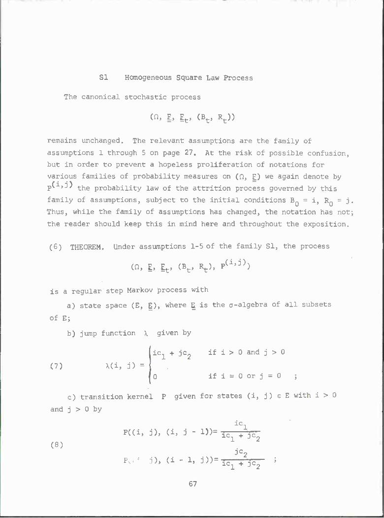
SI Homogeneous Square Law Process
The canonical stochastic process
(n, E, Et, (Bt, Rt»
remains unchanged. The relevant assumptions are the family of
assumptions 1 through 5 on page 27. At the risk of possible confusion,
but in order to prevent a hopeless proliferation of notations for
various families of probability measures on (fl, F) we again denote by
pQ1»^; the probability law of the attrition process governed by this
family of assumptions, subject to the initial conditions BQ = i, RQ = j.
Thus, while the family of assumptions has changed, the notation has not;
the reader should keep this in mind here and throughout the exposition.
(6) THEOREM. Under assumptions 1-5 of the family SI, the process
(n, E, Et, (Bt, Rt), P(l,3))
is a regular step Markov process with
a) state space (E, §), where E. is the o-algebra of all subsets
of E;
b) jump function \ given by
(7) X(i, j) =
ic. + jc2 if i > 0 and j > 0
0 if i = 0 or j = 0 ;
c) transition kernel P given for states (i, j) e E with i > 0
and j > 0 by
icn P((i, J), (i, J - D)=
(8) 1C1 + JC2
Z)C2 P,.< j), (i - 1, J))=ic + je,
67

d) infinitesimal generator Q given for states (i, j) with
i > 0 and j > 0 by
Q((i, J), (i, j - 1)) = ±c1
(9) Q((i, j), (i, j)) = - (icx + jc2)
Q((i, j), (i - 1, j)) = jc2 .
If i = 0 or j = 0, Q((i, j), x) = 0 for all x e E.
PROOF. Let EQ = |(i, j) : i > 0, j > 0}. Since there clearly is no
further attrition once one side is annihilated, every state in E - En is absorbing. Also, with probability one the state (0, 0) is never
entered unless the process begins there.
We begin by showing that if (i, j) e E~ and t > 0, then
PCl'J)i(Bu, Ru) = (i, j) for all u e TO, tl|
= P(i'j)|(Bt, Rt) = (i, j)}
= exp [ - (ic1 + jc2)tl .
Let V denote the time at which the process first changes state,
which in this case is also the first time at which a fatal shot is
fired. We are trying to compute p^'^'jv > t}.
Fix attention on a particular Blue combatant, say the k one and
consider the times BSQ
a 0, _S^k \ R2 ' •" at wnicn ne would
fire shots if he survived and continued firing forever. By assumptions
2) and 3) the sequence ( S^ ') Q is a simple Poisson process with
rate r . Suppose in addition tfhat all shots fired by all combatants
have only "hypothetical" effects in the sense that no combatants are
killed but a record is kept of shots which would have been fatal with-
out this restriction. This converts the attrition process into a non-
terminating process in which each combatant continues firing shots
68

forever, some of which cause "hypothetical" kills of opponents. The
hypothetical process not only has nicer behavior than the
original attrition process but also serves to describe the attri-
tion process because of the following two properties:
(a) The time of the first hypothetical kill is the time at which
the attrition process first changes state;
(b) The side suffering the first hypothetical casualty also suffers
the first casualty in the attrition process.
Thus consideration of the process of hypothetical kills suffices
by (a) to compute the jump function of the attrition process and by
(b) to compute its transition kernel, as well as by (a) and (b)
together to establish the Markov property. Computations involving
the process of hypothetical kills are easy to do, so we shall use
throughout the approach of considering processes of hypothetical kills.
By the Random Sampling Theorem for Poisson processes, the (k^ th times (-S^ ') n of hypothetically fatal shots fired by the k Blue B n n>u
combatant fornPa Poisson process with rate c, = r p. .
Similarly, for each i , the set (DS^O of times of hypothetically
fatal shots fired by the I Red combatant is a simple Poisson process with rate c„.
By assumption 5) the random variables S^ , ..., RS^1^
„Si; ' , ..., TJS!| ' are mutually independent with respect to P^ '-'•',
Furthermore V > t if and only if S:; ' > t for k = 1, ..., i and
CCJD RJ > t for I = 1, ..., j, since
V = min<S(1) S(i) S(1) S(jH
69

Therefore
P^'^IV > t} = P(i'J){B4k) > t, k = 1, ..., i; RS^> > t, £ = 1, ..., j}
= I" n pCi'j)lBs^k) > tfl I" n P^^S^ > tfl
■ Li •Ti, •""] " = exp [ - (icx + jc2)t] .
The same reasoning and Memoryless" properties of the exponential
distribution apply to show that for each t and s
P(ls:i)|(Bu, Ru) = (Bs, Rs) for all u e [s, s + t]||s|
= exp [ - (c-jBg + c2Rg)t] .
This proves that the process ((B., Rt)) has jump function \ defined
in ( 7) above.
We next show that for (i, j) e EQ,
p(i'J)KBv+> *W = Ci- l, J)} =TZ-TTc
and
PCi'J)iCBv+J Rv+) = (i, 3 - 1)1=15^3
where
is the state entered by the process at the time V of the first
fatality. It seems plausible that that state must be either
(i - 1, j), if the first fatality is suffered by Blue, or (i, j - 1),
if the first fatality is suffered by Red.
70

I
Let
and
Then
and
SB=nlnlBSi1)» — • B8!^}
8RrdBtfll>. — • RSiJ)} '
pCiJ)iCBv+, V-) = (i " x' j)* = P(i,j)W = sRf
= p(i>^{sB > SR|
p(i,J)i(Bv+» Rv+) = (i» j * X)J = p(i,j)iv = S
B1 = p(i>j))sB<sR| .
Since Sß is exponentially distributed with parameter ic. and S„ is
exponentially distributed with parameter jc« and S~, Sp are independent
(all these assertions hold with respect to the probability measure
p'1»-3', of course), it follows that
p(i'j){sB = SR\ = 0
and therefore
P(i,J){(Bv+, Rv+) ef(i - 1, j), (i, j - 1)}} = 1 .
We next compute that
P(i'J){SR < SB} = E^'^CP^'^jSj^ < SB|SR|]
= jc2 J exp ( - jc2v) exp ( - i^v) dv 0
ic1 + jc2 »
71

where E^ »■'' denotes expectation with respect to the probability P^1'^,
Similarly,
,<i,J)lsB<sRl=i; 1C.
1 + 1C2
For each t let Vt denote the time of the first fatal shot fired
after time t . Then again using the "memoryless" property of the
exponential distribution, one obtains
,(i,j)
(Bt,Rt)
K,+' v} = (k' £)||tf t t
= P K+' v* = (k> l)\ = P((Bt, Rt), (k, £)),
where P is defined by (8), for each t and (k, £).
Hence ((B , R+-))t^n nas tne Markov property, the given jump
function, and the given transition kernel. That this process then
has the infinitesimal generator Q. given in (9) follows from the
theory of regular step processes, cf p. 57.
Here are some additional properties of this process which are of
physical interest.
COROLLARY. The following properties hold.
1) With probability one, the functions t -» B. and t -♦ R. are nondecreasing;
2) If i / 0, j / 0, then
P^1,:^{(Bt, Rt) = (0, 0) for some t} = 0 .
Property 1) certainly makes sense: if there are no reinforce-
ments, surviving force strengths can only decrease. The second
assertion, which is true even if c, = c„ and initial force strengths
are numerically equal, states the "mutual annihilation at time t = »n
which occurs in the deterministic Lanchester square model is almost
surely impossible in this model.
70

-WVT
We wish to emphasize that although the vector process ((B , R1-))t^n
is a Markov process, neither of the individual survivor processes
(Bt^t>0 and (R^^n is Markovian, at least with respect to the family of
histories (Et)t>0~. If t is fixed, then the history |t contains
information other than the current state B which is helpful in
predicting the future course of the process (B ); that is, in
predicting (Bg) t. That information is, of course, the current
number R of Red~survivors. (It couldn't be anything else, for
otherwise ((B , R )) wouldn't have the Markov property.)
This model can be extended to allow for reinforcements which arrive
in a particular manner, namely, according to compound Poisson processes,
as we now indicate.
Feller (1966) contains sufficient background. For our purposes
a compound Poisson process is defined by a positive number a and
a probability distribution cp on N* = {1, 2, ...}. Let TQ = 0,
T,, T9, ... be the times of arrivals of a simple Poisson process
with rate a and let X,, X2, ... be independent and identically
distributed as cp . Assume that (T ) and (Xk) are independent and
define
N = Z X , t > 0 . n:T <t n—
One interprets (N.) is an arrival counting process; that is, Nt is
the number of objects which have arrived up until time t . At each
of the times T,, T9, ... a random number of objects arrives, which is
distributed as cp .
Consider now the following additional assumptions.
6. Reinforcements to the Blue side arrive according to a compound
Poisson process with parameters (a-,> cp-,). Reinforcements to the Red
side arrive according to a compound Poisson process with parameters
(a2> cp2). All reinforcements immediately enter the combat.
73

7. The two reinforcement processes are independent of each other
and of all firing processes.
For (i,j) e E, let p^1»^ denote the probability law of the homo-
geneous square law process with reinforcements, governed by assumptions
1-7 above and conditioned on the event { (Bn, Rn) = (i, j)|.
(10) THEOREM. The process
(n, E, Et, (Bt, Rt), P(i>j))
is a regular step process with
a) state space (E, E) as defined for Theorem (6);
b) jump function X given
IiCl + ^C2 + al + a2 if i > 0 and j > 0
{a^ + a2 if i = 0 or j = 0 ;
c) transition kernel P given for states (i, j) with i > 0 and
j > 0 by
icl P((i, j); (i, J - D) = ic . ,c . n . „ lc-i + jc_ + a-i + In
P((i, j); (i - i, d)) = iCi + jc*+ tti + ag
(12a) o
p«i, »: (i + k, j)) -^(k) iCi t jC; I Bi ^ a
P((i, j); (i, j ♦ i» =V2(i)l__n_^__
and for states (i, j) with i = 0 or j = 0 by
P((i, J); (i + K j)) = cp,(k) ^— , k > 1 (12b) x *
P((i, j); (i, J + £)) = cp9U) 1—- , I > 1 ; * a-j_ + a2
74
2
5
2
k > 1
£ > 1
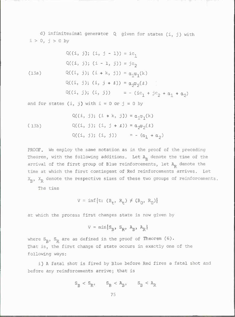
d) infinitesimal generator Q given for states (i, j) with
i > 0, j > 0 by
(13a)
Q((i, j)
Q((i, j)
Q((i, 3)
Q((i, 3)
Q((i, j)
(i, j - 1)) = iC;L
(i - 1, j)) = jc2
(i + k, j)) = a^Ck)
(i, j + i)) = a2cp2(X)
(i, j)) - (ic-L + jc2 + ax + a2)
and for states (i, j) with i = 0 or j = 0 by
(13b)
Q((i, j); (i + k, j)) = axcpx(k)
Q((i, j); (i, j + £)) = a^p2(l)
Q((i, j); (i, j)) = - (ax + a2)
PROOF. We employ the same notation as in the proof of the preceding
Theorem, with the following additions. Let A_ denote the time of the
arrival of the first group of Blue reinforcements, let A~ denote the
time at which the first contingent of Red reinforcements arrives. Let
X^, Xp denote the respective sizes of these two groups of reinforcements,
The time
V = inf{t: (Bt, Rfc) ? (BQ, RQ)}
at which the process first changes state is now given by
V = minjSB, SR, AB, A^
where SR, SR are as defined in the proof of Theorem (6).
That is, the first change of state occurs in exactly one of the
following ways:
i) A fatal shot is fired by Blue before Red fires a fatal shot and
before any reinforcements arrive; that is
Sr> < Sp, S_ < A_, 'B B B: SB<AR
75

ii) Red fires a fatal shot before Blue does and before any
reinforcements arrive:
SR < SB' SR < V SR < AR iii) Some Blue reinforcements arrive before any Red reinforcements
do and before any fatal shots are fired:
AB < V AB < SR' AB < AR
.v) Some Red reinforcements arrive before the arrival of any Blue
reinforcements and before any fatalities:
\ < SB' AR < SR' AR < AB •
By assumptions 2, 3, 4, 5, 6, and 7, the random variables SR, SR,
A„, AD are independent and exponentially distributed with means 1/ic , B R -L 1/jc , 1/a-, and l/a?, respectively. Therefore V is exponentially
distributed with mean l/(ic + jc + a-, + do) = Uijj); in other words
( 14) P(l>3}|(BU, Ru) = (i, j)forO<u<t}= exp[ - \(±, j)t]
for all (i, j) and t , where \ is given by (11).
Moreover, since
p(i'J)iSB = SR °r SB = AB °r SB = AR °r SR = AB °r SR = AR °r AB = AR ^ = °
it follows that
P(i'")(Bv+, R^) . Ei>d( = 1
where
E±j = |(i - 1, j), (i, j - 1)|U {(k, j): k > i}
U 'j (i, I): i > j\.
That is, two or more simultaneous fatalities (on either the same or
opposite sides) or a simultaneous fatality and arrival of reinforcements,
fail to occur almost surely.
76

Proceeding as in the proof of Theorem (6) we see that
P(i'j)j(Bv+, Rv+) = (i, j - l)f
=P(i>j)|sB<SR, SB<AB, SB< AR}
iCl iCl + ^°2 + al + a2 '
that
P(i>j){(Bv+, Rv+) = (i - 1, j)}
= P(i'J)|SR< SB, SR<AB, SR<AR[
:2 icl + 3°2 + al + a2 '
that
jX±,J)((Bv+» RV+) Gl(k> j): k> ^
= p(i'J)K<SB' AB<SR> AB<A
RI
'1 ic1 + 3C2 + a1 + a2
and, finally, that
P ' KBV+'
RV+) ei(i' £): l > j^
=p(i'J)lAR<SB' AR<SR' AR<AB} a o
" ici + ^c2 + ai + a2 '
Let us consider the latter two expressions in more detail. Since
(B„ , R.. ) = (k + i, j) with k > 0 if and only if the first event
causing a change of state is the arrival of a group of Blue reinforcements
77

which number exactly k, we have
p(i'J)iCBv+> V5 = (i + k' j)(
= p(i'J)lÄB<SB' AB<SR> h< V h = ^ •
By properties of the compound Poisson process of Blue reinforcements
and assumption 7, 2L. is, with respect to the probability V^1,-i ,
independent of A_, S„, S„, and A,,, and therefore
P(i'^iAB<SB, AB<SR5 AB<SR, X^k}
(15a) = P^»^)^ < sB, AB < SR, AB < SR| P^'^iXj, = k}
±c± + jc2 + a + a2 ^l' ' *
Through entirely analogous reasoning we are able to obtain
p(i'J)i(Bv+' Rv+) = (i' j + ^
(15b) a2 , A cp9(k) 1 1 + J 2 + al a2
for each i > 0.
We may, on the basis of (12), summarize (15) in the form
(16) P(i'j){(Bv+, Rv+) = (k, l)\ = P((i,j), (k, I))
for all (i, j), (k, I) e E.
78

Using standard arguments concerning the exponential distribution,
one extends (14) to
P(i';])|(Bu> Ru) = (Bs, Rs) for s < u < s + t||8|
= exp T - X(Bs, Rs)t]
and (16) to
P(1>j){(Bv+, Rv+) = (k, £)|ES| s s
= P((BS, Rs); (k, £)),
where
\7s = infju > s: (Bu, Ru) * (Bs, Rg)}
is the time of the first change of state of the process after time t.
These last two statements combine to complete the proof of the
Theorem.
Note that the process with reinforcements has no absorbing
states.
Other types of assumptions concerning reinforcements are possible,
but would be more difficult to handle and are almost certain to destroy
the Markovian property of the process, although if the resultant model
were a semi-Markov process it might still be tractable.
79

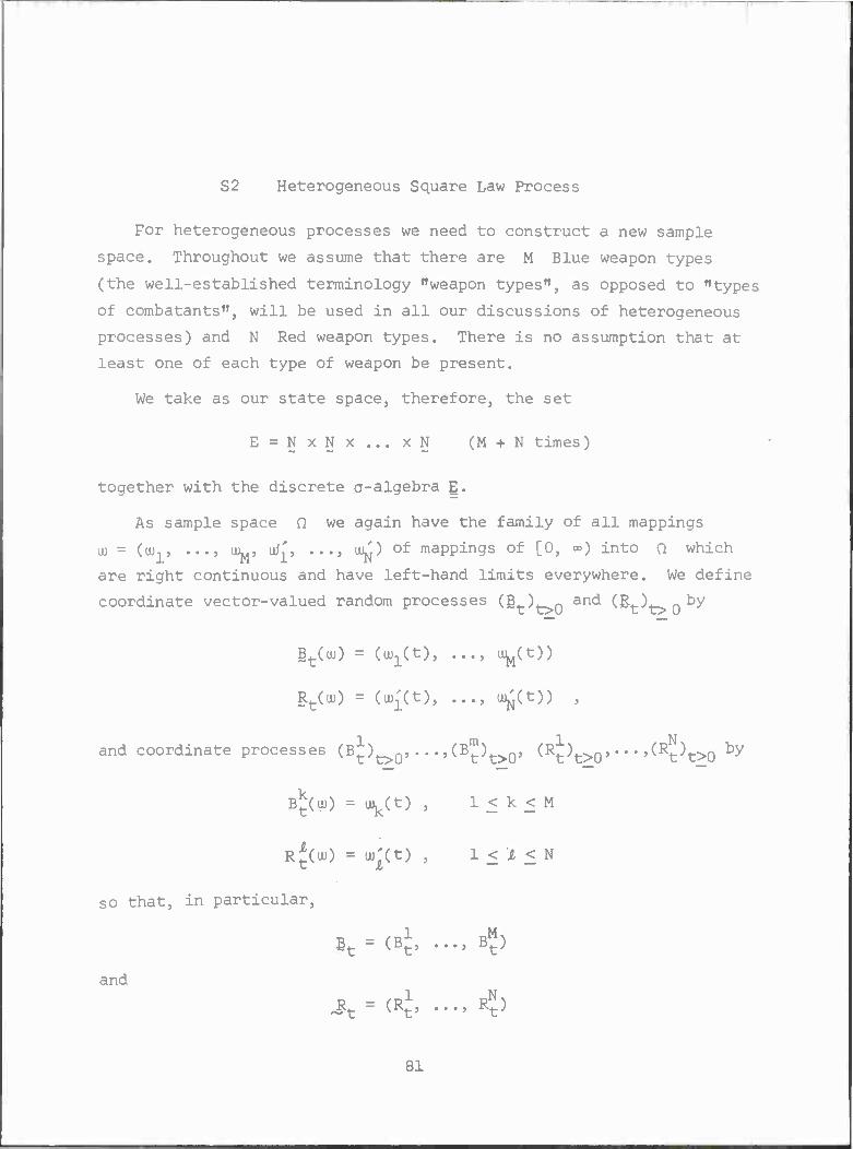
S2 Heterogeneous Square Law Process
For heterogeneous processes we need to construct a new sample
space. Throughout we assume that there are M Blue weapon types
(the well-established terminology "weapon types", as opposed to "types
of combatants", will be used in all our discussions of heterogeneous
processes) and N Red weapon types. There is no assumption that at
least one of each type of weapon be present.
We take as our state space, therefore, the set
E=NxNx...xN (M+N times)
together with the discrete o-algebra E.
As sample space Q we again have the family of all mappings
uu = (ujp ..., uujj, uip ..., iDjJ) of mappings of [0, ») into Q which
are right continuous and have left-hand limits everywhere. We define
coordinate vector-valued random processes (g ) and (R ) by
§t(w) = (uu^t), ..., a^(t))
Rt(u0 = (u)£(t), ..., uu^(t)) ,
and coordinate processes (Bt)t>0» " ''^Bt^t>0} ^Rt^t>0' " ''^Rt^t>0 by
,k, B £<«») = «^(t) > 1 < k < M
R*(w) = w't(t) , 1 < I < N
so that, in particular,
Bt = (Bt> •••> Bt^
and
,Rt = (R^-5 • • • J R^-)
81

for each t . B. is the number of Blue type k weapons surviving at
time t, B. the Blue force surviving at time t, R* the number of type l
Red weapons surviving at time t, and R. the surviving Red force at
time t.
As before, we put
Et = a|(Bs, Rs): 0 < s < t}
and
E = a|(Bs, RJ: s > 0\ .
F is the history of the attrition process up until time t and F its
entire history
We denote points in E in the form (x,y) where x e N and y e N ;
x thus is a state which the vector of Blue surviving weapons may
assume and similarly for y and Red. x. corresponds to surviving
Blue type i weapons and y. to surviving Red type j weapons.
For each (x,y) e E, let P^ '^' denote the probability law on
(0, E) °f the attrition process governed by assumptions 1-6 of the
Process S2, when (Bg, RQ) = (x, y).
(17) THEOREM. Under the S2 assumptions,
(n, E, Et, (Bt, Rt), P(x'^)
is a regular step process with
a) state space (E, |) as defined above;
b) jump function \ given by
i:x.>0 j:y.>0 [c2(i,j)y + c1(j,i)xi] if x jt 0, y / 0
82,
if x = 0 or y = 0;

c) transition kernel P defined for states (x,y) with x / 0 and
y ^ 0 by
M £ c1(j,i)xi
P((x,y); (x;y1L...,y^-l,...,yN)) = X~\(x y)
for j = 1, ..., N such that y. > 0 and by
N E c2(i,j)y.
P((x,y); (x1,...,x1-l,...,^!;y)) = 3=1
x(X}y)
for all i with 1 < i < M and x. > 0;
d) infinitesimal generator Q given for states (x,y) with x ^ 0
and y ^ 0 by
M IE c (j,i)x. if y > 0 i=l x x 3
0 if y. = 0
Q((x,y);(x,y)) £ E [c (i,j)y + c (j,i)x,] i:X;.>0 j:y.>0 * 3
N
Q((x,y);.(x1,...,xi-l,...,xM;y)) =
E c2(i,j)y. if x. > 0 |i=l J
0 if x. = 0
and for states (x,y) with x = 0 or y = 0 by Q((x,y); Q) = 0 for all
C e E.
83

PROOF. We recall that for q = 1,2 and appropriate k,£ we have defined
cq(k,£) = rq(k,£)pq(k,jO .
For i = 1, ..., M let
SR(i) = inf{t: B£ 7* BQ}
be the time at which the first fatality to a Blue type i weapon occurs.
If there is no such time, and in particular if BQ = 0, we put S~(i) = + ».
Similarly, let
SB(j) = inf jt: R3tji R3
Q\ , j = 1, ..., N
be the time of the first fatality, if there is one, to a Red type j
weapon.
We claim that
P(X'y)|SR(i) > t, i = 1, ..., M, SB(j) > t, j = 1, ..., N}
(18)
= exp ( - t E S [c2(i,j)y. + c1(j,i)xi]) i:x.>0 j:y->0 J
from which it follows that, if we define
V = infjt: (Bt, Rt) ? (B0, R0)|
then since
V = minjSB(l), ..., Sß(N), SR(1), ..., SR(M)} ,
one has
p(x,y)|v > t} = exp [ - X(x,y)t] .
84-

Now, how are we to prove (18)? If all kills were hypothetical
only, then for a given j and i , the times of "hypothetical" kills
of type j Red weapons by type i Blue weapons would, by assumptions 2
and 4 form a Poisson process with rate c.(j,i)x., so long as y. > 0.
Hence by hypothesis 6, "kills" of type j Red weapons occur hypothetically
at the arrival times of a Poisson process with rate
E c1(j,i)xi ;
in particular the time S£(j) of the first such hypothetical kill is
exponentially distributed with mean ( £ c.(j,i)x.)~ if y. > 0 and i x 1 3
mean + » if y. = 0. Moreover, by hypothesis 3, S£(l), ..., S*(N) are -J x v)
independent with respect to Pv ,J.
If S£(i) similarly stands for the time of the first hypothetical
kill of a Blue type i weapon, then S*(i) is exponentially distributed,
with respect to the probability P^x' , with mean
((S c2(i,j)yj)"1 if Xi > 0
+~ if x. = 0 .
Assumption 3 assures us that s£(l), ..., S&(M) are independent and
assumption 6 implies that |S*(1), ..., S*(N)| and Js|?(l), ..., S*(M)(
are independent.
Furthermore, even though by definition
V = minjSB(l), ..., SB(N), SR(1), ..., SR(M)f
it is also true that
V = minjS*(l), ..., S*(N), S*(l), ..., S*(M)}
since the times of the first actual and hypothetical kills necessarily
coincide. 85

Thus
p(x,y){v > tj - p^x'y){S*(l) > t, ..., S*(N) > t ,
S*(l) > t, ..., S*(M) > t(
= P(x'y)|s*(l) > t( ... P(X'y){S*(N) > tf
x P(x>y)|s*(l) > tf ... P(X'y)|s*(M) > tf
= exp [ - t s E c.(j,i)x.] j:y-j>0 i
x exp C - t E E c (i,j)y ] i:x±>0 j J
which completes the proof of (18).
We note that if j ^ &, i ^ k
p(x,y) |s*(j) _ S*U)) s*(j) < 00> s*u) < „j = 0
and
P(x,y) |s*(i) = s*(k)j s*(i) < », s*(i) < »I = o
and that
P(x,y) |s*(j) = s*(i)j s*(j) < 00} s*(i) < .[= o
for all i,j, by independence and exponential distributions of the
random variables involved..
Since
p(X'y)i(§V+' ?V+) = (X;yl' •' yj"lj ••" yN^
= P(X'y){S*(j) < S*(£), I ? j; S*(j) < S*(i) for all i}
86

it follows that
P ' j(~V+> P>V+^ eKw>z): wi = xi_1 for exactly one i and
otherwise w = x and z = y or z. = y.-l for
exactly one j and otherwise, z = y and w = x}
Again by independence and exponential distributions
p(x,y) |s*(j) < s*U)j £ ^ j; sg(j) < s*(i) fQr all .j
if y. = 0 J
E c1(j,i)xi i if y. > 0
= 1.
S E c.(j,i)x. + E E c1(i,j)x. 3
jry^O i A irx^O j
and similarly,
PCx'y)i(§v+> hJ = (xi' ••" V1' •••' V y)f
= P(x'y) |s*(i) < S*(k), k *L; S*(i) < S*(j) for all j}
if x. = 0 l
E c2(i,j)y.
if x. > 0 . E E c (j,i)x. + E E c (i,j)y.
j:yj>0 i x irx^O j J
Hence we have shown that
p(x'y) K?v+» 5v+> = sf = p<<x>y>; ?)
for all § e E, where P is the transition kernel defined in the
statement of the Theorem.
87


' ■'" 'T '
S3a Heterogeneous Square Law Process
We continue to assume that there are M Blue weapon types and
N Red weapon types, and that the canonical stochastic process
CO, E, Et, (Bt, Rt))
is as described in the preceding section. P^ '*' will now denote the
probability law of the attrition process governed by the family of
five assumptions for the Process S3a, subject to the initial conditions
50 = y« f ■
(19) THEOREM. Under the assumptions of Process S3a, the collection
(n, E, Et, (Bt, Rt), P(x>y>)
is a regular step process with
a) state space (E, E) as defined in the description of Process S2;
b) jump function \ given by
M N
j E _E [x p (i,j)r9(j)y. + y.p,(j,i)r1(i)x.] if x ^ 0, y ? 0 i=l j=l
X(x,y) =
if x = 0 or y = 0
where M
x. = x./ E x, , i = 1, ..., M 1 1 k=l K
and N
yn. = yJX yt , j = l, ..., N ; 89

these quantities are defined only if the denominator is positive;
c) transition kernel P given for states (x,y) e E such that
x ^ 0 and y jt 0 by
P((x,y); (x;y1} ..., y_. - 1, ..., yN))
M E P1(j,i)r1(i)xi
~ i=l . _ . Vj X(x,y) ' " X' '••' N
P((x,y): (x15 ..., xi-l, ..., xM;y))
N E P2(i, j)r2(j )y^
= *i J=1 X(x,y) > i = l, ..., M;
d) infinitesimal generator Q given for states (x,y) with x ^ 0
and y / 0 by
Q((x,y), (x;y19 ..., y^-1, ..., yN)) = y^ Z p1(j,i)r1(i)xi
M N Q((x,y), (x,y)) = - S S [x.p2(i,j)r2(j)y. + y •P1(j,i)r1(i)x;L]
i=l j=l J
N Q((x,y);(x1, ..., xi-l, ..., x^y)) = x± S P2(i} j )r2(j )yj .
If x = 0 or y = 0, Q((x,y), a) = 0 for all a e E.
PROOF. As usual consider the hypothetical situation in which no
weapons are actually killed, but only "potential" kills are recorded,
in terms of the times at which they occur. Following the notation of
the preceding proof we let S*(j) denote the time of the first hypo-
thetical kill of a Red type j weapon, j = 1, ..., N and for i = 1,
.... M we denote by S$(i) the time at which the first hypothetical
kill occurs of a Blue type i weapon. Then the time
90

V* = min|S*(l), ..., S*(N), S*(l), .,., S*(M)f
of the first hypothetical kill coincides with the time
V = inf{t: (Bt, Rt) ^ (BQ, RQ)}
of the first actual kill, which is also the time at which the attrition
process first changes state.
For i = 1, ..., M and j = 1, ..., N let K|(i,j) be the time of the
first hypothetical shot which is fatal to a Blue type i weapon and was
fired by a Red type j weapon. Similarly, let K*(j,i) be the first
time at which a Red type j weapon is hypothetically killed by a Blue
type i weapon. Then
S*(i) = min{K*(i,l), ..., K*(i,N)f
and
S*(j) = min{K*(j,l), ..., K*(j,M)|
for all appropriate i and j .
Consider now a fixed Blue weapon of type i. The times of hypo-
thetical shots which it fires form a Poisson process with rate r,(i).
Further, by assumption 3
pQX>y;|a hypothetical shot fired by a Blue type i weapon
is directed at some Red weapon of type j}
(20) _ N
= yH = yJ z y. ; 3 3 l=1 I
this is also the probability that an actual shot fired at a Red force
of composition y is directed at a target of type j. A similar ex-
pression holds for shots and hypothetical shots fired by Red weapons.
Hence hypothetical shots fired by a particular Blue type i which are
directed at Red weapons of type j form a Poisson process with rate r,(i)y.
91

with respect, of course, to the probability P^ ' , which is assumed
fixed for the purposes of this discussion. The fatal shots fired by
this weapon at Red type j weapons thus constitute a Poisson process
with rate r (i)y.p (j,i). By assumption 6, therefore, hypothetically
fatal shots fired at Red type j weapons by all type i Blue weapons
form a Poisson process with rate x^r (i)y.p (j,i).
Another application of assumption 6 shows that the times of all
hypothetically fatal shots fired at Red type j weapons form a Poisson
process with rate
E x±r (i)y.p (j,i) i J
and therefore
(21) P(X'y){s*(j) > t| = exp[ - ty\ E P^j,!)^!^] .
Similarly, since
P(X,y)|K*(i,j) > t( = exp[ - txip2(i,j)r2(j)yj]
for each i and j yet another application of the independence
assumption 6 yields
(22) P(x'y)|s*(i) > t( = exp[ - tx E P2(i, j )r2( j )y, ] . j
From these two expressions
P(x,y)jv* > t\ = exp[ - \(x,y)t]
92

(23)
follows and hence
P(x,y)|v > t| = exp[ _ x(x>y)t] #
Proceeding exactly as in the proof of Theorem (17) we see that
P(X'y){CBv+, 8y+) = (x;yi, ..., y.,-1, ..., yN)f
= p(x'y){v* = S*(j)f
= P(X'y)|s*(j) < S*U) for i jt j, S*(j) < S*(i) for all i
y\j T. p1(j,i)r1(i)xi
and, analogously, that
P(X'y)|(Bv+, Rv+) = (xx, ..., x.-l, ..., x^y)}
= p<x,y)jv* = s*(i)}
= P(x'y)jS*(i) < S*(k) for k ^ i, S*(i) < S*(j) for all j}
(24)
xi S P2(i>j)r2(j)y. j :
X(x,y) D
93


S3 Heterogeneous Square Law Process
The notation is exactly that of the previous two processes.
P*- >y) now denotes the probability law of the attrition process
governed by the family of assumptions of Process S3, subject to the
initial conditions (BQ, RQ) = (x,y).
(25) THEOREM. Under the assumptions for Process S3, the collection
cn» I» It» (Bt, Rt), p(x»y))
is a regular step process with
a) state space (E, E) as defined above;
b) jump function X given by
M N X(x,y) = E S [YiCy.D^PiCJ.Dr.CDx. + n.(x,i)p2(i,j)r«(j)y.]
i=l j=l x x i : z ' 3
(we assume that y. = 0 implies ¥i(y,j) = 0 for all i);
c) transition kernel P given for states (x,y) with x / 0 and
y ± 0 by
M S Yi(y,j)p1(j,i)r1(i)xi
P((x,y);(x;y1, ..., y^-1, ..., yN)) = -=1 \(x,y)
S T]j(x,i)p2(i,j)r2(j)y:.
P((x,y);(x1, ..., x±-l, ..., ^y)) =2 X(x,y) ;
d) infinitesimal generator Q given for states (x,y) with x ^ 0
and y / 0 by
M Q((x,y);(x;y1, ..., y.-l, ..., yN)) = E Yi(y,j)P1(j,i)r1(i)x1
95

M N Q((x,y);(x,y)) = - E E [Y,(y,j)p,(j,i)r1(i)x. +
i=l j=l x x 1
+ tij(x,i)p2(i,j)r2(j)yj]
N Q((x,y);(x1, ..., x.-l, ..., x^y)) = E Ti;j(x,i)p2(i,j)r2(j)y
If x = 0 or y = 0, Q((x,y),a) = 0 for all a e E.
PROOF. The proof of Theorem (19) requires only notational changes.
By the new assumption 3, (20) becomes
(20*) p(x»y) | A hypothetical shot fired by a Blue type i weapon
is directed at some Red weapon of type j }
= Y±(y,j)
so that hypothetical shots fired by a given Blue type i weapon at
Red type j weapons form a Poisson process with rate r (i)y.(y,j)
and hypothetical fatal shots fired by this type i weapon at
Red type j weapons form a Poisson process with rate
r, (i)Y-,(y, j )P-i(J,i)> in which case for (21) one obtains
(21*) P(X'y) |s*(j) > t| B'
exp[ - t E Yi(y,j)P1(j,i)r1(i)xi] ; l
analogously, (22) becomes
(22*) p<x>y> |S*(i) > t}
= exp [- t E Ti.(x,i)p2(i,j)r2(j)y.] . j J
96

In the same manner one obtains as analogs of (23) and (24) the
following:
(23*) P(x'y){s*(j) < S*U) for l * j, s*(j) < S* (i) for all i|
S Yi(y,j)p1(j,i)r1(i)xi
= xTxTy5
for j = 1, ..., N and
(24*) P(x>y>|s*(i) < S*(k) for k * i, S*(i) < S*(j) for all jf
E Ti.(x,i)p2(i,j)r2(j)y. j J 1
respectively.
The Theorem now follows. II
EXAMPLES. The fire allocation scheme of this process is quite
general, but also entirely abstract. Here are three specific cases,
1. Uniform Fire Allocation occurs when
N Y4(y»j) = y.; = yj s y
and
cp.(x,i) = x. = x./ E x,^ 3 a x k=l K
1 £=1 £
M
for all i and j and in this case the Process S3 reduces to the
process S3a. It becomes clear, therefore, that Process S3a is a
Lanchester square process.
2. Priority Fire Allocation can occur in the following manner.
Consider a fixed type of Blue weapon, say type i, and suppose that
97.

the Red weapon type 1, ..., N are ranked in some order j ..., j
(here {j , ..., j f is simply a permutation of the set jl, ..., N|)
in such a manner that a Red weapon of type j will never be fired
upon when a weapon of type j is present. One models this by Jw — -L
putting
YiCyJjj*) = i
where
I* = infjjJ: y. > 0} .
Other more flexible and possibly more realistic priority schemes can
certainly be developed.
3. One may also derive fire allocations from physically meaningful
axioms. For example, consider the following hypotheses on the family
JY.}of fire allocation distributions
i) Y-(yjj) = 0 if and only if y. = 0;
ii) For all y and z
N y vAy + z,J) = Y,(y,j) E E v i z Yi(y + z)U)]
N z + ¥.(z,j) [ E I Y,(y + z)(£)]
for all j = 1, ..., N.
The interpretations of all these assumptions are physicallly
meaningful. The first states that a weapon type not present
receives no fire but that every weapon type present receives
98

a positive fraction of the fire. The second hypothesis is best
explained step-by-step. Consider the effect of combining two
target forces y and z into the single force w = y + z.
Y.(y + z, £) is the proportion of fire directed at the combined
force w which is allocated to type I weapons. If this is
further allocated among the type I weapons from the two com-
ponent forces (y and z) in proportion to the relative numbers
of such weapons present then
*r*V<y + z> ° is the fraction of fire directed at the combined force that is allo-
cated to type i weapons originally part of the y-force. Thus
N y ay = E y + z Y <y + z> *> y £=1 yi I
is the proportion of fire allocated to weapons of types originally
and the y-force and
*z= ,". yTTT:" (y + z> l)
the fire allocated to weapons originally in the z-force. But the
fire represented by a should be allocated among weapon types
according to the distribution ¥ (y, •) and similarly for a so that z one should have
Y (y + z, •) = ayY (y, •) + a/ (z, •)
which is exactly the second assumption. If an assumption like this
did not hold, consistency problems would arise, with fire allocation
dependent on names given targets rather than only numbers of targets.
99

(For example, arbitrarily splitting a class of n indistinguishable
weapons into two subclasses of n "Type A" and n - n, "Type B"
weapons would change the fire allocation).
We have conjectured, and J. Blankenship (1973) has proved, using
the notion of invariant measures for Markov matrices, that any family
| Y | of allocation distributions satisfying i), ii), iii) above is
necessarily of the form
a.y. f(y,j) = N
J 3
£=1 l l
where
3j = *(l,j) , j = 1, ..., N
and 1 = (1, ..., 1). It is possible, moreover, to express the Y
and terms of Y (y, *) for any fixed y such that y. > 0 for all j.
Thus if one accepts the hypotheses i), ii), iii) then the fire alloca-
tion for every target force can be computed from that for a "base"
force.
We remark in conclusion that even if different weapons may employ
qualitatively different means of allocations, the model remains valid.
100

LI Homogeneous Linear Law Process
We return to the sample space and canonical stochastic process
previously established for the homogeneous case. Thus, the state
space is
E = N x N
together with the discrete a-algebra £, Q is the set of mappings
ID = (CD, , u)2) from [0, co) into E which are right-continuous with
left-hand limits everywhere,
Bt(u») = u^Ct) e E
Rt(üü) = uu2(t) e E
for each t > 0,
it = a((Bu' V : ° < u< t)
is the history of the attrition process up until time t and
F = a((Bu, Ru) : u > 0)
the entire history.
From each (i,j) e E we denote.by P11»3', as usual, the probability of
the attrition process conditioned on the event |(BQ, RQ) = (i,j)f
and this time governed by the five assumptions listed in the main
text for the Process LI..
(26) THEOREM. Under the assumptions of Process LI, the collection
(0, E, Et, (Bt, Rt), P(i'j))
101

is a regular step process with 2
a) state space E = N ;
b) jump function \ given by
X(i,j) = iJC^ + k2);
c) transition kernel P given for states (i,j) with i > 0 and
j > 0 by
kl P((i,j), (i,j - D)= k +\
k ' P((i,j), (i - l,j)) = k /k ;
d) infinitesimal generator Q given by
Q((i,j), (i,j - D) = kxij
Q((i,j), (i,j)) = - (k-L + k2)ij
Q((i,j), (i - 1, j)) = k2ij .
We remind that for £ = 1, 2
k„ = s„q.
where 1/s, is the mean time required for a particular Blue weapon to
detect a particular Red weapon and q, the conditional probability that
a Blue weapon destroys a Red weapon (in a one-on-one engagement, the
only sort of engagement permitted in this model, which is also assumed
to occur instantaneously) given detection and attack, s» and q are
analogous descriptions of Red weapons.
PROOF. We again use the device of hypothetical kills, which is
useful because it preserves independence and stationarity properties
which are not valid for the actual attrition process, yet allows us
to make statements about the actual process because the time of the
first hypothetical kill is also the time of the first actual kill
102

(namely, the first time at which the attrition process changes state)
and the weapon killed at the first hypothetical kill is also the first
weapon actually killed. Thereafter the two processes diverge from
one other and the hypothetical process is no longer a useful means
of dealing with the actual process.
We therefore denote by T*(k,jO the time at which the k Blue
weapon (first) hypothetically detects and kills the J Red weapon
(not every detection results in a kill unless q, = 1) and let . ■t~Vi
T£(jfc,k) be the time at which the i Red weapon first hypothetically th kills the k Blue weapon.' Then according to assumptions 2, 3, 4, 5
and the Random Sampling Theorem for Poisson processes, the random
variables T*(l,l), T*(l,2), ..., T*(l,j), T*(2,l), T*(2,2), ...,
T*(2,j), ..., T*(i,l), T*(i,2), ..., T*(i,j) are independent and
identically exponentially distributed with mean 1A-.» Symmetrically,
T*(l,l), ..., T*(l,i), ..., T*(j,l), ..., T*(j,i) are independent
and identically exponentially distributed with mean l/k2. Further-
more, these two families of random variables are independent. All
of these statements hold with respect to the probability P^1' .
Also with respect to P^ »■' , the time
V* = min min{T*(k,jQ, T*U,k)f k<i B R
of the first hypothetical fatality and the time
V = inf{t:.(Bt, Rt) ^ (BQ, RQ)f
of the first actual fatality, coincide almost surely.
103

By independence, therefore,
pCi.lDjv* > t| = P(l'j)|T*(k,£) > t, T*U,k) > t
for 1 < k < i, i < £ < jf
- pCijJ)^* (k>je) > t for 1 < k < i, l'< i < jf
x P^'^JTgUjk) > t for 1 < k < i, 1 < i < j\
= (P(i'j)|T* (1,1) > t} )ij x (P(i'j){T*(l,l) > t[)ij
= exp [ - t(kx + k2)ij] .
Since the side which suffers the first hypothetical casualty also
suffers the first actual casuality (at, as noted above, the time of
the first hypothetical casualty) and since by independence and non-
atomicity of the exponential distribution
P^'^jthe T*(k,jfc) and T*(£,k) are all distinct from one (97 "i B R K*>J another} = 1,
it follows that
(28) P(i'j)|(Bv+3 R^) e |(i,j - 1), (i - l,j)}( = 1
and, moreover, that
p(i'J){<Bv+> Rv+) = (i'j " 1}*
= P^'^jTjCk,!) = V* for some k and l\
= E E PU,j;|T*(k,i) = V*} k=l £=1 B
(we have used (27) here)
104

= ij P(i'j)JT*(l,l) = V*}
by identical distributions of the T*(k,j£). B
Finally, we compute that
p(iJ)|T*(ljl) _ v*|
= P(l'j)|T*(l,l) < T*U,k) for k < i, i < j ;
Tg(l,l) < T*(k,£) for 2 < k < i, 2 < t < j;
T*(l,l) < T*(1,A) for 2 < SL < j;
T*(l,l) < T*(k,l) for .2 < k < i|
kl " [ijk2 + (i - l)(j - l)kx + (j - l)kx + (i - l)kxJ + kx
h - ijk2 + kxL(i - l)(j - 1) + (5 - 1) + (i - l) + ij
ki ±3i\ + k2) *
Thus
r(1,j>)CBv+. v>" (i>j " x» = ij hjt^l k2)>
ki ■ k + k2
and by (28) the complementary event |(By , Ry+) = (i - l,j)| has
pC1»^^-probability given as follows:
105

p(l'J)J V» Rv+) = (i " ^
= 1 - P(i'J)|(Bv+, Rv+) = (i,j - 1)|
= 1 kx + k2
k1 + k2 * D
106

~
L2 Homogeneous Linear Law Process With Engagements
To study this process we must introduce further notation,
which will be used only here. Let
E =N x N x jg ,
the state space of this process, be endowed with the discrete
a-algebra | and the discrete topology. We take as the sample
space n the set of mappings UJ = (uu., iu2 uu3) of [0, ») into the
state space E which are right continuous and possess left-hand
limits everywhere (with respect to the discrete topology on E ).
For t > 0 define
B*((ju) = (^(t)
R*(uu) = U)2(t)
and
Dt(iu) = uu3(t) .
We begin discussion of the process with binary engagements with a
model of a three-component process in which B* denotes the number
of unengaged Blue weapons surviving at time t, R* the number of Red
weapons surviving and unengaged at time t and Dt the number of
binary engagements (duels) going on at time t. Since only binary
engagements are permitted, D. is then also the number of surviving
and engaged Blue weapons at time t, which necessarily is also the
number of Red weapons surviving at time t but engaged at that
instant.
The history of the process up until time t is again given by
Et = a((Bj, RJ, Du): 0 < u < t)
and the entire history by
E = a((Bj, RJ, Du): u > 0) .
107

Let p*-1'3' ' denote the probability law on (n, F) of the three
component process ((B*, R*, Dt))t>0 90verned by the assumptions of
Process L2, subject to the initiaT conditions
B* = i initially unengaged Blue survivors
R^ = j initially unengaged Red survivors
Dg = k engagements initially in progress .
For most applications one would have k = 0.
(29) THEOREM. Under the family of assumptions for Process L2,
the collection
(n, E, Et, (B*, R*, Dt), p^'J.k))
is a regular step process with
a) state space E = N ;
b) jump function \ given by
X(i,j,k) = ku + ij(s-j^ + s2) ;
c) transition kernel P given by
P((i,j,k), (i + 1, j, k - 1))= ku + £fSi + S2) kp,u
P((i,j,k), (i, j + 1, k - D)=ku + ij(Si + s2)
kp3u P((i,j,k), (i +.1, j +ly k - 1))= ku + ij(Si + s2)
ij(s + s2) p((i,j,k), (i - i, j - i, k + D) - ku + ij(Si + s2) ;
108

d) infinitesimal generator Q given by
Q((i,j,k), (i + I, j, k - 1)) = kp2u
Q((i,j,k), ( :, j + 1, k - 1)) = kP;Lu
Q((i,j,k), (i + 1, j + 1, k - 1))-= kp3u
Q((i,j,k), (i - 1, j - 1, k + 1)) = ij(Sl + s2)
Q((i,j,k), (i,j,k)) = - [ku + iJCs^ s2)] .
PROOF. Denote by T, the time at which a duel is first initiated
and let T„ be the time at which the first initially ongoing
duel terminates ( = + » if there is no such duel). Then the
first time at which the process changes state is given by
V = minJTp T2 f .
From the proof of Theorem (26) and assumption 7 we see that with
respect to the probability p^-1'3' , T, and T2 are independent
and exponentially distributed with means l/ij(s, + s2) and 1/ku,
respectively. Therefore
p(i,j>10jv > tf = pt1'^10^ > t, T2 > tj
= p(i,J,k)|Ti> t|p(i,j,k)|T2 > t|
= exp [ - ij(s1 + s2)t] exp [ -(ku)t]
= exp [ - X(i,j,k)t] .
At time V exactly one of four events occurs:
109

1) One engagement terminates with the destruction of a Red weapon;
2) One engagement terminates with the destruction of a Blue
weapon;
3) One engagement terminates with the destruction of neither
combatant;
4) One new engagement is initiated.
If the current state is (i,j,k) then the new states reached in
these four cases are
1) (i + 1, j, k - 1)
2) (i, j + l, k - 1)
3) (i + 1, j + 1, k - 1)
4) (i - 1, j - 1, k + 1) ,
respectively.
By now familiar computations,
pCi'J'k)i<Bv+> *v+> Dv+} = (i + i. J. * - 1)1
= pC1»^? '|T9 < T,, outcome of terminated duel is
destroyed Red weapon}
= P(l'J''k^T2 < TJ x
pCijD'k)joutcome of terminated duel is destroyed
Red weapon}
_ ku ku + ij(s1 + s2)
p2
Similarly,
pCi,J,k)|(B*+> R*+> DV+) = (i, j + 1, k - 1)}
110..

= pQ1»^» J[T^ < T outcome of terminated duel is destroyed
Blue weapon}
= P(i}j'k){T2 < Tx} x
p^ '-'> ' [outcome is destroyed Blue weapon}
_ ku ' ku + ijCSj^ + s2)
pl '
and
p(i,j,k){(B*+> R*+> Dv+) = (i + i, j + i, k . i)}
= p^. >3» ) {m < ij outcome of terminated duel is destruction
of neither weapon }
= P(i'j'k){T2 < Ti-} X
P^ '-', '{outcome is mutual survival}
= ku " ku + ij(s1 + s2)
p3 *
Finally,
p(i>J>10{(B*+j R*+J DV+) = (i - 1, j - l, k + 1)}
= P(i'j'k)fT1<T2}
iJCs! + s2)
" ku + ij(s1 + s2) '
Standard arguments now complete the proof.
Ill

Consider now the two-dimensional process ((B , R.))^n of total
numbers of survivors defined by
and
Bt = B* + Dt
Rt = R* + Dt
Unfortunately, ((B , R.)). 0 is not a Markov process with respect to
the a-algebras (| ) _ because for each t the history F of the
process up until time t contains information about the process,
namely the components B*, R* anc* D , which is not contained in the
pair (Bt, Rt).
Functions of Markov process have been studied but mostly in terms
of limiting behavior (e.g., Laws of Large Numbers and Central Limit
Theorems, cf. Chung (1967)) and identifiability problems (cf.
Rosenblatt (1971))and hardly at all in terms of transient behavior
and computation of distributions. Further research is desirable.
We can make some simple remarks about computations. If for each
t we know
Pt((i,j,k), U,m,n)) = P(i'J 'k)| (B*, R*, Dt) = (A,m,n)|
for all (i, j, k) and (4, m, n), then we can compute
P(i'j>k)|Bt = n|
= E s Pt((i,j,k), U,m,n)) . m n+l = \s
This computation is not so hard as appears at first glance, since we
know from the theory of regular step processes that
Pt((i,j,k), U,m,n)) =[exp (tQ)] ((i,j,k), (£,m,n)),
112

-T
and hence can be approximated as
M p P ((i,j,k), U,m,n))~ E K QP((i,j,k), U,m,n)), r p=0 p#
Since by linearity of expectation we have for each (i,j,k) e E
E(i,j,k) iBj = E(i,j,k) [B^ + E(i,j,k) [Dt]
any scheme (in particular, that discussed in Section IV of the paper)
for approximating expectations of a regular step process also approxi-
mates expected numbers of survivors in this process.
To produce a good probabilistic characterization of the process
((B. , IO) will take further research into the behavior and charac-
terization of functions of Markov processes.
113


L3 Heterogeneous Linear Law Process
Assume that there are M Blue weapon types and N Red weapon
types. The state space E for the heterogeneous linear law process
is then given by
E=NX...XN(M+N times) ,
along with the discrete a-algebra | . As sample space n we have
the family of functions from [0, ») into E which are right-
continuous and have left-hand limits everywhere. For u> = (uu,, ...,
(Dw, uu-T, ..., uUjl)> where UK, ..., cu,, tu-T, ..., uu^ are mappings of
[0, oo) into U which are right-continuous and have left-hand limits,
with respect to the discrete topology on N , and t > 0, we define
Bt(uu) = (cu-j^t), ..., u^Ct))
Rt(w) = (u){(t), ..., üUjJ(t))
BJ(üö) = uu±(t) , i = 1, ..., M ,
RJ(u>> = u»'(t) , j = 1, ..., N .
B^ is the number of type i Blue weapons surviving at time t, B. = t **t
(B', ..., B;.) the Blue force surviving at time t, R^. the number of
type j Red weapons surviving at time t and R the surviving Red force
at time t.
The history of the attrition process up until time t is
It = a((§s' h): ° - s - t5
and the entire history is
E = cr((B , R ): s > 0) .
115

Points in E are written in the form (x,y) with x e N and x.
denoting the Blue type i weapons and y e N with y. the number of
type j Red weapons.
For each (x,y) e E let p(x>y) be the probability law on (£},£)
of the attrition process governed by the family of hypotheses of
Process L3, subject to the initial conditions
and
B0 = x
*0 = y
(30) THEOREM. Under the assumptions of Process L2, the process
CO, E, Et, (Bt, Rt) , p(x'y))
is a regular step process with
a) state space (E, E) as defined above;
b) jump function X given by
M N (31) \(x,y) = E E x y [k^j.i) + k2(i,j)]
i=l j=l J
where k (n,v) = s (n,v)p (^i,v) for q = 1, 2 and appropriate values M. Hi Mi
of p. and v ;
c) transition kernel P given by
M y, E k (j,i)x.
J i=l P((x,y); (x; y1, ..., y^-1, ..., yN)) = \(x,y)
(32) N
P((x,y); (x1? ..., x±-l, ..., XJJ
x. E k9(i,j)y. i=l
• > x*,; y)) = TTT X(x,y)
116

d) infinitesimal generator Q, given by
M Q((x,y), (x; yr ..., yj - 1, ..., yN)) = yj s k1(j,i)xi
M N Q((x,y), (x,y)) = - E S x.y .(k (j, i) + k9(i, j))
1=1 j=l a 3 x *
N Q((x,y), (x1, ..., x± -l, ..,, x^ y)) = x± E k2(i,j)y. .
PROOF. We follow the pattern established in the proof of Theorem (26),
only now the notation is more complicated.
Denote by T*(i,j; k,£) the time at which the k Blue weapon of 1~Vi
type i-.first hypothetically detects and kills the I Red weapon of
type j and by T*(j,i; £,k) the time at which the first hypothetical K
kill of that specific Blue weapon by the same particular Red weapon (x v) occurs. With respect to the probability law Pv ' , for each i
* and j the random variables T|(i,j; 1,1), Tß(i,j; 1,2), ...,
T*(i,j; l,yj), T*(i,j; 2,1), ..., T*(i,j; 2,yj), ..., T*(i,j; x±,l),
..., T*(i,j; x.,y.) are independent and identically exponentially
distributed with mean l/k..(j,i). Similarly, T*(j,i; 1,1), ..., T£
(j,i; l,xi), ..., T*(j,i; y^l), ..., T*(j,i; yj} x±) are independent
and identically exponentially distributed with mean l/k2(i,j). These
two families of random variables are independent with respect to P^ 'y'
and as the weapon types i and j vary all families of random variables
so obtained are independent.
With respect to p^x>y' the time
V* = min minmin{T*(i,j; k,jfc); T*(j,i; £,k)} i=l,..,,M j=l,...,N
B i=l,..,,M k<x. — l
i<y.
117

of the first hypothetical fatality and the time
V = inf{t: (Bt, Rt) * (B0, R0)}
at which the first actual fatality occurs are equal almost surely.
By the independence hypothesis 5, we have
p(x,y){y* > t}
= P(x'y){T*(i,j; k,A) > t, T*(j,i; £,k) > t for all
appropriate i, j, k, 1}
n P(x'y){T*(i,j; k,jO > t for all k < xi, I < y.} i=l j=l
N M >(x,y). x n n P^x'y;{T*(j,i; £,k) > t for k <: x., i < y.}
3=1 1=1
M N Xi yj f , = n n n n p^x,y;{T*(i,j; k,£) > t}
i=l j=l k=l 1=1
N M yJ X± fv v\ x n n n n PQ
,y) CT*(J,±; £,k) > t] j=l i=l 1=1 k=l *
M M Xi yj = n n n n exp [ - k1(j,i)t]
i=l j=l k=l 1=1
N M yj Xi x n n n n exp [ - k2(±,j)t] j=l i=l £=1 k=l
M N = n II exp [ - x.y.k (j,i)t]
i=l j=l J
N M x n n exp [ - y.x.k9(i,j)t]
=1 i=l J
118

M N = exp [ - t i z x.y.(k (j,i) + k9(i,j))]
i=l j=l 1 3 L *
= exp [ - \(x,y)t] ,
where X is defined by (31), so that
P(X'y){V > t} = exp [ - X(x,y)t]
as required.
Since almost surely with respect to p'x>y^ the Tj(i,j; k,£) and
Tp(j,i; £,k) are all distinct from one another, it follows first of
all that
I
P(x'y){(Bv+, Rv+) e {(x; yi-l, y2, ..., yN), ...,
(x; yv ..., yN-D, (xx - 1, ..., yM; y),
..., (xx, ..., Xj^-1; y))} = 1 .
For a fixed j we have
P(x'y){(Bv+, Rv+) = (x; yv ..., y..-l, ..., yN)3
_ p(x>y){V* _ T*(i,j; k,£) for some i, k < x.; and i < y.} D — 1 — J
« x. y. M 1 3 (x vV = Z S 2 p^x>y^v* = T*(i,j; k,£)} i=l k=l £=1 ' . B
= y. E x. P(x'y)<{V* = T*(i,j; 1,1)3 • D 1=1 1 I D
But
p(x,y)[v* = T*(i,j; 1,1)}
119

= P(x'y){T*(l,j; 1,1) < T*(j,i; i,k) for all k, ly
T*(i,j; 1,1) < T*(n,m; £,k) for m £ i, n £j, all k, i;
T*(i,j; 1,1) < T*(m,n; k,£) for m / i, n ? j, all k,A;
T*(i,j; 1,1) < T*<i,j; p,q) for p > 1 or q > 1}
k^j,!)
x.y.k2(i,j) + S S x y [k_(m,n) + k (n,m)] + x.y.k (j,i) J m#i n^j J
= P((x,y); (x; y^ ..., y.-l, ..., yN))
where P(•,•) is defined by (32). The proof that
P(X'y){(Bv+, Rv+) = (Xr ..., x.-l, ..., x^ y))
= P((x,y), (x1? ..., x±-l, ..., x^ y)
for each i is entirely analogous and is hence omitted.
The proof is complete upon application of standard arguments
based on the "memoryless" property of the exponential distribution
which extend the preceding computations to show that if one defines
for each t the time
Vt =Unf{s > t: (Bs, Rs) ? (Bt, P>t)3
of the first transition of the process after time t then
p(x>y)|{Vt - t > u | Et] = exp [ - X(Bt, Rt)u]
and
P(X'y)UBv +, By +) =a] = P((Bt, Rt); a)
120

for all (x,y) and a e E. From these two statements one concludes
that (n, F_, £ , (B , P> ), P^ 'y') is indeed a regular step process
with jump function X. and transition kernel P.
121


Ml Hetergeneous Mixed Law Process
For simplicity and clarity we assume that each side possesses
exactly two types of weapons, one of which obeys assumptions of
weapons in square law models and the other of which behaves accord-
ing to the assumptions of the linear law models. Our convention is
that Type 1 weapons satisfy square law assumptions and Type 2 weapons
linear law assumptions.
4 The state space becomes E = N with, as usual, the discrete
a-algebra E . As sample space Q we have the family of
right-continuous functions from [0, ») into E which everywhere
have left-hand limits. For UJ = (UJ,, tu«, u),, iO e Q we define
Bt(uu) = uu-j^t)
B£(U>) = uu2(t)
R^(uj) = u)3(t)
R£(UO = u)4(t) .
For q = 1, 2, B^ (resp., R^) is the number of type q Blue (resp.,
Red) weapons surviving at time t. We further define
5t = (Bt' Bb and
Rt = (Rj, R2)
which are the surviving Blue and Red forces, respectively, at
time t.
As usual the history of the process until time t is
Et = a((Bs, Rs): 0 < s < t)
123

and the entire history is
E = a((Bs, Rs): s > 0) .
Denote by pv >J' ' J the probability law on the measurable
space (0,E) of the attrition process governed by the family of
eight assumptions of the Process Ml, conditioned on the event
tB0 = i' B0 = j' R0 = k' R0 = Z] ■
(33) THEOREM. Under the assumptions of Process Ml,
(fl, E, Et, (Bt, Bt), P(i>j'k>£))
is a regular step process with
a) state space (E, |), as defined above;
b) jump function \ given for nonabsorbing states [that is,
states (m,n,p,q) such that m + n > 0 and p + q > 0] by
/kp (1) + Ap (2)\ Ui,j,k,*)= ir ^ k + z )
+ JCks^Dq^l) + £s1(2)q1(2))
/ip2(l) + jp2(2) \ + kM TTT /
+ £(is2(l)q2(l) + js2(2)q2(2)) ;
c) transition kernel P given by
ir p (1) k + jk • s (l)q (1) P((i,j,M); (i,j, k-l,l)> = -^-± X(i,j,k,l) L—
ir p (2) -4- + j£-s (2)q (2) P(U,J,M); (i.35 k,£-l)) » L L
\(i,j,k,je)
124

kr2p2(l) A-+ ii • s (l)q2(l) P((i,J,M); (i-l,j,k5£)) =-^-^ X^i,j,k,A) '
jlr9p2(2) -Xr + Aj • s9(2)q?(2) P((i,j,k,i); (i,j-l,k,i)) =—£-f ^i,j,k,A) " ;
d) infinitesimal generator Q given for nonabsorbing states
(i,j,k,jO by
:Q((i,j>k,i); (i,j,k-l,i)) = ir1 Pl(l) ^ + jk . s^i'Jq^i)
.Q((i,j,k,i); (i,j,k,A-l)) = ir^ Pl(2) ^ + ji * s1(2)q1(2)
Q( (' /kp (1) + £p,(2)\
(i,j,k,A); (i,j,k,i)) =-pxV k + t )
+ JCks^Dq^l) + £s1(2)q1(2))
/ip2(l) + jp2(2)\ + kr2 {—m—)
+ jl(is2(l)q2(l) + js2(2)q2(2))
Q((i,j,k,i); (i-l,j,k,A)) = kr2P2(l) -^ + Ai ' s2(l)q2(l)
Q((i,j,k,A); (i,j-l,k,A)) = kr2P2(2) JL + lj • s2(2)q2(2) .
If state (i,j,k,£) is absorbing thenQ((i,j,k,£), a) = 0 for all
a e E.
PROOF. For one last time we resort to the fiction of hypothetical
kills.
Denote by T*(m,n) the time at which some Red type n weapon is B
first hypothetically killed by some Blue type m weapon and by
125

T*(n,m) the time at which some Blue type m weapon is first
hypothetically killed by some type n Red weapon, for m, n = 1, 2.
Hypothetical shots fired by a type 1 Blue weapon form a Poisson
process with rate r , so such shots directed at type 1 and type 2
Red weapons form independent Poisson processes with rates
k l r, -r— and r r—• , respectively, relative, of course, to the
fi "i k £.} probability measure P^ >J' ' '. Hypothetical fatal shots fired by
this particular Blue type 1 weapon against type 1 and type 2 Red
weapons thus form independent Poisson processes with respective
k l rates r,p..(l) -r—r and r p,(2) »-=y and hence by assumption 8 and
the Superposition Theorem for Poisson processes it follows that
PCi'j'k'£){T|(l,l) > t) = exp[ - t(irlPl(l) J^)]
(34)
PC1'J'k'£){T*(l,2) > t} = exp [ - t(ir1P1(2) ^ )].
Entirely analogously we have
p(i,J,k,£){T*(ljl) > t} = exp L_ t(kr2p2(1) ^3
(35)
PCi'j,k'£){T*(l,2) > t] = exp [ - t(kr2p2(2) ^Ij)] .
Hypothetical detections of a particular type n Red weapon
by a particular type 2 Blue weapon form a Poisson process with
rate s,(n), and hypothetical fatal shots by the same Blue weapon
at the same Red weapon a Poisson process with rate s1(n)q1(n) from
which one obtains by the independence assumption 8 that
PCi'j'k'-°{T*(;2,l) > t) = exp[ - t(jks1(l)q1(l)]
(36)
p(i,j,k,i)fT*(2j2) > t} = exp[ _ t(jis1(2)q1(2)] .
126

Similarly
P(i,J'k"°|T*(2,l) > t( = exp[ - t(Ji s2(l)q2(l))]
(37)
P(i'J'k'£)JT*(2,2) > t| = exp[ - t(ij s2(2)q2(2))].
But the independence assumption 8 implies that with respect to
F\ ,JI ,*y the random variables T*(m,n), m, n = 1, 2 and T*(n,m), o R
n, m = 1, 2 are mutually independent. The minimum V* of these eight
random variables is, moreover, equal with probability one to the
time
V = infjt: (Bt, Rt) # (BQ, RQ)} .
Therefore, by (34), (35), (36), and (37)
2 2.. p(i,J,k,X)|v > tj _ n n p(iJ»k^)|T*(m)n) > tfp^^'^T^n,*) > t[
m=l n=l
= exp [- t(ir1p1(l)^1+ir2p1(2)-^
+ kr2P2(1^+kr2V2)iij + jk • s1(l)q1(l) + jjfc • Sl(2)qi(2)
+ t± • s2(l)q2(l) + jfcj • s2(2)q2(2))]
= exp [ - tX(i,j,k,je)]
by a simple rearrangement of terms.
With probability one the eight aforementioned random variables are
all distinct from one another. We then have, for example,
127

F(i'J'k"°j(Bv+, Rv+) = (i,j,k-l,i)|
= p(l>J>k>£>|v* = T*(l,l) or V* = T*(2,l)|
= P(i'j'k'£)jV* = T*(l,l)}+ P(l'j'k"e' jV* = T*(2,l)|
= P(l'j'k'°|T*(l,l) < min{T*(l,2), T*(2,l) ,
T*(2,2), T*(l,l) ,
T*(l,2), T*(2,l) ,
T*(2,2)| |
+ P(l'J'k"e){T*(2,l) < min{T*(l,l), T*(l,2) ,
T*(2,2), T*(l,l) ,
T*(l,2), T*(2,l) ,
T*(2,2)f [
XriPl(1) k~Z j.k • si(l)q1(l) - ____________ + ____________ •
X(i,j,k,_) X.(i,j,k,_)
here we have omitted some long and unenlightening expressions occurring
in the course of the computation.
One similarly checks that
P(i,J,M)j(Bv+, Rv+) = (i,j,k,£-l)|
iripi(2) ik + H * 8i<2>(ii<25 ____________________________ }
X(i,j,k,£)
128

that
P(i,J,M){CBv+, Rv+) = (i-1, j, k, l)\
kr2p2(l) ^ + ±i . s2(l)q2(l)
X(i,j,k,i)
and, finally, that
P(i'J,k"°|(Bv+, Rv+) = (i,j-l,k,i)}
kr2p2(2) -4^ + j£ . s2(2)g2(2)
X(i,j,k,i)
Hence in all cases we have
p(i,j,k,£)|(?^ ^ =a^= p((i>j>k5i); a)
and the proof of the Theorem is complete following standard exten-
sions based on the "memoryless" property of the exponential
distribution.
129


Mia Homogeneous Mixed Law Process
We assume that the Blue side has only type 1 weapons and the
Red side only type 2 weapons.
Consider the 4-dimensional Heterogeneous Mixed Law Process Ml
derived above. With respect to a probability of the form p^1»°>0'^^ 2 1
Bt and R^ are identically zero almost surely and can be disregarded.
Now
X(i,0,0,£) = 11^(2) + ij . s2(l)q2(l)
while
ir,p,(2) p((i,o,o,i),(i,o,o,A-D) = x(lXo,z)
and
±1 • s2(l)q2(l) p((i,o,o,i), (1-1,0,0,0)= X(i>0,6,jO— *
Hence we have the following result.
(38) THEOREM.' Let the assumptions of Process Ml be satisfied.
Then the stochastic process
(0, E, Et, (BJ. 4), P^.0'0.«)
is equivalent—in the sense of being a Markov process with the same
infinitesimal generator (and thus a regular step process with the
same jump function and transition kernel)—to any regular step
process with state space N x N, jump function \ given by
\(i,£) = ii^p^) + ii • s2(l)q2(l)
131

and transition kernel P given by
P(( 1,1); (i,£-l)) ir1P1(2)
Ui,l)
P(( 1,1); (i-l,je)) ±i . s2(l)q2(l)
X(i,A)
From Theorem (38) one trivially < obtains our final Theorem.
(39) THEOREM. The attrition proces. 3 governed by the family of
assumptions of Process Mia is a regular step process with
a) state space N * ■ N;
b) jump function \ given by
(irp + ijsq if i > 0, o > 0
\(i,j) = J [0 if i = 0 or j = 0 ;
c) transition kernel P given for states (i,j) with i > 0 and
j > 0 by
P((i, j), (i,j-D) = rp
rp + jsq
P((i, j), (i,j-l)) = jsq
rp + jsq '
d) infinitesimal generator Q given for states (i,j) with i > 0
and j > 0 by
Q((i, j), (i,j-l)) = irp
Q((i,j), (i,j)) = - (irp + ijsq)
Q((i,j), (i-l,j)) = ijsq .
If i = 0 or j = 0, Q((i,j); (k,£)) = 0 for all (k,£) e E. j]
The particularly simple form of the transition kernel P is
noteworthy. Each column is constant; perhaps this structure can be
exploited in computational applications.
132

REFERENCES
1. C. ANCKER (1967). The status of developments in the theory of stochasticduels.il. Operations Res. 15 388-406.
2. R. BACH, L. DOLANSKY, and H. STUBBS (1962). Some recent con- tributions to the Lanchester theory of combat. Operations Res. 10 314-326.
3. J. BLANKENSHIP (1973). On the stationary distribution for certain Markov chains. Institute for Defense Analyses.
4. R. M. BLUMENTHAL and R. GETOOR (1968). Markov Processes and Potential Theory. Academic Press, New York.
5. S. BONDER, et al. (1970). Development of models for defense systems planning. Report number SRL2147, Systems Research Laboratory, University of Michigan.
6. H. BRACKNEY (1959). The dynamics of military combat. Operations Res. 7 30-44. ~
7. F. BROOKS (1965). The stochastic properties of large scale battle models. Operations Res. 13 1-17.
8. R. BROWN (19 55). A stochastic analysis of Lanchester's theory of combat. ORO-T-323, Operations Research Office, Johns Hopkins University.
9. K. L. CHUNG (1967). Markov Chains with Stationary Transition Probabilities, 2nd edition. Springer-Verlag, New York.
10. G. CLARK (1968). The combat analysis model. Ph.D. disserta- tion, Ohio State University.
11. S. "DEITCHMAN (1962). A Lanchester model of guerrilla warfare. Operations Res. 10 818-827.
12. L. DOLANSKY (1964). Present state of the Lanchester theory of combat. Operations Res. ^2 344-358.
13. W. FELLER (1966). An Introduction to Probability Theory and its Applications, iT^ Wiley, New York.
133
14. D. FREEDMAN (1971). Markov Chains. Holden-Day, San Francisco.
15. G. S. HALL (1971). Lanchester's theory of combat: the state of the art in mid-1970. M.S. Thesis, Naval Postgraduate School.
16. 0. HELLMAN (1966). An extension of Lanchester's linear law Operations Res. 14 931-935.
17. R. HELMBOLD (1966). A "universal" attrition model. Operations Res. 14 624-635. -*
18. D. HOWES (1972). Personal communication to Dr. L. B. Anderson.
19. J. ISBELL and W. MARLOW (1956). Attrition games. Naval Res. Logistics Quart. 3 71-94.
20. S. KARLIN (1968). A First Course in Stochastic Processes. Academic Press, New York. ~~ ~~
21. A. KARR (1972a). Derivation and comments concerning a personnel attrition process. Institute for Defense Analyses, New Methods Study Working Paper WP-39.
22. A. KARR (1972b). On personnel attrition in area fire. Institute for Defense Analyses, New Methods Study Working Paper WP-40.
23. A. KARR (1973). Exponential attrition processes with several types of searchers and targets. Institute for Defense Analyses, New Methods Study Working Paper WP-68.
24. A. KARR (1974). On a class of binomial attrition processes. Institute for Defense Analyses Paper P-1031.
25. F. W. LANCHESTER (1916). Aircraft in Warfare: The Dawn of the Fourth Arm. Constable and Company, London. (Reprint, University Microfilms, Ann Arbor, 1965).
26. M. ROSENBLATT (1971). Markov Processes - Structure and Asymptotic Properties. Springer-Verlag, New York.
27. D. SMITH (1965). The probability distribution of the numbers of survivors in a two-sided combat situation. Operational Res. Quart. 16 424-437.
28. R. N. SNOW (1948). Contributions to Lanchester attrition theory. Report number RA-15078, The RAND Corporation.
29. A. SPRINGHALL (1968). Contributions to Lanchester combat theory. Ph.D. dissertation, Virginia Polytechnic Institute.
134

30. J. TAYLOR (1974). Lanchester-type models of warfare and optimal control. Naval Res. Logistics Quart. 21 79-106.
31. P. WALLIS (1968). Recent developments in Lanchester theory. Operational Res. Quart. 19 191-195.
32. G. WEISS (1963). Comparison of a deterministic and a stochastic model for interaction between antagonistic species. Biometrics 19 595-602.
33. H. WEISS (1957). Lanchester-type models of warfare. In Proc. First Int. Conf. on Operational Res., pp. 82-98. Wiley,~" New York.
135

U161171