SPSS on two independent samples.

Two sample test with proportions.

Paired t-test (with more SPSS)

State of the course address:

The Final exam is Aug 9, 3:30pm – 6:30pm in B9201 in the

Burnaby Campus. (One or two hallways off from AQ on the

north side)

After this chapter, there are two must-cover topics: Analysis of

Variance (ANOVA, Ch. 8) , and Correlation/Regression (Ch. 10-

11).

Unless there are objections, I’d like to do Ch.10-11 first to give

people time to master Ch.7 before continuing that stream.

SPSS and two samples, Part 1: Red cars go the fastest.

We have a sample of 42 blue cars are 26 red cars going down

Burnaby mountain in the afternoon, and we’re trying to see

the red cars do, in fact, go faster than the blue cars.

We’re comparing two means, so this is a two-sample test.

We’re interested in one particular side (greater), this is a one-

tailed test.

We have the data set red cars, we’ll use that to determine the

rest.

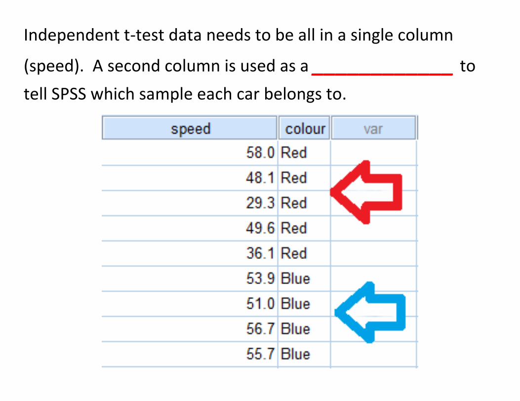
Independent t-test data needs to be all in a single column

(speed). A second column is used as a ____________ to

tell SPSS which sample each car belongs to.

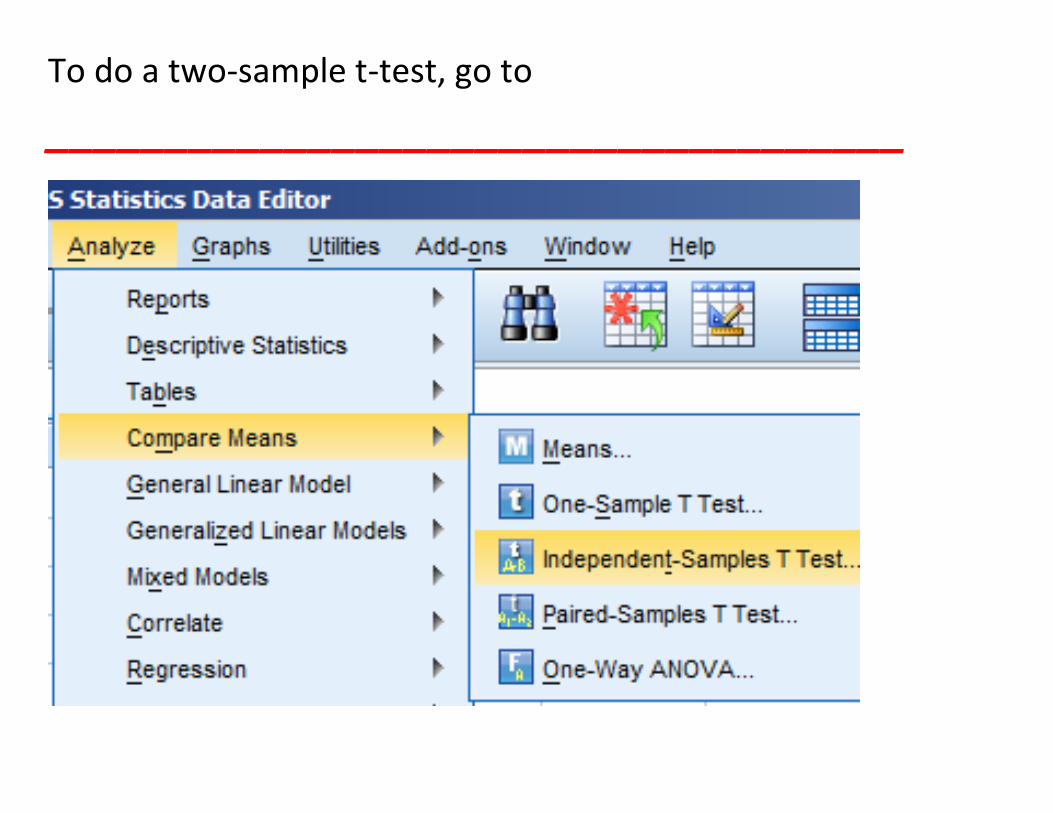
To do a two-sample t-test, go to

____________________________________

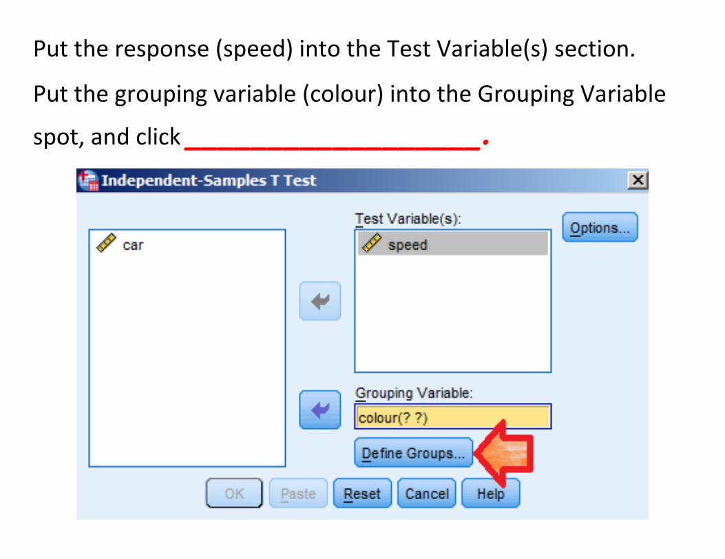
Put the response (speed) into the Test Variable(s) section.

Put the grouping variable (colour) into the Grouping Variable

spot, and click __________________.

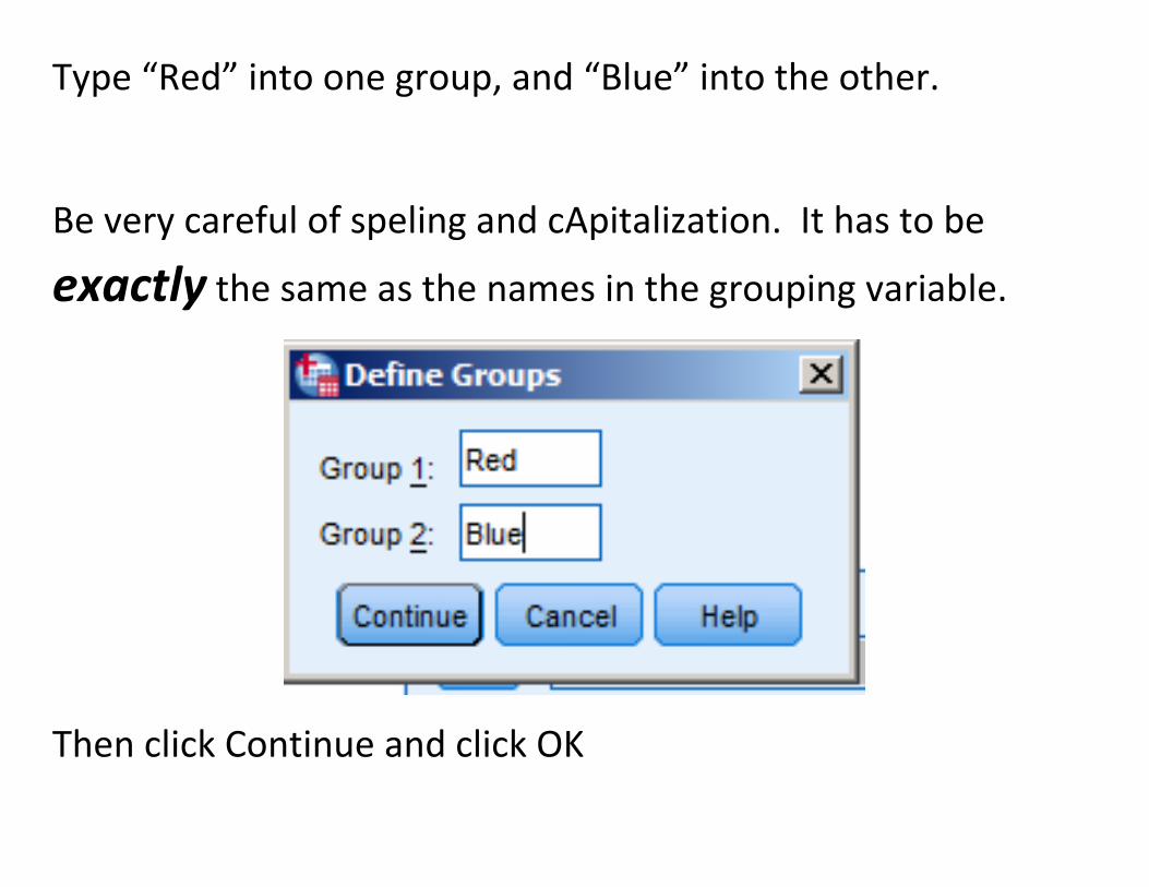
Type “Red” into one group, and “Blue” into the other.

Be very careful of speling and cApitalization. It has to be

exactly the same as the names in the grouping variable.

Then click Continue and click OK

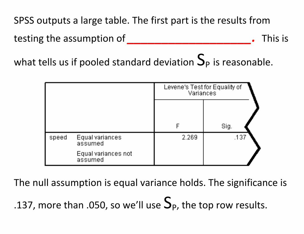
SPSS outputs a large table. The first part is the results from

testing the assumption of __________________. This is

what tells us if pooled standard deviation SP is reasonable.

The null assumption is equal variance holds. The significance is

.137, more than .050, so we’ll use SP, the top row results.

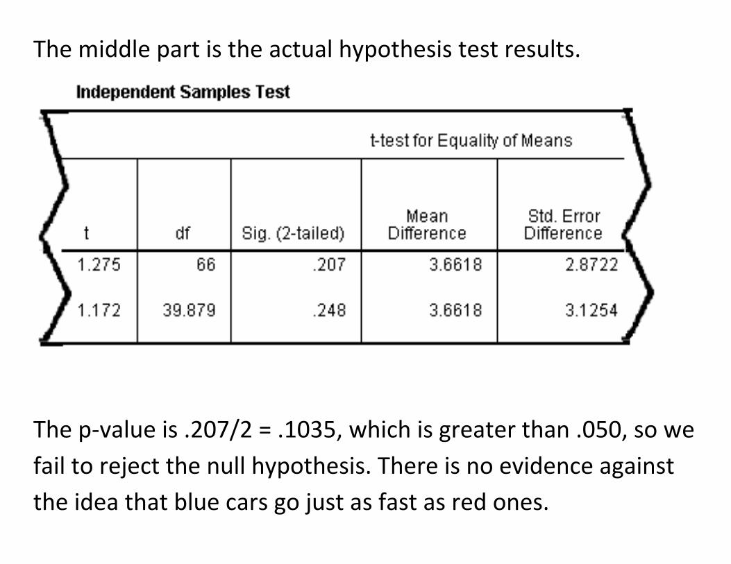
The middle part is the actual hypothesis test results.

The p-value is .207/2 = .1035, which is greater than .050, so we

fail to reject the null hypothesis. There is no evidence against

the idea that blue cars go just as fast as red ones.

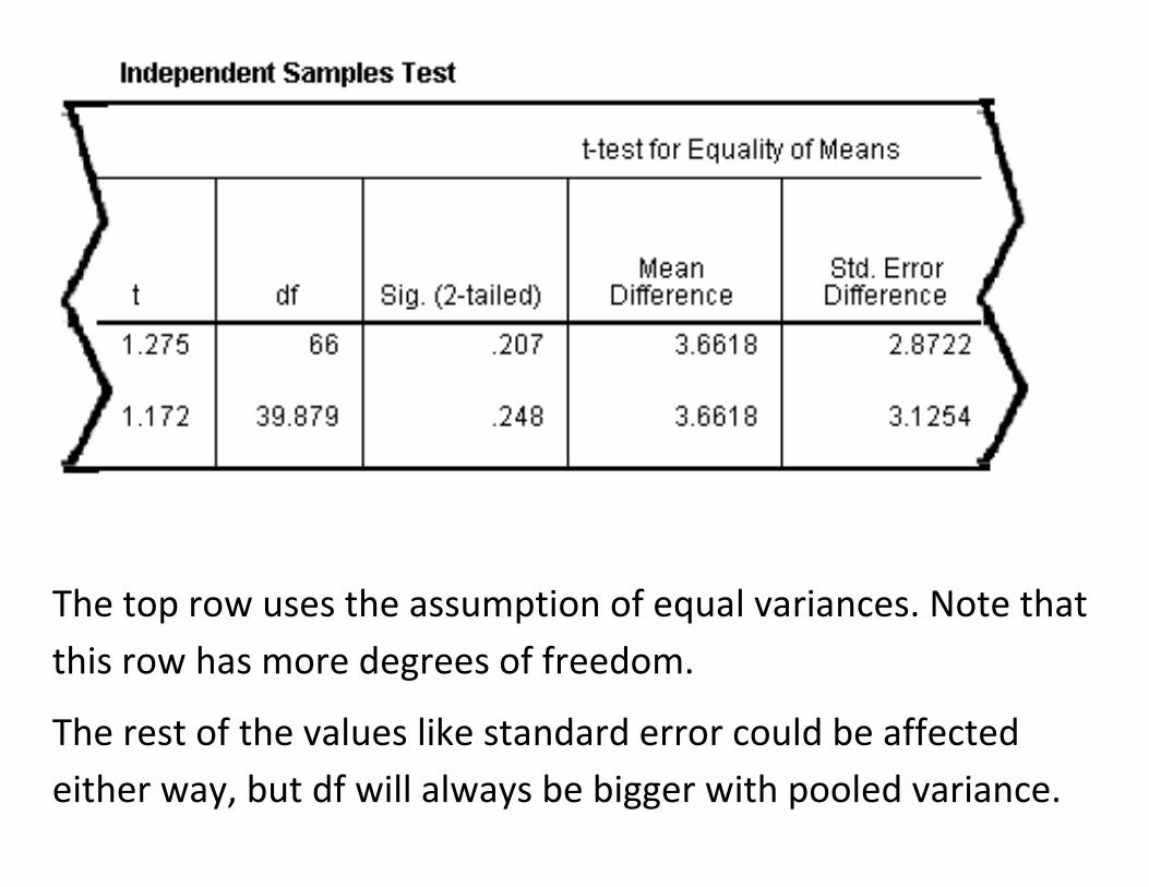
The top row uses the assumption of equal variances. Note that

this row has more degrees of freedom.

The rest of the values like standard error could be affected

either way, but df will always be bigger with pooled variance.

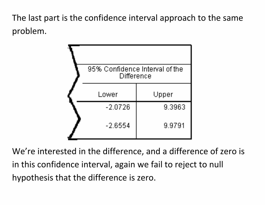
The last part is the confidence interval approach to the same

problem.

We’re interested in the difference, and a difference of zero is

in this confidence interval, again we fail to reject to null

hypothesis that the difference is zero.

Computers: Wizardous or Lizardous?

SPSS and two samples, Part 2: Red cars are for girls.

If we have data in a 0-1 format, we can do two-sample t-tests

on proportions as well.

The last variable in the Red Cars dataset is Gender, meaning

the gender of the driver, it’s coded 0 for male and 1 for female.

We want to know if there if the proportion of red car drivers

that are female is different than the proportion of blue car

drivers that are female.

(Two-tailed, two-sample t-test)

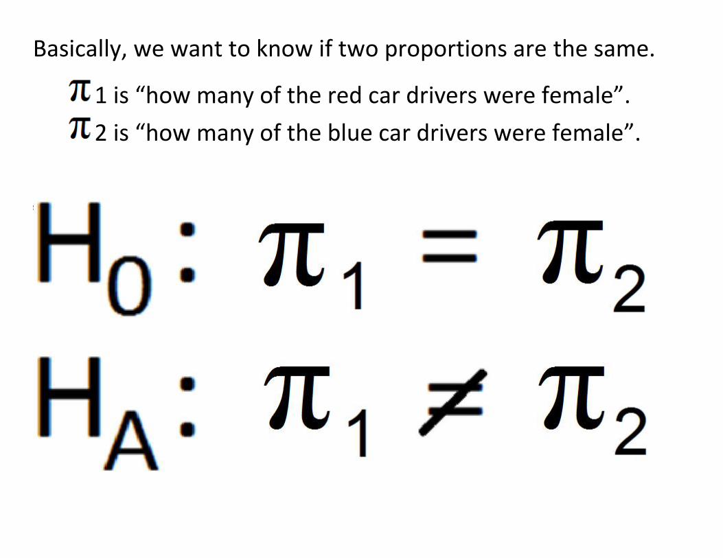
Basically, we want to know if two proportions are the same.

1 is “how many of the red car drivers were female”.

2 is “how many of the blue car drivers were female”.

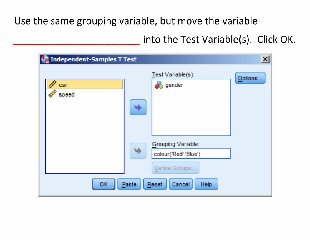
Use the same grouping variable, but move the variable

__________________ into the Test Variable(s). Click OK.

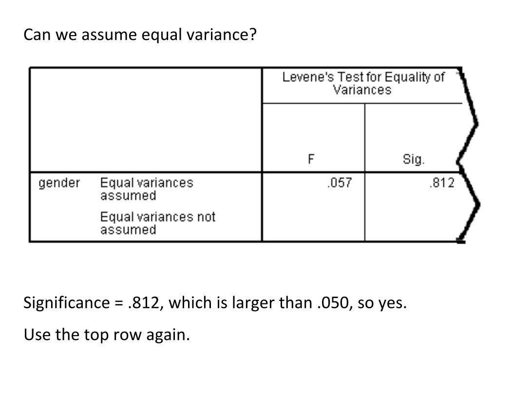
Can we assume equal variance?

Significance = .812, which is larger than .050, so yes.

Use the top row again.

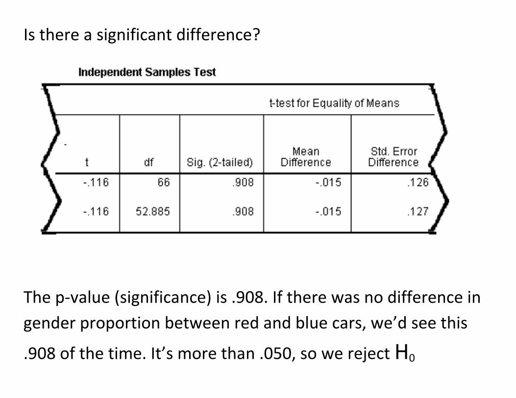
Is there a significant difference?

The p-value (significance) is .908. If there was no difference in

gender proportion between red and blue cars, we’d see this

.908 of the time. It’s more than .050, so we reject H0

Uff, stats… so much work.

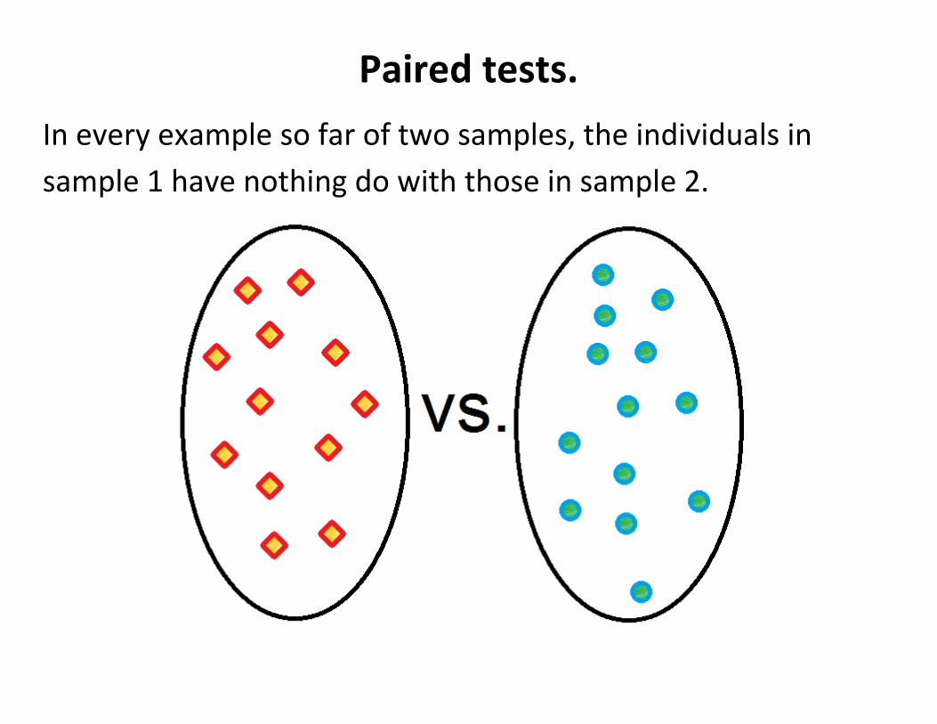
Paired tests.

In every example so far of two samples, the individuals in

sample 1 have nothing do with those in sample 2.

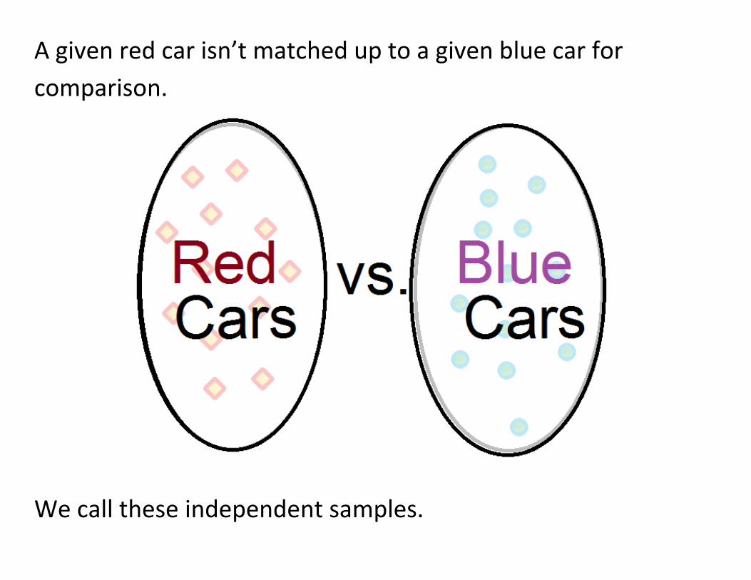
A given red car isn’t matched up to a given blue car for

comparison.

We call these independent samples.

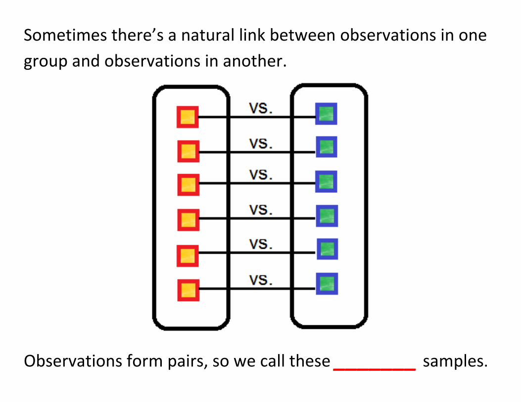
Sometimes there’s a natural link between observations in one

group and observations in another.

Observations form pairs, so we call these _______ samples.

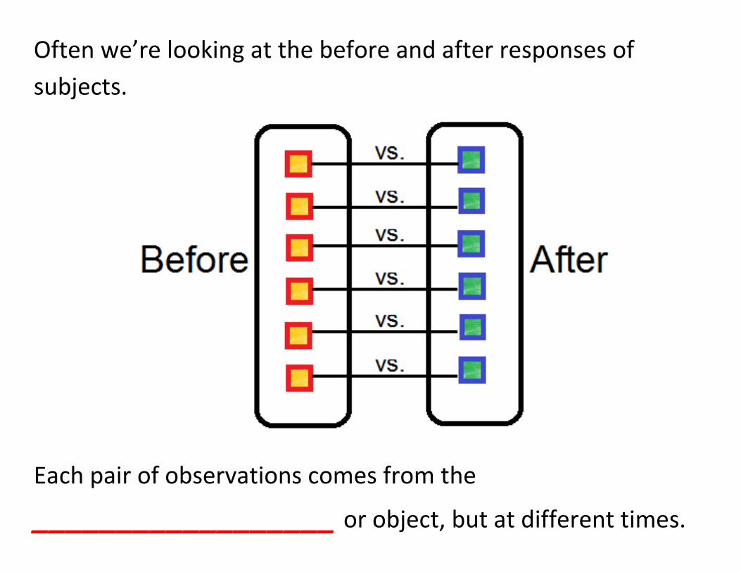
Often we’re looking at the before and after responses of

subjects.

Each pair of observations comes from the

__________________ or object, but at different times.

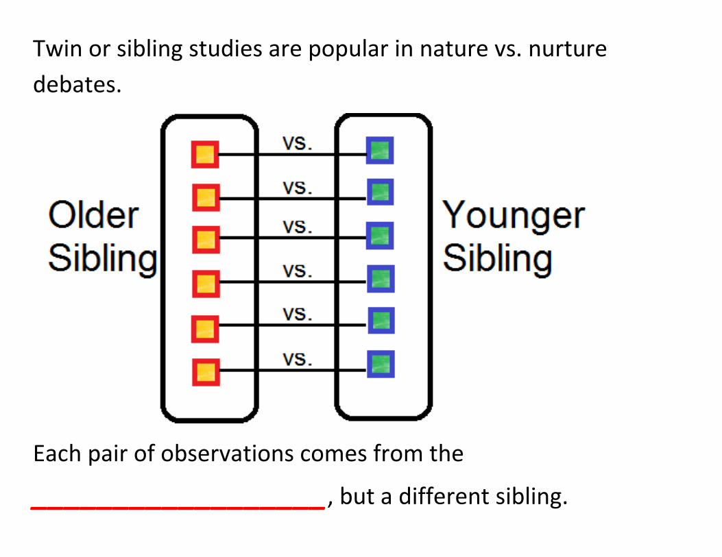
Twin or sibling studies are popular in nature vs. nurture

debates.

Each pair of observations comes from the

__________________, but a different sibling.

SPSS and two sample tests – Part 3.

Is there an historical difference in gas prices across Vancouver?

We have the monthly average gas prices for 62 months in

Burnaby, Coquitlam, and Delta.

We want to know, is there a difference betweeen Burnaby and

Coquitlam prices. (Two-tailed test)

Each pair of observations has a link: They come from the

__________________. A common link means a paired

t-test is appropriate.

Some of the variation is going to be due to factors beyond

Vancouver, like the season and global economics and politics,

that could affect gas prices.

Since many of the effects happen at the same time, we roll

them into a time variable (month). Using the time variable like

this is a common practice.

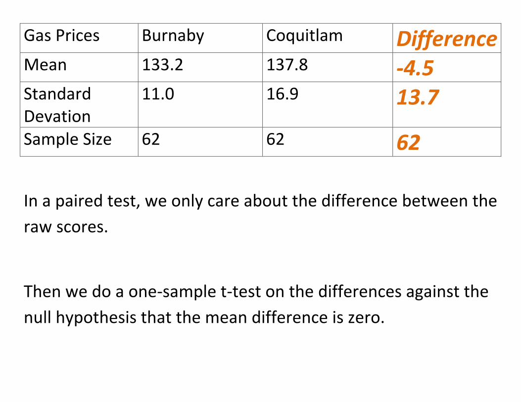
Gas Prices Burnaby Coquitlam Difference

Mean 133.2 137.8 -4.5 Standard Devation

11.0 16.9 13.7

Sample Size 62 62 62

In a paired test, we only care about the difference between the

raw scores.

Then we do a one-sample t-test on the differences against the

null hypothesis that the mean difference is zero.

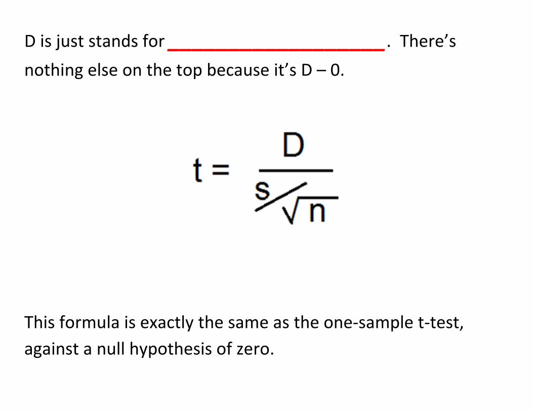
D is just stands for __________________. There’s

nothing else on the top because it’s D – 0.

This formula is exactly the same as the one-sample t-test,

against a null hypothesis of zero.

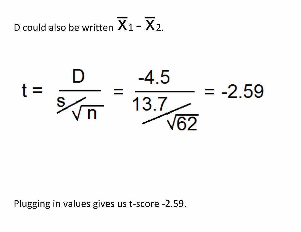
D could also be written 1 - 2.

Plugging in values gives us t-score -2.59.

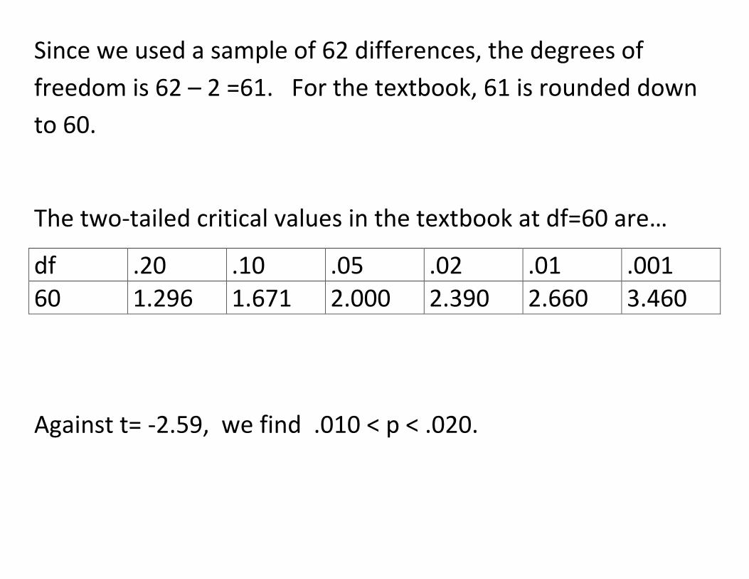
Since we used a sample of 62 differences, the degrees of

freedom is 62 – 2 =61. For the textbook, 61 is rounded down

to 60.

The two-tailed critical values in the textbook at df=60 are…

df .20 .10 .05 .02 .01 .001 60 1.296 1.671 2.000 2.390 2.660 3.460

Against t= -2.59, we find .010 < p < .020.

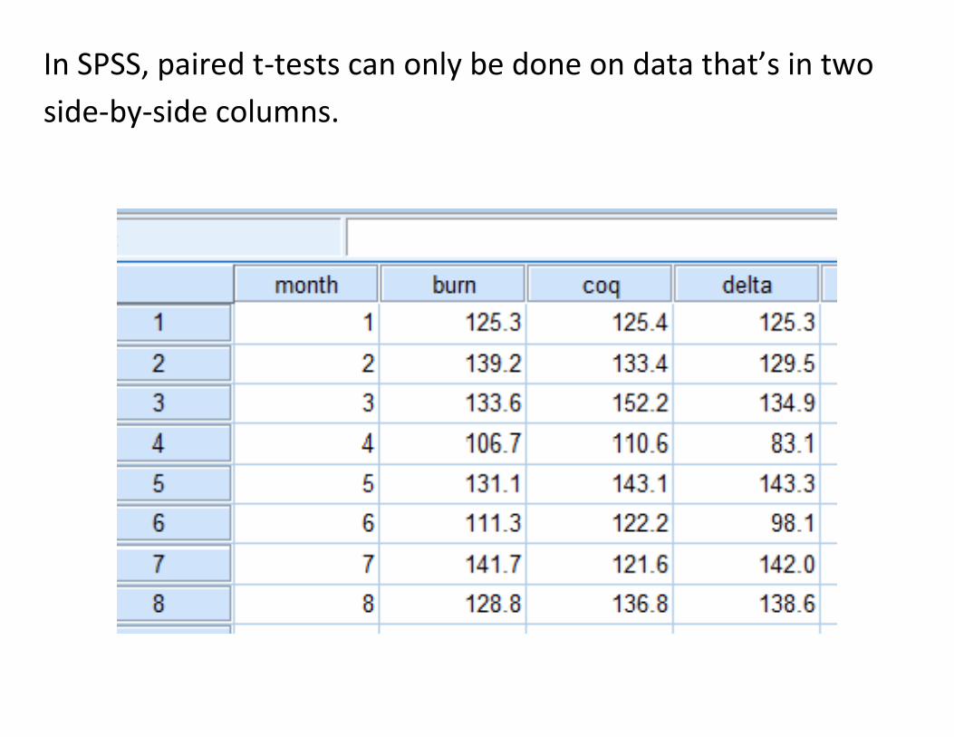
In SPSS, paired t-tests can only be done on data that’s in two

side-by-side columns.

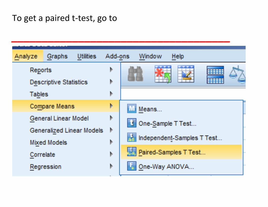
To get a paired t-test, go to

____________________________________

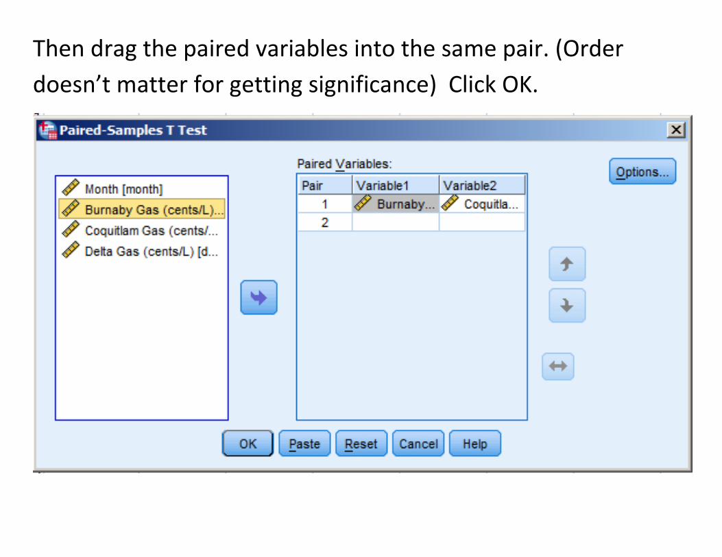
Then drag the paired variables into the same pair. (Order

doesn’t matter for getting significance) Click OK.

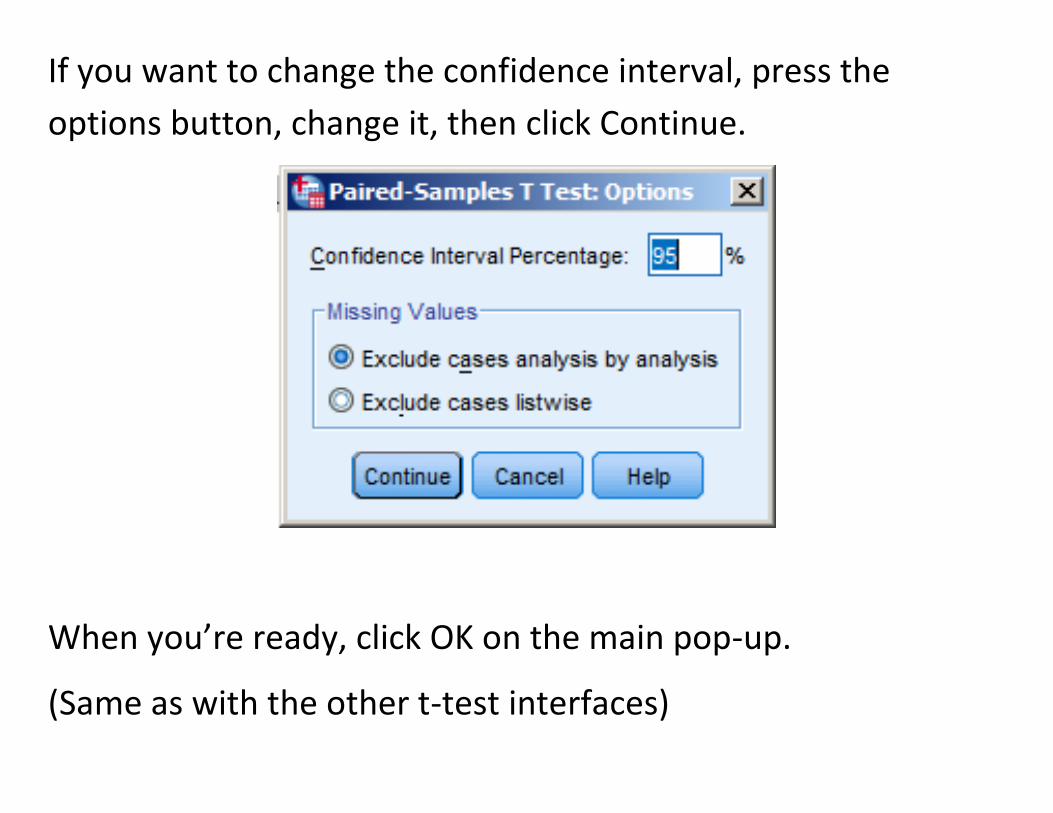
If you want to change the confidence interval, press the

options button, change it, then click Continue.

When you’re ready, click OK on the main pop-up.

(Same as with the other t-test interfaces)

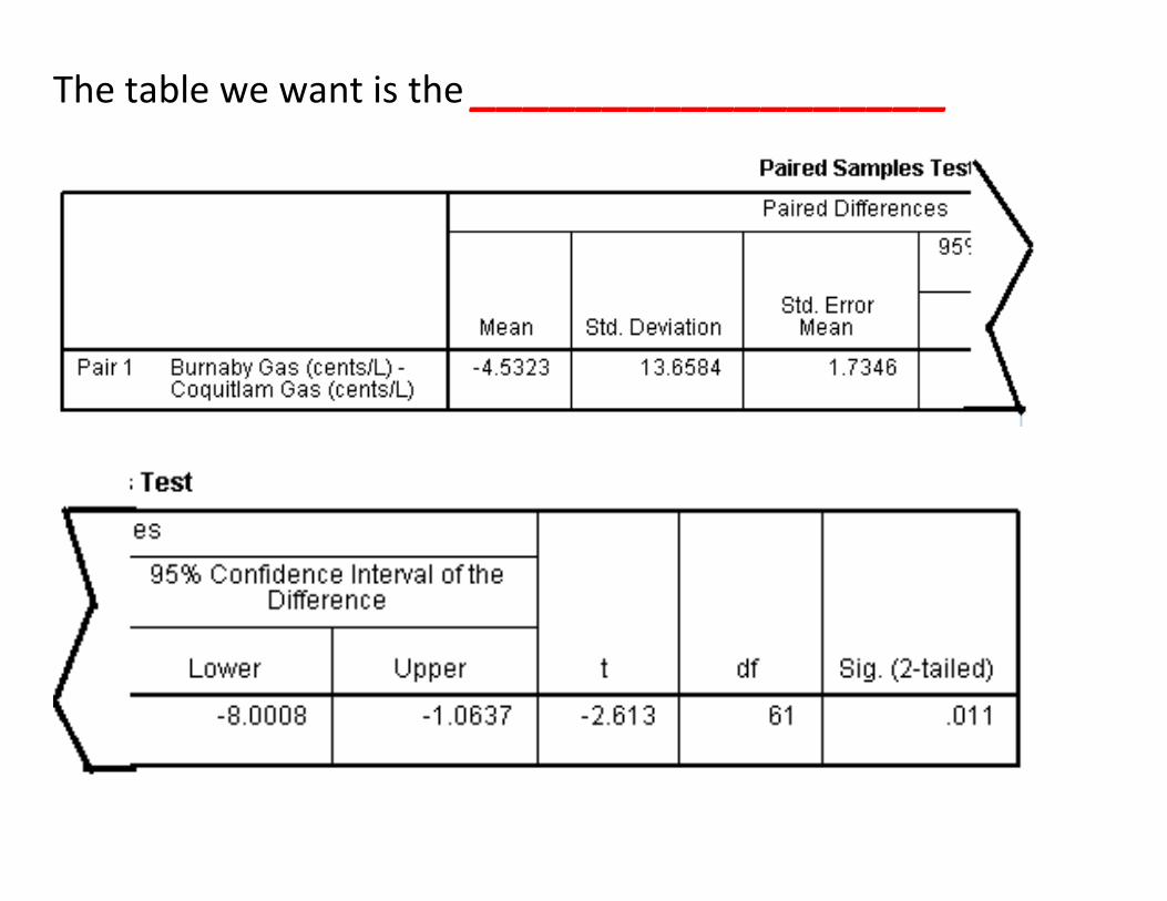
The table we want is the __________________

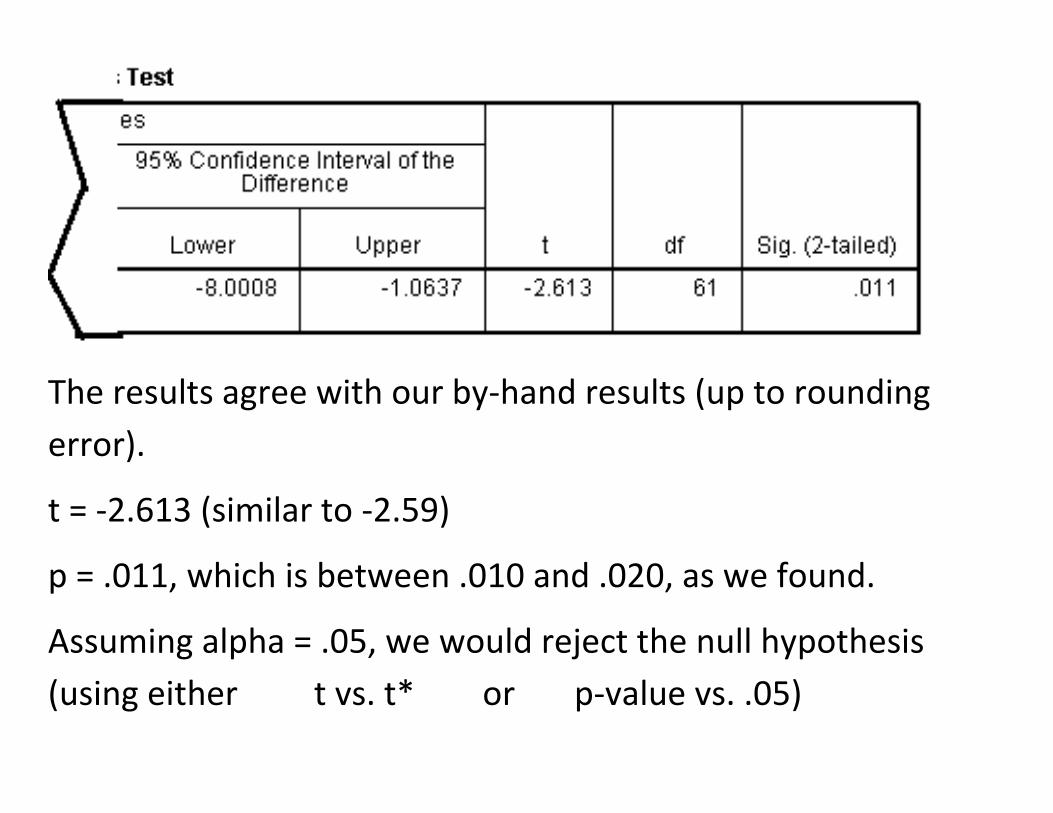
The results agree with our by-hand results (up to rounding

error).

t = -2.613 (similar to -2.59)

p = .011, which is between .010 and .020, as we found.

Assuming alpha = .05, we would reject the null hypothesis

(using either t vs. t* or p-value vs. .05)

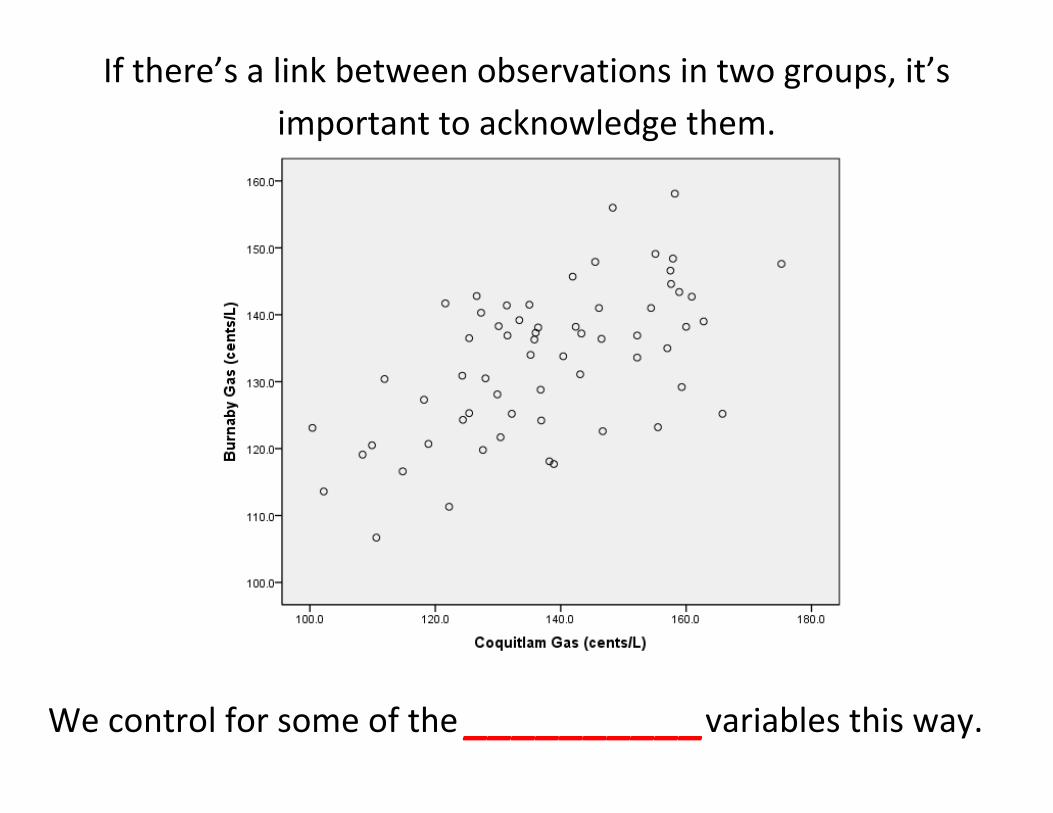
If there’s a link between observations in two groups, it’s

important to acknowledge them.

We control for some of the __________variables this way.

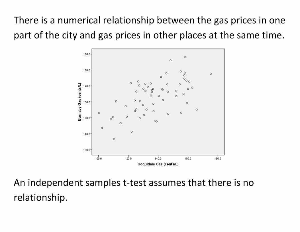
There is a numerical relationship between the gas prices in one

part of the city and gas prices in other places at the same time.

An independent samples t-test assumes that there is no

relationship.

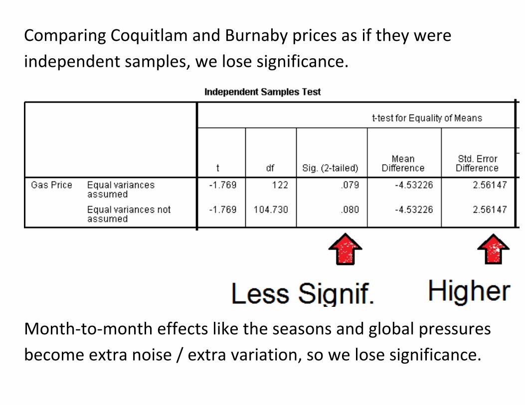
Comparing Coquitlam and Burnaby prices as if they were

independent samples, we lose significance.

Month-to-month effects like the seasons and global pressures

become extra noise / extra variation, so we lose significance.

Next class: Type I and Type II Errors

Chapter 7 Wrap-Up, extra examples.