Embed Size (px)
Citation preview

Hypergeometric forms for Ising-class integrals
D.H. Bailey∗, D. Borwein†, J.M. Borwein‡
R.E. Crandall§
September 11, 2006
Abstract: We apply experimental-mathematical principles to analyze integrals
Cn,k :=1n!
∫ ∞
0
· · ·∫ ∞
0
dx1 dx2 · · · dxn
(coshx1 + · · ·+ coshxn)k+1.
These are generalizations of a previous integral Cn := Cn,1 relevant to theIsing theory of solid-state physics [8]. We find representations of the Cn,k interms of Meijer G-functions and nested-Barnes integrals. Our investigationsbegan by computing 500-digit numerical values of Cn,k for all integers n, kwhere n ∈ [2, 12] and k ∈ [0, 25]. We found that some Cn,k enjoy exact eval-uations involving Dirichlet L-functions or the Riemann zeta function. In theprocess of analyzing hypergeometric representations, we found—experimentallyand strikingly—that the Cn,k almost certainly satisfy certain inter-indicial re-lations including discrete k-recursions. Using generating functions, differentialtheory, complex analysis, and Wilf–Zeilberger algorithms we are able to provesome central cases of these relations.
∗Lawrence Berkeley National Laboratory, Berkeley, CA 94720, [email protected]. Sup-ported in part by the Director, Office of Computational and Technology Research, Division ofMathematical, Information, and Computational Sciences of the U.S. Department of Energy,under contract number DE-AC02-05CH11231.
†Department of Mathematics University of Western Ontario, London, ONT, N6A 5B7 ,Canada, [email protected]. Supported in part by NSERC.
‡Faculty of Computer Science, Dalhousie University, Halifax, NS, B3H 2W5, Canada,[email protected]. Supported in part by NSERC and the Canada Research Chair Pro-gramme.
§Center for Advanced Computation, Reed College, Portland OR, [email protected].
1

1 Background and nomenclature
The primary entities on which the present work will focus are the n-dimensionalintegrals
Cn,k :=1n!
∫ ∞
−∞· · ·
∫ ∞
−∞
dx1 dx2 · · · dxn
(coshx1 + · · ·+ coshxn)k+1. (1)
These integrals are well defined—in fact absolutely convergent—for any positiveinteger n and any complex k ∈ K where we speak of the open half-plane
K := (z ∈ C : <(z) > −1) .
The integrals Cn,k can be traced back to the Ising theory of solid-statephysics. As summarized in a previous work [8], there is interest in giving closedforms and growth bounds for n-dimensional Ising susceptibility integrals
Dn :=4n!
∫ ∞
0
· · ·∫ ∞
0
∏i<j
(ui−uj
ui+uj
)2
(∑nj=1(uj + 1/uj)
)2
du1
u1· · · dun
un. (2)
These Dn appear—with various normalizations—in the standard Ising litera-ture [29, 30, 40, 41, 42, 43]. The quest for closed forms for Ising susceptibilityintegrals thus led to a definition in [8] of a class of structurally similar integrals,among which is the structure (2) but without the permutation product in theintegrand, namely
Cn :=4n!
∫ ∞
0
· · ·∫ ∞
0
1(∑nj=1(uj + 1/uj)
)2
du1
u1· · · dun
un, (3)
which, as can be seen via a transformation uk → exk is the case Cn,1 of the keydefinition (1).
A brief digression here is worthwhile. There is an even more general class ofintegrals that likewise admit of analytical promise. We may define, for integern, complex k, and an n-vector ~r := (r1, . . . , rn) of complex numbers the entities
Cn,k,~r :=1n!
∫ ∞
−∞· · ·
∫ ∞
−∞
∏nj=1 cosh(rjxj)
(coshx1 + · · ·+ coshxn)k+1dx1 · · · dxn. (4)
Absolute convergence of the integral is assured on the condition that k lie inthe translated half-plane K + < (
∑rj). Thus we can restrict indices to obtain
integrals of our primary interest, e.g.
Cn,k := Cn,k,~0, (5)Cn := Cn,1 := Cn,1,~0. (6)
One reason to contemplate these generalized Cn,k,~r is that they enjoy certaincombinatorial relations when cast in so-called Bessel-kernel form, as we shall
2
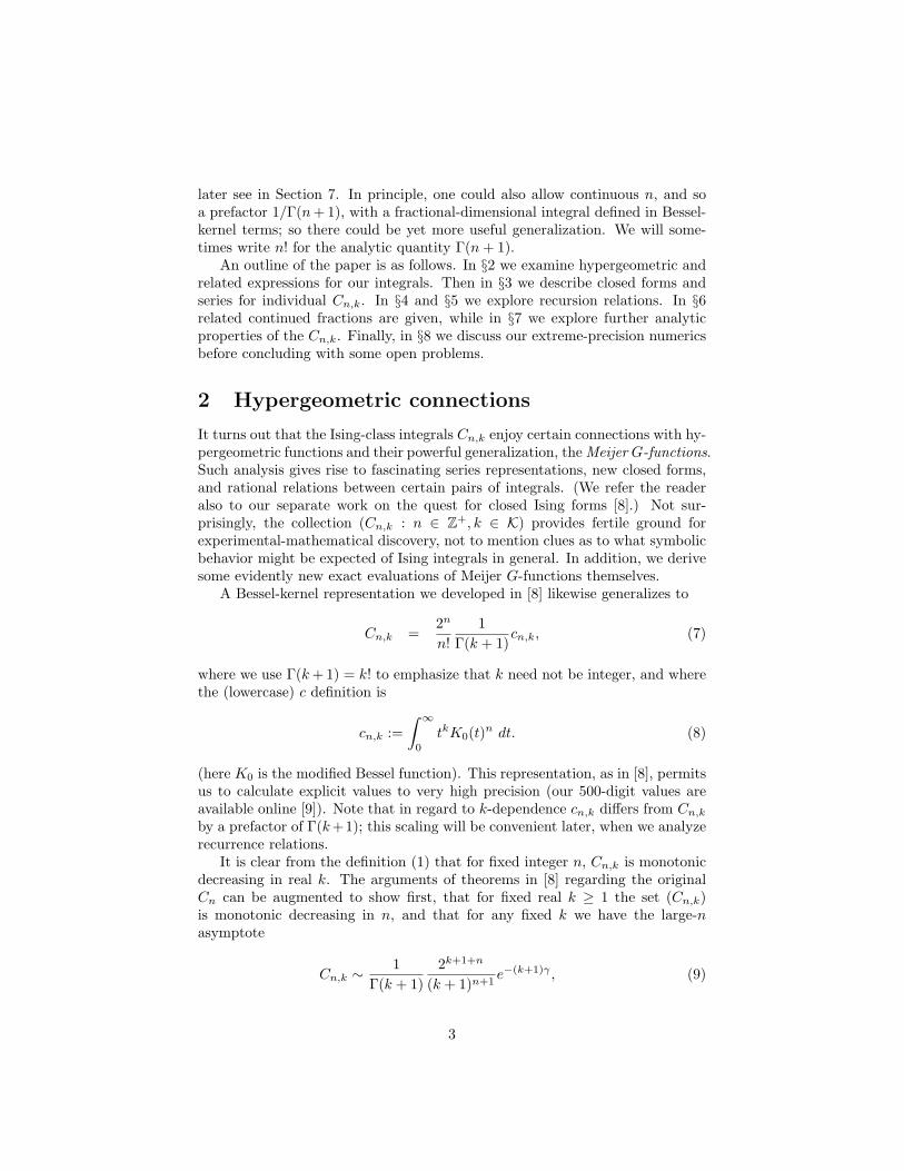
later see in Section 7. In principle, one could also allow continuous n, and soa prefactor 1/Γ(n + 1), with a fractional-dimensional integral defined in Bessel-kernel terms; so there could be yet more useful generalization. We will some-times write n! for the analytic quantity Γ(n + 1).
An outline of the paper is as follows. In §2 we examine hypergeometric andrelated expressions for our integrals. Then in §3 we describe closed forms andseries for individual Cn,k. In §4 and §5 we explore recursion relations. In §6related continued fractions are given, while in §7 we explore further analyticproperties of the Cn,k. Finally, in §8 we discuss our extreme-precision numericsbefore concluding with some open problems.
2 Hypergeometric connections
It turns out that the Ising-class integrals Cn,k enjoy certain connections with hy-pergeometric functions and their powerful generalization, the Meijer G-functions.Such analysis gives rise to fascinating series representations, new closed forms,and rational relations between certain pairs of integrals. (We refer the readeralso to our separate work on the quest for closed Ising forms [8].) Not sur-prisingly, the collection (Cn,k : n ∈ Z+, k ∈ K) provides fertile ground forexperimental-mathematical discovery, not to mention clues as to what symbolicbehavior might be expected of Ising integrals in general. In addition, we derivesome evidently new exact evaluations of Meijer G-functions themselves.
A Bessel-kernel representation we developed in [8] likewise generalizes to
Cn,k =2n
n!1
Γ(k + 1)cn,k, (7)
where we use Γ(k + 1) = k! to emphasize that k need not be integer, and wherethe (lowercase) c definition is
cn,k :=∫ ∞
0
tkK0(t)n dt. (8)
(here K0 is the modified Bessel function). This representation, as in [8], permitsus to calculate explicit values to very high precision (our 500-digit values areavailable online [9]). Note that in regard to k-dependence cn,k differs from Cn,k
by a prefactor of Γ(k+1); this scaling will be convenient later, when we analyzerecurrence relations.
It is clear from the definition (1) that for fixed integer n, Cn,k is monotonicdecreasing in real k. The arguments of theorems in [8] regarding the originalCn can be augmented to show first, that for fixed real k ≥ 1 the set (Cn,k)is monotonic decreasing in n, and that for any fixed k we have the large-nasymptote
Cn,k ∼1
Γ(k + 1)2k+1+n
(k + 1)n+1e−(k+1)γ , (9)
3

for which our original, canonical case in [8] reads Cn = Cn,1 ∼n 2e−2γ ≈0.63047 . . .. This asymptotic behavior is revealed by extreme-precision numeri-cal values for Cn. An example of the data downloadable at [9] is the following,where the asymptote 2e−2γ is evident:
n Cn
4 0.70119986017642999981651392754834582794624200386529. . .16 0.63050394617323726350529565756068741948431621720810. . .64 0.63047350337438679648836208816533862535998880860015. . .
256 0.63047350337438679612204019271087890435458707871273. . .1024 0.63047350337438679612204019271087890435458707871273. . .
Another observation on the generalization Cn,k,~r is in order. Some idea ofthe power of Bessel representation such as (7) can be gleaned by the observationthat, for vector ~r := (p, p, . . . , p) = (p) we have again a 1-dimensional integral
Cn,k,(p) :=2n
n!1
Γ(k + 1)
∫ ∞
0
tkKp(t)n dt.
It is interesting that for p a half-odd integer, the Bessel function is elementaryand we routinely obtain closed forms. For example, for general complex k weinfer
C4,k,(3/2,3/2,3/2,3/2) =21−2kπ2Γ(k − 5)
3Γ(k + 1)(k4 + 2k3 − 25k2 − 10k + 56
)of which an instance is
C4,6,(3/2)
= 103π2/552960.
Though such cases do not shed much light on our main theme—the Cn,k themselves—these tractable cases do suggest such notions as analytic continuation (in k,beyond the relevant half-plane) as well as the appearance of polynomials in k.
We shall be analyzing series representations and closed forms for variousCn,k. To this end, we state some exact integrals based on the Adamchik algo-rithm described in [2]:
c1,k =∫ ∞
0
tkK0(t) dt = 2k−1Γ(
k + 12
)2
, (10)
c2,k =∫ ∞
0
tkK20 (t) dt =
√π Γ
(k+12
)3
4 Γ(
k2 + 1
) , (11)
c3,k =∫ ∞
0
tkK30 (t) dt = 2k−2
√π G3,2
3,3
(4
∣∣∣∣ 1−k2 , 1−k
2 , 12
0, 0, 0
), (12)
4
where the relevant Meijer G-function here is
G :=1
2πi
∫C
Γ2((k + 1)/2− s)Γ3(s)Γ(s + 1/2)
4−s ds.
Finally, we have
c4,k =∫ ∞
0
tkK40 (t) dt =
18πG3,3
4,4
(1
∣∣∣∣ 1, 1, 1, k+22
k+12 , k+1
2 , k+12 , 1
2
), (13)
where in this case the relevant Meijer G-function is
G :=1
2πi
∫C
Γ3(−s)Γ3((k + 1)/2 + s)Γ(1 + k/2 + s)Γ(1/2− s)
ds.
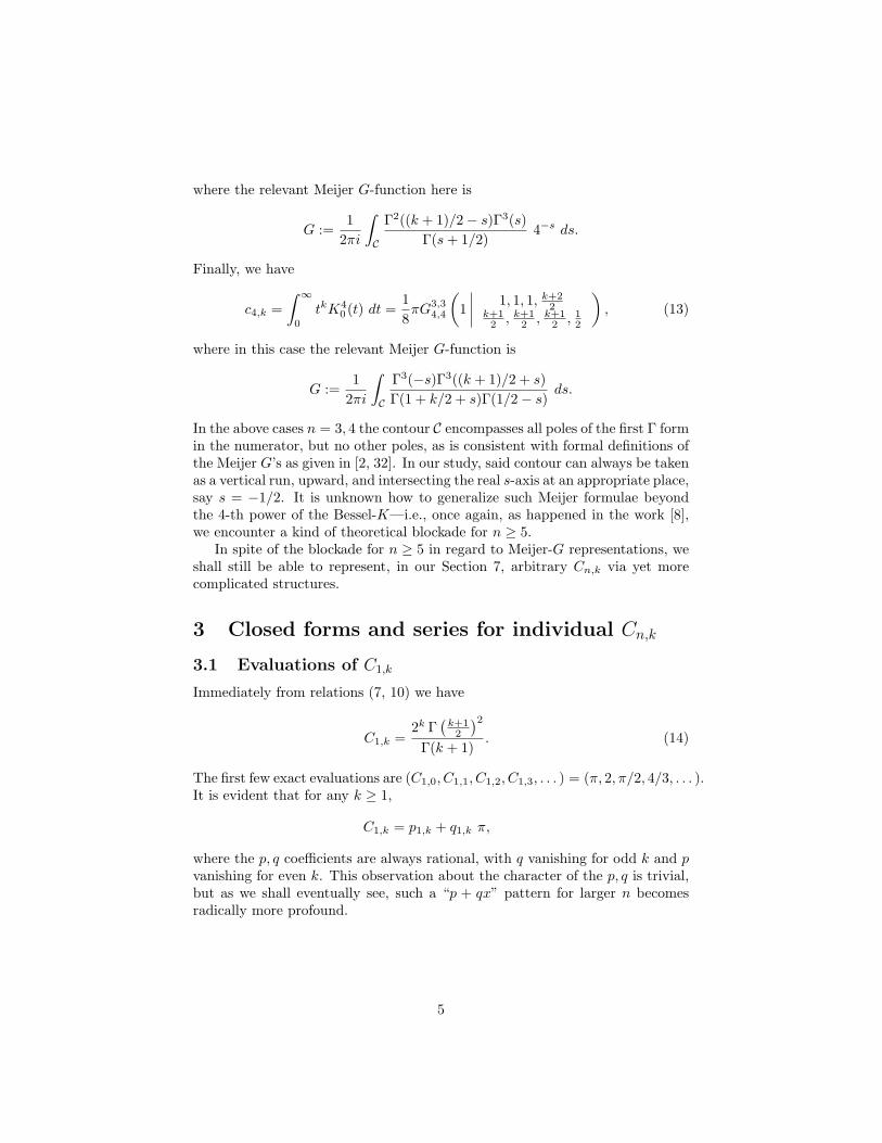
In the above cases n = 3, 4 the contour C encompasses all poles of the first Γ formin the numerator, but no other poles, as is consistent with formal definitions ofthe Meijer G’s as given in [2, 32]. In our study, said contour can always be takenas a vertical run, upward, and intersecting the real s-axis at an appropriate place,say s = −1/2. It is unknown how to generalize such Meijer formulae beyondthe 4-th power of the Bessel-K—i.e., once again, as happened in the work [8],we encounter a kind of theoretical blockade for n ≥ 5.
In spite of the blockade for n ≥ 5 in regard to Meijer-G representations, weshall still be able to represent, in our Section 7, arbitrary Cn,k via yet morecomplicated structures.
3 Closed forms and series for individual Cn,k
3.1 Evaluations of C1,k
Immediately from relations (7, 10) we have
C1,k =2k Γ
(k+12
)2
Γ(k + 1). (14)
The first few exact evaluations are (C1,0, C1,1, C1,2, C1,3, . . . ) = (π, 2, π/2, 4/3, . . . ).It is evident that for any k ≥ 1,
C1,k = p1,k + q1,k π,
where the p, q coefficients are always rational, with q vanishing for odd k and pvanishing for even k. This observation about the character of the p, q is trivial,but as we shall eventually see, such a “p + qx” pattern for larger n becomesradically more profound.
5

n k Cn,k
1 any2kΓ( k+1
2 )2
k! = p1,k + q1,k π
2 any√
πΓ( k+12 )3
2Γ( k2 +1)Γ(k+1)
= p2,k + q2,k π2
3 0 Elliptic form (21)
3 1 C3 = L−3(2) (see [8])
3 2 Elliptic form (24)
3 3 C3,3 = 29 L−3(2)− 4
27
3 any odd p3,k + q3,k L−3(2), Series (16)
3 any even Order-2 recursion (Thm. 5), Series (17)
3 any complex Meijer integral (12)
4 0 Series (31)
4 1 C4 = 712 ζ(3) (see [8])
4 3 C4,3 = 7288 ζ(3)− 1
48
4 any odd p4,k + q4,k ζ(3)
4 any even Order-2 recursion (Thm. 5)
4 any complex Meijer integral (13)
5 any complex Nested-Barnes integral (55), Series (58)
large fixed ∼ 1k!
2k+1+n
(k+1)n+1 e−(k+1)γ
Table 1: Proven closed forms, series, and relations for the Cn,k. Every
p or q coefficient above is proven rational, with the q having explicit finite forms.
Our searches have uncovered no other closed forms, or pairwise rational relations not
implicit above. Conjecture 1 gives a general recursion relation for complex k.6

3.2 Evaluations of C2,k
Next, from relations (7, 11) we obtain
C2,k =√
π Γ(
k+12
)3
2 Γ(
k2 + 1
)Γ(k + 1)
, (15)
with the first few being (C2,0, C2,1, C2,2, C2,3, . . . ) = (π2/2, 1, π2/32, 1/9, . . . ).In this n = 2 case we have
C2,k = p2,k + q2,k π2,
with the same vanishing rule on the rational p, q multipliers as for n = 1.
3.3 Evaluations of C3,k
After resolving all Cn,k for n = 1, 2 as above, the case n = 3 on Cn,k suddenlybecomes nontrivial, yet there are various approaches that yield new insight; atthe very least, new closed-form evaluations of the appropriate Meijer-G. Choos-ing a contour and performing residue calculus (we leave out the intricate details)on the Meijer-G for identity (12), one may obtain quite efficient series develop-ments. To summarize, define µ := b(k − 2)/2c and a polynomial
Pµ(x) :=µ∏
a=0
(x− a)2,
and an alternating harmonic number
H(−1)c := 1− 1
2+
13− · · · ± 1
c
with H(−1)0 := 0. Then, for odd k, the residue calculus yields a linearly conver-
gent series
C3,k =2k√
π
3!k!
∞∑h=µ+1
Pµ(h)4h
Γ(h + 1)Γ(h + 3/2)
(H
(−1)2h+1 −
12
P ′µ(h)Pµ(h)
). (16)
Similarly, for even k, one obtains
C3,k =2k+1
√π
3!k!
∞∑h=µ+1
Pµ(h)4h
Γ3(h + 1/2)Γ3(h + 1)
(4 log 2− 3H
(−1)2h − 1
2P ′µ(h)Pµ(h)
). (17)
3.3.1 The C3,even integrals
Yet another surprise in the world of Ising-class integrals is that the C3,even seemto be more mysterious than the C3,odd. One way to think of this dichotomy isto observe the way that gamma functions appear in the respective series (16,
7

17). One may employ special hypergeometric identities, which we found inMathematica and reconfirmed in Maple, such as
∞∑h=0
Γ(h + 1)Γ(h + 3/2)
sin2h θ =4√π
θ
sin(2θ), (18)
σ0(θ) :=∞∑
h=0
Γ3(h + 1/2)Γ3(h + 1)
sin2h θ =4√π
K2
(sin
θ
2
), (19)
where in the second identity K(k) is the (complete) elliptic integral of the firstkind with modulus k.1 We may also employ an integral identity
4 log 2− 3H(−1)2h =
∫ 1
0
1 + 3t2h
1 + tdt = log 2 + 3
∫ 1
0
t2h
1 + tdt.
Putting this all together for the special case
C3,0 =√
π
3
∞∑h=0
14h
Γ3(h + 1/2)Γ3(h + 1)
(4 log 2− 3H
(−1)2h
)(20)
we arrive at the peculiar elliptic representation
C3,0 =43K2
(sin
π
12
)log 2 + 8
∫ π/6
0
K2(sin θ
2
)cos θ
1 + 2 sin θdθ. (21)
Moreover
K2(sin
π
12
)=
227
√3 3√
2 π4
Γ6 (2/3)=
3√
2√
324
β2
(13,13
)is the integral at the third singular value, k3 [16]. Correspondingly, the Clausenproduct identity [15, p. 50] shows
8∫ π/6
0
K2(sin θ
2
)cos θ
1 + 2 sin θdθ = π2
∫ 1
03F2
(1/2, 1/2, 1/2
1, 1 ;x2
4
)dx
x + 1.
This elliptic-cum-hypergeometric form is a rather erudite result for the relativelyinnocent-looking integral
C3,0 :=16
∫R3
dx dy dz
coshx + cosh y + cosh z.
There are other attractive representations equivalent to the elliptic form (21)such as
C3,0 = π
∫ ∞
0
∫ ∞
0
1√
x2 + 1√
y2 + 1√
(x + y)2 + 1dx dy.
1Here we use the convention K(k) =R π/20 (1 − k2 sin2 s)−1/2 ds. See [15, pg 199-200].
One should beware: Some symbolic systems use m := k2 as the argument; for example inMathematica one has EllipticK[m] := K(
√m).
8

We next observe that C3,2 possesses a corresponding closed form which alsoinvolves the elliptic integral of the second kind E(k3), [18]. This may be similarlyderived from (17) as follows.
Since P0(x) = x2, the building blocks for C3,2 are
σ1(θ) :=∞∑
h=0
h Γ3 (h + 1/2)Γ3 (h + 1)
sin2h θ (22)
=4√
π cos θ
{(E K)
(sin
θ
2
)− (cos2
θ
2) K2
(sin
θ
2
)}and
√π σ2(θ) :=
√π
∞∑h=0
h2 Γ3 (h + 1/2)Γ3 (h + 1)
sin2h θ (23)
=(cos θ + 1)
(cos2 θ + cos θ − 1
)cos3 θ
K2
(sin
θ
2
)− 2
(cos θ + 1) (2 cos θ − 1)cos3 θ
(E K)(
sinθ
2
)+
2cos2 θ
E2
(sin
θ
2
).
Thus, we may use (17) to write
C3,2 =2 log 2
3√
π σ2
(π
6
)− 2
3√
π σ1
(π
6
)+ 4
∫ π/6
0
√π σ2 (θ)
cos θ
1 + 2 sin θdθ.
(24)
Also, for θ = π/6, we have EK =(π + (2 + 2
√3)K2
)√3, see [18]. Thus,
using (24) we will get two more-complicated terms like the ones in C3,0 but nowinvolving both E and K. Note that cos π/12 = (
√3 + 1)/
√8 and sin π/12 =
(√
3− 1)/√
8 are reciprocals. Thus,√
π σ1
(π
6
)= −2
3K2
(sin
π
12
)+
23
π,
and√
π σ2
(π
6
)=
19
K2(sin
π
12
)+
π2
18K−2
(sin
π
12
).
In consequence of Theorem 5 below, all C3,even are superpositions of C3,0 andC3,2 with polynomial (in k) weights; thus, the C3,even can only involve algebraiccombinations of the numbers above, such as log 2, π and the elliptic evalua-tions/integrals. PSLQ suggests no relations exist between the seven monomialsimplicit in (24).
3.3.2 The C3,odd integrals
A first observation on the cases Ck,odd is as follows. We recall the exact L-function evaluation given in [8].:
C3 := C3,1 = L−3(2) :=∑m≥0
(1
(3m + 1)2− 1
(3m + 2)2
).
9

This knowledge on C3,1 leads, via (16), to the remarkable L-function identity
L−3(2) =23
∞∑h=0
1h + 1
1(2h + 1
h
) (1− 1
2+
13− · · ·+ 1
2h + 1
).
Observe that, via relation (12), this resolves the relevant Meijer-G in terms ofan L-function, which Meijer-G identity we believe to be new.
Now, the C3,odd seem to be pairwise rationally related, in the following sense.We discovered via numerical experiments the conjectures2
C3,3?= − 4
27+
29L−3(2),
C3,5?= − 92
1215+
881
L−3(2),
and several more, suggesting rational relations aC3,k+bC3,k′ = c for any distinctodd pair (k, k′), with a, b, c rational, a 6= b. These (n = 3, odd k) conjectureswere subsequently proven, as below. We should mention that we found no suchrational relations whatever between pairs of C3,even (see Conjecture 3).
One might conceivably use the residue expansion (16) to prove our experi-mentally detected relations. However there is another route, one that leads toan efficient algorithm for resolving the closed form of any C3,odd. We harkenback to the dimensional-reduction methods in [8] and reduce to a 2-dimensionalintegral
C3,k =√
π
3!Γ
(k+12
)Γ
(k2 + 1
) ∫ ∞
0
∫ ∞
0
dx dy
x y
1
{(1 + x + y)(1 + 1/x + 1/y)}(k+1)/2.
Now for odd k we may assign m := (k − 1)/2 and write∫ ∞
0
∫ ∞
0
dx dy
xy
1
{(1 + x + y)(1 + 1/x + 1/y)}(k+1)/2=
1m!2
(∂
∂α
∂
∂β
)m ∫ ∞
0
∫ ∞
0
dx dy
x y
1(α + x + y)(β + 1/x + 1/y)
∣∣α,β=1
The integral over x, say, may then be done, after which we put y = z/β toreveal that, remarkably, the α, β-dependent integral is really a function only ofthe product c := αβ. In fact,∫ ∞
0
∫ ∞
0
dx dy
x y
1(α + x + y)(β + 1/x + 1/y)
=∫ ∞
0
log(1 + 1/z) + log(c + z)z2 + cz + c
dz
=∫ 1
0
log c− 2 log t
t2 − ct + cdt,
2The notation?= means we experimentally suspect a given equality in absence of rigorous
proof. Of course, we shall prove these C3,odd closed forms, but we prefer to use?= when
reporting on initial numerical discovery.
10

the final integral being obtained by making the substitutions 1 + 1/z = 1/t andc + z = c/t respectively in the two parts of the preceding integral. Thus C3,k
reduces to
C3,k =2k+1
3! k!
(∂
∂α
∂
∂β
)m
Υ(αβ)∣∣α,β=1
, (25)
where
Υ(c) :=∫ 1
0
log√
c− log t
t2 − ct + cdt
=1
r+ − r−
(−1
2log(r+r−) log
1− 1/r−1− 1/r+
+ Li2(1/r−)− Li2(1/r+))
,
with
r± :=c±
√c2 − 4c
2.
Sure enough, for k = 1, and so m = 0 and no differentiation in (25), we obtainour original case C3 := C3,1 = (2/3)Υ(1) = L−3(2).
More generally, our finite representation (25) leads to a proof of the eval-uations above for C3,3 and C3,5 and indeed to a proof of our rational-relationconjecture. To this end, note that we can use the operator identity
∂2
∂α∂β=
∂
∂cc
∂
∂c.
valid on functions f where c = αβ. In expanded form this means(∂
∂α
∂
∂β
)m
f(c) =m∑
k=0
(m
k
)m!k!
ckf (m+k)(c).
From the above relations one may now derive, for nonnegative integers m,
C3,2m+1 =22m+1
3(2m + 1)(2mm
) m∑k=0
(m
k
)(m + k
k
)(−1)m+k+1I(m + k), (26)
where
I(ν) :=∫ 1
0
tν log t
(t2 − t + 1)ν+1dt. (27)
These observations lead us to
Theorem 1 For odd k ≥ 1, we have
C3,k = p3,k + q3,kL−3(2),
with the p, q coefficients always being rational, q3,k being given explicitly by (30)below.
11

Proof. In terms of the I function in (27), establishing the recursion
νI(ν − 1) + (2ν + 1)I(ν)− 3(ν + 1)I(ν + 1) +1ν
= 0 (28)
is enough to prove the theorem, because
I(0) = −32L−3(2), I(1) = −1
2L−3(2). (29)
One may also deriveI(ν) = aν + bνL−3(2)
with rational aν , bν satisfying the recursions
νaν−1 + (2ν + 1)aν − 3(ν + 1)aν+1 +1ν
= 0, a0 = a1 = 0;
νbν−1 + (2ν + 1)bν − 3(ν + 1)bν+1 +1ν
= 0, b0 = −32, b1 = −1
2.
So we now prove the recursion (28). For x ∈ (−1, 1) we have
y(x) :=∞∑
ν=0
I(ν)xν =∫ 1
0
log t
t2 − t(1 + x) + 1dt.
The recursion (28) thus holds if and only if
(x + 1)∞∑
ν=0
I(ν)xν +(
x + 2− 3x
) ∞∑ν=0
νI(ν)xν = I(0)− 3I(1) + log(1− x)
which is equivalent to y satisfying the differential equation
(x + 1)y + (x2 + 2x− 3)y′ = log(1− x)− 3L−3(2),
subject to the initial condition
y(0) = −32L−3(2).
Maple verifies that y(x) is indeed a solution. QED
It turns out to be possible to give a finite expression for the q3,k rational inTheorem 1. What may be called the terminal term of the chain differentiationin (25), namely{
Li2
(1r−
)− Li2
(1r +
)}·(
∂
∂α
∂
∂β
)m 1r+ − r−
∣∣α,β=1
,
gives the rational coefficient of L−3(2) as
q3,k =√
32k−1
k!
(∂
∂α
∂
∂β
)m 1(αβ(4− αβ))1/2
∣∣α,β=1
.
12

In particular, a finite expression for the general q coefficient is, with m :=(k − 1)/2,
q3,k =2k−1
k!
m∑j=0
(m
j
)(−1)m+j m!
j!
m+j∑i=0
(m + j
i
) (12
)i
(12
)m+j−i
(−1
3
)i
(30)
=√
322m−1 m!(2m− 1)!
m∑j=0
(−1)m+j (mj
)j! 2F1
(12 , 1
212 −m− j
;14
) j∏i=0
(12
+ m + i
).
The above analysis provides closed forms for the relevant Meijer G-functions.The method also provides an algorithm for exact evaluation of any C3,odd ratherefficiently.3 One may arrive quickly at such instances as
C3,15 :=13!
∫ ∞
−∞
∫ ∞
−∞
∫ ∞
−∞
dx dy dz
(coshx + cosh y + cosh z)16
= − 11884272896837856594575
+4139008
227988189L−3(2).
3.4 Evaluations of C4,k
We begin with the first case of (13). Residue calculus—again we omit theintricacies—gives series such as
C4,0 =124
∑h=0
(Γ4(h + 1/2)Γ4(h + 1)
)′′(31)
=13
∞∑h=0
Γ4(h + 1/2)Γ4(h + 1)
(8
(− log 2 + H
(−1)2h
)2
+ ζ(2)− 2H(−2)2h
),
where the double-derivative ′′ is with respect to h, and the new sum is
H(−2)µ := 1− 1/22 + 1/32 − · · · ± 1/µ2
with H(−2)0 := 0. However, just is with the C3,even cases of the previous section,
we know not a single closed form for C4,even and again, we found experimentallythat C4,odd are pairwise rationally related, meaning (see Table 1 for C4 := C4,1)that every C4,odd would be p + qζ(3) for rational p, q.
3One may explicitly differentiate and simplify in (25), but a faster algorithm is to use thefinite expression for q3,k given after Theorem 1, an extreme-precision evaluation of series (16),then a function such as Mathematica’s Rationalize[ ] to resolve p3,k. This amounts to aninteresting, systematic use of extreme precision within a general algorithm.
13

The finite-form evaluation of any C4,odd is achieved as follows. Define inte-grals
Uh :=iπ
2
∫ ∞
−∞
sinhπt
cosh3 πt
(−1
2+ it
)h
dt = (−1)h+1h(h− 1)ζ(2− h)
2π.
This later identity actually holds, for any integer h, with U1 := 1/(2π). Notethat under the further constraint h ≥ 0, the quantity πUh for h ≥ 0 is rational,as follows from the fact of known evaluations of ζ(2− h).
The relevance of the Uh is that a Meijer contour-integral as in (13) can bedeveloped like so:
G :=1
2πi
∫C
Γ3(−s)Γ3((k + 1)/2 + s)Γ(1 + k/2 + s)Γ(1/2− s)
ds
=iπ
2
∫ ∞
−∞
sinhπt
cosh3 πtF
(−1
2+ it
)dt,
where
F (s) :=Γ3((1 + k)/2 + s)Γ(1/2 + s)
Γ3(1 + s)Γ(1 + k/2 + s).
Now the key is, if we write
F (s) = f(s) + φ(s),
where we express F (s) =∑
j fjsj as a polynomial and an error term φ(s) = o(s),
then we can resolve the original Meijer-G by employing the Uh identity on themonomials fjs
j , and using residue calculus for the φ term, to write
G =∑
j
fjUj +12π
∞∑h=0
φ′′(h). (32)
This analysis now leads to a proof of the experimentally discovered conjectureon rational relations for any pair of C4,odd:
Theorem 2 For odd k ≥ 1, we have
C4,k = p4,k + q4,k ζ(3),
with the p, q coefficients always being rational. In particular, a finite expressionfor the general q coefficient is, with m := (k − 1)/2,
q4,k =712
(2m)!3
k! · 64m m!4
m∑j=0
(mj
)4
(2m2j
)3 . (33)
14

Proof. For fixed odd k the function F is indeed polynomial plus a decay term,namely, set m := (k − 1)/2 and write
F (s) =(1 + s)3(2 + s)3 · · · (m + s)3
(s + 1/2)(s + 3/2) · · · (s + m + 1/2)
=2m−1∑j=0
fjsj +
m∑j=0
Aj
s + j + 1/2.
Here, the coefficients (fj) and (Aj) are all rational, and can be calculated ex-actly, using polynomial remaindering and partial-fraction expansion, respec-tively. Thus the original Meijer G-function from (13) is given exactly by theresult (32)
G =2m−1∑j=0
fjUj +12π
m∑j=0
Ajζ(2, j + 1/2),
where ζ(s, a) :=∑
h≥0 1/(h + a)s is the Hurwitz zeta-function.Now, being as each Uj here is (rational)/π, each ζ(2, j + 1/2) is (rational)
+ (rational)ζ(3), and each C4,odd is (rational)πG, the theorem follows. Theexplicit evaluation of q4,k arises from the natural partial-fraction evaluation ofthe Aj terms and the accumulation of all normalizing factors. QED
This result amounts to a closed-form resolution of the Meijer G-function in(13) for any odd k in terms of ζ(3), π, and rationals. Moreover,
m∑j=0
(mj
)4
(2m2j
)3 = 4F3
(1/2, 1/2, 1/2, 1
−m + 1/2,−m + 1/2,−m + 1/2 ;−1)
−(
mm+1
)3(2 m
2 m+2
)3 4F3
(m + 3/2,m + 3/2,m + 3/2, 1
3/2, 3/2, 3/2 ;−1)
.
In this way, as for n = 3, polynomial-remaindering and rational-arithmeticalgorithms quickly yield exact evaluations such as
C4,15 :=14!
∫ ∞
−∞
∫ ∞
−∞
∫ ∞
−∞
∫ ∞
−∞
dw dx dy dz
(coshw + coshx + cosh y + cosh z)16
= − 1744313209578605547520000
+67697
26990346240ζ(3).
In general the odd Meijer-G form for n = 4 can be written explicitly as
C4,2k+1 =1
(2k + 1)!π2
24
∫ ∞
−∞
sinh (π t)t cosh3 (π t)
k∏j=1
(t− i (j − 1/2))3
t− ijdt (34)
15
while the even form, and those for n = 3, offers less purchase. In particular,integration by parts in (34) yields
C4,1 =π2
12
∫ ∞
0
tanh (t) sech2 (t)t
dt =π
24
∫ ∞
0
tanh2 (πt)t2
dt.
We next substitute the partial fraction expansion
tanh(π y)y
=4π
∞∑n=0
2 y
4y2 + (2n + 1)2,
and expand, then interchange integration and summation to obtain from∫ ∞
0
4 y2
(4y2 + (2n + 1)2)(4y2 + (2m + 1)2)dy =
π
(2n + 1)(2m + 1)(2n + 2m + 2),
that
C4,1 =23
∞∑n=0
∞∑m=0
1(2n + 1)(2m + 1)(2n + 2m + 2)
.
This double sum is a Tornheim double sum or a Witten ζ-value, see [14], andequals
∫ 1
0
arctanh2 (x)x
dx =∫ 1
0
log2√
1−x1+x
xdx =
12
∫ 1
0
log2 t
1− t2dt
=∞∑
n=1
1(2n− 1)3
=78
ζ (3) ,
where the first integral and penultimate sum are obtained on integrating termwise.Thus,
C4,1 =712
ζ(3),
as before. Similar machinations lead to a corresponding evaluation of C4,3.
4 Recursion relations–experiment
Based on extensive computational work we conjecture that:
Conjecture 1 For given n ∈ Z+ with M := b(n + 1)/2c, The integrals (Cn,k)enjoy an order-M recursion involving M+1 terms with coefficients being integralpolynomials Pn,j each of degree n, that is
Pn,0(k)Cn,k + Pn,1(k)Cn,k+2 + · · ·+ Pn,M (k)Cn,k+2M = 0.
Moreover, this holds for all complex k in the sense of analytic continuation (theexistence of poles in the k-plane is admitted).
16

We shall eventually be able to prove certain instances of Conjecture 1; specif-ically, recursion relations amongst the Cn,k with fixed n = 1, 2, 3, 4. The firstopen cases of Conjecture 1 are n = 5, 6, specifically:
0 ?= (k + 1)5C5,k − (k + 2)(35k4 + 280k3 + 882k2 + 1288k + 731
)C5,k+2
+(k + 2)(k + 3)(k + 4)(259k2 + 1554k + 2435
)C5,k+4
−225(k + 2)(k + 3)(k + 4)(k + 5)(k + 6)C5,k+6 (35)
and
0 ?= (k + 1)6C6,k − 8(k + 2)2(7k4 + 56k3 + 182k2 + 280k + 171
)C6,k+2
+16(k + 2)(k + 3)2(k + 4)(49k2 + 294k + 500
)C6,k+4
−2304(k + 2)(k + 3)(k + 4)2(k + 5)(k + 6)C6,k+6 (36)
where as before the question mark is used to emphasize the fact that we haveno formal proof.
Note that, on this conjecture, our renormalized (lowercase-notated) cn,k =Γ(k + 1) n! 2−nCn,k of equation (8) then satisfies a recursion with a straightfor-ward polynomial adjustment:
M∑i=0
(−1)i pn,i(k + i + 1) cn,k+2i = 0. (37)
We write the “little-c” recursion in this way for convenient connection with ex-perimental results; for example, we have always encountered natural alternatingsigns, and some obvious factors of the polynomials p implicitly defined by (37).Note, for instance, that the experimental recursions (35) and (36) can be recastcompactly in the form of (37) by defining
p5,0(x) = x6 p6,0(x) = x7
p5,1(x) = 35x4 + 42x2 + 3 p6,1(x) = x(56x4 + 112x2 + 24)p5,2(x) = 259x2 + 104 p6,2(x) = x(784x2 + 944)p5,3(x) = 225 p6,3(x) = 2304x.
(38)
Table 2 has many other pn,i polynomials that we have found experimentally.There is actually a substantial literature on such recursions. Most authors
abide by the nomenclature as we do, namely, the order of the recursion is M ,meaning there are M +1 different C terms (and M +1 polynomial coefficients).Some researchers refer to any sequence such as C, satisfying such a recursion,as holonomic, and observe that a generating function will satisfy a similar re-currence relation in its derivatives [37, 47, 20].
Two more conjectures also experimentally motivated are
Conjecture 2 Fix n and a complex rational k0. Then for k lying in the arith-metic progression . . . , k0 − 4, k0 − 2, k0, k0 + 2, k0 + 4, . . . , the set (Cn,k : k ∈k0 + 2Z) is rationally generated by any M := b(n + 1)/2c distinct elements, butno fewer.
17
Conjecture 3 For distinct complex pair (k, k′) the rational relation pCn,k +qCn,k′ = r with p, q, r complex rationals, p 6= q, is impossible for n ≥ 5. Forn = 3, 4 the rational relation is only possible for both k, k′ odd integers.
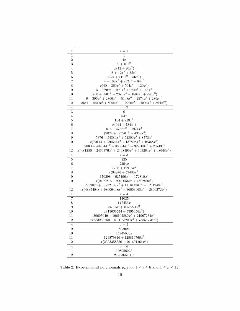
Since all of these conjectures have been experimentally motivated, we herebystart our recursion discussion in the historical spirit, with experimental resultsfirst (and knowing that some of the tabulated recursions in the present sectionare proven and some are not). We give our substantial evidence in Table 2,where cn,k (lowercase notation) is defined in (8), and in Table 3.
An example of our experimental forays runs as follows. The form of thenon-trivial coefficients for a possible recursion for the C3,k and C4,k was as-sisted by consulting Sloane’s Online Encyclopedia4 which for C4,k connectedthe coefficients to the sequence A063495.5 Having found these recursions, itwas then reasonable to assume the coefficients were polynomials of the conjec-tured degree; and the Tables were then built by numerical interpolation afterthe use of PSLQ. The predicted recursions were then numerically checked toextreme-precision at various values of k.
Table 2 shows recursions for the renormalized cn,k := k!n! 2−nCn,k, for1 ≤ n ≤ 12 and integer k. Using the recursion form (37) we end up withsimple (odd or even, positive) polynomials pn,i. The explicit polynomials pn,i
that we have found experimentally are shown in Tables 2 and 3.
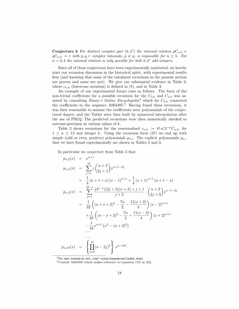
In particular we conjecture from Table 3 that
pn,0(x) = xn+1
pn,1(x) =M∑
j=1
j
(n + 22j + 1
)xn+1−2j
=14
(n + 1 + x) (x− 1)n+1 +14
(x + 1)n+1 (n + 1− x)
pn,2(x) =M−1∑j=1
j4j−1((2j + 3)(n + 2) + j + 1j + 2
·(
n + 22j + 3
)xn−1−2j
=132
((n + x + 2)2 − 7n
2− 11(x + 2)
4
)(x− 2)n+1
+132
((n− x + 2)2 − 7n
2+
11(x− 2)4
)(x + 2)n+1
− 116
xn+1(x2 − (n + 2)2
)· · ·· · ·
pn,M (x) =
M∏
j=0
(n− 2j)2
xn−2M .
4See www.research.att.com/∼njas/sequences/index.html.5Consult A063495 which makes reference to equation (10) in [24].
18
n i = 1
1 12 4x3 2 + 10x2
4 x(12 + 20x2)5 3 + 42x2 + 35x4
6 x(24 + 112x2 + 56x4)7 4 + 108x2 + 252x4 + 84x6
8 x(40 + 360x2 + 504x4 + 120x6)9 5 + 220x2 + 990x4 + 924x6 + 165x8
10 x(60 + 880x2 + 2376x4 + 1584x6 + 220x8)11 6 + 390x2 + 2860x4 + 5148x6 + 2574x8 + 286x10
12 x(84 + 1820x2 + 8008x4 + 10296x6 + 4004x8 + 364x10)
n i = 2
3 94 64x5 104 + 259x2
6 x(944 + 784x2)7 816 + 4752x2 + 1974x4
8 x(9024 + 17520x2 + 4368x4)9 5376 + 54384x2 + 52800x4 + 8778x6
10 x(70144 + 236544x2 + 137808x4 + 16368x6)11 32000 + 492544x2 + 830544x4 + 322608x6 + 28743x8
12 x(481280 + 2469376x2 + 2498496x4 + 693264x6 + 48048x8)
n i = 3
5 2256 2304x7 7796 + 12916x2
8 x(94976 + 52480x2)9 170298 + 625196x2 + 172810x4
10 x(2409216 + 2949056x2 + 489280x4)11 2999076 + 18232188x2 + 11161436x4 + 1234948x6
12 x(48354048 + 98000448x2 + 36003968x4 + 2846272x6)
n i = 4
7 110258 147456x9 851976 + 1057221x2
10 x(13036544 + 5395456x2)11 39605040 + 106102880x2 + 21967231x4
12 x(683253760 + 610355200x2 + 75851776x4)
n i = 5
9 89302510 14745600x11 129879846 + 128816766x2
12 x(2393358336 + 791691264x2)
n i = 6
11 10805602512 2123366400x
Table 2: Experimental polynomials pn,i for 1 ≤ i ≤ 6 and 1 ≤ n ≤ 12.
19
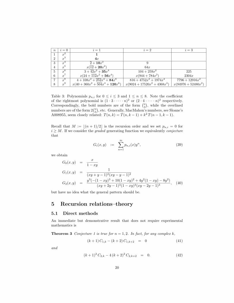
n i = 0 i = 1 i = 2 i = 3
1 x2 12 x3 4x
3 x4 2 + 10x2 94 x5 x(12 + 20x2) 64x
5 x6 3 + 42x2 + 35x4 104 + 259x2 2256 x7 x(24 + 112x2 + 56x4) x(944 + 784x2) 2304x
7 x8 4 + 108x2 + 252x4 + 84x6 816 + 4752x2 + 1974x4 7796 + 12916x2
8 x9 x(40 + 360x2 + 504x4 + 120x6) x(9024 + 17520x2 + 4368x4) x(94976 + 52480x2)
Table 3: Polynomials pn,i for 0 ≤ i ≤ 3 and 1 ≤ n ≤ 8. Note the coefficientof the rightmost polynomial is (1 · 3 · · · · · n)2 or (2 · 4 · · · · · n)2 respectively.Correspondingly, the bold numbers are of the form
(n3
), while the overlined
numbers are of the form 2(n5
), etc. Generally, MacMahon’s numbers, see Sloane’s
A008955, seem closely related: T (n, k) = T (n, k − 1) + k2 T (n− 1, k − 1).
Recall that M := b(n + 1)/2c is the recursion order and we set pn,i = 0 fori ≥ M . If we consider the graded generating function we equivalently conjecturethat
Gi(x, y) :=∞∑
n=1
pn,i(x)yn, (39)
we obtain
G0(x, y) =x
1− xy
G1(x, y) =1
(xy + y − 1)2(xy − y − 1)2
G2(x, y) =y3(−(1− xy)3 + 10(1− xy)2 + 4y2(1− xy)− 8y2)
(xy + 2y − 1)3(1− xy)3(xy − 2y − 1)3, (40)
but have no idea what the general pattern should be.
5 Recursion relations–theory
5.1 Direct methods
An immediate but demonstrative result that does not require experimentalmathematics is
Theorem 3 Conjecture 1 is true for n = 1, 2. In fact, for any complex k,
(k + 1) C1,k − (k + 2) C1,k+2 = 0 (41)
and
(k + 1)2 C2,k − 4 (k + 2)2 C2,k+2 = 0. (42)
20
Proof. The desired recursions follow immediately and analytically from (14)and (15) respectively. QED
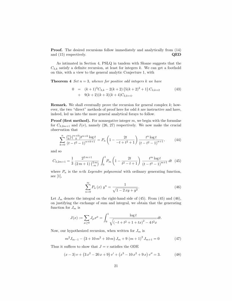
As intimated in Section 4, PSLQ in tandem with Sloane suggests that theC3,k satisfy a definite recursion, at least for integers k. We can get a footholdon this, with a view to the general analytic Conjecture 1, with
Theorem 4 Set n = 3, whence for positive odd integers k we have
0 = (k + 1)3C3,k − 2(k + 2)(5(k + 2)2 + 1
)C3,k+2 (43)
+ 9(k + 2)(k + 3)(k + 4)C3,k+4.
Remark. We shall eventually prove the recursion for general complex k; how-ever, the two “direct” methods of proof here for odd k are instructive and have,indeed, led us into the more general analytical forays to follow.
Proof (first method). For nonnegative integer m, we begin with the formulaefor C3,2m+1 and I(ν), namely (26, 27) respectively. We now make the crucialobservation that
n∑k=0
(nk
)(n+k
k
)tn+k log t
(t− t2 − 1)n+k+1= Pn
(1− 2t
−t + t2 + 1
)tn log t
(t− t2 − 1)n+1 , (44)
and so
C3,2m+1 =13
22 m+1
(2 m + 1)(2 mm
) ∫ 1
0
Pm
(1− 2t
t2 − t + 1
)tm log t
(t− t2 − 1)m+1 dt (45)
where Pn is the n-th Legendre polynomial with ordinary generating function,see [1],
∞∑n=0
Pn (x) yn =1√
1− 2 xy + y2. (46)
Let Jm denote the integral on the right-hand side of (45). From (45) and (46),on justifying the exchange of sum and integral, we obtain that the generatingfunction for Jm is
J(x) :=∑µ≥0
Jµxµ =∫ 1
0
log t√(−t + t2 + 1 + tx)2 − 4 t2x
dt.
Now, our hypothesized recursion, when written for Jm is
m2Jm−1 −(3 + 10 m2 + 10 m
)Jm + 9 (m + 1)2 Jm+1 = 0 (47)
Thus it suffices to show that J = v satisfies the ODE
(x− 3) v +(3 x2 − 20 x + 9
)v′ +
(x3 − 10 x2 + 9 x
)v′′ = 3. (48)
21

This is indeed the case. Maple easily confirms that the value of the left-handside of (48) is 3. QED
Proof (second method). Alternatively we observe that (26) writes C3,2m+1 =amJm where a (0) = 2/3 and
(−2 m− 2) a (m) + (2 m + 3) a (m + 1) = 0,
while Jm satisfies (47)—or via the proven recursion
(n + 1)2 u (n) + (n + 1) (2 n + 3)u (n + 1)− 3 (n + 2) (n + 1) u (n + 2) = −1,
for I. The INRIA-designed Maple package ‘gfun’ provides an algorithm whichwill then produce a recursion for C3,2n+1 which simplifies to the vanishing of
4 (m− 1)3 Jm−2−2 (2m− 1)(3 + 10 m2 − 10 m
)Jm−1+9 (2 m + 1) (2 m− 1) mJn
which Maple easily confirms to be as claimed. This proof also can be obtainedin Mathematica using Carsten Schneider’s ‘Sigma’ package available from Risc-Linz, [33]. Both programs can certify the result, for example in Mathematicausing ‘CreativeTelescoping’. QED
The coefficients Jm are interesting in their own right. In fact,
Jm = qmL−3(2)− pm →m 0
where for m ≥ 1
qm =12−
m−1∑k=1
9−k2F2
(12 ,−k,−k
1, 2 ; 4)
.
The first 6 values of pm and qm respectively are
(p0, . . . , p5) =13,
23108
,145972
,133111664
,2423532624400
,549550770858800
,
and(q0, . . . , q5) =
12,
518
,31162
,71486
,5174374
,11723118098
.
5.2 Analytic method
Presumably there are direct methods, analogous to those used for Theorem4, that would establish the experimentally motivated recursion for the C4,odd.However, it turns out that an analytic approach handles both C3,k and C4,k
recursions and moreover, does this for general complex k. Incidentally, by “gen-eral complex k” here and elsewhere, we mean either that Cn,k is defined as itsoriginal integral (1) and all k ∈ K are being considered, or we are contemplat-ing the analytic continuation Cn,k over the entire complex k-plane (and at polesrecursions still make divergent sense).
The following method of proof, relying on a contour-integral application ofthe Zeilberger algorithm [39, 12, 48], was suggested to us by W. Zudilin [50].
22

Theorem 5 The recursion in Theorem 4 for C3,odd k extends to complex k;moreover, there is a recursion of the same order (M = 2) for the C4,k. Explic-itly, both of the recursions
(k + 1)3C3,k − 2(k + 2)(5(k + 2)2 + 1
)C3,k+2 + 9(k + 2)(k + 3)(k + 4)C3,k+4
= 0,
(k + 1)4C4,k − 4(k + 2)2(5(k + 2)2 + 3)C4,k+2 + 64(k + 2)(k + 3)2(k + 4)C4,k+4
= 0,
hold for general complex k.
Proof. (i) We focus on the n = 4 case—the n = 3 case follows the same logic—using a representation based on the Meijer form (13) and its associated contourintegral. Contemplating t as a complex variable, we have
C4,2t−1 = − π2
24πi
∫ −1/2+i∞
−1/2−i∞F4(t, s)
cos πs
sin3 πsds,
with the definition
F4(t, s) :=Γ(s + 1/2)Γ(s + t)3
Γ(2t)Γ(s + 1)3Γ(1/2 + s + t).
If one then employs the Zeilberger algorithm6 one finds that the definition
G4(t, s) := s3 12t3 + 16t− 2 + 26st2 − 26t2 − 37ts + 11s + 18s2t + 4s3 − 12s2
(t− 1)(2s + 2t− 1)F4(t, s),
leads to
16t2(2t + 1)(2t− 1)F4(t + 1, s)− (2t− 1)2(5t2 − 5t + 2)F4(t, s)
+(t− 1)4F4(t− 1, s) = G4(t, s + 1)−G4(t, s).
Inserting this F,G relation into the contour integral yields
16t2(2t + 1)(2t− 1)C4,2t+1 − (2t− 1)2(5t2 − 5t + 2)C4,2t−1 + (t− 1)4C4,2t−3
=π2
24πi
ZC
G4(t, s)cos πs
sin3 πsds, (49)
where now the contour C is an infinitely tall, thin rectangle running verticallythrough −1/2 + 0i and 1/2 + 0i.
However, this rectangular integral is zero, since the only singularity is ats = 0, and as we saw in our previous Meijer analysis for C4,k, the residuecontribution is proportional to ∂2G4(t, s)/∂s2|s=0, which is zero. Thus, therecursion (49) holds in an analytic sense, and upon t → (k + 3)/2 becomes theorder-2 recursion desired.
6Say, by calling in Maple zeil(F4(t-1,s),s,t,N,2).
23

(ii) For n = 3, the same procedure goes through; we first harken back toMeijer representation (12) then define
F3(t, s) :=Γ(s + 1/2)Γ(s + t)2
Γ(2t)Γ(s + 1)3,
then run the Zeilberger algorithm to achieve
G3(t, s) := s3 12t3 − 17t2 + 14st2 − 10st + 6t + 4s2t− s2 + 2s− 12t(t− 1)
F3(t, s)
and
(4t + 1)(2t + 1)(2t− 1)(4t− 1)F3(t + 1, s)− t(2t− 1)(10t2 − 10t + 3)F3(t, s)
+t(t− 1)3F3(t− 1, s) = G3(t, s + 1)−G3(t, s).
Then, as with the n = 4 case above, we observe the vanishing of the relevantcontour integral and arrive at the correct recursion involving C3,2t−1. QED
6 Continued fractions
It will have occurred to many readers that the order M = 2 recurrences, namelyfor the C3,k and C4,k, should give rise to continued fractions, being as such frac-tions are also governed by order-2 recurrences. The classical Pincherle theorem[23, Theorem 7, p.202], [19] runs like so:
Theorem 6 (Pincherle) Let (aN : N ∈ Z+), (bN : N ∈ Z+), (GN : N =−1, 0, 1, 2, . . . ) be sequences of complex numbers related for all N ∈ Z+ by
GN = bNGN−1 + aNGN−2,
with each aN 6= 0. Denote by PN/QN the convergents to the continued fraction
x :=a1
b1 + a2b2+...
.
If limN GN/QN = 0 then the fraction converges and has the value
x = − G0
G−1.
The Pincherle theorem may be applied to recursions of the form in Conjecture1 when n = 3 or 4, as established in Theorem 5. For these n we have order-2recursions:
Pn,0(k)Cn,k + Pn,1(k)Cn,k+2 + Pn,2(k)Cn,k+4 = 0.
24

If we identify GN := Cn,2N+2 the Pincherle theorem applies with
bN := −Pn,1(2N − 2)Pn,2(2N − 2)
,
aN := −Pn,0(2N − 2)Pn,2(2N − 2)
,
and we obtain a continued fraction with value x = −Cn,2/Cn,0. Similarly,setting GN := Cn,2N+3 and suitably modifying the definitions of aN , bN givesus a fraction with value −Cn,3/Cn,1.
These machinations result in at least four attractive continued fractions hav-ing integer elements. Even though we do not know a single individual value ofC3,even, we nevertheless have a fraction for the ratio C3,2/C3,0; specifically,
18C3,2
C3,0=
9 · 14
d(1)−9 · 34
. . . −9 · (2N − 1)4
d(N)− . . .
(50)
where d(N) := 40N2 + 2. The very form of the fraction elements suggests thatthis ratio could well be a rational multiple of some brand of L-function, but wehave not extensively searched for such.
For the L-function that appears in C3,odd evaluations, we obtain
2L−3(2)
= 3−9 · 14
f(1)−9 · 24
. . . −9 ·N4
f(N)− . . .
(51)
with f(N) := 10N2 + 10N + 3, and so f(0) = 3.Along the same lines one derives a fraction
16C4,2
C4,0=
16
e(1)−36
. . . −(2N − 1)6
e(N)− . . .
(52)
where e(N) := N(20N2 + 3).Finally, for the C4,odd we arrive at a fraction for ζ(3):
127 ζ(3)
= 2−16 · 16
g(1)−16 · 26
. . . −16 ·N6
g(N)− · · ·
, (53)
25

where g(N) := (2N + 1)(5N2 + 5N + 2), and so g(0) = 2. This fraction isstructurally reminiscent of the Apery continued fraction for ζ(3). (See [17] andthe references therein.) However, the arguments presented in [44]—where arederived Catalan-constant and ζ(4) fractions structurally similar to our L andζ(3) fractions above—suggest that irrationality proofs using such fractions arerare. Typically, certain number-theoretical properties of a recursion must besatisfied for an irrationality proof to be achievable.
Indeed there are many literature connections involving recursions, continuedfractions, and irrationality [5, 26, 45, 31, 38, 46, 48]. Indeed, our recursion forC4,k in Theorem 5 (essentially a recursion relevant to ζ(3)) can be found in theliterature [4, p.23], and another one for the C3,k, and so relevant to L−3(2) canbe found also [49]. We note that irrationality proofs of Apery type do not appearto arise from the recursions of the present paper. Indeed, to our knowledge thenumber L−3(2) has never been proven irrational.
7 Further analytic properties of the Cn,k
We have investigated interindicial relations of k-variant form, i.e. recursionrelations, but now we turn to relations where the first index, n, varies.
7.1 Analytic convolution
On another idea of W. Zudilin [50], we sought relations on the first index,namely the n of Cn,k. One result is an analytic convolution theorem, where werecall the definition of the half-plane K from Section 1, and the renormalizationcn,k := Γ(k + 1)2−nn! Cn,k:
Theorem 7 For complex k ∈ K, positive integer n, and integer q ∈ [1, n − 1]we have
cn,k =1
2πi
∫C
cn−q,k+scq,−1−s ds,
where the contour C runs vertically over (λ− i∞, λ + i∞) with <(λ) ∈ (−1, 0).
Remark. There are at least two remarkable features of this result. First,this is a kind of recursion on the first index of the cn,k in contrast with thek-recursions; and second, the convolution surprisingly takes the same form forany (legal) indicial offset q.
Proof. Write our original definition (1) in the form
Cn,k :=1n!
∫dx1 · · · dxn(A + B)−k−1 =
1n!
∫dx1 · · · dxnA−k−1(1 + B/A)−k−1
where A is the sum of the first (n − q) cosh terms, and B is the sum of theremaining q cosh terms. We then invoke the hypergeometric form of the binomial
26
theorem, namely
(1 + B/A)−k−1 =1
Γ(k + 1)1
2πi
∫C
Γ(1 + k + s)Γ(−s)(B/A)s ds.
We can then contemplate integration of A terms over dx1 · · · dxn−q, and B termsover dxn−q+1 · · · dxn, to obtain
Cn,k =1(nq
) 1Γ(k + 1)
12πi
∫C
Γ(k + 1 + s)Γ(−s)Cn−q,k+sCq,−1−s ds.
But upon renormalization to the little-c forms, this is the statement of thetheorem. QED
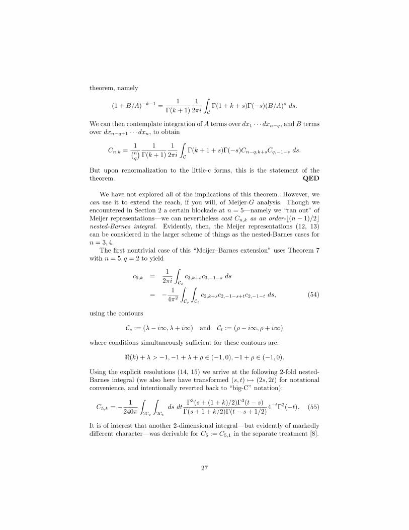
We have not explored all of the implications of this theorem. However, wecan use it to extend the reach, if you will, of Meijer-G analysis. Though weencountered in Section 2 a certain blockade at n = 5—namely we “ran out” ofMeijer representations—we can nevertheless cast Cn,k as an order-b(n − 1)/2cnested-Barnes integral. Evidently, then, the Meijer representations (12, 13)can be considered in the larger scheme of things as the nested-Barnes cases forn = 3, 4.
The first nontrivial case of this “Meijer–Barnes extension” uses Theorem 7with n = 5, q = 2 to yield
c5,k =1
2πi
∫Cs
c2,k+sc3,−1−s ds
= − 14π2
∫Cs
∫Ct
c2,k+sc2,−1−s+tc2,−1−t ds, (54)
using the contours
Cs := (λ− i∞, λ + i∞) and Ct := (ρ− i∞, ρ + i∞)
where conditions simultaneously sufficient for these contours are:
<(k) + λ > −1,−1 + λ + ρ ∈ (−1, 0),−1 + ρ ∈ (−1, 0).
Using the explicit resolutions (14, 15) we arrive at the following 2-fold nested-Barnes integral (we also here have transformed (s, t) 7→ (2s, 2t) for notationalconvenience, and intentionally reverted back to “big-C” notation):
C5,k = − 1240π
∫2Cs
∫2Ct
ds dtΓ3(s + (1 + k)/2)Γ3(t− s)
Γ(s + 1 + k/2)Γ(t− s + 1/2)4−tΓ2(−t). (55)
It is of interest that another 2-dimensional integral—but evidently of markedlydifferent character—was derivable for C5 := C5,1 in the separate treatment [8].
27

7.2 Measure-theoretic representation
Again starting from the original definition (1) we denote the sum of cosh termsas U , and develop a measure-theoretic form:
Cn,k =1n!
∫ ∞
n
dU
Uk+1
∂
∂U
∫P
cosh xk≤U
dx1 · · · dxn,
or, upon integration by parts,
Cn,k =k + 1
n!2n+2
∫ ∞
0
r Vn(r)(2r2 + n)k+2
dr,
where the volume Vn is that of a “hyper-ellipsoid” of “radius” r:
Vn(r) :=∫P
sinh2 yk≤r2dy1 · · · dyn. (56)
A test case is n = 1, for which V1(r) = 2 arcsinh r, and this measure-theoreticform agrees with (14).
This approach has not been taken further; however, note that we alwayshave a 1-dimensional integral, for any n—an advantage shared by the Bessel-kernel representations. In the measure-theoretic case here, though, all involvedfunctions are elementary. It is also interesting that if we had omniscience inregard to the properties of the hyper-ellipsoid, we would settle many questionsabout the Cn,k.
7.3 An n-variant recursion and the elusive C5
Presumably the convolution Theorem 7 could be invoked, the resulting residuecalculus giving us relations between the cn,k and entities cp,j with p < n. How-ever there is a much more direct way to establish an n-variant recursion (i.e.,now we have the first index n changing on cn,k). The Bessel-kernel representa-tion (7) together with the insertion of one copy of K0 in the form of an ascendingseries
K(asc)0 (t) =
∑k≥0
t2k
4kk!2{Hk − γ − log(t/2)} , (57)
see [1, 8], immediately yields an n-variant recursion (recall cn,k := Γ(k +1)2−nn!Cn,k):
cn,k =∑m≥0
14m
1m!2
{(H(1)
m − γ + log 2) cn−1,k+2m − c′n−1,k+2m
}, (58)
where the derivative is with respect to the second index, i.e. c′n,q := ∂cn,q/∂q.Interestingly, for the problematic Ising integral C5 := C5,1 = c5,1/450, we ac-tually know all of the c4,2m+1 in principle, from Theorem 2 and the resultingalgorithm. Unfortunately we still do not have a convenient representation forc′4,2m+1, but at least we have derived a computational series involving, say,numerical differentiation, for C5.
28

7.4 Bessel-moment relation
Using an integration by parts, namely
1Γ(k + 1)
∫ ∞
0
tkKn0 (t) dt =
1Γ(k + 3)
∫ ∞
0
tk+2 (Kn0 (t))′′ dt
in the original definition (1), we can iterate in view of the recursion Conjecture 1to write an equivalent conjecture as a Bessel-moment phenomenon—with M :=b(n + 1)/2c as in the conjecture:
0 ?=∫ ∞
0
tk+2M(PM (k)Kn
0 + PM−1(k)(Kn0 )′′ + · · ·+ P0(k)(Kn
0 )(2M))
dt.
It is remarkable that polynomials P0, . . . , PM exist such that this moment in-tegral appears to vanish for general complex k ∈ K (of course, the equivalentrecursion relations are likewise remarkable). Note that the suspected vanishingof the above moment integral has been proven for n = 1, 2, 3, 4 and appropriaterespective polynomials.
We have not taken this moment relation any further than to make the fol-lowing observation. Using the asymptotic series [1]:
K(asy)0 (t) ∼
√π
2te−t
∞∑m=0
(−1)m((2m)!)2
m!3(32t)m, (59)
one may ask how the Bessel-moment integral above behaves when the asymp-totic form is (naively, perhaps illegally) simply inserted into the integral. Sur-prisingly, if one truncates the sum (59) at a high enough m, and solves for thepolynomials that minimize the k-degree of the moment integral, one evidentlyfinds the correct polynomials exactly.
For example, we took the summation index m up through 18, and solvedsymbolically for the higher powers of k in the moment integral’s result to vanish,and found we had detected this relation (36) previously, numerically, so it waspleasing to find the same polynomials via this admittedly nonrigorous handlingof the moment integral. The fascinating nuance here is that, evidently, therecursion polynomials depend in some profound sense on the coefficients of theasymptotic expansion in (59).
8 Extreme-precision numerics
Using the Bessel-kernel representation (7), we have calculated to 500-digit ac-curacy values of Cn,k for all integers n, k, where n ∈ [2, 12] and k ∈ [0, 25]. Thiswas done using the ARPREC arbitrary precision software [10] and the tanh-sinhquadrature scheme [11]. We have placed a listing of these numerical values ona website [9]. These were the raw data on which most of our discoveries werebased.
29

9 Conclusion and open problems
We wish to emphasize that the interaction of sophisticated numeric and sym-bolic computing has played an irreplaceable role in the work described herein.Indeed, we believe that these results would have been much more difficult,if not impossible, to deduce without reliance on heavy-duty computer powerand sophisticated algorithms. Some of the techniques we employed includeextreme-precision quadrature, PSLQ integer relation detection programs, gen-erating function packages, high-accuracy least-squares polynomial fitting, andWilf–Zeilberger theorem-proving software. We wish to thank those who haveprovided both the hardware and the software we have used.
We finish by recording some of the open problems we find the most com-pelling.
• While Conjectures 2 and 3 are probably out of current reach, what progressis possible on Conjecture 1. Specifically:
• How might one prove the conjectured recursion for n = 5, from (35),using, say, the nested-Barnes representation (55)? This might amount toa higher-dimensional application of Wilf–Zeilberger methods [39].
• Is there a reasonable closed form for some or all of the following constants:C5,1, C4,0, C3,2/C3,0, C4,2/C4,0?
Acknowledgments. We are indebted to V. Adamchik, P. Paule, C. Schneider,P. Wellin, and A. van der Poorten. We give special acknowledgment to toW. Zudilin whose advice and expertise in various aspects of this research wereindispensable.
References
[1] Milton Abramowitz and Irene A. Stegun, Handbook of Mathematical Functions,Dover, NY, 1970.
[2] V. Adamchik, “The evaluation of integrals of Bessel functions via G-functionidentities.” Journal of Computational and Applied Mathematics, 64 (1995),283–290.
[3] V. Adamchik, Private communication, Mar 2006.
[4] G. Almkvist and W. Zudilin, “Differential equations, mirror maps and zetavalues,” E-printmath.NT/0402386, 2004.
[5] R. Apery, “Irrationalite de ζ(2) et ζ(3),” Asterisque 61, (1979), 11–13.
[6] David H. Bailey and Jonathan M. Borwein, “Highly parallel, high-precisionnumerical integration,” D-drive Preprint #294, 2005. Also available athttp://crd.lbl.gov/~dhbailey/dhbpapers/quadparallel.pdf.
30
[7] David H. Bailey and Jonathan M. Borwein, “Effective error bounds forEuler-Maclaurin-based quadrature schemes,” D-drive Preprint #297, 2005. Alsoavailable at http://crd.lbl.gov/~dhbailey/dhbpapers/em-error.pdf.
[8] David H. Bailey, Jonathan M. Borwein and Richard E. Crandall, “Integrals ofthe Ising class,” J. Phys. A.: Math. Gen., to appear (2007). Also, D-drivePreprint #324, 2006, andhttp://crd.lbl.gov/~dhbailey/dhbpapers/ising.pdf.
[9] David H. Bailey, Jonathan M. Borwein and Richard E. Crandall, “Ising data,”available at http://crd.lbl.gov/~dhbailey/dhbpapers/ising-data.pdf.
[10] David H. Bailey, Yozo Hida, Xiaoye S. Li and Brandon Thompson, “ARPREC:An Arbitrary Precision Computation Package,” 2002, available athttp://crd.lbl.gov/ dhbailey/dhbpapers/arprec.pdf.
[11] David H. Bailey, Xiaoye S. Li and Karthik Jeyabalan, “A comparison of threehigh-precision quadrature schemes,” Experimental Mathematics, 14 (2005),317–329.
[12] A. Becirovic et al., “Hypergeometric summation algorithms for high-order finiteelements,” Johann Kepler University, Linz. Technical Report #2006–8.
[13] H. E. Boos and V. E. Korepin, “Quantum spin chains and Riemann zetafunction with odd argument,” Preprint, available athttp://www.arxiv.org/hep-th/0104008, 2001.
[14] J.M. Borwein, “Hilbert Inequalities and Witten Zeta-functions,” D-drivePreprint #309, 2005.
[15] Jonathan M. Borwein and David H. Bailey, Mathematics by Experiment, AKPeters, 2003.
[16] Jonathan M. Borwein, David H. Bailey and Roland Girgensohn,Experimentation in Mathematics, AK Peters, 2004.
[17] Jonathan M. Borwein, David M. Bradley and Richard E. Crandall,“Computational strategies for the Riemann zeta function,” Journal ofComputational and Applied Mathematics, special volume “Numerical Analysisin the 20th Century. Vol. 1: Approximation Theory.” 121 (2000), 247–296[CECM Preprint 98:118].
[18] Jonathan M. Borwein and Peter B. Borwein, Pi and the AGM, John Wiley,1987.
[19] D. Bowman and J. McLaughlin, “Polynomial continued fractions,” ActaArithmetica, 103 (2002), 329–342.
[20] P. Flajolet et al., “On the non-holonomic character of logarithms, powers, andthe n-th prime function,” Electronic Journal of Combinatorics, 11, #A00, 2005.
[21] Frances Y. Kuo and Ian H. Sloan, “Lifting the curse of dimensionality,” Noticesof the AMS, 52, no. 11, (2005), 1320–1329.
31
[22] L. Lewin, Polylogarithms and Associated Functions, North Holland, 1981.
[23] L. Lorentzen and H. Waadeland, Continued Fractions with Applications,North-Holland, Amsterdam, 1992.
[24] T. P. Martin, “Shells of Atoms,” Phys. Reports, 273 (1996), 199–241.
[25] J-M. Maillard, Private communication, January 2005.
[26] J. McLaughlin and N. Wyshinski,“Real numbers with polynomial continuedfraction expansions,” Manuscript, 2004.
[27] B. Nickel, “On the singularity structure of the 2D Ising model susceptibility,”Journal of Physics A: Mathematics and General, 32 (1999), 3889–3906.
[28] F. Oberhettinger, Tables of Fourier Transforms and Fourier Transforms ofDistributions, Springer-Verlag, 1990.
[29] W. Orrick, B. Nickel, A. Guttmann, and J. Perk, “The susceptibility of thesquare lattice Ising model: New developments,” Manuscript, March 2001.
[30] J. Palmer and C. Tracy, “Two-dimensional Ising correlations: Convergence ofthe scaling limit,” Advances in Applied Mathematics, 2 (1981), 329-388.
[31] M. Prevost, “A new proof of the irrationality of ζ(2) and ζ(3) using Padeapproximants,” Journal of Computational and Applied Mathematics, 67 (1996),219–235.
[32] K. Roach, “Meijer G-function representations,” Proceedings of the 1997International Symposium on Symbolic and Algebraic Computation, 205–211,New York, ACM, 1997.
[33] C. Schneider, Private communication, July 2006.
[34] C. A. Tracy, “Painleve transcendents and scaling functions of thetwo-dimensional Ising model,” in Nonlinear Equations in Physics andMathematics, ed. A. O. Barut, D. Reidel Publ. Co., Dordrecht, Holland, (1978),378–380.
[35] C. Tracy, Private communication, Oct-Jan 2005.
[36] C. Tracy, Unpublished notes, 1976.
[37] A. J. van der Poorten and I. E. Shparlinski, “On linear recurrence sequenceswith polynomial coefficients,” Manuscript, 2005.
[38] A. J. van der Poorten, “A proof that Euler missed: Apery’s proof of theirrationality of ζ(3),” Mathematics Intelligencer, 1, no. 4 (1978/79), 195–203.
[39] H. Wilf and D. Zeilberger, “An algorithmic proof theory for hypergeometric(ordinary and “q”) multisum/integral identities,” Inventiones Mathematicae108, 575–63, 1992.
[40] T. T. Wu, B. M. McCoy, C. A. Tracy and E. Barouch, “Spin-spin correlationfunctions for the two-dimensional Ising model: Exact theory in the scalingregion,” Physical Review B13 (1976), 316-374.
32

[41] N. Zenine, S. Boukraa, S. Hassani and J-M Maillard, “Square lattice Isingsusceptibility: Connection matrices and singular behaviour of χ(3) and χ(4),”Journal of Physics A: Mathematical and General 38 (2005), 9439-9474.
[42] N. Zenine, S. Boukraa, S. Hassani and J-M Maillard, “Beyond series expansions:Mathematical structures for the susceptibility of the square lattice Ising model,”J. Physics Conference (electronic review of J. Physics), to appear, June 2006.
[43] N. Zenine, S. Boukraa, S. Hassani and J-M Maillard, “Differential Galois groupsof high order Fuchsian ODEs,” Preprint, 2005.
[44] W. Zudilin, “An Apery-like difference equation for Catalan’s constant,”Electronic Journal of Combinatorics 2003, #R14, 1–10.
[45] W. Zudilin, “A third-order Apery-like recursion for ζ(5),” Preprint, available athttp://www.arxiv.org/abs/math.NT/0206178, 2002.
[46] W. Zudlin, “An elementary proof of Apery’s theorem,” Preprint, available athttp://www.arxiv.org/math.NT/0202159, 2002.
[47] V. Zudilin, “Difference equations and the irrationality measure of numbers,”Proceedings of the Steklov Institute of Mathematics, 218 (1997), 160–174.
[48] V. Zudilin, “Approximations to di- and tri-logarithms,” Preprint, available athttp://www.arxiv.org/math.NT/0409023, 2004.
[49] W. Zudilin, “Well-poised generation of Apery-like recursions, Preprint, availableat http://www.arxiv.org/math.NT/0307058, 2003.
[50] V. Zudilin, Private communication.
33