Embed Size (px)
Citation preview
HYDROLOGICAL PROCESSESHydrol. Process. 16, 1-26 (2002)DOI: 10.1002/hyp.273
A simple model of river meandering and its comparison to natural channels
Stephen T. Lancaster1* and Rafael L. Bras2
1Department of Geosciences, Oregon State University, Corvallis, OR, 97331, USA2Department of Civil and Environmental Engineering, Massachusetts Institute of Technology, Cambridge, MA 02139, USA
Abstract:We develop a new method for analysis of meandering channels based on planform sinuosity. This analysis objectivelyidentifies three channel reach lengths based on sinuosity measured at those lengths: the length of typical, simple bends;the length of long, often compound bends; and the length of several bends in sequence that often evolve from compoundbends to form multi-bend loops. These lengths, when normalized by channel width, tend to fall into distinct and clus-tered ranges for different natural channels. Mean sinuosity at these lengths also falls into distinct ranges. That range islargest for the third and greatest length, indicating that, for some streams, multi-bend loops are important for planformsinuosity while, for other streams, multi-bend loops are less important. The role of multi-bend loops is seldom addressedin the literature, and they are not well predicted by previous modeling efforts. Also neglected by previous modelingefforts is bank-flow interaction and its role in meander evolution. We introduce a simple river meandering model basedon topographic steering that has more in common with cellular approaches to channel braiding and landscape evolutionmodeling than to rigorous, physics-based analyses of river meandering. The model is sufficient to produce reasonablemeandering channel evolution and predicts compound bend and multi-bend loop formation similar to that observed innature in both mechanism and importance for planform sinuosity. In the model, the tendency to form compound bends issensitive to the relative magnitudes of two lengths governing meander evolution: (i) the distance between the bendcross-over and the zone of maximum bank shear stress, and (ii) the bank shear stress dissipation length related to bankroughness. In our simple model, the two lengths are independent. This sensitivity implies that the tendency for naturalchannels to form compound bends may be greater when the banks are smoother. Copyright © 2002 John Wiley & Sons,Ltd.
KEY WORDS fluvial geomorphology; river meandering
INTRODUCTION
River meandering is a complicated process involving the interaction of flow through channel bends, bankerosion, and sediment transport. Some aspects of this process are better understood than others. Studies atthe spatial scale of one to several bends (bend scale) and times that are short relative to the time from bendinception to cut-off (bend lifetime) are relatively numerous and have led to a detailed understanding of flowthrough channel bends and the interaction between that flow and the bed (e.g., Johannesson and Parker,1989a,b,c; Smith and McLean, 1984; Nelson and Smith, 1989a,b; Blondeaux and Seminara, 1985; Seminaraand Tubino, 1989, 1992; Imran et al., 1999). The previous studies did not address the interaction between theflow and the bank, the interaction that produces bank shear stress and bank erosion. Thorne and Osman(1988) did study the effect of bank stability on bed form and, thus, one effect of the bank on the flow, butThorne and Furbish (1995) showed that bank roughness affects the flow field and its interaction with thebank. Nelson and Smith (1989b) noted that consideration of lateral boundary effects would be necessary toextend their model to simulation of meandering.
*Correspondence to: S.T. Lancaster, Department of Geosciences, Oregon State University, 3200 SW Jefferson Way, Corvallis, OR, 97331,USA. E-mail: [email protected]
Received 30 May 2000Copyright © 2002 John Wiley & Sons, Ltd. Accepted 17 January 2001
2 S.T. LANCASTER AND R.L. BRAS
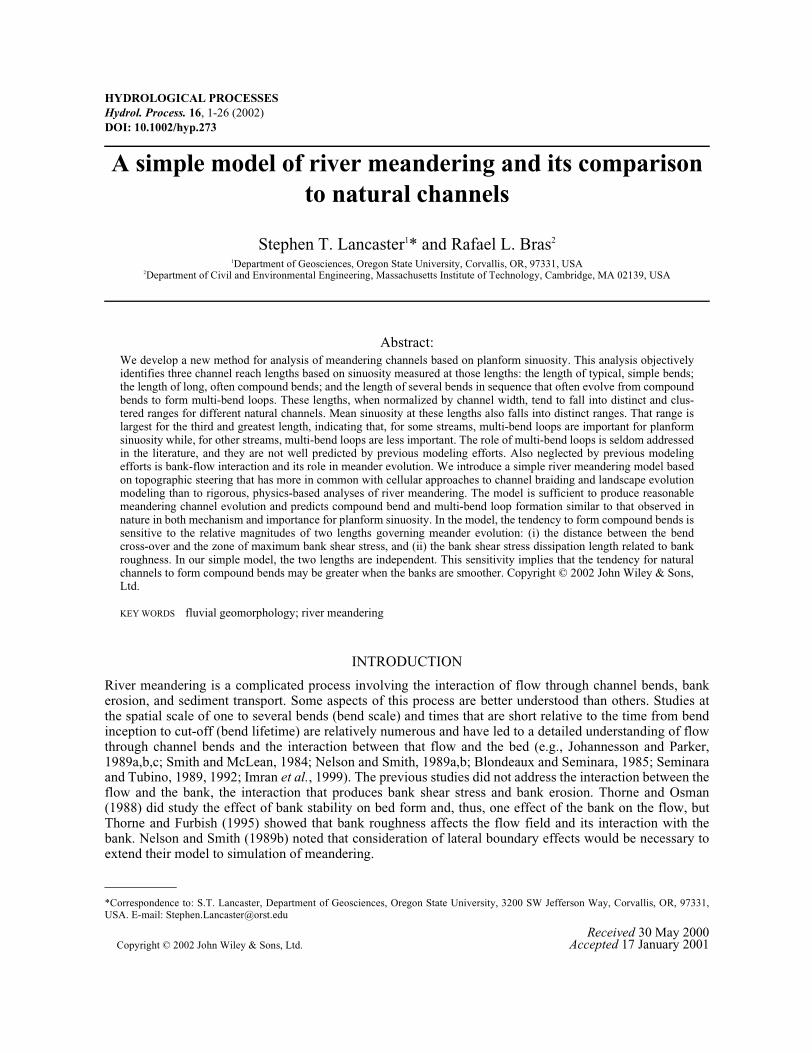
Another relatively poorly understood aspect of meandering is channel planform complexity. Meanderingproduces channel planforms that are relatively simple and recognizable at the bend scale but relatively com-plex and baffling at the scale of many, e.g., 100, bends (reach scale). A major contributor to planform com-plexity is compound bend formation, i.e., the “cumuliform” shapes noted by Howard (1992), the “compoundbends” observed by Brice (1974), and the “lobing” and “double heading” studied by Hooke and Harvey(1983) among others. We define compound bends as bends that evolve from simple bends to develop a cur-vature reversal in the course of the bend (Figure 1). Brice (1974) showed with successive aerial photographsof the White River, IN, that a compound bend evolved from a simple bend following rapid downstreammigration of the upstream bend. Our own analysis of aerial photography of the Ellis River, ME, shows thismechanism for two compound bends (Figure 1). Compound bends often lead to bend separation and the for-mation of larger cumuliform shapes, i.e., multi-bend loops (Figure 1), and Hooke and Harvey (1983) stated,“[Compound bend formation] is the major process whereby new bends develop.”
A new measure of channel planforms, developed herein, shows that the phenomenon of compound bendand multi-bend loop formation (i) occurs at characteristic channel length-scales, (ii) adds secondary and ter-tiary sinuosity to the planform, and (iii) varies in its importance among different streams.
Previous studies have reached different conclusions regarding the mechanism for compound bend forma-tion. Hooke and Harvey (1983) and Thompson (1986) both asserted that a single pool-riffle unit cannot be
(a)
(b)
*
*
#
100 m
#
Figure 1. Examples of channel planforms and evolution at two locations, (a) and (b), on the Ellis River in Maine. Channels were extractedfrom aerial photographs and superimposed; light gray is 1943, dark gray is 1965, and black is 1992; flow is from left to right. In (a) aseries of simple bends and one compound bend (*) form a multi-bend loop (between # symbols). In (a) and (b) the time sequence showscompound bend formation. In both cases, cut-off of an upstream bend and a subsequent ‘wave’ of rapid downstream migration lead tocurvature reversal at (*), where curvature was low before the cut-off occurred. Field reconnaissance at site (a) confirmed that the bankmaterial is homogeneous
Copyright © 2002 John Wiley & Sons, Ltd. Hydrol. Process. 16, 1-26 (2002)
MODEL FOR RIVER MEANDERING 3
sustained in longer bends but disagreed on the mechanism for subdivision of pools by new riffles, the formerattributing it to the non-sustainability of the necessary secondary flows and the latter to the kinematics ofsediment transport. Both studies concluded that the formation of new pool-riffle sequences preceded, andcaused, compound bend formation. Ferguson (1984) found that compound bends could be the result ofdecreasing migration rate with curvature greater than some threshold, as observed by Nanson and Hickin(1983), but the physical mechanism for this decrease is uncertain. Furthermore, Furbish (1988) shows thatthe same data confirm that migration rate increases monotonically with curvature when bend length isaccounted for, and Furbish (1991) concludes that there is no preferred, shorter bend length except in rarecases when the transverse bed slope is unusually small. This result would imply, however, that compoundbend formation is rare, contrary to the observations of many authors including those cited above.
Previous physically based models, in their simplest forms, do not reproduce compound bends or cumuli-form shapes. Sun et al. (1996) invoked heterogeneity of bank erodibility to explain cumuliform shapes. Theyran the Johannesson and Parker (1989a) model with an uncorrellated random field of heterogeneous bankerodibility and produced something like compound bends, but these bend shapes did not evolve from simplebends by the mechanism observed by Brice (1974) and shown in Figure 1. Tao Sun and others (T. Sun, per-sonal communication, 2000) have recently modeled meandering near the resonance between forced andalternate bars to produce long bends that divide into smaller ones, but the simulated phenomenon lacks thedouble heading characteristic of most compound bend formation and noted by previous authors.
We hypothesize that this phenomenon emerges from first-order, inherent dynamics, particularly from theinteractions between the flow and banks. A field study by Thorne and Furbish (1995) showed that removingthe roughness of natural banks has a large and measurable effect on the dynamics of the high-velocity coreof the flow in the channel. The interaction between the core and the bank produces the shear stress thaterodes the bank. Previous modelers have often made the simplifying assumption that bank shear stress isproportional to the near-bank downstream velocity perturbation but have found the problem of the bank’sinfluence, in turn, on the near-bank, shear stress-producing flow intractable (e.g., Johannesson and Parker,1989a; Smith and McLean, 1984; Nelson and Smith, 1989b). We address this issue with a simple conceptualmodel.
The complicated processes of channel and landscape evolution are commonly represented by simple mod-els that are based on both the process physics and a set of rules. For example, the cellular braided-streammodel of Murray and Paola (1994, 1997), the alluvial basin model of Paola et al. (1992), and the landscapeevolution models developed by many authors, e.g., Willgoose et al. (1991), Howard (1994), and Tucker andSlingerland (1994), all combine physics and rules to describe complex systems. A main objective of suchmodeling is to enhance our understanding of natural phenomena rather than to develop fully descriptive the-ories.
In this paper, we develop a simple model of river meandering that also combines physics and rules. It isbased on the concept of topographic steering (Dietrich and Smith, 1983). The model treats the flow’s inter-action with the bank through an independent, adjustable parameter and is sufficient to produce realisticmeandering (i.e., it provides “sufficient conditions for meandering” as in Howard and Knutson (1984)). Wejustify the model with this sufficiency. Our goal is to simulate realistic meandering over times appropriatefor landscape evolution, not to perform a rigorous, physical derivation. The model produces cumuliformshapes and compound bends without invoking heterogeneity or other second-order effects.
MODEL
In nearly all models of meander migration, local migration depends on upstream conditions, usually plan-form curvature. This is true of both the kinematic models of, e.g., Beck (1984), Ferguson (1984), Howardand Knutson (1984), and Furbish (1991) and the physical models of, e.g., Johannesson and Parker (1985,1989a,b,c). In the model presented here, local migration also depends on upstream conditions, but here thatcondition is the shoaling driven by changing bed topography and, ultimately, changing planform curvature.
Copyright © 2002 John Wiley & Sons, Ltd. Hydrol. Process. 16, 1-26 (2002)
4 S.T. LANCASTER AND R.L. BRAS
Also as in previous models, we assume that migration is equivalent to bank erosion on one side of the chan-nel, i.e., that deposition “keeps up” with erosion.
Field studies have shown that the primary downstream current erodes the bank when the flow’s highvelocity core nears the bank (e.g., Hasegawa, 1989; Pizzuto and Meckelnburg, 1989). Secondary flows“steer” the high velocity core by effecting a lateral transfer of downstream momentum. Dietrich and Smith(1983) found in a natural channel that the largest lateral transfer of downstream momentum was related tobed topography and called this phenomenon “topographic steering”. Smith and McLean (1984) showed ana-lytically that topographic steering terms in the momentum equations were too large to be treated as perturba-tions, in contrast to Johannesson and Parker (1989a,b,c), who treated all secondary flows as perturbations onthe mean behaviour. Our river meandering model is based on a simplified representation of the topographicsteering mechanism.
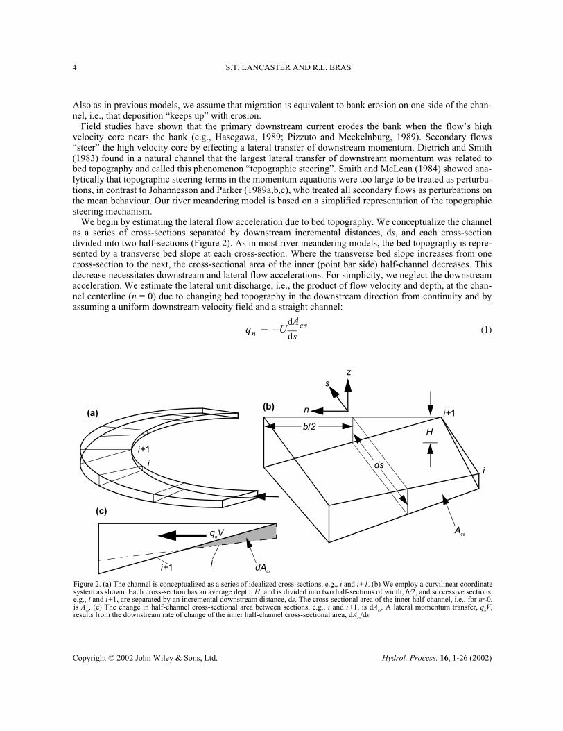
We begin by estimating the lateral flow acceleration due to bed topography. We conceptualize the channelas a series of cross-sections separated by downstream incremental distances, ds, and each cross-sectiondivided into two half-sections (Figure 2). As in most river meandering models, the bed topography is repre-sented by a transverse bed slope at each cross-section. Where the transverse bed slope increases from onecross-section to the next, the cross-sectional area of the inner (point bar side) half-channel decreases. Thisdecrease necessitates downstream and lateral flow accelerations. For simplicity, we neglect the downstreamacceleration. We estimate the lateral unit discharge, i.e., the product of flow velocity and depth, at the chan-nel centerline (n = 0) due to changing bed topography in the downstream direction from continuity and byassuming a uniform downstream velocity field and a straight channel:
(1)qn Usd
dAcs–=
Figure 2. (a) The channel is conceptualized as a series of idealized cross-sections, e.g., i and i+1. (b) We employ a curvilinear coordinatesystem as shown. Each cross-section has an average depth, H, and is divided into two half-sections of width, b/2, and successive sections,e.g., i and i+1, are separated by an incremental downstream distance, ds. The cross-sectional area of the inner half-channel, i.e., for n<0,is Acs. (c) The change in half-channel cross-sectional area between sections, e.g., i and i+1, is dAcs. A lateral momentum transfer, qnV,results from the downstream rate of change of the inner half-channel cross-sectional area, dAcs/ds
s
n
z
(a)
dAcs
(c)
H
ds
b/2
qnV
i
i+1
i+1
i
ii+1
Acs
(b)
Copyright © 2002 John Wiley & Sons, Ltd. Hydrol. Process. 16, 1-26 (2002)
MODEL FOR RIVER MEANDERING 5
where U is the average downstream flow velocity (downstream discharge and channel width are constantand given as input parameters; downstream velocity and flow depth are determined by continuity and theManning equation); and Acs is the inner half-channel (n < 0) cross-sectional area (Figure 2). In calculating Acs,we assume that lateral and downstream variations in free surface elevation are negligible relative to lateraland downstream variations in bed elevation. Field data support this assumption (e.g., Dietrich and Whiting,1989). The uniform downstream velocity assumption is a gross simplification of the flow field but is usedhere only to estimate the lateral discharge. This assumption would cause over-estimation of qn if the flowaccelerated over the point bar. Field evidence, however, indicates that the flow over the point bar actuallydecelerates (Dietrich and Smith, 1983). Thus, our uniform downstream velocity assumption should actuallyresult in under-estimation of qn by Equation (1). The straight channel assumption will lead to greater over-prediction of the lateral discharge for greater channel curvature. The lateral unit discharge, or the dischargeper unit downstream distance, is positive when Acs is decreasing downstream. At the channel centerline (n =0) the depth-averaged lateral velocity is
(2)
where H is the average flow depth and the depth at the centerline (Figure 2b). The magnitude of the forceincrement associated with the lateral transfer of downstream momentum from the inner to the outer half-sec-tion over an incremental downstream distance, ds, is
(3)
where ρ is the water density, and the force increment is parallel to the n-axis. Substituting Equations (1) and(2) into Equation (3), we re-write the lateral force increment as
(4)
Field observations by Dietrich and Smith (1983) and Dietrich and Whiting (1989) indicate that this topo-graphic steering effect is most important for the shallower flow over the point bar, i.e., as the transverse bedslope is increasing in magnitude downstream. Where the pool is becoming shallower but the flow is stilldeep, i.e., transverse bed slope is decreasing in magnitude downstream, downstream acceleration of the flowis most important. Therefore, we only calculate dFn where the magnitude of the transverse bed slope isincreasing. While forces other than that represented by Equation (4) undoubtedly affect the flow, e.g., forcesassociated with bed friction and helical flow, our aim is to see whether topographic steering alone is suffi-cient for meandering.
The lateral forcing, estimated by Equation (4), steers the high velocity core toward the bank, and the coremakes its closest approach to the bank at some point downstream, i.e., after some downstream lag. Wherethe core nears the bank, the lateral gradient of downstream velocity and, thus, the shear stress at the bankincrease. Any large gradient and, thus, bank shear stress are dissipated through boundary layer developmentand, thus, decrease in the absence of a forcing toward the bank. We assume that the bank shear stress may becalculated from the lateral forcing of Equation (4) because this forcing pushes the high velocity core againstthe bank. To incorporate Equation (4) in a river meandering model, we must represent both the downstreamlag and the dissipation of the force through bank shear stress. We approximate the downstream lag by find-ing the downstream distance traveled by a particle moving from one side of the channel to the opposite bankat the lateral and downstream velocities, or
(5)
where B is
(6)
V UH----
sd
dAcs–=
Fd n ρqnV sd=
Fd nρU2
H-----------
sd
dAcs
2
sd=
L UBV
--------=
B b2---
2Acs
H hi+---------------+=
Copyright © 2002 John Wiley & Sons, Ltd. Hydrol. Process. 16, 1-26 (2002)
6 S.T. LANCASTER AND R.L. BRAS
where hi is the depth at the inner bank. The second term on the right hand side of Equation (6) leads tosmaller B when the transverse bed slope is larger and when the bed is flat, i.e., hi = H.
We represent the dissipation at the bank by spreading the force over the bank’s area. This spreading is uni-form vertically, i.e., we divide by the bank height, and Gaussian up- and downstream. We find the bankshear stress at a point along the channel, s, by summing the contributions from force increments generated atupstream points, :
(7)
where λ is the shape parameter of the Gaussian function (or the standard deviation for a Gaussian probabilitydistribution); we use the average flow depth, H, for the bank height for simplicity; and we use a summationrather than an integral to emphasize our rules-based, numerical approach rather than continuum mechanics.According to Equation (7), each lateral force increment, dFn( ), is modified by a Gaussian function cen-tered about a point that is downstream of its generation point, ,by the lag distance, L( ). The Gaussian isappropriate because it represents the increasing bank shear stress as the high velocity core moves toward thebank and the decreasing bank shear stress as the lateral gradient of downstream velocity decreases down-stream. Thus, λ is like a “dissipation length scale”. This dissipation length scale parameterizes bank rough-ness: where bank roughness is larger, lateral force increments are dissipated over a smaller distance, andtherefore λ should be smaller. Thorne and Furbish (1995) found that, when the outside bank of a sharplycurved meander bend was changed from rough to smooth, the part of the bend experiencing near-bank highvelocity flow was extended both upstream and downstream. They found some additional effects of bankroughness change, but for the purposes of our simple model our choice of a dissipation length scale parame-terizing bank roughness seems reasonable in light of these results. Note that this parameterization of bankroughness allows the lag distance and the dissipation length scale (L and λ, respectively) to vary indepen-dently.
Bank erosion and, thus, channel migration rate, , is proportional to the bank shear stress, τw (positive onthe left bank, negative on the right), and perpendicular to the downstream flow direction:
(8)
where E is the bank erodibility coefficient; and is the unit vector perpendicular to the downstream direc-tion (Figure 2b).
Equations (4) and (6) require knowledge of the bed topography. Most river meandering models representthe bed topography by a transverse bed slope. Some models (e.g., Johannesson and Parker, 1989a; Seminaraand Tubino, 1992) solve the fully coupled flow and sediment transport equations for bed topography. Others,including Ikeda (1989) and Odgaard (1982, 1986), approximate bed topography by finding the equilibriumslope needed to balance the force of gravity and the shear stress of the secondary helical, or curvature-induced, flow on the grains at the bed. We follow the latter approach.
Ikeda’s (1989) formula for the transverse bed slope, evaluated at the channel centerline, is(9)
(10)
where C is channel centerline curvature; Ψ and Ψcr are dimensionless shear stress and critical shear stress,respectively; and Cf is the friction factor. Ikeda’s formula is appropriate for gravel-bed channels. For sand-bed channels, we have modified Ikeda’s formula to account for the effect of form drag (Engelund andHansen, 1967). The modified form of Equation (10) is
B b=
s′
τw s( )
s s′ L s′( )+( )–( )2–2λ2
---------------------------------------------exp Fn s′( )ds ′∑
2πλH--------------------------------------------------------------------------------------=
s′s′ s′
ζ
ζ Eτwn̂=n̂
ST KHC=
KΨ
Ψcr--------- 0.2278
Cf
---------------- 0.3606– =
Copyright © 2002 John Wiley & Sons, Ltd. Hydrol. Process. 16, 1-26 (2002)
MODEL FOR RIVER MEANDERING 7
(11)
where is dimensionless skin friction; κ is von Karman’s constant (=0.4); and d50 is the median bed mate-rial grain diameter (Lancaster, 1998). The above form is used in the simulations presented herein.
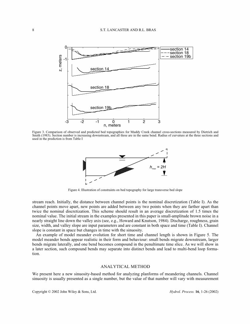
We used data from Muddy Creek, Wyoming (Dietrich and Smith, 1983, 1984; Dietrich and Whiting,1989), for the model parameter set (Table I) and testing of the transverse bed slope model. The transversebed slope predicted by Equations (9) and (11) is compared to cross-sections measured by Dietrich and Smith(1983) in Figure 3. Ikeda’s (1989) unmodified formula, i.e., Equation (10), predicted a transverse bed slopeapproximately twice as large. We predict the same transverse bed slope for each of the three sectionsbecause the curvature is the same at each. In reality, the transverse bed slope seems to “lag” behind the pre-diction such that the predicted slopes are too large for the first two sections (see Zhou et al., 1993, for a pre-diction of this “phase lag”). Johannesson and Parker (1989c) used an effective curvature that integratedcontributions from upstream to account for this lag. Typically, this lag is quite small, and, for our simplemodel, such complication is probably unwarranted.
Our solution for the transverse bed slope is most accurate at the channel centerline and least accurate at thebanks, and this error is larger for larger transverse bed slopes. Ikeda (1989) solved for the bed topographyover the entire channel width and showed that the transverse bed slope is lower over the point bar and in thedeepest part of the pool, especially when grain size is allowed to vary laterally. For large transverse bedslopes we constrain the bed topography by “chopping off” any part of the bed that would rise above the freewater surface and, to keep the cross-sectional area constant, any part of the pool that would sink below twicethe average depth (Figure 4a). These constraints are arbitrary but effectively limit the error for large trans-verse bed slopes, i.e., .
When Equations (4), (9), and (10) are applied to an ideal, sine-generated channel centerline, the lateralforce increment’s maximum magnitude is similar to that of the bottom shear stress integrated over a channelincrement (Lancaster, 1998). This result is consistent with the findings of Dietrich and Smith (1983) andDietrich and Whiting (1989) that these two forces are of similar magnitude and indicates that our representa-tion of the lateral forcing is accurate to within an order of magnitude.
We use a finite difference method to solve for the lateral migration (Equation 8) at discrete points along a
K Ψ′Ψ------ Ψ′
Ψcr--------- 0.2278
κ---------------- 11.0Ψ′H
Ψd50----------------------
ln 0.3606–=
Ψ′
ST 2H b⁄>
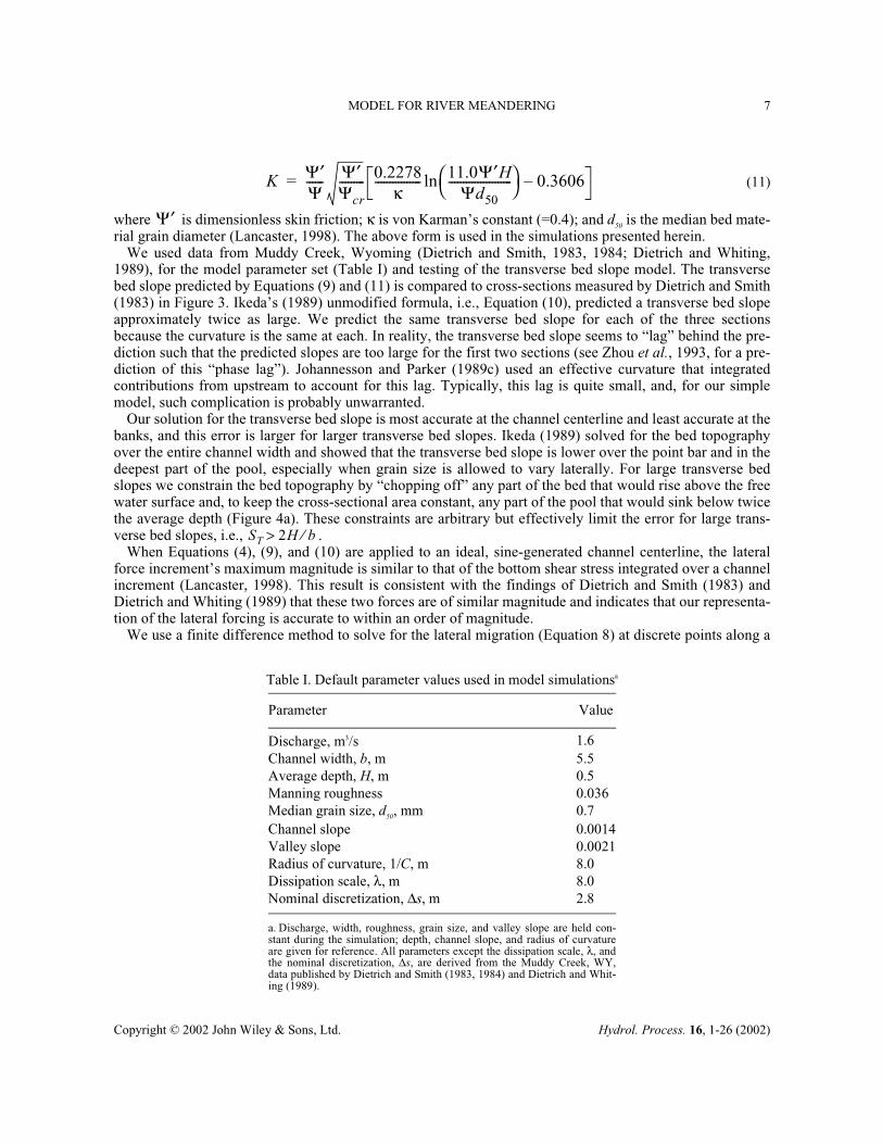
Table I. Default parameter values used in model simulationsa
a. Discharge, width, roughness, grain size, and valley slope are held con-stant during the simulation; depth, channel slope, and radius of curvatureare given for reference. All parameters except the dissipation scale, λ, andthe nominal discretization, ∆s, are derived from the Muddy Creek, WY,data published by Dietrich and Smith (1983, 1984) and Dietrich and Whit-ing (1989).
Parameter Value
Discharge, m3/s 1.6Channel width, b, m 5.5Average depth, H, m 0.5Manning roughness 0.036Median grain size, d50, mm 0.7Channel slope 0.0014Valley slope 0.0021Radius of curvature, 1/C, m 8.0Dissipation scale, λ, m 8.0Nominal discretization, ∆s, m 2.8
Copyright © 2002 John Wiley & Sons, Ltd. Hydrol. Process. 16, 1-26 (2002)
8 S.T. LANCASTER AND R.L. BRAS
stream reach. Initially, the distance between channel points is the nominal discretization (Table I). As thechannel points move apart, new points are added between any two points when they are farther apart thantwice the nominal discretization. This scheme should result in an average discretization of 1.5 times thenominal value. The initial stream in the examples presented in this paper is small-amplitude brown noise in anearly straight line down the valley axis (see, e.g., Howard and Knutson, 1984). Discharge, roughness, grainsize, width, and valley slope are input parameters and are constant in both space and time (Table I). Channelslope is constant in space but changes in time with the sinuosity.
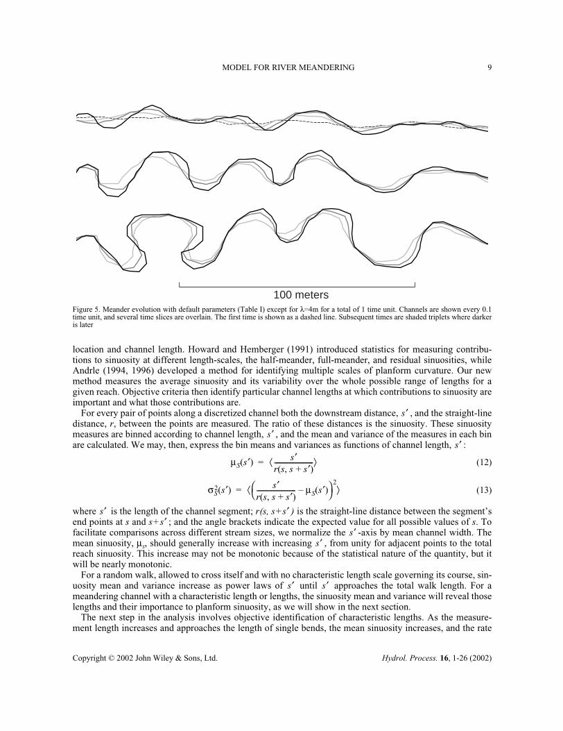
An example of model meander evolution for short time and channel length is shown in Figure 5. Themodel meander bends appear realistic in their form and behaviour: small bends migrate downstream, largerbends migrate laterally, and one bend becomes compound in the penultimate time slice. As we will show ina later section, such compound bends may separate into distinct bends and lead to multi-bend loop forma-tion.
ANALYTICAL METHOD
We present here a new sinuosity-based method for analyzing planforms of meandering channels. Channelsinuosity is usually presented as a single number, but the value of that number will vary with measurement
0
-1
-3 -2 -1 0 1 2 3
section 14
section 18
section 19b
n, meters
z, m
eter
s
section 14section 18section 19b
hmax = 2H
Figure 3. Comparison of observed and predicted bed topographies for Muddy Creek channel cross-sections measured by Dietrich andSmith (1983). Section number is increasing downstream, and all three are in the same bend. Radius of curvature at the three sections andused in the prediction is from Table I
Figure 4. Illustration of constraints on bed topography for large transverse bed slope
Copyright © 2002 John Wiley & Sons, Ltd. Hydrol. Process. 16, 1-26 (2002)
MODEL FOR RIVER MEANDERING 9
location and channel length. Howard and Hemberger (1991) introduced statistics for measuring contribu-tions to sinuosity at different length-scales, the half-meander, full-meander, and residual sinuosities, whileAndrle (1994, 1996) developed a method for identifying multiple scales of planform curvature. Our newmethod measures the average sinuosity and its variability over the whole possible range of lengths for agiven reach. Objective criteria then identify particular channel lengths at which contributions to sinuosity areimportant and what those contributions are.
For every pair of points along a discretized channel both the downstream distance, , and the straight-linedistance, r, between the points are measured. The ratio of these distances is the sinuosity. These sinuositymeasures are binned according to channel length, , and the mean and variance of the measures in each binare calculated. We may, then, express the bin means and variances as functions of channel length, :
(12)
(13)
where is the length of the channel segment; r(s, s+ ) is the straight-line distance between the segment’send points at s and s+ ; and the angle brackets indicate the expected value for all possible values of s. Tofacilitate comparisons across different stream sizes, we normalize the -axis by mean channel width. Themean sinuosity, µS, should generally increase with increasing , from unity for adjacent points to the totalreach sinuosity. This increase may not be monotonic because of the statistical nature of the quantity, but itwill be nearly monotonic.
For a random walk, allowed to cross itself and with no characteristic length scale governing its course, sin-uosity mean and variance increase as power laws of until approaches the total walk length. For ameandering channel with a characteristic length or lengths, the sinuosity mean and variance will reveal thoselengths and their importance to planform sinuosity, as we will show in the next section.
The next step in the analysis involves objective identification of characteristic lengths. As the measure-ment length increases and approaches the length of single bends, the mean sinuosity increases, and the rate
s′
s′s′
µS s′( ) s′r s s s′+,( )------------------------⟨ ⟩=
σS2 s′( ) s′
r s s s′+,( )------------------------ µS s′( )–
2⟨ ⟩=
s′ s′s′
s′s′
s′ s′
100 metersFigure 5. Meander evolution with default parameters (Table I) except for λ=4m for a total of 1 time unit. Channels are shown every 0.1time unit, and several time slices are overlain. The first time is shown as a dashed line. Subsequent times are shaded triplets where darkeris later
Copyright © 2002 John Wiley & Sons, Ltd. Hydrol. Process. 16, 1-26 (2002)
10 S.T. LANCASTER AND R.L. BRAS
of its increase also increases because typical channel segments tend to curve back on themselves as measure-ment length increases. As measurement lengths surpass the typical bend length, mean sinuosity may con-tinue to increase, but the rate decreases because at least some channel segments stop curving back onthemselves. The length of simple bends, , will be identified by that decrease in slope. At greater lengthsmany measurements will have moderate sinuosity and encompass more than one bend, but some measure-ments will encompass longer, particularly sinuous bends and loops that will weight the mean toward largervalues and make the sinuosity variance large. At such lengths there will be peaks in σS
2( ) and, possibly,corresponding inflections in µS( ). The first such peak in σS
2( ) will identify the length, . This lengthwill likely be that of particularly long simple or compound bends. If the first peak in σS
2( ) is not the larg-est, then the largest peak in σS
2( ) will identify a length we will call . Otherwise will be identified bythe next-largest peak in σS
2( ). This last length, , will likely correspond to multi-bend loops that makeimportant contributions to total sinuosity. The lengths defined above represent a simple and objective set ofcriteria for determining characteristic length-scales. Plots of mean sinuosity at each length versus the lengthsthemselves will facilitate comparison among planforms and detection of similar, or dissimilar, features. Inorder to determine what the above lengths represent, we will find examples of planform features, such asindividual bends, that have the same length as the identified length-scales.
ANALYSIS OF NATURAL CHANNELS
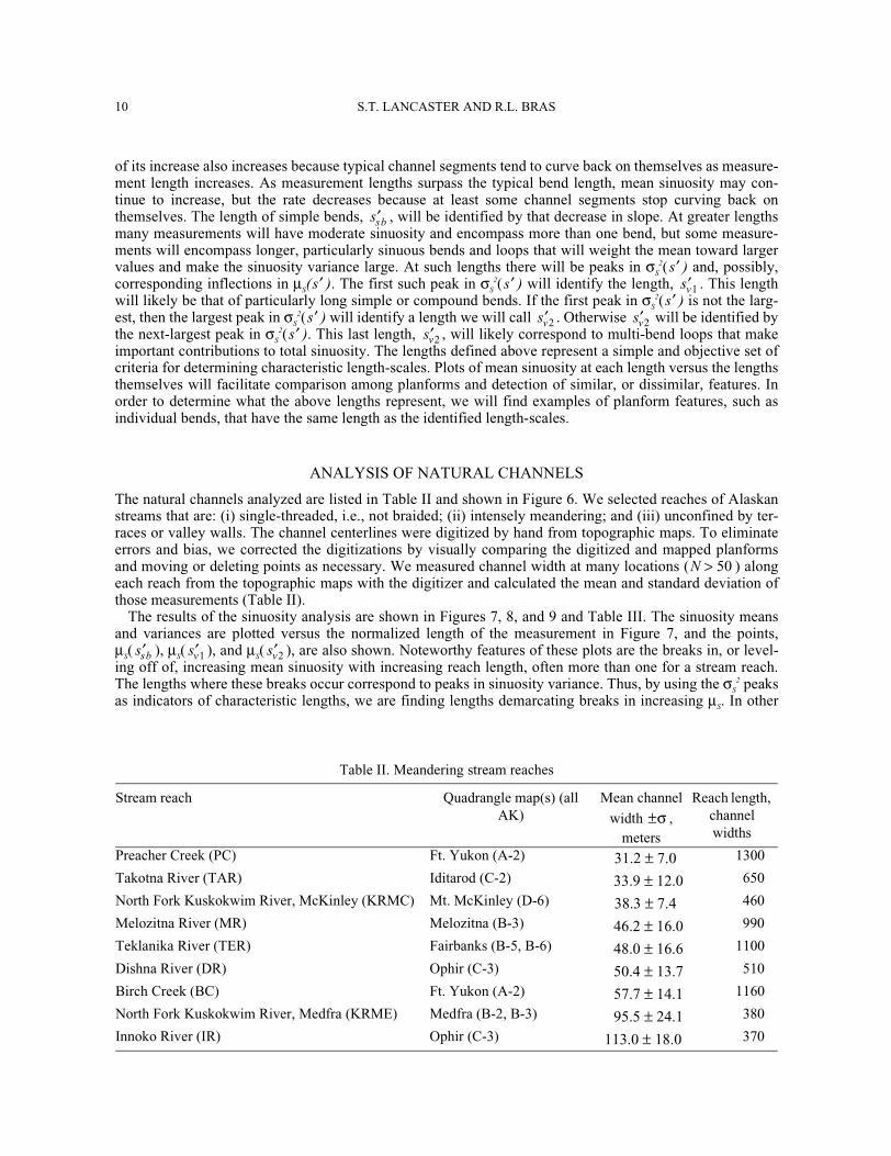
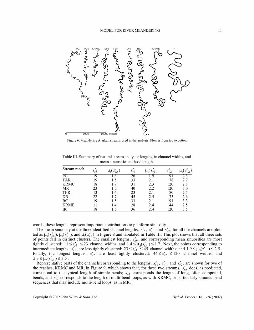
The natural channels analyzed are listed in Table II and shown in Figure 6. We selected reaches of Alaskanstreams that are: (i) single-threaded, i.e., not braided; (ii) intensely meandering; and (iii) unconfined by ter-races or valley walls. The channel centerlines were digitized by hand from topographic maps. To eliminateerrors and bias, we corrected the digitizations by visually comparing the digitized and mapped planformsand moving or deleting points as necessary. We measured channel width at many locations ( ) alongeach reach from the topographic maps with the digitizer and calculated the mean and standard deviation ofthose measurements (Table II).
The results of the sinuosity analysis are shown in Figures 7, 8, and 9 and Table III. The sinuosity meansand variances are plotted versus the normalized length of the measurement in Figure 7, and the points,µS( ), µS( ), and µS( ), are also shown. Noteworthy features of these plots are the breaks in, or level-ing off of, increasing mean sinuosity with increasing reach length, often more than one for a stream reach.The lengths where these breaks occur correspond to peaks in sinuosity variance. Thus, by using the σS
2 peaksas indicators of characteristic lengths, we are finding lengths demarcating breaks in increasing µS. In other
s′sb
s′s′ s′ s′v1
s′s′ s′v2 s′v2
s′ s′v2
N 50>
s′sb s′v1 s′v2
Table II. Meandering stream reaches
Stream reach Quadrangle map(s) (all AK)
Mean channel
width , meters
Reach length, channel widths
Preacher Creek (PC) Ft. Yukon (A-2) 1300
Takotna River (TAR) Iditarod (C-2) 650
North Fork Kuskokwim River, McKinley (KRMC) Mt. McKinley (D-6) 460
Melozitna River (MR) Melozitna (B-3) 990
Teklanika River (TER) Fairbanks (B-5, B-6) 1100
Dishna River (DR) Ophir (C-3) 510
Birch Creek (BC) Ft. Yukon (A-2) 1160
North Fork Kuskokwim River, Medfra (KRME) Medfra (B-2, B-3) 380
σ±
31.2 7.0±33.9 12.0±38.3 7.4±46.2 16.0±48.0 16.6±50.4 13.7±57.7 14.1±95.5 24.1±
Copyright © 2002 John Wiley & Sons, Ltd. Hydrol. Process. 16, 1-26 (2002)Innoko River (IR) Ophir (C-3) 370113.0 18.0±
MODEL FOR RIVER MEANDERING 11
words, these lengths represent important contributions to planform sinuosity. The mean sinuosity at the three identified channel lengths, , , and , for all the channels are plot-
ted as µS( ), µS( ), and µS( ) in Figure 8 and tabulated in Table III. This plot shows that all three setsof points fall in distinct clusters. The smallest lengths, , and corresponding mean sinuosities are mosttightly clustered: channel widths; and . Next, the points corresponding tointermediate lengths, , are less tightly clustered: channel widths; and .Finally, the longest lengths, , are least tightly clustered: channel widths; and
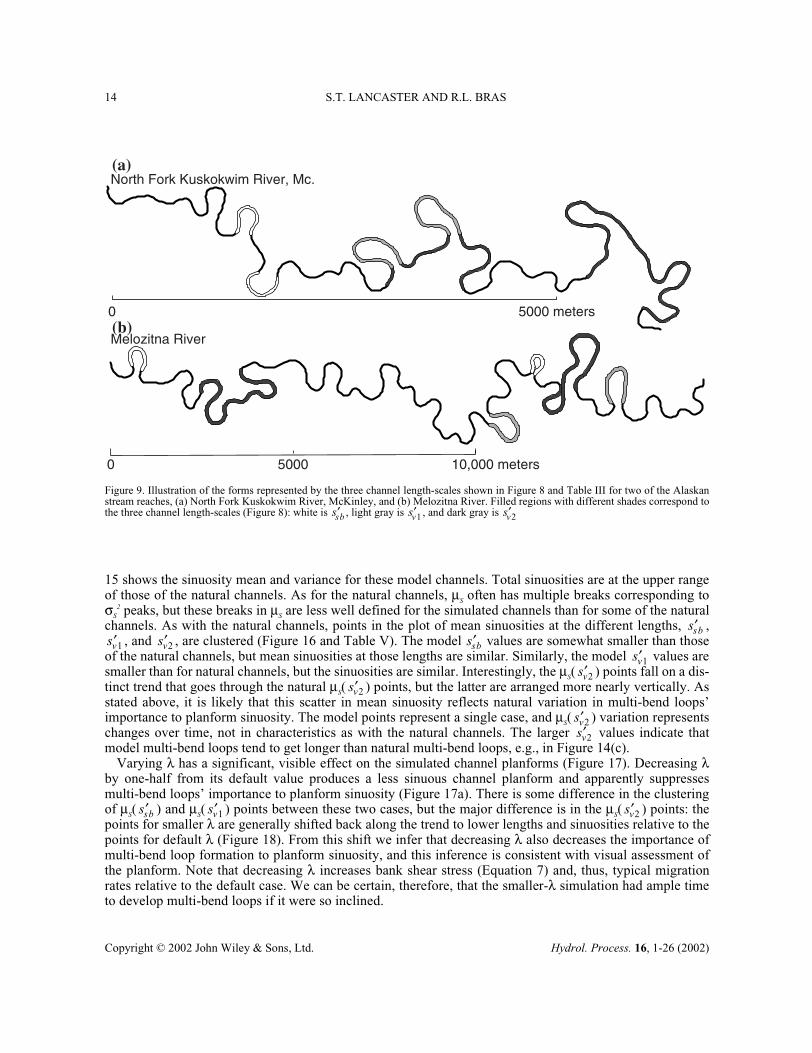
. Representative parts of the channels corresponding to the lengths, , , and , are shown for two of
the reaches, KRMC and MR, in Figure 9, which shows that, for these two streams, does, as predicted,correspond to the typical length of simple bends; corresponds the length of long, often compound,bends; and corresponds to the length of multi-bend loops, as with KRMC, or particularly sinuous bendsequences that may include multi-bend loops, as in MR.
s′sb s′v1 s′v2s′sb s′v1 s′v2
s′sb11 s′sb 23≤ ≤ 1.4 µS s′sb( ) 1.7≤ ≤
s′v1 23 s′v1 45≤ ≤ 1.9 µS s′v1( ) 2.5≤ ≤s′v2 44 s′v2 120≤ ≤
2.3 µS s′v2( ) 3.5≤ ≤s′sb s′v1 s′v2
s′sbs′v1
s′v2
PC KRMC DRTER BC KRMEMRTAR IR
0 5000 10000 meters
Figure 6. Meandering Alaskan streams used in the analysis. Flow is from top to bottom
Table III. Summary of natural stream analysis: lengths, in channel widths, and mean sinuosities at those lengths
Stream reach µS( ) µS( ) µS( )PC 19 1.6 26 1.9 91 2.3TAR 19 1.5 33 2.1 78 2.7KRMC 18 1.7 31 2.3 120 2.8MR 23 1.5 40 2.2 120 3.0TER 13 1.6 23 2.1 80 2.5DR 22 1.7 45 2.5 73 2.6BC 19 1.5 33 2.1 91 3.3KRME 11 1.4 28 2.4 44 2.5IR 18 1.5 36 2.4 120 3.5
s′sb s′sb s′v1 s′v1 s′v2 s′v2
Copyright © 2002 John Wiley & Sons, Ltd. Hydrol. Process. 16, 1-26 (2002)
12 S.T. LANCASTER AND R.L. BRAS
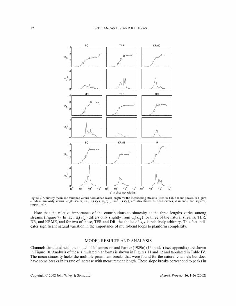
Note that the relative importance of the contributions to sinuosity at the three lengths varies amongstreams (Figure 7). In fact, µS( ) differs only slightly from µS( ) for three of the natural streams, TER,DR, and KRME, and for two of those, TER and DR, the choice of is relatively arbitrary. This fact indi-cates significant natural variation in the importance of multi-bend loops to planform complexity.
MODEL RESULTS AND ANALYSIS
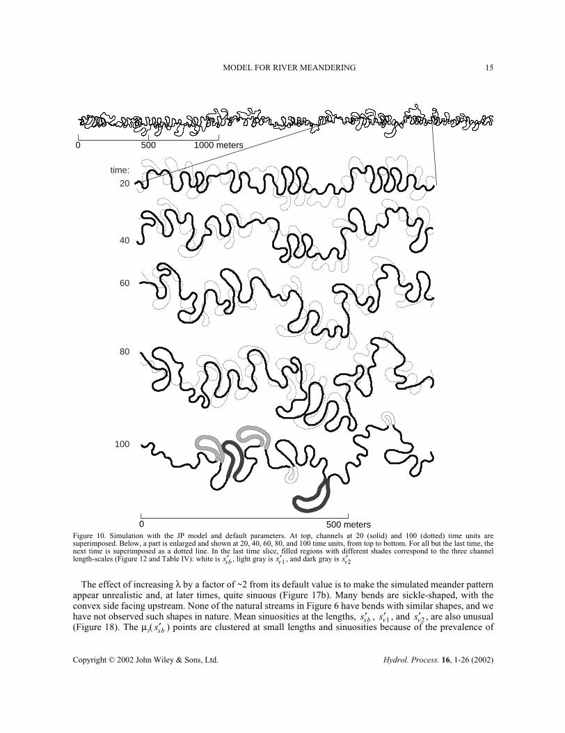
Channels simulated with the model of Johannesson and Parker (1989c) (JP model) (see appendix) are shownin Figure 10. Analysis of these simulated planforms is shown in Figures 11 and 12 and tabulated in Table IV.The mean sinuosity lacks the multiple prominent breaks that were found for the natural channels but doeshave some breaks in its rate of increase with measurement length. These slope breaks correspond to peaks in
s′v2 s′v1s′v2
1
2
3
4 PC
0
2
4
TAR KRMC
1
2
3
4 MR
0
2
4
TER DR
1
2
3
4 BC
100
101
102
103
0
2
4
KRME
100
101
102
103
IR
100
101
102
103
s' in channel widths
S
2S
S
2S
S
2S
Figure 7. Sinuosity mean and variance versus normalized reach length for the meandering streams listed in Table II and shown in Figure6. Mean sinuosity versus length-scales, i.e., µS( ), µS( ), and µS( ), are also shown as open circles, diamonds, and squares,respectively
s′sb s′v1 s′v2
Copyright © 2002 John Wiley & Sons, Ltd. Hydrol. Process. 16, 1-26 (2002)
MODEL FOR RIVER MEANDERING 13
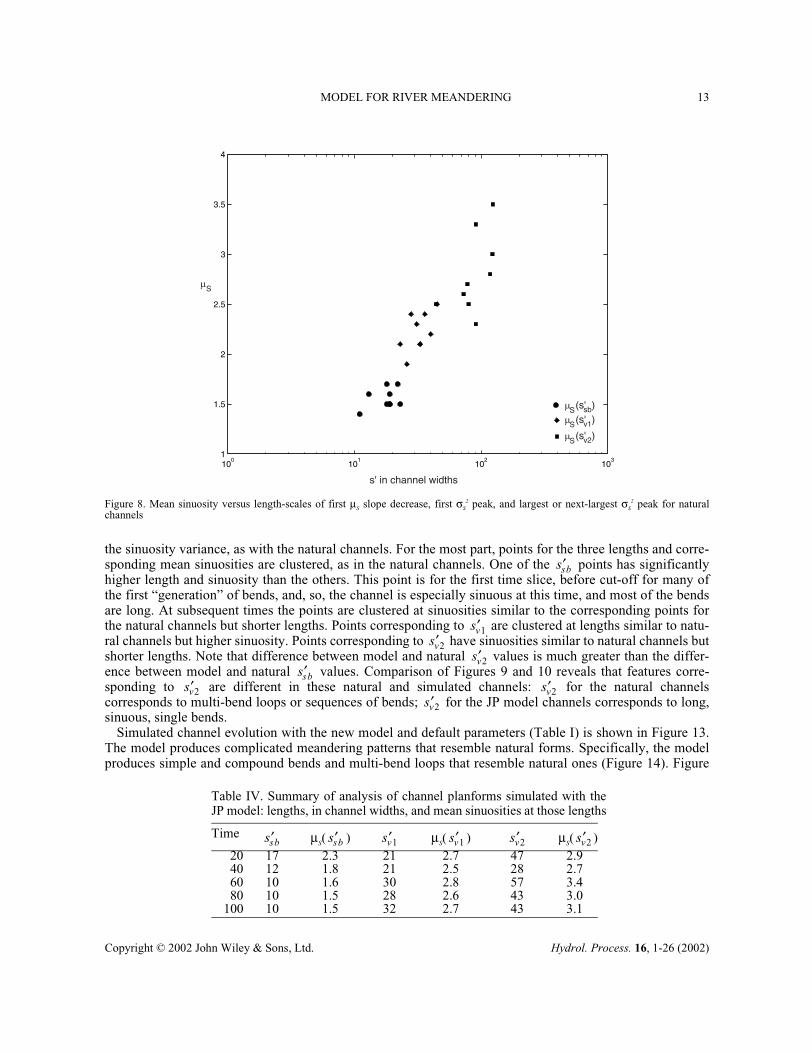
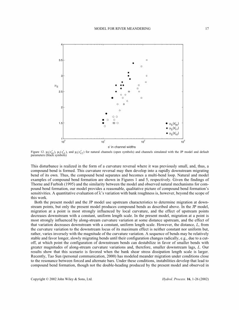
the sinuosity variance, as with the natural channels. For the most part, points for the three lengths and corre-sponding mean sinuosities are clustered, as in the natural channels. One of the points has significantlyhigher length and sinuosity than the others. This point is for the first time slice, before cut-off for many ofthe first “generation” of bends, and, so, the channel is especially sinuous at this time, and most of the bendsare long. At subsequent times the points are clustered at sinuosities similar to the corresponding points forthe natural channels but shorter lengths. Points corresponding to are clustered at lengths similar to natu-ral channels but higher sinuosity. Points corresponding to have sinuosities similar to natural channels butshorter lengths. Note that difference between model and natural values is much greater than the differ-ence between model and natural values. Comparison of Figures 9 and 10 reveals that features corre-sponding to are different in these natural and simulated channels: for the natural channelscorresponds to multi-bend loops or sequences of bends; for the JP model channels corresponds to long,sinuous, single bends.
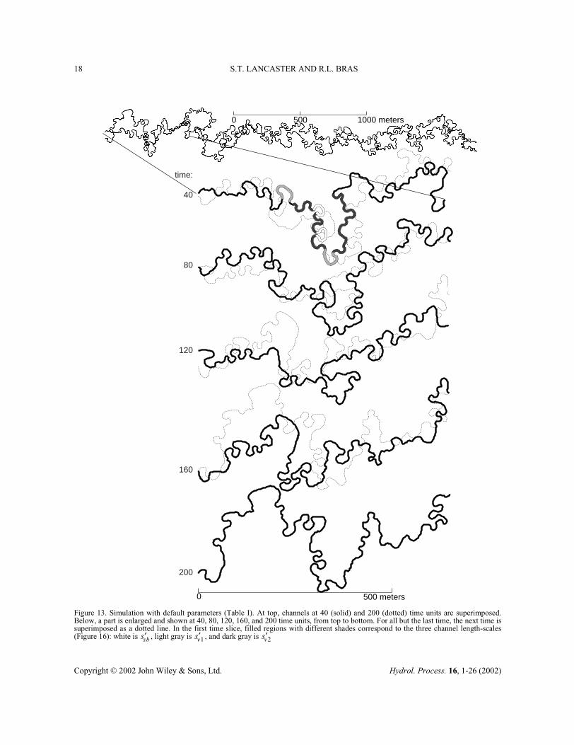
Simulated channel evolution with the new model and default parameters (Table I) is shown in Figure 13.The model produces complicated meandering patterns that resemble natural forms. Specifically, the modelproduces simple and compound bends and multi-bend loops that resemble natural ones (Figure 14). Figure
s′sb
s′v1s′v2
s′v2s′sb
s′v2 s′v2s′v2
100
101
102
103
1
1.5
2
2.5
3
3.5
4
S
s' in channel widths
(s' )S sb(s' )S v1
(s' )S v2
Figure 8. Mean sinuosity versus length-scales of first µS slope decrease, first σS2 peak, and largest or next-largest σS
2 peak for naturalchannels
Table IV. Summary of analysis of channel planforms simulated with theJP model: lengths, in channel widths, and mean sinuosities at those lengths
Time µS( ) µS( ) µS( )20 17 2.3 21 2.7 47 2.940 12 1.8 21 2.5 28 2.760 10 1.6 30 2.8 57 3.480 10 1.5 28 2.6 43 3.0
100 10 1.5 32 2.7 43 3.1
s′sb s′sb s′v1 s′v1 s′v2 s′v2
Copyright © 2002 John Wiley & Sons, Ltd. Hydrol. Process. 16, 1-26 (2002)
14 S.T. LANCASTER AND R.L. BRAS
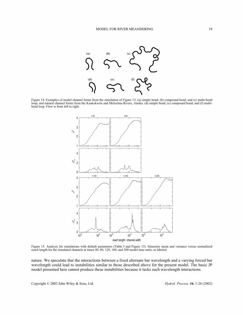
15 shows the sinuosity mean and variance for these model channels. Total sinuosities are at the upper rangeof those of the natural channels. As for the natural channels, µS often has multiple breaks corresponding toσS
2 peaks, but these breaks in µS are less well defined for the simulated channels than for some of the naturalchannels. As with the natural channels, points in the plot of mean sinuosities at the different lengths, ,
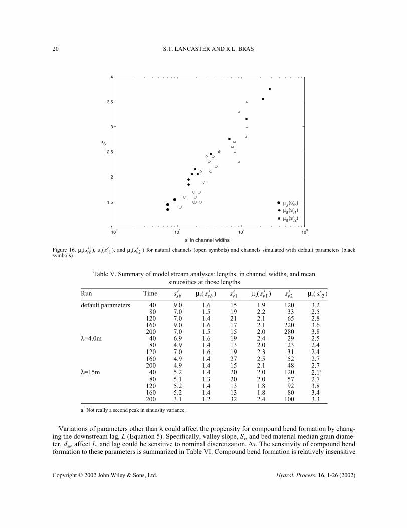
, and , are clustered (Figure 16 and Table V). The model values are somewhat smaller than thoseof the natural channels, but mean sinuosities at those lengths are similar. Similarly, the model values aresmaller than for natural channels, but the sinuosities are similar. Interestingly, the µS( ) points fall on a dis-tinct trend that goes through the natural µS( ) points, but the latter are arranged more nearly vertically. Asstated above, it is likely that this scatter in mean sinuosity reflects natural variation in multi-bend loops’importance to planform sinuosity. The model points represent a single case, and µS( ) variation representschanges over time, not in characteristics as with the natural channels. The larger values indicate thatmodel multi-bend loops tend to get longer than natural multi-bend loops, e.g., in Figure 14(c).
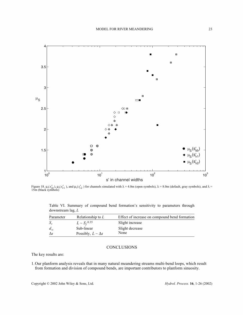
Varying λ has a significant, visible effect on the simulated channel planforms (Figure 17). Decreasing λby one-half from its default value produces a less sinuous channel planform and apparently suppressesmulti-bend loops’ importance to planform sinuosity (Figure 17a). There is some difference in the clusteringof µS( ) and µS( ) points between these two cases, but the major difference is in the µS( ) points: thepoints for smaller λ are generally shifted back along the trend to lower lengths and sinuosities relative to thepoints for default λ (Figure 18). From this shift we infer that decreasing λ also decreases the importance ofmulti-bend loop formation to planform sinuosity, and this inference is consistent with visual assessment ofthe planform. Note that decreasing λ increases bank shear stress (Equation 7) and, thus, typical migrationrates relative to the default case. We can be certain, therefore, that the smaller-λ simulation had ample timeto develop multi-bend loops if it were so inclined.
s′sbs′v1 s′v2 s′sb
s′v1s′v2
s′v2
s′v2s′v2
s′sb s′v1 s′v2
0 5000 10,000 meters
Melozitna River
North Fork Kuskokwim River, Mc.
0 5000 meters
(a)
(b)
Figure 9. Illustration of the forms represented by the three channel length-scales shown in Figure 8 and Table III for two of the Alaskanstream reaches, (a) North Fork Kuskokwim River, McKinley, and (b) Melozitna River. Filled regions with different shades correspond tothe three channel length-scales (Figure 8): white is , light gray is , and dark gray is s′sb s′v1 s′v2
Copyright © 2002 John Wiley & Sons, Ltd. Hydrol. Process. 16, 1-26 (2002)
MODEL FOR RIVER MEANDERING 15
The effect of increasing λ by a factor of ~2 from its default value is to make the simulated meander patternappear unrealistic and, at later times, quite sinuous (Figure 17b). Many bends are sickle-shaped, with theconvex side facing upstream. None of the natural streams in Figure 6 have bends with similar shapes, and wehave not observed such shapes in nature. Mean sinuosities at the lengths, , , and , are also unusual(Figure 18). The µS( ) points are clustered at small lengths and sinuosities because of the prevalence of
s′sb s′v1 s′v2s′sb
0 1000 meters500
0 500 meters
time:
20
40
60
80
100
Figure 10. Simulation with the JP model and default parameters. At top, channels at 20 (solid) and 100 (dotted) time units aresuperimposed. Below, a part is enlarged and shown at 20, 40, 60, 80, and 100 time units, from top to bottom. For all but the last time, thenext time is superimposed as a dotted line. In the last time slice, filled regions with different shades correspond to the three channellength-scales (Figure 12 and Table IV): white is , light gray is , and dark gray is s′sb s′v1 s′v2
Copyright © 2002 John Wiley & Sons, Ltd. Hydrol. Process. 16, 1-26 (2002)
16 S.T. LANCASTER AND R.L. BRAS
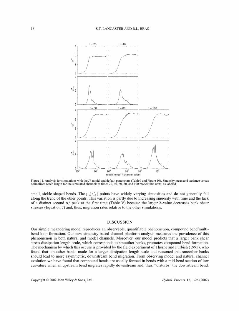
small, sickle-shaped bends. The µS( ) points have widely varying sinuosities and do not generally fallalong the trend of the other points. This variation is partly due to increasing sinuosity with time and the lackof a distinct second σS
2 peak at the first time (Table V) because the larger λ-value decreases bank shearstresses (Equation 7) and, thus, migration rates relative to the other simulations.
DISCUSSION
Our simple meandering model reproduces an observable, quantifiable phenomenon, compound bend/multi-bend loop formation. Our new sinuosity-based channel planform analysis measures the prevalence of thisphenomenon in both natural and model channels. Moreover, our model predicts that a larger bank shearstress dissipation length scale, which corresponds to smoother banks, promotes compound bend formation.The mechanism by which this occurs is provided by the field experiment of Thorne and Furbish (1995), whofound that smoother banks made for a larger dissipation length scale and reasoned that smoother banksshould lead to more asymmetric, downstream bend migration. From observing model and natural channelevolution we have found that compound bends are usually formed in bends with a mid-bend section of lowcurvature when an upstream bend migrates rapidly downstream and, thus, “disturbs” the downstream bend.
s′v2
t = 20 t = 40
t = 60 t = 80 t = 100
100 102 100 102 100 102
reach length / channel width
1
2
3
4
0
2
4
S
S2
1
2
3
4
0
2
4
S
S2
Figure 11. Analysis for simulations with the JP model and default parameters (Table I and Figure 10). Sinuosity mean and variance versusnormalized reach length for the simulated channels at times 20, 40, 60, 80, and 100 model time units, as labeled
Copyright © 2002 John Wiley & Sons, Ltd. Hydrol. Process. 16, 1-26 (2002)
MODEL FOR RIVER MEANDERING 17
This disturbance is realized in the form of a curvature reversal where it was previously small, and, thus, acompound bend is formed. This curvature reversal may then develop into a rapidly downstream migratingbend of its own. Thus, the compound bend separates and becomes a multi-bend loop. Natural and modelexamples of compound bend formation are shown in Figures 1 and 5, respectively. Given the findings ofThorne and Furbish (1995) and the similarity between the model and observed natural mechanisms for com-pound bend formation, our model provides a reasonable, qualitative picture of compound bend formation’ssensitivities. A quantitative evaluation of λ’s variation with bank roughness is, however, beyond the scope ofthis work.
Both the present model and the JP model use upstream characteristics to determine migration at down-stream points, but only the present model produces compound bends as described above. In the JP model,migration at a point is most strongly influenced by local curvature, and the effect of upstream pointsdecreases downstream with a constant, uniform length scale. In the present model, migration at a point ismost strongly influenced by along-stream curvature variation at some distance upstream, and the effect ofthat variation decreases downstream with a constant, uniform length scale. However, the distance, L, fromthe curvature variation to the downstream locus of its maximum effect is neither constant nor uniform but,rather, varies inversely with the magnitude of the curvature variation. A sequence of bends may be relativelystable and favor longer, slowly migrating bends until their configuration changes radically, e.g., due to a cut-off, at which point the configuration of downstream bends can destabilize in favor of smaller bends withgreater magnitudes of along-stream curvature variations and, therefore, smaller downstream lags, L. Ourresults show that this scenario is favored when the bank shear stress dissipation length scale is larger.Recently, Tao Sun (personal communication, 2000) has modeled meander migration under conditions closeto the resonance between forced and alternate bars. Under these conditions, instabilities develop that lead tocompound bend formation, though not the double-heading produced by the present model and observed in
100
101
102
103
1
1.5
2
2.5
3
3.5
4
S
s' in channel widths
(s' )S sb(s' )S v1
(s' )S v2
Figure 12. µS( ), µS( ), and µS( ) for natural channels (open symbols) and channels simulated with the JP model and defaultparameters (black symbols)
s′sb s′v1 s′v2
Copyright © 2002 John Wiley & Sons, Ltd. Hydrol. Process. 16, 1-26 (2002)
18 S.T. LANCASTER AND R.L. BRAS
Copyright © 2002 John Wiley & Sons, Ltd. Hydrol. Process. 16, 1-26 (2002)
0 500 1000 meters
0 500 meters
time:
40
80
120
160
200
Figure 13. Simulation with default parameters (Table I). At top, channels at 40 (solid) and 200 (dotted) time units are superimposed.Below, a part is enlarged and shown at 40, 80, 120, 160, and 200 time units, from top to bottom. For all but the last time, the next time issuperimposed as a dotted line. In the first time slice, filled regions with different shades correspond to the three channel length-scales(Figure 16): white is , light gray is , and dark gray is s′sb s′v1 s′v2
MODEL FOR RIVER MEANDERING 19
nature. We speculate that the interactions between a fixed alternate bar wavelength and a varying forced barwavelength could lead to instabilities similar to those described above for the present model. The basic JPmodel presented here cannot produce these instabilities because it lacks such wavelength interactions.
(a) (b) (c)
(d) (e) (f)
Figure 14. Examples of model channel forms from the simulation of Figure 13: (a) simple bend; (b) compound bend; and (c) multi-bendloop; and natural channel forms from the Kuskokwim and Melozitna Rivers, Alaska: (d) simple bend; (e) compound bend; and (f) multi-bend loop. Flow is from left to right.
1
2
3
4
0
2
4
S
S2
1
2
3
4
0
2
4
S
S2
reach length / channel width10 0 10 210 0 10 210 0 10 2
t=40 t=80
t=120 t=160 t=200
Figure 15. Analysis for simulations with default parameters (Table I and Figure 13). Sinuosity mean and variance versus normalizedreach length for the simulated channels at times 40, 80, 120, 160, and 200 model time units, as labeled.
Copyright © 2002 John Wiley & Sons, Ltd. Hydrol. Process. 16, 1-26 (2002)
20 S.T. LANCASTER AND R.L. BRAS
Variations of parameters other than λ could affect the propensity for compound bend formation by chang-ing the downstream lag, L (Equation 5). Specifically, valley slope, SV, and bed material median grain diame-ter, d50, affect L, and lag could be sensitive to nominal discretization, ∆s. The sensitivity of compound bendformation to these parameters is summarized in Table VI. Compound bend formation is relatively insensitive
100
101
102
103
1
1.5
2
2.5
3
3.5
4
S
s' in channel widths
(s' )S sb(s' )S v1
(s' )S v2
Figure 16. µS( ), µS( ), and µS( ) for natural channels (open symbols) and channels simulated with default parameters (blacksymbols)
s′sb s′v1 s′v2
Table V. Summary of model stream analyses: lengths, in channel widths, and mean sinuosities at those lengths
Run Time µS( ) µS( ) µS( )
default parameters 40 9.0 1.6 15 1.9 120 3.280 7.0 1.5 19 2.2 33 2.5
120 7.0 1.4 21 2.1 65 2.8160 9.0 1.6 17 2.1 220 3.6200 7.0 1.5 15 2.0 280 3.8
λ=4.0m 40 6.9 1.6 19 2.4 29 2.580 4.9 1.4 13 2.0 23 2.4
120 7.0 1.6 19 2.3 31 2.4160 4.9 1.4 27 2.5 52 2.7200 4.9 1.4 15 2.1 48 2.7
λ=15m 40 5.2 1.4 20 2.0 120 2.1a
a. Not really a second peak in sinuosity variance.
80 5.1 1.3 20 2.0 57 2.7120 5.2 1.4 13 1.8 92 3.8160 5.2 1.4 13 1.8 80 3.4200 3.1 1.2 32 2.4 100 3.3
s′sb s′sb s′v1 s′v1 s′v2 s′v2
Copyright © 2002 John Wiley & Sons, Ltd. Hydrol. Process. 16, 1-26 (2002)
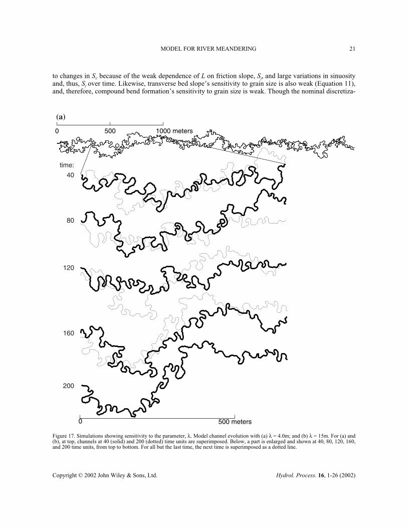
MODEL FOR RIVER MEANDERING 21
to changes in SV because of the weak dependence of L on friction slope, Sf, and large variations in sinuosityand, thus, Sf over time. Likewise, transverse bed slope’s sensitivity to grain size is also weak (Equation 11),and, therefore, compound bend formation’s sensitivity to grain size is weak. Though the nominal discretiza-
0 500 1000 meters
0 500 meters
time:
40
80
120
160
200
(a)
Figure 17. Simulations showing sensitivity to the parameter, λ. Model channel evolution with (a) λ = 4.0m; and (b) λ = 15m. For (a) and(b), at top, channels at 40 (solid) and 200 (dotted) time units are superimposed. Below, a part is enlarged and shown at 40, 80, 120, 160,and 200 time units, from top to bottom. For all but the last time, the next time is superimposed as a dotted line.
Copyright © 2002 John Wiley & Sons, Ltd. Hydrol. Process. 16, 1-26 (2002)

22 S.T. LANCASTER AND R.L. BRAS
tion could potentially affect the downstream lag, L, we found that finer discretization led to smaller bendsbut no change in compound bend formation. The discretization’s affect on the ‘texture’ of the simulatedform is not unusual to this model. In our own experience with landscape evolution models the horizontal dis-cretization of topography affects simulated landscape texture such that finer discretizations can lead tohigher drainage densities (Lancaster, 1998).
0 500 1000 meters
0 500 meters
time:
40
80
120
160
200
(b)
Figure 17. (Continued)
Copyright © 2002 John Wiley & Sons, Ltd. Hydrol. Process. 16, 1-26 (2002)
MODEL FOR RIVER MEANDERING 23
CONCLUSIONS
The key results are:
1.Our planform analysis reveals that in many natural meandering streams multi-bend loops, which result from formation and division of compound bends, are important contributors to planform sinuosity.
100
101
102
103
1
1.5
2
2.5
3
3.5
4
s' in channel widths
S
(s' )S sb(s' )S v1
(s' )S v2
Figure 18. µS( ), µS( ), and µS( ) for channels simulated with λ = 4.0m (open symbols), λ = 8.0m (default, gray symbols), and λ =15m (black symbols)
s′sb s′v1 s′v2
Table VI. Summary of compound bend formation’s sensitivity to parameters throughdownstream lag, L
Parameter Relationship to L Effect of increase on compound bend formationSV Slight increase
d50 Sub-linear Slight decrease∆s Possibly, None
L Sf0.35–∼
L s∆∼
Copyright © 2002 John Wiley & Sons, Ltd. Hydrol. Process. 16, 1-26 (2002)
24 S.T. LANCASTER AND R.L. BRAS
2.Previous, physics-based models, e.g., the JP model, do not accurately reproduce this contribution. 3.Our new model, with its simplified process representation, is sufficient to produce realistic meander evolu-
tion, during which compound bend and multi-bend loop formation emerge as primary mechanisms of planform evolution.
4.The model predicts that compound bend and multi-bend loop formation are sensitive to the interaction between two important lengths, the downstream lag between the bend entrance and the zone of maximum bank shear stress, L, and the distance over which that shear stress is dissipated, λ. Specifically, larger val-ues of λ, which correspond to smoother banks, lead to greater importance of multi-bend loop formation to planform sinuosity.
The implications for natural streams are that (i) multi-bend loops may result from primary process mecha-nisms rather than secondary phenomena, such as bank heterogeneity or alternate bars, and (ii) the prevalenceof multi-bend loop formation may be sensitive to bank roughness. Our analysis measures the prevalence ofmulti-bend loop formation, and bank roughness can be measured in the field or, perhaps, inferred from char-acteristics, such as bank vegetation, detectable with remote sensing. These implications, therefore, representa testable hypothesis motivating future work.
ACKNOWLEDGEMENTS
This research was supported by the U.S. Army Construction Engineering Research Laboratories (DACA 88-95-R-0020) while the first author was at the Massachusetts Institute of Technology. The views, opinions,and/or findings contained in this paper are those of the authors and should not be construed as an officialDepartment of the Army position, policy, or decision, unless so designated by other documentation. Thisresearch has also been supported by the CLAMS Project, Pacific Northwest Research Station of the USDAForest Service, since the first author moved to Oregon State University. We are grateful to Gordon Grant,Shannon Hayes, Gregory Tucker, and Kelin Whipple for discussion and thoughtful comments, Jim Pizzutofor a helpful review of an earlier version, and Rob Ferguson and an anonymous reviewer for helpful reviews.
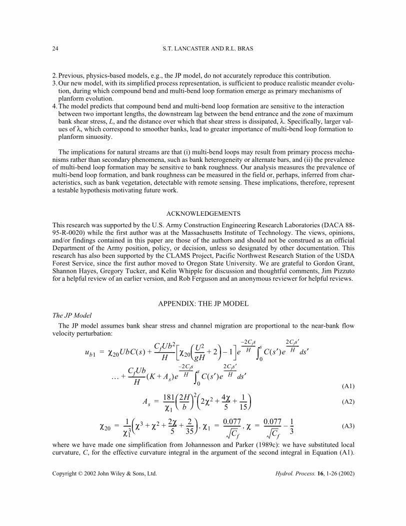
APPENDIX: THE JP MODEL
The JP Model
The JP model assumes bank shear stress and channel migration are proportional to the near-bank flowvelocity perturbation:
(A1)
(A2)
, , (A3)
where we have made one simplification from Johannesson and Parker (1989c): we have substituted localcurvature, C, for the effective curvature integral in the argument of the second integral in Equation (A1).
ub1 χ20UbC s( )CfUb2
H---------------- χ20
U2
gH------- 2+
1– e2Cfs–H
--------------C s′( )e
2Cfs′H
-------------s′d
0
s
∫+=
…CfUb
H-------------+ K As+( )e
2Cfs–H
--------------C s′( )e
2Cfs′H
-------------s′d
0
s
∫
As181χ1
--------- 2Hb
------- 2
2χ2 4χ5
------ 115------+ +
=
χ201
χ13
------ χ3 χ2 2χ5
------ 235------+ + +
= χ10.077
Cf
-------------= χ 0.077
Cf
------------- 13---–=
Copyright © 2002 John Wiley & Sons, Ltd. Hydrol. Process. 16, 1-26 (2002)
MODEL FOR RIVER MEANDERING 25
This substitution makes the JP model more directly comparable to ours, and A.D. Howard (personal commu-nication, 1996) reports that the use of effective curvature rather than local curvature has an insignificanteffect on model behaviour.
REFERENCES
Andrle R. 1994. The angle measure technique: A new method for characterizing the complexity of geomorphic lines. Mathematical Geol-ogy 26: 83-97.
Andrle R. 1996. Measuring channel planform of meandering rivers. Physical Geography 17(3): 270-281. Beck S. 1984. Mathematical modeling of meander interaction. In River Meandering, Proceedings of the Conference, Rivers ‘83, Elliott
CM (ed). ASCE: New York; 932-941.Blondeaux P, Seminara G. 1985. A unified bar-bend theory of river meanders. Journal of Fluid Mechanics 157: 449-470.Brice J. 1974. Meandering pattern of the White River in Indiana--an analysis. In Fluvial Geomorphology, Morisawa M (ed). State Univer-
sity of New York: Binghamton; 178-200. Dietrich WE, Smith JD. 1983. Influence of the point bar on flow through curved channels. Water Resources Research 19(5): 1173-1192. Dietrich WE, Smith JD. 1984. Bed load transport in a river meander. Water Resources Research 20(10): 1355-1380.Dietrich WE, Whiting P. 1989. Boundary shear stress and sediment transport in river meanders of sand and gravel. In River Meandering,
Ikeda S, Parker G (eds). American Geophysical Union: Washington; 1-50.Engelund F, Hansen F. 1967. A monograph on sediment transport in alluvial streams. In Teknisk Verlag. Technical University of Den-
mark: Copenhagen; 63.Ferguson RI. 1984. Kinematic model of meander migration. In River Meandering, Proceedings of the Conference, Rivers ‘83, Elliott CM
(ed). ASCE: New York; 942-951. Furbish DJ. 1988. River-bend curvature and migration: How are they related? Geology 16: 752-755. Furbish DJ. 1991. Spatial autoregressive structure in meander evolution. GSA Bulletin 103(12): 1576-1589.Hasegawa K. 1989. Studies on qualitative and quantitative prediction of meander channel shift. In River Meandering, Ikeda S, Parker G
(eds). American Geophysical Union: Washington; 215-235.Hooke JM, Harvey AM. 1983. Meander changes in relation to bend morphology and secondary flows. Modern and Ancient Fluvial Sys-
tems, Collinson JD, Lewin J (eds). Special Publication of the International Association of Sedimentologists 6: 121-132.Howard AD. 1992. Modelling channel migration and floodplain development in meandering streams. In Lowland Floodplain Rivers, Car-
ling PA, Petts GE (eds). John Wiley & Sons: Chichester; 1-42.Howard AD. 1994. A detachment-limited model of drainage basin evolution. Water Resources Research 30(7): 2261-2285.Howard AD, Hemberger AT. 1991. Multivariate characterization of meandering. Geomorphology 4: 161-186.Howard AD, Knutson TR. 1984. Sufficient conditions for river meandering: A simulation approach. Water Resources Research 20(11):
1659-1667.Ikeda S. 1989. Sediment transport and sorting at bends. In River Meandering, Ikeda S, Parker G (eds). American Geophysical Union:
Washington; 103-126.Ikeda S, Parker G, Sawai K. 1981. Bend theory of river meanders. Part 1. Linear development. Journal of Fluid Mechanics 112: 363-377.Ikeda S, Yamasaka M, Chiyoda M. 1987. Bed topography and sorting in bends. Journal of Hydraulic Engineering 113(2): 190-206. Imran J, Parker G, Pirmez C. 1999. A nonlinear model of flow in meandering submarine and subaerial channels. Journal of Fluid
Mechanics 400: 295-331.Johannesson H, Parker G. 1985. Computer simulated migration of meandering rivers in Minnesota. Project Report No. 242. St. Anthony
Falls Hydraulic Laboratory: Minneapolis; 82. Johannesson H, Parker G. 1989a. Linear theory of river meanders. In River Meandering, Ikeda S, Parker G (eds). American Geophysical
Union: Washington; 181-214.Johannesson H, Parker G. 1989b. Secondary flow in mildly sinuous channel. Journal of Hydraulic Engineering 115(3): 289-308. Johannesson H, Parker G. 1989c. Velocity redistribution in meandering rivers. Journal of Hydraulic Engineering 115(8): 1019-1039. Lancaster ST. 1998. A Nonlinear River Meandering Model and its Incorporation in a Landscape Evolution Model. Ph.D. Thesis, Dept. of
Civil and Environmental Engineering, Massachusetts Institute of Technology: Cambridge; 277. Murray AB, Paola C. 1994. A cellular model of braided rivers. Nature 371(6492): 54-57.Murray AB, Paola C. 1997. Properties of a cellular braided-stream model. Earth Surface Processes and Landforms 22: 1001-1025.Nanson GC, Hickin EJ. 1983. Channel migration and incision on the Beatton River. Journal of Hydraulic Engineering 109: 327-337.Nelson JM, Smith JD. 1989a. Flow in meandering channels with natural topography. In River Meandering, Ikeda S, Parker G (eds).
American Geophysical Union: Washington; 69-102. Nelson JM, Smith JD. 1989b. Evolution and stability of erodible channel beds. In River Meandering, Ikeda S, Parker G (eds). American
Geophysical Union: Washington; 321-378.Odgaard AJ. 1982. Bed characteristics in alluvial channel bends. Journal of the Hydraulics Division 108(HY11): 1268-1281.Odgaard AJ. 1986. Meander flow model. I: Development. Journal of Hydraulic Engineering 112(12): 1117-1136. Paola C, Hellert PL, Angevine CL. 1992. The large-scale dynamics of grain-size variation in alluvial basins, 1: Theory. Basin Research 4:
73-90.Parker G, Sawai K, Ikeda S. 1982. Bend theory of river meanders. Part 2. Nonlinear deformation of finite-amplitude bends. Journal of
Fluid Mechanics 115: 303-314.
Copyright © 2002 John Wiley & Sons, Ltd. Hydrol. Process. 16, 1-26 (2002)
26 S.T. LANCASTER AND R.L. BRAS
Pizzuto JE, Meckelnburg TS. 1989. Evaluation of a linear bank erosion equation. Water Resources Research 25: 1005-1013. Seminara G, Tubino M. 1989. Alternate bars and meandering: Free, forced and mixed interactions. In River Meandering, Ikeda S, Parker
G (eds). American Geophysical Union: Washington; 267-320. Seminara G, Tubino M. 1992. Weakly nonlinear theory of regular meanders. Journal of Fluid Mechanics 244: 257-288. Smith JD, McLean SR. 1984. A model for flow in meandering streams. Water Resources Research 20(9): 1301-1315. Sun T, Meakin P, Jøssang T, Schwarz K. 1996. A simulation model for meandering rivers. Water Resources Research 32(9): 2937-2954. Thompson A. 1986. Secondary flows and the pool-riffle unit, a case study of the processes of meander development. Earth Surface Pro-
cesses and Landforms 11(6): 631-641.Thorne CR, Osman AM. 1988. Riverbank stability analysis, II, applications. Journal of Hydraulic Engineering 114(2): 151-172.Thorne SD, Furbish DJ. 1995. Influences of coarse bank roughness on flow within a sharply curved river bend. In Predicting Process
from Form, Whiting PJ, Furbish DJ (eds). Geomorphology 12(3): 241-257.Tucker GE, Slingerland RL. 1994. Erosional dynamics, flexural isostasy, and long-lived escarpments: a numerical modeling study. Jour-
nal of Geophysical Research 99: 12,229-12,243.Willgoose G, Bras RL, Rodriguez-Iturbe I. 1991. A physically based coupled network growth and hillslope evolution model, 1, theory.
Water Resources Research 27: 1671-1684.Zhou J, Chang H-H, Stow D. 1993. A model for phase lag of secondary flow in river meanders. Journal of Hydrology 146(1-4): 73-88.
Copyright © 2002 John Wiley & Sons, Ltd. Hydrol. Process. 16, 1-26 (2002)