Embed Size (px)
Citation preview

Hydraulic Fracturing: Past, Present, and Future An analysis of the economic and environmental impacts of “fracking” in the United States Group 9: Garrett Apel, Jamison Huang, Miguel Lora, Katie Oliver, Ivy Zhang

2
Acknowledgements We would like to thank the following people: Dr. R. Stephen Berry Dr. George Tolley Jaeyoon Lee Jing Wu

3
Table of Contents Acknowledgements ................................................................................................................................................. 2
Table of Contents ...................................................................................................................................................... 3 Abstract ........................................................................................................................................................................ 4
Timeline: Natural Gas Fracking in the U.S. .................................................................................................... 6
Overview and Motivation ..................................................................................................................................... 7 Techniques ............................................................................................................................................................................... 7 Natural Gas Fracking in the U.S. ..................................................................................................................................... 9 Major Shale Gas Plays ...................................................................................................................................................... 13 Uses of Natural Gas ........................................................................................................................................................... 15 Projections ............................................................................................................................................................................ 17
Competitive Landscape ....................................................................................................................................... 19
Timeline: Fracking Policies ............................................................................................................................... 25 Understanding Current Fracking Policies .................................................................................................. 26
Economic Benefits ................................................................................................................................................. 28 Haynesville Shale Analysis ................................................................................................................................ 32 Input Factors ........................................................................................................................................................................ 32 Expanding on the Input Factors .................................................................................................................................. 36 Operating Costs and Escalation .............................................................................................................................. 36 Approximating Natural Gas Prices ........................................................................................................................ 37
Gas Price/Escalation ......................................................................................................................................................... 38 Modeling Well Production Curve ................................................................................................................................ 39 Estimating Annual Decline of Well Production ..................................................................................................... 41 1) The percent annual decline forecast .............................................................................................................. 41 2) Decline curve model .............................................................................................................................................. 41
Evaluating Profitability ................................................................................................................................................... 42 Aggregate Economic Model ............................................................................................................................... 44 Results .................................................................................................................................................................................... 44 Gas production .................................................................................................................................................................... 47 Sensitivity Analysis ........................................................................................................................................................... 52
Environmental Repercussions of Hydraulic Fracturing ....................................................................... 54 Greenhouse gasses ............................................................................................................................................................ 55 Water use .............................................................................................................................................................................. 56 Water contamination ....................................................................................................................................................... 57 Costs of Environmental Factors .................................................................................................................................. 60
Policy Proposal ....................................................................................................................................................... 63 Conclusion and Further Discussion ............................................................................................................... 64
Works Referenced ................................................................................................................................................. 66

4
Abstract The use of hydraulic fracturing for hydrocarbon extraction has soared over the past decade. New
techniques pioneered in the United States have enabled extractors to target the vast reserves of
natural gas trapped in America’s shale formations. While the changes have revolutionized the
world’s energy landscape, they have been accompanied by controversy. Critics question the
safety record of this new technology and have raised concerns regarding negative environmental
externalities associated with fracking operations. This heated debate is occurring against a
backdrop of discussions involving climate change, economic growth and energy security. As
with many emerging technologies, government regulation trails implementation. Lawmakers
have struggled to keep up with the rapid technological developments in fracking and have faced
many challenges in attempting to analyze the benefits and costs of implementing this new
extraction method.
This report will attempt to devise an economically viable regulatory framework for dry natural
gas hydraulic fracturing operations. To do this, the report will cover five sections. The first
segment will involve a discussion of hydraulic fracturing as a whole, including details
surrounding technologies, production methods and the competitive landscape. The second
section will analyze, from a policy standpoint, the broad economic and strategic benefits of
utilizing hydraulic fracturing while also considering current policies surrounding the practice.
The third section will involve a complex model created to analyze the profitability of hydraulic
fracturing in the relative absence of environmental regulation. The fourth section of the report
will involve a qualitative analysis of the environmental costs accompanying hydraulic fracturing

5
and a quantitative analysis of the costs of mitigating those concerns. The report will conclude
with a policy recommendation based off of the quantitative analysis conducted earlier in the
report.

6
Timeline: Natural Gas Fracking in the U.S. 1860’s First use of liquid to stimulate shallow, hard rock wells in Pennsylvania, New York,
Kentucky and West Virginia. 1930’s Oil companies attempt to inject fluid into the ground to stimulate wells. The liquids
often included acid that created etchings along the fractures, allowing more oil and gas to escape.
1947 Stanolind Oil and Gas Corporation conducts the first true hydraulic fracturing
experiment, injecting 1,000 gallons of gelled gasoline and sand into the Hugoton gas field. The treatment did not significantly increase output.
1949 The Halliburton Oil Well Cementing Company patents emerging fracking
technology and conducts the first commercial hydraulic fractures in Stephens County, Oklahoma and Archer County, Texas.
1960’s The U.S. government explores “massive hydraulic fracturing,” using underground
nuclear explosions to fracture rock formations. The results are disappointing. 1965 First instance of hydraulic fracturing in shale formations. The treatments are minor,
but generally successful at increasing production. 1976 The Department of Energy initiates the Eastern Gas Shales Project, designed to
advance hydraulic fracturing techniques in shale formations and develop extraction methods for unconventional natural gas reserves.
1987 Union Pacific Resources enters the Austin Chalk play, revitalizing production with
horizontal well drilling and multistage massive slickwater hydraulic fracture treatments.
1997 Mitchell Energy develops present-day hydraulic fracturing methods, improving
treatments and adapting them for shale formations. They apply their new high-pressure method to the Barnett Shale.
2005+ Shale gas fracking booms, bringing both economic development and environmental
concerns.

7
Overview and Motivation
Techniques
Hydraulic fracturing, or fracking, utilizes new extraction technology to remove hydrocarbons
from geological formations. Fracking is used on formations with low permeability in an attempt
to increase the flow rate of the stored hydrocarbons, allowing them to move up the well for
extraction. Due to the typical geological conditions surrounding the hydrocarbon formations
targeted by fracking, the type of oil recovered is referred to as “tight oil”. Most of the growth and
controversy surrounding new natural gas production comes from fracking in shale formations,
and the product of this operation is simply called shale gas. The process, neglecting some

8
considerations which will be discussed momentarily, is shown in the image before (Granberg
2015). The hydrocarbons extracted as a result of this process vary considerably. They include
crude oil, dry gas (mostly methane—CH4) and wet gas (methane, along with other natural gas
liquids such as ethane and butane). Due to poor industry categorization of the different
hydrocarbons and the inaccuracies of data surrounding certain categories, this report will focus
on the considerations involving dry natural gas.
Fracking is the overwhelmingly preferred method of natural gas extraction, used in nine out of
ten natural gas wells in the U.S. The precise methods of fracking that are used vary from location
to location and depend on a variety of factors including the depth of the gas-rich shale layer, the
type of drilling technology used, and the availability of water. The depth at which fracking
occurs remains dependent on the geology of the region, which can present considerable
challenges—in many formations, companies have been known to extract natural gas at depths
exceeding 10,000 feet. While these depths may vary considerably, nearly all shale gas extraction
operations in the United States occur at depths far below the water table.
The drilling methods used in fracking have advanced significantly over the past few years. Some
techniques place wells horizontally within the shale layers, allowing fissures to develop over a
greater area. Newer technologies have enabled drillers to connect several horizontal wells to one
vertical well, allowing for more efficient gas extraction. Despite the various and rapid
technological advancements, the core processes surrounding natural gas extraction through
fracking have remained the same.

9
Natural Gas Fracking in the U.S.
Source: EIA 2012
Fracking has grown rapidly in the United States and now accounts for 43% of the oil production
and over two-thirds of the natural gas production in the country (Perry 2013). Much of the
growth in fracking usage has occurred in the past decade and has been spurred by technological
developments that occurred in the United States. As a result of this revolution in fracking
technology over the past decade, the production capabilities of the United States have increased
dramatically, far surpassing the previous production peak which occurred in 1973.
The recent sharp rise in production capabilities began in 2005. U.S. dry natural gas production
for that year totaled 18,050,598 million cubic feet. By 2014, dry natural gas production reached
25,728,498 million cubic feet, representing a 42.5% increase in production. This increase in

10
production has been accompanied by a surge in the number of unconventional natural gas wells,
whose numbers increased nearly 45% in the three year period from 2004 to 2007 (Solomon
2015).
The opening up of this new resource has also allowed for more exploration and higher estimates
of recoverable reserves. The Potential Gas Committee’s (PGC) 2015 report estimated that there
are 2,515 trillion cubic feet of natural gas in the U.S. that can be extracted given current
technologies. Current forecast production trends predict the natural gas supply to grow 1.8%
from 78.72 Bcf today to 80.52 Bcf per day in 2016. This estimate represents the highest
assessment in PCG’s 50 year history (PGC 2015), and continues the trend of increasing
projections. These estimates far surpass those made even a few years earlier; in 2006, PCG put
estimated natural gas reserves at 1,532 trillion cubic feet (PGC 2006).
As a result of the large increases in natural gas production through fracking, the U.S. has become
much less reliant on other nations’ reserves. While this newfound independence may be more
geopolitically important with regards to oil production, the natural gas boom has still
significantly altered the energy landscape. The growth of internal production has lowered
domestic natural gas prices, giving U.S.-produced natural gas a competitive advantage over
foreign-produced gas. Historically, the U.S. has imported a significant proportion of its gas.
However, in 2013, these imports were around 1.5 trillion cubic feet, representing the lowest
levels since 1989. In 2014, net imports fell an additional 9%. Exports, meanwhile, have more
than doubled since 2005 (EIA 2014).

11
As increases in domestic production increase energy independence and reduce demand for
natural gas imports, the United States will likely continue to increase exports, specifically to
Mexico. In August 2015, natural gas imports fell to a twenty-year low of 2.2 Bcf/day. The EIA
predicts an increase in exports to Mexico as a result of growing demand in their power sector as
well as flat production. A new liquefaction plant, Cheniere’s Sabine Pass LNG, will increase
exports to an average of 0.7 Bcf/day beginning in 2016 (EIA 2015).
The majority of this growth has been fueled by shale gas fracking. The figure below
demonstrates this, outlining the various sources of natural gas production in the U.S. In the
period 2009-2014, nearly all the sources of dry natural gas production stayed constant or showed
a slight decrease. However, production from shale gas wells increased dramatically, going from
3,958,315 million cubic feet in 2009 to 11,896,204 million cubic feet in 2014. This roughly
represents a tripling in the production of shale natural gas (EIA 2014).

12
The development of new fracking techniques has been largely centered in the United States. As a
result, the U.S. has developed a competitive advantage in production capabilities. Production has
soared relative to other countries, and in 2014 the U.S. was the world’s largest producer of
natural gas (CIA 2015).
U.S. natural gas production surpassed that of Russia between 2009 and 2010. The production
from both of these countries, however, dwarfs that of the next four highest producing states.
While this recent lead remains as of 2015, the spread of fracking technology, accompanied by an
increase in global shale gas exploration, is expected to blunt the U.S.’s production advantage
relative to other countries.

13
Major Shale Gas Plays Fracking operations in the United States are not evenly distributed across the country. Rather,
they occur in discrete geological formations interspersed throughout the nation, as shown below
(EIA 2010).
Each geological formation has a unique deformation history associated with it. The type and
scale of naturally occurring hydrocarbons in a given formation is determined by several factors.
These include the organic matter content of the sediment and the magnitude of compression and
heating. Additional formation-specific information can be gleaned from basin modelling and
improved petrophysical characterizations. Though all the formations have dry natural gas, wet
natural gas and oil, the ratios of these hydrocarbons differs from field to field. While this report

14
will focus on the plays with the highest dry natural gas content, it should be noted that some less-
discussed formations (such as the Bakken) are critical to U.S. energy production due to their high
oil output.
The three largest shale gas plays in the U.S. are in the Marcellus, Haynesville and Barnett shales.
All three of these plays occur in basins. The Marcellus shale is located in the Appalachian Basin,
while the Haynesville shale is located in the Texas-Louisiana-Mississippi Salt Basin and the
Barnett shale is located in the Fort Worth Basin. Of these, natural gas production from the
Marcellus shale has grown the most rapidly, going from almost 0 cubic feet/day in 2010 to
nearly 8 billion cubic feet/day in 2013. Other plays such as Fayetteville and Eagle Ford have
grown substantially since 2010, but still produce noticeable less natural gas than the three largest
plays. An overview of natural gas production from each shale formation is given below (EIA
2013).

15
Uses of Natural Gas Natural gas is a vital source of energy in the U.S., and it is used for a variety of different
purposes. These are illustrated below.
Natural gas is generally used in the same function for both residential and commercial
applications; in addition to appliance operations, it is burned for space heating, water heating and
air conditioning. In industrial operations, natural gas is utilized as a source of heat for production
processes involving steel, tile, ceramics, paper and a variety of other products. It is additionally
used as an ingredient in chemicals such as fertilizer, antifreeze and plastics.

16
The largest component of natural gas use is as a source of electric power; this process consumes
approximately 34% of all natural gas in the U.S (King 2015). Due to the recent rise in natural gas
production and the logistical improvements accompanying that rise, the hydrocarbon has been
increasingly relied upon as a source of electricity. In addition to its low price, burning natural gas
is generally regarded as more environmentally friendly than using alternatives such as coal and
oil. For these reasons, natural gas now provides a large percentage of U.S. electric power,
totaling 26.6% in 2013.

17
Projections
Many of the trends seen over the past decade are expected to continue into the future. The
Energy Information Agency (EIA) recently released its 2015 Annual Energy Outlook report, in
which it makes projections for the future production and consumption of various energy sources.
Shale gas production was a key target for analysis in this much-anticipated report. The graph
below outlines projections for shale gas production to the year 2040 (EIA 2015).
The key factor affecting projections over this time period is the price of oil. The logic behind this
is intuitive; when oil prices are high, the revenues from extraction will outweigh the large
upfront capital costs of construction and drilling, as well as the marginal costs of rig operation.
When prices are low, the opposite scenario will take effect. From the perspective of the players
in this market, cost-benefit analyses are conducted on a per-well basis, with the largest variable
cost in any analysis being the price of oil. Examining the break-even price often helps extractors

18
make decisions based on the price at which revenues from the sale of the resource equal the costs
associated with extracting that resource.

19
Competitive Landscape The global market for fracking fluids is booming as a result of rising demand for fuels and
electricity from a growing population and a push for energy independence. In 2014, North
America accounted for roughly 86% of market share in the global fracking fluid market. In the
next five years, the fracking fluid market is expected to achieve a compound annual growth rate
of 10.1% as a $32.4 billion industry. While the market is currently centralized in the United
States, the potential for unexplored international shale promises future expansion and market
growth on a global scale.
Source:
Howarth, Robert W.

20
As shown in the image above, China has shale gas reserves of potentially 36 trillion cubic
meters. While fracking activity in the region is low currently, it is expected to increase as
activities for development and extraction continue to be developed. At present, the main
companies in this market are specialty chemical companies, drilling, and extraction service
providers. The seven main players are: Halliburton (U.S.), Schlumberger (U.S.), Baker Hughes
(U.S.), DuPont (U.S.), AkzoNobel (Netherlands), BASF (Germany), and Ashland (U.S).
On March 17, 1949, Halliburton conducted the first two commercially successful hydraulic
fracturing treatments in Stephens County, Oklahoma and another in Archer County, Texas,
thereby acting as the inflection point in the shale revolution in the United States. With the
success of these commercially fractured wells, large-scale proliferation of massive hydraulic
fracturing began to take hold in the United States. Thousands of gas wells all over the Piceance
Basin, San Juan Basin, Denver Basin, and the Green River Basin began production, and the
practice spread outside of the US to Canada, Germany, the Netherlands, and the United
Kingdom.
In the 1990s, George P. Mitchell developed a new technique of horizontal drilling and combined
it with the pre-existing hydraulic fracturing techniques in the Barnett Shale of Texas. This
process was seen as a more convenient approach to fracturing shale, and the first horizontal well
was drilled in 1991 using this new approach. As new technology and the use of “slick water
fluids” began to take hold later on (the process of adding chemicals to water to increase fluid
flow), gas extraction became widely economical in the Barnett Shale, and the new process was
applied to other shale formations throughout the United States.

21
At the outset, Schlumberger, Halliburton, and Baker Hughes conducted nearly all the hydraulic
fracturing work in the U.S., but their strong profits attracted several competitors in the form of
independent companies. As a result, smaller, cheaper competitors have diluted the fracturing
market thereby increasing competition and reducing profitability for the three major companies.
The three companies’ market share of North American pressure pumping fell to ~60% in 2013
from 85% a decade ago. Smaller oil-field service companies such as Nabors Industries, Basic
Energy Services, and Patterson-UTI Energy have sapped up pressure-pumping profits and
expanded their footprint in natural gas rich shale wells. To counter the influx of competition,
large oil field services companies have used large budgets to bolster research and development
efforts to cut costs and improve technology. For example, Halliburton has rolled out initiatives
aimed at using less equipment and cutting downtime to keep costs under control. Schlumberger
has developed powerful pumps that are expected to last longer and use less fuel than existing
pumps for a “technical advantage over competitors.” See below for graphical representation:

22
By 2010, approximately 60% of all new crude oil and natural gas wells worldwide began using
hydraulic fracturing. With new technology and continually improved fracturing processes,
hydraulic fracturing has emerged as one of the most prominent and important techniques for the
extraction of crude oil and natural gas around the world. In the United States, fracturing has
provided a boom in profit, jobs, and has lifted U.S. oil production from 5.6 million barrels a day
in 2010 to about 9.3 million in 2015. As such, hydraulic fracturing is an integral part of the
United States economy, and will continue to be for the foreseeable future.
Despite declining rig activity, enhanced technology and drilling efficiency will result in higher
production levels, as mentioned above, meaning increased transportation volume and higher
production costs. This may have negative results for some industry players as gas prices continue
to decrease with increased supply. The lower fuel prices benefit energy-intensive chemicals,
primary metals, pulp and paper industries. Increased production of dry natural gas from shale
wells results in a lower gas price and increased use of natural gas as heating and electrical power.
In a study done by the U.S. Energy Information Administration (EIA), 2040 natural gas use for
the combined heat and power generation increases by 12% with the introduction of hydraulic
fracturing sources. The model continues to predict manufacturing growth, higher GDP growth,
and increased manufacturing output due to increased shale gas production.
Natural gas prices are currently reaching three-year lows of $2/MMBtu as of October 30, for the
first time since April 2012, due to heightened production levels, inventory growth, and
expectations for mild winter temperatures. Throughout October, natural gas prices averaged
$2.34/MMBtu, down 32 cents from the September price. As demonstrated in the chart below, the

23
EIA forecasts an increase in natural gas consumption, with an average of 76.3 Bcf/day in 2015,
compared with 73.1 Bcf/day in 2014 and a projected 76.8 Bcf/day in 2016. They predict prices to
remain below $3/MMBtu through the end of 2016, assuming high use of natural gas for heat and
electricity consumption. As industrial projects in the fertilizer and chemicals sectors increase
throughout 2016, industrial sector consumption of natural gas is expected to increase by 4.2%
through 2016. Expectations of warm winter months result in declined consumption predictions
for 2015 and 2016.

24
Current costs of building a well for hydraulic fracturing include land acquisition and leasing,
permitting, vertical drilling, horizontal drilling, and completion costs. Each well averages around
$7 million. Haynesville shale wells have an average drilling and completion cost of $9 million.
At present, federal regulations, recently adjusted by the Obama administration, add about $5,500
to the cost of each individual well. These regulations include meeting construction standards and
safely disposing of contaminated water. Additional regulations, such as those suggested here,
will result in even higher costs.

25
Timeline: Fracking Policies 1997 Following a coalbed methane (CBM) fracturing operation in Alabama that contaminated
a residential drinking water well, the U.S. Court of Appeals for the 11th Circuit mandated the EPA to regulate hydraulic fracturing fluids under its authority associated with the Safe Drinking Water Act.
2005 Based on the recommendation of the Energy Task Force under the Bush administration,
Congress passed the National Energy Policy Act which exempt hydraulic fracturing from regulation that was provided under the Safe Drinking Water Act.
2009 Two identical bills were introduced in both the House and the Senate. The Fractured
Responsibility and Awareness of Chemicals (FRAC) Act sought to amend the Safe Drinking Water Act to allow the EPA have the power to regulate hydraulic fracturing and to require disclosure of fracking chemicals. However, it was rendered mute since the congressional session expired without action on the bills.
2010 May: Under the Obama administration, the EPA reversed the stand taken by the Bush
administration EPA by undertaking a study to evaluate the relationship between hydraulic fracturing and drinking water contamination
November: the Department of the Interior held a forum in November on the use of
hydraulic fracturing on federal lands. The stated position of Interior is that they encourage the safe and environmentally sustainable extraction of natural gas on federal lands (Department of Interior, 2010). In addition, the Obama administration is entering into partnerships, one with China and another with Poland, to encourage those nations to develop their shale gas reserves.
December: the EPA issued an endangerment order against a Barnett Shale gas company in Fort Worth, Texas due to EPA testing that confirmed that high levels of methane gas in the water posed an immediate risk of explosion or fire
2015 The Obama administration unveiled the start of the nation’s first major federal
regulations on hydraulic fracturing, whereby the U.S. Department of the Interior is focused on drafting rules for drilling safety. The new federal rules will cover about 100,000 oil and gas wells drilled on public lands, according to the Department of the Interior. The regulations will allow government workers to inspect and validate the safety and integrity of the concrete barriers that line fracking wells.

26
Understanding Current Fracking Policies
Currently in the U.S., there are virtually no federal policies that regulate hydraulic fracturing.
With this absence of a cohesive federal regulatory policy, the states have jurisdiction over
drilling on private and state-owned land, where the vast majority of fracking is done in the
United States. Different states have taken various action to regulate hydraulic fracturing.
On May 25, 2010, New York state legislators set into motion a moratorium on hydraulic
fracturing over the Marcellus Shale. Both the local and regional groups present expressed
concerns over the danger posed to human health and the environment associated with fracking
fluid chemicals, wastewater generated, and toxic waste (Earthworks, 2010). There has been a
particular emphasis on the wastewater because the drinking water supply for New York City is in
upstate New York and many fear that it is vulnerable to contamination from hydraulic fracturing
operations in the Marcellus Shale. In November of that year, the New York State Assembly
passed a law that would have placed a moratorium on issuing new permits for hydraulic
fracturing drilling. However, the governor David Paterson vetoed the law. Subsequently, he
issued an executive order instituting a moratorium on hydraulic fracturing that extended until
July 1, 2011 that would allow vertical drilling to continue (Zeller 2010).
There are other states that have acted upon hydraulic fracturing as well. Up until September of
2010, the Wyoming Oil and Gas Conservation required drillers to report chemicals used in
hydraulic fracturing operations to the Commission while maintaining disclosure shielded from
the public (Soraghan 2010a). However, now the state requires full disclosure to the public of

27
each ingredient used in hydraulic fracturing operations. Similarly, the state of Colorado requires
partial revelation of chemicals added to the fracking fluids in the event of an emergency and this
disclosure is only to physicians and regulators, not the general public. This allows for the
preservation of private drillers’ trade secrets. Colorado also requires companies to maintain a
chemical inventory for each well and to provide it to the Colorado Oil and Gas Conservation
Commission if prompted. The Pennsylvania Department of Environmental Protection requires
MSDS be attached to every drilling plan, and these plans are available to land owners, local
governments, and emergency response personnel.

28
Economic Benefits
Combined with the potential to reduce greenhouse-gas emissions if appropriately regulated, the
increase in employment, GDP, and international security make a compelling case for natural gas.
The upsides of using fracking to access shale gas include its abundance, its affordability, its
ability to create jobs and the economic development it brings to suppliers and exporters. While
academic literature demonstrates that economies abundant with natural resources tend to have
less economic growth in what is termed the resource curse, our research demonstrates the
contrary (Sachs and Warner, 2001; Auty, 2001). In his paper on the natural gas boom in the
Barnett and Haynesville Shale, Jeremy Weber looks at education levels, wages, and resource
demand in Texas, Louisiana, Arkansas and Oklahoma to disprove the existence of symptoms of
the resource curse in those areas. His study reveals that over a decade, the shale industry added
1,780 jobs and 69 million dollars in wages to the average county.
One of the greatest impacts the development of shale production will have is on employment
rates. Shale extraction and natural gas production requires employment of architects and
engineers, managers, supervisors, constructors, extractors, repair workers, machinists,
transporters, and more. In a report on occupational profiles of oil and natural gas, over 70 types
of jobs are required in the production process. On average, oil and natural gas jobs pay higher
wages than other industries with an annual wage of $83,100 compared to $48,400 across six core
industries (Miller, 2013). In addition to increasing employment in the mining industry, Matt
Ridley predicts fracking will “revitalize the chemical industry” as natural gas is used in the
manufacturing of fertilizers, agrochemicals, pharmaceuticals and plastics (Sovacool, 2014).

29
In its first year of production, 2008, the Haynesville Shale had an unprecedented effect on the
economy of Louisiana. In 2008 alone, Haynesville Shale created an estimated 90,379 jobs
according to the Louisiana Department of Natural Resource. From 2008 to 2009, approximately
$22 billion dollars entered the local economy as a result of shale production. Of this amount,
roughly 5% resulted from state and local taxes. In 2009, disposable income as a result of well
production increased by $5.7 billion, representing nearly 3.6% of the entire disposable income
within the state of Louisiana (Institute for Energy Research, 2013).
A model conducted in 2010 by Loren Scott estimated a 2.4 billion dollar increase in revenue to
the state of Louisiana alone through the addition of 32,742 local jobs by the Hayensville shale
play. Looking at the four parishes of Caddo, Bossier, DeSoto and Red River, Scott built a RIMS
II model to estimate the annual effects of shale production on new sales for firms, new household
earnings for residents, new jobs, and tax collections. He calculates that of the $4.6 billion
increase in total expenditures associated with the extraction activity in the Haynesville Shale,
roughly 70% is the result of lease and royalty proceeds. Tracking against national trends, Scott
notes that when national employment levels fell nearly 3.2% from January 2008 to the following
year, employment in the Shreveport-Bossier MSA fell only 0.6%. From these results, it can be
concluded that the large influx of money into the local economy through shale production saved
MSA from economic slowdown (Scott 2009).
In actuality, according to reports from the Louisiana Oil and Gas Association, the Haynesville
Shale exceeded these estimates, spending nearly $25.8 billion in drilling expenditures alone. The
Association predicts that in the next five years, the Haynesville shale will increase new business

30
sales to $61 billion and generate $15.6 billion in disposable income. As a result, local
governments will receive nearly $196 million in severance taxes and produce $844 million
(Institute for Energy Research, 2013). As the shale play with one of the lowest rates of return on
investment, Haynesville’s massive effect on the Louisiana economy only begins to demonstrate
what other shale wells could contribute (Scott, 2011).
Expected natural gas prices for the United States, 2015–2050.
Source: Jacoby et al.
Despite increasing employment levels, discretionary income, business sales and government
revenue, shale production would also open gas reserves around the world, increasing energy
independence. By using fracking to access shale gas, some sources predict the United States
could achieve energy independence by 2030. The average cost of shale gas ranges from around
$2 to $3 per thousand cubic foot, roughly half of the price of conventional gas wells. Cheap gas
means cheap electricity, and, as demonstrated in the chart above, natural gas prices are expected

31
to be over 2.5 times greater by 2050 without the development of shale gas. Global shale
production would lessen American and European dependence on Russian and Middle Eastern
gas, reducing their ability to leverage prices. Concerning geopolitical concerns abroad, energy
independence would provide the United States the security to focus on ideological battles, rather
than drive foreign policy on concerns for oil (Anderson, 2014). In 2014, the United States spent
approximately $300 billion, two-thirds of the entire trade deficit, on importing oil. Ending oil
imports, or decreasing them significantly, would boost the US economy by nearly 2%. American
produced energy would not only be less expensive, but the money would also circulate internally
to benefit the country’s entire economy.

32
Haynesville Shale Analysis
The Haynesville shale case study example serves as a template to show the profitability of a
shale formation from a company’s production standpoint. We decided to model the specific
effects of the Haynesville Shale because it is a dry gas shale formation, meaning that only natural
gas is produced. Therefore, the Haynesville Shale allows us to model the production economics
without having to delve into the complexities of wet gas, crude, or liquid gas. Additionally, the
Haynesville Shale is a good model for our analysis because it is one of the more regulated shales
in the U.S., as its cementing regulation is a lot higher. This will help us make more conservative
estimates when applied to the rest of the shale market.
Input Factors
1) Drilling and Completion Costs
2) Royalty Interest
3) Well Spacing – Acres
4) Leasehold costs - $/Acre
5) Operating cost escalation (% per year)
6) Gas price escalation (% per year)
7) Discount factor
8) Production Taxes
9) Well decline
10) Gas price ($ per Mcf)
11) Operating costs ($ per Mcf)

33
From these inputs, we will model out the net present value and the internal rate of return, with
the incorporated additional costs of a federal regulation policy to analyze the profitability of the
Haynesville Shale from both a discounted cash flow standpoint and from the company’s rate of
return perspective to see the economic effect of the proposed policy on a company’s hydraulic
fracturing profits.
1) Drilling and completion costs are the costs associated with drilling including location
preparation, rig and mobilization/de-mobilization, directional drilling, cementing, and fuel,
casing, and completion costs. The default value is the estimated average drilling and completion
cost for a Haynesville well estimated at approximately $9 million (Kaiser and Yu, 2014). These
costs include:
- Location preparation ($450,000, 10% of drilling cost) includes the construction of
roads, leveling the drill site, and construction of any retention areas for drilling fluid.
- Rig and mobilization/de-mobilization ($1.15 million, 26% of drilling cost): Getting the
rig out to the well, renting the rig for the duration of the drill, and returning the rig.
- Directional drilling, cementing, and fuel ($1.7 million, 38% of drilling cost): Getting the
well to the desired depth and lateral length and cementing in the casing.
- Casing ($1.15 million, 26% of drilling cost): Strengthening the structural integrity of the
well and to isolate it from the surrounding geology.
- Completion costs ($2.9 million for simulation, $1.35 million for perforating, flow back
water): Labor, supervision, and tons of proppant in addition to water and costly
requirements for treatment and disposal of flowback water.

34
2) Royalty interests are the agreed upon percentage of gross production revenue (before
production costs) paid to the owner of the mineral rights. The royalty varies according to lease
terms, but is typically 15% based on historical figures, and Haynesville well data (Natural gas
royalty estimator).
3) Well spacing – Acres: Number of acres per lease well. We input 40 acres as a reference in our
model, and it is the value used to determine the amount paid in lease property taxes from the well
(Kaiser and Yu, 2014).
4) Leasehold costs - $/Acre: This is the property tax for the value of the equipment used to
operate the well multiplied by the well spacing to get a per-well value. We set the leasehold cost
to $0 for simplicity, as this expense is usually imbedded in other variables and does not
materially affect the profitability of the wells.
5) Operating Cost Escalation - %/year: The expected annual escalation for well operation costs,
which is decreasing historically with the presence of new technology. However, there are no
ways to measure this impact, so this factor is kept at 0 in our model.
6) Gas Price Escalation - %/year: This is the expected annual escalation, and is multiplied by the
gas price to calculate a new gas price every year. A more detailed price prediction is described
in the next section.

35
7) Discount Factor: The discount factor is used to determine the discounted cash flow, and the
internal rate of return. It typically represents a company’s internal cost of capital, and we set the
default discount rate in the model to 10% because a well’s break-even price on a before-tax basis
is usually flat around 10% for the majority of companies. This standardized discount factor
allows us to form a comparable analysis between companies and wells across the United States
(Halliburton 10K).
8) Production tax: The production/severance tax is a tax on the final sale price of gas, and is in
line with historical and current averages at ~3% of net revenue.
9) Production decline rate - %/year: The decline rate is input as a variable for the first 6 years of
production, and remains at the same level at year 6 for the life of the well. The input attributed
to the decline rate can be calculated using the methods listed in the next section.
10) Gas price: The gas price is the netback price for natural gas at the well-head. It is the selling
price for gas less transportation costs, and sale prices are typically obtained from the NYMEX.
A more detailed price definition is listed in the next section.
All average natural gas prices are taken from the NYMEX (New York Mercantile Exchange)
settlement price history from the years 2000 to 2015 and are displayed in USD equivalent.
Natural gas prices fluctuate daily, so in order to conduct an analysis, the average rate for the
relevant year was used according to NYMEX settlement price history with numbers rounded to
the nearest tenth of a cent.

36
11) Operating costs: The operating cost is the variable cost of production. A more detailed
operating cost projection is listed in the next section.
Expanding on the Input Factors Operating Costs and Escalation Drilling formations are affected to a large extent by variable production costs, which can be
classified into 2 sections: operating expenses and royalties/taxes. Operating expenses are direct
costs associated with operating each individual well and gathering systems that connect wells to
processing plants or pipelines. Operating expenses generally fall into 2 categories: lease
operating expenses and gathering and transportation costs. Lease costs are the labor costs for
operating and maintaining equipment, water disposal, fuel costs, property taxes, and other
expenses including materials and supplies used to operate the well. Gathering and transportation
costs are composed of pump costs to move from the site to treatment facilities, extraction costs,
and gas treatments.
In terms of royalty, most US oil and gas fields’ producers are required to pay royalty and
production tax based on production revenue. Royalty is an agreed upon percentage of the gross
production revenue, before costs, paid to the owner of mineral rights. Typically the royalty tax
rate is 15%. If the production is 10 MMcf/D, and gas prices are $3.00/MMbtu, gross revenue is
equal to $30,000/d, there would be a royalty payment of $4,500. Production tax is a tax on the
final sale price of gas, and production taxes are generally 3% in our example. This taxation is on
an after cost payment, so the tax would be applied on the gross revenue minus the royalty

37
payments. Using the same example above of $30,000 in revenue, there would be an associated
$4,500 in royalty payments, and a $765 production tax on the gas produced. In the Haynesville
formation, our analysis shows that the typical total operating costs are about $0.80/MMcfd
including both royalty and tax payments (Fielden, Sandy, 2013). These operating costs have not
escalated historically, with increased efficiency and technology offset by increases in wage and
tax fees.
Approximating Natural Gas Prices
Source: NYMEX/EIA 2015
From 2000 to 2015, we will look at historical data on gas prices on the NYMEX exchange and
the average selling price in the United States exchange. We will then remove the time variable,
and observe average prices and how they change over time. We will treat this as an
approximation to cost of gas prices, and will take average price growth year over year to
determine an average price for our model.
NYMEXSettlementPricesMo/Yr 2000 2001 2002 2003 2004 2005 2006 2007 2008 2009 2010 2011 2012 2013 2014 2015
January $2.34 $9.98 $2.56 $4.99 $6.15 $6.21 $11.43 $5.84 $7.17 $6.14 $5.81 $4.22 $3.08 $3.35 $4.41 $3.19February $2.61 $6.29 $2.01 $5.66 $5.78 $6.29 $8.40 $6.92 $8.00 $4.48 $5.27 $4.32 $2.68 $3.23 $5.56 $2.87March $2.60 $5.00 $2.39 $9.13 $5.15 $6.30 $7.11 $7.55 $8.93 $4.06 $4.82 $3.79 $2.45 $3.43 $4.86 $2.89 April $2.90 $5.38 $3.47 $5.15 $5.37 $7.32 $7.23 $7.56 $9.58 $3.63 $3.84 $4.24 $2.19 $3.98 $4.58 $2.59 May $3.09 $4.89 $3.32 $5.12 $5.94 $6.75 $7.20 $7.51 $11.28 $3.32 $4.27 $4.38 $2.04 $4.15 $4.80 $2.52 June $4.41 $3.74 $3.42 $5.95 $6.68 $6.12 $5.93 $7.59 $11.92 $3.54 $4.16 $4.33 $2.43 $4.15 $4.62 $2.82 July $4.37 $3.18 $3.28 $5.29 $6.14 $6.98 $5.89 $6.93 $13.11 $3.95 $4.72 $4.36 $2.77 $3.71 $4.40 $2.77
August $3.82 $3.17 $2.98 $4.69 $6.05 $7.65 $7.04 $6.11 $9.22 $3.38 $4.77 $4.37 $3.01 $3.46 $3.81 $2.89 September $4.62 $2.30 $3.29 $4.93 $5.08 $10.85 $6.82 $5.43 $8.39 $2.84 $3.65 $3.86 $2.63 $3.57 $3.96 $2.64 October $5.31 $1.83 $3.69 $4.43 $5.72 $13.91 $4.20 $6.42 $7.47 $3.73 $3.84 $3.76 $3.02 $3.50 $3.98 $2.56
November $4.54 $3.20 $4.13 $4.46 $7.63 $13.83 $7.15 $7.27 $6.47 $4.29 $3.29 $3.52 $3.47 $3.50 $3.73 $2.03 December $6.02 $2.32 $4.14 $4.86 $7.98 $11.81 $8.32 $7.20 $6.89 $4.49 $4.27 $3.36 $3.70 $3.82 $4.28 N/AAverage $4.18 $4.27 $2.56 $4.99 $6.15 $8.67 $11.43 $5.84 $10.87 $3.99 $4.64 $4.04 $2.79 $3.65 $4.42 $3.03

38
From the data, the average price for natural gas across the 15-year time horizon is found using
the formula:
Average NYMEX price over 15 years = !"#$% !"#$%!"
!!"
!"!
!"
Using this equation, we obtain an average natural gas price of $5.35 over the 15-year time
horizon. However, this number is particularly extreme in the current energy climate, and so we
will take the average price over the past 5 years to limit the presence of outliers to the data
resulting in an average price of $3.59, which we will use as a base natural gas price in “year 1”
of our model.
Gas Price/Escalation From the data we obtained, the average growth for natural gas prices across the 15-year time
horizon is found using the formula:

39
Average growth in natural gas price over 15 years = (!"# !"#$% (!!!!!)!"# !"#$% (!!!) !!
!"! )
!"
Using this equation, we obtain an average natural gas growth rate of exactly 8% over the 15-year
time horizon. Using the same time horizon of 5 years to limit the presence of outliers in the data,
we get an average growth rate of -1% over the 5-year time horizon, which we will use as a gas
price escalator (or decelerator) in our model.
Modeling Well Production Curve The overall production estimate of a well is known as the estimated ultimate recovery (EUR).
This EUR, along with the rate of production over time, is central to the economic feasibility of
drilling a well. In order to estimate the EUR and the rate of production of a well, we first need to
look at the relationship between 3 critical values that determine well production.
1) The initial production rate: Production rate during the first month
2) The decline rate: Rate at which production declines over time
3) EUR: Total well lifetime production
From data obtained from the Haynesville Well, we were able to chart the production curve both
in terms of daily production and cumulative production over the lifetime of a typical well.

40
The typical well has an IP rate of 10 MMcf/d (blue line) for the first month of production, but
falls drastically, so that by the end of the first two years, the rate of production is only around 2.1
MMcf/d. However, the slope of this curve flattens out over time, so that the well produces about
1.5 MMcf/d around the fifth year, and continues to produce at a decreasing pace for the lifecycle
of the well (typically 25 years). Due to the high initial production rate, the cumulative
production (red line) of the well builds quickly in the early years and grows at a slower rate over
the rest of the lifecycle reaching an EUR of 8.8 Bcf (US Department of Energy, 2015).

41
From a profitability standpoint, if the average price of natural gas is $3.00/MM btu the well
would produce a revenue of ~$20 million, with half of that revenue coming in the first 48 years
of production.
Estimating Annual Decline of Well Production After estimating the well production curve, we can use the information to calculate our
production decline rate. Reservoir engineers typically use several different models to estimate
the decline forecast of wells. The two most common methods are the percent annual decline
forecast, and the decline curve model, which we will use to estimate a decline rate for our
economic model.
1) The percent annual decline forecast This model is based on assumed average annual percent production declines. Using our IP rate
of 10MMcf/d (the well production curve described above), we forecast assumed decline rates
from historical data on the shale formation: shown in the table below (EIA data, 2015).
2) Decline curve model This model is the most common technique to estimate well production, and uses the flow rate
exhibited in the first several months of a well’s production. From this information, you can
Annual Percent Decline Forecast1st Month 12th Month 24th Month 36th Month 48th Month 60th Month
Annual Decline (%) - 70% 30% 15% 15% 10%Daily Production (MMscfd) 10.00 3.00 2.10 1.79 1.52 1.37Cumulative Production (Bcf) 0.36 2.37 3.3 4.01 4.61 5.14

42
define the shape of the decline curve and estimate production over the life of the well. The
model is posited on the assumption that gas well production decline can be expressed
mathematically by the hyperbolic curve equation:
𝑞! = 𝑞!
(1+ 𝑏𝐷!𝑡)!/!
qI = Initial gas flow rate, MMScf/Month qt = Gas flow rate at time t, MMscf/Month b = Arps decline Curve exponent Dt = Initial decline rate per month t = Time (months)
Using the Haynesville values: Initial production rate = 10 MMcfd Initial decline rate (Di) = 70% Arps exponent (b) = 1.10
There are several assumptions that need to be met in the decline curve model: stable production
at capacity, constant flow state, and constant production mechanisms (Production decline
equations).
Using these 2 models, we were able average an estimated well production decline timeline over
the 25-year lifespan of the well based off historical well data.
Evaluating Profitability To evaluate the profitability of a well, or any investment opportunity, we will analyze the net
present value and the internal rates of return for the Haynesville Shale. Using the estimates of
production and decline rates, we can now calculate a net present value and internal rate of return
for the project. The NPV and IRR are usually used to show the economic value of a project, in

43
this case, drilling a single horizontal well in a dry gas shale basin. The NPV of a project reflects
the degree to which cash inflow exceeds the amount of investment capital required to fund it. A
higher NPV indicates a project that is more profitable. The IRR is a profitability metric to
determine which project has the greatest return per dollar of capital investment. IRR reflects
anticipated gains as a percentage of initial investment rather than as a net dollar amount (NPV).
The equation for NPV is:
𝑁𝑃𝑉 = −𝐶! + 𝐶!1+ 𝑟 +
𝐶!1+ 𝑟 ! +⋯+
𝐶!1+ 𝑟 !
– C0 = Initial investment C = cash flow r = Discount rate T = time The equation for IRR is:
𝐶!(1+ 𝐼𝑅𝑅)!
!
!!!
= 0
Ct = cash flow at time t T = time

44
Aggregate Economic Model Results The following are our NPV and IRR results. Summary of input factors:
Drilling and Completion Cost $9,000,000 Royalty Interest 15.0% Well Spacing (Acres) 40 Leasehold Costs ($/Acre) $0
Oper. Cost Esc. (%/yr) 0% Gas Price Esc. (%/yr) -1% Discount Factor 10.0% Production Taxes 3.0%
As stated above, drilling and completion costs amount to approximately $9 million. Royalty
interests are 15.0% of revenue, well spacing for the Haynesville Shale is set at 40 acres, and
leasehold costs are embedded in operating costs.
We also assumed that there was no operating cost escalator due to increases in lease prices and
other variable costs offset by advances in technology, and overall cheaper processes. Gas prices
were estimated to decline by 1% over the past 5 years as well. The standardized discount factor
of 10% and production tax of 3% are normalized across the industry.

45
The decline of well production was estimated using the decline curve model for the first 6 years
(majority of profits) and a stabilized number afterwards:
Year Decline - 1 70.0% 2 30.0% 3 15.0% 4 15.0% 5 10.0% 6 7.0% 7 7.0% 8 7.0% 9 7.0% 10 7.0% 11 7.0% 12 7.0% 13 7.0% 14 7.0% 15 7.0% 16 7.0% 17 7.0% 18 7.0% 19 7.0% 20 7.0% 21 7.0% 22 7.0% 23 7.0% 24 7.0% 25 7.0%
-‐
1,000
2,000
3,000
4,000
5,000
6,000
7,000
1 2 3 4 5 6 7 8 9 10 11 12 13 14 15 16 17 18 19 20 21 22 23 24 25

46
From that information, we were able to estimate a daily production rate for the well, starting
from the standardized assumption of 10,000 MCF per day (charted above).
Daily Production Rate (MCF) Year Begin End Average -
1 10,000 3,000 6,500 2 3,000 2,100 2,550 3 2,100 1,785 1,943 4 1,785 1,517 1,651 5 1,517 1,366 1,441 6 1,366 1,270 1,318 7 1,270 1,181 1,225 8 1,181 1,098 1,140 9 1,098 1,021 1,060 10 1,021 950 986 11 950 883 917 12 883 822 853 13 822 764 793 14 764 711 737 15 711 661 686 16 661 615 638 17 615 572 593 18 572 532 552 19 532 494 513 20 494 460 477 21 460 428 444 22 428 398 413 23 398 370 384 24 370 344 357 25 344 320 332
Using the daily production rate of gas, we are able to obtain gross gas production per year, and
net gas production.

47
Gas production 𝐺𝑟𝑜𝑠𝑠 𝑔𝑎𝑠 𝑝𝑟𝑜𝑑𝑢𝑐𝑡𝑖𝑜𝑛 = 𝐴𝑣𝑒𝑟𝑎𝑔𝑒 𝑀𝐶𝐹 𝑝𝑟𝑜𝑑𝑢𝑐𝑡𝑖𝑜𝑛 ∗ 365
𝑁𝑒𝑡 𝑔𝑎𝑠 𝑝𝑟𝑜𝑑𝑢𝑐𝑡𝑖𝑜𝑛 = 𝑔𝑟𝑜𝑠𝑠 𝑔𝑎𝑠 𝑝𝑟𝑜𝑑𝑢𝑐𝑡𝑖𝑜𝑛 ∗ 1− 𝑅𝑜𝑦𝑎𝑙𝑡𝑦 𝐼𝑛𝑡𝑒𝑟𝑒𝑠𝑡
Gross Gas Net Gas Production Production (Mcf/yr) (Mcf/yr) 2,372,500 2,016,625 930,750 791,138 709,013 602,661 602,661 512,262 526,106 447,190 480,972 408,826 447,304 380,208 415,993 353,594 386,873 328,842 359,792 305,823 334,607 284,416 311,184 264,507 289,401 245,991 269,143 228,772 250,303 212,758 232,782 197,865 216,487 184,014 201,333 171,133 187,240 159,154 174,133 148,013 161,944 137,652 150,608 128,016 140,065 119,055 130,261 110,721 121,142 102,971 10,402,597
Using the gas prices estimated in the previous section, and the associated de-escalation, we are
able to obtain the gas price ($/MCF) with a 1% decrease in price, annually.

48
Gas Net Operating Operating Price Revenue Costs Costs & Taxes ($/Mcf) ($ Thousands) $/Mcf ($ in Thousands) $3.59 $7,240 $0.80 $2,115 $3.55 $2,812 $0.80 $829 $3.52 $2,120 $0.80 $631 $3.48 $1,784 $0.80 $536 $3.45 $1,542 $0.80 $467 $3.41 $1,396 $0.80 $427 $3.38 $1,285 $0.80 $396 $3.35 $1,183 $0.80 $368 $3.31 $1,089 $0.80 $342 $3.28 $1,003 $0.80 $318 $3.25 $923 $0.80 $295 $3.21 $850 $0.80 $274 $3.18 $783 $0.80 $255 $3.15 $721 $0.80 $237 $3.12 $664 $0.80 $220 $3.09 $611 $0.80 $205 $3.06 $562 $0.80 $190 $3.03 $518 $0.80 $177 $3.00 $477 $0.80 $164 $2.97 $439 $0.80 $152 $2.94 $404 $0.80 $142 $2.91 $372 $0.80 $132 $2.88 $343 $0.80 $122 $2.85 $315 $0.80 $114 $2.82 $290 $0.80 $106 $29,727 $9,214
Net revenue = Gas price * Net gas production
Operating costs & taxes = [operating costs ($/Mcf) * gross gas production (Mcf/year)] + [Net
revenue * production tax]
- Operating costs are assumed to be $0.80/Mcf from historical data
- Production taxes are assumed to be 3%
49
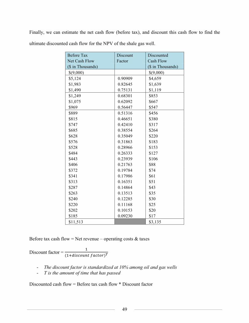
Finally, we can estimate the net cash flow (before tax), and discount this cash flow to find the
ultimate discounted cash flow for the NPV of the shale gas well.
Before Tax Discount Discounted Net Cash Flow Factor Cash Flow ($ in Thousands) ($ in Thousands) $(9,000)
$(9,000)
$5,124 0.90909 $4,659 $1,983 0.82645 $1,639 $1,490 0.75131 $1,119 $1,249 0.68301 $853 $1,075 0.62092 $667 $969 0.56447 $547 $889 0.51316 $456 $815 0.46651 $380 $747 0.42410 $317 $685 0.38554 $264 $628 0.35049 $220 $576 0.31863 $183 $528 0.28966 $153 $484 0.26333 $127 $443 0.23939 $106 $406 0.21763 $88 $372 0.19784 $74 $341 0.17986 $61 $313 0.16351 $51 $287 0.14864 $43 $263 0.13513 $35 $240 0.12285 $30 $220 0.11168 $25 $202 0.10153 $20 $185 0.09230 $17 $11,513 $3,135
Before tax cash flow = Net revenue – operating costs & taxes
Discount factor = !
(!!!"#$%&'( !"#$%&)!
- The discount factor is standardized at 10% among oil and gas wells - T is the amount of time that has passed
Discounted cash flow = Before tax cash flow * Discount factor

50
Compiling all this information, we are able to find the total discounted cash flow listed at
approximately $3,135,498. As a result, the Net Present Value (NPV) of this project is
$3,135,498, which means that the Haynesville Shale will generate approximately $3,135,498
“real dollars” in its 25-year lifespan. On a nominal basis, the shale is expected to generate
$11,513,474.
However, to get a more holistic view of the profitability of the well, investors and companies
would look at the well’s rate of return. This can be specified as the specific IRR of the well,
which we can find using the “= IRR” formula in excel, and setting the range as the 25-year time
horizon. By doing so, the model predicts an IRR of 19.6%. This 19.6% return can be confirmed
using the formula in the “evaluating profitability section” described above as well. This means
that the $9 million initial investment will generate a return of 19.6% on an annualized basis.
These results are relatively conservative and do not take into account so many additional profit
factors including technological change, decreasing costs, or increased productivity. In addition,
the Haynesville Shale has one of the highest construction costs and represents a lower bound in
the profitability of shale wells.
Summarized results:
IRR 19.6% NPV ($ in Thousands) 3,135.50
(The entirety of the model is shown on the next page)

51
Color:Peach
Drilling and Com
pletion Cost$9,000,000
Oper. Cost Esc. (%
/yr)0%
Royalty Interest15.0%
Gas Price Esc. (%
/yr)-1%
IRR
19.6%W
ell Spacing (Acres)
40D
iscount Factor10.0%
NPV
($ in Thousands)3,135.50
Leasehold Costs ($/Acre)
$0Production Taxes
3.0%
Gross G
asN
et Gas
Gas
Net
Operating
Operating
Before TaxD
iscountD
iscountedProduction
ProductionPrice
Revenue
Costs
Costs &
TaxesN
et Cash Flow
FactorC
ash FlowYear
BeginEnd
AverageD
ecline(M
cf/yr)(M
cf/yr)($/M
cf)($ Thousands)
$/Mcf
($ in Thousands)($ in Thousands)
($ in Thousands)-
(9,000)
$ (9,000)
$ 1
10,000
3,000
6,500
70.0%
2,372,5002,016,625
3.59
$ 7,240
$ 0.80
$ 2,115
$ 5,124
$ 0.90909
4,659
$ 2
3,000
2,100
2,550
30.0%
930,750791,138
3.55
$ 2,812
$ 0.80
$ 829
$ 1,983
$ 0.82645
1,639
$ 3
2,100
1,785
1,943
15.0%
709,013602,661
3.52
$ 2,120
$ 0.80
$ 631
$ 1,490
$ 0.75131
1,119
$ 4
1,785
1,517
1,651
15.0%
602,661512,262
3.48
$ 1,784
$ 0.80
$ 536
$ 1,249
$ 0.68301
853
$ 5
1,517
1,366
1,441
10.0%
526,106447,190
3.45
$ 1,542
$ 0.80
$ 467
$ 1,075
$ 0.62092
667
$ 6
1,366
1,270
1,318
7.0%
480,972408,826
3.41
$ 1,396
$ 0.80
$ 427
$ 969
$ 0.56447
547
$ 7
1,270
1,181
1,225
7.0%
447,304380,208
3.38
$ 1,285
$ 0.80
$ 396
$ 889
$ 0.51316
456
$ 8
1,181
1,098
1,140
7.0%
415,993353,594
3.35
$ 1,183
$ 0.80
$ 368
$ 815
$ 0.46651
380
$ 9
1,098
1,021
1,060
7.0%
386,873328,842
3.31
$ 1,089
$ 0.80
$ 342
$ 747
$ 0.42410
317
$ 10
1,021
950
986
7.0%
359,792305,823
3.28
$ 1,003
$ 0.80
$ 318
$ 685
$ 0.38554
264
$ 11
950
883
917
7.0%
334,607284,416
3.25
$ 923
$ 0.80
$ 295
$ 628
$ 0.35049
220
$ 12
883
822
853
7.0%
311,184264,507
3.21
$ 850
$ 0.80
$ 274
$ 576
$ 0.31863
183
$ 13
822
764
793
7.0%
289,401245,991
3.18
$ 783
$ 0.80
$ 255
$ 528
$ 0.28966
153
$ 14
764
711
737
7.0%
269,143228,772
3.15
$ 721
$ 0.80
$ 237
$ 484
$ 0.26333
127
$ 15
711
661
686
7.0%
250,303212,758
3.12
$ 664
$ 0.80
$ 220
$ 443
$ 0.23939
106
$ 16
661
615
638
7.0%
232,782197,865
3.09
$ 611
$ 0.80
$ 205
$ 406
$ 0.21763
88
$ 17
615
572
593
7.0%
216,487184,014
3.06
$ 562
$ 0.80
$ 190
$ 372
$ 0.19784
74
$ 18
572
532
552
7.0%
201,333171,133
3.03
$ 518
$ 0.80
$ 177
$ 341
$ 0.17986
61
$ 19
532
494
513
7.0%
187,240159,154
3.00
$ 477
$ 0.80
$ 164
$ 313
$ 0.16351
51
$ 20
494
460
477
7.0%
174,133148,013
2.97
$ 439
$ 0.80
$ 152
$ 287
$ 0.14864
43
$ 21
460
428
444
7.0%
161,944137,652
2.94
$ 404
$ 0.80
$ 142
$ 263
$ 0.13513
35
$ 22
428
398
413
7.0%
150,608128,016
2.91
$ 372
$ 0.80
$ 132
$ 240
$ 0.12285
30
$ 23
398
370
384
7.0%
140,065119,055
2.88
$ 343
$ 0.80
$ 122
$ 220
$ 0.11168
25
$ 24
370
344
357
7.0%
130,261110,721
2.85
$ 315
$ 0.80
$ 114
$ 202
$ 0.10153
20
$ 25
344
320
332
7.0%
121,142102,971
2.82
$ 290
$ 0.80
$ 106
$ 185
$ 0.09230
17
$ E.U
.R10,402,597
29,727$
9,214$
11,513.474$
3,135.498$
Daily Production R
ate (MC
F)
Input Variables
Hydraulic Fracturing M
odelG
as Only W
ell - Haynesville Exam
ple

52
Sensitivity Analysis In evaluating the productivity and economic profitability of any shale well, there are always
factors that fluctuate, thereby impacting the IRR and NPV values of the shale formation. The
biggest factor that fluctuates in energy production are the price of natural gas (gas price $/Mcf).
In our model, we estimated a natural gas price based on historic trading values over the past 5
years. To create a sensitivity table, we will look at a broad range of natural gas prices, adjust for
them in the model, and analyze the IRR and NPV values.
Gas Price ($/Mcf) IRR NPV (in thousands) $4.30 31.0% 6,467.87 $4.10 27.7% 5,529.17 $3.90 24.4% 4,590.48 $3.70 21.3% 3,651.78 $3.50 18.3% 2173.09 $3.30 15.3% 1,774.39 $3.10 12.5% 835.70 $2.90 9.7% -103.00
From our sensitivity analysis, the breakeven point for the producer is at a gas price of ~2.922
($/Mcf). We assumed that all other factors in the fracturing model stayed constant including
daily production rate, decline rate, and gas price deceleration for the 25-year period. Since this
data was obtained from the expected value of numerous shale formations, they will not vary
drastically from well to well. Although gas prices may fall past this point in current
commodities trading, we expect that in the long run, these prices will return to the normalized
amounts. We also have not accounted for decreasing drilling and completion costs in our model.
Changes in technology should lead to cheaper costs moving forward. As a result, we assumed
that decreases in gas prices offset the changes in drilling and completion costs to some degree.

53
From our data, as long as the long run price does not fall below $3.00, natural gas companies
have the necessary resources to withstand increased regulatory measures. The results of a
sensitivity analysis on increased drilling and completion costs are shown below:
Initial Costs (in thousands) IRR NPV (in thousands) 13,000 8.3% -864.5 12,000 10.3% 135.50 11,000 12.7% 1,135.50 10,000 15.8% 2,135.50 9,000 19.6% 3,135.50 8,000 24.7% 4,135.50 7,000 31.6% 5,135.50
Therefore, at our predicted levels, natural gas companies have almost $3 million in excess costs
that would need to be realized in order for hydraulic fracturing to be unprofitable. In addition,
by implementing additional costs, regulators create larger barriers to entry for many individual
and independent fracturing companies. By doing so, the government would inherently limit
supply and thereby increase the natural gas price. However, doing so would result in decreased
competition, and less opportunity for reducing costs and advancing technology in the hydraulic
fracturing industry. Regardless, hydraulic fracturing can be seen as an economically profitable
industry. In the following sections, we assert that there should be a federally regulated hydraulic
fracturing initiative (similar to the construction precautions of the Haynesville Shale) to regulate
the environmental impacts and the negative externalities of hydraulic fracturing.

54
Environmental Repercussions of Hydraulic Fracturing
When companies begin hydraulic fracturing, it is impossible to ignore the environmental effects
of blasting chemically-treated water through the shale layer. Fracking has taken a large toll on
the environment around the wells as well as long-term effects on the global environment. The
primary environmental effects of fracking are categorized into three sections: greenhouse gasses,
water use, and water contamination.

55
Greenhouse gasses
Source: EPA
One of the appeals of shale gas comes from the current growing amounts of greenhouse gasses.
Roughly 82% of total greenhouse gas emissions are energy-related (Jenner 2013). Natural gasses
are a great substitute for coal, although it is not currently going to directly impact transportation
due to the largely not-electric transportation industry. However, this gas can be used for heating
and other sources of energy.

56
GHG metric Specification CO2 CH4
Tropospheric concentrationa Pre-1750 280.0 700
(CO2: ppm, other: ppb) As of 2000 388.5 1870
Lifetimeb (years) 100 12
Source: Jenner 2013
Methane is a major byproduct of shale drilling from different steps of the process. First, some of
the chemicals that were mixed in with the water release methane when the water comes back to
the surface. Then, the drill out phase will leak methane as well (Jenner 2013). Additionally,
methane can seep into the water supply system nearby if cementing is not done properly around
the pipe.
Right now, roughly 3.6-7.9% of the lifetime production of a shale gas well is vented or leaked
into the atmosphere via wellhead, pipelines, and/or storage facilities, as compared with the 1.7-
6% in conventional gas wells (Jenner 2013). The best way to decrease leakage is to be more
thorough with the technology used to capture gas in the 2-week flowback period after the
fracking happens.
Water use Each well that fracking companies use requires 2-5 million gallons of water, which is 50-100x
more water than used during the extraction of conventional gas (Jenner 2013). The Haynesville
shale uses roughly 3.58 million gallons of water per drill (Nicot 2012). In order to unlock the
gas from inside the earth, companies have to learn to manage this water waste.

57
The water used in each shale gas well is in no way prepared to be reused between drillings until
it is filtered. By approximation, if we assume that the Haynesville shale uses 3.58 million gallons
of water per drill, we can calculate how much time and money it would cost to filter the water to
be used again. A company called Saltworks Technology did a case study in 2012 about how to
treat this used shale water. This toxic water must also be stored and transported to later sites in
order to be used again. Currently, roughly 70% of injected water is used in future drillings
(Pickett 2009).
An alternative to the extremely rigorous filtration process is to produce the fracturing fluids
naturally via soy and palm oil, thereby reducing the chemical additives added into the fluid.
Currently, some fracturing fluids were found to be liquified carbon dioxide and petroleum rather
than water (Jenner 2013). These are some potential alternatives to the massive amounts of water
that are used for fracking, but there is still no option that is easily replaceable.
Water contamination When blasting this chemically-infused water into the ground, up to 75% of it will come back up.
This water is now not only chemically-infused, but has picked up potentially toxic minerals from
underground. This is known as flowback water. Flowback water is laden with different
chemicals used to help the process of fracking go more smoothly: chemicals to protect the pipe,
chemicals to keep the fluid intact during immense pressure, and many salts from underground.
However, if proper measures of cementing are taken, this water should not be leaking out of the
system: the water should be easily stored and later transported.

58
Source: https://fracfocus.org/hydraulic-fracturing-how-it-works/casing
A large issue for why flowback water happens is due to the cementing process. The cementing
process is used to fill the gap between the gas pipe and the wall of the well with concrete, thus
preventing gas from coming up along the sides of the pipe and then contaminating the
groundwater. Additionally, if this cementing is not done properly, the actual flowback water
could come through the sides of the pipe due to the pressure. Another issue with policy
surrounding fracking is that cementing is not officially part of the fracking process according to
the industry’s definition, and thus is not constantly being regulated adjacent to the actual

59
fracking. It is recommended by the EPA that wells used for drinking water should be tested
before and after drilling begins at new fracking sites so as to be able to monitor flowback rates.
Proper cementing is essential to prevent groundwater contamination. The American Petroleum
Institute established the industry standard for oil and gas cementing. The first phase of cementing
begins with setting the conductor casing. This casing prevents the hole from caving into the
actual well. Next, surface casing is put in from the surface to right above the bottom of the well’s
hole. Cement is then poured down the inside of the casing, to create an annulus – the space
between the surface casing and the actual well. It is important to fill this annulus with more
cement by circulating water and cement through the annular space. Cementing happens as
companies continue to drill: cementing different layers happens as companies drill deeper into
the ground.
Furthermore, since companies now not only drill vertically, but are also drilling horizontally
within the layer of shale, scientists have recently found an issue of “fracture communication,”
where wells that are not related end up connecting underground. This has happened once with
wells that were more than 2,000 feet apart in British Columbia. The British Columbia Oil and
Gas Commission explained that weaknesses in the rock layers vary between region, and certain
areas are more likely to deteriorate the entire layer if the wells are placed too closely together
(Mooney 2011).
The risks of fracking to drinking water were researched and published by the EPA in early 2015.
The EPA discovered that contamination of drinking water does affect local neighborhoods where

60
fracking wells exist. However, the conclusion was that generally there were events that caused
the contamination, they were rarely just seeping into flowback water. The majority of the
examples occurred when fracking fluids or chemicals spilled on or near a well rather than inside
of it, and these chemicals seeped into local drinking water sources. The EPA concluded there
was not a systemic drinking water contamination problem, but rather a lack of consistency
between different wells and sources of fracking (Banerjee 2015).
Water contamination continues to be a problem for not only for drinking water but also for local
agriculture. Flowback water can easily travel and become an issue with regard to animals on
farms and irrigation. Some examples that were brought to attention include high methane levels
detected in groundwater within a 1-kilometer around the location of fracking sites (Jenner 2013).
These issues show us that flowback water is one of the most crucial things to regulate when
beginning to draft our policy proposal.
Costs of Environmental Factors Importantly we want to consider not only what the environmental impacts are, but also the cost
of these impacts. When analyzing these factors, it’s important to notice that numbers are
calculated using the Haynesville Shale, which uses more water to frack a well than average. This
produces larger values for costs, giving us more conservative estimates about general policies.

61
Social Costs of Greenhouse Gasses According to a 2010 EPA analysis on greenhouse gasses, the social cost of carbon emissions was
roughly $370 to $2,000 for one metric ton of CH4. The significantly higher bound of the social
cost estimates for an additional ton of CH4 for N2O in 2010 relative to CO2 are due to the
significantly larger radioactive forces generated by these gasses. Our paper and analysis is based
on a 2013 model, and thus we use the higher estimate of $2,000 for CH4 emission cost
calculations.
Taking into consideration the inflation rate from 2010 to 2013 of 7%:
$2,000 ∗ 1.07 ! = $2,450.09
Thus, we see a social cost of roughly $2,450 per metric ton of CH4.
Water Filtration Costs One of the larger environmental issues of fracking is the sheer amount of water needed to frack a
well once. The Haynesville Shale uses roughly 3.58 million gallons of water to frack a well
once. This water is a mixture of water, chemicals, and minerals put together by the companies
operating out of the Haynesville Shale. The liquid picks up a lot of toxins when it is injected into
the shale. Therefore, in order for this water to be reused in the next fracking procedure, the liquid
needs to be filtered.
The cost to filter the water to be used in the next fracking procedure is dependent on a few
different factors, primarily the company filtering the water. We found that the average filtration
costs for frackable water is roughly $15/m3 (Saltwater Works).

62
Thus, we convert the 3.58 million gallons into m3 and multiply by $15:
13,551.774 × 15 = $203,265
However, it is important to note that this water no longer has to be transported out of the site for
disposal, so we can subtract the cost of transporting the contaminated water assuming cost is
$5/m3:
$203,265− 13,551.774×$5 = $135,510
As we can see, the cost to filter the amount of water needed for just one cycle of fracking a well
is quite high. This process will also take roughly 100 days to properly filter.
Water Cementing Costs Lastly, one of the environmental costs of fracking is cementing and casing. The important thing
to note here is that proper cementing and casing has a lot to do with the quality of cement used
and the process of cementing (as outlined earlier).
After researching proper cementing, we see that it takes roughly $1.15 million to properly
cement and case one well, with routine check ups for fissures or changes in the well (Jenner
2013).

63
Policy Proposal
Based on the results from our economic model, we have shown that hydraulic fracturing is
economically viable even with the incorporation of environmental costs such as greenhouse gas
emissions and water filtration. We believe that there should be regulation of hydraulic fracturing
on a federal level in order to allow companies in each state to engage in horizontal drilling, both
on public and private land, with specific environmental regulations that allow gas companies to
still be profitable. The federal policy would maintain that states have jurisdiction over drilling on
private and state-owned land, and these federal regulations would serve as rules for public lands
and as a standard for state legislatures that do not have regulations. It would require companies
to publicly disclose the chemicals used in the fracturing process within 30 days of completing
fracturing operations. The federal policy would set safety standards for how companies should
store used fracking chemicals around well sites. The policy would also require companies to
submit detailed information on well geology. Lastly, it would make cementing an official part of
the hydraulic fracturing process and regulate it according the oil and gas cementing standard
established by the American Petroleum Institute to prevent groundwater contamination.

64
Conclusion and Further Discussion
By having a comprehensive set of policies on the federal level for hydraulic fracturing, we can
mitigate the negative externalities associated with the fracking process. The set of policies would
increase costs for the industry by creating higher barriers to entry and ensuring that the
environment is not harmed in fracturing process. However, as technology changes and advances,
companies in the natural gas extraction industry will still be economically profitable.
Moving forward, it will be interesting to see how the state of Illinois fares with hydraulic
fracturing. In the past, fracking companies have had a tough time setting up wells due to
legislation against the practice. However, after many years of debate and study, fracking is
expected to begin in southern Illinois in the near future. The laws written for the state establish
some of the strictest guidelines in the country. For example, every well in Illinois will need a
permit ensuring that it is properly installed. Testing of water quality near wells will be done
before and after operations. There are also regulations that require the sealing of wells and
restoration of well locations to prevent companies from just leaving the land untouched after they
have extracted the gas (NIU Newsroom 2015). Currently, there are only two energy firms who
have registered for hydraulic fracturing in Illinois – Kimmeridge Tri-State Exploration and
Denver-based Strata-x Energy – since the Illinois rules were enacted in 2014. However, drillers
have been slow to move into the state as a result of low oil prices and the extended regulatory
battles. If these two companies can make a profit, they will show that even amongst heavy
regulations, hydraulic fracturing is an economically viable industry that is worth investing in.

65
It is evident that fracking poses many risks. However, natural gas has not risen in demand quite
yet. Natural gas is currently seen as an alternative to traditional forms of gas – and a more
plentiful resource. The strict policies enacted in Illinois show the United States’ dedication to
taking steps towards a more sustainable economic model. Yet, with changes in demand for the
supply of natural gas, we can anticipate that the profits will encourage companies to enter the
more regulated market.

66
Works Referenced "10-K." SEC Filings. Halliburton, 24 Feb. 2015. Web. Anderson, Richard. "How American Energy Independence Could Change the World." BBC
News. N.p., 3 Apr. 2014. Web. 23 Nov. 2015. "Annual Energy Outlook 2015." Independent Statistics and Analysis. U.S. Energy Information
Administration, 14 Apr. 2015. Web. Auty, Richard M. "The Political Economy of Resource-driven Growth." European Economic
Review 45.4-6 (2001): 839-46. Web. Baihly, Jason. "Study Assesses Shale Decline Rates." The American Oil and Gas Reporter
(2011): n. pag. Web. Banerjee, Neela. "Fracking Has Contaminated Drinking Water, EPA Now Concludes."
InsideClimate News. Inside Climate News, 5 June 2015. Web. Barth, Jannette M. "The Economic Impact of Shale Gas Development on State and Local
Economies: Benefits, Costs, and Uncertainties." NEW SOLUTIONS: A Journal of Environmental and Occupational Health Policy 23.1 (2013): 85-101. Web.
"Country Comparison: Natural Gas - Production." Central Intelligence Agency. Central
Intelligence Agency, n.d. Web. Curtis, John B. "PGC Reports Increase in Magnitude of U.S. Natural Gas Resource Base." Press
Release. Potential Gas Committee, 8 Apr. 2015. Web. Dix, Manfred, and Greg Albrecht. "An Economic Impact Analysis of the Haynesville Shale
Natural Gas Exploration, Drilling and Production." (n.d.): n. pag. Department of Natural Resources. State of Louisiana, 28 Aug. 2008. Web.
“Drilling into complexities of fracking in Illinois”. Northern Illinois University Newsroom. 28
January 2015. Web. Earthworks, 2010. Coalition calls on New York state legislature to enact moratorium on natural
gas development. Press Release. "Economic Nature and Significance of Oil and Gas Industry." Series on Chinese Economics
Research Opening Up China's Markets of Crude Oil and Petroleum Products Theoretical Research and Reform Solutions (2014): 1-23. LaFarge. PBWCE. Web.
Engelder, Terry. "Should Fracking Stop?" Nature. Macmillin Publishers Limited, 15 Sept. 2011.
Web.

67
Feilden, Sandy. "RBN Energy." Mr. Sandman – Getting Proppant to the Wellhead. RBN Energy
LLC, 1 Aug. 2003. Web. Fielden, Sandy. RBN Production Economics Model. Shale Gas Production Economics
Spreadsheet Model. RBN Energy LLC, 19 Sept. 2013. Web. Guo, Boyun, William C. Lyons, and Ali Ghalambor. "Production Decline Analysis." Petroleum
Production Engineering (2007): 97-105. Infohost. New Mexico Tech. Web. "Haynesville Shale." Louisiana Oil Gas Association. N.p., n.d. Web. 23 Nov. 2015. Howarth, Robert W., Anthony Ingraffea, and Terry Engelder. "Natural Gas: Should Fracking
Stop?" Nature 477.7364 (2011): 271-75. Web. "How Much Should You Pay For Your Gas?" Natural Gas Royalty Estimation. Geology.com,
n.d. Web. "Independent Statistics and Analysis." Short-Term Energy Outlook. U.S. Energy Information
Administration, Nov. 2015. Web. Institute for Energy Research. "Haynesville Shale Fact Sheet." Haynesville Shale Fact Sheet
(n.d.): n. pag. 1 Jan. 2013. Web. 23 Nov. 2015. "Is Fracking a Good Idea?" Debate Club. US News, n.d. Web. Jacoby, Henry D., Francis M. O'sullivan, and Sergey Paltsev. "The Influence of Shale Gas on
U.S. Energy and Environmental Policy." Economics of Energy & Environmental Policy EEEP 1.1 (2012): n. pag. Web.
Kaiser, Mark, and Yunke Yu. "North Louisiana Drilling Costs Vary Slightly for 2007-12."
Haynesville Update. Oil and Gas Journal, 2 Dec. 2013. Web. Katz, Joseph. "How Much Does It Cost to Drill a Single Marcellus Well? $7.6M." Marcellus
Drilling News. Marcellus Drilling News, 07 Sept. 2011. Web. King, Hobart. "Uses of Natural Gas." Natural Gas Uses: Electric Power, Industry, Vehicles,
Homes. N.p., n.d. Web. 03 Dec. 2015. Krupa, Joel. "The Oil and Gas Industry: A Nontechnical Guide." Energy Policy 57 (2013): 644-
45. Web. "Measure, Manage, Maximize." Industry Leading Benchmarking, Powerful Results. Solomon
Associates, n.d. Web.

68
Miller, Thomas P., comp. "A Guide To Careers In the Oil and Gas Industry." (n.d.): n. pag. 1 Jan. 2013. Web. 23 Nov. 2015.
Mooney, Chris. "The Truth about Fracking." Sci Am Scientific American 305.5 (2011): 80-85.
Web. "Natural Gas Futures Prices (NYMEX)." Natural Gas. U.S. Energy Information Administration,
2 Dec. 2015. Web. Nicot, Jean-Philippe, and Bridget R. Scanlon. "Water Use for Shale-Gas Production in Texas,
U.S." Environmental Science & Technology Environ. Sci. Technol. 46.6 (2012): 3580-586. Web.
Ouadfeul, Sid-Ali, and Leila Aliouane. "Wellbore Stability in Shale Gas Reservoirs, A Case
Study FromThe Barnett Shale." SPE North Africa Technical Conference and Exhibition (2015): n. pag. Saltworks. Saltworks Technologies Inc., May 2014. Web.
Penner, Eric. "The Truth Is Out There – Shale Gas Production Economics Model Results." Web
log post. RBN Energy LLC, 19 Sept. 2013. Web. Perry, Kent. "Hydraulic Fracturing – A Historical and Impact Perspective." Natural Gas.
RPSEA, 18 Nov. 2010. Web. Pickett, A., 2009. New Solutions Emerging to Treat and Recycle Water Used in Hydraulic Fracs.
American Oil and Gas Reporter, March. Rohan. ""Fracking Fluid & Chemicals Market by Chemical Function (Acid, Surfactant, Biocide,
Gelling Agent, Crosslinker, Breaker, Scale & Corrosion Inhibitor, Clay & Iron Control, And Friction Reducer), by Fluid Type, & by Well Type - Global Forecasts to 2020"" Press Releases. Markets and Markets, n.d. Web.
Sachs, Jeffrey, and Andrew Warner. "Natural Resource Abundance and Economic Growth."
(1995): n. pag. Web. Scott, Loren C. The Economic Impact of the Haynesville Shale on the Louisiana Economy in
2008. Department of Natural Resources. State of Louisiana, 2009. Web. 23 Nov. 2015. Scott, Loren C. The Economic Impact of the Haynesville Shale on the Louisiana Economy in
2009. LOGA. Louisiana Oil and Gas Association, 2009. Web. 23 Nov. 2015. Scott, Loren C. The Economic Impact of the Horizontal Well Severance Tax Investment
Incentive. LOGA. Louisiana Oil and Gas Association, Mar. 2011. Web. 23 Nov. 2015. Soraghan, M., 2010a. Natural gas company’s disclosure decision could change fracking debate.
New York Times, July 15. Web.

69
Sovacool, Benjamin K. "Cornucopia or Curse? Reviewing the Costs and Benefits of Shale Gas Hydraulic Fracturing (fracking)." Renewable and Sustainable Energy Reviews 37 (2014): 249-64. Web.
Steffen, Jenner, and Alberto Lamadrid. "Shale Gas vs. Coal: Policy Implications from
Environmental Impact Comparisons of Shale Gas, Conventional Gas, and Coal on Air, Water, and Land in the United States." Energy Policy 53 (2013): 442-53. Shale Gas vs. Coal: Policy Implications from Environmental Impact Comparisons of Shale Gas, Conventional Gas, and Coal on Air, Water, and Land in the United States. Elsevier B.V., Feb. 2013. Web.
US Department of Energy: “Modern Shale Gas Development in the United States: A Primer,”
US Department of Energy, 2009 "U.S. Dry Natural Gas Production (Million Cubic Feet)." U.S. Dry Natural Gas Production
(Million Cubic Feet). U.S. Energy Information Administration, 30 Nov. 2013. Web. U.S. EPA. Assessment of the Potential Impacts of Hydraulic Fracturing for Oil and Gas on
Drinking Water Resources (External Review Draft). U.S. Environmental Protection Agency, Washington, DC, EPA/600/R-15/047, 2015.
"U.S. Natural Gas Gross Withdrawals and Production." U.S. Natural Gas Gross Withdrawals
and Production. US Department of Energy, 31 July 2015. Web. "USGS FAQs - Hydraulic Fracturing ("Fracking") - How Much Water Does the Typical
Hydraulically Fractured Well Require?" Hydraulic Fracturing ("Fracking") - How Much Water Does the Typical Hydraulically Fractured Well Require? USGS, n.d. Web.
Wood, Laura. "Fracking Fluid & Chemicals Market 2015- Global Forecasts to 2020: Major
Players in the $32 Billion Industry Are Halliburton, Schlumberger, Baker Hughes, DuPont, AkzoNobel, BASF & Ashland." Research and Markets. PR Newswire Association LLC, 12 Oct. 2015. Web.
Zeller, T., 2010. New York governor vetoes fracking bill. New York Times, December 11.