Human Development Traps and Economic Growth - ResearchGate

Electoral Studies,Vol. 17, No. 3, pp. 301–326, 1998Pergamon 1998 Elsevier Science Ltd. All rights reserved

Printed in Great Britain0261-3794/98 $19.00+0.00

PII: S0261-3794(98)00035-3

Electoral Continuity and Change, 1868–1996

Larry M. Bartels

Department of Politics and Woodrow Wilson School of Public and International Affairs,Princeton University, Princeton NJ 08544-1013, USA. E-mail: [email protected]

This article examines theoretical and historical issues raised by Donald Stokes’sclassic 1960s articles on “Party Loyalty and the Likelihood of Deviating Elections,”“On the Existence of Forces Restoring Party Competition,” and “Parties and theNationalization of Electoral Forces.” I use presidential election returns from 1868 to1996 and a simple regression model to measure partisan, national, and sub-nationalforces in each election. My analysis suggests that the contemporary American elec-toral system is significantly more nationalized than the electoral system of a centuryago, but no less partisan, no more volatile, and no less subject to competitive reequili-bration. 1998 Elsevier Science Ltd. All rights reserved

Keywords: critical elections, electoral volatility, national forces, partisanship, U.S.presidential elections

Electoral Continuity and Change, 1868–19961

Confronted with the limited configurations of the present, the survey analyst willmore and more be tempted to search for similar phenomena in the nearer and fartherpast. Far from being necessarily antihistorical, as they are sometimes supposed to be,survey studies can provide a fresh stimulus to historical analysis. (Campbellet al.,1966, 159)

The study of electoral politics has been revolutionized in the last fifty years by the avail-ability of massive amounts of high-quality survey data providing unprecedented access to theattitudes and perceptions of prospective voters. Much of that information has been gatheredby the authors ofThe American Voter(Campbellet al., 1960) and by their successors in whathave come to be called the American National Election Studies. Not surprisingly, easy scholarlyaccess to this treasure-trove of data has done a great deal to shape the contours of the field.The modern scholarly literature on electoral politics is primarily about presidential electionsrather than state and local races (or primary elections, or elections in other political systems),primarily about individual political psychology rather than elite behavior or mass-elite linkages,primarily about voting behavior rather than aggregate election outcomes, and primarily aboutthe present rather than the past—all, at least in significant part, because that is where the bestdata are.

276 Electoral Continuity and Change, 1868–1996

While this scholarly development has produced an unusually rich and technically sophisti-cated body of political research, it has also encouraged a sort of provincialism, in which thetotality of electoral politics is sometimes too readily equated with the psychology of votingbehavior in the dozen U.S. presidential elections since 1952. Apparent changes within thisfairly narrow compass are taken as reflections of momentous social or political transformations,while apparent continuities are taken as evidence of the way things have always been and willalways be. What is one to make of a scholarly literature in which successive decades havewitnessed the unveiling ofThe American Voter(Campbellet al., 1960),The Changing Amer-ican Voter(Nie et al., 1976),The Unchanging American Voter(Smith, 1989), andThe NewAmerican Voter(Miller and Shanks, 1996)?

In view of these developments, it is well worth recalling that the authors ofThe AmericanVoter—and Donald Stokes perhaps foremost among them—clearly recognized the limitationsof the contemporary survey data on which their classic work was based, and strove in a varietyof ingenious ways to produce a more complete and nuanced understanding of electoral politicsthan could be afforded by those data alone. Their efforts to extend the scope of electoralresearch beyond the reach of national opinion surveys are reflected in the cross-national collab-orations of Campbell and Valen and of Converse and Dupeux (both reprinted in Campbelletal., 1966), in the classic works on representation by Miller and Stokes (also reprinted inCampbellet al., 1966), and in Stokes’s work with David Butler on the British political system(Butler and Stokes, 1969); they are also reflected in a somewhat different way in the seriesof historical essays by Stokes considered here, which represent the core of his scholarship inthe decade separatingThe American Voterin 1960 andPolitical Change in Britainin 1969.2

Within two years after the publication ofThe American Voter, Stokes was consciouslyattempting to project the framework and findings of that work onto a broader canvas. “Thecontemporary voting studies,” he wrote (Stokes, 1962, 689),

have disposed of many questions whose answers could only be guessed a few yearsago. Yet any such cumulation of findings brings to the fore a number of ‘second-generation’ problems that could hardly be stated except in terms of the theoreticalideas evolving out of current work. This has especially been true in the voting studiesas interest has extended from the population of voters to a population of elections;concepts that could explain a good deal about individual choice inevitably spawnedadditional questions about elections as total social or political events.

Given the limitations of contemporary survey data, an interest in ‘elections as total socialor political events’ impelled Stokes to examine the historical record of aggregated electoraldata, primarily but not only in the United States. In the process, he organized previouslyfugitive election returns,3 developed innovative statistical models and methods for analyzinghistorical electoral data,4 and played a major role in defining as well as resolving the ‘second-generation’ problems" posed for the broader field of electoral studies by the findings of contem-porary survey research.

My aim here is to revisit the issues of electoral continuity and change raised by Stokes inthree important works from this period (Stokes, 1962; Stokes and Iversen, 1962; Stokes, 1967),applying models and methods he would (I like to think) have applied himself had he writtenthese works thirty years later, and using the intervening thirty years’ data both to shedadditional light on the broad sweep of American electoral history and to shed some light onour current political circumstances. That the specific questions Stokes formulated seem astheoretically and historically relevant in the 1990s as they did in the 1960s is, I submit, atestament to his remarkable intellectual vision.

277Larry M. Bartels

Components of the Vote

The data for my analysis consist of state-level presidential election returns for the 33 electionsfrom 1868 through 1996.5 I focus here on the Republican popular vote margin in each state,defined as the difference between the Republican and Democratic percentages of the total votecast for president. I prefer this measure to the Republican share of the two-party vote becausethe latter measure tends to overstate the winning party’s dominance in elections with strongthird-party showings.6

I make no concerted effort to analyze support for third-party and independent candidates,largely because that support has been so sporadic and ephemeral in the period covered by myanalysis. The total vote cast for candidates other than the Republican and Democratic nomineeshas averaged only five percent in these 33 elections, and the half-dozen cases in which itreached ten percent or more (1912, 1992, 1924, 1968, 1892, and 1996) have displayed ratherlittle continuity in voting patterns.7

The Republican vote margins in the 33 presidential elections from 1868 through 1996 areshown as dots in Fig. 1. The figure also shows a moving average through time of the individualelection outcomes, which provides a clearer visual representation of historical shifts in partydominance.8 By this moving average measure, the Republican party was dominant (at thepresidential level) from the Civil War until the accession of Franklin Roosevelt, and againfrom Eisenhower through Bush—albeit at times only narrowly, and with reversals in specificelections, most spectacularly in 1912 and 1964. It is also interesting to note, however, thatdespite these long periods of Republican dominance, the median vote margin is exactly zero,and 20 of the 33 margins are smaller than ten percentage points.

The election outcome in each state in each election year may usefully be thought of as asum of three distinct components: a partisan component reflecting standing loyalties carryingover from previous elections, an election-specific component reflecting the shifting tides ofnational electoral forces, and an idiosyncratic component reflecting new sub-national electoralforces at work in the specific state. I propose to measure these three distinct components ofthe vote by regressing state election outcomes in each election year on previous election out-comes in the same state plus a constant. The regression model is

Rst = at + b1tRst − 1 + b2tRst − 2 + b3tRst − 3 + est, (1)

whereRst represents the Republican vote margin in states in election yeart, andRst−1, Rst−2,and Rst−3 represent the Republican vote margins in the same state in the three immediatelypreceding elections.at, b1t, b2t, andb3t are election-specific parameters to be estimated, andest is a stochastic term reflecting state-specific idiosyncratic forces in election yeart; I willassume for purposes of estimation thatest is drawn from a probability distribution with meanzero and election-specific variancest

2.The parameters of this regression model correspond directly to the three components of the

vote distinguished here: the parametersb1t, b2t, andb3t on lagged state votes reflect standingpartisan loyalties carrying over from previous elections, the intercept parameterat measuresthe overall vote shift attributable to national electoral forces in a given election, and the stochas-tic variance parameterst

2 measures the magnitude of new sub-national forces in a given elec-tion.

Estimates of these parameters for each of the 33 presidential elections examined here arepresented in Table 1. Each row of the table represents one regression, with the number of


Fig. 1. Election outcomes, 1868–1996

observations corresponding to the number of states voting in that election year.9 In order toreflect national voting behavior, all of the data are weighted by the number of votes cast in eachstate in each election year, so that more populous states receive more weight in the regressions.

The first column of Table 1 shows the square root of the estimated stochastic variance ofsub-national forces in each election year (st ) in percentage points; the second column showsthe estimated national partisan swing (at ) in percentage points (with positive values indicatingRepublican swings, negative values indicating Democratic swings, and standard errors of theestimates in parentheses); the third, fourth, and fifth columns show the estimated persistenceof previous state-level outcomes in each election year (b1t, b2t, andb3t); and the sixth columnshows the sum of these three lagged partisan effects (again, with its standard error inparentheses).10

For example, the parameter estimates for the 1996 election presented in the first row ofTable 1 show that the state-level voting pattern in 1996 basically replicated the pattern in 1992,

279Larry M. Bartels

Table 1. Components of the Presidential Vote, 1868–1996

st (Sub- at ΣbtElection b1t b2t b3tNational (National (PartisanYear (4-year Lag) (8-year Lag) (12-year Lag)Forces) Forces) Loyalties)

1996 5.755 −5.198 (3.610) 1.087 (0.187)−0.060 (0.184) 0.164 (0.178) 1.191 (0.092)1992 4.518 −15.664 (1.963) 0.404 (0.153) 0.379 (0.191)−0.016 (0.097) 0.767 (0.073)1988 4.298 −9.975 (1.491) 1.085 (0.088)−0.240 (0.135)−0.085 (0.119) 0.760 (0.074)1984 3.884 1.026 (1.345) 0.582 (0.101)−0.029 (0.109) 0.467 (0.044) 1.020 (0.071)1980 5.233 9.991 (1.797) 0.742 (0.098) 0.036 (0.074) 0.322 (0.114) 1.100 (0.095)1976 7.658 2.871 (4.636)−0.274 (0.132) 0.712 (0.134)−0.043 (0.087) 0.395 (0.107)1972 8.141 30.323 (2.366) 0.686 (0.229) 0.356 (0.086)−0.324 (0.225) 0.717 (0.144)1968 5.293 6.250 (1.295) 0.234 (0.058) 0.782 (0.102) 0.009 (0.091) 1.024 (0.122)1964 12.613 −7.988 (3.111) 0.927 (0.299)−0.708 (0.283)−0.385 (0.355)−0.165 (0.234)1960 6.444 −3.435 (2.058) −0.350 (0.142) 0.798 (0.138)−0.019 (0.094) 0.429 (0.097)1956 6.683 10.572 (2.123) 0.595 (0.122) 0.123 (0.109) 0.098 (0.087) 0.816 (0.104)1952 8.311 14.679 (1.532) 0.101 (0.136) 0.488 (0.367)−0.101 (0.329) 0.488 (0.111)1948 8.555 2.078 (3.432) 0.104 (0.394) 0.207 (0.361) 0.136 (0.179) 0.446 (0.089)1944 3.269 2.368 (1.406) 0.820 (0.061) 0.055 (0.095) 0.004 (0.056) 0.879 (0.031)1940 7.703 10.841 (3.124) 1.113 (0.159)−0.189 (0.136) 0.193 (0.083) 1.117 (0.089)1936 7.388 −12.256 (3.663) 0.703 (0.099)−0.030 (0.088) 0.021 (0.080) 0.694 (0.077)1932 10.683 −28.393 (3.100)−0.150 (0.147) 1.070 (0.215)−0.496 (0.210) 0.424 (0.129)1928 10.751 13.994 (4.381) 0.976 (0.164) 0.767 (0.202) 0.047 (0.178) 0.257 (0.090)1924 9.851 3.675 (5.181) 0.879 (0.127) 0.144 (0.174) 0.134 (0.150) 1.157 (0.098)1920 9.480 19.478 (4.250) 0.249 (0.184) 0.046 (0.160) 0.904 (0.187) 1.200 (0.093)1916 8.105 −3.216 (3.644) 0.247 (0.124) 0.946 (0.176)−0.192 (0.121) 1.001 (0.080)1912 9.832 −25.556 (2.014) 0.557 (0.270) 0.049 (0.144) 0.083 (0.252) 0.689 (0.095)1908 5.678 −1.383 (1.212) 0.311 (0.095) 0.620 (0.206) 0.028 (0.083) 0.958 (0.062)1904 8.192 9.864 (1.499) 1.617 (0.204)−0.446 (0.123) 0.291 (0.107) 1.462 (0.080)1900 5.726 3.171 (0.994) 0.471 (0.058) 0.079 (0.130) 0.504 (0.202) 1.053 (0.074)1896 16.688 4.130 (2.866)−0.825 (0.335) 2.573 (0.719)−0.648 (0.630) 1.100 (0.206)1892 8.273 −2.798 (1.376) 1.167 (0.271)−0.289 (0.370) 0.243 (0.200) 1.121 (0.101)1888 4.923 −2.124 (0.900) 1.019 (0.146) 0.392 (0.181)−0.395 (0.148) 1.016 (0.063)1884 6.032 1.022 (2.019) 0.764 (0.171) 0.069 (0.217)−0.117 (0.116) 0.715 (0.070)1880 6.294 6.863 (2.075) 1.112 (0.142)−0.357 (0.126) 0.096 (0.075) 0.851 (0.084)1876 4.765 −7.501 (1.706) 0.541 (0.103) 0.230 (0.131) 0.009 (0.106) 0.780 (0.082)1872 7.295 6.712 (2.318) 0.428 (0.192)−0.151 (0.188) 0.365 (0.091) 0.642 (0.117)1868 6.410 −2.286 (2.077) 0.740 (0.104) 0.136 (0.075) 0.235 (0.072) 1.111 (0.110)

but with an across-the-board shift of five percentage points toward Clinton. (The national shiftis reflected in the intercept of−5.198, while the stability of relative support from 1992 to 1996is reflected in a coefficient close to one for four-year lagged votes and coefficients close tozero for eight-year lagged votes and twelve-year lagged votes.) Sub-national forces are capturedby the standard error of this regression, which gauges the extent to which the 1996 outcomein specific states deviated from the overall pattern. (For example, Clinton did notably worsein Kansas—Robert Dole’s home state—in 1996 than in 1992, and considerably better in severalnortheastern states than the overall regression relationship would suggest.) The estimated mag-nitude of these sub-national forces was slightly larger in 1996 than in the previous four electioncycles, but smaller than in most of the elections before 1980.

The results presented in Table 1 provide the basis for the analyses in the next three sectionsof this paper, each focusing on a single aspect of American electoral history. The first of these


sections deals with the persistence of partisan loyalties, the second with the magnitudes ofnational and sub-national electoral forces, and the third with the identification of ‘critical elec-tions.’ Subsequent sections on the dynamics of party competition and on the volatility ofelection outcomes are based upon national-level rather than state-level analysis of the sameelection returns.

The Persistence of Partisan Loyalties

One of the most widely accepted generalizations in the whole scholarly literature on votingbehavior and elections is that party loyalties count for less in contemporary American politicsthan they did a generation or more ago. For example, Wattenberg (1990, 1991) has used datafrom the National Election Studies and other sources to documentThe Decline of AmericanPolitical PartiesandThe Rise of Candidate-Centered Politics, while Burnham (1989, 24) hasreferred more colorfully to ‘a massive decay of partisan electoral linkages’ and to ‘the ruinsof the traditional partisan regime.’ These developments have sometimes been taken to implythat the whole theoretical framework presented inThe American Voter, with its emphasis onthe causal priority of long-standing partisan loyalties, has become increasingly irrelevant inthe contemporary American context.

Characteristically, Stokes expressed curiosity about the extent and causes of temporal andspatial variation in the strength of party identification even before contemporary survey databegan to register noticeable departures from the levels of partisanship documented inTheAmerican Voter. ‘The reality which parties have as objects of mass perception,’ he wrote(Stokes, 1967, 183),

is the more remarkable in view of the actual fragmentation of party structure and thediffusion of authority produced on all levels of government by the doctrine of separ-ated powers. Indeed, the ambiguity of parties as stimulus objects suggests that thefocus of partisan attitudes may vary a good deal and that the modern American experi-ence may differ from that of other liberal democracies or earlier periods of ourown politics.

Lacking direct measures of party identification from contemporary surveys in most ‘otherliberal democracies or earlier periods of our own politics,’ it seemed reasonable to Stokes—and still seems reasonable today—to look for evidence of party loyalties in the continuity ofpartisan voting patterns over time. To the extent that successive elections with different candi-dates, issues, and political conditions produce essentially similar voting patterns, it seems safeto infer that these patterns somehow reflect the organizing force of partisanship. Of course,whether that organizing force is manifested through party machines, party symbols, parentalsocialization, or other specific mechanisms may vary from time to time and place to place,and the mere fact of continuity does nothing to illuminate the actual workings of the relevantelectoral processes. Nevertheless, the mere fact of continuity in partisan voting patterns oversignificant periods of timedoesseem to provideprima facieevidence of the importance ofpartisanship in one form or another.

The logic of this inference is nicely captured by Stokes (1962, 691) own example:

we may suppose that any one judging the candidates according to the dominant valuesof American culture, rather than in purely partisan terms, would have found GroverCleveland a more estimable man than James G. Blaine in the campaign of 1884. Yetwe can be sure that the public’s actual response to these new presidential personalities

281Larry M. Bartels

was colored almost completely by its prior partisan loyalties, as the smallness of thevote swing from 1880 to 1884 suggests.

Of course, the national vote swing from one election to the next might be small for a varietyof reasons having little to do with the public’s partisan loyalties. For example, positiveresponses to Cleveland’s personality in some parts of the country might (despite Stokes’sassessment of the candidates) have been counterbalanced by positive responses to Blaine’spersonality in other regions, or by defections from the Democratic platform planks on silver,regulation, or other policy issues of the day. However, the same pattern of countervailingelection-specific deviations would be much less likely to occur simultaneously in each statethan in the nation as a whole. Thus, the fact that more than three-quarters of each state’spartisan popular vote margin in the election of 1880 persisted in the election of 1884—despitethe intervening assassination of President Garfield, the recession of 1884, and the emergenceof Cleveland and Blaine as their parties’ nominees—seems to provide considerable supportfor Stokes’s inference that voters’ responses to the immediate candidates and issues werestrongly colored by their partisan loyalties. Nor is Stokes’s example historically atypical; theestimates of lagged partisan effects for 11 of the 32 other elections in Table 1 are even larger,and theaveragecombined effect of the three most recent past elections (in the last columnof Table 1) for the entire 130-year time span is 0.825. Clearly, party loyalties have produceda good deal of continuity in presidential voting patterns at many points in American elec-toral history.

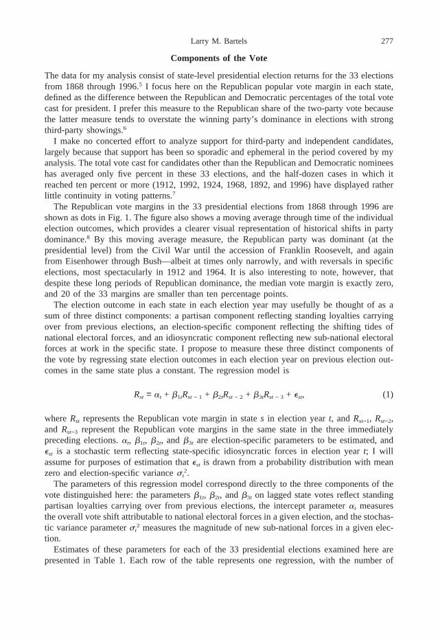
While the magnitude of partisan effects evident in Table 1 is impressive, the variability ofthese effects is also impressive. There is far more election-specific variation in the estimatedstrengths of party loyalties than could be attributed to random fluctuation in the parameterestimates themselves. The historical evolution underlying this election-specific variation is indi-cated by the locally weighted regression trend line drawn through the plotted party loyaltyestimates (the sums of 4-year, 8-year, and 12-year lagged effects from the last column of Table1) in Fig. 2.

Two aspects of the historical evolution shown in Fig. 2 may be surprising. First, the persist-ence of partisan loyalties appears to have declined throughout the first half of the 20th centuryfrom the very high level of the Gilded Age. The first half of this decline is largely attributableto the election of 1912, in which a long-standing Republican majority was fractured by thesplit between William Howard Taft and Theodore Roosevelt. However, the second half of thedecline reflects a series of elections in the New Deal era in which pre-existing partisan loyaltieswere significantly eroded. The first two of these, in 1928 and 1932, mark the end of theProgressive era party system and the beginning of the New Deal era itself. Whereas the electionof 1896 superimposed new sub-national forces on a basically stable party system (as evidencedby estimated partisan persistence levels in Table 1 of 1.12 in 1892, 1.10 in 1896, 1.05 in 1900,and 1.46 in 1904), the New Deal realignment erased much of the existing party system (asevidenced by estimated partisan persistence levels of 0.26 in 1928, 0.42 in 1932, and 0.69 in1936). Moreover, what Sundquist (1983) has referred to as the aftershocks of the New Deal,especially in the South, produced a great deal of further reshuffling in 1948, 1952, 1960, 1964,and 1976 (with estimated partisan persistence levels of 0.45, 0.49, 0.43,− 0.16, and 0.40,respectively). It seems fruitless to argue about which one of these elections marked the endof the New Deal party system, when the evidence suggests that the system was in considerablepartisan flux almost throughout its existence.

The other potentially surprising feature of the historical evolution graphed in Fig. 2 is the


Fig. 2. Partisan forces, 1868–1996

notable resurgence of partisan forces in the last 20 years. The five most recent presidentialelections have been characterized by a persistence of party loyalties unsurpassed over anycomparable time span since the turn of the last century. The strong correlation between state-level election returns in 1984 and 1988 adduced by Bartels (1992) to illustrate the continuingrelevance of party identification in presidential elections appears from the parameter estimatespresented in Table 1 to be fairly typical of the whole period. Whatever prospective voters maysay in response to survey questions, and whatever academics may write and believe, actualpresidential election outcomes suggest that we have been living through an era marked byunusually strong partisan continuity in state-level voting patterns.

The revival of partisanship evident in Fig. 2 is even more striking in Fig. 3, which tracksthe persistence of partisan voting patterns outside the South.11 Whereas Fig. 2 shows a fairlysteady decline in the persistence of partisan voting patterns through the first six decades ofthe twentieth century, Fig. 3 shows a shorter and sharper decline, followed by a longer and

283Larry M. Bartels

Fig. 3. Partisan forces, Non-south

even more impressive increase in the strength of partisan forces over the last sixty years. Thedifference between these patterns reflects the fact that Democratic loyalties in the ‘Solid South’survived the New Deal realignment intact, but began to erode significantly in the 1950s and1960s, when the rest of the country was already in a period of historically typical partisanpersistence. It seems clear, however, that the unusually high- and still increasing-levels ofpartisan persistence in recent presidential elections are no mere artifact of the breakup of theSolid South, since they appear clearly even in an analysis limited to non-southern states.

National and Local Forces

Stokes’s interest in ‘Parties and the Nationalization of Electoral Forces’ stemmed primarilyfrom his interests in legislative behavior and political representation. “Many influences affectthe solidarity of a legislative party,” he wrote (Stokes, 1967, 184),


but the members’ perception of forces on their constituents’ voting behavior is surelyamong them.... If the member of the legislature believes, on the one hand, that it isthe national party and its leaders which are salient and that his own electoral prospectsdepend on the legislative record of the party as a whole, his bonds to the legislativeparty will be relatively strong. This is the situation posited by the model of responsibleparty government. But if the legislator believes, on the other hand, that the public isdominated by constituency influences and that his prospects depend on his own orhis opponent’s appeal or on other factors distinctive to the constituency, his bondsto the legislative party will be relatively weak.

Stokes set out to measure the influence of national and local forces on turnout and votingbehavior in legislative elections, not only in the contemporary United States, but over a 90-year span of American history (from the 1870s through the 1950s) and in Britain as well. Hefound a substantial and fairly regular decline in constituency-specific variation in turnout incongressional elections, and a somewhat later decline (first evident in the 1930s) in localinfluences on the partisan vote division in congressional races. “If the nationalization of polit-ical forces has carried less far in America than in Britain,” he concluded (Stokes, 1967, 202),“it seems nevertheless an outstanding aspect of our elections for Congress over the life of themodern party system.”

My own historical analysis of presidential election returns allows for a roughly parallelanalysis of changes over time in the extent to which voting behavior has been dominated bynational or local forces. Indeed, the absence of cross-sectional variation in the identity of thecompeting candidates makes presidential elections especially useful for gauging changes in theextent to which the electorate itself has become more or less homogeneous in its voting behavi-or.

A natural measure of the magnitude of national forces in presidential elections is the absolutevalue of theat coefficient reflecting overall shifts in the presidential vote in each election year.These absolute values are charted in Fig. 4. The three highest values shown in the figure, eachcorresponding to a national vote shift of 25 to 30 percentage points, represent the Republicandebacle of 1912, the repudiation of Herbert Hoover in 1932, and the Nixon landslide of 1972.The national vote shift in a typical election year is, of course, much smaller in magnitude—about nine percentage points. Even this modest historical average was not reached in any ofthe nine elections between 1868 and 1900. However, the magnitude of national forces increasedmarkedly over the first three decades of the 20th century, reaching a peak at the beginning ofthe New Deal era before subsiding to a fairly consistent average of ten percentage points forthe remainder of the century.

An equally natural measure of the magnitude of sub-national forces in each election yearis the standard deviationst of state-specific political shocks. These sub-national forces, graphedin Fig. 5, display much less temporal variation than the national forces graphed in Fig. 4.There are notable outliers of 17 percentage points in 1896 and 13 percentage points in 1964,but relatively constant averages of eight percentage points over the whole period from 1868through 1928 and seven percentage points over the whole period from 1932 through 1996. Itis interesting to note that the pattern of local forces in presidential elections shown in Fig. 5is roughly similar to the pattern Stokes (1967) 195, found in congressional elections, with agradual increase from the 1870s into the 1920s followed by a decline from the 1920s throughthe 1940s. It is also interesting to note that the eight most recent elections have clustered nearthe lower end of the historical distribution, suggesting that the decline in the magnitude ofsub-national effects may have resumed in the last twenty years.

285Larry M. Bartels

Fig. 4. National forces, 1868–1996

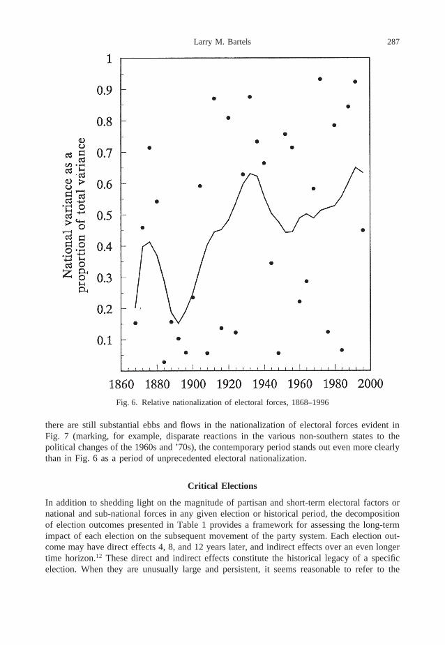
The national and sub-national forces charted in Figs 4 and 5, respectively, are directly com-parable in the sense that both are measured on the same scale of percentage point changes inthe popular vote. Thus, it is possible not only to assess fluctuations in the magnitude of eachforce over the 13 decades covered by the figures, but also to assess the relative magnitude ofnational and sub-national forces at any given point, in much the way Stokes (1967) did forcongressional and British parliamentary elections. Fig. 6 displays the relative magnitude ofnational forces—represented by the ratio of national variance (the square of the national tidecoefficient at in Table 1) to national variance plus sub-national variance (the square of thestate-specific shock coefficientst in Table 1)—in each election year.

The pattern of relative nationalization in Fig. 6 suggests that national and sub-national forceshave been relatively evenly balanced throughout most of this century, but with the balancetipping toward national forces at the beginning of the New Deal and in the most recent electionsand toward sub-national forces during the racial sorting-out of the 1950s and ’60s. By contrast,


Fig. 5. Sub-National forces, 1869–1996

sub-national forces were predominant through most of the late 19th century, with nationalvariance exceeding sub-national variance in only two of the first nine elections shown in Fig.6. On a broad historical scale, Fig. 6 might be read as a reflection of long-term nationalizationof the mass media and of American political culture more generally. However, the notablereversals of this long-term trend evident in the 1880s and ’90s and again during the New Dealera suggest that technological and social forces producing greater nationalization have, at leastat times, been stymied by deep sectional political cleavages.

The political significance of the most important such sectional cleavage is evident fromcomparing the pattern of nationalization in Fig. 6 with the corresponding pattern in Fig. 7,which is based upon parallel calculations of national and sub-national forces derived fromregression analyses omitting the southern states. The general pattern in Fig. 7 suggests a moreconsistent nationalizing trend than in Fig. 6, with the trough following Reconstruction and thepeak marking the advent of the New Deal party system both considerably smoothed. While

287Larry M. Bartels

Fig. 6. Relative nationalization of electoral forces, 1868–1996

there are still substantial ebbs and flows in the nationalization of electoral forces evident inFig. 7 (marking, for example, disparate reactions in the various non-southern states to thepolitical changes of the 1960s and ’70s), the contemporary period stands out even more clearlythan in Fig. 6 as a period of unprecedented electoral nationalization.

Critical Elections

In addition to shedding light on the magnitude of partisan and short-term electoral factors ornational and sub-national forces in any given election or historical period, the decompositionof election outcomes presented in Table 1 provides a framework for assessing the long-termimpact of each election on the subsequent movement of the party system. Each election out-come may have direct effects 4, 8, and 12 years later, and indirect effects over an even longertime horizon.12 These direct and indirect effects constitute the historical legacy of a specificelection. When they are unusually large and persistent, it seems reasonable to refer to the


Fig. 7. Relative nationalization of electoral forces, Non-south

election as a ‘critical election’ in the sense developed by Key (1955, 1959), Burnham (1970),Sundquist (1983), and others.

My calculation of the long-term impact of each election takes into account the magnitudeof new national and sub-national forces in that election (reflected by the estimates ofat andst, respectively, in Table 1) as well as the persistence of those forces in subsequent elections(reflected by the estimates ofb1t, b2t, and b3t for subsequent elections in Table 1). Morespecifically, I average the immediate impact of new national and sub-national forces in eachelection (represented by the square root of the sum ofat

2 andst2), the direct impact four years

later (consisting of the immediate impact multiplied byb1t + 1), the total impact eight yearslater (consisting of the immediate impact multiplied byb2t + 2 plus the fourth-year impactmultiplied by b1t + 2) and so on, over a total of seven elections spanning a quarter-century.13

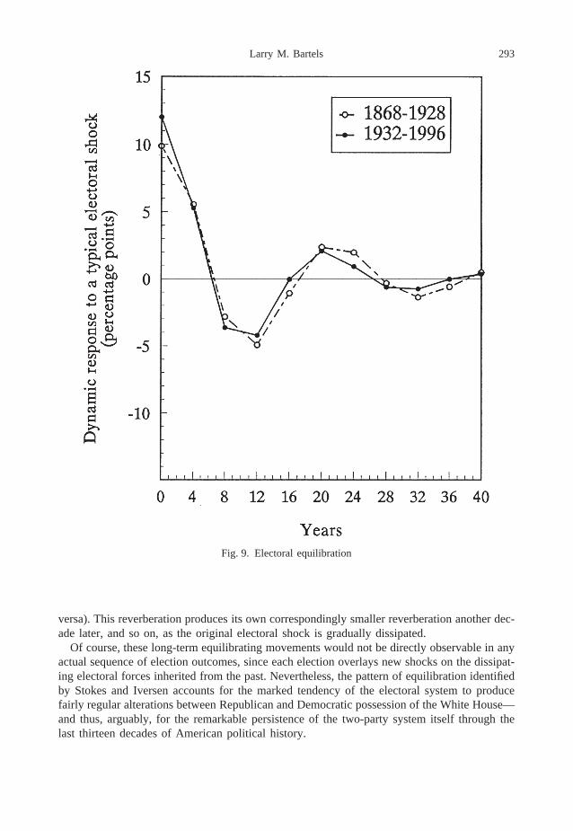
The long-term effects calculated in this manner for each election from 1868 to 1972 are shownin Fig. 8, which displays the average impact of each election over a 24-year horizon.14

289Larry M. Bartels

Fig. 8. Critical elections, 1868–1972

The estimates of the long-term impact of each election represented in Fig. 8 conform insome respects to expectations derived from the scholarly literature on critical elections. Mostobviously, the election of 1932 stands out as the most influential single election of the entire100-year period, with an average impact over a quarter-century of more than 15 percentagepoints. This was a critical election by any reasonable standard, and the calculation on whichFig. 8 is based nicely captures that fact.

In some other respects, however, the results presented in Fig. 8 must be regarded as stronglycounterintuitive. For one thing, the distribution of long-term effects seems a good deal morediverse than one would expect from a scholarly literature so strongly fixated on the electoralsignificance of a handful of critical elections. Rather than consisting of a few great peaksseparated by broad plateaus reflecting long periods of political stasis, the distribution of long-term effects in Fig. 8 reflects a complex intermixture of large, medium and small effects.15

What is more, the long-term importance attached to specific presidential elections in Fig. 8is in several cases quite out of keeping with the estimates of previous political observers. A


sense of the nature and bases of these discrepancies may be provided by considering in somedetail two specific elections. One of these, the election of 1896, has been considered “one ofthe decisive elections in American history” by Schattschneider (1960, 76) and many subsequentanalysts. The other, the election of 1880, has not figured at all in the literature on criticalelections, but appears in Fig. 8 as the second most important election of the century followingthe Civil War.

The voting pattern of 1896 was unusual in being marked by a set of sub-national shocksmore than twice as large in magnitude as those observed on average in the other 32 electionsexamined here. These shocks reflect the regional reorientation of the party system precipitatedby the Democrats’ nomination of William Jennings Bryan on a Populist platform, which drovemuch of the industrial Northeast and Midwest strongly into the Republican camp. Thus, in animmediate sense, the election of 1896 marked an important shift in the existing party system.16

However, when we consider the combined effect of national and sub-national forces, the elec-tion of 1896 appears to have had a good deal less immediate impact than the elections of1912, 1932, or 1972, which produced less sub-national reshuffling but much larger nationalshifts;17 it ranks in immediate impact with the elections of 1920, 1928, 1936, 1952, and 1964.

This short-term calculation alone seems to shed some doubt upon the conventional classi-fication of 1896 as a critical election. However, the longer-term calculation reflected in Fig.8 sheds even more doubt upon that classification by indicating that the electoral pattern estab-lished in 1896 was much less durable than previous scholarship has suggested, despite thepersistence of the Republican majority—with one eight-year interruption—for another gener-ation. According to the calculations presented in Table 1, the electoral impetus of 1896 wasdiminished by half within four years; the state-by-state voting pattern in 1900 reflected thedivisions of 1888 (with a coefficient of 0.504) as much or more than those of 1896 (with acoefficient of 0.471). Moreover, the direct carryover of the 1896 voting pattern was actuallynegative in 1904 (with a coefficient of− 0.446), and negligible in 1908 (with a coefficient of0.028). Thus, if we focus not only on the extent to which the electoral pattern of 1896 wasdiscontinuous with those of the immediate past, but also on the extent to which the distinctiveelectoral forces that emerged in 1896 persisted into the future, it seems difficult to sustainSchattschneider’s (1960, 76) characterization of this as “one of the decisive elections in Amer-ican history.”

By contrast, the election of 1880 appears in Fig. 8 as the second most significant electionof the entire 100-year period, despite its virtual invisibility in the scholarly literature. Theimmediate impact of the election of 1880 amounted to 9.3 percentage points—about half theimmediate impact of the election of 1896, and a third that of 1932. This immediate impactwas roughly evenly divided between a national shift toward the Republicans (counteractingthe Democratic tide of 1876) and a reshuffling of sub-national voting patterns reflecting theend of Reconstruction. For example, Louisiana and South Carolina reported Republican majori-ties in 1872 and 1876, but reverted to Democratic control as soon as federal troops werewithdrawn in 1877, and supplied Democratic popular vote margins of 25 and 31 percentagepoints, respectively, in 1880. In an important sense, this was not anew partisan alignment,but a reconstitution of thestatus quo ante bellum.18

What made the election of 1880 so significant, at least by the calculations summarized inFig. 8, was not its short-run impact but the persistence of the renewed partisan cleavages itreflected. Having returned to the Democratic fold in 1880, both Louisiana and South Carolina—and most of the rest of the South—remained there for 80 years. Moreover, even outside theSouth, the period of stable partisan competition following the settlement of 1876 perpetuated

291Larry M. Bartels

the electoral pattern established in 1880 for the next three decades, despite the interventionsof populism, depression, and a colonial war. Thus, for example, while the impact of the electionof 1896 had declined by my calculations from eight percentage points in 1900 to six by 1908,the impact of the election of 1880 had nearly doubled from seven percentage points in 1884to almost 14 percentage points in 1908.

It is worth noting that the electoral pattern of 1880 persisted despite the apparent absenceof any significant ‘realigning issue.’ According to one historian (Hicks, 1949, 162),

both parties were completely bankrupt. The issues that divided them were historicalmerely.... The platforms of the two parties in 1880 revealed few real differences ofopinion as to policies and no real awareness of the problems that confronted thenation. Neither Democrats nor Republicans seemed to sense the significance of thevast transformation that was coming over business, nor the critical nature of therelationship between labor and capital, nor even the necessity of doing somethingdefinite about civil service reform, the money problem, and the tariff. The RepublicanParty existed to oppose the Democratic Party; the Democratic Party existed to opposethe Republican Party.... With issues lacking, the campaign turned on personalities.

Here, clearly, was an election bearing few of the hallmarks of the ideal-typical critical elec-tion envisioned by political scientists and historians. Nevertheless, the distinct electoral patternestablished in 1880 persisted longer and more powerfully than that of all but one of the 32other presidential elections examined here. That fact is a testament to the intensely organizedpartisan struggle of the Gilded Age, but also to the limitations of a theoretical perspective thatstrains to find in the complex historical record of partisan struggles a stately procession ofmore or less static issue-based party alignments.

The Dynamics of Party Competition

One of the most striking features of the time series of presidential election outcomes displayedin Fig. 1 is that the Republican popular vote margin never strays very far or very long fromthe competitive equilibrium represented by an even partisan division of the vote. There arefew instances of 20-point vote margins, and no instances of 30-point vote margins, in this130-year period.19 Only once has either party maintained even a 10-point vote margin for threesuccessive elections, and this impressive 8-year run (by the Republicans from 1920 to 1928)was immediately followed by the Democrats’ most impressive 8-year run (from 1932 to 1940).

In their piece ‘On the Existence of Forces Restoring Party Competition’ Stokes and Iversen(1962, 159–160) suggested a variety of possible explanations for this regularity:

Restoring forces have been seen in such diverse factors as the tendency of interestgroups to remember the favors an administration has dispensed less than the favorsit has not; the ability of the party out of power to make more flexible and extravagantpromises of future benefit whereas the party in power is limited by what it can actuallydeliver; the greater motivational strength of the public’s negative response to anadministration’s mistakes than of its positive response to an administration’s suc-cesses; the liability of the party in power to disastrous splits as its majority growsand its sense of electoral pressure lessens; movements of the business cycle, generat-ing new support for the opposition party in periods of economic decline; the alternat-ing moods of liberalism and conservatism that have marked our national temper; anda vigorous popular belief in rotation in office, which turns the peccadilloes of a partylong in power into convincing evidence that the time for a change has arrived.


Stokes and Iversen (1962) demonstrated the reality of ‘restoring forces’ by positing as analternative a non-parametric ‘random walk’ model in which the partisan division of the presi-dential vote could move in either direction with equal probability in each election, and showingthat the persistent competitiveness of observed election outcomes was extremely unlikely givensuch a model. They also noted in passing (1962, footnote 7) that “if the division of the voteat one presidential election is correlated with thechangeof the vote from that election to thenext, a negative correlation of− .55 is obtained. In other words, the greater a party’s share ofthe vote at one election, the greater is its share likely to be reduced at the next.”

My own analysis of the dynamics of party competition in presidential elections builds uponthis latter result, using the observed change in the Republican vote margin in each electionyear as the dependent variable in a regression with vote margins in the previous two electionsas explanatory variables. If equilibrating forces are at work, we should expect previous votemargins to have a negative impact on current changes in the vote margin, producing Democraticshifts following Republican victories and Republican shifts following Democratic victories.The parameter estimates reported in Table 2 clearly conform to this expectation, with eachpercentage point of the winning party’s vote margin producing direct negative effects of abouthalf a percentage point in each of the two subsequent elections.20

The second and third columns of Table 2 present comparable parameter estimates separatelyfor the periods from 1868 through 1928 and from 1932 through 1996. The separate parameterestimates for the two periods are virtually identical, suggesting that the equilibrating forcesexplored by Stokes and Iversen have persisted essentially unchanged through several gener-ations of American partisan struggles.21 Neither the replacement of traditional patronage-basedparty machines with modern media campaigns nor the vast expansion of the scope and activitiesof the federal government in the period covered by this analysis seems to have produced anysignificant alteration in the appetite or ability of losing politicians to reclaim the reigns ofgovernment through electoral competition.

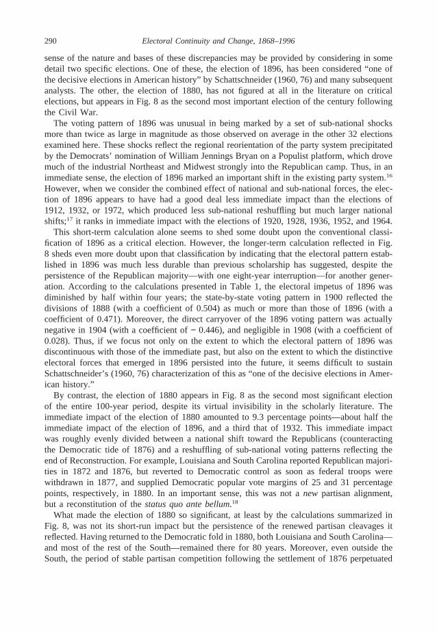
The impact of the equilibrating forces measured in Table 2 is illustrated in Fig. 9, whichtraces the implied dynamic response of the political system to a typical electoral shock in eachof the 60-year periods covered by my analysis. Here, too, the similarity of the two distinctsets of estimates is evident. In each period, half of a typical gain (or loss) of ten to twelvepercentage points in the Republican vote margin is likely to persist four years later. But inthe next two elections after that, the net effect is reversed, with Democrats actually doingnoticeablybetter than they would have in the absence of the original Republican gain (or vice

Table 2. Competitive Equilibration. Parameter estimates (with standard errors in parentheses) fromordinary regression analyses of changes in presidential vote margins (in percentage points) on previous

margins

1868–1996 1868–1928 1932–1996

Margint −4 −0.474 (0.156) −0.438 (0.234) −0.561 (0.222)Margint −8 −0.525 (0.157) −0.602 (0.261) −0.496 (0.206)Intercept 2.59 (1.98) 5.59 (2.86) −0.10 (2.94)adjusted R2 0.47 0.42 0.51std error of reg 10.90 9.88 12.00Durbin-Watson 1.97 1.97 1.60N 33 16 17

293Larry M. Bartels

Fig. 9. Electoral equilibration

versa). This reverberation produces its own correspondingly smaller reverberation another dec-ade later, and so on, as the original electoral shock is gradually dissipated.

Of course, these long-term equilibrating movements would not be directly observable in anyactual sequence of election outcomes, since each election overlays new shocks on the dissipat-ing electoral forces inherited from the past. Nevertheless, the pattern of equilibration identifiedby Stokes and Iversen accounts for the marked tendency of the electoral system to producefairly regular alterations between Republican and Democratic possession of the White House—and thus, arguably, for the remarkable persistence of the two-party system itself through thelast thirteen decades of American political history.


Electoral Volatility

Stokes’s studies of electoral politics (Stokeset al., 1958; Campbellet al., 1960; Stokes, 1962;Stokes and Iversen, 1962; Stokes, 1966; Butler and Stokes, 1969) are marked by an intenserecurring interest in the balance and interplay of long-term and short-term political forces. Ashe put it in one of those pieces (Stokes, 1962, 689–690),

By measuring a limited set of political orientations (among which party loyalty ispreeminently important) we are able to say with increasing confidence what thebehavior of the American electorate would be in any given election if the vote wereto express only the influence of these basic dispositions. But the election returnsreflect, too, the public’s reaction to more recent and transitory influences (think forthe moment of candidate personality) that deflect the vote from what it would havebeen had these short-term factors not intruded on the nation’s decision. Therefore,any national election can be thought of as an interplay of basic dispositions and short-run influences. Yet the freedom of these ‘disturbing’ influences to modify the effectsof long-term dispositions is not well understood. Their capacity to do so is not oftrivial importance; there have been few presidential elections in a hundred years thatwe could not imagine having gone to the loser, had the right combination of short-term factors appeared in time. And yet each election is not a fresh toss of the coin;like all good prejudices, the electorate’s basic dispositions have a tremendous capacityto keep people behaving in accustomed ways. The freedom of short-run influencesto deflect the vote has an obvious bearing on how well long-standing party loyaltiesare able to explain a total election outcome. Plainly, a closer estimate of the easewith which short-term electoral tides may run to one party or the other would tell agood deal about the importance of party identification in a predictive theory of elec-tions.

Stokes treated the distinction between long-term and short-term forces both as an organizingframework for survey-based research on the components of individual vote choices (Stokesetal., 1958; Stokes, 1966) and as an aggregate-level property of electoral systems. In “PartyLoyalty and the Likelihood of Deviating Elections” (Stokes, 1962), he used the observed distri-bution of presidential election outcomes around their long-term average (calculated alterna-tively from 1892 through 1928 and from 1892 through 1960) to estimate the probability ofwhat Campbellet al. (1960, 531–538) had referred to as a ‘deviating’ election.

Subsequent analysts who have argued that the long-term stabilizing force of party identifi-cation has declined substantially since the 1950s have seemed to assume as a matter of coursethat the magnitude of short-term forces has increased concomitantly, driven by the reactionsof large numbers of unanchored ‘independent’ voters to candidate images and performance.For example, Wattenberg (1991, 21) argued that ‘the focus of the campaign’ has turned “fromlong-term to short-term issues. Being less tied to the patterns of the past, the American elector-ate is far more volatile compared to three decades ago, and has grown accustomed to lookingdirectly at the candidates through the mass media.”

This perception of increased volatility was presumably fueled by the evident variability ofpresidential election outcomes since the 1950s, with substantial popular vote landslides wonby both parties (in 1964, 1972, and 1984) and only one twelve-year stretch of uninterruptedcontrol of the White House by either party (from 1981 through 1993). But how does that levelof volatility compare with the level observed at other periods in American electoral history?Fig. 10 displays the time trend of volatility in presidential elections over the entire period of

295Larry M. Bartels

Fig. 10. Electoral volatility, 1868–1996

my analysis, as measured simply by the magnitude of the national popular vote swing in eachelection—the absolute values of the changes in vote margin analyzed in Table 2.

Fig. 10 shows two clear peaks in the volatility of presidential election outcomes. One ofthese, of about twenty years’ duration, encompasses the break-up of the prevailing Republicanmajority in 1912, its reinstitution in 1920, and its replacement by the New Deal majority in1932; the second, somewhat shorter and sharper, reflects the electoral turbulence of the 1960sand ’70s, including the Goldwater and McGovern debacles in 1964 and 1972. This second peakof electoral volatility seems to confirm the widespread perception that presidential elections inthe television age have become significantly more volatile than they used to be.

Unfortunately, any such simple generalization must collapse in the face of the subsequenttime trend of electoral volatility in Fig. 10. Whereas the presidential elections of the 1960sand ’70s were highly volatile by historical standards, the five most recent presidential electionshave evidenced levels of volatilitybelow the long-run historical average. It is certainly not


true now, as it would have been in the 1970s, that “the American electorate is far more volatilecompared to three decades ago” (Wattenberg, 1991, 21). It would seem to follow that anyplausible explanation for the volatility of the 1960s and ’70s must be based upon specificfeatures of that historical period rather than secular technological or other trends.

Fig. 11 displays an alternative historical record of volatility based upon residual popular voteswings from the analysis in Table 2. This more sophisticated measure reflects the magnitude ofthe vote swing in each election net of the reequilibrating forces carrying over from previouselections. Thus, it probably provides a better estimate of the extent to which the actual electionoutcome deviated from the ‘expected’ outcome in Stokes’s sense.

Not surprisingly, the residual vote swings shown in Fig. 11 tend to be considerably smallerin magnitude than the total vote swings shown in Fig. 10. The contrasts in volatility betweenhistorical peaks and troughs are also less pronounced. However, the basic pattern in Fig. 10is essentially replicated in Fig. 11.22 The historically low volatility of the last two decades of

Fig. 11. Residual volatility, 1868–1996

297Larry M. Bartels

the 19th century and the periods of high volatility from 1912 through 1932 and in the 1960sand ’70s appear clearly in Fig. 11, just as they do in Fig. 10. The return to historically lowlevels of volatility in recent presidential elections also appears clearly in Fig. 11, reinforcingthe conclusion that the high volatility of the 1960s and ’70s was a temporary phenomenonrather than a sea change in the nature of American electoral politics.

Electoral Change in Historical Perspective

Three decades ago, Stokes (1967, 183) worried that “[t]he very richness of contemporaryAmerican survey data poses the danger that conclusions of unwarranted generality will bedrawn from the evidence at hand.” That worry seems amply justified by the results reportedhere, but in a way that Stokes might have found surprising. Rather than mistaking contemporaryAmerican political conditions for eternal regularities—as some critics ofThe American Voterand Stokes himself seem to have feared—observers have, in my view, overstated the particu-larity of contemporary political conditions while overlooking important elements of continuitywith previous eras of American electoral history.

Despite the widespread belief among political scientists that the American electoral systemis more volatile and unconstrained by partisan loyalties than ever before, systematic analysisof election returns suggests just the opposite: the unusual political turmoil of the 1960s and’70s has given way to a period of partisan stability and predictability unmatched since the endof the 19th century.

No doubt, every generation is tempted to imagine itself unique, and one of the mostimportant uses of history is to dispel the illusion that we live in an era of unprecedented thisor that. The historical questions addressed by Stokes in the works I have revisited here continueto serve that purpose very well, providing a bracing perspective on the nature of continuityand change in the American electoral system.

Notes

1. This is a revised version of a paper originally presented at the Donald Stokes memorial panel, AnnualMeeting of the American Political Science Association, Washington, DC, August 1997. I am gratefulto Princeton University and the John Simon Guggenheim Memorial Foundation for generous financialsupport for the research reported here, and to Daniel Carpenter, John Zaller, and anonymous refereesfor helpful reactions to the original version.

2. I have attempted elsewhere (Bartels, 1997) to provide a more detailed assessment of the aims andsignificance of the whole corpus of Stokes’s work on electoral politics.

3. Stokes and Iversen (1962) presented the first time series of national congressional vote percentagesgoing back to the Civil War, a forerunner of the ambitious historical data collection carried out underthe auspices of the Inter-University Consortium for Political and Social Research.

4. Stokes’s (1962) use of a normal error model and Stokes and Iversen’s (1962) use of a random walkmodel were both, to the best of my knowledge, unprecedented in political science. Later, Stokesdevoted considerable scholarly energy to addressing methodological problems arising in analyses ofaggregated data (Stokes, 1969) and developing and applying a ‘variance components’ model for whatare now commonly referred to as hierarchical data (Stokes, 1965, 1967).

5. The data are taken from Congressional Quarterly (1995), updated with 1996 returns fromCon-gressional Quarterly Weekly Report. These data are derived from Scammon and McGillivray (1994),but differ in minor respects from those compiled by Robinson (1934) and Petersen (1963).

6. Including third-party voters in the denominator, as I do, implicitly assumes that they would dividetheir support evenly between the two major candidates if forced to choose between them; excludingthird-party voters implicitly assumes that they would divide their support in the same proportions as


those who actually voted for the two major candidates. Both these assumptions are surely false, butthe first is probably closer to the truth than the second, since the major party that loses more of itsusual supporters to a strong third-party challenge is likely to lose the election, as the Republicansdid in 1912 and 1992. Most of Theodore Roosevelt’s supporters in 1912 were surely Republicans,while polling data from 1992 suggest that Ross Perot drew as much or more from George Bush asfrom Bill Clinton.

7. For example, even with Ross Perot in both the 1992 and 1996 races, the correlation between thetotal vote shares for third-party and independent candidates in those two elections was only 0.71,while the corresponding correlation between Republican vote margins in 1992 and 1996 was 0.88.Defections from the two-party system in 1996 were also correlated with previous defections in 1980(0.63), 1968 (− 0.63), 1924 (0.59), and 1912 (0.50). However, these correlations mostly reflect therelative appeal of third-party candidates in the South; the corresponding correlations for non-southernstates only are 0.23.,− 0.25, 0.35, and 0.04.

8. The moving averages shown in this and subsequent figures were generated by locally weightedregressions of election outcomes on time using theksm lowessprocedure in the Stata software pack-age. Beck and Jackman (1998) provide an introduction to locally weighted regression and relatedtechniques. All of my locally weighted regressions employ bandwidths of 0.3, meaning that 40 years’worth of data are used to calculate the summary value at each point, with temporally proximateobservations receiving more weight than those more distant in time.

9. Actually, because lagged election outcomes appear as explanatory variables in Table 1, each stateappears in the regressions twelve years after it entered (or, in the case of the former Confederatestates following the Civil War, reentered) the electorate. Thus, the number of observations rangesfrom 20 in 1868 to 51 (including the District of Columbia) since 1976.

10. The sum of the three lagged partisan effects in a given election year is often estimated more preciselythan the separate effects themselves. This fact reflects the positive correlations among the threeseparate measures of past election outcomes, which make it harder to disentangle their separateeffects but easier to measure their joint effect.

11. The calculations presented in Fig. 3 – and in Fig. 7 below – are based on regression analyses parallel-ing those reported in Table 1, but omitting data from the eleven former Confederate states.

12. In principle, the indirect effects of any given election can persist indefinitely or even increase overtime. In practice, given the magnitudes of the estimated continuity coefficients in Table 1, the effectstend to decline fairly monotonically, so that the impact of each election outcome gradually fadeswith the passage of time.

13. Thus, the seven terms in each average are;vt = (at2 + st

2)1/2, vt + 1 = b1t + 1vt, vt + 2 = b1t + 2vt + 1

+ b2t + 2vt, vt + 3 = b1t + 3vt + 2 + b2t + 3vt + 1 + b3t + 3vt, vt + 3 = b1t + 3vt + 2 + b2t + 3vt + 1 + b3t + 3vt,vt + 4 = b1t + 4vt + 3 + b2t + 4vt + 2 + b3t + 4vt + 1, vt + 5 = b1t + 5vt + 4 + b2t + 5vt + 3 + b3t + 5vt + 2,vt + 6 = b1t + 6vt + 5 + b2t + 6vt + 4 + b3t + 6vt + 3.

14. These calculations of long-term effects may be usefully contrasted with the ‘real time’ approach tothe study of political realignments developed by Cavanagh (1997). Cavanagh’s calculations usingcounty-level election returns grouped by regions are consistent with mine in suggesting that “thestability of the presidential alignment during the contemporary era from 1980–96 has attainedthehighest level in the history of the American party system”(Cavanagh, 1997, 7; emphasis in original),but his classification of realigning elections based solely on breaks from the recent past—withoutreference to their subsequent durability—produces results that look more like Sundquist’s (1983)than like those presented here.

15. In addition to flying in the face of much of the classic literature on ‘critical elections,’ these resultsstand in marked contrast to the statistical results reported by Nardulli (1995, Fig. 1) which displayclear peaks in 1896 and 1932 and lesser peaks in 1928 and 1960. However, these discrepancies mayreflect the fact that Nardulli’s (1994, 1995) analysis is based on an interrupted time-series analysisthat “requires the analyst to specify the point at which major, enduring interruptions in long-termelectoral trends (critical elections) are hypothesized to begin, as well as the form of those interrup-tions” (Nardulli, 1995, 11), whereas the approach adopted here incorporates no theoretical precon-ceptions regarding the timing or nature of critical elections.

16. This discontinuity is perhaps best captured by the simple correlation across states between the Repub-lican vote margins in 1892 and 1896: 0.43. The corresponding correlations between current andimmediately preceding vote margins from 1880 through 1892 ranged from 0.91 to 0.94, while those

299Larry M. Bartels

from 1900 through 1924 ranged from 0.80 to 0.93. In the whole data series analyzed here, thediscontinuity apparent in 1896 was only exceeded in 1960 (0.33), 1964 (0.12), and 1976 (0.02).However, even this discontinuity is somewhat more complicated than it appears at first sight; themore detailed regression analysis reported in Table 1 shows that the pattern of vote margins in 1896combined a strongnegativecarryover from 1892 (− 0.825) with an even strongerpositivecarryoverdirectly from 1888 (2.573).

17. Despite the reality of widespread Republican gains in the nation’s urban industrial areas in 1896,the Republican share of the total popular vote only increased by eight percentage points (from 43percent in 1892 to 51 percent in 1896), while the Democratic share remained almost unchanged.

18. For example, the correlation between the Republican vote margins in 1880 and 1856—for the thirtystates that participated in both elections—was 0.84. This correlation over a quarter-century exceedsmost of the correlations between adjacent elections in the whole period covered by my analysis!

19. Of course, an even longer time horizon would have included the suspension of partisan competitionat the presidential level during the Era of Good Feeling following the War of 1812.

20. Allowing for serial correlation in the residuals from this regression would leave the results virtuallyunchanged; the estimated serial correlation is 0.03 with a standard error of 0.18. The results areequally impervious to adding the vote margin 12 years earlier as an additional explanatory variable(the resulting coefficient is 0.015 with a standard error of 0.181) or adding the number of consecutiveyears the incumbent party has been in office (the resulting coefficient is− 0.111 with a standarderror of 0.243).

21. The estimated serial correlations of the stochastic disturbances are− 0.22 (with a standard error of0.26) in the pre-New Deal period and 0.10 (with a standard error of 0.22) in the post-New Dealperiod. Adjusting the analysis to allow for these serial correlations would change the estimated laggedeffects to− 0.309 (0.219) and− 0.719 (0.257) in the pre-New Deal period and− 0.635 (0.224) and− 0.491 (0.211) in the post-New Deal period. The dynamics for each period implied by these esti-mates are quite similar to those shown in Fig. 9.

22. The most notable difference between the patterns in Fig. 10 and Fig. 11 is that the periods of highelectoral volatility appear somewhat later and last somewhat longer in Fig. 11. Thus, the first majorperiod of high volatility in Fig. 11 encompasses much of the early New Deal period, as the Demo-cratic majority established in 1932 withstood for some time the usual pattern of competitive erosion;and the second major period of high volatility in the 1960s and ’70s is also slightly later and longer,since the Republican gains in 1968 and 1972 are counted in the calculations underlying Fig. 11 aspartly predictable reequilibrations following the Democratic landslide of 1964.

References

Bartels, L. M. (1992) The Impact of Electioneering in the United States. InElectioneering: A ComparativeStudy of Continuity and Change, ed. D. Butler and A. Ranney. Clarendon Press, Oxford.

Bartels, L. M. (1997) Donald Stokes and the Study of Electoral Politics.PS: Political Science and Politics30, 230–232.

Beck, N. and Jackman, S. (1998) Beyond Linearity by Default: Generalized Additive Models.AmericanJournal of Political Science42, 596–627.

Burnham, W. D. (1970)Critical Elections and the Mainsprings of American Politics. W. W. Norton,New York.

Burnham, W. D. (1989) The Reagan Heritage. InThe Election of 1988: Reports and Interpretations, ed.G. M. Pomper et al. Chatham House, Chatham, NJ.

Butler, D. and Stokes, D. (1969)Political Change in Britain: Forces Shaping Electoral Choice. St.Martin’s Press, New York.

Campbell, A., Converse, P. E., Miller, W. E. and Stokes, D. E. (1960)The American Voter. John Wileyand Sons, New York.

Campbell, A., Converse, P. E., Miller, W. E. and Stokes, D. E. (1966)Elections and the Political Order.John Wiley and Sons, New York.

Cavanagh, T. E. (1997)Assessing Realignment in Real Time: The Contemporary American Party Systemin Historical Context.Paper prepared for delivery at the annual meeting of the American PoliticalScience Association, Washington, DC.


Congressional Quarterly, 1995.Presidential Elections: 1789–1992. Congressional Quarterly Inc., Wash-ington, DC.

Hicks, J. D. (1949)The American Nation: A History of the United States from 1865 to the Present, 2nded. Houghton Mifflin Company, Boston.

Key, V. O. (1955) A Theory of Critical Elections.Journal of Politics17, 3–18.Key, V. O. (1959) Secular Realignment and the Party System.Journal of Politics21, 198–210.Miller, W. E. and Shanks, J. M. (1996)The New American Voter. Harvard University Press, Cam-

bridge, MA.Nardulli, P. F. (1994) A Normal Vote Approach to the Study of Electoral Change: Presidential Elections,

1828–1984.Political Behavior16, 467–503.Nardulli, P. F. (1995) The Concept of a Critical Realignment, Electoral Behavior, and Political Change.

American Political Science Review89, 10–22.Nie, N. H., Verba, S. and Petrocik, J. R. (1976)The Changing American Voter. Harvard University Press,

Cambridge, MA.Petersen, S. (1963)A Statistical History of the American Presidential Elections. Frederick Ungar Pub-

lishing Company, New York.Robinson, E. E. (1934)The Presidential Vote: 1896-1932. Stanford University Press, Stanford, CA.Scammon, R. M. and McGillivray, A. V. (1994)America at the Polls. Congressional Quarterly, Wash-

ington, DC.Schattschneider, E. E. (1960)The Semisovereign People: A Realist’s View of Democracy in America.

Harcourt Brace Jovanovich, 1975, Fort Worth.Smith, E. R. A. N. (1989)The Unchanging American Voter. University of California Press, Berkeley, CA.Stokes, D. E. (1962) Party Loyalty and the Likelihood of Deviating Elections.Journal of Politics24,

689–702. Reprinted inElections and the Political Order, A. Campbell, P. E. Converse, W. E. Miller,and D. E. Stokes. John Wiley and Sons, 1966, New York.

Stokes, D. E. (1965) A Variance Components Model of Political Effects. InMathematical Applicationsin Political Science, ed. J. M. Claunch. Arnold Foundation, Dallas.

Stokes, D. E. (1966) Some Dynamic Elements of Contests for the Presidency.American Political ScienceReview60, 19–28.

Stokes, D. E. (1967) Parties and the Nationalization of Electoral Forces. InThe American Party Systems:Stages of Political Development, ed. W. N. Chambers and W. D. Burnham. Oxford University Press,New York.

Stokes, D. E. (1969) Cross-Level Inference as a Game against Nature. InMathematical Applications inPolitical Science IV, ed. J. L. Bernd. University Press of Virginia, Charlottesville, VA.

Stokes, D. E., Campbell, A. and Miller, W. E. (1958) Components of Electoral Decision.AmericanPolitical Science Review52, 367–387.

Stokes, D. E. and Iversen, G. R. (1962) On the Existence of Forces Restoring Party Competition.PublicOpinion Quarterly26, 159–171. Reprinted inElections and the Political Order, A. Campbell, P. E.Converse, W. E. Miller, and D. E. Stokes. John Wiley and Sons, 1966, New York.

Sundquist, J. L. (1983)Dynamics of the Party System: Alignment and Realignment of Political Partiesin the United States, revised ed. Brookings Institution, Washington, DC.

Wattenberg, M. P. (1990)The Decline of American Political Parties: 1952–1988. Harvard UniversityPress, Cambridge, MA.

Wattenberg, M. P. (1991)The Rise of Candidate-Centered Politics: Presidential Elections of the 1980s.Harvard University Press, Cambridge, MA.

Documents

Human Development Traps and Economic Growth - ResearchGate