Embed Size (px)
Citation preview

Human Capital Response to Globalization: Education
and Information Technology in India
Gauri Kartini Shastry�
Wellesley College
This draft: March 2011; First draft: October 2007
Abstract
Recent studies show that trade liberalization increases skilled wage premiums indeveloping countries. This result suggests globalization bene�ts skilled workers morethan unskilled workers, increasing inequality. However, if human capital investmentresponds to new global opportunities, this e¤ect may be mitigated. I study how theimpact of globalization varies across Indian districts with di¤erent costs of skill acqui-sition. I focus on the relative cost of learning English versus Hindi, since English isuseful for high-skilled export jobs. Linguistic diversity in India compels individualsto learn either English or Hindi as a lingua franca. Some districts have lower relativecosts of learning English due to linguistic predispositions and psychic costs associatedwith past nationalistic pressure to adopt Hindi. I demonstrate that districts where itis relatively easier to learn English bene�t more from globalization: they experiencegreater growth in both information technology jobs and school enrollment. Consistentwith a larger human capital response, they experience smaller increases in skilled wagepremiums. Keywords: education, India, outsourcing. JEL Codes: O, I, F.
�Correspondence: [email protected]. I am grateful to Shawn Cole, David Cutler, Esther Du�o,Caroline Hoxby, Lakshmi Iyer, Patrick McEwan, Asim Khwaja, Michael Kremer, Sendhil Mullainathan andRohini Pande for their advice and comments, Aimee Chin, Petia Topalova and David Clingingsmith for helpwith the data and seminars participants at various institutions. I thank the Warburg Funds Research Grantsat Harvard University for �nancial support to collect the data and the Dissertation Internship at the Boardof Governors of the Federal Reserve System for �nancial support. The views expressed here are mine anddo not necessarily re�ect those of any of these institutions. In addition, I thank Elias Bruegmann, FilipeCampante, Davin Chor, Quoc-Anh Do, Eyal Dvir, Alex Gelber, Li Han, C. Kirabo Jackson, Michael Katz,Katharine Sims, Erin Strumpf and Daniel Tortorice for helpful conversations. All errors are mine.

1 Introduction
Recent literature suggests that trade liberalization in poor countries, particularly in Latin
America, increases skilled wage premiums, a common indicator of inequality.1 These results
are not predicted by a simple Heckscher-Ohlin model,2 and there are multiple explanations
for this divergence. Some explanations focus on global outsourcing (Feenstra and Hanson
1996, 1997) and complementarities between skill levels (Kremer and Maskin 2006).3 A
key, understudied factor in understanding the e¤ects of globalization, however, is the supply
response of human capital. If the supply of skilled workers rises (as in East Asia, but less so in
Latin America4), this may drive down the skilled wage premium and mitigate globalization�s
e¤ect on inequality.
I examine this issue in Indian districts with plausibly di¤erent supply elasticities. Some
districts have a more elastic supply of English language human capital, particularly relevant
for service exports. I show that these districts attracted more export-oriented skilled jobs,
speci�cally in information technology (IT),5 and experienced greater growth in schooling.
Consistent with this factor supply response, these districts experienced smaller growth in
skilled wage premiums.
I study trade liberalization in India in the early 1990s. Motivated by a balance-of-
payments crisis, reforms reduced trade barriers and removed restrictions on private and
foreign direct investment. While this shock was common across India, historical linguistic
forces created di¤erences in the ability of districts to take advantage of new global opportu-
nities. I examine how the impact of globalization varied with these pre-existing di¤erences.
1See Goldberg and Pavcnik (2004) for a review of the literature, which focuses on Latin America (e.g.Hanson and Harrison 1999; Feenstra and Hanson 1997; Feliciano 1993; Cragg and Epelbaum 1996; Robbins,Gonzales and Menendez 1995; Robbins 1995a, 1995b, 1996b, 1996a; Attanasio, Goldberg and Pavcnik 2004;Robbins and Gindling 1997). There is little evidence on East Asia, but conventional wisdom suggests asmaller e¤ect. See Wood (1997), Lindert and Williamson (2001) and Wei and Wu (2001).
2In a two-good, two-country Heckscher-Ohlin model, a labor-abundant poor country should specialize inunskilled labor intensive industries, increasing demand for unskilled workers and lowering wage premiums.
3Additional explanations are discussed in Goldberg and Pavcnik (2004).4See Attanasio and Szekely (2000), Sanchez-Paramo and Schady (2003).5IT refers to both software and business process outsourcing such as call centers and data entry �rms.
1

Speci�cally, I show that the e¤ect of liberalization varies with the elasticity of human
capital supply by exploiting exogenous variation in the cost of learning English. Some vari-
ation is naturally endogenous: state governments that care more about trade opportunities
may also promote English instruction. Instead, I use exogenous variation, produced by his-
torical linguistic diversity, that spurred people to learn English even in 1961, long before
the 1990s trade reforms. The variation stems from substantial local linguistic diversity that
motivates individuals to learn a lingua franca,6 either English or Hindi. Individuals whose
mother tongues are linguistically further from Hindi have a lower relative opportunity cost
of learning English: they �nd Hindi more costly to learn and speak, relative to people whose
mother tongues are linguistically similar to Hindi. Using several de�nitions of linguistic dis-
tance, I demonstrate that distance from Hindi induces people to learn English and schools
to teach English. Because of considerable local linguistic diversity, I am able to rely purely
on pre-existing, local variation, minimizing concerns that variation in linguistic distance is
correlated with unobserved geographic di¤erences.7
Using new data on the Indian information technology sector, I �rst show that IT �rms
were more likely to operate where costs of learning English are lower. My choice of the IT
sector is driven by several factors. The industry grew primarily due to trade liberalization
and technological progress. Exports make up 82% of the median �rm�s revenue. In addition,
IT �rms almost exclusively hire English speakers; data on other jobs that require English is
unavailable.8 I use this industry as a proxy for new global export opportunities.9
Next, I demonstrate that districts with languages further from Hindi experienced greater
increases in school enrollment from 1993 to 2002 relative to prior trends. These districts
also had greater enrollment growth in English than local languages in 2002-2007. Finally,
6A lingua franca is a language used as a common or commercial language among diverse linguistic groups.7I take out regional or state-level variation with the appropriate �xed e¤ects. The six regions in India
each consist of 2-7 states, each of which is made up of 1-51 districts.8A search for �English�on an Indian job website (PowerJobs) delivered mostly ads in IT, but also postings
for teachers, engineers, receptionists, secretaries, marketing executives and human resources professionalsthat required English �uency. Many of these jobs are in multinational or exporting �rms.
9See Topalova (2004, 2005) for the e¤ect of import competition on productivity and poverty in India
2

using individual-level data, I show that these districts experienced a smaller increase in
the skilled wage premium. This di¤erence in the relative increases in schooling and skilled
wage premiums is evidence that the supply response of human capital shapes the impact of
globalization. Solely demand-driven explanations for the increase in skill acquisition would
predict a greater increase in both education and the skilled wage premium.
I do not claim that the impacts on education and wages are driven entirely by IT; the
IT industry is only a fraction of export-related, English-language opportunities. My results
on schooling and wages are likely to be driven by all global opportunities. Because of the
importance of English to these �rms and in my identi�cation strategy, I believe these results
are driven by global opportunities and not integration within the Indian economy which
might also have occurred during this period. I discuss this claim further in section 6.
This paper contributes to a growing literature on globalization, language and education.
Levinsohn (2004) examines how globalization in South Africa increases the returns to English.
Ku and Zussman (2010) �nd that English pro�ciency promotes trade between countries
with di¤erent native languages. Using household data from Mumbai, India, Munshi and
Rosenzweig (2006) �nd increases in the returns to English and enrollment in English-medium
schools from 1980 to 2000. Azam, Chin and Prakash (2010) estimate large returns to English
in India. Jensen (2011) demonstrates that providing recruiting services to help rural women
get jobs in IT reduces the gender gap in investments in children�s human capital. Oster and
Millett (2010) demonstrate that school enrollment in villages close to where call centers are
located increases faster than in other villages in three states in India and that this e¤ect is
larger for schools that teach in English. The authors include school �xed e¤ects, but do not
explain the call centers�location decisions. Finally, Edmonds, Pavcnik and Topalova (2007)
�nd that import competition increases poverty and reduces schooling.
The paper is organized as follows. Section 2 describes trade liberalization and IT in India
while section 3 develops a simple theoretical framework. Section 4 describes the Indian
linguistic context. In section 5, I discuss the empirical strategy. Section 6 presents the
3
results on IT �rm presence, school enrollment growth and returns to education and section
7 provides a discussion of robustness checks. Section 8 concludes.
2 Background on trade liberalization and IT
India has traditionally controlled its economy and limited trade through investment li-
censing and import controls. Since the late 1970s, the government took small steps towards
liberalization, but even as late as 1990, numerous obstacles blocked trade. A balance-of-
payments crisis in 1991 precipitated a shift towards an open economy. Reforms ended most
import licensing requirements for capital goods and cut tari¤s. The March 1992 Export-
Import Policy reduced the number of goods banned for export from 185 to 16. From 439
goods subject to some control, the new regime limited only 296 exports. The government
relaxed capital controls, particularly for exporters, and devalued the rupee, further reducing
deterrents to trade (Panagariya 2004).
Services in particular had been heavily regulated. State-owned enterprises dominated in-
surance, banking, telecommunications and infrastructure. The reforms in the 1990s opened
these sectors to private participation and foreign investment. The 1994 National Telecommu-
nications Policy opened cellular and other telephone services, previously a state monopoly,
to both private and foreign investors. Due to technological progress, this policy was reaf-
�rmed in 1999 under the New Telecom Policy which further reduced limits on foreign direct
investment (FDI) in telecommunications. FDI for internet service providers was permitted
with few limitations. FDI in e-commerce, software and electronics was granted automatic
approval, particularly for IT exporters (Panagariya 2004). Note that liberalization was at a
national level and reforms did not di¤er in areas with many English speakers.
These reforms led to remarkable growth in exports; annual growth rose 3.3 percentage
points in the 1990s from the 1980s. Service exports grew more rapidly than manufacturing
exports; even within manufacturing, skilled labor intensive sectors grew faster (Panagariya
4

2004). This policy shift, along with technological progress, led to the growth of IT services
outsourced to India. By 2004, India was the single largest destination for foreign �rms seeking
IT services. IT outsourcing accounted for 5% of India�s GDP in 2005 (Economist 2006).
Employment growth was strong: from 56,000 professionals in 1990, the sector employed
813,500 in 2003, implying an annual growth rate of over 20%. In particular, the IT sector
increased job opportunities for young, educated workers; the median IT professional was 27.5
years old and 81% had a bachelor�s degree (NASSCOM 2004). An entry-level call center job
paid on average Rs. 10,000 ($230), considered high for a �rst job (Economist 2005).
IT �rms were free to locate based on the availability of educated, English-speaking work-
ers, due to their export focus and reliance on foreign capital (NASSCOM 2004). Figure 1
maps the location of IT �rms from 1992 to 2003. Note that IT establishments do not locate
only in the top few metropolitan areas. In fact, many �rms have spread to smaller cities.
The distribution of entrepreneurs and the supply of engineers also in�uence where these �rms
locate (Nanda and Khanna 2010; Arora and Gambardella 2004; Arora and Bagde 2007).
3 Theoretical framework
Consider a country with two districts that di¤er only in the exogenous cost of learning
English relative to Hindi. Workers choose whether to obtain schooling, opting for English
or Hindi instruction, and produce both a tradeable and domestic good. English- and Hindi-
speaking skilled workers are equally productive in the domestic sector, but only English
speakers can produce the traded good. Goods travel freely between districts, but workers do
not. Abstracting from why a poor country exports goods intensive in skilled labor, I assume
that reforms enable the production and export of the traded good.
In a web appendix, I demonstrate that trade reforms cause a positive demand shock for
skills and that the impact depends on the relative costs of English and Hindi instruction.
The intuition is straightforward. In the case where most people in either district do not speak
5

English, as in India, a lower cost generates a higher elasticity of English human capital.10
Identical demand shocks would cause a greater increase in human capital where the supply is
more elastic (�gure 2), but a smaller increase in the wage premium. However, more exporting
�rms are willing to locate in the "low-cost" district since it is easier to hire English speakers.
The increase in education should still be larger in the low-cost district, but the relative
change in the premium depends on the size of the demand shocks (�gure 3).11
I test two predictions: First, the district with a lower cost of English should produce
more of the traded good and second, school enrollment in the low-cost district should grow
faster after liberalization. I also provide evidence that the average return to education
rose faster in high-cost districts. This framework allows me to also consider how di¤erent
business environments respond to trade: a pro-business district should see a greater demand
shock and greater growth in both education and the skill premium. That returns to skill
and education move in opposite directions helps rule out pro-business di¤erences, such as
state-level economic reforms, as an explanation for my results.
4 Background on linguistic distance from Hindi
The 1961 Census of India documented speakers of 1652 languages from �ve language
families. The most common language, Hindi, is in the Indo-European family. Languages as
distinct as English are in the same family, but linguistics are unwilling to connect Hindi to
other Indian languages, such as Kannada (Dravidian family). Much linguistic diversity is
local. The probability that two district residents speak di¤erent native tongues, calculated
as one minus the Her�ndahl index (the sum of squared population shares), is 25.6%, but
ranges from 1% to 89%. A district�s primary language is native to 83% of residents on
average, ranging from 22% to 100%. Thus, many people adopt a lingua franca (Clingingsmith
10I do not make an explicit assumption about the elasticity in the model, but this fact aids in the discussion.11Formally, I vary the di¤erence in demand shocks by changing the importance of a second factor in
the production of the traded good that is �xed in the short run, e.g. infrastructure. The more intensiveproduction is in this factor, the more similar the demand shocks.
6

2008). Of all multilinguals who were not native speakers, 60% chose to learn Hindi and 56%
chose English. At only 6%, Kannada was the next most common second language. Of all
individuals, 11% speak English (0.02% natively) and 49% speak Hindi (40% natively).
Whether an individual learns Hindi or English depends on the relative costs, which in turn
depend on his or her mother tongue. Someone whose mother tongue is similar to Hindi will
�nd Hindi easy to learn, giving them a greater opportunity cost of learning English, relative
to someone whose mother tongue is more di¤erent. Historical forces have ampli�ed this
tendency. During British occupation, English was established as the language of government
and instruction. After Independence in 1947, a nationalist movement chose Hindi, a common
but not universal lingua franca, as the "o¢ cial" language, despite opposition from non-Hindi
speakers. This led to riots, the most violent of which occurred in Tamil Nadu in 1963. In
1967, the central government made Hindi and English joint o¢ cial languages (Hohenthal
2003). This history contributed to the greater English literacy among speakers of languages
linguistically distant to Hindi, who saw Hindi as unjustly imposed upon them. In fact, in
some states more people speak English than Hindi.
Over time, this relationship was institutionalized through schools. Early growth in formal
education in the nineteenth century was in English, driven by the British to foster an elite
governing class (Nurullah and Naik 1949, Kamat 1985). By 1993, English was still the
main medium of tertiary instruction, but there were over 28 languages of instruction at the
primary level. Hindi was most common with 38% of urban schools and English second with
9%. Secondary-level instruction is in Hindi in 29% of schools and English in 20%. Both
Hindi and English are taught in schools across the country.12
4.1 Measuring linguistic distance
Since there is no universally accepted measure of distance between languages, I calculate
three logically independent measures and verify that my results are robust. The �rst measure12Hindi is available as a language of instruction even in non-Hindi speaking districts and English is available
even in government schools.
7
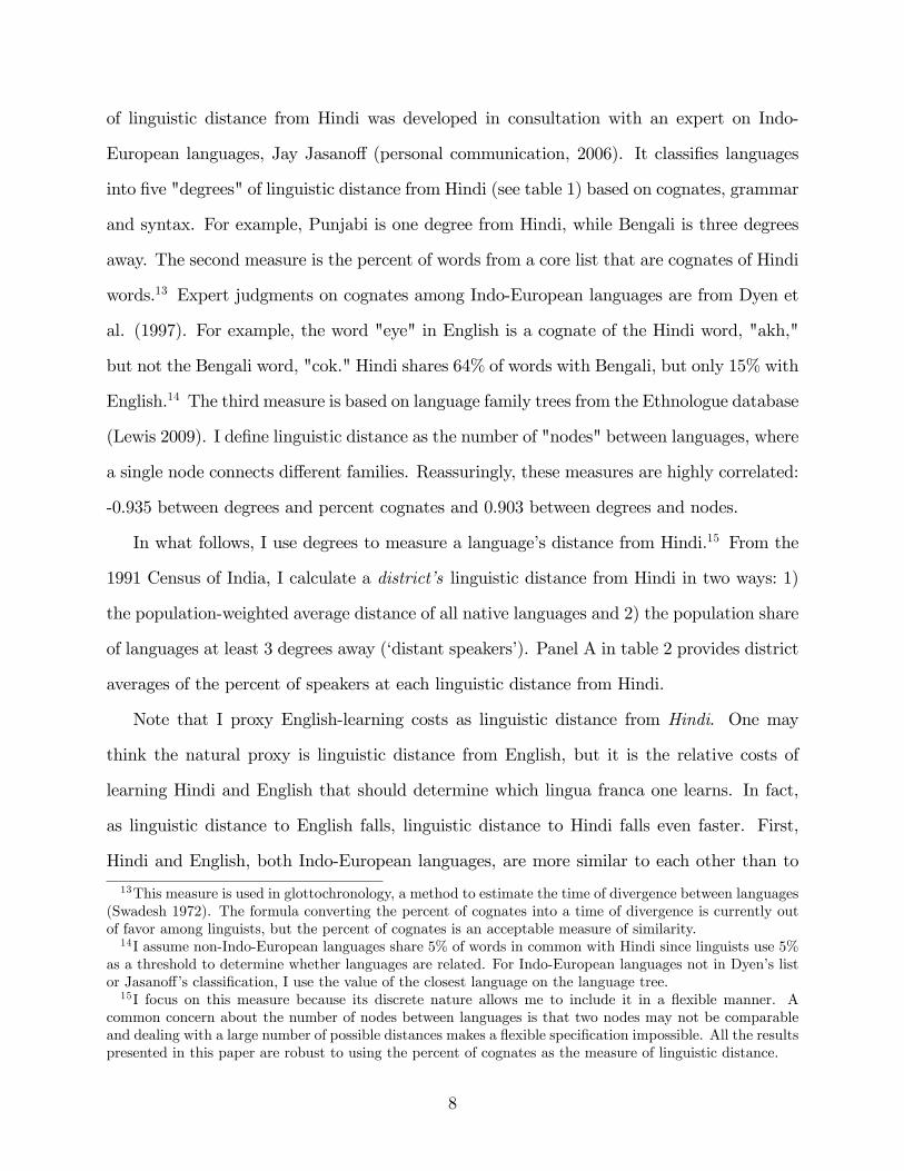
of linguistic distance from Hindi was developed in consultation with an expert on Indo-
European languages, Jay Jasano¤ (personal communication, 2006). It classi�es languages
into �ve "degrees" of linguistic distance from Hindi (see table 1) based on cognates, grammar
and syntax. For example, Punjabi is one degree from Hindi, while Bengali is three degrees
away. The second measure is the percent of words from a core list that are cognates of Hindi
words.13 Expert judgments on cognates among Indo-European languages are from Dyen et
al. (1997). For example, the word "eye" in English is a cognate of the Hindi word, "akh,"
but not the Bengali word, "cok." Hindi shares 64% of words with Bengali, but only 15% with
English.14 The third measure is based on language family trees from the Ethnologue database
(Lewis 2009). I de�ne linguistic distance as the number of "nodes" between languages, where
a single node connects di¤erent families. Reassuringly, these measures are highly correlated:
-0.935 between degrees and percent cognates and 0.903 between degrees and nodes.
In what follows, I use degrees to measure a language�s distance from Hindi.15 From the
1991 Census of India, I calculate a district�s linguistic distance from Hindi in two ways: 1)
the population-weighted average distance of all native languages and 2) the population share
of languages at least 3 degrees away (�distant speakers�). Panel A in table 2 provides district
averages of the percent of speakers at each linguistic distance from Hindi.
Note that I proxy English-learning costs as linguistic distance from Hindi. One may
think the natural proxy is linguistic distance from English, but it is the relative costs of
learning Hindi and English that should determine which lingua franca one learns. In fact,
as linguistic distance to English falls, linguistic distance to Hindi falls even faster. First,
Hindi and English, both Indo-European languages, are more similar to each other than to
13This measure is used in glottochronology, a method to estimate the time of divergence between languages(Swadesh 1972). The formula converting the percent of cognates into a time of divergence is currently outof favor among linguists, but the percent of cognates is an acceptable measure of similarity.14I assume non-Indo-European languages share 5% of words in common with Hindi since linguists use 5%
as a threshold to determine whether languages are related. For Indo-European languages not in Dyen�s listor Jasano¤�s classi�cation, I use the value of the closest language on the language tree.15I focus on this measure because its discrete nature allows me to include it in a �exible manner. A
common concern about the number of nodes between languages is that two nodes may not be comparableand dealing with a large number of possible distances makes a �exible speci�cation impossible. All the resultspresented in this paper are robust to using the percent of cognates as the measure of linguistic distance.
8

non-Indo-European languages spoken in India; there is a strong positive correlation between
linguistic distance from Hindi and from English (0.9714 for percent cognates). At the same
time, languages close to Hindi share on average 66% cognates with Hindi but only 14.6%
cognates with English. To be clear, consider two individuals, one speaks another Indo-
European language close to Hindi and the other speaks a language very far from Hindi. The
�rst individual would �nd both Hindi and English easier to learn than the second individual.
However, the �rst individual will �nd Hindi much easier than English. The second individual
�nds Hindi and English roughly equally di¢ cult. So the �rst individual�s relative cost of
learning English (cost of English - cost of Hindi) is positive, but the second individual�s
relative cost is roughly zero.16 If each person learns one language, the �rst individual should
learn Hindi and the second would be indi¤erent. Assuming a symmetric distribution around
these costs, more people who are like the second individual will learn English and more
people who are like the �rst will learn Hindi.
Also, non-Hindi speakers have historically rebelled against having to learn Hindi, ampli-
fying this tendency. Of course, people can speak more than two languages. Thus, it is an
empirical question whether people who speak languages closer to Hindi (relative to people
who speak languages far from Hindi) are more likely to learn English (it is easier) or less
likely (they only learn Hindi): section 5 demonstrates that the second tendency dominates.
According to this theory, native Hindi speakers should be more likely to learn English
than those far from Hindi. For them, the relative cost of Hindi is irrelevant - they already
speak Hindi - but their cost of learning English is lower than those farther from Hindi (and
thus farther from English). They may not need another lingua franca, however, and could
choose to remain monolingual.
16Using the relative distance (distance from English minus distance from Hindi) would give me similarresults since there is little variation in distance from English. This relative distance is greater for those closeto Hindi than those far from Hindi. I do not focus on this measure because it is only possible for the percentcognates and not the other linguistic distance measures.
9

5 Does linguistic distance predict who learns English?
My identi�cation strategy relies on within-state variation in the relative cost of learn-
ing English driven by linguistic diversity. This strategy rests on two assumptions. First,
linguistic distance from Hindi must predict who learns English and second, it must not be
correlated with omitted factors that a¤ect schooling or exports conditional on state �xed
e¤ects and control variables. In this section, I provide evidence for these two assumptions.
Using data from the Census of India (1961 and 1991), I estimate
Elkt = �0 + �0Dl + �
01Xlk + t + k + �lkt (1)
where Elkt is the percent of native speakers of language l in state k and year t who learn
English, conditional on being multilingual,17 Dl is the distance of language l from Hindi, and
t is a year �xed e¤ect. State �xed e¤ects, k, absorb state heterogeneity. Xlk includes the
share of language l speakers and an indicator for the state�s primary language. I weight by
the number of native speakers and cluster the standard errors by state-language.18
The results con�rm the relationship between learning English and linguistic distance
(table 3). In column 1, I include dummy variables for each linguistic distance. Languages
1 degree from Hindi are the omitted group. Linguistic distance from Hindi signi�cantly
predicts how many multilinguals learn English. The p-value at the bottom of column 1
tests whether the dummy variables are jointly di¤erent from zero. The individual dummy
variables are not strictly increasing, but the deviation is small. Column 2 in table 3 assumes
a linear functional form: One linguistic degree increases the percent of multilinguals who
learn English by 5.8 percentage points. Column 3 includes an indicator for su¢ ciently distant
17The results are similar when I use the number or share of English speakers.18I cluster at this level because I believe the serial correlation will be mostly within local ethnic group:
individuals will be more likely to learn English if their parents and other relatives speak English. The resultsare similar if I cluster by ethnic group (language) or state-language family. There is an argument againstclustering by state because of the state �xed e¤ects and the small number of states in the data (23); however,if I do cluster by state and adjust my critical values accordingly (Cameron, Miller, Gelbach 2007), the resultsare similar (except for one coe¢ cient which is signi�cant only at 10%).
10
speakers: Speaking a language 3 or more degrees from Hindi increases the percent of English
speakers by 29 points relative to speakers of languages 1 and 2 degrees away. Columns 3-7
break these down by year. The relationship between linguistic distance and learning English
existed in 1961, suggesting the relationship is exogenous to recent trade reforms.19
Note that individuals at a linguistic distance of zero (native speakers of Hindi and Urdu20)
who choose to become multilingual tend to learn English. This creates a non-monotonicity
in the relationship between linguistic distance and learning English. The propensity to learn
English dips signi�cantly when we move away from native Hindi speakers and then rises as
we move further. I account for this non-monotonicity in my regressions by controlling for
the percent of native Hindi speakers and calculating the weighted average linguistic distance
only among non Hindi natives. I can also use this non-monotonicity since districts with more
Hindi natives, all else equal, will have more English learners.
The control variables matter as expected: the propensity to learn English is greater in
1991 and increasing in the share of state residents with the same mother tongue (minorities
learn the regional language �rst). I reject the hypothesis that speaking any language other
than Hindi has a uniform e¤ect on learning English by testing the equality of all linguistic
distance �xed e¤ects. Recall the inclusion of state �xed e¤ects: the tendency to learn English
is stronger for people further from Hindi even within a state.
This data allows me to further analyze the relationship between linguistic distance and
language acquisition (results available upon request). Individuals speaking languages further
from Hindi are less likely to learn Hindi, as expected. Reassuringly, linguistic distance to
Hindi does not a¤ect whether someone becomes multilingual.
I next explore how linguistic distance from Hindi predicts whether schools teach English;
I estimate
Mij = �0 + �0Dj + �1Pj + �
02Zj + i + g + �ij (2)
19The coe¢ cient in column 4 is not statistically signi�cant, but I believe this is because of the linearfunctional form. If I include linguistic distance �xed e¤ects (as in column 1), the joint test that the dummyvariables are signi�cantly di¤erent from zero has a p-value very close to 0.20Hindi and Urdu are often considered the same language. Separating them gives similar results.
11

where Mij is English instruction at school level i (primary, upper primary, secondary or
higher secondary) in state j, Dj is the linguistic distance from Hindi of languages spoken
in state j in 1991,21 and Pj is child population (aged 5 - 19, in millions). Zj includes
1987 measures of average household wage income, average income for educated individu-
als, the percent of households with electricity, and the percent of people who: have regular
jobs, have graduated from college, have completed high school, are literate, are Muslim, or
regularly use a train. I include the percent native English speakers, the distance to the
closest of the 10 most populous cities and whether the district is on the coast to account
for trade routes. The vector Zj includes the percent native Hindi speakers to account for
the non-monotonicity described above. To ensure that these results are not driven by native
Hindi populations in the "Hindi Belt" states with high levels of corruption and government
ine¢ ciency, I include an indicator variable for the following states: Bihar, Uttar Pradesh, Ut-
taranchal, Madhya Pradesh, Chhattisgarh, Haryana, Punjab, Rajasthan, Himachal Pradesh,
Jharkhand, Chandigarh and Delhi. In addition, I focus on urban areas and include region22
and grade-level �xed e¤ects (primary, etc.). The data are described in the appendix.
The results show that linguistic distance from Hindi predicts the percent of schools that
teach in English (columns 1-2 of table 4) or teach English as a second language (columns
3-4). An increase in 1 degree in the average linguistic distance from Hindi increases the
fraction of schools teaching in English by 33 percentage points and the fraction teaching
English by 20 points. More Hindi speakers also increases the teaching of English, but only
when using the percent distant speakers measure. Not all estimates are signi�cant, likely
because the data is at the state level, leaving little within-region variation.
21I use a district�s distance from Hindi in 1991 since it is more precise than 1961. The 1961 data lists 1652languages, many of which are di¢ cult to assign a distance from Hindi (in contrast, there are only 114 in1991 due to prior Census classi�cation). Many districts have been divided since 1961, adding further noise.22Data on language instruction in school is at the state level since district-level data is unavailable; thus, I
am unable to include state �xed e¤ects. I also cluster by state and, due to the small number of states (29),adjust my critical values according to Cameron, Miller, Gelbach 2007: the critical values for the 1%, 5% and10% signi�cance levels, drawn from a t-distribution with 27 (= 29 - 2) degrees of freedom, are 2.77, 2.05 and1.70, respectively.
12

5.1 The exclusion restriction
Next, we must consider whether the variation I exploit is correlated with omitted variables
that might bias these results. Most measures of the cost of learning English, e.g. the number
of English speakers, are likely to be correlated with unobserved determinants of schooling
or trade policies. If a local government cares about global opportunities, for example, it
may both promote English and create incentives for FDI. Variation in linguistic distance is
unlikely to be related to export-oriented preferences. When using other measures, we might
also worry about reverse causality: IT �rms can provide English classes. Global opportunities
will not a¤ect a district�s linguistic distance to Hindi. However, we need to verify that there
are no other channels through which linguistic distance might correlate with schooling.
One worry about linguistic diversity is that much of the raw variation is geographic.
Figure 4 maps the raw variation in percent distant speakers: linguistic distance is not ran-
domly distributed. Indo-European languages have traditionally been spoken in the north,
Sino-Tibetan languages in the northeast and Dravidian languages in the south. Since this
geographic variation may be correlated with factors that in�uence schooling or exports, such
as agricultural productivity or culture, I include state (and sometimes district) �xed ef-
fects. I also include district control variables, allowing their e¤ects to di¤er after reforms.
In fact, in the schooling regressions described below, my results are identi�ed o¤ deviations
from pre-existing district trends. In �gure 5 I demonstrate the residual variation that I
use by mapping the residuals from a regression of linguistic distance on state �xed e¤ects
and control variables in vector Zj. This geographically balanced variation is less likely to
be correlated with omitted variables. An important source of this within-state variation is
historical migration. While recent migration is infrequent, people have migrated across India
for millennia, bringing their native languages across present-day boundaries.23
23Some migrants assimilate, but the local diversity shows that these groups retain a separate identity.Linguistic distance to Hindi in 1961 and 1991 are strongly correlated, demonstrating this persistence. On asimilar note, Dravidian languages were traditionally considered native to southern India, but several studieshave provided evidence of Dravidian speakers in western and northwestern regions of the subcontinent prior tothe tenth century CE (Tyler 1968, McAlpin 1981, Southworth 2005). The story of one ethnic group provides
13

One might still worry that communities that speak languages distinct from Hindi di¤er
in ways that might cause bias. Being more forward-looking, for example, could explain the
tendency to learn English and faster growth in education. The results in table 3 provide
evidence against this concern: these groups were more likely to learn English in 1961, before
anyone could anticipate trade liberalization in the 1990s. Similar concerns are that these
communities migrated to faster growing cities before 1991 or had greater preferences for
education. I will rely purely on changes over time when studying enrollment and wages,
accounting for time-invariant heterogeneity.24 Preferences for education, for example, would
only bias my results if they changed di¤erentially after reforms. In section 7, I discuss these
potential threats to validity in detail and provide empirical evidence against these concerns.
6 Impact of linguistic distance from Hindi
The following section discusses three key results. I �rst demonstrate that trade liberal-
ization led to more export opportunities in districts far from Hindi. I then show that growth
in school enrollment grew faster and that returns to education grew slower in these districts
after liberalization. The results suggest that if a district had 2% more English speakers,
the probability it receives any IT �rms increases by 6% points and school enrollment grows
a telling example. In the tenth century CE, the Gaud Saraswat Brahmins (GSBs) were concentrated on thewestern coast of India, in Goa. While there is no direct evidence, GSBs claim to originate from Kashmir. In1351 CE, unrest due to raiding parties sent by a sultan in the Deccan caused some GSB families to migratedown the coast into present-day Karnataka (Conlon 1977). The language still spoken by this group, a dialectof Konkani, is only two degrees from Hindi but the main language in Karnataka is �ve degrees away. Theshare of the population who speak languages exactly two degrees away from Hindi in the rest of Karnatakaaverages 1-4% while in the coastal districts in which the GSBs settled, these languages account for 14-29%of the population. Of course, many others speak languages two degrees from Hindi, but the arrival of thisgroup in 1351 speaks to the persistent e¤ect of historical migration on linguistic diversity today.24At the same time, note that states were created along language lines, that is endogenously created to
maximize within-state linguistic homogeneity. This should lead to very little variation in linguistic distanceto Hindi within a state and exacerbate attenuation bias, which should work against me �nding signi�cantresults. Any remaining omitted variable bias may be ampli�ed if the residual within-state variation inlinguistic distance to Hindi is correlated with time-varying omitted determinants of IT and schooling. Sincehistorical migration is an important source of this variation, it is unlikely that such an omitted variablehad a di¤erential impact after 1991 but not before. For example, a problematic story would be that theGaud Saraswat Brahmins moved to that particular district in present-day Karnataka for a reason that wascorrelated with schooling decisions after 1991 but not before 1991.
14

faster, also by a total of 6-7% points over the 9 year interval from 1993 to 2002.
Note that the spirit of my empirical strategy is that of an instrumental variable: if a
good measure of English learning costs were available, I would use linguistic distance to
Hindi as an instrument. However, a comprehensive district-level measure of this cost is
unavailable, partly because the cost of English is multi-dimensional but more importantly
because the necessary data is unavailable.25 Therefore, I focus on reduced form results using
two measures of linguistic distance: i) the weighted average and ii) percent distant speakers.26
6.1 Information technology
I �rst test whether export opportunities have grown faster in districts with lower costs
of English by studying the IT sector. I estimate
ITjt = �0 + �0Dj + �
01Zj + �
02Wj + t + k + �jt (3)
where ITjt measures IT presence in district j in state k in year t and Dj measures linguistic
distance. Zj is as in equation (2)27 and Wj includes other predictors of IT �rm location28
such as log population, the number of elite engineering colleges,29 the fraction of the district
population that is urbanized, the distance to the closest airport, and the percent of non-
25For example, the measure would include how many schools teach English and how many adults speakEnglish, both unavailable at the district level around 1991.26The most important bene�t of being able to present two stage least squares estimates would have been
in gauging the magnitude of these e¤ects. I present a back-of-the-envelope calculation below to discuss themagnitude of the reduced form results.Also, in section 6.1, I proxy for the cost of learning English with the percent of schools teaching in the
regional mother tongue, the only data available by district. I then instrument for this proxy with measuresof linguistic distance to Hindi. As expected, the results are consistent with the reduced form results.27State �xed e¤ects absorb the state-level controls. The results are robust to excluding vector Zj .28The state �xed e¤ects account for many other predictors of IT �rm location, such as state business
policies. For example, IT �rms may be in�uenced by labor regulation (Besley and Burgess 2004). Thisis unlikely since turnover in IT is remarkably high with �rms raiding each other and employees migratingabroad. Nevertheless, allowing the e¤ect of labor regulation to di¤er over time does not alter my results.29In measuring engineering college presence, I count only the 26 elite engineering colleges, because district-
level data on all engineering colleges are not of the same quality. Another measure is from the list ofaccredited engineering programs from the National Board of Accreditation of the All India Council forTechnical Education. Each program was assigned to a district based on the address of the a¢ liated college.I only include colleges established prior to 1990. Controlling for this measure does not alter my results.
15

migrant engineers in 1987 or 1991. I include year �xed e¤ects and cluster the standard
errors by district. The measures of IT include the existence of any headquarters or branches,
the log number of headquarters and branches and the log number of employees.30 The
state �xed e¤ects ensure that my results are driven by within state variation.31 The data,
described in the appendix, contains �rm-level employment; I assign employees evenly across
branches to estimate employment by district.
Estimating equation (3) reveals a strong positive e¤ect of linguistic distance from Hindi
on IT presence (table 5). In Panel A, I drop the ten most populous cities (as of 1991) since
IT �rms are likely to locate there regardless of English speaking manpower; in Panel B, I
include these cities and an interaction with linguistic distance. The cost of learning English
predicts whether any IT �rm establishes a headquarters or branch in a district. An increase
in 1 degree from Hindi of the average speaker�s mother tongue (three-fourths of a standard
deviation, column 1) results in a 3.7% point increase in the probability of any IT presence
(the dependent variable mean is 15%); a 20% increase in the percent distant speakers (half
a standard deviation, column 2) increases the probability by 6% points. These e¤ects are
economically signi�cant: about a fourth of the e¤ect of housing an elite engineering college.32
Linguistic distance also predicts the number of establishments and employment (columns
3-6). Twenty percent more distant speakers increases the number of establishments by 7-8%
and employment by 40%. A back-of-the-envelope calculation suggests that having 20% more
distant speakers increases the percent of English speakers by 2% and attracts 0.2 more IT
branches (at the mean of 2.5 in 2003) and 240 more employees (at the mean of 600 in 2003).
30I add one before taking the natural log to avoid dropping districts with no IT presence.31I cannot look at changes over time when studying IT because the data does not exist prior to trade
reforms; the assumption that IT was negligible pre-1991 is not unrealistic. In the PROWESS datasetmaintained by the Centre for Monitoring the Indian Economy, only 7 �rms with data in 1990 listed IT astheir economic activity.32Some districts may be unlikely to receive IT for other reasons. While these reasons are orthogonal to
linguistic distance, I con�rm my results by using �rm-level data to focus on districts with any IT between1995 and 2003. I also use the time variation to study whether �rms locate in cities linguistically furtherfrom Hindi earlier or whether they branch out to smaller linguistically distant cities later due to congestion.The results suggest the latter, but there is little variation. Using the age of the oldest �rm as the outcomevariable suggests that IT headquarters were established earlier in areas linguistically further from Hindi, butthe standard errors are large and not always statistically signi�cant (results available upon request).
16
The results in Panel B of table 5, when I include large cities, are nuanced but not
surprising. Being a large city increases IT presence, even after controlling for population.
The positive impact of linguistic distance on the presence of any IT �rm is reduced in large
cities (the interaction term is negative but only marginally signi�cant), but the e¤ect on the
number of establishments is ampli�ed.
It might be that the bene�ts of learning English extend not only to export opportunities
but also to internal trade and integration within the Indian economy which might also have
occurred in the 1990s. The results presented in table 5 are driven primarily by export
opportunities. A conservative estimate is that at least 87% of �rm-years receive non-zero
export revenue. Fifty percent of the �rm-years receive at least 93% of their revenue from
exports and at least 25% of �rm-years do not receive any domestic revenue. Seventy-�ve
percent of �rm-years receive at least 50% of their revenue from exports. Clearly, growth in
the IT �rms in this sample was driven by export opportunities. However, it is still possible
that other manufacturing or other services involved in intra-India trade may have grown
di¤erentially in these districts contributing to changes in school enrollment rates and skilled
wage premiums. I use two di¤erent datasets to examine this further. Neither dataset provides
su¢ cient data to be conclusive, but together they provide support for the claim that these
districts did not experience di¤erential growth in non-export sectors.
Using the industrial classi�cations available in the National Sample Survey data, I do
not �nd evidence of di¤erential employment growth in linguistically distant districts in the
following industries: �nancial services, hotels and restaurants, agriculture, transportation,
and other services. There is some evidence of di¤erentially hampered employment growth in
manufacturing and communications but improved employment growth in wholesale, retail
and repair but these results are not particularly robust (results available upon request). Using
a �rm-level panel dataset maintained by the Centre for Monitoring the Indian Economy,
PROWESS, I �nd no evidence that districts linguistically further from Hindi experienced
greater growth in domestic (not export) revenue. The standard errors are large, making it
17

di¢ cult to conclude that there is no di¤erence in domestic income growth for these districts,
but the coe¢ cients are often negative suggesting that if anything, these districts produced
less for domestic trade (results available upon request).
6.2 Education
To study how schooling responds in districts with di¤erent costs of learning English, I
use enrollment from three years (1987, 1993, and 2002) to estimate
log (Sijt)� log(Sijt�1) = �0 + �0Dj � I (t = 2002) + �1 log (Sijt�1) + �02Pjt (4)
+�03Zj � I (t = 2002) + �4Bjt + i + j + gt + �ijt
where Sijt is enrollment in grade i in district j, region g and time t, I (�) is an indicator
function, Dj and Zj are as above33 and Pjt includes log child population and the fraction
urban at time t and t� 1. i is a grade �xed e¤ect. I use only data from urban areas34 and
cluster by district. I also include a proxy for skilled labor demand growth, Bjt, to control
for other changes in demand for education. Calculated along the lines of Bartik (1991), Bjt
is an average of national industry employment growth rates weighted by pre-liberalization
industrial composition of district employment. Bjt should not be correlated with local labor
supply shocks but may pick up some of the e¤ect of reforms through national employment
growth. Since the data consist of the number of students enrolled, not enrollment rates,
I control for population aged 5-19 from the 1991 and 2001 Census.35 Details are in the
appendix. Enrollment increased dramatically, by 32%, between 1993 and 2002.
33Since I already include district �xed e¤ects, Zj is interacted with I (t = 2002), allowing pre-liberalizationdi¤erences to have a di¤erent e¤ect post reform. The results are robust to excluding these controls.34The results are robust to using total school enrollment in the district; rural areas show no signi�cant
di¤erences in enrollment (see section 7.1). I also consider whether initial urbanization was correlated withlinguistic distance or whether linguistically distant districts become more urbanized over time in section 7.35I cannot use a more precise age group since children start school at di¤erent ages and are often held
back. Since enrollment and population are in logs, using the ratio of enrollment to child population gives meidentical point estimates and almost identical standard errors. Using child population measures from 1993and 2002 does not impact the results, but the age ranges reported di¤er between these years.
18

Three years of data gives me one period of growth before liberalization and one after:
I can therefore exploit the variation across time by including district �xed e¤ects. In a
growth regression such as equation (4), these �xed e¤ects control for district-speci�c trends.
This speci�cation already eliminates bias from potentially omitted variables at the district
level, but I make it even more rigorous by allowing for region-speci�c changes in trend, by
including region �xed e¤ects interacted with time.36
I �nd that educational attainment rises more in districts with lower costs of learning
English (table 6). Panel A uses the weighted average while panel B uses the percent distant
speakers measure of linguistic distance. Columns 1-2 pool all grades; columns 3-8 stratify
the sample by grade. Both measures of linguistic distance predict an increase in enrollment
growth. One degree in average linguistic distance to Hindi would increase overall growth
by 7% over the 9 year period; an increase of 20% distant language speakers would increase
enrollment growth by 6%. At the primary and upper primary levels, the coe¢ cients for girls
are larger than for boys, but the di¤erence is not statistically signi�cant. Panels C and D
replicate panels A and B but control for statewide breaks in enrollment trends. Some of the
results are robust to identifying o¤ deviations to statewide changes in trend, but many of
the coe¢ cients are no longer statistically signi�cant.
The magnitudes are large, but not unrealistic. For the average district, they imply that
a district with 2% more English speakers would see urban school enrollment grow by 1800-
3600 additional students in primary school, 1800-2700 in upper primary and 1500-3000 in
secondary school. Recall that from 1993 to 2002, enrollment on average grew by 13000 (21%)
in primary school, 9000 (30%) in upper primary and 15000 (60%) in secondary.
As noted above, school enrollment is likely responding to global, English-intensive op-
portunities besides IT, making it tricky to compare the impact on IT growth and school
enrollment. There were approximately 800,000 employees in IT in 2003; at the prevailing
36Recall that regions are larger than states which are larger than districts. In a robustness check, I alsotake out state-speci�c changes in trend but these eliminate much of the variation available in the district-leveldata. In addition, the signal to noise ratio falls, exacerbating the attenuation bias.
19

20% annual growth rate, we would expect 160,000 new IT jobs the following year or about
420 new jobs per district. A district with 20% more distant speakers would receive 40% more
jobs (column 5 in table 5) or 180 more new jobs. This district would also have 400 more
secondary school students per grade. Not all of them would be looking for an IT job after
graduation and individuals from other sectors might choose to move into IT, but compar-
ing these two numbers gives us a rough estimate of the importance of IT relative to other
English-intensive jobs: IT jobs can explain about 45% of the increase in school enrollment.
We may also want to explore growth in districts with more Hindi speakers, since Hindi
speakers are more likely to learn English than individuals 1 or 2 degrees away. Districts with
more native Hindi speakers exhibit larger increases in enrollment growth; the e¤ect is similar
in magnitude to that of distant speakers. As in table 3, the e¤ect of Hindi speakers is more
pronounced when linguistic distance is measured as percent distant speakers. This result is
reassuring since it con�rms that places with more English speakers saw a bigger increase in
school enrollment growth using slightly di¤erent variation.
There are two avenues through which new job opportunities could increase schooling.
I focus on human capital responses to returns to education. Another channel is through
increased family income: it is unlikely that this channel drives all of my results since the new
job opportunities were concentrated among young adults. This should have a larger e¤ect
in lower grades while the results indicate similar, if not bigger, e¤ects at older ages.
6.2.1 School enrollment by language of instruction
These results demonstrate that school enrollment responded, but the data does not sep-
arate enrollment by language of instruction. I could instead use new data on enrollment by
media of instruction from the District Information System for Education (see appendix), but
this data is only available after 2002. Not being able to control for pre-liberalization enroll-
ment by language is a problem because I cannot distinguish between pre-existing di¤erences
between districts and the impact of growth in export-related jobs.
20

Nevertheless, I compare enrollment in English to enrollment in Hindi and other local
languages and account for unobserved heterogeneity using district �xed e¤ects. I estimate:
Eljt = �0 + �0Dj � l + �1Pjt + �02Zjl (5)
+ l + j + kt + �ijt
where Eljt is the fraction of children enrolled in grades 1-8 in language l 2 {English, Hindi,
and others grouped together}37 in district j, state k and time t, Pjt is child population, Dj � lis linguistic distance interacted with an indicator for English instruction, and Zjl is a vector
of control variables, interacted with language �xed e¤ects.38 I also include �xed e¤ects for
language and state-year. As before, I include all interactions with percent of Hindi speakers
to account for the non-monotonicity. Standard errors are clustered by district.
The results are presented in table 7. The �rst two columns pool together all years, while
columns 3-4 allow the e¤ect to vary by year. An increase in one degree in average linguistic
distance to Hindi (column 1) increases school enrollment in English by 8.4 percentage points
relative to enrollment in Hindi and other languages. An increase in distant language speakers
of 20 percentage points (column 20) increases enrollment in English by 6.8 percentage points.
Columns 3-4 allow trends in enrollment to di¤er by linguistic distance. English enroll-
ment in 2002 was already signi�cantly more responsive to linguistic distance than enrollment
in Hindi and other languages, but the interactions with the year dummies are also all sta-
tistically signi�cant and more or less increasing in magnitude. These results demonstrate
that English enrollment in linguistically distant districts grew faster than enrollment in other
languages between 2002 and 2007.
37Due to data limitations, I have to group together enrollment in all other languages.38Zjl only includes interactions with whether a district is in the Hindi Belt, the percent of native English
speakers and the percent of native Hindi/Urdu speakers, but the results are robust to including interactionswith demographic characteristics of the district used in speci�cation (4).
21

6.3 Returns to education
Having demonstrated that districts with greater linguistic distance to Hindi experienced
greater IT and school enrollment growth after trade liberalization, I now turn to the general
equilibrium implications for skilled wage premiums. The theoretical prediction is ambiguous
and depends on the relative magnitudes of the demand shocks. I study how the impact of
globalization on returns to education varies with linguistic distance by estimating
log (wagen) = �0 + �01Dj � I (t = 1999) + �02Dj � I (t = 1999) �HSn + �03Dj � I (t = 1999) � Cn
+�01Dj �HSn + �02Dj � Cn + �3I (t = 1999) �HSn + �4I (t = 1999) � Cn
+�5HSn + �6Cn + �07Yn + �
08Wj � I (t = 1999) + j + t + kt + �n (6)
where wagen is weekly wage earnings of individual n in district j in year t 2 f1987; 1999g,
HSn and Cn are indicators for high school and college completion, respectively and Yn and
Wj contain individual and district characteristics. I only include nonzero wage earners. Yn
includes age, age squared, gender, marital and migration status. At the district level, Wj
includes the percent of native English speakers, the distance to the closest big city, whether
the district is coastal and predicted labor demand. To account for the non-monotonicity in
linguistic distance, I include the percent of native Hindi speakers interacted with I (t = 1999),
HSn, Cn and all triple interactions. I have two years of data, allowing me to include district
�xed e¤ects, controlling for district wages. As in equation (4), I also include state �xed
e¤ects interacted with time which control for state trends. I also cluster the standard errors
by district and weight the observations.39
Skilled wage premiums rose by less in districts with lower English costs from 1987 to 1999,
particularly for high school graduates (see table 8). The coe¢ cients �2 and �3 are always
negative, but not always signi�cant. The magnitudes are economically signi�cant. The wage
premium for high school graduates rises by 5% less over 12 years per degree of linguistic
39The results are robust to including the district vector of controls, Zj , interacted with I (t = 1999), butI do not include these in the main speci�cation since the controls are from 1987, the �rst year of this data.
22

distance, relative to a premium of 54% for high school graduates in 1987. Stratifying the
sample by age and gender reveals that the results are driven by men and older workers.
Note that we should be cautious in interpreting these results. First, since the data do
not distinguish between instruction in di¤erent languages, I focus on average returns to
education. Second, the wage data from the National Sample Surveys is the best available
data over this time period, but is not particularly suited for this study since the sample
a¤ected by export-related jobs is quite small. Researchers are also skeptical of this wage
data since it is self-reported and not veri�able; many individuals work in the informal sector.
Nevertheless, this provides suggestive evidence that the supply side response of human capital
may mitigate rising skilled wage premiums.
7 Threats to validity and robustness checks
This section provides evidence against various threats to validity and some robustness
checks. I omit most tables, but all results are available upon request. First, I consider
whether di¤erences in preferences for education between communities that speak di¤erent
languages could explain the results. I con�rm that linguistic distance is not correlated with
the supply of schools by estimating a regression of the log number of schools in a district in
1993 on linguistic distance to Hindi, child population, state �xed e¤ects and district control
variables. Linguistic distance also does not predict the number of schools o¤ering courses in
speci�c �elds, such as science, in 1993.
Another way to test preferences for education is to look at pre-trends in school enrollment.
I run the following regression, similar to equation (4), using data from 1987 and 1993:40
log (Sij1993)� log(Sij1987) = �0 + �0Dj + �1 log (Sij1987) + �
02Pj (7)
+�03Zj + �4Bj + i + g + �ij
40Data from 1991, when reforms were announced, would be preferable but is not available. Nevertheless,many reforms were implemented only after 1993 and enrollment is unlikely to have responded so quickly.
23

The di¤erences speci�cation accounts for time-invariant heterogeneity across districts and
the region or state �xed e¤ects account for di¤erential trends.
Results, broken down by grade and gender, are presented in table 9. Linguistic distance
is not correlated with pre-trends in school enrollment. Often the coe¢ cient is even negative,
although almost always insigni�cant. The only coe¢ cient signi�cant at 5% is for secondary
school boys and is negative. This might cause concern if low enrollment in 1993 allowed for
more improvement in the subsequent period, but my estimates control for this trend and
allow for convergence by controlling for pre-enrollment.
Another concern is that these communities may have di¤erent propensities to migrate.
Large movements of people may alter the languages spoken in an area, but migration in
India is quite infrequent. According to the 1987 National Sample Survey, only 12.3% of
individuals in urban areas had moved in the past �ve years, only 6.8% had moved from a
di¤erent district and only 2.4% had moved across states. These numbers were even smaller
in 1999. I calculate linguistic distance from Hindi in 1991 which avoids bias from endogenous
migration after reforms. In addition, random migration across states before reforms will not
bias my coe¢ cients: it will simply bring linguistic distance measures closer to the mean for
India. It would only be problematic if migrants had greater preferences for education and
speakers of distant languages di¤erentially moved prior to 1991 into districts that will receive
export-oriented growth. Given how infrequently people move and the size of these districts,
it is unlikely this a¤ected my measure of linguistic diversity. The strong correlation between
linguistic distance to Hindi in 1961 and 1991 (0.81 for the weighted average and 0.88 for
percent distant speakers) con�rms that the variation is not due to recent migration. Using
the National Sample Survey, I �nd that migrants tend to be more educated, but linguistic
distance is usually not correlated with the likelihood of having migrated, except for some
evidence of fewer recent migrants in districts with higher weighted average linguistic distance.
Finally, I consider the concern that districts that are linguistically distant from Hindi
are less integrated within India since they do not speak the native o¢ cial language. This
24

may have impacted the evolution of industries or interstate trade. Conditional on district
controls and state �xed e¤ects, linguistic distance is not correlated with the percent of workers
employed in speci�c industries, such as manufacturing, tourism or �nance before 1987.41 A
related concern is that districts linguistically distant from Hindi might have been initially
more urbanized attracting IT �rms or that these districts urbanized faster. Using census
data on rural and urban populations, I �nd that these districts were not more urbanized in
1991 and that they did not urbanize faster from 1991 to 2001.
7.1 Robustness checks
Finally, I discuss a few robustness checks in detail. First, I estimate a two stage least
squares model using a proxy for the cost of learning English and instrument with linguistic
distance. The proxy is the percent of schools that teach in the regional mother tongue (the
only information available by district). Since English is not a regional mother tongue, this
proxy is a lower bound on schools not teaching in English. The instruments are the share of
residents who speak languages at each degree of linguistic distance from Hindi.
The results from this 2SLS estimation are consistent with the reduced form, although
the standard errors are quite large. The contribution of this exercise is to provide a sense of
the magnitudes of these e¤ects. If 10% more schools taught in the mother tongue (slightly
less than half a standard deviation), a district would be 10% points less likely to have any
IT presence, the number of branches would fall by 10% and employment by 50%. The41Clingingsmith (2008) demonstrates that growth in manufacturing in the 1930s led to declines in linguistic
heterogeneity as minorities learned other languages and claimed new mother tongues. I do not believe thisinvalidates my strategy. First, despite all the industrial development before 1991, Indian districts stillexhibit tremendous linguistic heterogeneity, much of which is geographic. Identity is strongly associatedwith mother tongue; people may learn other languages, but in the time frame I study, will not claim anew mother tongue. Second, my source of variation is a speci�c type of linguistic diversity, not simplyheterogeneity. Third, the potentially problematic biases are unlikely. This phenomenon would be a concernonly if linguistic heterogeneity fell at di¤erent rates in di¤erent types of districts within a region and peopleof minority languages have di¤erent preferences for education. This seems unlikely. There are also extremelyfew native English speakers (0.02%); we need not worry that many highly able minorities chose to call Englishtheir native language. Nevertheless I control for percent native English speakers. If linguistic heterogeneityfell in districts that had more manufacturing in the 1930s, this could possibly a¤ect linguistic distance toHindi. However, it is most likely people switched to Hindi or to the regional language; neither move willa¤ect my measures since I control for Hindi speakers and focus on within region variation.
25

magnitudes for school enrollment growth are also economically signi�cant: a 10% increase
in how many schools teach in the mother tongue reduces enrollment growth by 12% over 9
years. Returns to education rise by 2-5% points more over 12 years.
The second robustness check is to use historical variation in the share of English speakers
in each district as an alternate source of variation in English prevalence from the 1961
census.42 While the share of English speakers today is endogenous - likely correlated with
unobservable determinants of education and IT growth - the historical share of speakers is
less likely to be biased: we need not worry about reverse causality, for example. However,
given the history of education in India - most education was in English during British rule
- historical English literacy may be correlated with other historical factors that have lasting
e¤ects. While this variation is not necessarily better, it is likely to be correlated with di¤erent
omitted variables than linguistic distance to Hindi.
The results are similar to those found using linguistic distance to Hindi. A 10% increase
in the share of English bilinguals (40% of a standard deviation) increases the probability of
any IT presence by 14-17% points and the number of branches and employment by 2-3% and
5-9% respectively. A 10% increase in the share of English speakers in 1961 would increase
enrollment growth by 0.7-2.5%.43 Returns to education are not statistically signi�cant.
My last robustness check focuses on rural areas of the districts that experienced urban
growth in high-skilled exporting opportunities. It is not obvious what we would expect.
Since these rural areas are closer to the exporting urban areas, we might see more rural-
urban migration in linguistically distant districts. If motivated families migrated with young
children, we would see a negative e¤ect on schooling in rural areas. If, instead, young people
migrated after completing their schooling in rural areas, we may see positive spillovers. The
results demonstrate that changes in rural enrollment trends after 1993 are not correlated
42We have this data only by state in 1991; district data in 1961 only covers the 6 most common languages.43As above, these results are statistically signi�cant when accounting for region-speci�c trends, but not
state-speci�c trends. Similarly, the IT results are strongly statistically signi�cant when including region �xede¤ects, but not with state �xed e¤ects. This is not surprising given that there were fewer states in 1961 andthe census only published second language data on people who spoke the 6 most common languages in thedistrict. This source of measurement error would bias the coe¢ cients towards zero.
26

with linguistic distance to Hindi.
This exercise also constitutes a further check on my exclusion restriction. Many alternate
explanations for why school enrollment grew faster in urban areas of linguistically distant
districts after 1993 should be relevant for rural areas as well. For example, if preferences for
education are correlated with linguistic distance to Hindi, causing faster growth in certain
districts, we would expect enrollment trends to di¤er also in rural areas. The lack of evidence
for di¤erential changes in rural areas supports my identi�cation strategy.44
8 Conclusion
In this paper, I demonstrated how districts with di¤ering abilities to take advantage of
global opportunities responded to the common shock of globalization. I exploited exogenous
variation in the cost of learning English, a skill that is particularly relevant for export-related
jobs. I �rst showed that linguistic distance from Hindi predicts whether individuals learn
English. Next, I showed that IT �rms were more likely to set up in districts further from
Hindi. Finally, I demonstrated that these districts experienced greater increases in school
enrollment growth, but smaller growth in the skilled wage premium.
This paper distinguishes two types of human capital investment: learning a second lan-
guage and attending an additional year of school. While most research on human capital
focuses on schooling, an understanding of human capital acquisition in linguistically frag-
mented countries requires that we think about both types. In practice, they are likely to
be correlated but not perfectly: individuals often learn second languages in school, but they
are only likely to gain �uency if instruction is in that second language. This paper shows
that some districts were better prepared to take advantage of global opportunities because
there was greater investment in English human capital (for exogenous reasons), despite no
signi�cant di¤erences in general schooling human capital.
44This assumes languages are spread evenly across rural and urban areas, which may not be true; unfor-tunately, the data needed to con�rm this is not available.
27
There are two important implications. The �rst relates to how countries can mitigate
adverse e¤ects of globalization on inequality. During trade liberalization, governments should
consider policies to help individuals acquire the skills necessary for global opportunities.
While the source of variation used in this paper is speci�c to the Indian case, and the skill
- English literacy - is especially relevant in the Indian example, the result that the adverse
impacts of trade liberalization can be mitigated is not unique to India. In particular, investing
in the accessibility and quality of schools and institutions that help low-skilled workers retrain
could mitigate the rise in the skilled wage premium and the resulting inequality when other
countries open up to trade.45 The second implication is the evidence for a long run e¤ect of
globalization: factor supply may mitigate the increase in wage inequality over time.
Trade liberalization may also have impacted other development indicators, such as fer-
tility. IT �rms employ more women than traditional Indian �rms. The male-female ratio
among workers was 80:20 in 1987, but 77:23 in software �rms and 35:65 in business process-
ing �rms (NASSCOM 2004). Anecdotal evidence suggests that women work in call centers
between school and getting married, potentially impacting age of �rst marriage and fertility
rates. The impact on these other outcomes is an important avenue for future research.
9 References
Arora, A. and A. Gambardella (2004). "The Globalization of the Software Industry: Perspec-tives and Opportunities for Developed and Developing Countries." NBER Working Paper 10538,National Bureau of Economic Research, Cambridge, MA.
Arora, A. and S. Bagde (2007). "Private investment in human capital and Industrial development:The case of the Indian software industry" (mimeo) Carnegie Mellon University.
Attanasio, O., P. Goldberg and N. Pavcnik (2004). �Trade Reforms and Wage Inequality in Colom-bia,�Journal of Development Economics 74, 331-366.
Attanasio, O. and M. Szekely (2000). �Household Saving in East Asia and Latin America: In-equality Demographics and All That�, in B. Pleskovic and N. Stern (eds.), Annual World BankConference on Development Economics 2000. Washington, DC: World Bank.
45This need not be limited to developing countries either. Job training programs in the US are potentiallyone way to reduce the impact of trade on low-skilled workers.
28

Azam, M., A. Chin, and N. Prakash (2010). "The Returns to English-Language Skills in India,"(mimeo) University of Houston.
Bartik, T. (1991). Who Bene�ts from State and Local Economic Development Policies? Kalamazoo:W.E. Upjohn Institute for Employment Research.
Besley, T. and R. Burgess (2004). "Can Labor Regulation Hinder Economic Performance? Evidencefrom India," The Quarterly Journal of Economics 119(1), 91-134.
"Busy signals: Too many chiefs, not enough Indians," The Economist, September 8, 2005.
�Can India Fly? A Special Report,�The Economist, June 3-9, 2006.
Clingingsmith, D. (2008). "Bilingualism, Language Shift and Economic Development in India,1931-1961." (mimeo) Case Western Reserve University.
Conlon, F. (1977). A Caste in a Changing World. Berkeley, CA: University of California Press.
Cragg, M.I. and M. Epelbaum (1996). �Why HasWage Dispersion Grown in Mexico? Is It Incidenceof Reforms or Growing Demand for Skills?�Journal of Development Economics 51, 99-116.
Dyen, I., J. Kruskal and P. Black (1997). FILE IE-DATA1. Available at http://www.ntu. edu.au/education/langs/ielex/HEADPAGE.html.
Edmonds, E., N. Pavcnik and P. Topalova (2007). "Trade Adjustment and Human Capital Invest-ments: Evidence from Indian Tari¤ Reform." NBER Working Paper No. 12884, National Bureauof Economic Research, Cambridge, MA.
Feenstra, R.C. and G. Hanson (1996). �Foreign Investment, Outsourcing and Relative Wages.�In R.C. Feenstra, G.M. Grossman and D.A. Irwin, eds., The Political Economy of Trade Policy:Papers in Honor of Jagdish Bhagwati, MIT Press, 89-127.
Feenstra, R.C. and G. Hanson (1997). �Foreign Direct Investment and Relative Wages: Evidencefrom Mexico�s Maquiladoras.�Journal of International Economics, 42(3), 371-393.
Feliciano, Z. (1993). �Workers and Trade Liberalization: The Impact of Trade Reforms in Mexicoon Wages and Employment.�(mimeo) Harvard University.
Goldberg, P. and N. Pavcnik (2004). �Trade, Inequality, and Poverty:What DoWe Know? Evidencefrom Recent Trade Liberalization Episodes in Developing Countries,� Brookings Trade Forum,Washington, DC: Brookings Institution Press: 223�269.
Hanson, G. and A. Harrison (1999). �Trade, Technology and Wage Inequality in Mexico.�Industrialand Labor Relations Review 52(2), 271-288.
Hohenthal, A. (2003). "English in India; Loyalty and Attitudes," Language in India, 3, May 5.
Jasano¤, J. (2006). Diebold Professor of Indo-European Linguistics and Philology, Harvard Uni-versity. Personal communication.
29

Jensen, R. (2011). Economic Opportunities and Gender Di¤erences in Human Capital: Experimen-tal Evidence for India. (mimeo) University of California-Los Angeles.
Kamat, A. (1985). Education and Social Change in India. Bombay: Somaiya Publications.
Karnik, K., ed. (2002). Indian IT Software and Services Directory 2002. National Association ofSoftware and Service Companies, New Delhi.
Kremer, M. and E. Maskin (2006). �Globalization and Inequality.�(mimeo) Harvard University.
Ku, H. and A. Zussman (2010). "Lingua franca: The role of English in international trade." Journalof Economic Behavior & Organization 75, 250-260.
Levinsohn, J. (2004). "Globalization and the Returns to Speaking English in South Africa." NBERWorking Paper 10985. National Bureau of Economic Research, Cambridge, MA.
Lindert, P. and J. Williamson (2001). �Does Globalization Make the World More Unequal?�NBERWorking Paper No. 8228, National Bureau of Economic Research, Cambridge, MA.
Lewis, M. Paul (ed.), 2009. Ethnologue: Languages of the World, Sixteenth edition. Dallas, Tex.:SIL International. Online version: http://www.ethnologue.com/.
McAlpin, D. (1981). Proto-Elamo-Dravidian: The Evidence and its Implications, Philadelphia, PA:The American Philosophical Society.
Mehta, D., ed. (1995). Indian Software Directory 1995-1996. New Delhi: National Association ofSoftware and Service Companies.
Mehta, D., ed. (1998). Indian Software Directory 1998. New Delhi: National Association ofSoftware and Service Companies.
Mehta, D., ed. (1999). Indian IT Software and Services Directory 1999-2000. New Delhi: NationalAssociation of Software and Service Companies.
Munshi, K. and M. Rosenzweig (2006). "Traditional Institutions Meet the Modern World: Caste,Gender, and Schooling Choice in a Globalizing Economy," American Economic Review 96(4), 1225-1252.
Nanda, R. and T. Khanna (2010). "Diasporas and Domestic Entrepreneurs: Evidence from theIndian Software Industry." Journal of Economics and Management Strategy (forthcoming).
NASSCOM, 2004. Strategic Review 2004. New Delhi: National Association of Software and ServiceCompanies, 185-194.
Nurullah, S. and J. Naik, 1949. A Student�s History of Education in India, 1800-1947. Bombay:Macmillan and Company Limited.
Oster, E. and M. B. Millett (2010). "Do Call Centers Promote School Enrollment? Evidence fromIndia." (mimeo) University of Chicago.
30

Panagariya, A. (2004). "India�s Trade Reform: Progress, Impact and Future Strategy" Interna-tional Trade 0403004, EconWPA.
Robbins, D. (1995a). �Earnings Dispersion in Chile after Trade Liberalization.�Harvard Institutefor International Development, Cambridge, MA.
Robbins, D. (1995b). �Trade, Trade Liberalization, and Inequality in Latin America and East Asia:Synthesis of Seven Country Studies.�Harvard Institute for International Development, Cambridge,MA.
Robbins, D. (1996a). �Stolper-Samuelson (Lost) in the Tropics: Trade Liberalization and Wagesin Colombia 1976�94.�Harvard Institute for International Development, Cambridge, MA.
Robbins, D. (1996b). �HOS Hits Facts: Facts Win. Evidence on Trade andWages in the DevelopingWorld.�Harvard Institute for International Development, Cambridge, MA.
Robbins, D. and T. Gindling (1997). �Educational Expansion, Trade Liberalisation, and Distribu-tion in Costa Rica.� In Albert Berry, ed., Poverty, Economic Reform and Income Distribution inLatin America. Boulder, Colo.: Lynne Rienner Publishers.
Robbins, D., M. Gonzales, and A. Menendez (1995). �Wage Dispersion in Argentina, 1976�93:Trade Liberalization amidst In�ation, Stabilization, and Overvaluation.�Harvard Institute for In-ternational Development, Cambridge, MA.
Sanchez-Paramo, C. and N. Schady (2003): �O¤ and Running? Technology, Trade, and the Ris-ing Demand for Skilled Workers in Latin America,�World Bank Policy Research Working Paper3015.Washington, DC: World Bank.
Southworth, F. (2005). Linguistic Archaeology of South Asia. New York: RoutledgeCurzon.
Swadesh, M. (1972). "What is glottochronology?" In M. Swadesh, The origin and diversi�cationof languages. London: Routledge & Kegan Paul: 281-284.
Topalova, P. (2004). "Trade Liberalization and Firm Productivity: The Case of India." IMFWorking Paper 04/28, International Monetary Fund.
Topalova, P. (2005). "Trade Liberalization, Poverty, and Inequality: Evidence from Indian Dis-tricts." NBER Working Paper 11614, National Bureau of Economic Research, Cambridge, MA.
Tyler, S. (1968). "Dravidian and Uralian: The lexical evidence," Language 44, 798-812.
Wei, S. and Y. Wu (2001). �Globalization and Inequality: Evidence from Within China.�NBERWorking Paper 8611, National Bureau of Economic Research, Cambridge, MA.
Wood, A. (1997). �Openness and Wage Inequality in Developing Countries: The Latin AmericanChallenge to East Asian Conventional Wisdom.�World Bank Economic Review 11(1), 33-57.
31

10 Data Appendix
10.1 Information technologyI collected and coded data on IT �rms from the National Association of Software and Service
Companies (NASSCOM) directories published in 1995, 1998, 1999, 2002 and 2003. These directoriescontain self-reported �rm level data on the location of �rm headquarters and branches, and thenumber of employees. According to NASSCOM, the sample accounts for 95% of industry revenuein most years (Mehta 1995, 1998, 1999; Karnik 2002). While the data is self-reported, �rms have noreason to under-report their performance since IT �rms receive generous tax exemptions. Summarystatistics are presented in table A1.
10.2 Enrollment and language of instruction in 1993, 2002Data on school enrollment comes from the Sixth and Seventh All India Educational Surveys
(SAIES), conducted by the National Council of Educational Research and Training, which beganin September 1993 and September 2002 respectively. The surveys collect school level data onenrollment, facilities, languages taught, courses available, teacher quali�cations and other aspectsof education. The only data currently available from the 2002 data is enrollment, by grade andgender. Some data from 1993, such as languages taught, are only available at the state level. Alldata is separated into urban and rural setting. Summary statistics are presented in table A2.
10.3 Enrollment by language of instruction in 2002-2007Beginning in 2002, the Indian government began compiling data on school enrollment by lan-
guage of instruction as part of a broader e¤ort to collect administrative school-level data (DistrictInformation System for Education, DISE). Using school-level surveys among primary and upper pri-mary schools, each district collected data on enrollment in various categories (grade, gender, caste,etc.) and characteristics of the schools, such as the number of teachers, and teacher quali�cations.Enrollment is available for the most common languages in each district and then other languagesgrouped together. I group Hindi and Urdu together and group all other languages together. I usedata on child population and the number enrolled by language of instruction, aggregated to thedistrict level. The data is available for 2002 and then annually from 2004 to 2007.
10.4 Employment, enrollment in 1987 and district-level controlsData on employment and returns to education are from the National Sample Surveys (NSS)
conducted in 1987-1988 and 1999-2000.46 The NSS provides individual-level information on wagespaid in cash and in-kind as well as employment status, industry and occupation codes and obser-vation weights. Employment status includes working in household enterprises (self-employed), asa helper in such an enterprise, as a regular salaried/wage employee and as casual day labor. Inaddition, the data conveys whether individuals are seeking work, attending school or attendingto domestic duties. I examine employment in agriculture, manufacturing, wholesale/retail/repair,hotel & restaurant services, transport services, communications (post and courier), �nancial inter-mediate/insurance/real estate and other services (education, health care, civil).
46NSS surveys were conducted in 1983-1984 and 1993-1994, but district identi�ers are not available.
32
This data was also used to calculate 1987 school enrollment and district-level controls.47 Iconstruct district-level measures of grade school enrollment at the primary, upper primary andsecondary levels. The NSS also contains household-level information on household structure, de-mographics, employment, education, expenditures, migration and assets, from which I calculatedistrict averages of all control variables mentioned above such as household wage income, the per-cent of working-age adults who are engineers, the percent Muslim, the percent who regularly travelby train and the percent of households that have electricity.
10.4.1 Predicted labor demand growth
Using this NSS data and following Bartik (1991), I calculate the proxy for the growth in labordemand for educated workers using the formula
b"Eit = 54Xj=1
eeE�i;j;1983ee�i;j;1983!�
ei;j;1983ei;1983
��ee�i;j;t � ee�i;j;t�1ee�i;j;t�1�
where b"Eit is the predicted skilled labor demand growth from year t � 1 to t in industry j for areai, e denotes employment and ee�i denotes employment outside area i. The superscript E indicatesworkers with at least a high school degree. Speci�cally, ee�i;j;t is national employment outside areai in industry j in year t, eeE�i;j;t is national employment outside area i in industry j for educatedworkers, and ei;j;t is employment in area i in industry j. NSS data for 1983 does not contain districtidenti�ers so I use a larger aggregation of multiple districts that is smaller than a state. I match54 2-digit categories from the National Industrial Classi�cation of 1970, 1987 and 1998.
Thus, the proxy is a weighted average of growth rates of national industry employment wherethe weights are the 1983 share of multi-district employment in each industry. To predict labordemand for educated workers in particular, I further weight these growth rates using the share ofemployment with at least a high school education.
10.4.2 Other controls
Using latitude and longitude data, I calculate the distance from each district to the closestof the 10 biggest cities in India and to the closest airport operated by the Airports Authority ofIndia. As a measure of elite engineering college presence I count the number of Indian Institutes ofTechnology and Regional Engineering Colleges (now called the National Institutes of InformationTechnology) in each district. All of them were established prior to 1990, although some were notgiven REC/NIIT status until the late 1990s.
47School enrollment in 1987 is used as a control variable. (It is used to calculate a growth rate in speci�-cation (4), but is also controlled for on the right hand side). I obtain the same results when using data fromthe 5th All India Educational Survey from 1986. This is not my preferred data, however, because it is onlyavailable at the state level.
33

11 Theory Appendix (NOT FOR PUBLICATION)
11.1 Production processes for traded and non-traded goodsIn this appendix I set up the model that provides the implications tested in the paper. First, I
specify production processes for two goods, one of which is tradeable. The non-traded good, Y, isconsumed in both districts and produced using
Y = min
�LY�L;HY + EY�H
�where �L > �H
where LY , HY and EY are quantities of unskilled, Hindi- and English-skilled labor and the ��s areparameters. Since Hindi- and English-skilled workers are perfect substitutes, �rms hire the cheaperworkers. Prior to trade liberalization, English and Hindi speakers earn the same wage. The amountof Y produced is determined by the availability of labor.
After trade liberalization, it becomes possible to produce and export the traded good X. Firmsset up in either district, taking the price of X, pX , as given. The production function is
X = F �E1��X where 0 < � < 1
where EX is the amount of English-speaking skilled labor used and F is the exogenous endowmentof the �xed factor that earns a return rF . We can think of F as infrastructure (telecommunica-tion networks) that is slow to change, immobile entrepreneurs or the business environment moregenerally.
11.2 Schooling decisionsIndividuals live for one period and work as unskilled labor or get instantaneous education in
English or Hindi and work as skilled labor. P people, born each period, di¤er in a parameter ci,distributed uniformly over [0; 1]. A second parameter, �j > 1, measures the cost of learning Englishand varies by district j: the low cost district LC has a lower �j than the high cost district HC. Wecan interpret this parameter as the linguistic distance to Hindi of the language spoken in the district:people in LC speak a language further from Hindi.48 That education is available only in Englishand Hindi corresponds to the two linguae franca. Studying in Hindi costs (tH + ci)wU where tH is�xed (0 < tH < 1) and wU is the unskilled wage. Studying in English costs
�tE + �jci
�wU where
tE is �xed (0 < tE < 1).Given this simpli�ed cost structure, I assume that tE < tH , allowing education in English to be
cheaper than in Hindi for some people to ensure that we have some English speakers in autarky.49
The results are robust to assuming tE = tH but the model would then generate no English speakersin autarky. To simplify the algebra, I let tE = 0 and tH = t. Individuals maximize lifetime income.Skilled individuals earn wH or wE depending on the language of instruction they choose. Since allskilled workers are equally productive in the Y sector, wE � wH . When solving the individual�sproblem, I ignore the unrealistic case in which there are no Hindi-skilled workers. Thus, people
48While linguistic distance to Hindi can vary within a district as well, this simpli�cation is not unrealisticsince individuals close to Hindi in the low cost district may still be in�uenced by more English instructionschools and an equilibrium where most people speak English.49While it may seem odd that English education can be cheaper than Hindi in India, the fact that in some
states more people speak English than Hindi suggests this is realistic: the absolute cost of studying Englishmay be less than Hindi for some people.
34

with low values of ci get English schooling, those in the middle study in Hindi and those withhigher ci remain unskilled. Letting H and E be the number of Hindi- and English-skilled workers,respectively, I de�ne two additional terms: total education, ED = H+E, and the weighted averagereturn to skill, bq = wHH+wEE
wU (H+E).
11.3 Characterizing the equilibriumIn equilibrium, all labor markets must clear. Skilled labor market clearing depends on whether
the demand for English speakers exceeds their initial supply. Recall that even when wE = wH ,some individuals choose to study in English. If, in equilibrium, the demand for English speakers isless than this initial supply (case A), then wE = wH because the remaining English speakers workin the Y sector. The market clearing condition is
�HY + Fw� 1�
E (pX (1� �))1� = P
�wH � wU � twU
wU
�(8)
If the demand for English speakers exceeds the natural supply, then wE > wH and no Englishspeakers work in the Y industry (case B). The labor market clearing conditions are
�HY = P
wH � wU � twU
wU� wU t+ wE � wH
wU��j � 1
� !(9)
Fw� 1�
E (pX (1� �))1� = P
wU t+ wE � wHwU��j � 1
� (10)
In both cases, the labor market clearing condition for unskilled workers is
�LY = P
�1� wH � wU � twU
wU
�(11)
These labor market clearing conditions, zero pro�t conditions for each sector and the productionfunction for X close the model. Good Y is the numeraire. The equilibrium without any trade isa special case of A when F = 0. Since the demand for English-skilled workers rises after tradeliberalization, the wage for English speakers has to rise. Now that fewer English speakers areworking in the Y industry, the wage for Hindi-skilled workers rises as well to keep the ratio ofskilled to unskilled workers in Y production constant. To compare how these changes di¤er indistricts with di¤erent levels of �j , we have to �rst solve the equilibrium in both cases A and B.
Proposition 1 Case A. If, in equilibrium, w�E = w�H , i.e. the demand for English-skilled workers
is less than or equal to the natural supply, then E� is falling and H� is rising in the cost of learningEnglish, �j. Total education, ED
�, the amount of X produced and the average return to education,bq�, are independent of �j.Proof. Since w�E = w
�H , we know that the supply of English skilled workers does not depend on
the wages. To be in this equilibrium, the demand for English skilled labor from X production mustbe less than or equal to this supply; English speakers not working in the X industry can work inY production and earn the same wage. From equations (11) and (8), we can show that
�H�LP
�1� w
�H � w�U � tw�U
w�U
�+ F
�w�H
pX (1� �)
�� 1�
= P
�w�H � w�U � tw�U
w�U
�35

Substituting the zero pro�t condition for Y (w�H = 1�H
� aL�Hw�U ) into this expression implicitly
solves for w�U :
(2 + t)
�1 +
�HaL
�+�L�H
=1
w�U
�1
�H+1
�L
�� FP
�1� �Lw�U
�HpX (1� �)
�� 1�
(12)
Note that this expression does not depend on �j . Thus,dw�U
d(�j�1)= 0. The variables, w�H , r
�F , Y
�, X�,bq�, ED� can be written as functions of w�U which also do not depend on �j . Comparative statics onE� andH� follow easily from the expressions, E� = P t
�j�1andH� = P
�1
w�U�H� �L
�H� 1� t� t
�j�1
�.
If the two districts LC and HC are both in this case, they will have identical wages, productionof X and returns to education. They will also have identical total education, but the low costdistrict will have a higher proportion of English speakers. I next solve case B.
Proposition 2 Case B. If, in equilibrium, w�E > w�H , i.e. the demand for English-skilled workers
is greater than the natural supply, then E� is falling and H� is rising in the cost of learning English,�j. Total education, ED
�, and the amount of X produced are both falling in �j, but the e¤ect ofan increase in �j on the average return to education, bq�, is ambiguous.Proof. To be in this equilibrium, the demand for English skilled labor from X production mustequal the supply; if there was excess supply, w�E would fall to increase �rm pro�ts and if there wasexcess demand, w�E would rise to attract additional English workers. From equations (11) and (9):
aL�HP
w�H � w�U � tw�U
w�U� w
�U t+ w
�E � w�H
w�U��j � 1
� != P
�1� w
�H � w�U � tw�U
w�U
�Substituting in for w�H and solving for w
�E gives us
w�E =1
�H+��j � 1
�� 1
�L+
1
�H
��w�U
�aL�H
+ t+��j � 1
� � aL�H
+
�aH�L
+ 1
�(2 + t)
��= A�w�UB
Plugging these expressions for w�H and w�E into equation (10), we get
0 =
�P
F
��� � 1
w�U
�1
�L+
1
�H
���aL�H
+
�aH�L
+ 1
�(2 + t)
����� A� w�UBpX (1� �)
= G�w�U ;�j
�(13)
Thus,
dw�Ud��j � 1
� = � �G�(�j�1)�G�w�U
> 0
Writing the other variables in terms of w�U and di¤erentiate with respect to �j � 1 is simple. Thevariables w�E ; Y
�;H� are rising in �j , while w�H ; r
�F ; X
�; E�; ED� are falling in �j . It is similarlystraightforward to construct examples where bq� is greater in a district with a higher �j and exampleswhere bq� is smaller in the higher cost district.
Proposition 3 provides the necessary and su¢ cient condition for whether a district is in case Aor B. Intuitively, a district is no longer in case A when the demand for English speakers exceedsthe natural supply: the high cost district, with fewer initial English speakers, will leave case A ata lower value of F.
36

Proposition 3 w�E = w�H holds if and only if
F � P t
�j � 1
24 �L�H
1
pX (1� �)
0@ 1
�L�
�1�H+ 1
�L
�h(2 + t)
�1 + �H
�L
�+ �L
�H
i+ t
�j�1
1A351�
= F��j�
(14)
Proof. First, I prove that if w�E = w�H , condition (14) holds. From Proposition 1, we know
F
P
�w�E
pX (1� �)
�� 1�
=F
P
�w�H
pX (1� �)
�� 1�
=F
P
�1� �Lw�U
�HpX (1� �)
�� 1�
� t
�j � 1(15)
From the proof of Proposition 1, equation (12), we can write
F
P
�1� �Lw�U
�HpX (1� �)
�� 1�
=1
w�U
�1
�H+1
�L
�� (2 + t)
�1 +
�HaL
�� �L�H
� t
�j � 1
Solving for w�U , we get
w�U �
�1�H+ 1
�L
�(2 + t)
�1 + �H
aL
�+ �L
�H+ t
�j�1
(16)
Solving (15) for F and plugging in (16), we get
F � P t
�j � 1
24 �L�H
1
pX (1� �)
0@ 1
�L�
�1�H+ 1
�L
�h(2 + t)
�1 + �H
�L
�+ �L
�H
i+ t
�j�1
1A351�
Next I prove that if F � F��j�, then w�E = w�H by contradiction. We know that w�E � w�H
since English skilled workers can always take jobs as Hindi skilled workers. Suppose w�E > w�H .From condition (10), we know that
F =
�w�E
pX (1� �)
� 1�
P
t
�j � 1+
1��j � 1
� w�E � w�Hw�U
!
>
�w�E
pX (1� �)
� 1�
P
�t
�j � 1
�> P
t
�j � 1
�1
pX (1� �)
� 1��1� �Lw�U�H
� 1�
where the �rst inequality is due to w�E � w�H > 0 and the second is due to w�E > w�H =1��Lw�U�H
.
Putting this together with F � F��j�and rearranging terms, we can show that
1
w�U
�1
�L+
1
�H
�<
�(2 + t)
�1 +
�H�L
�+�L�H
�+
t
�j � 1
However, this contradicts what we know from the proof of Proposition 2, equation (13)
1
w�U
�1
�L+
1
�H
���aL�H
+
�aH�L
+ 1
�(2 + t)
�=F
P
�A� w�UBpX (1� �)
��1=�=w�U t+ w
�E � w�H
w�U��j � 1
� >t�
�j � 1�
37

where the second equality is from the fact the English skilled labor market must clear and theinequality is from w�E � w�H > 0. Thus, w�E = w�H .
Proposition 4 In both case A and case B: the amount of X produced, total education ED�, andthe average return to education, bq�, are all increasing in F.Proof. The proof follows directly from the algebra in the proofs of propositions 1 and 2.
The intuition behind the e¤ect of �j on returns to education is simple. English-skilled workersare less elastic in HC since the cost of English is higher and most people do not speak Englishin either district; therefore their wage must rise more. Similarly, the greater relative elasticity ofHindi-skilled workers in HC results in a smaller increase in the Hindi wage. These changes areconstrained, however, by the constant skilled-unskilled labor ratio in Y production and the relativesize of the demand shocks for English speakers. When X production is intensive in F (a high �), theamount of X that can be produced is more constrained by the amount of F available: the demandfor English speakers in the two districts cannot be too di¤erent. Thus, the return to educationincreases by more in HC (�gure 3a). If X production is less intensive in F, the demand shock forskilled labor in LC can be much bigger than in HC, increasing the return to education by more inLC (�gure 3b).
I test two predictions of this model, assuming districts in India are in case B (since there is areturn to speaking English50). First, the district with a lower English learning cost should producemore X and second, school enrollment in the low cost district should grow faster after liberalization.Finally, I provide evidence that the average return to education rises by more in high cost districts.It is straightforward to examine the e¤ect of di¤erences in the endowment of F, the �xed factor(proposition 4 in the appendix). A district with more F would produce more X and experience alarger increase in both education and skilled wage premiums. Thus, the fact that returns to skillmove in the opposite direction from educational attainment is evidence against the possibility thatthese results are driven by improvements in the business environment, such as from state leveleconomic reforms.50See Munshi and Rosenzweig (2006).
38

1
Figure 1: Growth of IT Industry
LegendEarliest Year Seen
in IT Data
No IT1992199519981999200220032003
Note: Districts in this map are shaded according to the earliest year an IT establishment from the NASSCOMdata is found in the district. Thick black lines indicate states.
Figure 2: Effect of Identical Demand Shocks
Wage Premium
D1
D2Less elastic Supply (High Cost)
More elastic Supply (Low Cost)w2
LessElasticS
w2MoreElasticS
w1
Human Capital
Note: Identical demand shocks for workers with human capital result in a larger increase in human capitalaccumulation but a smaller increase in skilled wage premiums in a district with a more elastic supply.

2
Figure 3: Effect of Different Demand Shocks
Wage Premium
D1
D LessElasticS
Less elastic Supply (LES) Wage Premium
D1
D L El ti S
Less elastic Supply (LES)
Figure 3a Figure 3b
D2LessElasticS
More elastic Supply (MES)
D2MoreElasticS
w2LES
w2MES
w1
D2LessElasticS
More elastic Supply (MES)
D2MoreElasticS
w2LES
w2MES
w1
Human Capital Human Capital
Note: Different demand shocks for human capital result in a larger increase in human capital accumulation in a district with a more elastic supply but the relative change in skilled wage premiums is ambiguous.
Figure 4: Raw Variation in Linguistic Distance from Hindi
Note: Districts in this map are shaded according to the percent of people in a district who speak languages atleast three degrees from Hindi. Thick lines indicate states, while thin lines indicate district boundaries.
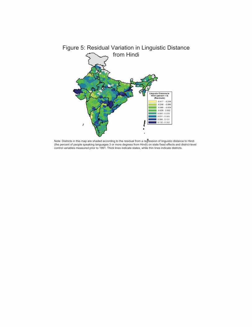
3
Figure 5: Residual Variation in Linguistic Distance from Hindi
Note: Districts in this map are shaded according to the residual from a regression of linguistic distance to Hindi(the percent of people speaking languages 3 or more degrees from Hindi) on state fixed effects and district-level control variables measured prior to 1991. Thick lines indicate states, while thin lines indicate districts.

Table 1: Measures of Linguistic Distance to HindiAverage Across Languages in 1991
Sample Languages Degrees Percent Cognates Nodes0 Degrees
Hindi-Urdu 0 100 0 0.4561 Degree
Gujarati, Punjabi, Rajasthani 1 67.1 5 0.0842 Degrees
Konkani, Marathi 2 56.4 6.5 0.0763 Degrees
Assamese, Bengali, Bihari, Oriya 3 64.1 7 0.1334 Degrees
Kashmiri, Sindhi, Sinhalese 4 53.3 7.3 0.0055 Degrees
All non-Indo European Languages 5 5 12.5 0.244
Sources: Jay Jasanoff (personal communications, 2006), Ethnologue database (2006), Census of India (1991)
Share of Native Speakers

Table 2: Summary StatisticsVariable Num Obs Mean St. Dev. Min. Max. Panel A (at the district level)Degree measure of linguistic distance from native languages to Hindi 390 3.218 1.364 1.001 4.999Percent of people who speak languages at distance > 2 390 0.373 0.443 0.000 1.000Percent of people who speak languages at distance 0 (Hindi/Urdu natives) 390 0.465 0.443 0.000 1.000Percent of people who speak languages at distance 1 390 0.095 0.265 0.000 0.991Percent of people who speak languages at distance 2 390 0.067 0.212 0.000 0.958Percent of people who speak languages at distance 3 390 0.094 0.251 0.000 0.985Percent of people who speak languages at distance 4 390 0.013 0.069 0.000 0.766Percent of people who speak languages at distance 5 390 0.265 0.391 0.000 1.000Percent of people native in English 390 0.00013 0.00049 0.000 0.00670
Percent of urban schools that teach in mother tongue*: Primary 408 0.889 0.222 0.000 1.078Upper primary 408 0.840 0.245 0.000 1.022
Panel B (at the state level, only urban areas)Percent of schools that teach English**: Primary 32 0.263 0.164 0.023 0.664
Upper primary 32 0.310 0.070 0.233 0.511Secondary 32 0.337 0.104 0.182 0.615
Percent of schools with English instruction: Primary 32 0.222 0.237 0.000 1.000Upper primary 32 0.321 0.268 0.053 1.000Secondary 32 0.380 0.285 0.047 1.000Higher secondary 31 0.470 0.295 0.051 1.000
* The percent of schools teaching in the mother tongue can be greater than 1 due to noise in the data.** Note that the numbers in the text differ since these are a mean of averages across states, as opposed to a mean across the country.

Dependent Variable:Sample:
Linguistic distance (0 - 5) 0.058 *** 0.014 0.077 ***(0.016) (0.017) (0.017)
Linguistic distance > 2 0.293 *** 0.166 *** 0.349 ***(0.049) (0.061) (0.049)
D1: Linguistic distance = 0 0.249 *** 0.319 *** 0.307 *** -0.027 0.027 0.474 *** 0.438 *** (Hindi/Urdu speakers) (0.057) (0.068) (0.038) (0.068) (0.047) (0.072) (0.038)D2: Linguistic distance = 2 -0.118
(0.098)D3: Linguistic distance = 3 0.260 ***
(0.071)D4: Linguistic distance = 4 0.229 ***
(0.077)D5: Linguistic distance = 5 0.207 ***
(0.071)Year = 1991 0.209 *** 0.210 *** 0.209 ***
(0.065) (0.065) (0.065)Most spoken language in 0.112 0.089 0.056 0.000 -0.066 0.149 ** 0.126 ** state (0.086) (0.090) (0.074) (0.059) (0.058) (0.074) (0.051)Share of native speakers in 0.448 *** 0.477 *** 0.514 *** 0.407 *** 0.495 *** 0.491 *** 0.512 *** state (0.112) (0.118) (0.103) (0.078) (0.085) (0.093) (0.071)
Obs (weighted, in millions) 1E+09 1E+09 1E+09 4E+08 4E+08 8E+08 8E+08Observations 1085 1085 1085 537 537 548 548R-squared 0.809 0.797 0.807 0.887 0.897 0.938 0.950Test: D1=0, D2=0, D3=0, D4=0, D5=0 (p-value) 0.000
Dependent var. mean (weighted) 0.55 0.55 0.55 0.41 0.41 0.62 0.62
(7)
% of Multilinguals who Learn EnglishBoth Years (1961 and 1991)
Note: This table displays estimates of equation (1). Observations are at the state-mother tongue level. The dependent variable is the percent of native speakers who choose to learn English (conditional on being multilingual). The primary independent variables are measures of the linguistic distance between the native language and Hindi. All columns include an indicator for whether the native language is the state's primary language, the share of native speakers in the state and state fixed effects. Columns 1-4 include year fixed effects, while columns 5-6 (7-8) include only observations from 1961 (1991). In column 1, the omitted group has a linguistic distance of 1 degree away from Hindi. Observations are weighted by the number of native speakers in the state. All columns exclude observations with zero multilinguals and observations where the native language is English; these account for an extremely small number of individuals. Robust standard errors, clustered by state-language, are shown in parentheses. *** 1%, ** 5%, * 10%
(1) (4) (6)
Table 3: Impact of Linguistic Distance on Percent of Native Speakers who Learn English
(2) (3)1961 1991
(5)

Dependent Variable:
Linguistic distance 0.336 *** 0.199 *** (weighted average) (0.105) (0.038)Percent distant speakers 1.061 0.479 (>2 degrees) (1.028) (0.391)Percent speakers at 0 -0.203 0.297 ** -0.130 0.163 *** (Hindi/Urdu speakers) (0.163) (0.131) (0.083) (0.054)Hindi belt states -0.189 0.998 -0.280 * 0.323
(0.211) (0.752) (0.140) (0.218)
Observations 119 119 90 90R-squared 0.726 0.678 0.672 0.576
Dependent var. mean 0.340 0.340 0.303 0.303
Table 4: Impact of Linguistic Distance on Percent of Schools that Teach English% of Schools Teaching
In English% of Schools Teaching
English
Note: This table displays estimates of equation (2). Observations are at the state-school type (primary, upper primary, secondary or higher secondary) level. The dependent variable is the percent of schools in the state that teach in English (columns 1 and 2) or teach English as a second language (columns 3 and 4). The primary independent variables are measures of the linguistic distance from Hindi of languages spoken in the state; the first row presents coefficients of the weighted average across all languages spoken, while the second row presents coefficients of the percent of speakers at least 3 degrees away from Hindi. All columns include fixed effects for region and school type, the percent of native English speakers, the percent of native Hindi/Urdu speakers, a dummy for a Hindi belt state, child population in 1991, household wage income, average wage income for an educated individual, distance to the closest big city, a dummy for a coastline and the percent of people who: have college degrees or secondary school degrees, are literate, are Muslim, ride a train and the percent of households with electricity. Robust standard errors, clustered by state, are shown in parentheses. Critical values are adjusted for the small number of states in the data. *** 1%, ** 5%, * 10%
(1) (2) (3) (4)

Level of Observation:
Dependent variable:
Linguistic distance measure:
Panel ALinguistic distance 0.037 ** 0.328 *** 0.035 0.436 *** 0.180 ** 2.228 ***
(0.018) (0.127) (0.025) (0.167) (0.092) (0.839)Percent speakers at 0 -0.201 *** -0.010 -0.247 ** -0.008 -1.428 ** -0.204 (Hindi/Urdu speakers) (0.076) (0.077) (0.110) (0.123) (0.583) (0.425)Number of IITs and NIITs 0.159 *** 0.157 *** 0.161 0.157 0.662 ** 0.643 **
(0.062) (0.062) (0.117) (0.117) (0.357) (0.346)
Observations 1840 1840 1840 1840 1840 1840R-squared 0.44 0.44 0.39 0.39 0.44 0.44 Panel BLinguistic distance 0.039 ** 0.306 ** 0.032 0.345 ** 0.183 * 1.985 **
(0.018) (0.126) (0.026) (0.168) (0.094) (0.857)Big city * Linguistic -0.063 * -0.241 0.425 ** 1.553 ** 0.498 1.797 distance (0.037) (0.167) (0.170) (0.753) (0.399) (1.714)Big city 0.492 *** 0.417 *** 1.585 * 2.146 *** 3.272 3.962 **
(0.140) (0.118) (0.914) (0.815) (2.121) (1.834)Percent speakers at 0 -0.194 ** -0.010 -0.239 ** -0.039 -1.383 ** -0.249 (Hindi/Urdu speakers) (0.078) (0.078) (0.115) (0.125) (0.615) (0.433)Big city * Percent speakers at 0 0.158 0.094 -1.912 *** -1.350 -2.331 -1.582 (Hindi/Urdu speakers) (0.130) (0.142) (0.725) (0.988) (1.631) (2.196)Number of IITs and NIITs 0.136 *** 0.133 *** 0.007 -0.003 0.302 ** 0.266 **
(0.058) (0.058) (0.127) (0.130) (0.359) (0.356)
Observations 1890 1890 1890 1890 1890 1890R-squared 0.52 0.52 0.74 0.74 0.63 0.63Mean of dependent variable 0.151 0.151 0.252 0.252 0.810 0.810
District-Year
Weighted average
Percent distant
Weighted average
Percent distant
Percent distant
(Log) Number of HQ & Branches
(Log) Number of Employees per Branch
Weighted average
Note: This table displays estimates of equation (3). Observations are at the district-year level and includes data from 1995, 1998, 1999, 2002 and 2003. The dependent variable is an indicator for the existence of any IT headquarters or branch in the district (columns 1-2), the log of the number of headquarters and branches (columns 3-4) and the log of the number of employees per branch (columns 5-6). When calculating logs, I add 1 to avoid dropping districts with no IT presence. The primary independent variable is a measure of the linguistic distance from Hindi of languages spoken in the district; odd columns use the weighted average across all languages spoken, while even columns use the percent of speakers at least 3 degrees away from Hindi. In Panel A, I drop observations for the ten most populous cities in India and in Panel B, I include them but also include interactions. All columns include fixed effects for state and year. Other controls include log of population, fraction of the district that is urbanized, the percent of native English speakers, the percent of native Hindi/Urdu speakers, household wage income, average wage income for an educated individual, distance to the closest big city, distance to closest airport, the number of elite engineering colleges, a dummy for a coastline and the percent of people who: have regular jobs, have college degrees or secondary school degrees or engineering degrees, are literate, are Muslim, ride a train and the percent of households with electricity. Robust standard errors, clustered by district, are shown in parentheses. *** 1%, ** 5%, * 10%
(3) (4) (5)
Table 5: Impact of Linguistic Distance on Growth of IT presence
Any HQ or branch
(1) (2) (6)

Table 6: Impact of Linguistic Distance on Grade School Enrollment (continued on next page)Level of Observation:
Girls Boys Girls Boys Girls Boys Girls Boys
Panel A: Weighted averagePost * Linguistic distance 0.066 *** 0.070 *** 0.040 * 0.020 0.066 *** 0.049 ** 0.117 ** 0.120 **
(0.024) (0.024) (0.020) (0.019) (0.022) (0.022) (0.051) (0.050)Post * Percent speakers at 0 0.151 * 0.045 0.228 *** 0.192 ** 0.192 0.109 -0.025 -0.114 (Hindi/Urdu speakers) (0.088) (0.074) (0.079) (0.076) (0.133) (0.080) (0.146) (0.150)Post * Hindi belt states -0.062 -0.010 -0.279 *** -0.289 *** -0.452 *** -0.335 *** 0.283 0.503 ***
(0.096) (0.084) (0.083) (0.077) (0.106) (0.080) (0.178) (0.195)
Observations 8509 8660 3605 3635 2112 2157 2792 2868R-squared 0.745 0.706 0.930 0.923 0.942 0.931 0.794 0.753
Panel B: Percent distant speakersPost * Linguistic distance 0.348 ** 0.296 * 0.324 ** 0.268 ** 0.539 *** 0.328 ** 0.283 0.306
(0.175) (0.174) (0.163) (0.133) (0.178) (0.136) (0.290) (0.381)Post * Percent speakers at 0 0.302 *** 0.190 *** 0.343 *** 0.274 *** 0.374 *** 0.241 *** 0.179 0.090 (Hindi/Urdu speakers) (0.089) (0.070) (0.097) (0.090) (0.145) (0.090) (0.125) (0.121)Post * Hindi belt states 0.131 0.151 -0.092 -0.131 -0.140 -0.150 0.422 ** 0.659 **
(0.141) (0.148) (0.109) (0.089) (0.127) (0.113) (0.199) (0.307)
Observations 8509 8660 3605 3635 2112 2157 2792 2868R-squared 0.745 0.706 0.930 0.924 0.942 0.931 0.794 0.753Mean enrollment by grade/gender in 1993 4817 5685 6066 6807 5184 6103 2867 3926
(3)(1) (2) (8)(4) (6)
District-Year-Grade
(5)
Primary (Grades 1-5) Upper Primary (Grades 6-8) Secondary (Grades 9-12)
(7)
Sample: All Grades
Note: This table displays estimates of equation (4). Observations are at the district-year-grade level. The dependent variable is the log change in the number of children enrolled in the grade in the district from 1987 to 1993 (time period 'pre') or 1993 to 2002 (time period 'post'). The primary independent variable is a measure of the linguistic distance from Hindi of languages spoken in the district interacted with an indicator variable for the time period post reforms; panels A and C use the weighted average across all languages spoken, while panels B and D use the percent of speakers at least 3 degrees away from Hindi. All columns include fixed effects for district, timeperiod and grade and region interacted with post (panels A and B) or state interacted with post (panels C and D). Other controls include log enrollment in the pre year, log child population in pre and post years, urbanization in pre and post years, a proxy for labor demand growth and post interacted with: the percent of native English speakers, the percent of native Hindi/Urdu speakers, a dummy for a Hindi belt state, household wage income, average wage income for an educated individual, distance to the closest big city, a dummy for a coastline and the percent of people who: have regular jobs, have college degrees or secondary school degrees, are literate, are Muslim, ride a train and the percent of households with electricity. Robust standard errors, clustered by district, are shown in parentheses. *** 1%, ** 5%, * 10%

Table 6 (continued): Impact of Linguistic Distance on Grade School EnrollmentLevel of Observation:
Girls Boys Girls Boys Girls Boys Girls Boys
Panel C: Weighted averagePost * Linguistic distance 0.038 0.050 * 0.022 0.014 0.054 ** 0.046 * 0.084 0.085
(0.027) (0.028) (0.021) (0.020) (0.027) (0.026) (0.055) (0.057)Post * Percent speakers at 0 0.038 -0.009 0.105 0.008 -0.084 -0.069 -0.078 0.072 (Hindi/Urdu speakers) (0.101) (0.090) (0.080) (0.089) (0.106) (0.091) (0.208) (0.225)
Observations 8509 8660 3605 3635 2112 2157 2792 2868R-squared 0.751 0.714 0.942 0.938 0.950 0.944 0.807 0.767
Panel C: Percent distant speakersPost * Linguistic distance 0.068 0.001 0.064 -0.051 0.284 * 0.074 0.000 -0.100
(0.151) (0.146) (0.140) (0.139) (0.155) (0.133) (0.259) (0.351)Post * Percent speakers at 0 0.099 0.027 0.152 -0.006 0.105 -0.003 -0.028 0.081 (Hindi/Urdu speakers) (0.087) (0.087) (0.107) (0.134) (0.110) (0.110) (0.180) (0.233)
Observations 8509 8660 3605 3635 2112 2157 2792 2868R-squared 0.751 0.714 0.942 0.938 0.950 0.944 0.807 0.767Mean enrollment by grade/gender in 1993 4817 5685 6066 6807 5184 6103 2867 3926
(7) (8)
Note: This table displays estimates of equation (4). Observations are at the district-year-grade level. The dependent variable is the log change in the number of children enrolled in the grade in the district from 1987 to 1993 (time period 'pre') or 1993 to 2002 (time period 'post'). The primary independent variable is a measure of the linguistic distance from Hindi of languages spoken in the district interacted with an indicator variable for the time period post reforms; panels A and C use the weighted average across all languages spoken, while panels B and D use the percent of speakers at least 3 degrees away from Hindi. All columns include fixed effects for district, timeperiod and grade and region interacted with post (panels A and B) or state interacted with post (panels C and D). Other controls include log enrollment in the pre year, log child population in pre and post years, urbanization in pre and post years, a proxy for labor demand growth and post interacted with: the percent of native English speakers, the percent of native Hindi/Urdu speakers, a dummy for a Hindi belt state, household wage income, average wage income for an educated individual, distance to the closest big city, a dummy for a coastline and the percent of people who: have regular jobs, have college degrees or secondary school degrees, are literate, are Muslim, ride a train and the percent of households with electricity. Robust standard errors, clustered by district, are shown in parentheses. *** 1%, ** 5%, * 10%
(1) (2) (3) (4) (5) (6)
District-Year-Grade
Sample: All Grades Primary (Grades 1-5) Upper Primary (Grades 6-8) Secondary (Grades 9-12)

Level of Observation:Dependent variable:
Linguistic distance measure:
English * Linguistic Distance 0.084 *** 0.339 *** 0.033 *** 0.137 ***(0.013) (0.052) (0.009) (0.037)
-- * 2004 0.040 *** 0.168 ***(0.013) (0.058)
-- * 2005 0.060 *** 0.281 ***(0.015) (0.065)
-- * 2006 0.064 *** 0.235 ***(0.016) (0.064)
-- * 2007 0.075 *** 0.241 ***(0.016) (0.062)
English * Percent speakers at 0 0.150 ** 0.334 *** 0.315 *** 0.399 *** (Hindi/Urdu) (0.071) (0.067) (0.073) (0.074)
p-values from F-tests: all English * Linguistic Distance Variables (p-value) 0.000 0.000Observations 5086 5086 5086 5086R-squared 0.699 0.698 0.703 0.702
Dependent var. mean 0.366 0.366 0.366 0.366Note: This table displays estimates of equation (5). Observations are at the district-year-language of instruction level. The dependent variable is enrollment of children in grades 1-8 divided by the relevant child population (from the same datasource). The primary independent variable is a measure of the linguistic distance from Hindi of languages spoken in the district interacted with an indicator variable for English as the medium of instruction; odd columns use the weighted average across all languages spoken, while even columns use the percent of speakers at least 3 degrees away from Hindi. All columns include fixed effects for district, language and state interacted with year. Other controls include child population, and interactions of language fixed effects with: the percent of native English speakers, the percent of native Hindi/Urdu speakers, and a dummy variable for whether a district is in the Hindi Belt. All two way interactions for the triple interactions and triple interactions between English as a medium of instruction, the percent of native Hindi/Urdu speakers and time dummies are also included in columns 3 and 4. Robust standard errors, clustered by district, are shown in parentheses. *** 1%, ** 5%, * 10%
Table 7: Impact of Linguistic Distance on Enrollment by Language of Instruction (English, Hindi/Urdu or Others)
District-Year-LanguageEnrollment / Child Population
Weighted average
Percent distant speakers
Weighted average
Percent distant speakers
(1) (2) (3) (4)

Level of Observation:Linguistic distance measure:Sample:
Post * Linguistic distance 0.013 0.017 -0.054 -0.020 0.018 -0.123 -0.011 -0.554 -0.024 -0.175(0.032) (0.031) (0.071) (0.043) (0.033) (0.180) (0.174) (0.393) (0.235) (0.193)
-- * High school -0.047 ** -0.048 *** -0.041 -0.034 -0.052 *** -0.103 -0.126 -0.118 -0.062 -0.103(0.018) (0.018) (0.047) (0.022) (0.020) (0.079) (0.079) (0.179) (0.085) (0.086)
-- * College -0.032 * -0.027 -0.046 -0.027 -0.037 * -0.005 -0.005 -0.015 -0.048 -0.016(0.018) (0.017) (0.041) (0.029) (0.021) (0.073) (0.071) (0.166) (0.110) (0.091)
Post * Percent speakers at 0 -0.070 -0.069 0.166 0.023 -0.063 -0.176 -0.094 -0.262 -0.021 -0.213 (Hindi/Urdu) (0.098) (0.094) (0.255) (0.147) (0.105) (0.165) (0.168) (0.347) (0.209) (0.174) -- * High school 0.043 0.014 0.236 -0.128 0.125 * 0.023 -0.023 0.203 -0.127 0.108
(0.062) (0.063) (0.223) (0.085) (0.073) (0.083) (0.085) (0.251) (0.098) (0.096) -- * College -0.007 -0.011 -0.022 -0.007 0.029 0.023 0.013 0.030 -0.005 0.053
(0.053) (0.056) (0.145) (0.115) (0.066) (0.072) (0.075) (0.184) (0.131) (0.093)Post 1.244 *** 1.201 *** 1.606 *** 1.553 *** 1.137 *** 1.407 *** 1.280 *** 1.839 *** 1.468 *** 1.376 ***
(0.173) (0.168) (0.379) (0.232) (0.184) (0.173) (0.169) (0.377) (0.224) (0.185) -- * High school 0.079 0.110 -0.033 -0.027 0.125 -0.021 0.021 -0.109 -0.113 * 0.005
(0.078) (0.078) (0.188) (0.086) (0.084) (0.067) (0.067) (0.143) (0.065) (0.074) -- * College 0.170 ** 0.173 ** 0.110 -0.036 0.226 ** 0.061 0.081 -0.050 -0.105 0.108
(0.072) (0.071) (0.165) (0.110) (0.088) (0.061) (0.059) (0.137) (0.077) (0.079)High school 0.537 *** 0.426 *** 1.182 *** 0.435 *** 0.589 *** 0.635 *** 0.497 *** 1.268 *** 0.473 *** 0.733 ***
(0.060) (0.057) (0.106) (0.068) (0.069) (0.054) (0.050) (0.084) (0.052) (0.064)College 1.016 *** 0.889 *** 1.586 *** 0.972 *** 1.036 *** 1.118 *** 0.961 *** 1.717 *** 1.008 *** 1.177 ***
(0.052) (0.051) (0.121) (0.075) (0.061) (0.040) (0.040) (0.109) (0.057) (0.047)
Obs. (in millions, weighted) 67.2 55.6 11.6 21.6 45.6 67.2 55.6 11.6 21.6 45.6Observations 71255 58631 12624 22196 49059 71255 58631 12624 22196 49059R-squared 0.671 0.668 0.686 0.649 0.671 0.671 0.668 0.686 0.649 0.671
Dependent var. mean 5.812 5.900 5.406 5.407 5.996 5.812 5.900 5.406 5.407 5.996
Individual
Age > 29All Men Women Age < 30
Note: This table displays estimates of equation (6). Observations are at the individual level using data from 1987 (pre) and 1999 (post). The dependent variable is the log weekly wage and the primary independent variables are measures of the linguistic distance from Hindi of languages spoken in the district interacted with fixed effects for high school completion and college completion; odd columns use the weighted average across all languages spoken, while even columns use the percent of speakers at least 3 degrees away from Hindi. All columns include fixed effects for district, year and state interacted with post. Individual-level controls include age, age squared, married, male, whether the individual has ever moved, whether the individual is self-employed and high school and college also interacted with post and the percent native Hindi speakers. District-level controls include a proxy for labor demand growth and post interacted with: the percent of native English speakers, distance to the closest big city, and a dummy for a coastline. Robust standard errors, clustered by district, are shown in parentheses. *** 1%, ** 5%, * 10%
(4) (5) (9) (10)(2) (3) (7) (8)
Table 8: Impact of Linguistic Distance on Wages and Returns to Education
Weighted average Percent distant speakers
(1) (6)All Men Women Age < 30 Age > 29

Table 9: Impact of Linguistic Distance on Grade School Enrollment in 1993Level of Observation:
Girls Boys Girls Boys Girls Boys Girls Boys
Panel A: Weighted averageLinguistic distance -0.013 -0.030 0.035 0.038 * 0.005 -0.012 -0.101 -0.124 **
(0.029) (0.030) (0.022) (0.023) (0.025) (0.026) (0.062) (0.059)
Observations 4105 4256 1770 1800 1011 1056 1324 1400R-squared 0.678 0.606 0.831 0.783 0.860 0.824 0.610 0.554
Panel B: Percent distant speakersLinguistic distance 0.073 0.103 0.187 0.225 0.122 0.172 -0.076 -0.135
(0.198) (0.206) (0.187) (0.186) (0.175) (0.135) (0.337) (0.421)
Observations 4105 4256 1770 1800 1011 1056 1324 1400R-squared 0.678 0.606 0.831 0.783 0.860 0.824 0.608 0.551
Panel C: Weighted averageLinguistic distance 0.011 -0.030 0.000 -0.011 0.006 -0.024 0.009 -0.049
(0.029) (0.030) (0.023) (0.021) (0.027) (0.028) (0.064) (0.060)
Observations 4105 4256 1770 1800 1011 1056 1324 1400R-squared 0.710 0.655 0.881 0.863 0.898 0.886 0.682 0.643
Panel D: Percent distant speakersLinguistic distance 0.087 0.026 0.106 0.113 0.040 0.017 -0.016 -0.033
(0.165) (0.161) (0.139) (0.134) (0.167) (0.152) (0.311) (0.338)
Observations 4105 4256 1770 1800 1011 1056 1324 1400R-squared 0.710 0.654 0.881 0.863 0.898 0.885 0.682 0.643Mean enrollment by grade/gender in 1993 4817 5685 6066 6807 5184 6103 2867 3926
(7) (8)
Note: This table displays estimates of equation (7). Observations are at the district-grade level. The dependent variable is the log change in the number of children enrolled in the grade in the district from 1987 to 1993. The primary independent variable is a measure of the linguistic distance from Hindi of languages spoken in the district; panels A and C use the weighted average across all languages spoken, while panels B and D use the percent of speakers at least 3 degrees away from Hindi. All columns include fixed effects for grade and region (panels A and B) or state (panels C and D). Other controls include log enrollment in the 1987, the percent of native English speakers, the percent of native Hindi/Urdu speakers, a dummy for a Hindi belt state, log child population in pre and post years, urbanization in pre and post years, a proxy for labor demand growth, household wage income, average wage income for an educated individual, distance to the closest big city, a dummy for a coastline and the percent of people who: have regular jobs, have college degrees or secondary school degrees, are literate, are Muslim, ride a train and the percent of households with electricity. Robust standard errors, clustered by district, are shown in parentheses. *** 1%, ** 5%, * 10%
(1) (2) (3) (4) (5) (6)
District-Grade
Sample: All Grades Primary (Grades 1-5) Upper Primary (Grades 6-8) Secondary (Grades 9-12)

Table A1: Summary Statistics on IT Presence Across DistrictsAverage Across All Districts Average Across IT Districts
Year of Data Number of HQ or Branches Employees Number of HQ
or Branches Employees
1995 47 1.36 120 11.83 10431998 47 2.25 279 19.60 24281999 54 2.48 348 18.76 26342002 76 3.24 559 17.46 30062003 72 2.54 604 14.40 3430
Table A2: Summary Statistics on Grade School Enrollment, only urban areas
Grade Mean in 1993Standard
Deviation in 1993
Mean in 2002Standard
Deviation in 2002
Class size / Class size in 1st
grade 1993
Class size / Class size in
1st grade 2002
% Growth since 1993
Grade 1 14698 22274 16948 24595 15%Grade 2 12337 19817 14915 22793 84% 88% 21%Grade 3 11872 19591 14406 22455 81% 85% 21%Grade 4 11118 18543 13689 21336 76% 81% 23%Grade 5 11060 18965 14117 22058 75% 83% 28%Grade 6 11362 18554 14068 23283 77% 83% 24%Grade 7 10211 16239 13316 20667 69% 79% 30%Grade 8 9686 15239 13136 19854 66% 78% 36%Grade 9 9345 13666 12290 17445 64% 73% 32%Grade 10 7492 10560 10643 13841 51% 63% 42%Grade 11 4372 6425 9036 11559 30% 53% 107%Grade 12 4000 5986 8077 9878 27% 48% 102%
Overall: 32%
Number of Disticts with IT (Out of 409)