How to train your ViT? Data, Augmentation,and Regularization in Vision Transformers

Andreas Steiner∗, Alexander Kolesnikov∗, Xiaohua Zhai∗Ross Wightman†, Jakob Uszkoreit, Lucas Beyer∗

Google Research, Brain Team; †independent researcher

{andstein,akolesnikov,xzhai,usz,lbeyer}@google.com, rwightman@gmail.com

Abstract

Vision Transformers (ViT) have been shown to attain highly competitive per-formance for a wide range of vision applications, such as image classification,object detection and semantic image segmentation. In comparison to convolu-tional neural networks, the Vision Transformer’s weaker inductive bias is generallyfound to cause an increased reliance on model regularization or data augmentation(“AugReg” for short) when training on smaller training datasets. We conduct asystematic empirical study in order to better understand the interplay betweenthe amount of training data, AugReg, model size and compute budget. 1 As oneresult of this study we find that the combination of increased compute and AugRegcan yield models with the same performance as models trained on an order ofmagnitude more training data: we train ViT models of various sizes on the publicImageNet-21k dataset which either match or outperform their counterparts trainedon the larger, but not publicly available JFT-300M dataset.

1 Introduction

The Vision Transformer (ViT) [10] has recently emerged as a competitive alternative to convolutionalneural networks (CNNs) that are ubiquitous across the field of computer vision. Without thetranslational equivariance of CNNs, ViT models are generally found to perform best in settings withlarge amounts of training data [10] or to require strong AugReg schemes to avoid overfitting [34]. Toour knowledge, however, so far there was no comprehensive study of the trade-offs between modelregularization, data augmentation, training data size and compute budget in Vision Transformers.

In this work, we fill this knowledge gap by conducting a thorough empirical study. We pre-train alarge collection of ViT models (different sizes and hybrids with ResNets [14]) on datasets of differentsizes, while at the same time performing carefully designed comparisons across different amountsof regularization and data augmentation. We proceed by conducting extensive transfer learningexperiments with the resulting models. We focus mainly on the perspective of a practitioner withlimited compute and data annotation budgets.

The homogeneity of the performed study constitutes one of the key contributions of this paper. Forthe vast majority of works involving Vision Transformers it is not practical to retrain all baselines andproposed methods on equal footing, in particular those trained on larger amounts of data. Furthermore,there are numerous subtle and implicit design choices that cannot be controlled for effectively, suchas the precise implementation of complex augmentation schemes, hyper-parameters (e.g. learning

1We release more than 50’000 ViT models trained under diverse settings on various datasets. We believe thisto be a treasure trove for model analysis. Available at https://github.com/google-research/vision_transformer and https://github.com/rwightman/pytorch-image-models.

Preprint. ∗Equal contribution.

arX

iv:2

106.

1027

0v1

[cs

.CV

] 1

8 Ju

n 20

21

1.28M 1.28M+AugReg 13M 13M+AugReg 300MPre-training dataset size

60%

65%

70%

75%

80%

85%

90%ImageNet top-1 accuracy after fine-tuning

ViT-B/32ViT-B/16ViT-L/16

10 1 100 101 102

Training time [TPUv2 core-hours]

10 1

100

Erro

r

Pet37 (3312 images)

10 1 100 101 102

Training time [TPUv2 core-hours]

10 1

100

Erro

r

Resisc45 (31k images)

Ti/16, from scratchB/16, from scratch

Ti/16, transfer+AugRegB/16, transfer+AugReg

Ti/16, transferB/16, transfer

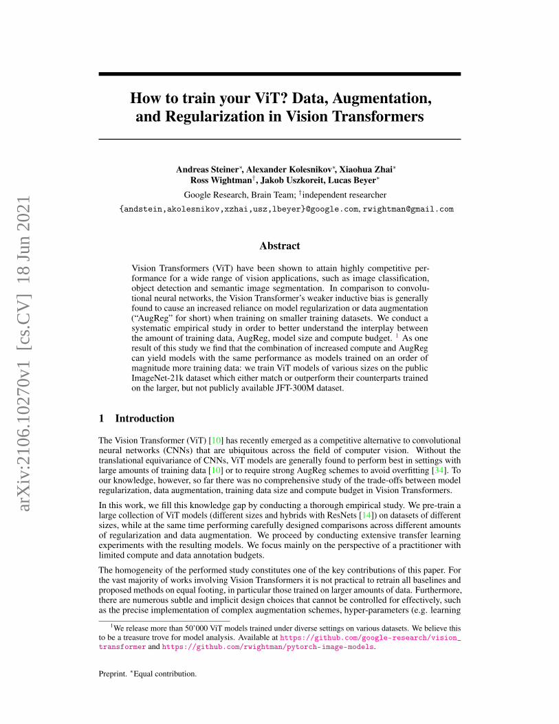
Figure 1: Left: Adding the right amount of regularization and image augmentation can lead to similargains as increasing the dataset size by an order of magnitude. Right: For small and mid-sized datasetsit is very hard to achieve a test error that can trivially be attained by fine-tuning a model pre-trained ona large dataset like ImageNet-21k – see also Figure 2. With our recommended models (Section 4.5),one can find a good solution with very few trials (bordered green dots). Note that AugReg is nothelpful when transferring pre-trained models (borderless green dots).

rate schedule, weight decay), test-time preprocessing, dataset splits and so forth. Such inconsistenciescan result in significant amounts of noise added to the results, quite possibly affecting the ability todraw any conclusions. Hence, all models on which this work reports have been trained and evaluatedin a consistent setup.

The insights we draw from our study constitute another important contribution of this paper. In par-ticular, we demonstrate that carefully selected regularization and augmentations roughly correspond(from the perspective of model accuracy) to a 10x increase in training data size. However, regardlessof whether the models are trained with more data or better AugRegs, one has to spend roughly thesame amount of compute to get models attaining similar performance. We further evaluate if there isa difference between adding data or better AugReg when fine-tuning the resulting models on datasetsof various categories.

In addition, we aim to shed light on other aspects of using Vision Transformers in practice such ascomparing transfer learning and training from scratch for mid-sized datasets. Finally, we evaluatevarious compute versus performance trade-offs. We discuss all of the aforementioned insights andmore in detail in Section 4.

2 Scope of the study

With the ubiquity of modern deep learning [21] in computer vision it has quickly become commonpractice to pre-train models on large datasets once and re-use their parameters as initialization or apart of the model as feature extractors in models trained on a broad variety of other tasks [28, 40].

In this setup, there are multiple ways to characterize computational and sample efficiency. Whensimply considering the overall costs of pre-training and subsequent training or fine-tuning procedurestogether, the cost of pre-training usually dominates, often by orders of magnitude. From the vantagepoint of a researcher aiming to improve model architectures or pre-training schemes, the pre-trainingcosts might therefore be most relevant. Most practitioners, however, rarely, if ever perform pre-training on today’s largest datasets but instead use some of the many publicly available parameter sets.For them the costs of fine-tuning, adaptation or training a task-specific model from scratch would beof most interest.

Yet another valid perspective is that all training costs are effectively negligible since they are amortizedover the course of the deployment of a model in applications requiring a very large number ofinvocations of inference.

In this setup there are different viewpoints on computational and data efficiency aspects. One approachis to look at the overall computational and sample cost of both pre-training and fine-tuning. Normally,“pre-training cost” will dominate overall costs. This interpretation is valid in specific scenarios,

2

especially when pre-training needs to be done repeatedly or reproduced for academic/industrialpurposes. However, in the majority of cases the pre-trained model can be downloaded or, in the worstcase, trained once in a while. Contrary, in these cases, the budget required for adapting this modelmay become the main bottleneck.

Thus, we pay extra attention to the scenario, where the cost of obtaining a pre-trained model is freeor effectively amortized by future adaptation runs. Instead, we concentrate on time and computespent on finding a good adaptation strategy (or on tuning from scratch training setup), which we call"practitioner’s cost".

A more extreme viewpoint is that the training cost is not crucial, and all what matters is eventualinference cost of the trained model, “deployment cost”, which will amortize all other costs. This isespecially true for large scale deployments, where a visual models is executed to be used massivenumber of times. Overall, there are three major viewpoints on what is considered to be the centralcost of training a vision model. In this study we touch on all three of them, but mostly concentrate on“practioner’s” and “deployment” costs.

3 Experimental setup

In this section we describe our unified experimental setup, which is used throughout the paper. We usea single JAX/Flax [15, 3] codebase for pre-training and transfer learning using TPUs. Inference speedmeasurements, however, were obtained on V100 GPUs (16G) using the timm PyTorch library [37].All datasets are accessed through the TensorFlow Datasets library, which helps to ensure consistencyand reproducibility. More details of our setup are provided below.

3.1 Datasets and metrics

For pre-training we use two large-scale image datasets: ILSVRC-2012 (ImageNet-1k) and ImageNet-21k. ImageNet-21k dataset contains approximately 14 million images with about 21’000 distinctobject categories [9, 26]. ImageNet-1k is a subset of ImageNet-21k consisting of about 1.3 milliontraining images and 1000 object categories. We make sure to de-duplicate images in ImageNet-21kwith respect to the test sets of the downstream tasks as described in [10, 18]. Additionally, we usedImageNetV2 [25] for evaluation purposes.

For transfer learning evaluation we use 4 popular computer vision datasets from the VTAB bench-mark [40]: CIFAR-100 [20], Oxford IIIT Pets [24] (or Pets37 for short), Resisc45 [5] and Kitti-distance [11]. We selected these datasets to cover the standard setting of natural image classification(CIFAR-100 and Pets37), as well as classification of images captured by specialized equipment(Resisc45) and geometric tasks (Kitti-distance). In some cases we also use the full VTAB benchmark(19 datasets) to additionally ensure robustness of our findings.

For all datasets we report top-1 classification accuracy as our main metric. Hyper-parameters forfine-tuning are selected by the result from the validation split, and final numbers are reported fromthe test split. Note that for ImageNet-1k we follow common practice of reporting our main resultson the validation set. Thus, we set aside 1% of the training data into a minival split that we use formodel selection. Similarly, we use a minival split for CIFAR-100 (2% of training split) and OxfordIIT Pets (10% of training split). For Resisc45, we use only 60% of the training split for training, andanother 20% for validation, and 20% for computing test metrics. Kitti-distance finally comes with anofficial validation and test split that we use for the intended purpose. See [40] for details about theVTAB dataset splits.

3.2 Models

This study focuses mainly on the Vision Transformer (ViT) [10]. We use 4 different configurationsfrom [10, 34]: ViT-Ti, ViT-S, ViT-B and ViT-L, which span a wide range of different capacities.The details of each configuration are provided in Table 1. We use patch-size 16 for all models, andadditionally patch-size 32 for the ViT-S and ViT-B variants. The only difference to the original ViTmodel [10] in our paper is that we drop the hidden layer in the head, as empirically it does not lead tomore accurate models and often results in optimization instabilities.

3

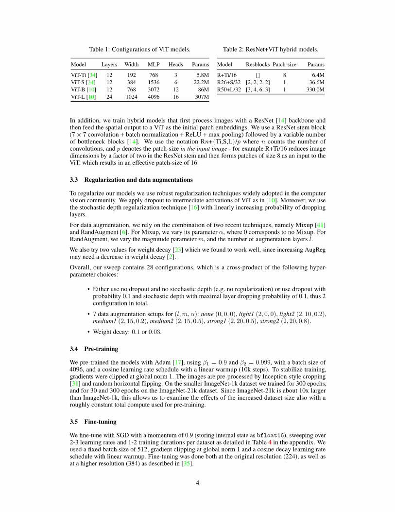
Table 1: Configurations of ViT models.

Model Layers Width MLP Heads Params

ViT-Ti [34] 12 192 768 3 5.8MViT-S [34] 12 384 1536 6 22.2MViT-B [10] 12 768 3072 12 86MViT-L [10] 24 1024 4096 16 307M

Table 2: ResNet+ViT hybrid models.

Model Resblocks Patch-size Params

R+Ti/16 [] 8 6.4MR26+S/32 [2, 2, 2, 2] 1 36.6MR50+L/32 [3, 4, 6, 3] 1 330.0M

In addition, we train hybrid models that first process images with a ResNet [14] backbone andthen feed the spatial output to a ViT as the initial patch embeddings. We use a ResNet stem block(7× 7 convolution + batch normalization + ReLU + max pooling) followed by a variable numberof bottleneck blocks [14]. We use the notation Rn+{Ti,S,L}/p where n counts the number ofconvolutions, and p denotes the patch-size in the input image - for example R+Ti/16 reduces imagedimensions by a factor of two in the ResNet stem and then forms patches of size 8 as an input to theViT, which results in an effective patch-size of 16.

3.3 Regularization and data augmentations

To regularize our models we use robust regularization techniques widely adopted in the computervision community. We apply dropout to intermediate activations of ViT as in [10]. Moreover, we usethe stochastic depth regularization technique [16] with linearly increasing probability of droppinglayers.

For data augmentation, we rely on the combination of two recent techniques, namely Mixup [41]and RandAugment [6]. For Mixup, we vary its parameter α, where 0 corresponds to no Mixup. ForRandAugment, we vary the magnitude parameter m, and the number of augmentation layers l.

We also try two values for weight decay [23] which we found to work well, since increasing AugRegmay need a decrease in weight decay [2].

Overall, our sweep contains 28 configurations, which is a cross-product of the following hyper-parameter choices:

• Either use no dropout and no stochastic depth (e.g. no regularization) or use dropout withprobability 0.1 and stochastic depth with maximal layer dropping probability of 0.1, thus 2configuration in total.

• 7 data augmentation setups for (l,m, α): none (0, 0, 0), light1 (2, 0, 0), light2 (2, 10, 0.2),medium1 (2, 15, 0.2), medium2 (2, 15, 0.5), strong1 (2, 20, 0.5), strong2 (2, 20, 0.8).

• Weight decay: 0.1 or 0.03.

3.4 Pre-training

We pre-trained the models with Adam [17], using β1 = 0.9 and β2 = 0.999, with a batch size of4096, and a cosine learning rate schedule with a linear warmup (10k steps). To stabilize training,gradients were clipped at global norm 1. The images are pre-processed by Inception-style cropping[31] and random horizontal flipping. On the smaller ImageNet-1k dataset we trained for 300 epochs,and for 30 and 300 epochs on the ImageNet-21k dataset. Since ImageNet-21k is about 10x largerthan ImageNet-1k, this allows us to examine the effects of the increased dataset size also with aroughly constant total compute used for pre-training.

3.5 Fine-tuning

We fine-tune with SGD with a momentum of 0.9 (storing internal state as bfloat16), sweeping over2-3 learning rates and 1-2 training durations per dataset as detailed in Table 4 in the appendix. Weused a fixed batch size of 512, gradient clipping at global norm 1 and a cosine decay learning rateschedule with linear warmup. Fine-tuning was done both at the original resolution (224), as well asat a higher resolution (384) as described in [35].

4

100 102 104

Compute budget [TPUv2 core-hours]

0%

20%

40%

60%

80%

100%

Accu

racy

Pet37 (3312 images)

101 103 105

Compute budget [TPUv2 core-hours]

0%

20%

40%

60%

80%

100%

Accu

racy

Resisc45 (31k images)

B/32, from scratch B/16, from scratch B/32, transfer B/16, transfer

Figure 2: Fine-tuning recommended checkpoints leads to better performance with less compute(green), compared to training from scratch with AugReg (blue) – see Figure 1 (right) for individualruns. For a given compute budget (x-axis), choosing random configurations within that budget leadsto varying final performance, depending on choice of hyper parameters (shaded area covers 90%from 1000 random samples, line corresponds to median).

4 Findings

4.1 Scaling datasets with AugReg and compute

One major finding of our study, which is depicted in Figure 1 (left), is that by judicious use ofimage augmentations and model regularization, one can (pre-)train a model to similar accuracy as byincreasing the dataset size by about an order of magnitude. More precisely, our best models trainedon AugReg ImageNet-1k [27] perform about equal to the same models pre-trained on the 10x largerplain ImageNet-21k [27] dataset. Similarly, our best models trained on AugReg ImageNet-21k, whencompute is also increased (e.g. training run longer), match or outperform those from [10] which weretrained on the plain JFT-300M [30] dataset with 25x more images. Thus, it is possible to match theseprivate results with a publicly available dataset, and it is imaginable that training longer and withAugReg on JFT-300M might further increase performance.

Of course, these results cannot hold for arbitrarily small datasets. For instance, according to Table 5of [39], training a ResNet50 on only 10% of ImageNet-1k with heavy data augmentation improvesresults, but does not recover training on the full dataset.

4.2 Transfer is the better option

Here, we investigate whether, for reasonably-sized datasets a practitioner might encounter, it isadvisable to try training from scratch with AugReg, or whether time and money is better spenttransferring pre-trained models that are freely available. The result is that, for most practical purposes,transferring a pre-trained model is both more cost-efficient and leads to better results.

We perform a thorough search for a good training recipe2 for both the small ViT-Ti/16 and the largerViT-B/16 models on two datasets of practical size: Pet37 contains only about 3000 training imagesand is relatively similar to the ImageNet-1k dataset. Resisc45 contains about 30’000 training imagesand consists of a very different modality of satellite images, which is not well covered by eitherImageNet-1k or ImageNet-21k. Figure 1 (right) and Figure 2 show the result of this extensive search.

The most striking finding is that, no matter how much training time is spent, for the tiny Pet37 dataset,it does not seem possible to train ViT models from scratch to reach accuracy anywhere near that oftransferred models. Furthermore, since pre-trained models are freely available for download, thepre-training cost for a practitioner is effectively zero, only the compute spent on transfer matters, andthus transferring a pre-trained model is simultaneously significantly cheaper.

For the larger Resisc45 dataset, this result still holds, although spending two orders of magnitudemore compute and performing a heavy search may come close (but not reach) to the accuracy ofpre-trained models.

2Not only do we further increase available AugReg settings, but we also sweep over other generally importanttraining hyperparameters: learning-rate, weight-decay, and training duration, as described in Section A in theAppendix.

5

103104

Inference speed [img/sec]

85%

90%

Natural datasets

103104

Inference speed [img/sec]

88%

90%

92%

Specialized datasets

INet21k 300epINet21k 30epINet1k 300ep

103104

Inference speed [img/sec]

75%

80%

Structured datasets

S/32

B/32

R26S

S/16

R50L

B/16

L/16

S/32

B/32

R26S

S/16

R50L

B/16

L/16

S/32

B/32

R26S

S/16

R50L

B/16

L/16

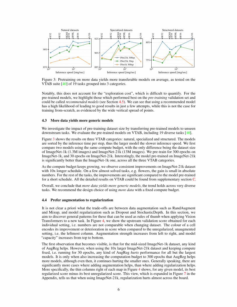
Figure 3: Pretraining on more data yields more transferable models on average, as tested on theVTAB suite [40] of 19 tasks grouped into 3 categories.

Notably, this does not account for the “exploration cost”, which is difficult to quantify. For thepre-trained models, we highlight those which performed best on the pre-training validation set andcould be called recommended models (see Section 4.5). We can see that using a recommended modelhas a high likelihood of leading to good results in just a few attempts, while this is not the case fortraining from-scratch, as evidenced by the wide vertical spread of points.

4.3 More data yields more generic models

We investigate the impact of pre-training dataset size by transferring pre-trained models to unseendownstream tasks. We evaluate the pre-trained models on VTAB, including 19 diverse tasks [40].

Figure 3 shows the results on three VTAB categories: natural, specialized and structured. The modelsare sorted by the inference time per step, thus the larger model the slower inference speed. We firstcompare two models using the same compute budget, with the only difference being the dataset sizeof ImageNet-1k (1.3M images) and ImageNet-21k (13M images). We pre-train for 300 epochs onImageNet-1k, and 30 epochs on ImageNet-21k. Interestingly, the model pre-trained on ImageNet-21kis significantly better than the ImageNet-1k one, across all the three VTAB categories.

As the compute budget keeps growing, we observe consistent improvements on ImageNet-21k datasetwith 10x longer schedule. On a few almost solved tasks, e.g. flowers, the gain is small in absolutenumbers. For the rest of the tasks, the improvements are significant compared to the model pre-trainedfor a short schedule. All the detailed results on VTAB could be found from supplementary section C.

Overall, we conclude that more data yields more generic models, the trend holds across very diversetasks. We recommend the design choice of using more data with a fixed compute budget.

4.4 Prefer augmentation to regularization

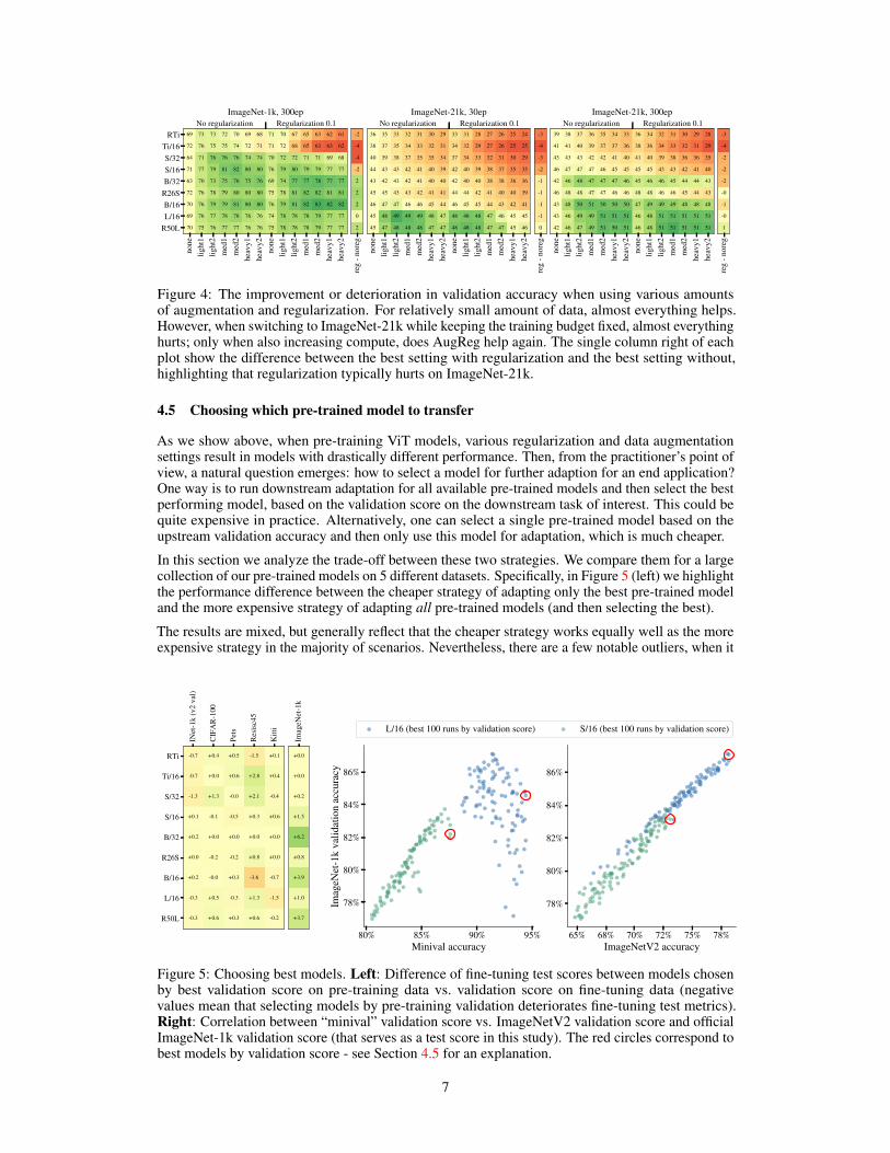
It is not clear a priori what the trade-offs are between data augmentation such as RandAugmentand Mixup, and model regularization such as Dropout and StochasticDepth. In this section, weaim to discover general patterns for these that can be used as rules of thumb when applying VisionTransformers to a new task. In Figure 4, we show the upstream validation score obtained for eachindividual setting, i.e. numbers are not comparable when changing dataset. The colour of a cellencodes its improvement or deterioration in score when compared to the unregularized, unaugmentedsetting, i.e. the leftmost column. Augmentation strength increases from left to right, and model“capacity” increases from top to bottom.

The first observation that becomes visible, is that for the mid-sized ImageNet-1k dataset, any kindof AugReg helps. However, when using the 10x larger ImageNet-21k dataset and keeping computefixed, i.e. running for 30 epochs, any kind of AugReg hurts performance for all but the largestmodels. It is only when also increasing the computation budget to 300 epochs that AugReg helpsmore models, although even then, it continues hurting the smaller ones. Generally speaking, there aresignificantly more cases where adding augmentation helps, than where adding regularization helps.More specifically, the thin columns right of each map in Figure 4 shows, for any given model, its bestregularized score minus its best unregularized score. This view, which is expanded in Figure 7 in theAppendix, tells us that when using ImageNet-21k, regularization hurts almost across the board.

6

none

light

1lig

ht2

med

1m

ed2

heav

y1he

avy2

none

light

1lig

ht2

med

1m

ed2

heav

y1he

avy2

RTiTi/16S/32S/16B/32

R26SB/16L/16

R50L

69 73 73 72 70 69 68 71 70 67 65 63 62 61

72 76 75 75 74 72 71 71 72 68 65 63 63 62

64 71 76 76 76 74 74 70 72 72 71 71 69 68

71 77 79 81 82 80 80 76 79 80 79 79 77 77

63 70 73 75 76 75 76 69 74 77 77 78 77 77

72 76 78 79 80 80 80 75 78 81 82 82 81 81

70 76 79 79 81 80 80 76 79 81 82 83 82 82

69 76 77 78 78 76 76 74 78 78 78 79 77 77

70 75 76 77 77 76 76 75 78 78 78 79 77 77

No regularization Regularization 0.1ImageNet-1k, 300ep

reg

- nor

eg

-2

-4

-4

-2

2

2

2

0

2

none

light

1lig

ht2

med

1m

ed2

heav

y1he

avy2

none

light

1lig

ht2

med

1m

ed2

heav

y1he

avy2

36 35 33 32 31 30 29 33 31 28 27 26 25 24

38 37 35 34 33 32 31 34 32 29 27 26 25 25

40 39 38 37 35 35 34 37 34 33 32 31 30 29

44 43 43 42 41 40 39 42 40 39 38 37 35 35

43 42 43 42 41 40 40 42 40 40 38 38 36 36

45 45 43 43 42 41 41 44 44 42 41 40 40 39

46 47 47 46 46 45 44 46 45 45 44 43 42 41

45 48 49 49 49 48 47 48 48 48 47 46 45 45

45 47 48 48 48 47 47 48 48 48 47 47 45 46

No regularization Regularization 0.1ImageNet-21k, 30ep

reg

- nor

eg

-3

-4

-3

-2

-1

-1

-1

-1

0

none

light

1lig

ht2

med

1m

ed2

heav

y1he

avy2

none

light

1lig

ht2

med

1m

ed2

heav

y1he

avy2

39 38 37 36 35 34 33 36 34 32 31 30 29 28

41 41 40 39 37 37 36 38 36 34 33 32 31 29

43 43 43 42 42 41 40 41 40 39 38 36 36 35

46 47 47 47 46 45 45 45 45 43 43 42 41 40

42 46 48 47 47 47 46 45 46 46 45 44 44 43

46 48 48 47 47 46 46 48 48 46 46 45 44 43

43 48 50 51 50 50 50 47 49 49 49 48 48 48

43 46 49 49 51 51 51 46 48 51 51 51 51 51

42 46 47 49 51 50 51 46 48 51 51 51 51 51

No regularization Regularization 0.1ImageNet-21k, 300ep

reg

- nor

eg

-3

-4

-2

-2

-2

-0

-1

-0

1

Figure 4: The improvement or deterioration in validation accuracy when using various amountsof augmentation and regularization. For relatively small amount of data, almost everything helps.However, when switching to ImageNet-21k while keeping the training budget fixed, almost everythinghurts; only when also increasing compute, does AugReg help again. The single column right of eachplot show the difference between the best setting with regularization and the best setting without,highlighting that regularization typically hurts on ImageNet-21k.

4.5 Choosing which pre-trained model to transfer

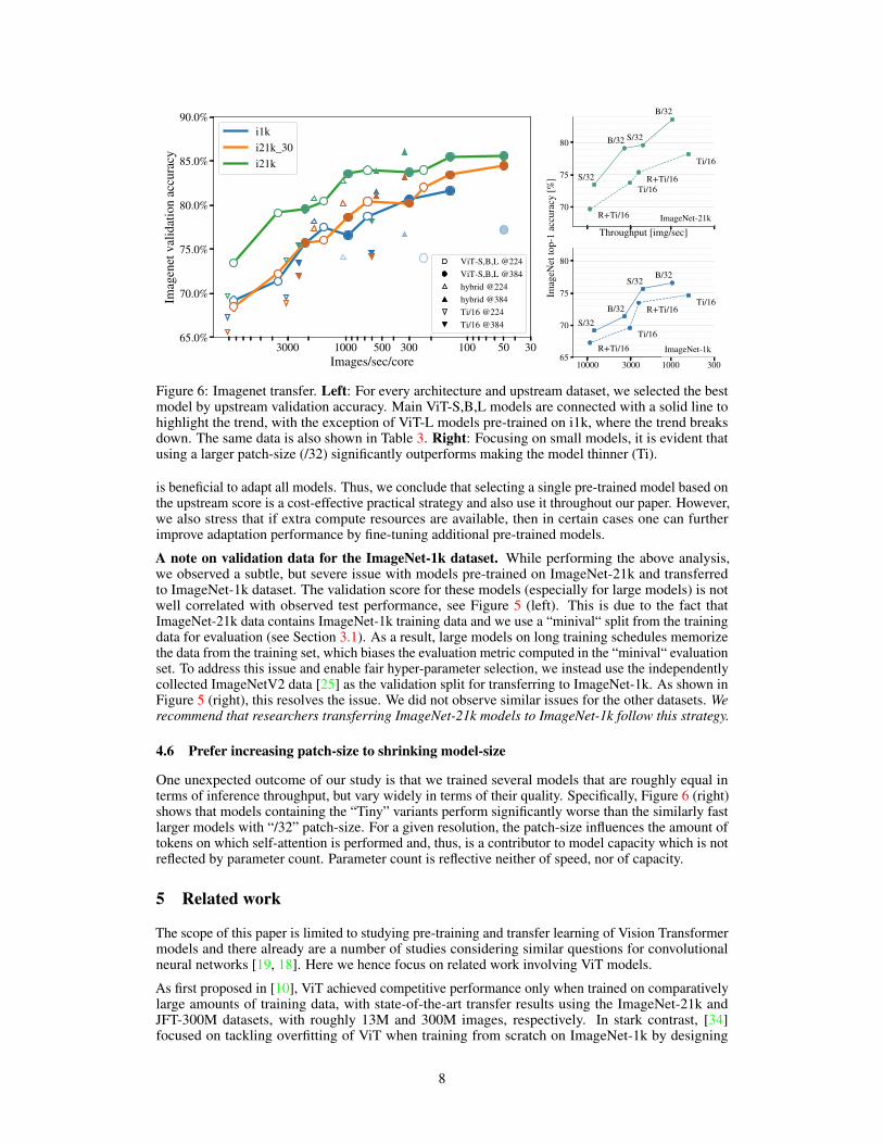
As we show above, when pre-training ViT models, various regularization and data augmentationsettings result in models with drastically different performance. Then, from the practitioner’s point ofview, a natural question emerges: how to select a model for further adaption for an end application?One way is to run downstream adaptation for all available pre-trained models and then select the bestperforming model, based on the validation score on the downstream task of interest. This could bequite expensive in practice. Alternatively, one can select a single pre-trained model based on theupstream validation accuracy and then only use this model for adaptation, which is much cheaper.

In this section we analyze the trade-off between these two strategies. We compare them for a largecollection of our pre-trained models on 5 different datasets. Specifically, in Figure 5 (left) we highlightthe performance difference between the cheaper strategy of adapting only the best pre-trained modeland the more expensive strategy of adapting all pre-trained models (and then selecting the best).

The results are mixed, but generally reflect that the cheaper strategy works equally well as the moreexpensive strategy in the majority of scenarios. Nevertheless, there are a few notable outliers, when it

INet-

1k (v

2 va

l)

CIFA

R-10

0

Pets

Resis

c45

Kitti

RTi

Ti/16

S/32

S/16

B/32

R26S

B/16

L/16

R50L

-0.7 +0.4 +0.5 -1.5 +0.1

-0.7 +0.0 +0.6 +2.8 +0.4

-1.3 +1.3 -0.0 +2.1 -0.4

+0.1 -0.1 -0.5 +0.3 +0.6

+0.2 +0.0 +0.0 +0.0 +0.0

+0.0 -0.2 -0.2 +0.8 +0.0

+0.2 -0.0 +0.3 -3.6 -0.7

-0.3 +0.5 -0.3 +1.3 -1.5

-0.3 +0.6 +0.3 +0.6 -0.2

Imag

eNet-

1k

+0.0

+0.0

+0.2

+1.5

+6.2

+0.8

+3.9

+1.0

+3.7

80% 85% 90% 95%Minival accuracy

78%

80%

82%

84%

86%

Imag

eNet-

1k v

alida

tion

accu

racy

65% 68% 70% 72% 75% 78%ImageNetV2 accuracy

78%

80%

82%

84%

86%

L/16 (best 100 runs by validation score) S/16 (best 100 runs by validation score)

Figure 5: Choosing best models. Left: Difference of fine-tuning test scores between models chosenby best validation score on pre-training data vs. validation score on fine-tuning data (negativevalues mean that selecting models by pre-training validation deteriorates fine-tuning test metrics).Right: Correlation between “minival” validation score vs. ImageNetV2 validation score and officialImageNet-1k validation score (that serves as a test score in this study). The red circles correspond tobest models by validation score - see Section 4.5 for an explanation.

7

305010030050010003000Images/sec/core

65.0%

70.0%

75.0%

80.0%

85.0%

90.0%

Imag

enet

valid

ation

accu

racy

ViT-S,B,L @224ViT-S,B,L @384hybrid @224hybrid @384Ti/16 @224Ti/16 @384

i1ki21k_30i21k

Throughput [img/sec]

70

75

80

B/32

S/32B/32

S/32Ti/16

R+Ti/16Ti/16

R+Ti/16 ImageNet-21k

10000 3000 1000 30065

70

75

80B/32S/32

B/32S/32

Ti/16R+Ti/16

Ti/16R+Ti/16 ImageNet-1k

Imag

eNet

top-

1 ac

cura

cy [%

]

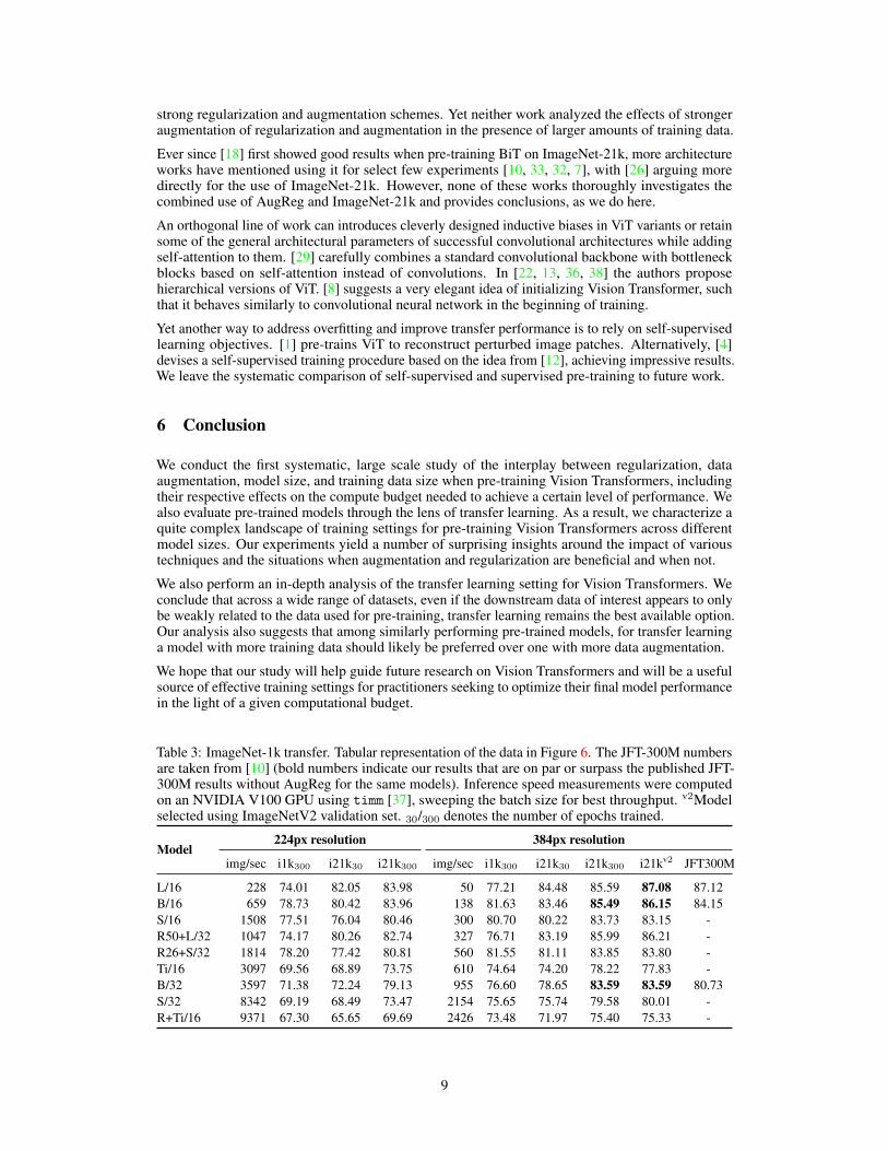
Figure 6: Imagenet transfer. Left: For every architecture and upstream dataset, we selected the bestmodel by upstream validation accuracy. Main ViT-S,B,L models are connected with a solid line tohighlight the trend, with the exception of ViT-L models pre-trained on i1k, where the trend breaksdown. The same data is also shown in Table 3. Right: Focusing on small models, it is evident thatusing a larger patch-size (/32) significantly outperforms making the model thinner (Ti).

is beneficial to adapt all models. Thus, we conclude that selecting a single pre-trained model based onthe upstream score is a cost-effective practical strategy and also use it throughout our paper. However,we also stress that if extra compute resources are available, then in certain cases one can furtherimprove adaptation performance by fine-tuning additional pre-trained models.

A note on validation data for the ImageNet-1k dataset. While performing the above analysis,we observed a subtle, but severe issue with models pre-trained on ImageNet-21k and transferredto ImageNet-1k dataset. The validation score for these models (especially for large models) is notwell correlated with observed test performance, see Figure 5 (left). This is due to the fact thatImageNet-21k data contains ImageNet-1k training data and we use a “minival“ split from the trainingdata for evaluation (see Section 3.1). As a result, large models on long training schedules memorizethe data from the training set, which biases the evaluation metric computed in the “minival“ evaluationset. To address this issue and enable fair hyper-parameter selection, we instead use the independentlycollected ImageNetV2 data [25] as the validation split for transferring to ImageNet-1k. As shown inFigure 5 (right), this resolves the issue. We did not observe similar issues for the other datasets. Werecommend that researchers transferring ImageNet-21k models to ImageNet-1k follow this strategy.

4.6 Prefer increasing patch-size to shrinking model-size

One unexpected outcome of our study is that we trained several models that are roughly equal interms of inference throughput, but vary widely in terms of their quality. Specifically, Figure 6 (right)shows that models containing the “Tiny” variants perform significantly worse than the similarly fastlarger models with “/32” patch-size. For a given resolution, the patch-size influences the amount oftokens on which self-attention is performed and, thus, is a contributor to model capacity which is notreflected by parameter count. Parameter count is reflective neither of speed, nor of capacity.

5 Related work

The scope of this paper is limited to studying pre-training and transfer learning of Vision Transformermodels and there already are a number of studies considering similar questions for convolutionalneural networks [19, 18]. Here we hence focus on related work involving ViT models.

As first proposed in [10], ViT achieved competitive performance only when trained on comparativelylarge amounts of training data, with state-of-the-art transfer results using the ImageNet-21k andJFT-300M datasets, with roughly 13M and 300M images, respectively. In stark contrast, [34]focused on tackling overfitting of ViT when training from scratch on ImageNet-1k by designing

8

strong regularization and augmentation schemes. Yet neither work analyzed the effects of strongeraugmentation of regularization and augmentation in the presence of larger amounts of training data.

Ever since [18] first showed good results when pre-training BiT on ImageNet-21k, more architectureworks have mentioned using it for select few experiments [10, 33, 32, 7], with [26] arguing moredirectly for the use of ImageNet-21k. However, none of these works thoroughly investigates thecombined use of AugReg and ImageNet-21k and provides conclusions, as we do here.

An orthogonal line of work can introduces cleverly designed inductive biases in ViT variants or retainsome of the general architectural parameters of successful convolutional architectures while addingself-attention to them. [29] carefully combines a standard convolutional backbone with bottleneckblocks based on self-attention instead of convolutions. In [22, 13, 36, 38] the authors proposehierarchical versions of ViT. [8] suggests a very elegant idea of initializing Vision Transformer, suchthat it behaves similarly to convolutional neural network in the beginning of training.

Yet another way to address overfitting and improve transfer performance is to rely on self-supervisedlearning objectives. [1] pre-trains ViT to reconstruct perturbed image patches. Alternatively, [4]devises a self-supervised training procedure based on the idea from [12], achieving impressive results.We leave the systematic comparison of self-supervised and supervised pre-training to future work.

6 Conclusion

We conduct the first systematic, large scale study of the interplay between regularization, dataaugmentation, model size, and training data size when pre-training Vision Transformers, includingtheir respective effects on the compute budget needed to achieve a certain level of performance. Wealso evaluate pre-trained models through the lens of transfer learning. As a result, we characterize aquite complex landscape of training settings for pre-training Vision Transformers across differentmodel sizes. Our experiments yield a number of surprising insights around the impact of varioustechniques and the situations when augmentation and regularization are beneficial and when not.

We also perform an in-depth analysis of the transfer learning setting for Vision Transformers. Weconclude that across a wide range of datasets, even if the downstream data of interest appears to onlybe weakly related to the data used for pre-training, transfer learning remains the best available option.Our analysis also suggests that among similarly performing pre-trained models, for transfer learninga model with more training data should likely be preferred over one with more data augmentation.

We hope that our study will help guide future research on Vision Transformers and will be a usefulsource of effective training settings for practitioners seeking to optimize their final model performancein the light of a given computational budget.

Table 3: ImageNet-1k transfer. Tabular representation of the data in Figure 6. The JFT-300M numbersare taken from [10] (bold numbers indicate our results that are on par or surpass the published JFT-300M results without AugReg for the same models). Inference speed measurements were computedon an NVIDIA V100 GPU using timm [37], sweeping the batch size for best throughput. v2Modelselected using ImageNetV2 validation set. 30/300 denotes the number of epochs trained.

Model224px resolution 384px resolution

img/sec i1k300 i21k30 i21k300 img/sec i1k300 i21k30 i21k300 i21kv2 JFT300M

L/16 228 74.01 82.05 83.98 50 77.21 84.48 85.59 87.08 87.12B/16 659 78.73 80.42 83.96 138 81.63 83.46 85.49 86.15 84.15S/16 1508 77.51 76.04 80.46 300 80.70 80.22 83.73 83.15 -R50+L/32 1047 74.17 80.26 82.74 327 76.71 83.19 85.99 86.21 -R26+S/32 1814 78.20 77.42 80.81 560 81.55 81.11 83.85 83.80 -Ti/16 3097 69.56 68.89 73.75 610 74.64 74.20 78.22 77.83 -B/32 3597 71.38 72.24 79.13 955 76.60 78.65 83.59 83.59 80.73S/32 8342 69.19 68.49 73.47 2154 75.65 75.74 79.58 80.01 -R+Ti/16 9371 67.30 65.65 69.69 2426 73.48 71.97 75.40 75.33 -

9

Acknowledgements We thank Alexey Dosovitskiy, Neil Houlsby, and Ting Chen for many insight-ful feedbacks; the Google Brain team at large for providing a supportive research environment.

References

[1] Sara Atito, Muhammad Awais, and Josef Kittler. Sit: Self-supervised vision transformer. arXiv preprintarXiv:2104.03602, 2021. 9

[2] Irwan Bello, William Fedus, Xianzhi Du, Ekin D. Cubuk, Aravind Srinivas, Tsung-Yi Lin, JonathonShlens, and Barret Zoph. Revisiting resnets: Improved training and scaling strategies. arXiv preprintarXiv:2103.07579, 2021. 4

[3] James Bradbury, Roy Frostig, Peter Hawkins, Matthew James Johnson, Chris Leary, Dougal Maclau-rin, George Necula, Adam Paszke, Jake VanderPlas, Skye Wanderman-Milne, and Qiao Zhang. JAX:composable transformations of Python+NumPy programs, 2018. 3

[4] Mathilde Caron, Hugo Touvron, Ishan Misra, Hervé Jégou, Julien Mairal, Piotr Bojanowski, and ArmandJoulin. Emerging properties in self-supervised vision transformers. arXiv preprint arXiv:2104.14294,2021. 9

[5] Gong Cheng, Junwei Han, and Xiaoqiang Lu. Remote sensing image scene classification: Benchmark andstate of the art. Proceedings of the IEEE, 105(10):1865–1883, 2017. 3

[6] Ekin D. Cubuk, Barret Zoph, Jonathon Shlens, and Quoc V. Le. RandAugment: Practical automated dataaugmentation with a reduced search space. In CVPR Workshops, 2020. 4

[7] Zihang Dai, Hanxiao Liu, Quoc V. Le, and Mingxing Tan. Coatnet: Marrying convolution and attentionfor all data sizes, 2021. 9

[8] Stéphane d’Ascoli, Hugo Touvron, Matthew Leavitt, Ari Morcos, Giulio Biroli, and Levent Sagun. Convit:Improving vision transformers with soft convolutional inductive biases. arXiv preprint arXiv:2103.10697,2021. 9

[9] J. Deng, W. Dong, R. Socher, L. Li, Kai Li, and Li Fei-Fei. Imagenet: A large-scale hierarchical imagedatabase. In CVPR, 2009. 3

[10] Alexey Dosovitskiy, Lucas Beyer, Alexander Kolesnikov, Dirk Weissenborn, Xiaohua Zhai, ThomasUnterthiner, Mostafa Dehghani, Matthias Minderer, Georg Heigold, Sylvain Gelly, Jakob Uszkoreit, andNeil Houlsby. An image is worth 16x16 words: Transformers for image recognition at scale. arXiv preprintarXiv:2010.11929, 2020. 1, 3, 4, 5, 8, 9

[11] A Geiger, P Lenz, C Stiller, and R Urtasun. Vision meets robotics: The kitti dataset. The InternationalJournal of Robotics Research, 32(11):1231–1237, 2013. 3

[12] Jean-Bastien Grill, Florian Strub, Florent Altché, Corentin Tallec, Pierre H Richemond, Elena Buchatskaya,Carl Doersch, Bernardo Avila Pires, Zhaohan Daniel Guo, Mohammad Gheshlaghi Azar, et al. Bootstrapyour own latent: A new approach to self-supervised learning. arXiv preprint arXiv:2006.07733, 2020. 9

[13] Kai Han, An Xiao, Enhua Wu, Jianyuan Guo, Chunjing Xu, and Yunhe Wang. Transformer in transformer.arXiv preprint arXiv:2103.00112, 2021. 9

[14] Kaiming He, Xiangyu Zhang, Shaoqing Ren, and Jian Sun. Deep residual learning for image recognition.In CVPR, 2016. 1, 4

[15] Jonathan Heek, Anselm Levskaya, Avital Oliver, Marvin Ritter, Bertrand Rondepierre, Andreas Steiner,and Marc van Zee. Flax: A neural network library and ecosystem for JAX, 2020. 3

[16] Gao Huang, Yu Sun, Zhuang Liu, Daniel Sedra, and Kilian Q Weinberger. Deep networks with stochasticdepth. In ECCV, 2016. 4

[17] Diederik P. Kingma and Jimmy Ba. Adam: A method for stochastic optimization. In ICLR, 2015. 4[18] Alexander Kolesnikov, Lucas Beyer, Xiaohua Zhai, Joan Puigcerver, Jessica Yung, Sylvain Gelly, and Neil

Houlsby. Big transfer (BiT): General visual representation learning. In ECCV, 2020. 3, 8, 9[19] Simon Kornblith, Jonathon Shlens, and Quoc V Le. Do better imagenet models transfer better? In CVPR,

2019. 8[20] Alex Krizhevsky. Learning multiple layers of features from tiny images. Technical report, 2009. 3[21] Alex Krizhevsky, Ilya Sutskever, and Geoffrey E. Hinton. ImageNet classification with deep convolutional

neural networks. In NeurIPS, 2012. 2[22] Ze Liu, Yutong Lin, Yue Cao, Han Hu, Yixuan Wei, Zheng Zhang, Stephen Lin, and Baining Guo. Swin

transformer: Hierarchical vision transformer using shifted windows. arXiv preprint arXiv:2103.14030,2021. 9

[23] Ilya Loshchilov and Frank Hutter. Decoupled weight decay regularization. In International Conference onLearning Representations, 2019. 4, 12

[24] Omkar M. Parkhi, Andrea Vedaldi, Andrew Zisserman, and C. V. Jawahar. Cats and dogs. In CVPR, 2012.3

[25] Benjamin Recht, Rebecca Roelofs, Ludwig Schmidt, and Vaishaal Shankar. Do imagenet classifiersgeneralize to imagenet? 2019. 3, 8

[26] Tal Ridnik, Emanuel Ben-Baruch, Asaf Noy, and Lihi Zelnik-Manor. Imagenet-21k pretraining for themasses. arXiv preprint arXiv:2104.10972, 2021. 3, 9

[27] Olga Russakovsky, Jia Deng, Hao Su, Jonathan Krause, Sanjeev Satheesh, Sean Ma, Zhiheng Huang,Andrej Karpathy, Aditya Khosla, Michael Bernstein, et al. Imagenet large scale visual recognition challenge.IIJCV, 2015. 5

10

[28] Ali Sharif Razavian, Hossein Azizpour, Josephine Sullivan, and Stefan Carlsson. Cnn features off-the-shelf:An astounding baseline for recognition. In Proceedings of the IEEE Conference on Computer Vision andPattern Recognition (CVPR) Workshops, June 2014. 2

[29] Aravind Srinivas, Tsung-Yi Lin, Niki Parmar, Jonathon Shlens, Pieter Abbeel, and Ashish Vaswani.Bottleneck transformers for visual recognition. arXiv preprint arXiv:2101.11605, 2021. 9

[30] Chen Sun, Abhinav Shrivastava, Saurabh Singh, and Abhinav Gupta. Revisiting unreasonable effectivenessof data in deep learning era. In Proceedings of the IEEE international conference on computer vision,pages 843–852, 2017. 5

[31] C. Szegedy, W. Liu, Y. Jia, P. Sermanet, S. Reed, D. Anguelov, D. Erhan, V. Vanhoucke, and A. Rabinovich.Going deeper with convolutions. In CVPR, 2015. 4

[32] Mingxing Tan and Quoc V. Le. Efficientnetv2: Smaller models and faster training. CoRR, abs/2104.00298,2021. 9

[33] Ilya O. Tolstikhin, Neil Houlsby, Alexander Kolesnikov, Lucas Beyer, Xiaohua Zhai, Thomas Unterthiner,Jessica Yung, Andreas Steiner, Daniel Keysers, Jakob Uszkoreit, Mario Lucic, and Alexey Dosovitskiy.Mlp-mixer: An all-mlp architecture for vision. CoRR, abs/2105.01601, 2021. 9

[34] Hugo Touvron, Matthieu Cord, Matthijs Douze, Francisco Massa, Alexandre Sablayrolles, and HervéJégou. Training data-efficient image transformers & distillation through attention. arXiv preprintarXiv:2012.12877, 2020. 1, 3, 4, 8

[35] Hugo Touvron, Andrea Vedaldi, Matthijs Douze, and Herve Jegou. Fixing the train-test resolutiondiscrepancy. In NeurIPS, 2019. 4

[36] Wenhai Wang, Enze Xie, Xiang Li, Deng-Ping Fan, Kaitao Song, Ding Liang, Tong Lu, Ping Luo, andLing Shao. Pyramid vision transformer: A versatile backbone for dense prediction without convolutions.arXiv preprint arXiv:2102.12122, 2021. 9

[37] Ross Wightman. Pytorch image models (timm): Vit training details. https://github.com/rwightman/pytorch-image-models/issues/252#issuecomment-713838112, 2013. 3, 9

[38] Haiping Wu, Bin Xiao, Noel Codella, Mengchen Liu, Xiyang Dai, Lu Yuan, and Lei Zhang. Cvt:Introducing convolutions to vision transformers. arXiv preprint arXiv:2103.15808, 2021. 9

[39] Qizhe Xie, Zihang Dai, Eduard Hovy, Thang Luong, and Quoc Le. Unsupervised data augmentation forconsistency training. In H. Larochelle, M. Ranzato, R. Hadsell, M. F. Balcan, and H. Lin, editors, Advancesin Neural Information Processing Systems, 2020. 5

[40] Xiaohua Zhai, Joan Puigcerver, Alexander Kolesnikov, Pierre Ruyssen, Carlos Riquelme, Mario Lucic,Josip Djolonga, Andre Susano Pinto, Maxim Neumann, Alexey Dosovitskiy, Lucas Beyer, Olivier Bachem,Michael Tschannen, Marcin Michalski, Olivier Bousquet, Sylvain Gelly, and Neil Houlsby. A large-scalestudy of representation learning with the visual task adaptation benchmark, 2020. 2, 3, 6, 13

[41] Hongyi Zhang, Moustapha Cisse, Yann N Dauphin, and David Lopez-Paz. mixup: Beyond empirical riskminimization. In ICLR, 2018. 4

11

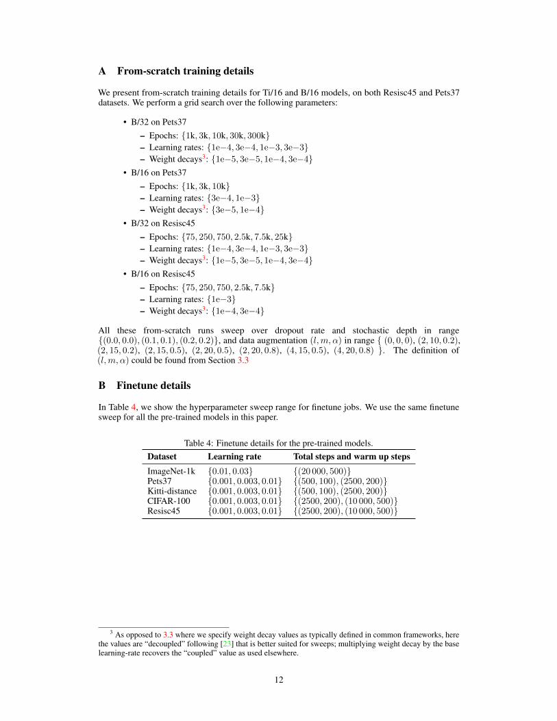
A From-scratch training details

We present from-scratch training details for Ti/16 and B/16 models, on both Resisc45 and Pets37datasets. We perform a grid search over the following parameters:

• B/32 on Pets37– Epochs: {1k, 3k, 10k, 30k, 300k}– Learning rates: {1e−4, 3e−4, 1e−3, 3e−3}– Weight decays3: {1e−5, 3e−5, 1e−4, 3e−4}

• B/16 on Pets37– Epochs: {1k, 3k, 10k}– Learning rates: {3e−4, 1e−3}– Weight decays3: {3e−5, 1e−4}

• B/32 on Resisc45– Epochs: {75, 250, 750, 2.5k, 7.5k, 25k}– Learning rates: {1e−4, 3e−4, 1e−3, 3e−3}– Weight decays3: {1e−5, 3e−5, 1e−4, 3e−4}

• B/16 on Resisc45– Epochs: {75, 250, 750, 2.5k, 7.5k}– Learning rates: {1e−3}– Weight decays3: {1e−4, 3e−4}

All these from-scratch runs sweep over dropout rate and stochastic depth in range{(0.0, 0.0), (0.1, 0.1), (0.2, 0.2)}, and data augmentation (l,m, α) in range { (0, 0, 0), (2, 10, 0.2),(2, 15, 0.2), (2, 15, 0.5), (2, 20, 0.5), (2, 20, 0.8), (4, 15, 0.5), (4, 20, 0.8) }. The definition of(l,m, α) could be found from Section 3.3

B Finetune details

In Table 4, we show the hyperparameter sweep range for finetune jobs. We use the same finetunesweep for all the pre-trained models in this paper.

Table 4: Finetune details for the pre-trained models.Dataset Learning rate Total steps and warm up stepsImageNet-1k {0.01, 0.03} {(20 000, 500)}Pets37 {0.001, 0.003, 0.01} {(500, 100), (2500, 200)}Kitti-distance {0.001, 0.003, 0.01} {(500, 100), (2500, 200)}CIFAR-100 {0.001, 0.003, 0.01} {(2500, 200), (10 000, 500)}Resisc45 {0.001, 0.003, 0.01} {(2500, 200), (10 000, 500)}

3 As opposed to 3.3 where we specify weight decay values as typically defined in common frameworks, herethe values are “decoupled” following [23] that is better suited for sweeps; multiplying weight decay by the baselearning-rate recovers the “coupled” value as used elsewhere.

12

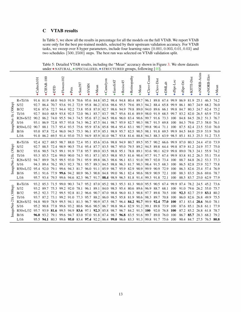
C VTAB results

In Table 5, we show all the results in percentage for all the models on the full VTAB. We report VTABscore only for the best pre-trained models, selected by their upstream validation accuracy. For VTABtasks, we sweep over 8 hyper parameters, include four learning rates {0.001, 0.003, 0.01, 0.03} andtwo schedules {500, 2500} steps. The best run was selected on VTAB validation split.

Table 5: Detailed VTAB results, including the “Mean” accuracy shown in Figure 3. We show datasetsunder NATURAL, SPECIALIZED, STRUCTURED groups, following [40].

Cal

tech

101

CIF

AR

-100

DT

D

Flow

ers1

02

Pets

Sun3

97

SVH

N

Mea

n

Cam

elyo

n

Eur

oSA

T

Res

isc4

5

Ret

inop

athy

Mea

n

Cle

vr-C

ount

Cle

vr-D

ist

DM

Lab

dSpr

-Loc

dSpr

-Ori

KIT

TI-

Dis

t

sNO

RB

-Azi

m

sNO

RB

-Ele

v

Mea

n

Imag

eNet

-1k

(300

ep) R+Ti/16 91.6 81.9 68.0 94.0 91.9 70.6 95.6 84.8 85.2 98.4 94.8 80.4 89.7 96.1 89.8 67.4 99.9 86.9 81.9 25.1 46.3 74.2

S/32 92.7 86.4 70.7 93.6 91.2 72.9 95.8 86.2 83.6 98.6 95.5 79.6 89.3 94.2 88.4 65.8 99.9 86.1 80.7 24.9 68.2 76.0B/32 92.6 87.6 72.7 94.4 92.2 73.8 95.8 87.0 82.7 98.6 94.9 79.8 89.0 94.0 89.6 66.1 99.8 84.7 80.3 24.7 62.4 75.2Ti/16 92.7 84.0 68.9 93.8 92.5 72.0 96.1 85.7 83.7 98.7 95.6 81.6 89.9 98.0 91.9 68.5 99.7 83.2 82.0 26.5 65.9 77.0R26+S/32 90.2 86.2 74.0 95.5 94.3 74.5 95.6 87.2 84.5 98.6 96.0 83.4 90.6 99.7 91.6 73.3 100 84.8 84.5 28.2 51.3 76.7S/16 93.1 86.9 72.8 95.7 93.8 74.3 96.2 87.5 84.1 98.7 95.9 82.7 90.3 98.7 91.5 69.8 100 84.3 79.6 27.3 58.0 76.1R50+L/32 90.7 88.1 73.7 95.4 93.5 75.6 95.9 87.6 85.8 98.4 95.4 83.1 90.7 99.8 90.4 71.1 100 87.5 82.4 23.5 53.0 76.0B/16 93.0 87.8 72.4 96.0 94.5 75.3 96.1 87.9 85.1 98.9 95.7 82.5 90.5 98.1 91.8 69.5 99.9 84.5 84.0 25.9 53.9 76.0L/16 91.0 86.2 69.5 91.4 93.0 75.3 94.9 85.9 81.0 98.7 93.8 81.6 88.8 94.3 88.3 63.9 98.5 85.1 81.3 25.3 51.2 73.5

Imag

eNet

-21k

(30e

p)

R+Ti/16 92.4 82.7 69.5 98.7 88.0 72.4 95.1 85.6 83.6 98.8 94.9 80.7 89.5 95.7 90.2 66.6 99.9 87.0 80.3 24.4 47.0 73.9S/32 92.7 88.5 72.4 98.9 90.5 75.4 95.4 87.7 83.5 98.7 95.0 79.5 89.2 94.5 89.8 64.4 99.8 87.9 81.2 24.9 57.7 75.0B/32 93.6 90.5 74.5 99.1 91.9 77.8 95.7 89.0 83.5 98.8 95.1 78.8 89.1 93.6 90.1 62.9 99.8 89.0 78.3 24.1 55.9 74.2Ti/16 93.3 85.5 72.6 99.0 90.0 74.3 95.1 87.1 85.5 98.8 95.5 81.6 90.4 97.7 91.7 67.4 99.9 83.8 81.2 26.3 55.1 75.4R26+S/32 94.7 89.9 76.5 99.5 93.0 79.1 95.9 89.8 86.3 98.6 96.1 83.1 91.0 99.7 92.0 73.4 100 88.7 84.8 26.2 53.3 77.3S/16 94.3 89.4 76.2 99.3 92.3 78.1 95.7 89.3 84.5 98.8 96.3 81.7 90.3 98.4 91.5 68.3 100 86.5 82.8 25.9 52.7 75.8R50+L/32 95.4 92.0 79.1 99.6 94.3 81.7 96.0 91.1 85.9 98.7 95.9 82.9 90.9 99.9 90.9 72.9 100 86.3 82.6 25.4 57.4 76.9B/16 95.1 91.6 77.9 99.6 94.2 80.9 96.3 90.8 84.8 99.0 96.1 82.4 90.6 98.9 90.9 72.1 100 88.3 83.5 26.6 69.6 78.7L/16 95.7 93.4 79.5 99.6 94.6 82.3 96.7 91.7 88.4 98.9 96.5 81.8 91.4 99.3 91.8 72.1 100 88.5 83.7 25.0 62.9 77.9

Imag

eNet

-21k

(300

ep) R+Ti/16 93.2 85.3 71.5 99.0 90.3 74.7 95.2 87.0 85.2 98.3 95.3 81.3 90.0 95.5 90.5 67.4 99.9 87.4 78.2 24.5 45.2 73.6

S/32 93.2 89.7 75.3 99.2 92.0 78.1 96.1 89.1 84.0 98.5 95.4 80.6 89.6 96.9 88.7 68.1 100 91.0 79.6 26.2 55.0 75.7B/32 95.2 92.3 77.2 99.5 92.8 81.2 96.6 90.7 87.0 98.8 96.0 81.3 90.8 97.7 89.8 70.5 100 92.3 82.7 25.9 83.1 80.2Ti/16 93.7 87.2 73.1 99.2 91.0 77.3 95.7 88.2 86.0 98.5 95.8 81.9 90.6 98.3 89.7 70.8 100 86.0 82.6 26.8 49.9 75.5R26+S/32 94.8 90.9 78.9 99.5 94.1 81.3 96.7 90.9 87.5 98.7 96.4 84.2 91.7 99.9 92.4 77.0 100 87.1 83.4 28.6 56.0 78.1S/16 95.2 90.8 77.8 99.6 93.2 80.6 96.6 90.5 86.7 98.8 96.4 82.9 91.2 99.1 89.8 73.9 100 87.6 85.1 26.8 61.1 77.9R50+L/32 95.7 93.9 81.6 99.5 94.9 83.6 97.1 92.3 85.8 98.7 96.7 84.2 91.3 100 92.0 76.8 100 87.2 85.2 26.8 61.8 78.7B/16 96.0 93.2 79.1 99.6 94.7 83.0 97.0 91.8 87.4 98.7 96.8 83.5 91.6 99.7 89.0 76.0 100 86.7 85.7 28.3 68.2 79.2L/16 95.5 94.1 80.3 99.6 95.0 83.4 97.4 92.2 86.4 99.0 96.6 83.3 91.3 99.8 91.7 75.6 100 90.4 84.7 27.5 76.5 80.8

13

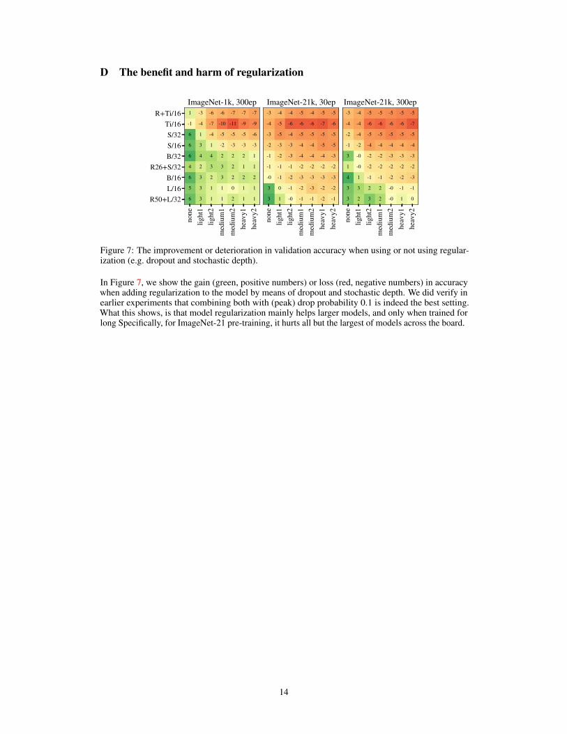
D The benefit and harm of regularization

none

light

1lig

ht2

med

ium

1m

ediu

m2

heav

y1he

avy2

R+Ti/16Ti/16S/32S/16B/32

R26+S/32B/16L/16

R50+L/32

1 -3 -6 -6 -7 -7 -7

-1 -4 -7 -10 -11 -9 -9

6 1 -4 -5 -5 -5 -6

6 3 1 -2 -3 -3 -3

6 4 4 2 2 2 1

4 2 3 3 2 1 1

6 3 2 3 2 2 2

5 3 1 1 0 1 1

6 3 1 1 2 1 1

ImageNet-1k, 300ep

none

light

1lig

ht2

med

ium

1m

ediu

m2

heav

y1he

avy2

-3 -4 -4 -5 -4 -5 -5

-4 -5 -6 -6 -6 -7 -6

-3 -5 -4 -5 -5 -5 -5

-2 -3 -3 -4 -4 -5 -5

-1 -2 -3 -4 -4 -4 -3

-1 -1 -1 -2 -2 -2 -2

-0 -1 -2 -3 -3 -3 -3

3 0 -1 -2 -3 -2 -2

3 1 -0 -1 -1 -2 -1

ImageNet-21k, 30ep

none

light

1lig

ht2

med

ium

1m

ediu

m2

heav

y1he

avy2

-3 -4 -5 -5 -5 -5 -5

-4 -4 -6 -6 -6 -6 -7

-2 -4 -5 -5 -5 -5 -5

-1 -2 -4 -4 -4 -4 -4

3 -0 -2 -2 -3 -3 -3

1 -0 -2 -2 -2 -2 -2

4 1 -1 -1 -2 -2 -3

3 3 2 2 -0 -1 -1

3 2 3 2 -0 1 0

ImageNet-21k, 300ep

Figure 7: The improvement or deterioration in validation accuracy when using or not using regular-ization (e.g. dropout and stochastic depth).

In Figure 7, we show the gain (green, positive numbers) or loss (red, negative numbers) in accuracywhen adding regularization to the model by means of dropout and stochastic depth. We did verify inearlier experiments that combining both with (peak) drop probability 0.1 is indeed the best setting.What this shows, is that model regularization mainly helps larger models, and only when trained forlong Specifically, for ImageNet-21 pre-training, it hurts all but the largest of models across the board.

14