How to Specify Crystal Filters

C.W. (bill) Pond and David Kemper

Abstract: A way to specify a crystal filter is discussed and an example, showing sample specifications is presented. The advantages and disadvantages and the factors that are unique to crystal filters are discussed along with the factors that influence the cost. Background information showing the range where crystal filters can be manufactured is specified along with some common definitions and helpful formulas.

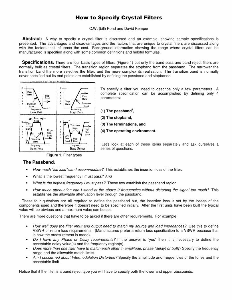
Specifications: There are four basic types of filters (Figure 1) but only the band pass and band reject filters are normally built as crystal filters. The transition region separates the stopband from the passband. The narrower the transition band the more selective the filter, and the more complex its realization. The transition band is normally never specified but its end points are established by defining the passband and stopbands.

To specify a filter you need to describe only a few parameters. A complete specification can be accomplished by defining only 4 parameters:

(1) The passband1,

(2) The stopband,

(3) The terminations, and

(4) The operating environment.

Let’s look at each of these items separately and ask ourselves a series of questions.

Figure 1. Filter types

The Passband:

• How much “flat loss” can I accommodate? This establishes the insertion loss of the filter.

• What is the lowest frequency I must pass? And

What is the highest frequency I must pass? These two establish the passband region.

• How much attenuation can I stand at the above 2 frequencies without distorting the signal too much? This establishes the allowable attenuation level through the passband.

These four questions are all required to define the passband but, the insertion loss is set by the losses of the components used and therefore it doesn’t need to be specified initially. After the first units have been built the typical value will be obvious and a maximum value can be set.

There are more questions that have to be asked if there are other requirements. For example:

• How well does the filter input and output need to match my source and load impedances? Use this to define VSWR or return loss requirements. (Manufactures prefer a return loss specification to a VSWR because that is how the measurement is made).

• Do I have any Phase or Delay requirements? If the answer is “yes” then it is necessary to define the acceptable delay value(s) and the frequency region(s).

• Does more than one filter have to match each other in amplitude, phase (delay) or both? Specify the frequency range and the allowable match limits.

• Am I concerned about Intermodulation Distortion? Specify the amplitude and frequencies of the tones and the acceptable limit.

Notice that if the filter is a band reject type you will have to specify both the lower and upper passbands.

The Stopband:

• What is the lowest frequency I need rejected and how much attenuation is required? This sets the limit on the lower stopband and it could be all the way down to DC.

• What are the frequency and attenuation values required at the end of the lower transition band?

• Repeat the same two questions for the upper stopband region.

The stopband could have several ranges where different attenuation values are required. Each of these regions must be defined from their lowest to highest frequencies and the attenuation required.

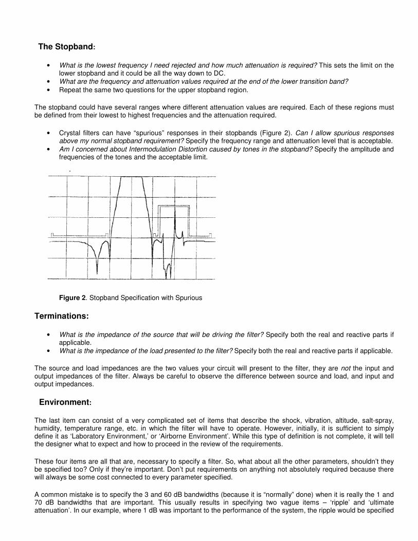
• Crystal filters can have “spurious” responses in their stopbands (Figure 2). Can I allow spurious responses above my normal stopband requirement? Specify the frequency range and attenuation level that is acceptable.

• Am I concerned about Intermodulation Distortion caused by tones in the stopband? Specify the amplitude and frequencies of the tones and the acceptable limit.

Figure 2. Stopband Specification with Spurious

Terminations:

• What is the impedance of the source that will be driving the filter? Specify both the real and reactive parts if applicable.

• What is the impedance of the load presented to the filter? Specify both the real and reactive parts if applicable.

The source and load impedances are the two values your circuit will present to the filter, they are not the input and output impedances of the filter. Always be careful to observe the difference between source and load, and input and output impedances.

Environment:

The last item can consist of a very complicated set of items that describe the shock, vibration, altitude, salt-spray, humidity, temperature range, etc. in which the filter will have to operate. However, initially, it is sufficient to simply define it as ‘Laboratory Environment,’ or ‘Airborne Environment’. While this type of definition is not complete, it will tell the designer what to expect and how to proceed in the review of the requirements.

These four items are all that are, necessary to specify a filter. So, what about all the other parameters, shouldn’t they be specified too? Only if they’re important. Don’t put requirements on anything not absolutely required because there will always be some cost connected to every parameter specified.

A common mistake is to specify the 3 and 60 dB bandwidths (because it is “normally” done) when it is really the 1 and 70 dB bandwidths that are important. This usually results in specifying two vague items – ‘ripple’ and ‘ultimate attenuation’. In our example, where 1 dB was important to the performance of the system, the ripple would be specified

to be 1 dB max. This seems alright but the difficulty comes from the definition of ‘ripple’. Ripple is normally defined to be the difference between the highest peak and lowest valley in the passband. This works when there are clearly defined peaks and valleys, but it fails when there are inflection points or the overall response is very rounded (like a bald-headed man). Thus, if it is really necessary to have a passband with 1 dB of flatness then it is necessary to specify it that way. Ripple need not be specified at all, because any dip below 1 dB would fail the bandwidth requirement.

The second problem specification is ‘ultimate attenuation’. Again from our example, the 60 dB bandwidth was specified (because grandfather did it that way) and the ‘ultimate attenuation’ specified to be 70dB. The problem with this is that there is no frequency range associated with it. The filter manufacture is free to select the frequency(s) where 70 dB is attained.

The clearest and cleanest way to write a specification is to define exactly what your system requirements are. Don’t specify something you don’t need and don’t specify something because it is “normally” done that way.

Example 1. A Spectral Clean-Up Filter:

You have a 5 MHz master oscillator and used to generate a spectrum of frequencies. Write a specification for a filter which will select the 90 MHz ‘tone’ from that spectrum. The center frequency of the filter (Fo) will be, by definition, 90 MHz.

• How much “flat loss” can I accommodate? This value is not critical since amplifiers will be necessary anyway so initially specify it as 10 dB and allow the vendor to establish the value used in production.

• What is the lowest frequency I must pass? The stability of the master oscillator is �.01 ppM so the filter must be designed to pass this under all operating condition. Select it to be Fo-10 Hz.

• What is the highest frequency I must pass? Select it to be Fo+ 10 Hz. • How much attenuation can I stand at the above two frequencies without distorting the signal too much? I don’t

want the gain through this circuit to change more than �2 dB and so budget 1 dB to the filter. Thus the 1 dB bandwidth will be Fo�10 Hz min.

• What is the lowest frequency I need rejected and how much attenuation is required? This will be the lowest frequency where any signal resides, which is 5 MHz. Select the minimum attenuation level to be 40 dB.

• What are the frequency and attenuation values required at the end of the lower transition band? This is the closest frequency on the low side, - 85MHz. Select the minimum attenuation level to be 40 dB.

• What are the frequency and attenuation values required at the end of the upper transition band? This is the closest frequency on the high side, -95 MHz. Select the minimum attenuation level to be 40 dB.

• What is the highest frequency I need rejected and how much attenuation is required? This will be the highest frequency before natural roll-off occurs. Chose it to be 200 MHz. Select the minimum attenuation level to be 40 dB.

• Can I allow spurious responses above my normal stopband requirement? No, 40 dB overall attenuation must be maintained.

• What is the impedance of the source that will be driving the filter? Use 50� resistive with negligible reactive source.

• What is the impedance of the load presented to the filter? Use 50� resistive with negligible reactive load.

• The unit will operate in an ‘Airborne Environment’ and the enclosure is “open” except that it must be no higher than 0.55” and suitable for surface mounting.

Summary:

Center Frequency (Fo) 90.00MHz

1 dB Bandwidth Fo�10.0 Hz Min

40 dB Bandwidth Fo�5.0 MHz Max

Lower 40 dB 5.0 to 85.0 MHz

Upper 40 dB attenuation 95.0 to 200 MHz

Source and Load impedance 50.0� �5%

Enclosure TBD”LXTBD”WX0.55” H Max

Environment Airborne.

A worksheet to help in preparing a crystal filter specification is included in Appendix D.

Advantages of Crystal Filters.

Crystal resonators have very high Qs and excellent temperature and aging characteristics. These benefits are translated to the filters so that very narrow bandwidths and highly selective filters can be achieved.

The change of frequency with temperature can be as low as �20 ppM over a full military (-45 to + 85 0C) temperature

range.

The aging of narrow and intermediate band crystal filters is almost solely dependent upon the aging of the crystals themselves. Thus, after proper conditioning, it is possible for the filters to age no more than a fraction of a part-per-million per year. This makes crystal filters ideally suited for phase-matched applications.

Because of the high Q values available from the crystals (Qs of up to a million are possible with Qs of 100k being typical) very narrow and very selective filters can be made. Filters with shape factors (60/3 dB) of as low as 1.015:1 have been built. Bandwidths as narrow as 0.001% are routinely produced.

Disadvantages of Crystal Filters.

There are two basic problems associated with crystal filters: spurious responses and non-linear drive level responses.

The spurious responses are caused by, inharmonically related, modes of vibration in the crystal. They appear in the filter as narrow responses that degrade whatever band they appear in. For example, if they appear in the stopband, the attenuation is decreased (Figure 1) but if they appear in the passband they will introduce an unwanted notch. Generally, spurious responses are very narrow and don’t cause a problem unless an unwanted signal appears at their frequency. They have a minimal impact on the overall noise bandwidth. More on spurious later.

The non-linear drive level causes a series of problems. First it limits the drive level to a maximum of +10 dB with a recommended drive of –10 dBm max. Unless the crystals are carefully designed and manufactured the Q and frequency can change as a function of drive and the Q could halve as the drive level was changed from –10 to –60 dBm. Since crystal filters must operate over wide drive level ranges they should be tested over all expected drive conditions.

The non-linear drive condition is the main cause of Intermodulation distortion in crystal filters.

Operating Region.

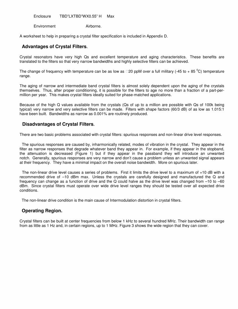
Crystal filters can be built at center frequencies from below 1 kHz to several hundred MHz. Their bandwidth can range from as little as 1 Hz and, in certain regions, up to 1 MHz. Figure 3 shows the wide region that they can cover.

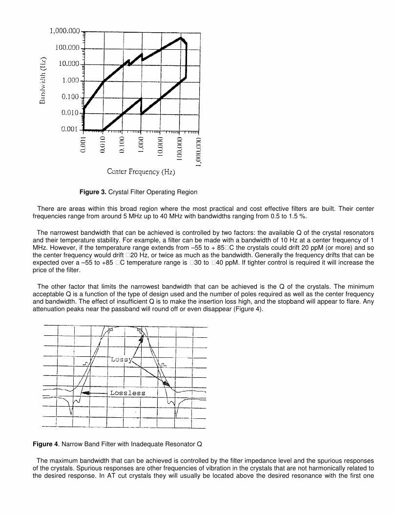
Figure 3. Crystal Filter Operating Region

There are areas within this broad region where the most practical and cost effective filters are built. Their center frequencies range from around 5 MHz up to 40 MHz with bandwidths ranging from 0.5 to 1.5 %.

The narrowest bandwidth that can be achieved is controlled by two factors: the available Q of the crystal resonators and their temperature stability. For example, a filter can be made with a bandwidth of 10 Hz at a center frequency of 1 MHz. However, if the temperature range extends from –55 to + 85�C the crystals could drift 20 ppM (or more) and so the center frequency would drift �20 Hz, or twice as much as the bandwidth. Generally the frequency drifts that can be expected over a –55 to +85 �C temperature range is �30 to �40 ppM. If tighter control is required it will increase the price of the filter.

The other factor that limits the narrowest bandwidth that can be achieved is the Q of the crystals. The minimum acceptable Q is a function of the type of design used and the number of poles required as well as the center frequency and bandwidth. The effect of insufficient Q is to make the insertion loss high, and the stopband will appear to flare. Any attenuation peaks near the passband will round off or even disappear (Figure 4).

Figure 4. Narrow Band Filter with Inadequate Resonator Q

The maximum bandwidth that can be achieved is controlled by the filter impedance level and the spurious responses of the crystals. Spurious responses are other frequencies of vibration in the crystals that are not harmonically related to the desired response. In AT cut crystals they will usually be located above the desired resonance with the first one

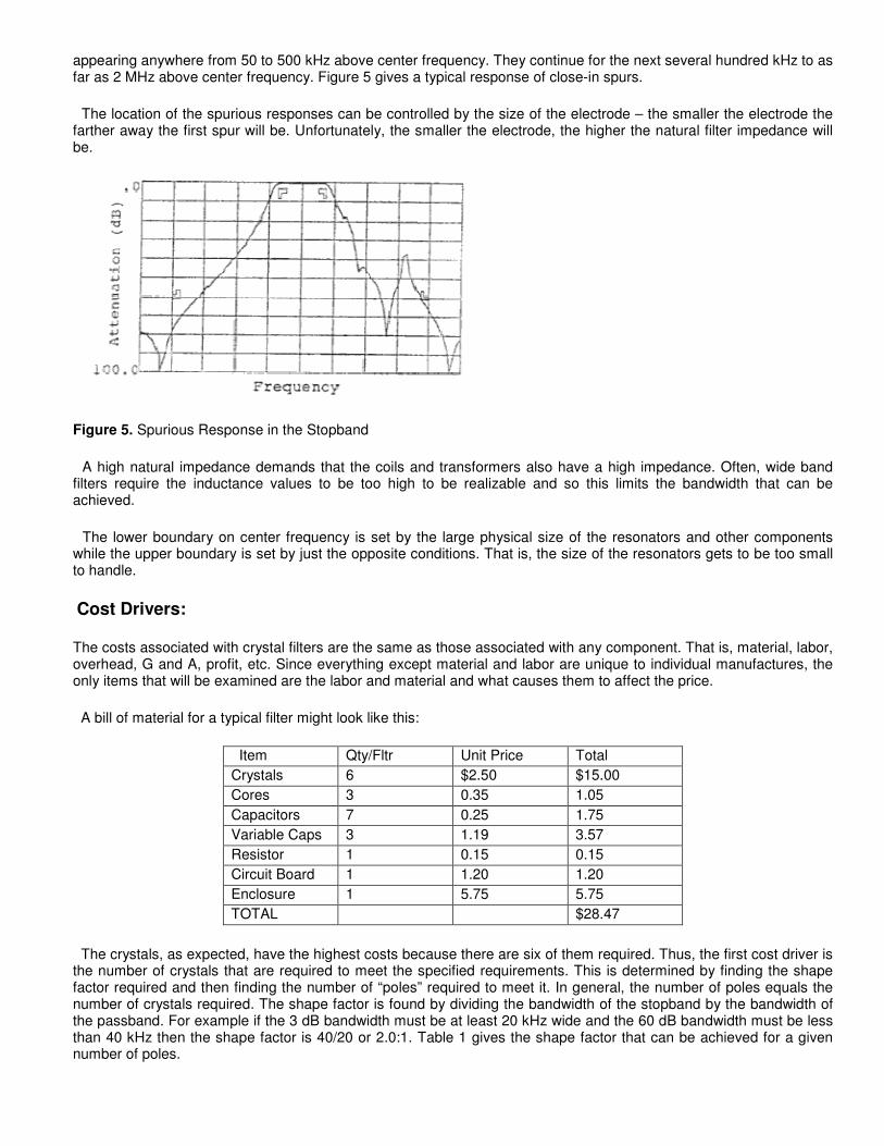
appearing anywhere from 50 to 500 kHz above center frequency. They continue for the next several hundred kHz to as far as 2 MHz above center frequency. Figure 5 gives a typical response of close-in spurs.

The location of the spurious responses can be controlled by the size of the electrode – the smaller the electrode the farther away the first spur will be. Unfortunately, the smaller the electrode, the higher the natural filter impedance will be.

Figure 5. Spurious Response in the Stopband

A high natural impedance demands that the coils and transformers also have a high impedance. Often, wide band filters require the inductance values to be too high to be realizable and so this limits the bandwidth that can be achieved.

The lower boundary on center frequency is set by the large physical size of the resonators and other components while the upper boundary is set by just the opposite conditions. That is, the size of the resonators gets to be too small to handle.

Cost Drivers:

The costs associated with crystal filters are the same as those associated with any component. That is, material, labor, overhead, G and A, profit, etc. Since everything except material and labor are unique to individual manufactures, the only items that will be examined are the labor and material and what causes them to affect the price.

A bill of material for a typical filter might look like this:

Item Qty/Fltr Unit Price Total

Crystals 6 $2.50 $15.00

Cores 3 0.35 1.05

Capacitors 7 0.25 1.75

Variable Caps 3 1.19 3.57

Resistor 1 0.15 0.15

Circuit Board 1 1.20 1.20

Enclosure 1 5.75 5.75

TOTAL $28.47

The crystals, as expected, have the highest costs because there are six of them required. Thus, the first cost driver is the number of crystals that are required to meet the specified requirements. This is determined by finding the shape factor required and then finding the number of “poles” required to meet it. In general, the number of poles equals the number of crystals required. The shape factor is found by dividing the bandwidth of the stopband by the bandwidth of the passband. For example if the 3 dB bandwidth must be at least 20 kHz wide and the 60 dB bandwidth must be less than 40 kHz then the shape factor is 40/20 or 2.0:1. Table 1 gives the shape factor that can be achieved for a given number of poles.

Table 1. Shape Factors for N Pole Monotonic Filters

No. of Poles Shape Factor

(60/3 dB) 2 30

3 10

4 5

6 2.5

7 2.1

8 1.9

10 1.5

Thus the steeper the filter, the more crystals will be required and, the higher the crystal costs. Appendix B gives the necessary equations to determine the number of poles that will be required to meet a particular shape factor.

The center frequency also influences the cost of the crystal because there are some regions where it is easier, and less costly, to manufacture crystals. Figure 6 gives a rough estimate of the relative costs of a crystal as a function of its frequency.

Figure 6. Relative Crystal Cost vs. Frequency

This graph shows only fundamental mode crystals. It indicates that the lowest cost crystals will fall from about 5 MHz up to about 35 MHz. To minimize the crystal costs reduce the number of crystals required, if possible, and select the center frequency to fall between 5 and 35 MHz.

As the bandwidth of the filter increases above 100 kHz the spurious responses can become a problem. To control them it may be necessary to (1) decrease the electrode size (which raises the impedance level). (2) parallel crystals to reduce the impedance level. Sometimes more sections must be used to control the spurious responses even though they are not needed to meet the required selectivity. Another way the bandwidth of the filter can affect the crystal costs is if the bandwidth becomes quite narrow. The crystals will have to meet vary tight Q and temperature stability requirements and their yield will drop. The best way to minimize costs due to the bandwidth associated problem is to keep the percentage bandwidth between .05 and 1.5 % and the maximum bandwidth below 200 kHz.

Either the enclosure costs or the variable capacitor costs are the second most expensive costs in the filter. In the example shown, the enclosure comes in second. The enclosure costs can vary dramatically depending on the requirements. For example, standard “drawn” cans are cheaper than fabricated enclosures and fabricated enclosures are much cheaper than machined housings. Glass feed-through terminals generally cost less than 50 cents but hermetically sealed connectors can cost $20.00 or more. Small filters that don’t need and provision for mounting (other

than their input, output and ground pins) will cost less than filters with studs. Filters requiring inserts will cost more than ones with studs, and filters that require a hole completely through the package will be even more costly. Special paint or marking inks will be even more than using the manufactured standard plated finish and marking methods.

Another factor that affects the costs is the environmental requirement. It is obvious that a “laboratory environment” will cost less than designing to operate the same filter in any other environment with the “missile environment” usually being the most costly.

The labor content can be the major cost of the filter. The factors that drive up the labor costs are such things as: difficult specifications that require a large amount of alignment time; phase and/or amplitude matching requirements; special screening and special quality requirements. It is also nearly impossible to discuss “difficult specifications” in a general sense since each filter will have its own unique tuning procedure. However, there are some general comments that can be made about phase and amplitude matching.

Phase and amplitude matching requirements force all of the filters to have identical (or nearly identical) shapes and responses. To achieve this, all the crystals and coils have to be properly tuned. This is especially difficult on very narrow or very wide bandwidths. The narrow filters demand that the crystals be precisely tuned to frequency and this increases the crystal manufacturing time and decreases the yields.

The more filters in a matched set the more difficult it is. Thus, it is cheaper to require matched pairs rather than matched trios, trios rather than quads, etc.

The largest changes in both the phase and amplitude occur near the edge of the passband. Therefore, it is more difficult to match all the way to the 3 dB point than it is to match to only 80% of the bandwidth. If it is necessary to match all the way out to the edge of the passband then it would be better is a looser specification could be used in the last 20 % of the bandwidth. For example, require a phase match of �5� over 80% of the 3 dB bandwidth and �15� over the balance.

It should be obvious that the most expensive type of matching is matching both phase and amplitude on two or more filters at the same time. This is true, of course, but it usually doesn’t raise the cost very much because filters that have been tuned to match for phase will generally have the same shapes. Unless the amplitude matching requirement is very tight most phase matched filters will also meet amplitude matched requirements as well.

Very narrow and very wide matched filters will always be the most costly. The best operating region for matched filters is from 0.05 to 1.5 %.

Summary: Crystal filters can be built with center frequencies from below 1 kHz up to several hundred MHz and bandwidths that vary from a few Hz to MHz. Very selective filters can be built with shape factors as small as 1.10:1 however, if cost is a consideration it is best to stay with shape factors of 2.0:1 or higher. The most cost effective center frequency range runs from around 5 to about 35 MHz. While the filter pass bandwidths should range from 0.05 % to 1.5 %. Filters can be built outside these limits, but these values will provide the most cost effective units.

When specifying filters it is necessary to clearly define what you want to pass and the region you want to reject Carefully specify the source and the load impedances that will be presented to the filter.

Appendix A. Definitions

Attenuation (A)

The attenuation of a filter is the difference between the reference level and the output level at any frequency. The zero reference value is usually taken either as the point of minimum attenuation, but it may be defined as the value at a specified frequency point. Attenuation is generally expressed in dB.

Bandwidth (BWx)

The bandwidth at x dB is the difference between the upper frequency and the lower frequency measured at the x dB level.

Bandwidth Ratio (BWr)

The bandwidth ratio is the ratio of the passband bandwidth to the center frequency.

Center Frequency (Fo)

Center frequency is defined as the arithmetic mean of the 3 dB points.

Cut-off Frequency

Either of the two frequencies defining the edges of the passband. (e.g. F3H and F3L)

Differential Group Delay (�td)

The differential group delay is the difference between the group delay at any frequency to the minimum group delay value in the passband.

Group Delay (td)

The group delay (also called time delay or envelope delay) is the derivative of the phase of the transfer function with

respect to the frequency:

Input Impedance (Zim)

The input impedance is the impedance looking into the input of the filter.

Insertion Loss (IL)

The insertion loss is the ratio of the power delivered to the load, with the filter removed from the test circuit, to the power delivered to the load, with the filter installed. It is either measured at the frequency where maximum transmission occurs or at a defined reference frequency. It is usually expressed in dB.

Intermodulation Distortion (IM)

Intermodulation Distortion is a measure of the additional frequency components generated within the filter, caused by the nonlinear interaction of two or more input signals. Third order products are the most common problem in crystal filters.

Intercept Points

In order to facilitate comparison and to normalize the differences of Intermodulation distortion for different carrier levels, the term intercept point is used. The intercept point is the theoretical point at which the fundamental carrier frequencies and the IM product would have equal amplitudes. The equation that defines it

is: In = + P

Where In is the Nth order intercept point in dBm, S is the relative suppression from the carriers in dB, N is the order of the Intermodulation product, and P is the power level of the carrier tones, in dBm.

Load Impedance ( ZI)

Load impedance is the impedance, both real and reactive, of the network that is connected to the output of the filter.

Output Impedance (ZOI)

The output impedance is the impedance looking into the output terminals of the filter.

Passband (BWz)

The Passband of a filter is the bandwidth of the filter measured as low attenuation levels (where x represents that level), and is usually 6 dB or less.

Phase Linearity (��)

The phase linearity is the deviation of the insertion phase of the filter from the “best-straight-line” fit over a specified frequency range.

Poles and zeros

The transfer function poles and zeros define locations within the s-plane. They are used as a measure of the complexity of the network. Except for some wideband filters, one crystal is required for each pole in the network. Thus, as a 6 pole filter requires 6 crystals.

Reference Frequency (Fref)

The reference frequency is any defined frequency.

Ripple (Ap)

Ripple is defined as the difference in attenuation between the highest peak and the lowest valley within the passband. It is measured in dB.

Shape Factor

The Shape Factor is the ratio of the stopband bandwidth (y) to the passband bandwidth (x). x and y can be any number but usually they are 60 and 3 dB.

For unsymmetrical filters, half bandwidths are used and two sets of shape factors are computed, one for the lower and one for the upper transition regions.

Spurious Responses

Spurious responses are produced by unwanted vibrational modes in the crystals. Every filter parameter including phase, amplitude, and delay can be moderately to severely distorted by them. They are generally located on the high frequency side of the passband and, in the wide band filters. They can occur even within the passband.

Stopband(s)

The Stopband(s) of a filter define the range of frequencies and the attenuation level(s) that must be maintained.

Transfer Function (H(s))

The transfer function is the maximum voltage available, to the actual voltage transferred to the load at any frequency.

Transition Region

The transition regions are the frequency bands where the attenuation passes from its passband to the stopband values.

Ultimate Attenuation

Ultimate attenuation is a vague specification that should be avoided. However, it is sometimes defined as the highest attenuation the filter will achieve.

Appendix B. Equations that give the responses for Butterworth and Chebyshev Filters.

Butterworth:

The normalized frequency at any attenuation level for a Butterworth filter may be found from:

Butterworth filters are normalized to X=1 at an attenuation level of 3.0103 dB.

Example: Find the shape factor from 1 to 66 dB for a 6 pole Butterworth.

The normalized 1 dB bandwidth will be: .

The normalized 66 dB bandwidth is: .

So the shape factor of a 6 pole Butterworth from 1 to 66 dB is: .

Chebyshev:

The Chebyshev calculations are very similar but a little more complicated because a factor related to the ripple must be calculated first. The ripple is defined as Ap (passband attenuation) and the value X=1 falls at an attenuation level of Ap (dB).

For an N pole filter at an attenuation level of A, � will be: .

Then the normalized frequency is found from: .

Example:

Again find the shape factor from 1 to 66 dB but this time for a 6 pole Chebyshev with a design fipple value of 0.5 dB.

The normalized 1 dB bandwidth

is: .

The normalized 66 dB bandwidth

is: .

Which give a shape factor of .

Notice how much more selective a 6 pole Chebyshev is than a 6 pole Butterworth.

Appendix C. Relationships between Ripple, VSWR, Return Loss, and Reflection Coefficient

The four values fipple, VSWR, return loss, and reflection coefficient are all interrelated by the formulae shown in Table C2.

P VSWR

Return Loss

(Ae)

Passband Ripple (AP)

P ******

VSWR

******

Ae

******

Ap

******

Table C2 Relationships between ripple, VSWR, return loss, and reflection coefficient.

Table C1 shows a few equivalent values when only one of the parameters is chosen. The initially selected value is shown in bold type.

P (%) VSWR Ae (dB) Ap (dB) 10.000 1.222 20.000 0.044 20.000 1.500 13.979 0.177 5.012 1.106 26.000 0.011 32.977 1.984 9.636 0.500

Table C1. Equivalent examples

Often the choice of one of these parameters forces the type of design to be used. For example, if the specification allowed a ripple of 0.5 dB but the return loss was specified at 26 dB the return loss requirement would dominate and for a lossless filter the design ripple would have to be 0.011 dB or less. However, filter losses and isolation pads will affect all of these parameters. For example, a three dB loss pad will increase the return loss and decrease the VSWR but it won’t change the ripple at all.

Therefore, even though it appears that it is only necessary to specify the most important parameter, the others should be specified as well (when they are needed) in order to be assured of getting everything required.

However, as always, don’t specify it if it isn’t needed!

This paper was presented at the EIA 14th Annual Piezo-electric Devices & Exhibition Conference, 1992.