How to model chemical interactions II · 1. Atoms, molecules, chemistry 2. Continuum modeling approaches and solution approaches 3. Statistical mechanics 4. Molecular dynamics, Monte

1

1.021, 3.021, 10.333, 22.00 Introduction to Modeling and SimulationSpring 2011

Part I – Continuum and particle methods

Markus J. BuehlerLaboratory for Atomistic and Molecular MechanicsDepartment of Civil and Environmental EngineeringMassachusetts Institute of Technology

How to model chemical interactions IILecture 6

2

Content overview

I. Particle and continuum methods1. Atoms, molecules, chemistry2. Continuum modeling approaches and solution approaches 3. Statistical mechanics4. Molecular dynamics, Monte Carlo5. Visualization and data analysis 6. Mechanical properties – application: how things fail (and

how to prevent it)7. Multi-scale modeling paradigm8. Biological systems (simulation in biophysics) – how

proteins work and how to model them

II. Quantum mechanical methods1. It’s A Quantum World: The Theory of Quantum Mechanics2. Quantum Mechanics: Practice Makes Perfect3. The Many-Body Problem: From Many-Body to Single-

Particle4. Quantum modeling of materials5. From Atoms to Solids6. Basic properties of materials7. Advanced properties of materials8. What else can we do?

Lectures 2-13

Lectures 14-26

3

Overview: Material covered so far…

Lecture 1: Broad introduction to IM/S

Lecture 2: Introduction to atomistic and continuum modeling(multi-scale modeling paradigm, difference between continuum and atomistic approach, case study: diffusion)

Lecture 3: Basic statistical mechanics – property calculation I(property calculation: microscopic states vs. macroscopic properties, ensembles, probability density and partition function)

Lecture 4: Property calculation II (Monte Carlo, advanced property calculation, introduction to chemical interactions)

Lecture 5: How to model chemical interactions I (example: movie of copper deformation/dislocations, etc.)

Lecture 6: How to model chemical interactions II

4

Lecture 6: How to model chemical interactions II

Outline:1. Case study: Deformation of copper wire (cont’d)2. How to model metals: Multi-body potentials3. Brittle versus ductile materials4. Basic deformation mechanism in brittle materials - crack extension

Goal of today’s lecture: Complete example of copper deformationLearn how to build a model to describe brittle fracture (from scratch)Learn basics in fracture of brittle materialsApply our tools to model a particular material phenomena – brittle fracture (useful for pset #2)

5

1. Case study: Deformation of copper wire (cont’d)

6

A simulation with 1,000,000,000 particles Lennard-Jones - copper

Fig. 1 c from Buehler, M., et al. "The Dynamical Complexity of Work-Hardening: A Large-Scale Molecular Dynamics Simulation." Acta Mech Sinica 21 (2005): 103-11.© Springer-Verlag. All rights reserved. This content is excluded from our Creative Commons license. For more information, see http://ocw.mit.edu/fairuse.

http://ocw.mit.edu/fairuse

7

Strengthening caused by hinderingdislocation motionIf too difficult, ductile modes breakdown and material becomes brittle

????

Image by MIT OpenCourseWare.

8

Fig. 1 c from Buehler, M. et al. "The Dynamical Complexity of Work-Hardening: A Large-Scale Molecular Dynamics Simulation." Acta Mech Sinica 21 (2005): 103-111.© Springer-Verlag. All rights reserved. This content is excluded from our Creative Commons license. For more information, see http://ocw.mit.edu/fairuse.


9

Parameters for Morse potential

(for reference)

10

Morse potential parameters for various metals

( ) ( ))(exp2)(2exp)( 00 rrDrrDr ijijij −−−−−= ααφImage by MIT OpenCourseWare.

Morse Potential Parameters for 16 Metals

Metal L x 10-22 (eV)αa0 α (Α−1) r0 (Α) D (eV)β

Pb

Ag

Ni

CuAl

Ca

SrMo

W

Cr

FeBa

K

CsRb

2.921

2.788

2.500

2.4502.347

2.238

2.2382.368

2.225

2.260

1.9881.650

1.293

1.267

1.2601.206

83.02

71.17

51.78

49.1144.17

39.63

39.6388.91

72.19

75.92

51.9734.12

23.80

23.28

23.1422.15

7.073

10.012

12.667

10.3308.144

4.888

4.55724.197

29.843

13.297

12.5734.266

1.634

1.908

1.3511.399

1.1836

1.3690

1.4199

1.35881.1646

0.80535

0.737761.5079

1.4116

1.5721

1.38850.65698

0.49767

0.58993

0.415690.42981

3.733

3.115

2.780

2.8663.253

4.569

4.9882.976

3.032

2.754

2.8455.373

6.369

5.336

7.5577.207

0.2348

0.3323

0.4205

0.34290.2703

0.1623

0.15130.8032

0.9906

0.4414

0.41740.1416

0.05424

0.06334

0.044850.04644

Na

Adapted from Table I in Girifalco, L. A., and V. G. Weizer. "Application of the Morse Potential Functionto Cubic Metals." Physical Review 114 (May 1, 1959): 687-690.

11

Morse potential: application example (nanowire)

See: Komanduri, R., et al. "Molecular Dynamics (MD) Simulation of Uniaxial Tension of Some Single-Crystal Cubic Metals at Nanolevel." International Journal of Mechanical Sciences 43, no. 10 (2001): 2237-60.

Further Morse potential parameters:

Courtesy of Elsevier, Inc., http://www.sciencedirect.com. Used with permission.

http://dx.doi.org/10.1016/S0020-7403(01)00043-1

http://dx.doi.org/10.1016/S0020-7403(01)00043-1

http://www.sciencedirect.com/

12

Cutoff-radius: saving time

13

Cutoff radius

∑=

=neighNj

iji rU..1

)(φ6 5

j=1

2 3

4

…

cutr

i φ

r

LJ 12:6potential

ε0

~σ

cutr

Cutoff radius = considering interactions only to a certain distanceBasis: Force contribution negligible (slope)

∑=

=N

jiji rU

1

)( φ

14

Derivative of LJ potential ~ force

Beyond cutoff: Changes in energy (and thus forces) small

0.2

0.1

0

-0.1

-0.22 3 4 5r0

r cut

-dφ/

dr

(eV/A

)ο

r (A)o

Potential shift

F = _ _____dφ(r)dr


15

Putting it all together…

16

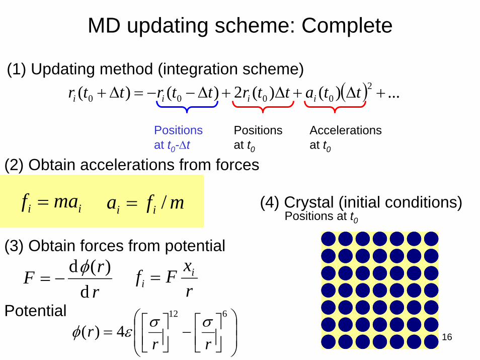
MD updating scheme: Complete

( ) ...)()(2)()( 20000 +Δ+Δ+Δ−−=Δ+ ttattrttrttr iiii

ii maf =

Positions at t0

Accelerationsat t0

Positions at t0-Δt

mfa ii /=

rxFf i

i =

(1) Updating method (integration scheme)

(2) Obtain accelerations from forces

(3) Obtain forces from potential

Potential

⎟⎟⎠

⎞⎜⎜⎝

⎛⎥⎦⎤

⎢⎣⎡−⎥⎦

⎤⎢⎣⎡=

612

4)(rr

r σσεφ

(4) Crystal (initial conditions)Positions at t0

rrF

d)(dφ

−=

17

2.2 How to model metals: Multi-body potentials

Pair potential: Total energy sum of all pairs of bondsIndividual bond contribution does not depend on other atoms“all bonds are the same”

∑ ∑≠= =

=N

jii

N

jijtotal rU

,1 121 )(φ

Is this a good assumption?

Courtesy of the Center for Polymer Studies at Boston University. Used with permission.

18

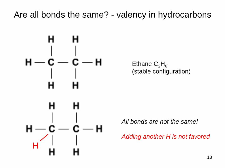
Are all bonds the same? - valency in hydrocarbons

H

All bonds are not the same!

Adding another H is not favored

Ethane C2H6(stable configuration)

19

Are all bonds the same? – metallic systems

Bonds depend on the environment!

Pair potentials: All bonds are equal!Reality: Have environmenteffects; it matter that there is a free surface!

+ differentbond EQ distance

stronger

Surface

Bulk

20

Are all bonds the same?

Bonding energy of red atom in is six times bonding energy in

This is in contradiction with both experiments and more accurate quantummechanical calculations on many materials

∑=

=N

jiji rU

1

)( φBonding energy of atom i

∑=

=6

1

)(j

iji rU φ )( iji rU φ=

After: G. Ceder

21

Are all bonds the same?

Bonding energy of red atom in is six times bonding energy in

This is in contradiction with both experiments and more accurate quantummechanical calculations on many materials

For pair potentials

For metals

Bonds get “weaker” as more atoms are added to central atom

Z~

Z~

:Z Coordination = how many immediate neighbors an atom has

After: G. Ceder

22

Bond strength depends on coordination

2 4 6 8 10 12 coordination

energy per bond

Z~

Z

Z~

pair potential

Nickel

Daw, Foiles, Baskes, Mat. Science Reports, 1993

23

Transferability of pair potentials

Pair potentials have limited transferability:

Parameters determined for molecules can not be used for crystals, parameters for specific types of crystals can not be used to describe range of crystal structures

E.g. difference between FCC and BCC can not be captured using a pair potential

24

Metallic bonding: multi-body effects

Need to consider more details of chemical bonding to understand environmental effects

+ + + + + ++ + + + + +

+ + + + + +

+Electron (q=-1)

Ion core (q=+N)

Delocalized valence electrons moving between nuclei generate a binding force to hold the atoms together: Electron gas model (positive ions in a sea of electrons)

Mostly non-directional bonding, but the bond strength indeed depends on the environment of an atom, precisely the electron density imposed by other atoms

25

Concept: include electron density effects

ρπ

Each atom features a particular distribution of electron density

j,ρπ

26


Electron density at atom i

Atomic electron density contribution of atom j to atom i

ij

)(, ijj rρπ

ijr

Contribution to electron density at site i due to electron density of atom j evaluated at distance rij

ijijijNj

ji xxrrneigh

−== ∑=

)(..1

,ρπρ

27


)()(21

..1i

Njiji Fr

neigh

ρφφ += ∑=

Electron density at atom i

embedding term F (how local electron density contributes to potential energy)

ixi

jxj

ijijijNj

ji xxrrneigh

−== ∑=

)(..1

,ρπρ)(, ijj rρπ

Atomic electron density contribution of atom j to atom i

28

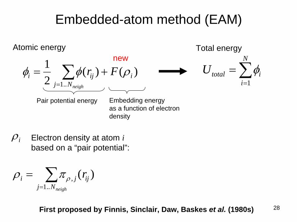
Embedded-atom method (EAM)

)()(21

..1i

Njiji Fr

neigh

ρφφ += ∑=

Pair potential energy Embedding energyas a function of electron density

iρ Electron density at atom ibased on a “pair potential”:

∑=

=neighNj

ijji r..1

, )(ρπρ

newAtomic energy

∑=

=N

iitotalU

1

φ

Total energy

First proposed by Finnis, Sinclair, Daw, Baskes et al. (1980s)

29

Embedding term: example

∑=

⎟⎠⎞

⎜⎝⎛ +=

neighNjiiji Fr

..1

)()(21 ρφφ

Embedding energyas a function of electron density

Pair potential energy

Embedding energy

Electron densityImage by MIT OpenCourseWare.

0 0.01 0.02 0.03 0.04 0.05 0.06-10

-5

0

G (e

V)

� (A-3)ρ o

30

Pair potential term: example

Pair contribution

Pair potential energy

Embedding energyas a function of electron density

)( ijrφ

ijrDistance∑=

⎟⎠⎞

⎜⎝⎛ +=

neighNjiiji Fr

..1

)()(21 ρφφ


2

1.5

1

0.5

02 3 4

R (A)o

U (e

V)

31

Effective pair interactions

Can describe differences between bulk and surface

r

+ + + + + ++ + + + + ++ + + + + +

r

+ + + + + ++ + + + + ++ + + + + +

See also: Daw, Foiles, Baskes, Mat. Science Reports, 1993


Bulk

Surface

Effe

ctiv

e pa

ir po

tent

ial (

eV )

1

0.5

0

-0.53 42

r (A)o

32

Comparison with experiment

33

Diffusion: Activation energies

(in eV)Courtesy of Elsevier, Inc., http://www.sciencedirect.com. Used with permission.

http://www.sciencedirect.com/

34

Comparison EAM model vs. experiment

Melting temperature (in K)

35

Summary: EAM method

State of the art approach to model metalsVery good potentials available for Ni, Cu, Al since late 1990s, 2000sNumerically efficient, can treat billions of particlesNot much more expensive than pair potential (approximately three times), but describes physics much better

Strongly recommended for use!

36

3. Brittle versus ductile materials

37

Tensile test of a wire

Image by MIT OpenCourseWare. Image by MIT OpenCourseWare.

Brittle Ductile

Strain

Stre

ss

BrittleDuctile

Necking

38

Ductile versus brittle materials

Difficultto deform,breaks easily

BRITTLE DUCTILE

Glass Polymers Ice...

Shear load

Copper, Gold

Easy to deformhard to break


43

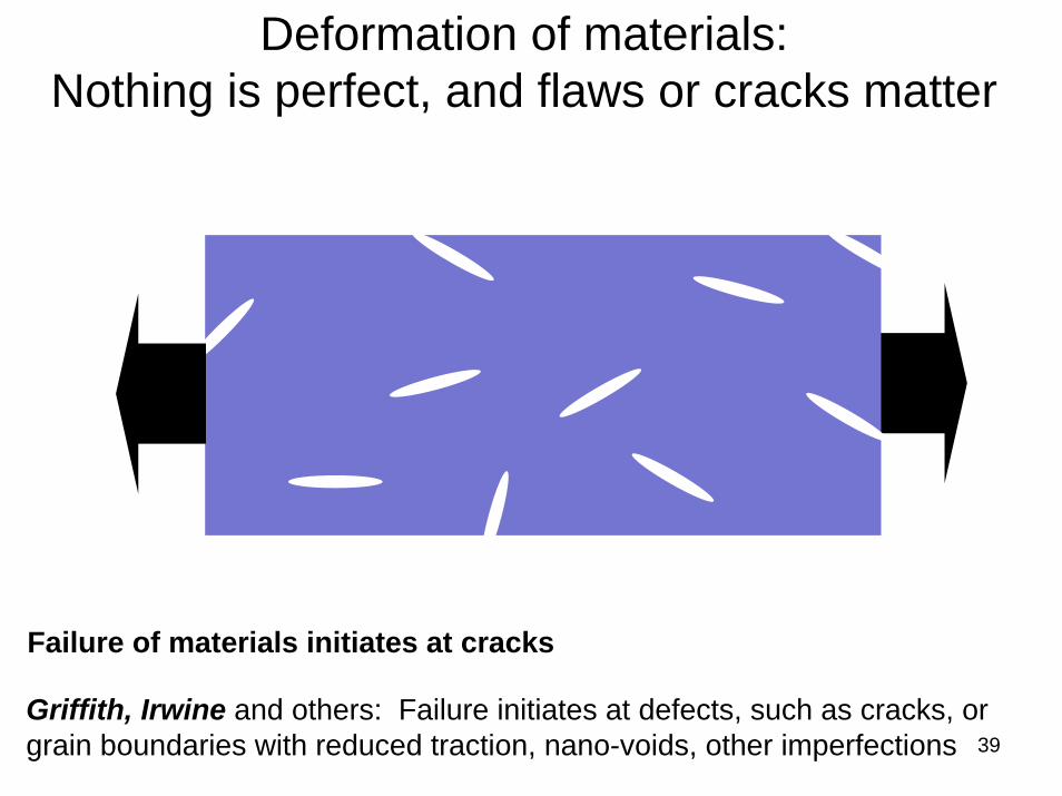
39Griffith, Irwine and others: Failure initiates at defects, such as cracks, or grain boundaries with reduced traction, nano-voids, other imperfections

Deformation of materials:Nothing is perfect, and flaws or cracks matter

Failure of materials initiates at cracks

40

SEM picture of material: nothing is perfect

41

Significance of material flaws

Stress concentrators: local stress >> global stress

“local”

“global”

Fig. 1.3 in Buehler, Markus J. Atomistic Modeling of Materials Failure. Springer, 2008. © Springer. All rights reserved. This content is excluded from our Creative Commons license. For more information, see http://ocw.mit.edu/fairuse.


42

“Macro, global”

“Micro (nano), local”

)(rσ r

Deformation of materials:Nothing is perfect, and flaws or cracks matter

Griffith, Irwine and others: Failure initiates at defects, such as cracks, or grain boundaries with reduced traction, nano-voids, other imperfections

Failure of materials initiates at cracks

43

Cracks feature a singular stress field, with singularity at the tip of the crack

rr 1~)(σ

:IK

stress tensor

Stress intensity factor (function of geometry)


σxy

σrθσrr

σθθ

σxx

σyy

r

x

y

θ

44

Crack extension: brittle response

Large stresses lead to rupture of chemicalbonds between atoms

Thus, crack extends

)(rσ

r


45

Lattice shearing: ductile response

Instead of crack extension, induce shearing of atomic latticeDue to large shear stresses at crack tipLecture 5



τ

τ

τ

τ

46

Brittle vs. ductile material behavior

Whether a material is ductile or brittle depends on the material’s propensity to undergo shear at the crack tip, or to break atomic bonds that leads to crack extension

Intimately linked to the atomic structure and atomic bonding

Related to temperature (activated process); some mechanism are easier accessible under higher/lower temperature

Many materials show a propensity towards brittleness at low temperature

Molecular dynamics is a quite suitable tool to study these mechanisms, that is, to find out what makes materials brittle orductile

Historical example: significance of brittle vs. ductile fracture

Liberty ships: cargo ships built in the U.S. during World War II (during 1930s and 40s)Eighteen U.S. shipyards built 2,751 Liberties between 1941 and 1945Early Liberty ships suffered hull and deck cracks, and several were lost to such structural defects

Twelve ships, including three of the 2710 Liberties built, broke in half without warning, including the SS John P. Gaines (sank 24 November 1943)

Constance Tipper of Cambridge University demonstrated that the fractures were initiated by the grade of steel used which suffered from embrittlement. She discovered that the ships in the North Atlantic were exposed to temperatures that could fall below a critical point when the mechanism of failure changed from ductile to brittle, and thus the hull could fracture relatively easily.

47

48

Liberty ships: brittle failure

Courtesy of the U.S. Navy.

49

4. Basic deformation mechanism in brittle materials - crack extension

50

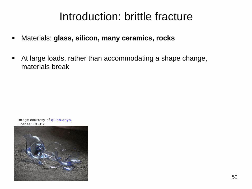
Introduction: brittle fracture

Materials: glass, silicon, many ceramics, rocks

At large loads, rather than accommodating a shape change, materials break

Image courtesy of quinn.anya. License: CC-BY.

http://www.flickr.com/photos/quinnanya/

51

Science of fracture: model geometry

Typically consider a single crack in a crystalRemotely applied mechanical loadFollowing discussion focused on single cracks and their behavior


remote load

remote load

a

52

Brittle fracture loading conditionsCommonly consider a single crack in a material geometry, under three types of loading: mode I, mode II and mode III

Tensile load, focus of this lecture


Mode I Mode II Mode III

Tensile load, focus of this lecture

53

Brittle fracture mechanisms: fracture is a multi-scale phenomenon, from nano to macro

Image removed due to copyright restrictions. See Fig. 6.2 in Buehler, Markus J. Atomistic Modeling of Materials Failure. Springer, 2008.

54

Focus of this part

Basic fracture process: dissipation of elastic energy

Fracture initiation, that is, at what applied load to fractures initiate

Fracture dynamics, that is, how fast can fracture propagate in material

55

Basic fracture process: dissipation of elastic energy

δa

Undeformed Stretching=store elastic energy Release elastic energydissipated into breaking chemical bonds

56

Elasticity = reversible deformation

Across-sectionalarea

Stress?

Force per unit area

57


AF /=σA

cross-sectionalarea

Stress?

Force per unit area

58


area under curve: stored energy

AF /=σ

Lu /Δ=ε

Across-sectionalarea

εσ E=

Young’s modulus

59

Continuum description of fractureFracture is a dissipative process in which elastic energy is dissipated to break bonds (and to heat at large crack speeds)Energy to break bonds = surface energy γs (energy necessary to create new surface, dimensions: energy/area, Nm/m2)

(1)(2)

a

δa

~

a~

"Relaxed"element

"Strained"element

ξ

a

σ

σ


60


E

2

21 σ

σ

ε

BaE

VE

WP~

21

21)1(

22

ξσσ== B out-of-plane thickness

0)2( =PW


(1)(2)

a

δa

~

a~

"Relaxed"element

"Strained"element

ξ

a

σ

σ

61


change of elastic (potential) energy

E

2

21 σ

σ

ε

BaE

VE

WP~

21

21)1(

22

ξσσ==

0)2( =PWBa

EWW PP

~21)1()2(

2

ξσ=−

(1)(2)

a

δa

~

a~

"Relaxed"element

"Strained"element

ξ

a

σ

σ


62


!

energy to create surfaces


E

2

21 σ

σ

ε

BaE

VE

WP~

21

21)1(

22

ξσσ==

0)2( =PWBaBa

EWW sPP

~2~21)1()2(

2

γξσ==−

(1)(2)

a

δa

~

a~

"Relaxed"element

"Strained"element

ξ

a

σ

σ Image by MIT OpenCourseWare.

63

!




E

2

21 σ

σ

ε

BaE

VE

WP~

21

21)1(

22

ξσσ==

0)2( =PWBaBa

EWW sPP

~2~21)1()2(

2

γξσ==−

ξγσ Es4

=

(1)(2)

a

δa

~

a~

"Relaxed"element

"Strained"element

ξ

a

σ

σ Image by MIT OpenCourseWare.

64


aBs~2γ=

!Ba

E~

21 2

ξσ=


ξγσ Es4

=

E

2

21 σ

σ

ε

change of elastic (potential) energy = G

(1)(2)

a

δa

~

a~

"Relaxed"element

"Strained"element

ξ

a

σ

σ


65

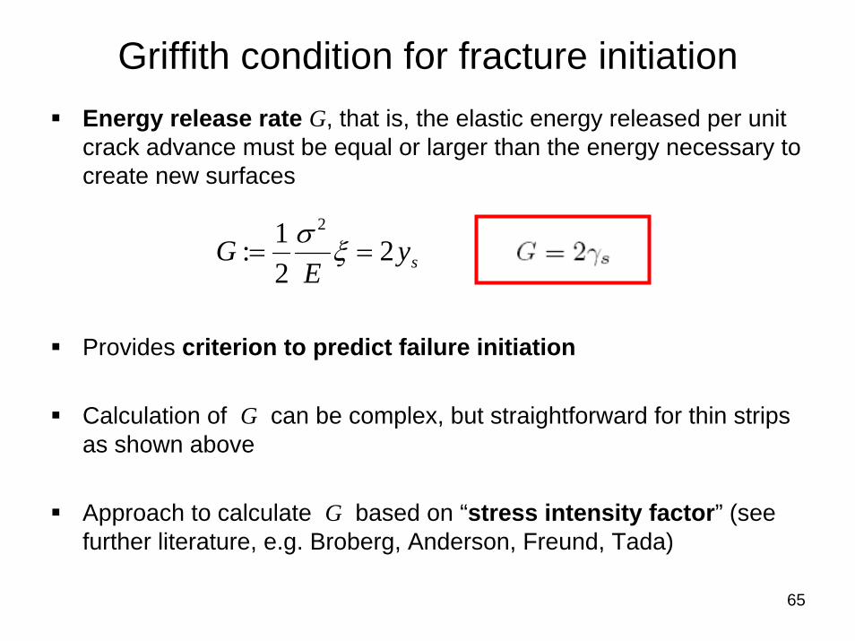
Griffith condition for fracture initiationEnergy release rate G, that is, the elastic energy released per unit crack advance must be equal or larger than the energy necessary to create new surfaces

Provides criterion to predict failure initiation

Calculation of G can be complex, but straightforward for thin strips as shown above

Approach to calculate G based on “stress intensity factor” (see further literature, e.g. Broberg, Anderson, Freund, Tada)

syE

G 221:

2

== ξσ

66

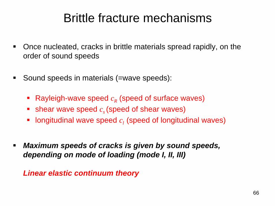
Brittle fracture mechanisms

Once nucleated, cracks in brittle materials spread rapidly, on the order of sound speeds

Sound speeds in materials (=wave speeds):

Rayleigh-wave speed cR (speed of surface waves)shear wave speed cs (speed of shear waves)longitudinal wave speed cl (speed of longitudinal waves)

Maximum speeds of cracks is given by sound speeds, depending on mode of loading (mode I, II, III)

Linear elastic continuum theory

67

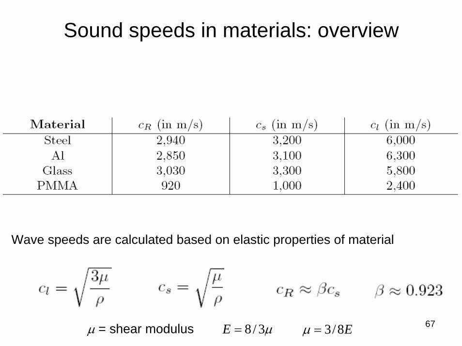
Sound speeds in materials: overview

Wave speeds are calculated based on elastic properties of material

μ = shear modulus μ3/8=E E8/3=μ

Limiting speeds of cracks: linear elastic continuum theory

• Cracks can not exceed the limiting speed given by the corresponding wave speeds unless material behavior is nonlinear• Cracks that exceed limiting speed would produce energy (physically impossible - linear elastic continuum theory)


68

Linear Nonlinear

Mode I

Mode II

Mode III

Limiting speed v

Limiting speed v

Cr Cs

Cs

Cl

Cl

Subsonic Supersonic

SupersonicIntersonicSub-RayleighSuper-

Rayleigh

Mother-daughter mechanism

69

Physical reason for crack limiting speedPhysical (mathematical) reason for the limiting speed is that it becomes increasingly difficult to increase the speed of the crack by adding a larger loadWhen the crack approaches the limiting speed, the resistance to fracture diverges to infinity (=dynamic fracture toughness)

Image removed due to copyright restrictions.Please see: Fig. 6.15 in Buehler, Markus J. Atomistic Modeling of Materials Failure. Springer, 2008.

70

Linear versus nonlinear elasticity=hyperelasticity

Linear elasticity: Young’s modulus (stiffness) does not changewith deformationNonlinear elasticity = hyperelasticity: Young’s modulus (stiffness) changes with deformation


Str

ess

Strain

Stiffen

ing

Softening

HyperelasticityLine

ar the

ory

71

Subsonic and supersonic fracture

Under certain conditions, material nonlinearities (that is, the behavior of materials under large deformation = hyperelasticity)becomes important

This can lead to different limiting speeds than described by the model introduced above

large deformationnonlinear zone

“singularity”

Deformation field near a crack

small deformation

rr 1~)(σ


Strain

Str

ess

Line

ar e

last

ic

clas

sica

l the

ories

Nonlinear real

materials

72

Limiting speeds of cracks

• Under presence of hyperelastic effects, cracks can exceed the conventional barrier given by the wave speeds• This is a “local” effect due to enhancement of energy flux• Subsonic fracture due to local softening, that is, reduction of energy flux


73

Stiffening vs. softening behavior

Increased/decreased wave speed

E

2

21 σ

σ

ε

“linear elasticity”

real materials


Str

ess

Strain

Stiffen

ing

Softening

HyperelasticityLine

ar the

ory

74

Energy flux reduction/enhancement

Energy flux related to wave speed: high local wave speed, high energy flux,crack can move faster (and reverse for low local wave speed)


Classical

New

Fracture process zoneHyperelastic zone

K dominance zone Characteristic energy length

Energy Flux Related to Wave Speed: High local wave speed, high energy flux, crack can move faster (and reversefor low local wave speed).

75

Physical basis for subsonic/supersonic fracture

Changes in energy flow at the crack tip due to changes in local wave speed (energy flux higher in materials with higher wave speed)Controlled by a characteristic length scale χ

Reprinted by permission from Macmillan Publishers Ltd: Nature. Source: Buehler, M., F. Abraham, and H. Gao. "Hyperelasticity Governs Dynamic Fracture at a Critical Length Scale." Nature 426 (2003): 141-6. © 2003.

76

Summary: atomistic mechanisms of brittle fracture

Brittle fracture – rapid spreading of a small initial crack

Cracks initiate based on Griffith condition G = 2γs

Cracks spread on the order of sound speeds (km/sec for many brittle materials)

Cracks have a maximum speed, which is given by characteristic sound speeds for different loading conditions)

Maximum speed can be altered if material is strongly nonlinear, leading to supersonic or subsonic fracture

77

Supersonic fracture: mode II (shear)

Please see: Buehler, Markus J., Farid F. Abraham, and Huajian Gao. "Hyperelasticity Governs Dynamic Fracture at a Critical Length Scale."Nature 426 (November 13, 2003): 141-146.

Appendix: Notes for pset #1

78

Notes regarding pset #1 (question 1.)

79

⎟⎟⎠

⎞⎜⎜⎝

⎛−=

TkEDDB

bexp0

TkEDDB

b−= )ln()ln( 0

)ln(D

)ln( 0D

T1

B

b

kE

−~

slope

Plot data extracted from RMSD graph, then fit equation above and identify parameters

high temperature low temperature

Mechanism and energy barrier

80

bE

Courtesy of Runningamok19. License: CC-BY.

attempt of Rate :0D

“transition state”

⎟⎟⎠

⎞⎜⎜⎝

⎛−=

TkEDDB

bexp0

http://en.wikipedia.org/wiki/File:Chemical_surface_diffusion_slow.gif

MIT OpenCourseWarehttp://ocw.mit.edu

3.021J / 1.021J / 10.333J / 18.361J / 22.00J Introduction to Modeling and SimulationSpring 2012

For information about citing these materials or our Terms of use, visit http://ocw.mit.edu/terms.

http://ocw.mit.edu/

http://ocw.mit.edu/terms

Documents

How to model chemical interactions II · 1. Atoms, molecules, chemistry 2. Continuum modeling approaches and solution approaches 3. Statistical mechanics 4. Molecular dynamics, Monte