INDUSTRY REPORT

How Much Rainfall Becomes Runoff?

Loss modelling for flood estimation

How Much RainfallBecomes Runoff?

Loss modelling for floodestimation

by

Peter Hill, Russell Mein and Lionel Siriwardena

Industry ReportReport 98/5

June 1998

ii

Hill, P. I. (Peter Ian)

How much rainfall becomes runoff?: loss modelling for flood estimation.

Bibliography

ISBN 1 876006 26 9.

1. Runoff – Australia.

2. Runoff – Australia – Mathematical models

3. Flood forecasting – Australia

4. Flood forecasting – Australia – Mathematical models. I Siriwardena, L.

(Lionel), 1953–. II. Mein, Russell G. III. Cooperative Research Centre for

Catchment Hydrology. IV. Title. (Series: Report (Cooperative Research

Centre for Catchment Hydrology): 98/5).

551.4880994

ISSN 1039-7361

Keywords

Floods and Flooding

Rainfall/Runoff Relationship

Modelling (Hydrological)

Frequency Analysis

Design Data

Infiltration

Water Flow

Catchment Areas

Flood Forecasting

© Cooperative Research Centre for Catchment Hydrology, 1998

Cooperative Research Centre for Catchment Hydrology

Centre Office

Department of Civil Engineering

Monash University

Clayton, Victoria, 3168

Australia

Telephone: (03) 9905 2704

Fax: (03) 9905 5033

Home page: http://www-civil.eng.monash.edu.au/centres/crcch/

Photographs were provided by:

• Ian Rutherfurd (front and back cover)

• Mat Gilfedder

• Bureau of Meteorology – Mike Rosel

Background cover photo: Aerial view of Murray River billabong near Albury, NSW.

iii

This Industry Report is one of a series prepared by the Cooperative Research Centre (CRC) for Catchment Hydrology to help provide

the Australian land- and water-use industry with improved ways of managing catchments.

Through this series of reports and other forms of technology transfer, industry is now able to benefit from the Centre’s high-

quality, comprehensive research on salinity, forest hydrology, waterway management, urban hydrology and flood hydrology.

This particular Report represents a major contribution from the CRC’s flood hydrology program, and presents key findings

from the project entitled ‘Improved Loss Modelling for Design Flood Estimation and Flood Forecasting’. (More detailed

explanations and research findings from the project can be found in a separate series of Research Reports and Working

Documents published by the Centre.)

The CRC welcomes feedback on the work reported here, and is keen to discuss opportunities for further collaboration with

industry to expedite the process of getting research outcomes into practice.

Russell Mein

Director, CRC for Catchment Hydrology

Foreword

iv

This report summarises the Cooperative Research Centre (CRC) for Catchment Hydrology’s research on Project D1: ‘Improved Loss Modelling for Design Flood

Estimation and Flood Forecasting’.

The need for research to quantify losses from rainfall was identified by a technical advisory group (TAG) comprising researchers and practitioners involved

in flood estimation. The group suggested a number of lines of research to pursue, and these were followed up. The empirical analysis of the large database of

rainfall and runoff events collated for the study was a key to the successful project outcomes.

This report concentrates on the derivation of new loss parameters, and on the development of a new loss model for real-time flood forecasting.

These outcomes are seen to be of immediate use to practitioners. Other sub-projects, not discussed here, were:

• extension of data sets using continuous models (Elma Kazazic)

• measurement of the spatial distribution of soil moisture in forested catchments (Leon Soste)

• application of point infiltration equations at catchment scale (Jason Williams)

• development of a design flood estimation procedure using data generation and a daily water balance model (Walter Boughton and Peter Hill).

People involved in this project were Peter Hill (Project Leader) and Lionel Siriwardena, assisted by Nanda Nandakumar (in the early stages), Upula Maheepala,

Leon Soste, Elma Kazazic and Russell Mein (Program Leader). The project reference panel (Jim Elliott, Tom McMahon, Russell Mein, Rory Nathan and Erwin

Weinmann) gave important guidance on the work. Walter Boughton was a significant contributor.

Preface

Foreword iii

Preface iv

Introduction 1

• What is rainfall loss? 1

• Losses at catchment scale

Applying a point infiltration equation 2

PART A: Losses for design flood estimation 3

• Rainfall-based design flood estimation 3

• Losses recommended in Australian Rainfall & Runoff (1987) 3

Developing new design losses 4

• Results 6

• Burst initial loss 7

• Seasonal variation of losses 7

• How does loss vary with rainfall severity? 7

• Prediction equations 8

Difficulties 8

Results 9

Seasonal adjustment 9

Predicting baseflow index for ungauged catchments 10

Testing new design inputs 10

• Selected catchments 10

• Flood frequency analysis 11

• RORB modelling 11

• Results using AR&R design values 12

• Effect of new areal reduction factors 12

• New design losses 13

• Summary of design loss work 14

PART B: Losses for flood forecasting 15

• Real-time flood forecasting 15

• Soil moisture 15

• Pilot study results 15

A variable proportional loss model 16

• Applying the model 17

• Regionalisation of model parameters 17

• Advantages 18

• Limitations 19

• Summary of flood forecasting work 19

Conclusions 20

• Part A: Losses for design flood estimation 20

• Part B: Losses for flood forecasting 20

Further reading 21

Appendix A: Values of Baseflow Index

Contents

v

1

IN T R O D U C T I O N

The answer to the question “How much rainfall becomes runoff?” is of

fundamental hydrologic importance. In flood hydrology, the proportion

of runoff from a storm has a major influence on the size of the resulting

flood. The amount of rain which does not become runoff is termed “loss”.

The objectives of CRC Project D1 ‘Improved Loss Modelling for Design

Flood Estimation and Flood Forecasting’ were to:

• develop loss models which reduce the uncertainty in design flood

hydrographs (used for sizing of hydraulic structures); and

• develop loss models for real-time flood forecasting (to make forecasts

of flood levels more accurate).

This section briefly covers the concept of rainfall losses, and the

importance of predicting them at catchment scale.

Then follow two main sections, corresponding to the two objectives above:

Part A describes losses for design flood estimation. Limitations of the

currently recommended design losses are outlined, and the development of

new losses consistent with the design information in Australian Rainfall

and Runoff (AR&R, 1987) described.

An independent test was then undertaken to check:

• the application of existing design parameters, and

• the new design losses and areal reduction factors developed by the

CRC for Catchment Hydrology.

Part B describes the estimation of losses for real-time flood forecasting.

Two different measures of soil moisture are examined:

• the antecedent precipitation index, and

• pre-storm baseflow

to find the best predictor of loss.

A new variable proportional loss model, suitable for real-time flood

forecasting, is described.

The conclusions summarise the main findings of both sections.

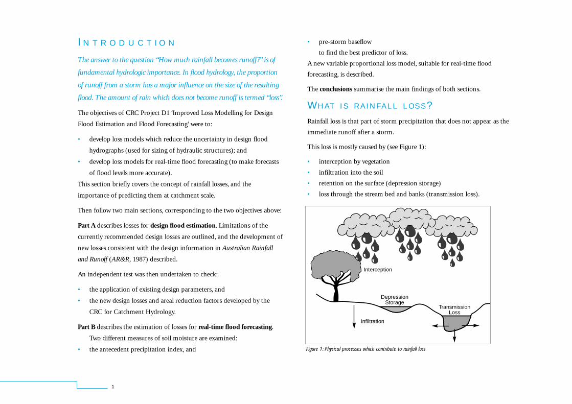
WH AT I S R A I N FA L L L O S S?Rainfall loss is that part of storm precipitation that does not appear as the

immediate runoff after a storm.

This loss is mostly caused by (see Figure 1):

• interception by vegetation

• infiltration into the soil

• retention on the surface (depression storage)

• loss through the stream bed and banks (transmission loss).

Figure 1: Physical processes which contribute to rainfall loss

DepressionStorage

Infiltration

TransmissionLoss

Interception

2

LO S S E S AT C AT C H M E N T S C A L E

The processes that contribute to rainfall loss may be well defined at

a point; the difficulty occurs in trying to estimate a representative value of

loss over an entire catchment. Spatial variability in topography, catchment

characteristics (such as vegetation and soils) and rainfall makes it difficult

to link the loss to catchment characteristics.

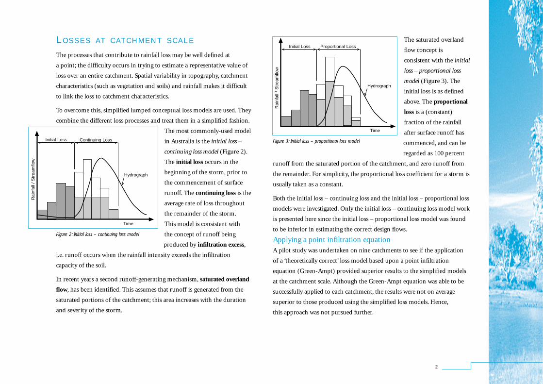
To overcome this, simplified lumped conceptual loss models are used. They

combine the different loss processes and treat them in a simplified fashion.

The most commonly-used model

in Australia is the initial loss –

continuing loss model (Figure 2).

The initial loss occurs in the

beginning of the storm, prior to

the commencement of surface

runoff. The continuing loss is the

average rate of loss throughout

the remainder of the storm.

This model is consistent with

the concept of runoff being

produced by infiltration excess,

i.e. runoff occurs when the rainfall intensity exceeds the infiltration

capacity of the soil.

In recent years a second runoff-generating mechanism, saturated overland

flow, has been identified. This assumes that runoff is generated from the

saturated portions of the catchment; this area increases with the duration

and severity of the storm.

The saturated overland

flow concept is

consistent with the initial

loss – proportional loss

model (Figure 3). The

initial loss is as defined

above. The proportional

loss is a (constant)

fraction of the rainfall

after surface runoff has

commenced, and can be

regarded as 100 percent

runoff from the saturated portion of the catchment, and zero runoff from

the remainder. For simplicity, the proportional loss coefficient for a storm is

usually taken as a constant.

Both the initial loss – continuing loss and the initial loss – proportional loss

models were investigated. Only the initial loss – continuing loss model work

is presented here since the initial loss – proportional loss model was found

to be inferior in estimating the correct design flows.

Applying a point infiltration equation

A pilot study was undertaken on nine catchments to see if the application

of a ‘theoretically correct’ loss model based upon a point infiltration

equation (Green-Ampt) provided superior results to the simplified models

at the catchment scale. Although the Green-Ampt equation was able to be

successfully applied to each catchment, the results were not on average

superior to those produced using the simplified loss models. Hence,

this approach was not pursued further.

Figure 3: Initial loss – proportional loss model

Figure 2: Initial loss – continuing loss model

Initial Loss Continuing Loss

Hydrograph

Time

Rai

nfal

l / S

trea

mflo

w

Initial Loss Proportional Loss

Hydrograph

Time

Rai

nfal

l / S

trea

mflo

w

3

Each component has a distribution of possible values, and the probability

of the calculated flood peak should theoretically account for the effect of

the combined probabilities. Because there is currently a lack of information

on the true distribution of each of the components and the complexity

involved, AR&R recommends taking some ‘central’ or ‘typical’ value for

each of the key inputs.

LO S S E S R E C O M M E N D E D I N AU S T R A L I A N

RA I N FA L L & RU N O F F (1987)The losses recommended in AR&R are ‘typical’ values obtained from

analysing the largest flood events observed in a catchment being studied.

PART A: LO S S E S F O R

D E S I G N F L O O D E S T I M A T I O N

Hundreds of millions of dollars are spent annually in Australia on

works whose size or location depends on an estimate of a design flood.

For all rainfall-based estimation methods, the design loss is a key factor

in the estimation of a design flood of a given chance of occurrence.

RA I N FA L L -B A S E D D E S I G N F L O O D

E S T I M AT I O N

Guidelines for rainfall-based design flood estimation are contained in

Australian Rainfall and Runoff (AR&R, 1987). This document recommends

an event-based methodology, and provides estimates of the different

parameters to be used in design.

The estimation of a

design flood hydrograph

with a specified annual

exceedance probability

(AEP) for a catchment,

begins with a design

rainfall of the same

AEP. As indicated in

Figure 4, the probability of the calculated design flood peak will depend

upon the choice of the critical storm duration, areal reduction factor,

rainfall temporal pattern, design losses, runoff model, model parameters

and the baseflow. Table 1: AR&R recommended design losses

Initial loss zeroContinuing loss 1.0–3.6 mm/h(depending on average recurrence intervals)

Initial loss 10–35 mm, varyingwith catchment size and meanannual rainfall.Continuing loss 2.5 mm/h

Initial loss 15 mmContinuing loss 4 mm/h

Continuing loss 2.5 mm/hInitial loss 25–35 mm (Melbourne Water)Initial loss 15–20 mm (Rural Water Commission)

Probably as for similar areas of NSW

ACT

New South WalesEast of the western slopes

Arid Zone, meanannual rainfall < 300 mm

VictoriaSouth and eastof the GreatDividing Range

North and westof the GreatDividing Range

Location Median values of parameters

Figure 4: Event-based design flood estimation

DesignRainfallDepth• Duration

• Areal reduction factor• Temporal pattern• Losses• Design model• Model parameters• Baseflow

DesignFloodPeak

4

DE V E L O P I N G N E W D E S I G N

L O S S E S

A study was undertaken to derive new design losses. Catchments were

selected using the following criteria:

• availability of good quality concurrent rainfall and streamflow data;

• small to medium sized rural catchments (catchment areas less than

approximately 150 km2);

• unregulated streamflow (no effects from storages upstream).

Losses were calculated for the 22 catchments from Victoria and the ACT

shown in Table 2. The location of the catchments is shown in Figure 6.

(Note: The identification code is used to label figures in this report)

Figure 6: Locations of selected catchments

Kilometers

0 50 100

NSW

N

VICTORIA

ACT

GL

AICH

FO

WA

GO

CALE

MY WN BO

MO

SPSN

LA

TATE

CO

TI

OR

JE

GI

A summary of the recommended design losses for south-eastern Australia

contained in AR&R is shown in Table 1. No recommendation is made for

initial loss for Tasmania. There is a large range of values, with no guidance

as to how the losses may vary with catchment characteristics. In addition

there is no separate information available for the areas of Victoria north

and west of the Great Dividing Range.

The recommended continuing loss

values in Table 1 are average values.

In practice, continuing loss for a

catchment is highly variable, as

shown in Figure 5.

In addition to the scarcity of

information on design losses, most

loss values were derived from

analysing large runoff events.

AR&R identifies two inadequacies

in the loss values:

• The selection of large runoff events for loss derivation is biased towards

wet antecedent conditions, as not all high rainfall events result in high

runoff events. i.e. Losses tend to be too low.

• Loss values related to complete storm events (storm losses) do not

account for the nature of the design rainfall information in Chapters 2

and 3 of AR&R, which has been derived from intense bursts of rainfall

within longer duration storms. i.e. Losses tend to be too high.

AR&R recognises that these two inadequacies should have opposite effects;

it is implicitly assumed by users of the current design loss values that they

compensate one for the other.

105

Figure 5: Frequency distribution of individual lossrate (from AR&R)

5

For each selected rainfall event, the time of first surface runoff (if any) was

noted to calculate storm initial loss. The continuing loss was determined to

preserve the volume balance of rainfall and runoff.

It was then necessary to consider the estimation of losses for bursts of

rainfall embedded within longer duration storms. The difference between

the initial loss for a burst and for a storm is illustrated in Figure 7. The

initial loss for the storm is assumed to be the depth of rainfall before

surface runoff begins. The initial loss for the burst, however, is the part of

the storm initial loss which occurs within the burst. The burst initial loss

depends on the position of the burst within the storm. It can range from

zero (if the burst occurs after surface runoff has commenced) up to the full

storm initial loss.

The initial loss values contained in AR&R represent storm initial losses.

However, the burst initial loss should be used for design.

Losses were calculated to be consistent with the design rainfalls, i.e.

estimated from intense bursts of rainfalls embedded within longer duration

storms. This avoided the problem with losses calculated from events

selected on the basis of runoff. All bursts of rainfall that had an average

recurrence level (ARI) of more than a year were selected. Losses were

calculated for 1,059 bursts of rainfall over the 22 catchments.

Table 2: Selected catchments

Tidbinbilla Ck @ Mountain Creek TI 25 1120

Chapple Ck @ Chapple Vale CH 28 1520

Goodman Ck above Lerderderg Tunnel GO 32 800

Campaspe River @ Ashbourne CA 33 960

Tarwin River East Branch @ Mirboo TA 43 1140

Ginninderra Ck u/s Barton Highway GI 48 640

Snobs Ck @ Snobs Ck Hatchery SN 51 1660

Myers Ck @ Myers Flat MY 55 520

Jerrabomberra Ck @ Four Mile Creek JE 55 610

Ford River @ Glenaire FO 56 1520

Glenelg River @ Big Cord GL 57 680

Warrambine Ck @ Warrambine WA 57 660

Spring Ck @ Fawcett SP 60 720

La Trobe River @ Near Noojee LA 62 1480

Orroral River @ Crossing OR 90 750

Aire River @ Wyelangta AI 90 1880

Moonee Ck @ Lima MO 91 1060

Cobbannah Ck @ Bairnsdale CO 106 840

Boggy Ck @ Angleside BO 108 1080

Wanalta Ck @ Wanalta WN 108 540

Tarwin R East Branch @ Dumbalk Nth TE 127 1140

Lerderderg River @ Sardine Ck LE 153 1080

Catchment Code Area Rainfall(km2) (mm)

Figure 7: Initial loss for an embedded rainfall burst

Storm Burst

Burst Initial Loss (ILb)

Storm Initial Loss (ILs)

Flood Hydrograph

Time

Rai

nfal

l / S

trea

mflo

w

6

RE S U LT S

The mean storm losses and the typical range of variation between events

for each catchment are shown in Figures 8 and 9.

It is worth noting that several of the mean values of storm initial loss are

outside (generally higher than) the range of values given in AR&R (Table 1).

For continuing loss, most values are higher than the recommended 2.5 mm/h.

BU R S T I N I T I A L L O S S

In the previous section, the mean storm initial losses are summarised.

They do not however account for the embedded nature of the design

rainfalls contained in AR&R, ie they are bursts of rainfall within longer

duration storms. It is therefore expected that the initial loss suitable for

design (the burst initial loss; ILb) should be lower than that obtained for

the complete storm (the storm initial loss; ILs).

Examination of the mean ratios of ILb to ILs showed a weak trend with

mean annual rainfall (MAR); wetter catchments having generally lower

values of ILb/ILs . In order to derive a value of ILb for design, an equation

was fitted to the mean values of ILb/ILs from each duration and catchment.

While the relatively low values of r2 indicate considerable scatter about the

fitted line, even after allowing for the effect of mean annual rainfall, the

relationship should provide a satisfactory basis for probability-based design.

Nevertheless, it should be remembered that there is a significant chance of

ILb/ILs being close to zero, even for longer duration bursts.

Figure 9: Mean continuing loss by catchment (identification codes in Table 2)

Figure 8: Mean storm initial loss by catchment (identification codes in Table 2)

90% confidence limits about mean

90% confidence limits about mean

80

70

60

50

40

30

20

10

0

14.0

12.0

10.0

8.0

6.0

4.0

2.0

0.0

TI

CH

GO

CA TA GI

SN

MY JE FO GL

WA

SP LA OR AI

MO

CO

BO

WN TE LE

Mea

n St

orm

Initi

al L

oss

(mm

)

Catchment

Catchment

Mea

n Co

ntin

uing

Los

s (m

m)

TI

CH

GO

CA TA GI

SN

MY JE FO GL

WA

SP LA OR AI

MO

CO

BO

WN TE LE

(1)

7

HO W D O E S L O S S VA RY W I T H R A I N FA L L

S E V E R I T Y? The answer is difficult because of the lack of severe rainfall events in the

recorded data (see Figure 12). More than half of the bursts analysed had

average recurrence intervals (ARIs) of less than two years; only 4 percent

of bursts had ARIs of greater than 20 years.

There were not enough individual-catchment events to study the variation

of losses with ARI, so the data were again standardised by dividing by the

mean loss for the

catchment and then

pooled.

The derived loss

parameters for each of

the bursts are plotted

against ARI in Figures

13 and 14, and show

SE A S O N A L VA R I AT I O N O F L O S S E S

In the above sections, mean losses were derived for each catchment without

considering how these losses varied seasonally. Initial loss, and possibly

continuing losses, are related to antecedent moisture; hence a seasonal

variation in derived losses is likely.

The number of storms for individual catchments was not sufficient to study

the seasonal variation of derived losses for individual catchments, so the

data were standardised by dividing by the mean loss for each catchment and

then pooled. The mean standardised loss for all catchments was then

calculated for each month, and a sinusoidal curve fitted (Figures 10 and 11)

to the values.

These curves confirm that there is a distinct seasonal variation of losses

which is adequately represented by sinusoidal relationships.

Figure 12: Distribution of burst ARIs

2 4 6 8 10 12 14 16 18 20 >20

% o

f V

alu

e

Average Recurrence Interval (years)

2

60

50

40

30

20

10Figure 10: Monthly variation of storm initial loss (pooled data)

Month

Stan

dard

ised

ILs

0

0.2

0.4

0.6

0.8

1

1.2

1.4

1.6

1.8

0 1 2 3 4 5 6 7 8 9 10 11 12

monthly mean

fitted Sine curve

upper 90% limit

lower 90% limit

ILs = 1.0 + 0.381 Sin [0.1667 π (month + 0.413)]r2 = 0.80, SE = 0.14

Figure 11: Monthly variation of continuing loss (pooled data)

Month

Stan

dard

ised

CL

monthly mean

fitted Sine curve

upper 90% limit

lower 90% limit

CL = 1.0 + 0.303 Sin [0.1667 π (month + 1.55)]r2 = 0.75, SE = 0.13

8

that it is difficult to determine any loss trends with ARI. The data were also

grouped into three ranges according to their ARI, but no significant trend

was observed. The conclusion is that this study has produced no evidence

that the design loss rate varies with rainfall severity.

PR E D I C T I O N E Q U AT I O N S

The aim was to produce estimates of losses for any catchment in the region

represented by the data. For this, the results obtained from individual

catchments must be generalised – a process called regionalisation.

Difficulties

Many authors have concluded there is no relationship between mean losses

and characteristics of soil and vegetation at catchment scale. This failure to

relate losses to catchment characteristics may be due to the following:

• Variability that is not related to catchment characteristics may result

from difference in methods to estimate losses for different catchments.

• The loss from any storm depends strongly on antecedent conditions;

therefore the mean loss for a catchment will be affected by the sample

of events (storms) used. This is especially important given the strong

seasonal variation of losses noted earlier in this report.

• Calculated loss values reflect any errors in rainfall and streamflow data.

The variability of rainfall over an area, and the usually limited number

of raingauges, mean that estimates of catchment average rainfall (and

so the values of losses) are not reliable.

• Catchment characteristics vary spatially; soil hydraulic properties can

vary enormously over an area which seems to be similar terrain. This

makes it difficult to estimate representative parameters for a catchment.

• Little information is available on the hydraulic properties of soils.

The current classification of soils in Australia is based upon texture;

little work has been done on the classification of soils according to

hydraulic properties.

Figure 13: Variation of storm initial loss with ARI (all catchments)

ARI (years)

Stan

dard

ised

ILs

0

0.5

1

1.5

2

2.5

3

3.5

4

4.5

5

1 10 100 1000

Figure 14: Variation of continuing loss with ARI (all catchments)

ARI (years)

Stan

dard

ised

CL

0

0.5

1

1.5

2

2.5

3

3.5

4

4.5

1 10 100 1000

9

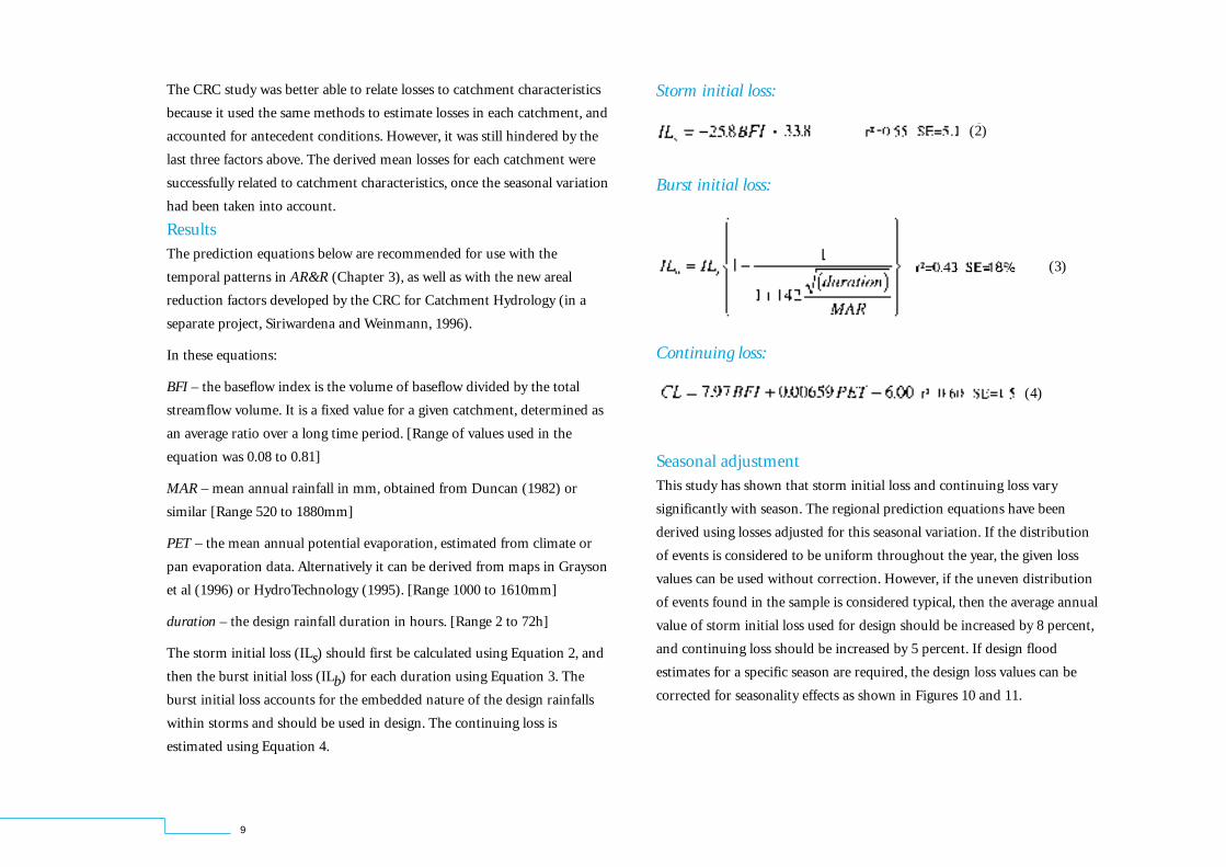
Storm initial loss:

Burst initial loss:

Continuing loss:

Seasonal adjustment

This study has shown that storm initial loss and continuing loss vary

significantly with season. The regional prediction equations have been

derived using losses adjusted for this seasonal variation. If the distribution

of events is considered to be uniform throughout the year, the given loss

values can be used without correction. However, if the uneven distribution

of events found in the sample is considered typical, then the average annual

value of storm initial loss used for design should be increased by 8 percent,

and continuing loss should be increased by 5 percent. If design flood

estimates for a specific season are required, the design loss values can be

corrected for seasonality effects as shown in Figures 10 and 11.

The CRC study was better able to relate losses to catchment characteristics

because it used the same methods to estimate losses in each catchment, and

accounted for antecedent conditions. However, it was still hindered by the

last three factors above. The derived mean losses for each catchment were

successfully related to catchment characteristics, once the seasonal variation

had been taken into account.

Results

The prediction equations below are recommended for use with the

temporal patterns in AR&R (Chapter 3), as well as with the new areal

reduction factors developed by the CRC for Catchment Hydrology (in a

separate project, Siriwardena and Weinmann, 1996).

In these equations:

BFI – the baseflow index is the volume of baseflow divided by the total

streamflow volume. It is a fixed value for a given catchment, determined as

an average ratio over a long time period. [Range of values used in the

equation was 0.08 to 0.81]

MAR – mean annual rainfall in mm, obtained from Duncan (1982) or

similar [Range 520 to 1880mm]

PET – the mean annual potential evaporation, estimated from climate or

pan evaporation data. Alternatively it can be derived from maps in Grayson

et al (1996) or HydroTechnology (1995). [Range 1000 to 1610mm]

duration – the design rainfall duration in hours. [Range 2 to 72h]

The storm initial loss (ILs) should first be calculated using Equation 2, and

then the burst initial loss (ILb) for each duration using Equation 3. The

burst initial loss accounts for the embedded nature of the design rainfalls

within storms and should be used in design. The continuing loss is

estimated using Equation 4.

(4)

(3)

(2)

10

Predicting baseflow index for ungauged catchments

The baseflow index (BFI), a useful indicator of catchment loss, is only

directly available for gauged catchments; however it appears to vary quite

smoothly between gauge locations. Appendix A shows a plot of derived BFI

values; from it a reasonable estimate of BFI can be made for locations in

much of Victoria.

Alternatively, Lacey (1996) has examined the prediction of BFI for

ungauged catchments. In his work, the native vegetation was identified and

classified for each catchment and combined with the underlying geology to

form geology – vegetation classes. Geology – vegetation classes explained

approximately 85 percent of the variation in BFI. This work allows

prediction of BFI for ungauged catchments based upon:

• the native vegetation, which is available from reports such as the Land

Conservation Council Victoria Reports or from an inspection of the

catchment

• the underlying geology, which is readily available from 1:250,000

geological maps.

TE S T I N G N E W D E S I G N I N P U T S

An independent test was undertaken to determine the effect on design

flood estimates of using

• existing AR&R parameters

• new areal reduction factors

• new design losses.

The testing was by comparison with results of flood frequency analysis, and

was undertaken for annual exceedance probabilities (AEPs) of 1 in 10 and 1

in 50.

SE L E C T E D C AT C H M E N T S

The testing was undertaken

on 10 catchments (nine in

Victoria and one from the

ACT) ranging in area from

32 to 332 square kilometres.

The catchments are listed in

Table 3 (eight were used to

derive the new losses, but

the test procedure is still

an independent assessment,

as shown below).

The catchments are shown

in Figure 15; they represent

a geographic spread

covering a large part of Victoria (with one in the ACT).

Table 3: Summary of selected catchments

Goodman Ck GO 32 1971 1995 25

Ford River FO 56 1970 1986 17

Orroral River OR 90 1968 1995 28

Aire River AI 90 1968 1995 28

Moonee Ck MO 91 1963 1995 33

Wanalta Ck WN 108 1961 1995 35

Tarwin River TE 127 1971 1995 25

Lerderderg River LE 153 1960 1995 36

Avon River AV 259 1965 1995 31

Seven Cks SE 332 1964 1995 32

Catchment Code Area Streamflow data(km2) start end years

11

RORB M O D E L L I N G

A RORB model was developed for each of the 10 catchments in Table 3.

The model subtracts losses from rainfall to produce rainfall-excess and

routes this through the catchment to produce a hydrograph at the point of

interest. The catchment is subdivided into a number of sub-areas to

account for catchment and channel storage, and allow spatially non-

uniform rainfall over the catchment. A consistent model definition and

calibration approach for the different catchments is important to reduce

result variability.

The RORB models were calibrated using the largest recorded flood events

which had streamflow and rainfall data. For each catchment, at least six

events were selected for calibration. Some of these events had data errors or

inconsistencies that affected the calibration; these events were discarded.

The final number of events used for calibration varied from four to eight

per catchment.

Apart from the two loss parameters in RORB, there are two routing

parameters that can be used for calibration:

m a measure of the catchment’s non-linearity: a value of 1 implies a linear

catchment

kc a measure of the storage in the catchment; the principal parameter of

the model.

In this study m was set to 0.8. The initial loss was varied so that the rising

limb of the calculated hydrograph matched the recorded hydrograph. The

kc was varied to match the peak flow.

FL O O D F R E Q U E N C Y A N A LY S I S

A flood frequency analysis of recorded peak flows was undertaken for each

catchment, with the log-Pearson III distribution being used for this purpose.

Flood estimates from the analysis were used to test the performance of the

‘old’ and ‘new’ rainfall-based, design peak flow estimates.

The occurrence of low flows in the annual series can have a significant

effect on fitting a frequency distribution to an annual series of flood peaks.

The annual series were checked for low flows. If present, these flows were

omitted and the probability adjustment recommended in AR&R applied.

Figure 15: Location of study catchments

Ford River

Aire River

Goodman Creek

Wanalta Creek

Seven CreeksMoonee Creek

Tarwin River

Orroral River

Lerderderg River

Avon River

Kilometers

0 50 100

12

RE S U LT S U S I N G AR&R D E S I G N VA L U E S

For this study, an initial loss of 20 mm and a continuing loss of

2.5 mm/h were adopted for all catchments to represent design losses

recommended in AR&R.

Information on design rainfall depths (IFD data), temporal patterns and

areal reduction factors was taken directly from AR&R. The losses were

applied to the design rainfalls, and the resultant rainfall excess routed

through the RORB models using the calibrated parameters. Design storms

from 1 to 72 hours were routed through the RORB model, and the critical

duration was estimated as that which gave the largest peak flow.

Following AR&R, the design surface runoff was then converted to

a design total flow by adding an estimate of the baseflow to the surface

runoff (the average of the baseflow for the calibration events).

The resulting peak flow was taken as the design peak flow for the given

annual exceedance probability, and compared to that obtained from the

flood frequency analysis.

Figure 16 shows the differences between the peak flows obtained using the

rainfall-based approach with AR&R design values, and using flood

frequency analysis. Clearly, from this figure, the use of the AR&R design

values results in over-estimation of the peak flows for seven of the 10

catchments. The average over-prediction is 47 percent for an AEP of 1 in 10

and 32 percent for an AEP of 1 in 50.

This independent test represents the application to ungauged catchments,

i.e. where design losses cannot be calibrated against the results from flood

frequency analysis.

EF F E C T O F N E W A R E A L R E D U C T I O N

FA C T O R S

Areal reduction factors

(ARFs) convert point

rainfall intensities to

average rainfall

intensities over a

catchment of a given

area. They take into

account the observation

that larger catchments

are less likely than small

catchments to have high

intensity rainfall over the whole catchment.

The ARFs in AR&R are based upon studies done in Chicago and Arizona in

the USA, because of a lack of Australian data. A major study was therefore

initiated, as part of CRC for Catchment Hydrology Project D3, to derive

new ARFs for Victoria (Siriwardena and Weinmann, 1996).

Figure 16: Comparison of flood estimates using frequency analysis of observed data and runoffrouting using AR&R parameters

-40

-20

0

20

40

60

80

100

120

140

Diff

eren

ce B

etw

een

Pea

k Fl

ows

(%)

GO FO OR AI MO WN TE LE AV SE

Catchment

AEP of 1 in 10AEP of 1 in 50

Figure 17: Effect of using new ARFs on the design flood peak

GO FO OR AI MO WN TE LE AV SE0

2

4

6

8

10

12

14

16

18

20

Red

uct

ion

in P

eak

Flo

w (

%)

GO FO OR AI MO WN TE LE AV SE

Catchment

AEP of 1 in 10AEP of 1 in 50

13

Design losses were estimated

for each catchment using the

new prediction equations.

Table 4 shows the new storm

loss values, and the burst

initial loss was calculated for

each duration. These losses

were then applied to the

design rainfall depths from

AR&R (with the new ARFs),

and the excess routed through

the catchment to produce

design flows for AEPs of 1 in 10 and 1 in 50.

In Figure 18, the peak flows for an AEP of 1 in 10 are compared with the

new flows obtained from the flood frequency analysis. Clearly, estimated

peak flows are more consistent with flood frequency analysis results.

Apart from the peak flow for the Aire River, which was underestimated by

58 percent, the peak flow is now estimated to within approximately 25

percent using this method.

The new ARFs are considered applicable for Victoria and for regions with

similar hydrometeorological characteristics; they are approximately

5 percent lower for a duration of 24 hours and approximately 10 percent

lower for a duration of 2 hours than the respective AR&R values.

The effect of using the new ARFs was tested. The design flood estimates

from the previous section were repeated, with the same losses, using the

new ARFs. The average reduction in peak flows was 6 percent for an AEP

of 1 in 10, and 9 percent for an AEP of 1 in 50 (although peak flows were

reduced by 18 percent for some specific catchments) see Figure 17.

There was no reduction for Goodman Creek and Ford River (for an AEP

of 1 in 10). Figure 18: Comparison of flood estimates using frequency

analysis of observed data and runoff routing using new

ARFs and loss parameters (AEP of 1 in 10)

GO FO OR AI MO WN TE LE AV SE-60

-50

-40

-30

-20

-10

0

10

20

30

Diff

eren

ce B

etw

een

Peak

Flo

ws

(%)

GO FO OR AI MO WN TE LE AV SE

Catchment

Table 4: Predicted design losses

Goodman Creek GO 32 0.13 1080 800 33 2.3

Ford River FO 56 0.58 1050 1520 20 5.8

Orroral River OR 90 0.54 1410 750 22 8.0

Aire River AI 90 0.58 1050 1880 20 5.8

Moonee Creek MO 91 0.65 1125 1060 18 7.0

Wanalta Creek WN 108 0.08 1175 540 34 2.5

Tarwin River TE 127 0.39 1000 1140 26 3.9

Lerderderg River LE 153 0.41 1100 1080 25 4.8

Avon River AV 259 0.09 1110 565 34 2.1

Seven Creeks SE 332 0.47 1150 925 23 5.6

Catchment Code Area BFI PET MAR ILs CL (km 2) (mm) (mm) (mm) (mm/h)

NE W D E S I G N L O S S E S

14

SU M M A RY O F D E S I G N L O S S W O R K

Application of design values in AR&R consistently overestimated peak

flows; use of the new loss values with the new ARFs has removed this bias.

However, verification of design losses depends upon the choice of all key

inputs in the modelling process; different assumptions about any input

could affect conclusions about the others.

The new design loss values are recommended for design flood estimation

for south-east Australia because:

• they are based on a detailed study using a methodology consistent with

the derivation of design rainfalls

• they can be estimated from prediction equations which incorporate

plausible relationships with catchment and climatic characteristics

• they produced satisfactory results when tested on 10 catchments.

The areas and mean annual rainfalls of the catchments used in the

derivation and testing of the losses should be noted. The losses appear

applicable to the majority of catchments in Victoria with catchment areas

up to 500 square kilometres. It is recommended that similar analyses be

undertaken in other states, to derive design losses consistent with design

rainfalls.

Given sufficient benchmarking and testing by the profession, it is proposed

that the loss values contained in this report be incorporated in future

updates of design guidelines for design flood estimation (including

Australian Rainfall & Runoff).

15

PART B: LO S S E S F O R

F L O O D F O R E C A S T I N G

RE A L -T I M E F L O O D F O R E C A S T I N G

In flood forecasting, the parameters of an actual event (including loss

parameters) are required. This differs from design flood estimation,

where ‘average’ parameter values are adopted. The estimation of initial

loss is often critical, as it determines the initial rise and in many cases

the peak of the flood hydrograph.

The amount of initial loss is indirectly related to the moisture condition of

the catchment at the start of the storm. However, no single observation is

appropriate to define the pre-existing soil moisture of a catchment, and

observed soil moisture data are not usually available. Hence most of the

investigations on empirical relationships of initial loss are based on a simple

representative index of catchment moisture.

SO I L M O I S T U R E

A pilot study was undertaken on 10 Victorian catchments to investigate the

relationship between initial loss and different soil moisture indices. The

principal indices investigated were:

• the antecedent precipitation index

• pre-storm baseflow.

The antecedent precipitation index (API) is a function of the current and

preceding days’ rainfall. It is the most commonly used index.

The pre-storm baseflow is the recorded streamflow prior to an event which

is not directly from surface runoff, but comes from drainage of

groundwater. This baseflow comes from the whole catchment.

PI L O T S T U D Y R E S U LT S

The initial loss and soil moisture indices were calculated for approximately

12 events for each of the 10 catchments. The indices were varied to

determine the best relationship with initial loss. A summary of the results

for each catchment is shown in Figure 19.

The figure shows that both the baseflow and API were useful predictors of

initial loss, with the baseflow performing slightly better than the API over

the range of catchments.

Figure 19: Summary of relationships between initial loss and soil moisture indices

0

0.1

0.2

0.3

0.4

0.5

0.6

0.7

0.8

0.9

1

1 2 3 4 5 6 7 8 9 10

Catchment

Coe

ffic

ient

of D

eter

min

atio

n

BaseflowAPI

( r2

)

16

tendency for the runoff

coefficient to increase

with increasing pre-

storm baseflow and

storm rainfall. The

challenge was to find

a mathematical

relationship to

reproduce the trend

indicated by the data.

A logistic function was

fitted to the data set

from each catchment.

The advantage of using

a logistic function is

that it has an upper

bound of 1 and initial

loss can be modelled by

using a value of d

greater than 1.

where: roc is the volumetric runoff coefficient

BF is the pre-storm baseflow in mm/day

RAIN is the storm rainfall in mm

a, b, c, d are coefficients determined by regression

A V A R I A B L E P R O P O R T I O N A L

L O S S M O D E L

A possible relationship between the runoff factor, the pre-storm

baseflow and rainfall depth was investigated using the results

of the pilot study.

The lumped conceptual models

currently used for both design and

real-time applications are gross

approximations of the processes

contributing to total rainfall loss. Some

studies have attempted to incorporate

the concept of saturation areas (source

areas) in loss modelling. In these

studies, a runoff factor is related to a

soil moisture index, the storm rainfall

and catchment characteristics.

Twenty unregulated Victorian catchments were selected for the study on the

basis of the availability of rainfall and streamflow data. Their locations are

shown in Figure 20. The catchment areas ranged from 44 to 609 km2.

For each catchment, the volumetric runoff coefficient was calculated for

between 25 and 80 different events as:

For each event, the volumetric runoff coefficient was plotted against the pre-

storm baseflow and each point was labelled with the storm rainfall. An

example of such a plot is shown in Figure 21 for Cobbannah Creek. There is a

Figure 20: Location of study catchments

Figure 21: Example of a plot of runoff coefficients for Cobbannah Creek

119

81

47

165

9874

56142

59

29

71

103

45

47

106

161

48

0

0.1

0.2

0.3

0.4

0.5

0.6

0.7

0.8

0.9

1

0.0001 0.001 0.01 0.1 1 10

Baseflow (mm/day)

Vo

lum

etr

ic R

un

off

Co

eff

icie

nt

Figure 22: Example of a fitted logistic equation for Cobbannah Creek

48

161

106

47

45

103

71

29

59

14256

7498

165

47

81

119

0

0.1

0.2

0.3

0.4

0.5

0.6

0.7

0.8

0.9

1

0.0001 0.001 0.01 0.1 1 10

Pre-storm baseflow (mm/day)

Vo

lum

etri

c ru

no

ff c

oef

fici

ent

r2 = 0.80storm rainfall

10

20

40

60

80100160Data points are labelled with event rainfall in mm

Kilometers

0 50 100

(6)

(5)

17

An example is shown in Figure 22 for Cobbannah Creek. The equation

adequately represents the relationship between volumetric runoff

coefficient, rainfall amount and pre-storm baseflow.

Logistic functions were fitted to the data sets from each catchment. The

goodness of fit is indicated by the coefficient of determination (r2)

summarised in Figure 23. For 80 percent of the catchments, a satisfactory

relationship could be established (r2>0.50). However, even in these

catchments, the standard error in the estimated runoff coefficient is quite

high (typically 30–40 percent).

A relationship could not be successfully fitted to data from the La Trobe

River (Catchment 4) which has high levels of sustained baseflow. For this

catchment, pre-storm baseflow is not a good indicator of antecedent

wetness.

AP P LY I N G T H E M O D E L

Once the parameters have been calibrated for a given catchment, the

variable proportional loss model can be used to estimate incremental (or

progressive) runoff from the pre-storm baseflow and the storm rainfall.

This is illustrated in Figure 24.

The variable proportional loss model can be applied using the following

steps:

• determine the pre-storm level of baseflow

• estimate the initial loss (if any) as the value of storm rainfall that inter-

sects the horizontal axis at the value of the known baseflow

• for given cumulative storm rainfall depths, read off the progressively

increasing values of the volumetric runoff coefficient.

In this manner, the pattern of loss throughout the whole storm can be

found.

Figure 23: Performance of fitted logistic functions

1 2 3 4 5 6 7 8 9 10 11 12 13 14 15 16 17 18 19 200

0.1

0.2

0.3

0.4

0.5

0.6

0.7

0.8

0.9

1

Coe

ffic

ient

of D

eter

min

atio

n ( r

2 )

1 2 3 4 5 6 7 8 9 10 11 12 13 14 15 16 17 18 19 20

Catchment

Figure 24: Applying the variable proportional loss model

Vol

umet

ric

Run

off C

oeff

icie

nt

Pre-storm Baseflow

Initi

al L

oss

StormRainfall

18

Before relating loss model parameters to catchment characteristics, the

function had to be simplified to a smaller number of parameters.

Consideration of calibrated parameters showed that parameters b, c and d

are less variable than parameter a. Parameters b, c and d were therefore

fixed at their average values, which simplified the function to Equation 7.

The simplified one-parameter equation was refitted to all catchments (with

a decrease in the r2 for some catchments of up to 20 percent) and the

parameter a was then related to catchment characteristics. The following

two prediction equations for parameter a were developed. The first is

recommended for catchments where streamflow data is available to estimate

the baseflow index (BFI). In the absence of streamflow data, Equation 9 is

recommended. Alternatively, BFI can be estimated as outlined on page 10 of

this report.

where: BFI is the baseflow index;

S1085 is the mainstream slope between the 10 and 85 percentile of

mainstream from the catchment outlet.

where: MAR is the mean annual rainfall (mm)

Using Equation 8 or 9, the parameter a can be estimated from easily

measurable catchment characteristics. Once a has been estimated,

incremental runoff coefficients can be obtained for different rainfall depths

and a known pre-storm baseflow.

Depending on the availability of data, the model can be applied to a specific

catchment in either of two principal ways:

• Fitting a logistic function of the form of Equation 6 to runoff

coefficients determined from recorded storm rainfall and runoff.

This is only possible for gauged catchment and requires considerable

effort, but produces more reliable results.

• Use of the one-parameter regional equation (Equation 7) with either of

the prediction equations (Equations 8 and 9). This is applicable to any

catchment with similar characteristics as the ones represented in the

data analysed, but involves a larger standard error of estimate.

AD VA N TA G E S

The proposed variable proportional loss model has the following

advantages when compared to the API method of predicting initial loss

described earlier:

• because total volumes of rainfall and runoff are used, there is no need

to estimate the initial loss

• the model is therefore less susceptible to timing errors

• the distribution of loss over time is more realistic.

(7)

(9)

(8)

RE G I O N A L I S AT I O N O F M O D E L PA R A M E T E R S

19

SU M M A RY O F F L O O D F O R E C A S T I N G W O R K

This work has shown that pre-storm baseflow is a good indicator of

antecedent wetness. On a pilot study of 10 Victorian catchments the pre-

storm baseflow better predicted initial loss than the antecedent

precipitation index (API).

A variable proportional loss model – suitable for real-time flood forecasting

was developed. The model related incremental runoff coefficients to pre-

storm baseflow and rainfall depth.

Given sufficient rainfall and streamflow data, the four parameters can be

calibrated for any particular catchment. Alternatively, the simplified

function can be used and the single parameter estimated from catchment

characteristics.

The model is less susceptible to timing errors and gives a more realistic

distribution of losses over time than conventional lumped conceptual loss

models. However, it has limited application to ephemeral streams, and for

derivation of its parameters it requires unregulated streamflow data that is

not influenced by snowmelt.

L I M I TAT I O N S

The new loss model has several limitations.

• There is limited applicability for ephemeral streams, as it requires an

estimate of pre-storm baseflow.

• Depletion of soil moisture during rainless periods is not modelled; this

can lead to the overestimation of runoff coefficients towards the end of

protracted storms.

• Streams with very high levels of sustained baseflow are not modelled

well because for these catchments pre-storm baseflow is not a good

indicator of catchment wetness.

• The method requires natural streamflow data and therefore has limited

applicability for streams which are regulated or affected by snowmelt.

• Applying the single parameter regional equation results in less reliable

estimation of losses than if the model is fitted to catchment-specific

rainfall and runoff data.

In future work, the variable proportional loss model could be applied in the

design context. This would involve the selection of average or ‘typical’

values of pre-storm baseflow. This area holds some promise, but further

work is required before parameters suitable for design can be

recommended.

20

PA R T B: LO S S E S F O R F L O O D F O R E C A S T I N G

The study has also shown that pre-storm baseflow is a good indicator of

antecedent wetness. On a pilot study of 10 Victorian catchments the pre-

storm baseflow was a better predictor of initial loss than was the antecedent

precipitation index (API).

A new loss model has been developed for real-time flood forecasting. The

variable proportional loss model is consistent with the assumption of

runoff from saturated areas and relates the incremental runoff coefficient to

the pre-storm baseflow and storm rainfall depth. Regional prediction

equations for the model parameter have been developed to allow

application on ungauged catchments.

CO N C L U S I O N S

Rainfall loss is the precipitation that does not appear as surface runoff.

Because of the difficulties in defining loss at the catchment scale,

lumped conceptual models are often adopted which are gross simplifica-

tions of the relationships between the spatial variation of rainfall and

catchment characteristics.

PA R T A: LO S S E S F O R D E S I G N F L O O D

E S T I M AT I O N

The design parameters currently recommended in Australian Rainfall and

Runoff (1987) suffer from being incompatible with design rainfall

information and no link has been established between losses and catchment

characteristics. Their use, in combination with other design information

contained in AR&R, leads to consistent over-estimation of design peak

flows when compared with a frequency analysis of recorded peak flows. For

an annual exceedance probability (AEP) of 1 in 10, the average over-

prediction is 47 percent.

New design losses have been derived from the analysis of rainfall and

streamflow data from 22 catchments, in a manner consistent with the

design information contained in AR&R. Prediction equations have been

developed that relate design loss to easily measurable catchment and

climatic characteristics.

Application of the new design losses and new areal reduction factors

developed by the CRC for Catchment Hydrology removes the bias in

predicted design peak flows. For nine of the 10 catchments, the 1 in 10 AEP

design flow was predicted to within 25 percent of that estimated using flood

frequency analysis.

FU R T H E R R E A D I N G

Cordery, I. (1970) Antecedent Wetness for Design Flood Estimation, Civil

Engineering Transactions, Institution of Engineers, Australia, 1970, Vol.

CE12 (2): 181–184.

Cordery, I. and Pilgrim, D.H. (1983) On the Lack of Dependence of Losses

from Flood Runoff on Soil and Cover Characteristics, IAHS Pub. 140:

187–195.

Drobot, D. and Iorgulescu, I. (1991) Modele pluie-ecoulement et

identification de ses parametres hydrologiques, UNESCO Programme

Hydrologique International, Recontres Hydrologiques Franco-Roumaines,

pp. 159–166 (Abbreviated translation by Weinmann, E. of original paper in

French).

Duncan, J.S. (ed.) (1982) Atlas of Victoria, Victorian Government Printing

Office, Melbourne.

Grayson, R.B., Argent, R.M., Nathan, R.J., McMahon, T.A. and Mein, R.G.

(eds.) (1996) Hydrological Recipes - Estimation Techniques in Australian

Hydrology. Cooperative Research Centre for Catchment Hydrology, Dept. of

Civil Engineering, Monash University, 125pp.

Hill, P.I. (1994) Catalogue of Hydrologic Data for Selected Victorian

Catchments Cooperative Research Centre for Catchment Hydrology

Working Document 94/1, November 1994, 281pp.

Hill, P.I. and Mein, R.G. (1996) Incompatibilities between Storm Temporal

Patterns and Losses for Design Flood Estimation. Hydrology and Water

Resources Symposium, Hobart, I.E.Aust. Nat. Conf. Pub. 96/05: 445–451.

Hill, P.I., Maheepala, U., Mein, R.G. and Weinmann, P.E. (1996) Empirical

Analysis of Data to Derive Losses for Design Flood Estimation in South-

Eastern Australia. Cooperative Research Centre for Catchment Hydrology

Report 96/5, October 1996, 98pp.

Hill, P.I., Mein, R.G. and Weinmann, P.E. (1996) Testing of Improved Inputs

for Design Flood Estimation in South-Eastern Australia. Cooperative

Research Centre for Catchment Hydrology Report 96/6, October 1996, 76pp.

Hill, P.I., Maheepala, U. and Mein, R.G. (1996) Empirical Analysis of Data

to Derive Losses: Methodology, Programs and Results. Cooperative

Research Centre for Catchment Hydrology Working Document 96/5,

October 1996, 89pp.

Hill, P.I., Mein, R,G., Weinmann, P.E. (1997) Development and Testing of

New Design Losses for South-Eastern Australia, 24th Hydrology and Water

Resources Symposium Proceedings, Auckland: 71-76.

HydroTechnology (1995) Derivation of Mean Monthly Evaporation

Estimates for Victoria, Department of Conservation and Natural Resources

– Victoria.

Institution of Engineers, Australia (1987) Australian Rainfall and Runoff,

Vol. 1&2. (Ed: Pilgrim, D.H.) Institution of Engineers, Australia.

Kennedy, M.R., Turner, L.H. Canterford, R.P. and Pearce, H.J. (1991)

Temporal Distributions within Rainfall Bursts, HRS Report 1,

Hydrometeorological Advisory Service, Melbourne.

Lacey, G.C. (1996) Relating Baseflow to Catchment Properties: A Scaling

Approach. Cooperative Research Centre for Catchment Hydrology Report

96/8, December 1996, 51pp.

21

22

Siriwardena, L., Mein, R.G. (1996) Development and Testing of a Variable

Proportional Loss Model Hydrology and Water Resources Symposium,

Hobart, I.E.Aust. Nat. Conf. Pub. 96/05: 709–710.

Siriwardena, L. and Weinmann, P.E. (1996) Areal Reduction Factors.

Section 3.1 in “Hydrological Recipes - Estimation Techniques in Australian

Hydrology”(Grayson, Argent, Nathan, McMahon, Mein eds.). Cooperative

Research Centre for Catchment Hydrology, Dept. of Civil Engineering,

Monash University, pp7-11.

Siriwardena, L., Hill, P.I. and Mein, R.G. (1997) Investigation of a Variable

Proportional Loss Model for use in Flood Estimation. Cooperative Research

Centre for Catchment Hydrology Report 97/3, March 1997, 51pp.

Srikanthan, R. and Kennedy, M.R. (1991) Rainfall Antecedent to Storm

Bursts from which Temporal Patterns were Derived for Australian Rainfall

and Runoff, International Hydrology and Water Resources Symposium,

Perth, I.E.Aust. Nat. Conf. Pub. 91/19: 280–282.

Walsh, M.A., Pilgrim, D.H. and Cordery, I. (1991) Initial Losses for Design

Flood Estimation in New South Wales. International Hydrology and Water

Resources Symposium, Perth, I.E.Aust. Nat. Conf. Pub. 91/19: 283–288.

Waugh, A.S. (1991) Design Losses in Flood Estimation, International

Hydrology and Water Resources Symposium, Perth. I.E.Aust. Nat. Conf.

Pub. 91/19: 629–630.

Laurenson, E.M. and Mein, R.G. (1995) RORB Version 4 Runoff Routing

Program: User Manual incorporating the RORB Windows Interface.

Department of Civil Engineering, Monash University, 191pp.

Mag, V.S. and Mein, R.G. (1994) A Flood Forecasting Procedure which

Combines the RORB and TOPOG Models, Hydrology and Water Resources

Symposium, Adelaide, I.E.Aust. Nat. Conf. Pub. 94/15: 217–222.

Mein, R.G. and OLoughlin, E.M. (1991) A New Approach to Flood

Forecasting, Hydrology and Water Resources Symposium, Perth. I.E.Aust.

Nat. Conf. Pub. 91/12: 219–224.

Mein, R.G., Nandakumar, N., Siriwardena, L., (1995) Estimation of Initial

Loss from Soil Moisture Indices (Pilot Study) Cooperative Research Centre

for Catchment Hydrology Working Document 95/1, February 1995, 59pp.

Nandakumar, N., Mein, R.G., Siriwardena, L., (1994) Loss Modelling for

Flood Estimation – A Review. Cooperative Research Centre for Catchment

Hydrology Report 94/4, October 1994, 43pp.

National Environmental Research Council (NERC) (1975) Flood Studies

Report Vol. 1 – Hydrological Studies. London. U.K.

Pilgrim, D.H., Robinson, D.K., (1988) Flood Estimation in Australia –

Progress to the Present, Possibilities for the Future, Civil Engineering

Transactions, CE30: 187–206.

Siriwardena, L., Mein, R.G., (1995) Development and Testing of a Variable

Proportional Loss Model based on ‘Saturation Curves’ (A study on eight

Victorian Catchments). Cooperative Research Centre for Catchment

Hydrology Working Document 95/2, May 1995, 73pp.

23

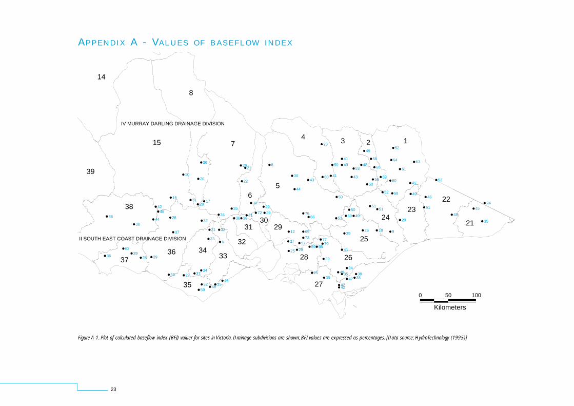
AP P E N D I X A - VA L U E S O F B A S E F L O W I N D E X

Figure A-1. Plot of calculated baseflow index (BFI) valuer for sites in Victoria. Drainage subdivisions are shown; BFI values are expressed as percentages. [Data source; HydroTechnology (1995)]

39

14

37

38

II SOUTH EAST COAST DRAINAGE DIVISION

36

15

IV MURRAY DARLING DRAINAGE DIVISION

8

34

35

7

36

1020

4842

16

26

37

28 2939

62

36

38

36

34

59

3727

32

31

33

3029

12

236

32

173128

4635

4552

65

3221

3436

30

72 2936

31

35

21

22

626

28

27

73

69

57

29

27

25

76

44

30

29

38

26

0 50

34

39

3538

49

4239

4242

3925

2541

7059 65

77

66

391826

51

50

43

Kilometers

100

2423

21

22

9

29

4524

35

48

46

61

52

49

49

45

61

5852

5151

50

50

63

4 3 2 1

596056

50

60

64

52

58

49

43

4853

49

41

50

23

4160

44

A cooperative venture between:Bureau of MeteorologyCSIRO Land and WaterDepartment of Natural Resources andEnvironment, VicGoulburn-Murray WaterMelbourne WaterMonash UniversityMurray-Darling Basin CommissionSouthern Rural WaterThe University of MelbourneWimmera-Mallee Water

Associates:Department of Land and WaterConservation, NSWDepartment of Natural Resources, QldHydro-Electric Corporation, TasState Forests of NSW

Centre OfficeDepartment of Civil Engineering

Monash UniversityClayton, Victoria 3168 Australia

http://www-civil.eng.monash.edu.au/centres/crcch/

Established and supported under the Australian Government’s Cooperative

Research Centres Program