DI

SC

US

SI

ON

P

AP

ER

S

ER

IE

S

Forschungsinstitut zur Zukunft der ArbeitInstitute for the Study of Labor

Education and Optimal Dynamic Taxation

IZA DP No. 6056

October 2011

Sebastian FindeisenDominik Sachs

Education and

Optimal Dynamic Taxation

Sebastian Findeisen University of Zurich

and IZA

Dominik Sachs University of Konstanz

Discussion Paper No. 6056 October 2011

IZA

P.O. Box 7240 53072 Bonn

Germany

Phone: +49-228-3894-0 Fax: +49-228-3894-180

E-mail: iza@iza.org

Any opinions expressed here are those of the author(s) and not those of IZA. Research published in this series may include views on policy, but the institute itself takes no institutional policy positions. The Institute for the Study of Labor (IZA) in Bonn is a local and virtual international research center and a place of communication between science, politics and business. IZA is an independent nonprofit organization supported by Deutsche Post Foundation. The center is associated with the University of Bonn and offers a stimulating research environment through its international network, workshops and conferences, data service, project support, research visits and doctoral program. IZA engages in (i) original and internationally competitive research in all fields of labor economics, (ii) development of policy concepts, and (iii) dissemination of research results and concepts to the interested public. IZA Discussion Papers often represent preliminary work and are circulated to encourage discussion. Citation of such a paper should account for its provisional character. A revised version may be available directly from the author.

IZA Discussion Paper No. 6056 October 2011

ABSTRACT

Education and Optimal Dynamic Taxation* We study optimal tax and educational policies in a dynamic private information economy, in which ex-ante heterogeneous individuals make an educational investment early in their life and face a stochastic wage distribution. We characterize labor and education wedges in this setting analytically and numerically, using a calibrated example. We present ways to implement the optimum. In one implementation there is a common labor income tax schedule, and a repayment schedule for government loans given out to agents during education. These repayment plans are contingent on loan size and income and capture the history dependence of the labor wedges. Applying the model to US-data and a binary education decision (graduating from college or not) we characterize optimal labor wedges for individuals without college degree and with college degree. The labor wedge of college graduates as a function of income lies first strictly above their counterparts from high-school, but this reverses at higher incomes. The loan repayment schedule is hump-shaped in income for college graduates. JEL Classification: H21, H23, I21 Keywords: optimal dynamic taxation, education, implementation Corresponding author: Sebastian Findeisen University of Zurich Department of Economics Muehlebachstr. 86 8008 Zurich Switzerland E-mail: sebastian.findeisen@uzh.ch

* We thank Dan Anderberg, Friedrich Breyer, Carlos da Costa, Mike Golosov, Florian Scheuer, Dirk Schindler, Kjetil Storesletten, Iván Werning, Christoph Winter, Fabrizio Zilibotti, and seminar participants in Bloomington, Gerzensee, Konstanz, Stanford, Yale and Zurich for helpful comments. We also thank Stefan Voigt for valuable research assistance.

1 Introduction

A well-established link exists between income inequality and education. In a recentsurvey Acemoglu and Autor (2010) note that the college premium has been risingsteadily in the US for the last 45 years with no immediate end in sight. This wideningwage premium has contributed to an increase in the dispersion of the distributionof wages and income also in other advanced economies (Krueger, Perri, Pistaferriand Violante 2010). However, not all of the observed rise in the college premium isnecessarily caused by an increased demand for skills acquired in college to the extentthat unobserved skills influence wages and labor market outcomes in general. Taber(2001) finds that at least some of the observed rise in the educational skill premiumshould be attributed to unobserved skill heterogeneity realized before college decisionsare made.1 Furthermore, since heterogeneity is already realized at a very early stagein life, individuals face very different returns to education, resulting in very differentincentives to invest into education2 Finally, it is well known that returns to educationare subject to substantial uncertainty.3

What are the implications of these empirical relationships for optimal policies?How can non-linear labor taxes be used to dampen inequality? Should informationabout one’s education level be included in the tax code? How should education poli-cies be set and how are incentives to invest into human capital affected by the taxcode for ex-ante heterogeneous agents? What role do policies have to insure risk?

In this paper, we try to make progress on these important questions in a norma-tive Mirrleesian framework, using both theory and numerical simulations. Althoughprevious papers have studied optimal taxation problems with endogenous educa-tion, they have typically abstracted from either ex-ante heterogeneity or uncertainty,or imposed exogenous restrictions on the available policy instruments (e.g. only lin-ear taxes). To address this issue, we build a more realistic setting including bothex-ante heterogeneity and uncertainty in educational returns. In addition, the set ofpolicy instruments is endogenous, arising solely from the informational structure ofthe problem.

More formally, we study an environment characterized by private information,which evolves stochastically over time. Ex-ante heterogeneous individuals are bornwith different innate abilities θ and decide on their level of education z early in theirlife. After education, agents learn their skill level a that can be interpreted as wage,

1Indirect evidence for the importance of unobserved skills comes from the strong persistence ofwithin education group inequality.

2See, for example, Lemieux (2006) or Carniero and Heckman (2003). We give a brief review of keyempirical findings guiding our modeling later in the paper.

3See, e.g., Cunha, Heckman and Navarro (2005).

2

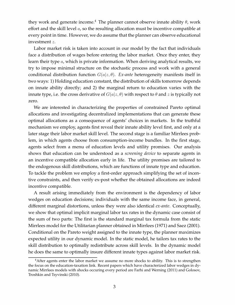
they work and generate income.4 The planner cannot observe innate ability θ, workeffort and the skill level a, so the resulting allocation must be incentive compatible atevery point in time. However, we do assume that the planner can observe educationalinvestment z.

Labor market risk is taken into account in our model by the fact that individualsface a distribution of wages before entering the labor market. Once they enter, theylearn their type a, which is private information. When deriving analytical results, wetry to impose minimal structure on the stochastic process and work with a generalconditional distribution function G(a|z, θ). Ex-ante heterogeneity manifests itself intwo ways: 1) Holding education constant, the distribution of skills tomorrow dependson innate ability directly; and 2) the marginal return to education varies with theinnate type, i.e. the cross derivative of G(a|z, θ) with respect to θ and z is typically notzero.

We are interested in characterizing the properties of constrained Pareto optimalallocations and investigating decentralized implementations that can generate theseoptimal allocations as a consequence of agents’ choices in markets. In the truthfulmechanism we employ, agents first reveal their innate ability level first, and only at alater stage their labor market skill level. The second stage is a familiar Mirrlees prob-lem, in which agents choose from consumption-income bundles. In the first stage,agents select from a menu of education levels and utility promises. Our analysisshows that education can be understood as a screening device to separate agents inan incentive compatible allocation early in life. The utility promises are tailored tothe endogenous skill distributions, which are functions of innate type and education.To tackle the problem we employ a first-order approach simplifying the set of incen-tive constraints, and then verify ex-post whether the obtained allocations are indeedincentive compatible.

A result arising immediately from the environment is the dependency of laborwedges on education decisions; individuals with the same income face, in general,different marginal distortions, unless they were also identical ex-ante. Conceptually,we show that optimal implicit marginal labor tax rates in the dynamic case consist ofthe sum of two parts: The first is the standard marginal tax formula from the staticMirrlees model for the Utilitarian planner obtained in Mirrlees (1971) and Saez (2001).Conditional on the Pareto weight assigned to the innate type, the planner maximizesexpected utility in our dynamic model. In the static model, he tailors tax rates to theskill distribution to optimally redistribute across skill levels. In the dynamic modelhe does the same to optimally insure different innate types against labor market risk.

4After agents enter the labor market we assume no more shocks to ability. This is to strengthenthe focus on the education-taxation link. Recent papers which have characterized labor wedges in dy-namic Mirrlees models with shocks occuring every period are Farhi and Werning (2011) and Golosov,Troshkin and Tsyvinski (2010).

3

Since the endogenous skill distribution is different for each innate type, there is oneinsurance part of labor taxation for every initial type. For the second effect and to fixideas, consider the case of only two innate types θL and θH . We show that the marginaltax rate at some income level y(a∗) for the low type θL depends positively on to thedifference: (1−G(a∗|z, θH))− (1−G(a∗|z, θL)) = Pr(a > a∗|z, θH)− Pr(a > a∗|z, θL).To look at a specific example, let us consider a first-order stochastic dominance order-ing of the type spaceG(a|z, θH) �FOSD G(a|z, θL), so the above term is never negative.The planner increases the marginal distortion for the low type proportional to the dif-ference in order to deter a deviation from high types, who have a higher likelihoodof being a higher type than a∗ and therefore of being affected by this higher marginaldistortion through a decrease in consumption. Differences in the conditional distri-bution are exploited in this way by the planner to effectively deal with the incentiveconstraints in the first period

The dependency of the tax schedules on characteristics other than income is re-lated to the idea of tagging and income taxation, as first proposed by Akerlof (1978).5

Whereas our analysis shares the feature of this method in that the social planner usesadditional information to tailor marginal tax rates for each educational level to therespective skill distribution, it differs substantially in the sense that education is notan immutable tag, but rather an endogenous variable. One might, therefore, label thedependency of tax distortions on education as endogenous tagging.6

Our theory illustrates how individual education decisions are distorted by optimalgovernment intervention in constrained Pareto optimal allocations. This dependsagain on two forces. First, implicit educational subsidies are used to offset the dis-tortionary impact of the labor tax on educational decisions. This is equivalent to afirst-best rule in a sense that innate ability would be observable. Second, the plannerdistorts education to relax binding incentive constraints. If the desired redistributionof income is downward (high to low innate types), we show that this imposes an im-plicit tax and hence a downward distortion of education. The key is that this improvesthe equity-efficiency trade-off for the planner, in the same spirit as positive marginallabor tax rates relax incentive constraints in the static model.

We numerically illustrate these forces, parameterizing the skill distributions as log-normal with a Pareto tail, following standard practice in the literature. We set thelocation parameter of the log-normal to be a function of innate skills and education,allowing for differing marginal returns to education across agents. We discipline ourparameter choice by matching monetary education expenditures on college educationin the US. Holding income constant, implicit marginal tax rates on labor income differ

5More recently tagging is investigated by Cremer, Gahvari and Lozachmeur (2010), Mankiw andWeinzierl (2010) as well as Weinzierl (2011b).

6A similar logic arises in the recent paper of Scheuer (2011) in a model with endogenous occupa-tional choices.

4

by up to 21 % points across different education levels in our numerical example. Thesedifferences are mainly explained by tailoring marginal tax rates to the different skilldistributions. We find only small second-order effects of the dynamic incentive effectdescribed above. For the education wedge we find that it is mainly determined bythe first-best rule and that the downward distortion to relax incentive constraints isof minor magnitude.

We propose two ways to decentralize the optimum. In one implementation, thegovernment offers a non-linear schedule of grants to individuals. These grants arelinked to education levels. Agents self-select into education and use the grants to fi-nance tuition and consumption during education. After graduating they are free tochoose their work hours/effort and pay a labor income tax conditioning on their ed-ucation choice. Together with a savings tax these polices can achieve the optimum.Such history dependent tax schedules might be considered hard to implement in prac-tice, since they might be perceived as violating horizontal equity by society. Dealingwith that, we provide another implementation that is basically a reinterpretation ofthe first one: Agents are offered loans during their education period that are linkedto education levels. When working, all individuals face the same history - indepen-

dent tax schedule and in addition a loan repayment schedule that depends both onincome and on the size of the loan.7 Since the government effectively provides liquid-ity to agents during their education, both implementation would also be applicable ifagents were credit constrained.

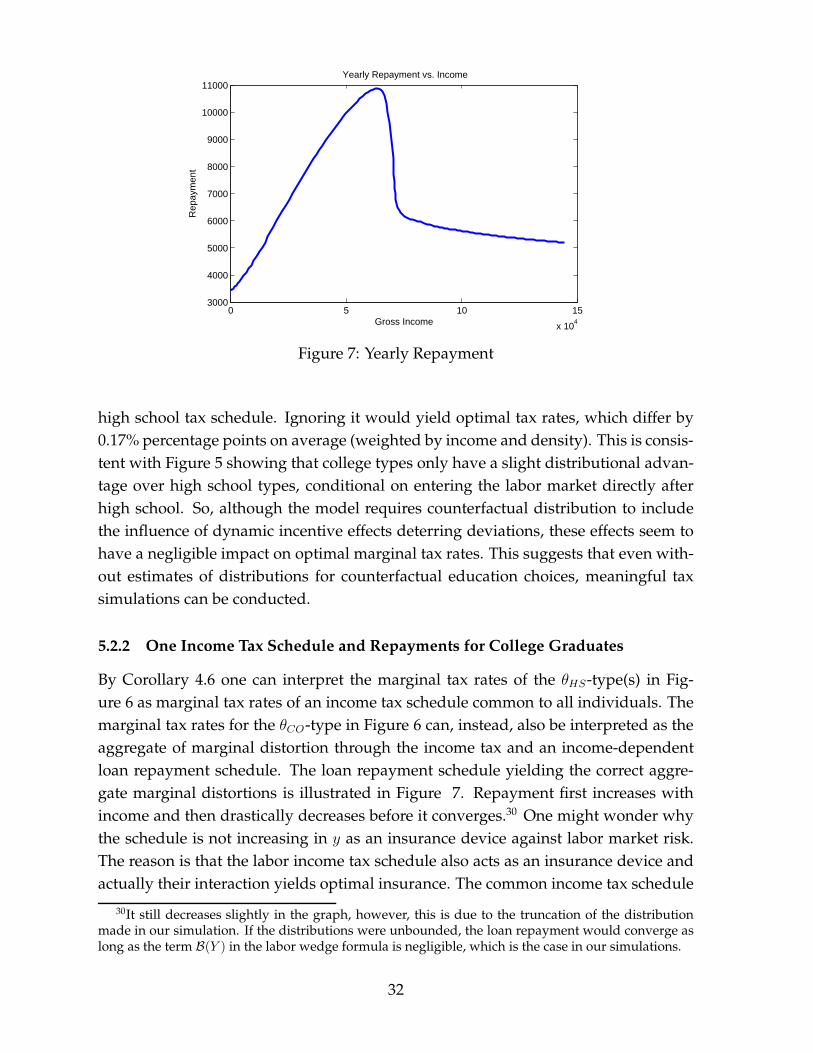
Finally, we present a simpler application of the model, using a binary educationdecision, i.e. going to college or not. Importantly, this enables us to use estimatesof factual as well as counterfactual income distributions from the labor economicsliterature (Cunha and Heckman 2007, 2008), both of which are needed as an inputto the model. Additionally, by reducing the dimensionality of the problem, a binaryeducation choice also significantly reduces the complexity and sophistication of thepolicy instruments, coming another step closer to practical policy recommendations.For high-school and college graduates optimal implicit labor tax rates are both U-shaped as in Diamond (1998) and Saez (2001). Marginal tax rates for college graduatesare first higher then smaller, before both schedules converge to roughly the same toptax rate. Using the high-school labor wedge schedule as the common labor income taxschedule, the implied income-contingent repayment schedule for college graduates ishump-shaped. In expectation college graduates pay a small yearly premium over theactuarially-fair annuity value of the loan they take from the government.

Related Literature. Several previous papers have studied problems of optimallabor taxation and their relation to education decisions. One strand of inquiry has

7Income-contingent loan repayments are actually in place in Australia, Great Britain, Sweden, Nor-way and New Zealand.

5

worked under the assumption of ex-ante homogeneity and risky human capital. Grochul-ski and Piskorski (2010) focus on the implications of unobservable human capital in-vestment for capital taxation. Anderberg (2009) emphasizes that the risk propertiesof human capital are crucial for the question whether and how education should bedistorted relative to a first-best rule.8 Da Costa and Maestri (2007) show that humancapital should always be encouraged in a second-best environment. In contrast, ourmodel explicitly stresses the importance of heterogeneity, already at the point wheneducation decisions are made.

In a static setting with heterogeneity but without uncertainty, Bovenberg and Ja-cobs (2005) analyze how endogenous education alters the result of the Mirrleesian taxproblem and conclude that distortions on the education margin through income tax-ation should be offset by education subsidies. Relatedly, Bohacek and Kapicka (2008)study a model in a dynamic environment with certainty and obtain similar results.9

Some of the mentioned papers analyze unobservable human capital investment andsome the observable case. Which assumption is appropriate depends on the exact re-search question since in reality some parts of human capital are observable (type ofdegree, student fees, years at college) and some parts are not (e.g. study behavior).One aim of our paper is to argue that in an social optimum, using available publicinformation about human capital can act as a screening device; that is why we focuson modeling the observable part of human capital investment.

Bénabou (2002) considers the case of heterogeneity and uncertainty. His approachis different from ours in two ways: first, he does not solve for constrained Paretooptimal allocations, but instead focuses on given non-linear instruments: educationsubsidies and income taxes. Second, he does not consider the optimum using bothinstruments simultaneously, but rather compares the implications of education subsi-dies with those of progressive income taxes for growth and efficiency. Our approachis to derive the full optimum constrained only by informational asymmetries andthen discuss policy instruments implementing these allocations in line with the NewDynamic Public Finance literature.

Two recent contributions have analyzed optimal labor wedges in dynamic Mirrleeseconomies without endogenous education but with productivity shocks in every pe-riod, which we abstract from. Farhi and Werning (2011) characterize the evolution ofthe labor wedge over time analytically and numerically. Golosov, Troshkin and Tsyvin-ski (2010) derive and illustrate optimal labor wedges across agents in the case of no

8Focusing on linear policy instruments Anderberg and Andersson (2003) as well as Jacobs,Schindler and Yang (2010) also discuss the importance of the risk properties of human capital.

9Kapicka (2006) introduces non-observable endogenous human capital into a dynamic, non-stochastic Mirrlees model where taxes can only be conditioned on current income. He shows thatmarginal tax rates are lowered due to the education margin. Bovenberg and Jacobs (2005) considerobservable and unobservable investment and provide an interesting discussion about different impli-cations.

6

income effects and non-separable preferences. Our analysis on labor wedges focuseson differences across education levels in an optimal allocation and is, therefore, com-plementary.

To make the dynamic incentive problem tractable, we employ a first-order ap-proach. Importantly, we rely on the fact that private information evolves sequentiallyin our economy, which avoids solving a multidimensional screening problem. Thispaper is, thus, related to work on dynamic mechanisms, in particular that of Pavan,Segal and Toikka (2011) and Kapicka (2010), who study the validity and robustness ofthe Mirrleesian first-order approach in dynamic economies, as well as that of Courtyand Li (2000) who study optimal dynamic pricing of a monopolist.

Finally our paper builds on recent important work by Werning (2011), who showsthat decentralized implementations of incentive compatible allocations, which arecharacterized by non-stochastic, non-linear capital taxes that may even be history in-dependent, do exist.

This paper is organized as follows. Section 2 contains the basics of the model aswell as its empirical foundation and a short characterization of the Laissez-Faire allo-cation. In Section 3, we investigate dynamic incentive compatibility and describe themajor properties of constrained efficient allocations. Further on, we present quantita-tive results with a calibrated example. Decentralized implementations of constrainedefficient allocations are provided in Section 4. Using data from Cunha and Heckman(2007, 2008) we apply our model to the case of a binary education decision in Section5. Section 6 concludes.

2 Baseline Model

2.1 Heterogeneity, Education and Labor Market Outcomes: Some

Empirical Facts

We begin with a brief discussion of recent evidence and stylized facts from the em-pirical literature on education and labor market outcomes and state how these guideour modeling assumptions. These findings underscore the importance of the effectof initial heterogeneity and risk on the returns to education. A series of papers haveused factor structure models to estimate returns to education (see Cunha and Heck-man (2007) for a survey). Importantly, these methods can identify whole distributionsof returns (instead of first and second moments only), do counterfactual analysis, anddistinguish between ex-ante and ex-post returns.

First, Cunha and Heckman (2008) document considerable residual uncertainty overfuture returns at the time of the decision to go to college or enter the labor market di-rectly after high school, even after controlling for heterogeneity.

7

Second, for both groups, actual college and high-school graduates, the density oflifetime earnings when going to college, lies to the right of the density when enteringthe labor after high school indicating a first-order stochastic dominance shift. Notethat for high-school graduates the college density is estimated counterfactually andvice-versa for college graduates.

Third, returns to education differ widely across individuals. Carniero and Heck-man (2003) document that the return can differ by as much 19% points across indi-viduals for one year of college. In this vein, the literature has documented a com-plementarity effect – both cognitive and non-cognitive ability, either acquired earlyduring childhood or innate, increase the return of education. For example, Altonjiand Dunn (1996) find that the return is higher for children whose parents are highlyeducated; these parents are likely to be more able to transmit or instill their offspringwith higher initial human capital. Finally, there is evidence of a direct effect of theseearly abilities on earnings. Taber (2001) presents findings suggesting that much of therise in the college premium may be attributed to a rise in the demand for unobservedskills, which are predetermined and independent of education.

2.2 The Model

Individuals, whose mass is normalized to one, live for two periods. In the first periodindividuals acquire human capital and in the second period individuals work. Thelabor market ability in period two, however, is stochastic in period one. The distribu-tion of labor market abilities depends on educational investment and initial type. Wenow formalize these ideas.

In period one individuals differ in innate ability θ, which can be interpreted asa one dimensional aggregate of (non-)cognitive skills and family background and isdistributed in the interval [θ, θ] according to F (θ). When individuals learn their typeθ, which is private information, they make an educational investment. z10

In period two individuals draw their labor market ability a from a continuous con-ditional distribution G(a|z, θ), which depends on innate ability θ and education z, andhas bounded support [a, a]. When individuals learn their type a they make a labor-leisure decision.

To sharpen a few analytical results, it turns out helpful to place some structure onthe behavior of G(a|z, θ):

Assumption 1: G(a|z′, θ) �FOSD G(a|z, θ) ⇔ G(a|z′, θ) ≤ G(a|z, θ), for all z < z′.

10Reducing education to a one-dimensional, monetary variable is admittedly a simplification ofreality. Nevertheless, we think it is reasonable to downsize the complex education process like thissince it captures the important fact that more education always requires more resources and makes theanalysis tractable.

8

Assumption 2: G(a|z, θ′) �FOSD G(a|z, θ) ⇔ G(a|z, θ′) ≤ G(a|z, θ), for all θ < θ′.

Assumption 3: ∂2G(a|z,θ)∂θ∂z

≤ 0.

These assumption will not be needed to derive our main results, but help to il-lustrate important aspects of the model. Whenever an assumption is needed for aresult, we refer to it. The first and the second one capture the notion that educationand the innate ability level should both have a direct effect on labor market outcomesrepresented by a first-order stochastic dominance shift. The third one captures theirinteraction and respects the compelling evidence of complementarity between earlyability and education.

2.3 Laissez Faire Equilibrium

To lay out the basic properties of the model, we start with the characterization ofthe government intervention free laissez-faire equilibrium. In the second period, af-ter agents have learned their labor market skill a, they choose labor supply, takingsavings or private debt as given. This gives rise to the indirect utility function:

v2(a, s(θ)) = maxy,c2

u (c2)−Ψ(y

a

)

s.t. c2 = y +Rs(θ).

Individuals’ utility functions are well-behaved – u(.) is assumed to be increasing, atleast twice continuously differentiable and concave, and Ψ(.) is assumed to be in-creasing, at least twice continuously differentiable and convex. The parameter a is anindividual’s labor market skill, meaning individuals with a higher a need to provideless labor effort to earn any income y.

In the first period, agents decide how much to invest into education, and makea consumption-saving decision. Agents have access to a risk-free one period bondmarket; we impose no short-sale or enforcement constraints and an exogenous grossreturn R. This defines the indirect utility function:

V (θ) = maxs,z,c1

u(c1) + β

∫ a

a

v2(a, s)g(a|z, θ)da s.t. c1 + z = −s.

As already anticipated in the last Section, we model the conditional distribution ofskills g(a|z, θ) as being determined by an agent’s education level z and her innateability θ. Moreover, we focus on educational investment as a direct monetary cost.This is consistent with the idea that tuition fees and other monetary expenses are themost important factors on the cost side driving educational decisions. It is also in linewith a foregone earnings interpretation, where more education delays labor marketentry. z can be a sum of both factors. In our numerical simulations in Section 5 we

9

explicitly allow for the fact that different levels of education last a different numberof periods.

We now present the main properties of the equilibrium without government poli-cies:

Proposition 2.1. The Laissez-Faire allocation has the following properties:

(i) The Euler Equation holds:

u′(c1(θ)) = βR∫ a

au′(c2(θ, a))dG(a|z(θ), θ)

(ii) Labor supply is undistorted: Ψ′(

y(θ,a)a

)

1a= u′(c2(θ)).

(iii) The marginal cost of education is equalized to marginal benefits:

u′(c1(θ)) = β∫ a

av2(θ, a)

∂g(a|z(θ),θ)∂z

da

(iv) If Assumptions 1-3 hold, educational investment is increasing in innate ability and sav-

ings are decreasing, i.e. z′(θ) > 0 and s′(θ) < 0.

Proof. See Appendix A.1

Parts (i)-(iii) follow directly from the first-order conditions. They are unsurprisingproperties, stating that private marginal rates of substitution are equated to technicalmarginal rates of transformation on the labor, capital, and education market.

Part (iv) states that without government policies, education and savings are mono-tone in innate ability θ if Assumptions 1-3 are fulfilled. The proof provides instructiveintuition for this result. It is sufficient to show that the objective defined by (2.3) issupermodular in all choice variables and type θ (see Milgrom and Shannon (1994)).Plugging in the budget constraint gives the problem reduced to two choices s and z:maxs,z U(s, z; θ, a, β) = u(−s− z)+β

∫ a

av2(a, s)g(a|z, θ)da. This objective is supermod-

ular in credit taken −s, education z and type if and only if:

∂2U(s, z; θ, .)

∂s∂θ< 0 (1)

∂2U(s, z; θ, .)

∂s∂z< 0 (2)

∂2U(s, z; θ, .)

∂z∂θ> 0. (3)

In Appendix A.1 we show that all inequalities hold. Equations (1) and (2) imply thatthe return to savings is lower for higher θ types and with higher education, sinceexpected labor skills are also higher. Equation (3) holds, since innate abilities and ed-ucation are complementary to each other. Taken together the direct effects of being ofhigher type on credit and education are being reinforced by the relationship betweenthe endogenous variables.

So far, we have assumed no limits on the ability of agents to borrow against futurelabor income. Imposing an ad-hoc constraint of the form s ≥ φ, where φ is some neg-

10

ative number, leaves most of the results from Proposition 2.1 unaffected.11 Notably,constrained agents will not be able to smooth consumption intertemporally as muchas desired. Still education levels will be increasing in type:

Corollary 2.2. Suppose Assumptions 1 to 3 hold. If agents face borrowing constraints s ≥ φ,

education is still monotone in type θ, i.e. z′(θ) > 0 in the laissez-faire equilibrium.

Proof. Above some threshold type, agents reach the borrowing limit and set s equalto φ. Of those agents higher types still face the greater returns to education becauseof the complementarity and therefore choose a higher level of z.

The empirical literature has also documented sorting into education, based on het-erogeneous expected returns (Cunha and Heckman 2007). The monotonicity of edu-cation in the laissez-faire equilibrium is consistent with that fact.

For later purposes when we analyze optimal allocations and the respective tax sys-tems that can implement such allocations, it is useful to define three wedges. Theyare equal to implicit marginal tax rates on savings, labor income and education, re-spectively:

Savings wedge:

τs(θ) = 1−u′(c1(θ))

βR∫ a

au′(c2(θ, a))g(a|z, θ)da

Importantly, like all wedges the intertemporal wedge is defined for any given allo-cation. It is the proportional adjustment needed in the rate of return to make theEuler equation hold for an agent θ, given the particular allocation. It follows that inany allocation, there are as many wedges as agents – one for each innate skill level.τs(θ) > (<)0 implies a downward (upward) distortion of savings. The same is truefor the following wedge.

Labor wedge: The labor wedge is nonzero if an individual would like to work more orless at the intervention-free market price (which is her productivity level a). Formallythe labor wedge reads as:

τy(θ, a) = 1−Ψ′

(

y(θ,a)a

)

1a

u′(c2(θ, a))

It again has to be evaluated for a given allocation and there exists exactly one laborwedge for every type vector (θ, a).

11Surveying the literature, Carniero and Heckman (2003) conclude that short-term borrowing con-straints seem to have only a very small effect on educational decisions.

11

Educational wedge: The education wedge is nonzero if the individual wants to ob-tain more or less education if it could do that at the market price z. Formally it readsas

τz(θ) = 1−β∫ a

av2(θ, a)

∂g(a|z(θ),θ)∂z(θ)

da

u′(c1(θ)).

In this case, a positive wedge corresponds to an upward distortion of education.In the decentralized systems we later propose for the implementation of constrained

Pareto efficient allocations, we will show, which of these implicit taxes on labor income,savings and education will equal explicit marginal taxes

3 Constrained Pareto Optimal Allocations

In this Section we characterize constrained Pareto efficient allocations, where ’con-strained’ refers to the government being unable to observe agents’ type θ in periodone and a in period two. In Subsection 3.1, we show that the problem is tractableusing a first-order approach. In addition we provide necessary as well as sufficientconditions for this approach to be valid. In Subsection 3.2, we analyze optimality con-ditions and its consequences for optimal policies. In Subsection 3.3, we show how theresults are extended to a T -period framework and in Subsection 3.4, we explore theimplications for optimal policies using numerical simulations.

3.1 Incentive Compatibility

We cast the problem as a sequential, dynamic mechanism – agents report an initialtype θ in the first period, and, after uncertainty has materialized, report their produc-tivity a in the second period. The planner assigns initial consumption levels c1(θ) andeducation levels z(θ) to individuals with innate ability θ. Moreover, with each reportthere comes a sequence of utility promises for the next period {v2(θ, a)}a∈[a,a]. In thesecond period the screening takes place over consumption levels c2(θ, a) and laborsupply y(θ, a). All these quantities define an allocation in the economy. Dynamic in-centive compatibility is ensured backwards, so we start analyzing the problem fromthe second period.12

3.1.1 Second Period Incentive Compatibility

By the revelation principle, we can restrict attention to direct mechanisms. Supposein the first period agents have made truthful reports r(θ) = θ, although this is not

12A similar first-order approach can be readily applied int the case of a discrete choice for education;i.e. the planner deciding which agents to send to college and which not. Incentive compatibility hasthen to be characterized using modified envelope theorems in the spirit of Milgrom and Segal (2002).

12

necessary and just simplifies the exposition. Conditions for this to be true are givenin the next Section. Conditional on this report, the second period incentive constraintmust be met for any history of types (θ, a) and reporting strategy r(a):

u (c2 (θ, a))−Ψ

[

y(θ, a)

a

]

≥ u (c2 (θ, r(a)))−Ψ

[

y(θ, r(a))

a

]

∀a, r(a).

Define the associated indirect utility function of the agents as:

v2(θ, a) = maxr(a)

u (c2 (θ, r(a)))−Ψ

[

y(θ, r(a))

a

]

.

Like in a standard Mirrleesian problem preferences satisfy single-crossing for givenfirst-period reports. For global incentive compatibility it is, hence, necessary and suf-ficient that all local envelope conditions hold:

∂v2(θ, a)

∂a= Ψ′

(

y(θ, a)

a

)

y(θ, a)

a2, (4)

and the usual monotonicity condition, stating that y(θ, a) is non-decreasing in abilitylevels a, is satisfied:

∂y(θ, a)

∂a≥ 0

3.1.2 First Period Incentive Compatibility

Importantly, in the first period an agent takes into account the effect of her reportabout θ on future utility. First period incentive compatibility is ensured if and only ifthe double continuum of weak inequalities holds:

U(θ, θ) = u (c1 (θ)) + β

∫ a

a

v2(θ, a)dG(a|z(θ), θ)

≥u (c1 (r(θ))) + β

∫ a

a

v2(r(θ), a)dG(a|z(r(θ)), θ) = U(θ, r(θ)), ∀θ, r(θ), (5)

where U(θ, r(θ)) is the expected utility of an individual of type θ reporting r(θ). Theassociated value function is:

V (θ) = maxr(θ)

u (c1 (r(θ))) + β

∫ a

a

v2(r(θ), a)dG(a|z(r(θ)), θ).

13

We proceed by replacing the set of inequality constraints defined by (5) by local enve-lope conditions analogous to the ones for the second period:

dV (θ)

dθ= β

∫ a

a

v2(θ, a)∂g(a|z(θ), θ)

∂θda. (6)

Innate ability affects the indirect utility function directly through the serial corre-lation in types only. This localization of incentive constraints to make the problemtractable is only valid if they imply a maximum from the point of view of the agentsfor a truthful report and also imply global incentive compatibility. We now proceed bycharacterizing necessary conditions for local and then global incentive compatibility.The first-order condition for an optimal report, evaluated at the revealing strategy,must obey:

∂U(θ, θ)

∂r(θ)= 0. (7)

For a local maximum it is necessary that:

∂2U(θ, θ)

∂r(θ)2≤ 0.

Differentiating equation (7) yields:

∂2U(θ, θ)

∂r(θ)2+∂2U(θ, θ)

∂r(θ)∂θ= 0.

In any incentive compatible allocation it must, hence, hold that:

∂2U(θ, θ)

∂r(θ)∂θ=

∫ a

a

∂v2(θ, a)

∂θ

∂g(a|z(θ), θ)

∂θda+

∂z(θ)

∂θ

∫ a

a

v2(θ, a)∂2g(a|z(θ), θ)

∂z∂θda ≥ 0.

We summarize these findings in the following Lemma:

Lemma 3.1. An allocation is incentive compatible only if:

(i)dV (θ)dθ

= β∫ a

av2(θ, a)

∂g(a|z(θ),θ)∂θ

da

(ii)∂2U(θ,θ)∂r(θ)∂θ

=∫ a

a∂v2(θ,a)

∂θ∂g(a|z(θ),θ)

∂θda+ ∂z(θ)

∂θ

∫ a

av2(θ, a)

∂g(a|z(θ),θ)∂z∂θ

da ≥ 0,

(iii) ∂v2(θ,a)∂a

= Ψ′(

y(θ,a)a

)

y(θ,a)a2

,

(iv) ∂y(θ,a)∂a

≥ 0.

This Lemma provides necessary or localized conditions for any incentive compat-ible allocation. Its first part (i) can be conveniently included into any Lagrangian oroptimal control problem. Part (ii) can be interpreted as follows: ∂2U(θ,θ)

∂r(θ)∂θ≥ 0 holds if

the initial type θ and the report r are complements. The expression can be decom-posed into two terms. The first term captures the idea that promised utilities should

14

be tailored to different distributions of different initial types; roughly spoken higherinitial types should have relatively higher promised utilities in better states. The sec-ond term enters this condition due to the endogenous investment z(θ) and capturesthe idea that individuals with higher returns to education should receive a higherlevel of education. Parts (iii) and (iv) are the well-known envelope and monotonicitycondition from the static Mirrlees problem, holding the innate type θ constant. Likein the standard problem parts (iii) and (iv) are necessary and sufficient, which can beshown by a standard proof.

As often done in screening problems, our strategy for solving the second-best prob-lem is to work with a relaxed problem with only restrictions (4) and (6) being imposedand then check ex-post whether incentive compatibility is fulfilled. In the numericalexplorations in Section 3.4 we find that incentive compatibility is always satisfied andtherefore the first-order approach is valid for the considered primitives.

We now present a result that is interesting especially from a theoretical point ofview.

Lemma 3.2. Suppose Assumptions 2 and 3 hold, and conditions (i), (iii), (iv) of Lemma 3.1

are satisfied and further we have:

(i)∂y(θ,a)∂θ

> 0,

(ii)∂z(θ)∂θ

> 0,

then the considered allocation is incentive compatible.

Proof. See Appendix A.2.

This Lemma implies that instead of directly ex-post verifying whether period oneincentive compatibility is satisfied in an allocation, one can alternatively check thesetwo simple monotonicity conditions. If they are fulfilled, then the allocation is in-centive compatible. However, for both to be fulfilled is sufficient and not necessary.Whereas condition (ii) was always fulfilled in our numerical examples, condition (i)

often was violated for low a; we will comment on the reasons in Section 3.4 when wepresent numerical illustrations of the model.

Our results on dynamic incentive compatibility are related to previous work in theoptimal non-linear pricing literature by Courty and Li (2000). They study optimalpricing schemes of a monopolist facing consumers with stochastic tastes. In our casethe distribution of types tomorrow is endogenous, since education is a choice. Inrecent contributions, Kapicka (2010) as well as Pavan, Segal and Toikka (2011) inves-tigate the robustness and validity of the Mirrleesian first-order approach in a largeclass of general dynamic environments.

15

3.2 Characterization

The planner maximizes

∫ θ

θ

u(c1(θ))dF (θ) + β

∫ θ

θ

∫ a

a

v2(θ, a)dG(a|z(θ), θ)dF (θ)

subject to (4), (6) and the resource constraint:

∫ θ

θ

[

c1(θ)− z(θ) +1

R

∫ a

a

(c2(θ, a)− y(θ, a))dG(a|z(θ), θ)

]

dF (θ) = 0

where R is the gross return on savings. We let the planner assign Pareto weightsF (θ) to individuals, depending (solely) on their initial skill level. Any distribution of

these weights, which we normalize to satisfy∫ θ

θf(θ)dθ = 1, corresponds to one point

on he Pareto frontier. λR denotes the multipliers on the resource constraint and η(θ)

the multiplier function of the first-period envelope conditions. In Appendix A.3 theLagrangian and the first-order conditions of the problem are stated. We now charac-terize the wedges of second-best allocations.

3.2.1 Savings Distortions

It turns out that the presence of education, which endogenously affects the probabil-ity distribution of tomorrow’s skills, does not change the prescription of a positiveintertemporal wedge, stemming from the optimality of the Inverse Euler equationin dynamic Mirrleesian models.13 Some manipulations of the first-order conditionsyield the following proposition:

Proposition 3.3. In any constrained Pareto optimum, the inverse Euler equation holds:

1

u′(c1(θ))=

1

βR

∫ a

a

1

u′(c2(θ, a))g(a|z(θ), θ)da =

1

βREa|θ

[

1

u′(c2(θ, a))

]

.

Proof. See Appendix A.4.1.

Jensen’s inequality then implies βE [u′(c2(θ, a))] > u′(c1(θ)) – the optimal allocationdictates a wedge between the intertemporal rate of substitution and transformation;savings are discouraged.

13Diamond and Mirrlees (1978) and Rogerson (1985) were the first to derive it. In an importantpaper reviving the interest in the result, Golosov, Kocherlakota and Tsyvinski (2003) generalized it toa large class of dynamic environments, most importantly allowing for arbitrary skill processes. Muchlike the Atkinson and Stiglitz (1976) prescription of uniform commodity taxes, the robustness of apositive intertemporal wedge relies on the (weak) separability of consumption and work effort.

16

3.2.2 Labor Distortions

The following proposition characterizes the optimal labor wedge.14

Proposition 3.4. At any constrained Pareto optimum, labor wedges satisfy:

τy(θ, a)

1− τy(θ, a)=

1 + εu(θ, a)

εc(θ, a)

u′(c2(θ, a))

ag(a|z(θ), θ)[A(θ, a) + B(θ, a)] ,

where

A(θ, a) =G(a|z(θ), θ)

[

∫ a

a

1

u′(c2(θ, a∗))dG(a∗|z(θ), θ)

−1−G(a|z(θ)

G(a|z(θ), θ)

∫ a

a

1

u′(c2(θ, a∗))dG(a∗|z(θ), θ)

]

B(θ, a) =1

f(θ)λRRβ

∂ [1−G(a|z(θ), θ)]

∂θη(θ),

where εu(θ, a) (εc(θ, a)) is the uncompensated (compensated) labor supply elasticity of type

(θ, a).

Proof. See Appendix A.4.2.

Elasticities play a double role for the optimal labor wedge. On the one hand, ahigher compensated elasticity increases the excess burden of labor distortions and istherefore inversely related to optimal labor wedges; on the other hand, a higher un-

compensated elasticity translates into higher income inequality for a given skill distri-bution, making insurance more valuable and therefore tends to increase optimal laborwedges. Moreover, the weighted mass ag(a|z(θ), θ) of agents whose labor supply isdistorted by the tax is negatively related to the marginal tax reflecting a deadweightloss argument. The term u′(c2(θ, a)) can be interpreted as capturing income effects-for individuals with low consumption income effects are stronger and therefore thedisincentive effect of marginal tax rates is weakened.

Conceptually, the labor wedge consists of two parts. The first one A(θ, a) is a vari-ation of the optimal tax formula in the static Mirrlees case, with the difference thatfor each initial type θ there is one separate tax function A(θ, · ). A(θ, a) disappears, ifagents are risk neutral, and therefore second period insurance is not a concern. Withrisk-aversion, however, optimal policies provide insurance against the labor market

14In a recent paper Golosov, Troshkin and Tsyvinski (2010) provide formulas for dynamic optimallabor wedges with exogenous human capital, connecting them to empirical observables in the spirit ofthe contributions of Diamond (1998) and Saez (2001) for the static Mirrlees model.

17

risk agents face. Education enters through its effect on the conditional distributionof skills. The interpretation is analogous to the case with a utilitarian planner in thestatic model. Fixing θ, the bigger the difference in the marginal costs of providinga utility increase to agents with skill above a relative to the corresponding marginalcost for lower skilled agents, the higher the tax rate at the skill pair (θ, a). The term isequivalent to the tax formula from the standard static Mirrlees problem with utilitar-ian welfare weights and, as shown in Appendix A.4.2, it can be rewritten as in Saez(2001).

The second term B(θ, a) is novel and shows how labor tax rates are used to op-timally supply dynamic incentives. In contrast to A(θ, a) it is independent of risk-preferences, but vanishes with ex-ante homogeneous agents. Fixing a, the implicittax rate is proportional to ∂[1−G(a|z(θ),θ)]

∂θ, which measures the change in the probability

of becoming a higher type than a. Higher initial types have, education constant, ahigher probability of reaching a skill level above a. For two neighboring θ the planneradjusts the labor wedge of the lower type to deter a deviation in the first-period. Theincrease in the implicit marginal tax rate increases average taxes for all skills a∗ ≥ a

and makes mimicking unattractive for the higher type.15

A no-distortion at the top and bottom goes through, since B(θ, a) = B(θ, a) =

A(θ, a) = A(θ, a) = 0.

3.2.3 Education Distortions

The following proposition characterizes optimal education policies.

Proposition 3.5. At any constrained Pareto optimum, the education wedge is given by:

τz(θ) =1

R

∫ a

a

(y(θ, a)− c2(θ, a))∂g(a|z(θ), θ)

∂z(θ)da

+βη(θ)

λRf(θ)

∫ a

a

∂v2(θ, a)

∂a

∂2G(a|z(θ), θ)

∂z(θ)∂θda.

Proof. See Appendix A.4.3.

The first term captures the marginal fiscal gain of an increase in education. Inte-grating the first line by part gives:

−1

R

∫ a

a

(

∂y(θ, a)

∂a−∂c2(θ, a)

∂a

)

∂G(a|z(θ), θ)

∂z(θ)da

15In principal, η(θ) might be negative. For redistributive preferences, however, i.e. non-increasingPareto weights, η(θ) is usually positive. In our numerical simulations that are based on utilitarianPareto weights, η(θ) is always positive.

18

By incentive compatibility ∂y(θ,a)∂a

and ∂c2(θ,a)∂a

are both positive. Under Assumption 1the derivative ∂G(a|z(θ),θ)

∂z(θ)is negative. A higher level education always increases the

expected transfer from an individual to the government. Indeed, later we present animplementation of the optimum, in which y(θ, a)− c2(θ, a) is equal to the labor tax anindividual pays, i.e. there exists a fiscal externality. The education wedge offsets thedistortion arising from the labor wedge on the education margin.16

We now turn to the second term. Under Assumption 3 the cross-derivative ∂2G(a|z(θ),θ)∂z(θ)∂θ

is negative and ∂v2(θ,a)∂a

positive everywhere by second period incentive compatibility.Further, for redistributive preferences η(θ) is typically positive. Then the second partof the education wedge is negative and acts as an implicit tax on education. By down-ward distorting education, the planner relaxes binding incentive constraints and canredistribute more effectively in line with her preferences. This is a consequence of thecomplementarity assumption, stating that agents endowed with higher innate skillsgain more from education at the margin. The bundle of a lower type, hence, becomesless attractive from the perspective of an agent if education is downward distorted.Such an intuition is familiar from the standard static Mirrlees model concerning pos-itive marginal income tax rates on the interior of skill set. Relatedly, for this incentiveterm a zero at the top and at the bottom (θ, θ) of the innate ability distribution holds.

3.3 Extension to T Periods

For expositional convenience, we have worked with a two period model so far. Wenext extend the results to a life-cycle context. We assume no further shocks to one’slabor skill level after education. This is to strengthen the focus on the education andtaxation link, while it also keeps the problem tractable. It is also in line with recentresults from Huggett, Ventura, and Yaron (2010), who find that heterogeneity realizedat the age of 23 contributes more to variability in lifetime earnings than subsequentshocks.

Let Te be the number of years education takes place and Tw the number of years anindividual works, such that Tw + Te = T . During education, so for the first Te yearsin the life-cycle, consumption is constant and given by ce(θ), since there is certaintywithin the education period; due to the same reasoning consumption during the workperiod, cw(θ, a) is also constant. Further, it can be shown that the labor supply distor-tions are constant over time (Werning (2007)) and therefore yw(θ, a) is constant.

However, whereas there is no intertemporal wedge within the years of educationand within one’s working life, the inverse Euler equation still governs the relation-ship between ce(θ) and cw(θ, a) generating the familiar savings distortion. AssumingβR = 1, labor wedges are simple extensions of the expressions in Proposition 3.3,

16A similar relationship holds in the static model of Bovenberg and Jacobs (2005).

19

with cw(θ, a), ce(θ) replacing c2(θ, a), c1(θ). The education wedge takes into accountthe time horizon, which is a direct determinant of the return of education:

τz(θ) =

T∑

t=Te+1

βt−1

∫ a

a

(y(θ, a)− cwθ, a))∂g(a|z(θ), θ)

∂z(θ)da

+

∑Tt=Te+1 β

t−1η(θ)

λRf(θ)

∫ a

a

∂v2(θ, a)

∂a

∂2G(a|z(θ), θ)

∂z(θ)∂θda,

with βR = 1.

3.4 Numerical Illustration

This Section analyzes the derived properties numerically. We are not looking to pro-vide a definite calibration, but rather numerically illustrate the theory here. Laterin Section 5, we apply our model to the case of binary education decisions, i.e. col-lege vs. high school using estimated counterfactual distributions from the literature,which uses panel data of labor market outcomes. We run two different sets of simu-lations, since they complement each other in the sense that the numerical example inthis Section illustrates the optimal wedges with many ex-ante types, whereas for thesimulation in Section 5 with only two types we can make use of real world data.For the numerical illustration we set f(θ) = f(θ), i.e. we solve for the utilitarianoptimum. We assume log utility

U(c, l) = ln(c)−(y/a)σ

σ,

as e.g. in Farhi and Werning (2011) and Weinzierl (2011a), and set σ = 3, implyinga Frisch elasticity of 0.5. We assume one period to be one year. Education lasts fouryears and the working life lasts 45 years in our numerical illustrations. The yearlyrisk-free rate is assumed to be 3% (R=1.03) and β = 1/R.

Following common practice in the optimal taxation literature, we assume that abil-ities are distributed log-normally with a right side Pareto tail. We specify the locationparameter of the log-normal µ distribution to be a function of θ and z:

µ(θ, z) = µB + bθc + dze + fθz

The specification implies (i)∂µ(θ,z)∂z

> 0, (ii)∂µ(θ,z)∂θ

> 0, (iii)∂2µ(θ,z)∂θ∂z

> 0 for positive pa-rameters b, c, d, e and f . For the log-normal distribution, Levy (1973) shows that anincrease in the location parameter µ, holding the scale parameter σ constant, implies aFOSD-shift. This FOSD-property carries over to to a log-normal distribution extendedby a Pareto tail in our reported simulation as well as in all unreported simulations.

20

Thus, given that the FOSD-property carries over, (i) and (ii) imply Assumptions 1and 2. However, note that (iii) that does not necessarily imply Assumption 3 to befulfilled.17 We set the scale parameter to σ = 0.565 and append a Pareto tail aP = 42.5,following Mankiw, Weinzierl, and Yagan (2009). We chose the ‘thickness’ parameterequal to two for the tail.18

We work with ten different initial skill levels θ, which are uniformly distributedin [0.1, 1]. We assume constant marginal costs of education and choose them and theparameters µB, e, b, c such that with an approximation of the current tax and collegesubsidy system in the US the model roughly replicates per-capita expenditures on col-lege education and, since the model produces ten endogenous skill distributions, theinterval of the location parameters of the log-normal parts across these distributionscontains the empirical one.19

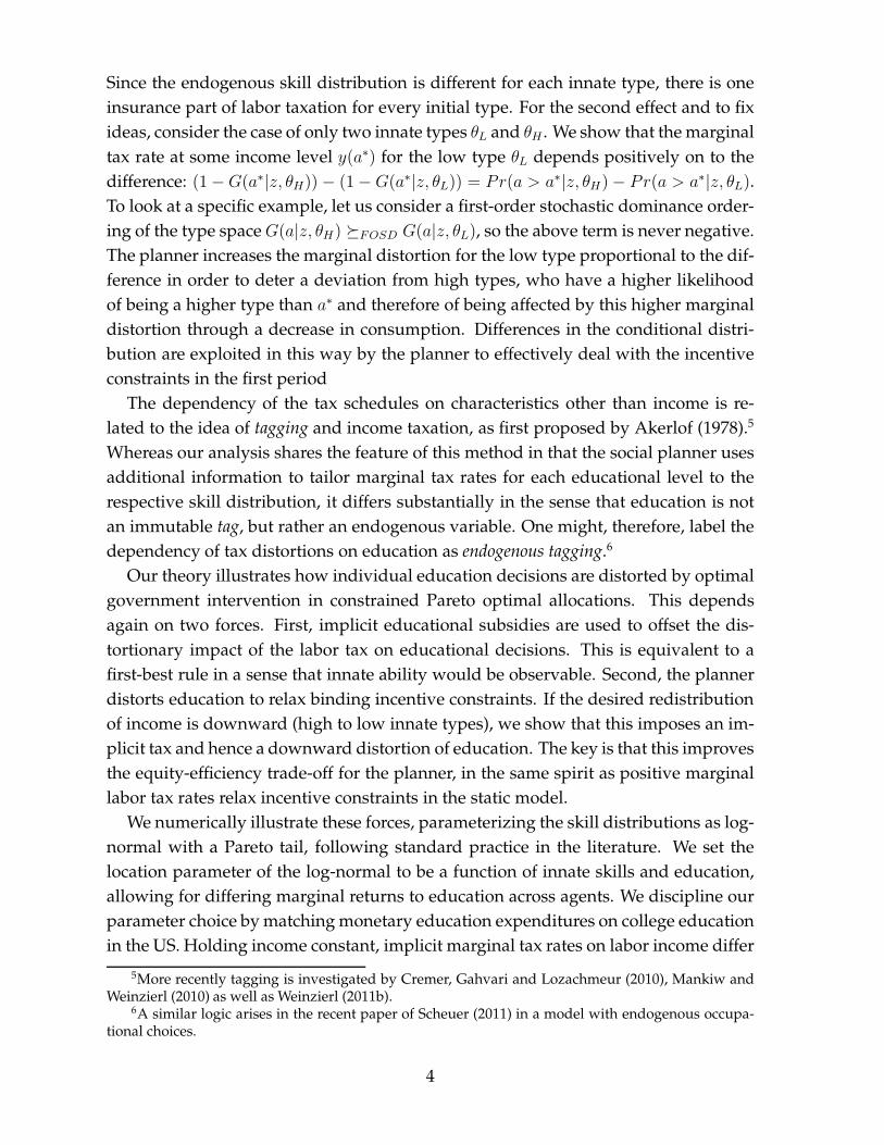
Figure 1 plots four exemplary density functions for two levels of θ and z, highlight-ing how a higher initial type and a higher education level translate into a right shiftof the distribution and a smaller peak.

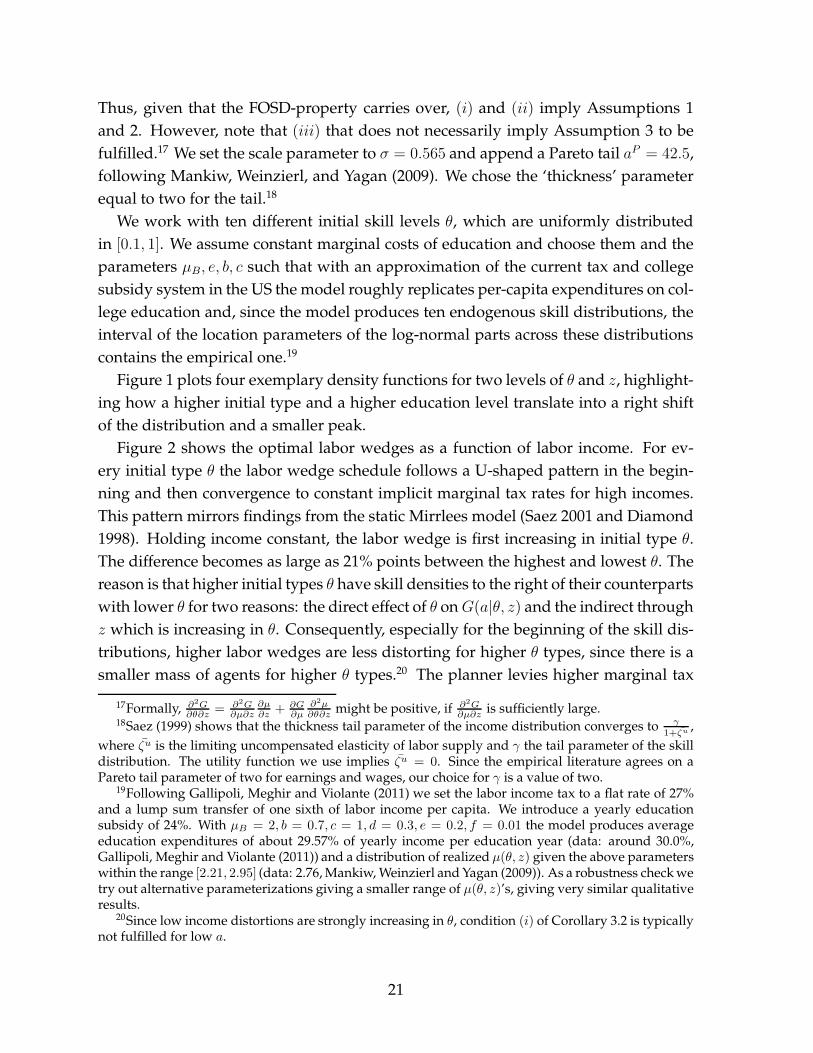
Figure 2 shows the optimal labor wedges as a function of labor income. For ev-ery initial type θ the labor wedge schedule follows a U-shaped pattern in the begin-ning and then convergence to constant implicit marginal tax rates for high incomes.This pattern mirrors findings from the static Mirrlees model (Saez 2001 and Diamond1998). Holding income constant, the labor wedge is first increasing in initial type θ.The difference becomes as large as 21% points between the highest and lowest θ. Thereason is that higher initial types θ have skill densities to the right of their counterpartswith lower θ for two reasons: the direct effect of θ onG(a|θ, z) and the indirect throughz which is increasing in θ. Consequently, especially for the beginning of the skill dis-tributions, higher labor wedges are less distorting for higher θ types, since there is asmaller mass of agents for higher θ types.20 The planner levies higher marginal tax

17Formally, ∂2G∂θ∂z

= ∂2G∂µ∂z

∂µ∂z

+ ∂G∂µ

∂2µ∂θ∂z

might be positive, if ∂2G∂µ∂z

is sufficiently large.18Saez (1999) shows that the thickness tail parameter of the income distribution converges to γ

1+ζu,

where ζu is the limiting uncompensated elasticity of labor supply and γ the tail parameter of the skilldistribution. The utility function we use implies ζu = 0. Since the empirical literature agrees on aPareto tail parameter of two for earnings and wages, our choice for γ is a value of two.

19Following Gallipoli, Meghir and Violante (2011) we set the labor income tax to a flat rate of 27%and a lump sum transfer of one sixth of labor income per capita. We introduce a yearly educationsubsidy of 24%. With µB = 2, b = 0.7, c = 1, d = 0.3, e = 0.2, f = 0.01 the model produces averageeducation expenditures of about 29.57% of yearly income per education year (data: around 30.0%,Gallipoli, Meghir and Violante (2011)) and a distribution of realized µ(θ, z) given the above parameterswithin the range [2.21, 2.95] (data: 2.76, Mankiw, Weinzierl and Yagan (2009)). As a robustness check wetry out alternative parameterizations giving a smaller range of µ(θ, z)’s, giving very similar qualitativeresults.

20Since low income distortions are strongly increasing in θ, condition (i) of Corollary 3.2 is typicallynot fulfilled for low a.

21

0 10 20 30 40 50 60 70 80 90 1000

0.005

0.01

0.015

0.02

0.025

0.03

0.035

0.04

0.045Skill Distributions

Den

sity

g(a

|...)

Ability Level

Theta=0.20, z=0.42Theta=0.20, z=2.95Theta=0.79, z=0.42Theta=0.79, z=2.95

Figure 1: Skill Distributions

rates on higher θ types, raising tax revenues with less distortions. Since the ‘hump’ ofthe densities of a is shifted to the right for higher θ, labor wedges decrease in θ in re-gions where the mass is increasing in θ. For large incomes all labor wedges convergeto a similar top rate because all distributions are characterized by a Pareto tail. Thedifferences in the tails can become as big as 4% points, however.

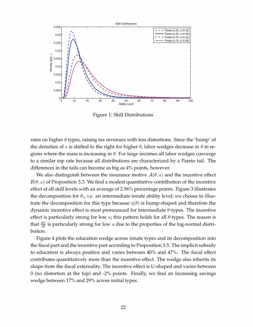
We also distinguish between the insurance motive A(θ, a) and the incentive effectB(θ, a) of Proposition 3.3. We find a modest quantitative contribution of the incentiveeffect at all skill levels with an average of 2.56% percentage points. Figure 3 illustratesthe decomposition for θ5, i.e. an intermediate innate ability level; we choose to illus-trate the decomposition for this type because η(θ) is hump-shaped and therefore thedynamic incentive effect is most pronounced for intermediate θ-types. The incentiveeffect is particularly strong for low a; this pattern holds for all θ-types. The reason isthat ∂G

∂θis particularly strong for low a due to the properties of the log-normal distri-

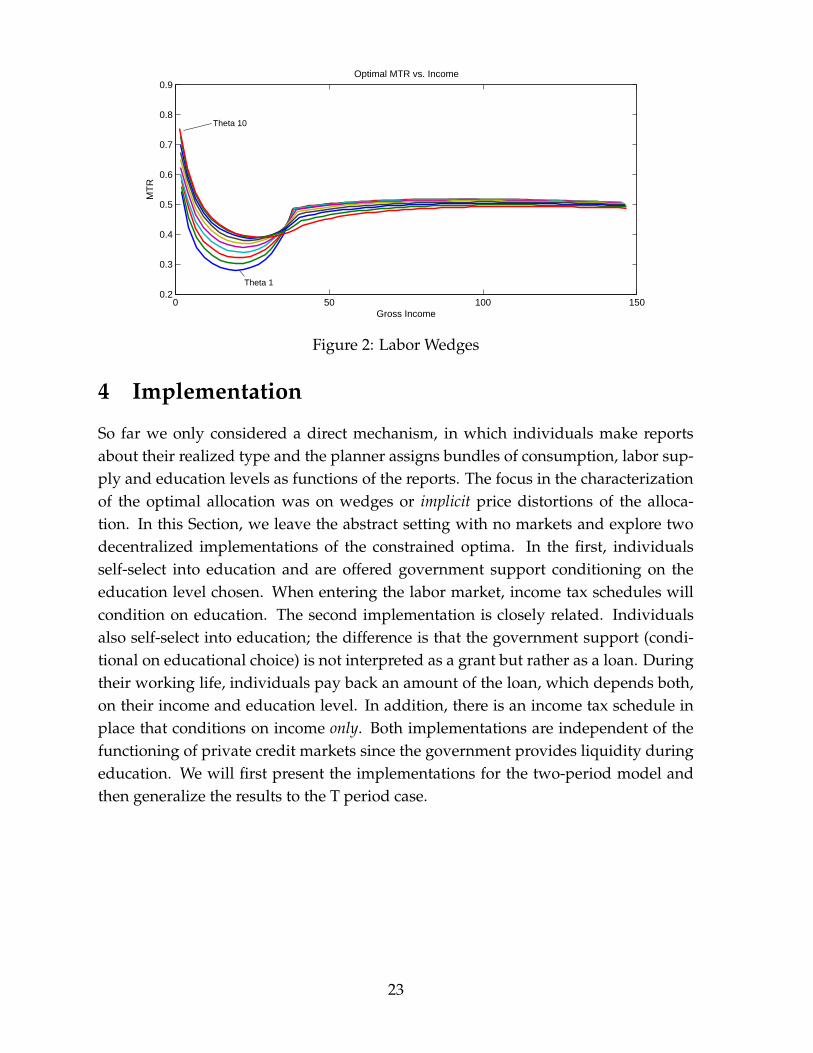
bution.Figure 4 plots the education wedge across innate types and its decomposition into

the fiscal part and the incentive part according to Proposition 3.5. The implicit subsidyto education is always positive and varies between 40% and 47%. The fiscal effectcontributes quantitatively more than the incentive effect. The wedge also inherits itsshape from the fiscal externality. The incentive effect is U-shaped and varies between0 (no distortion at the top) and -2% points. Finally, we find an increasing savingswedge between 17% and 29% across initial types.

22

0 50 100 1500.2

0.3

0.4

0.5

0.6

0.7

0.8

0.9Optimal MTR vs. Income

MT

R

Gross Income

Theta 10

Theta 1

Figure 2: Labor Wedges

4 Implementation

So far we only considered a direct mechanism, in which individuals make reportsabout their realized type and the planner assigns bundles of consumption, labor sup-ply and education levels as functions of the reports. The focus in the characterizationof the optimal allocation was on wedges or implicit price distortions of the alloca-tion. In this Section, we leave the abstract setting with no markets and explore twodecentralized implementations of the constrained optima. In the first, individualsself-select into education and are offered government support conditioning on theeducation level chosen. When entering the labor market, income tax schedules willcondition on education. The second implementation is closely related. Individualsalso self-select into education; the difference is that the government support (condi-tional on educational choice) is not interpreted as a grant but rather as a loan. Duringtheir working life, individuals pay back an amount of the loan, which depends both,on their income and education level. In addition, there is an income tax schedule inplace that conditions on income only. Both implementations are independent of thefunctioning of private credit markets since the government provides liquidity duringeducation. We will first present the implementations for the two-period model andthen generalize the results to the T period case.

23

0 50 100 1500

0.1

0.2

0.3

0.4

0.5

0.6

0.7Decomposition of the Labor Wedge

Gross Income

Labor WedgeInsurance PartDynamic Incentive Part

Figure 3: Decomposition of the Labor wedge

1 2 3 4 5 6 7 8 9 100.4

0.41

0.42

0.43

0.44

0.45

0.46

0.47

0.48

0.49

0.5Educational Wedge and Fiscal Externality

Edu

catio

nal W

edge

/Fis

cal E

xter

nalit

y

Innate Ability Level

Educational WedgeFiscal Externality

(a) Fiscal Externality

1 2 3 4 5 6 7 8 9 10−0.02

−0.018

−0.016

−0.014

−0.012

−0.01

−0.008

−0.006

−0.004

−0.002

0

(b) Incentive Effect

Figure 4: Educational Wedge

4.1 Implementation 1: Student Grants and Income Taxes Condition-

ing on Education

4.1.1 Two Periods

The benevolent government, taking the role of the planner, offers a menu of studentgrants to the agents. These grants G are conditional on education. In the secondperiod, there is a tax schedule in place, which, importantly, does not only condition onearnings but also on educational investment. Further, savings taxes are high enoughto make private savings disappear from the market; the definition of the savings taxbuilds on Werning (2011). We summarize this in the following proposition:

24

Proposition 4.1. Any constrained Pareto optimal allocation in a two period economy can

be implemented by a Grant schedule G(z), an education dependent income tax T (y, z) and a

savings tax T s(s), where

• G(z(θ)) = z(θ) + c1(θ)

• T (y(θ, a), z(θ)) = y(θ, a)− c2(θ, a)

• T s(s) as defined in Appendix A.5.

Proof. See Appendix A.5

Implementation of the savings wedges: The savings function T s(s) is prohibitivelyhigh such that all agents choose s = 0, hence in this implementation there are no pri-vate savings. However, as shown in Werning (2011) this comes without loss of gener-ality: by a Ricardian equivalence argument, we can adjust G(z(θ)) and T (y(θ, a), z(θ))with lump-sum transfers and deductibles to arrive with a non-linear savings tax sched-ule, which produces non-zero private savings for every agent and the same allocationwith the same distortion of consumption across periods. The full argument is foundin Werning (2011).

Implementation of the labor wedges: Agents enter the second period with nosavings as argued above. Their budget constraint is then: T (y(θ, a), z(θ)) = y(θ, a) −

c2(θ, a). From the agents’ optimality conditions for y and c2 it follows that marginaltax rates Ty(y(θ, a), z(θ)) are equal to labor wedges τy(θ, a) as characterized in Sec-tion 3.2.2.

Implementation of the education wedges: To fix ideas, the budget constraints ofan agent in both periods are given by:

c1(θ) + z(θ) ≤ G(z(θ))

c2(θ, a) ≤ y(θ, a)− T (z(θ), y(θ, a)),

where we already imposed the zero savings. In contrast to the optimal labor wedge,which equals the optimal labor tax, there is no single policy instrument for which theeducation wedge equals the marginal distortion of the policy. Instead, the govern-ment uses two instruments: i) the non-linear grant schedule G(z), which depends oneducation chosen and ii) the labor tax code in the second period. Using the agents’optimality conditions in the proposed implementation one can show that the wedgeequals:

τz(θ) = G ′(z)−

∫ a

a

u′(c2(θ, a))

u′(c1(θ))g(a|z(θ), θ)Tz(y(θ, a), z(θ))da

25

A positive value of τz(θ) encourages education at level θ. The incentive for agentsto increase their educational attainment comes from: i) An increase in their grantmeasured by G ′(z)21 and ii) an increase or decrease in their labor income tax burdenfor all states, i.e. Tz(y(θ, a), z(θ)).

4.1.2 T Periods

The possible extension to the life-cycle case is summarized as follows:

Corollary 4.2. Any constrained Pareto optimal allocation in a T-period economy can be im-

plemented by a Grant schedule G(z), an education dependent income tax Tt(yt, z) that condi-

tions on the history of incomes and a savings tax T s(s).

Proof. See Appendix A.6

The corollary is an application of insights from Werning (2007), who characterizespossible implementations in the dynamic deterministic Mirrlees problem. The prob-lem here is similar to his model with the only difference that there is not only one taxschedule conditioning on the history of incomes yt, but rather one for each θ-type oreach education level z.

One might wonder why the optimum is not simply implementable with time in-dependent schedules. The reason is that with such a tax system it might be possiblefor an individual to profit from tax arbitrage, if tax schedules are sufficiently concave.Instead of earning the assigned income y every period, it can then be favorable for anindividual to earn y − ǫ today and y + ǫ tomorrow. Average gross income would bethe same, however, due to concavity of T (y) the tax burden would decrease; if this ef-fect is strong enough, it might compensate for the higher disutility of labor. In realitysuch strategic behavior to exploit the non-linearity of the tax system seems unlikelyto occur. The reason is that shifting labor income between periods in such a way isoften very costly or simply infeasible due to adjustment costs and hours restrictions.22

Formally, let C(y∗) denote the present value of total adjustment costs of an individualthat chooses income history y∗, and if y∗Te+1 = y∗Te+2 = ... = y∗T , then C(y∗) = 0, so iflabor supply is constant, there are no adjustment costs.

Definition For a given adjustment cost function C(·), an income tax schedule T (y, z)is tax arbitrage resistant, if V (y∗, c∗(y∗, T (y, z(θ)), C(y∗)) ≤ V (ytruth(θ, a), ctruth(θ, a)) ∀ y∗

and ∀ (θ, a), where c∗(y∗, T (y), C(y∗)) is the optimal consumption sequence given y∗,

21Theoretically it could be the case that G is (partly) decreasing in z if c1(θ) is sufficiently decreasing.However, this is rather unlikely and in all our numerical examples we have c′1(θ) > 0.

22For a recent treatment of hours constraint in the public economics literature see Chetty, Friedman,Olsen and Pistaferri (2011); for the implications of adjustment costs on hours choices and the laborsupply elasticity see Chetty (2011).

26

T (y) and V (·, ·) is the respective (deterministic) working life utility conditional on therealization of a.

With this in mind, we make the following assumption stating that strategic deviationsare never feasible for a worker because of adjustment costs:

Assumption 4: The adjustment cost function C(·) is such that the income tax sched-ules T (y, z) with T (y(θ, a), z(θ)) = y(θ, a)− cw(θ, a) are tax arbitrage resistant.

This allows to implement constrained efficient allocation using a labor tax systemthat conditions on current income and one’s education level only, summarized in thefollowing corollary:

Corollary 4.3. Assume that Assumption 4 holds. Then any constrained Pareto optimal al-

location in a T-period economy can be implemented by a grant schedule G(z), an education

dependent income tax T (y, z) with T (y(θ, a), z(θ)) = y(θ, a) − cw(θ, a) and a savings tax

T s(s).

Proof. By Assumption 4 we know that individuals prefer yT (θ, a) over any incomesequence where y is not constant over time. By incentive compatibility we know thateach individual prefers yT (θ, a) over yT (θ, a′) ∀ a′, a; combining this with the insightsof Proposition 4.1 yields the result.

4.2 Implementation Two: Student Loans with Income-Contingent

Repayment

4.2.1 Two Periods

The previous implementation required that people with the same income but differ-ent levels of education pay different taxes. In reality people might perceive this asa violation of horizontal equity concerns, which could hinder the political feasibilityof such policies. In this light we now present a more appealing alternative imple-mentation with only one labor income tax schedule and a repayment scheme of theeducation grant.23 Technically, this can be seen as a simple reinterpretation of the pre-vious implementation – we take the tax system of the θ as the common labor incometax schedule and introduce an income-contingent repayment schedule, which condi-tions on the size of the loan.24 Together both instruments are sufficient to replicate theoptimal labor wedges. Formally we summarize this in the following proposition:

23Diamond and Saez (2011) argue in a recent contribution that practical policy prescription fromoptimal tax models should not go against common hold normative views (horizontal equity for exam-ple) and limit complexity to a reasonable degree. The second implementation seems in line with theserecommendations.

24Related implementations are of course possible where the tax function of another θ-type can bethe labor income tax schedule in place. In fact, somehow anything goes. The extreme case would just

27

Proposition 4.4. A constrained Pareto optimal allocation in a two-period economy can be

implemented by a Loan schedule L(z), a Loan Repayment Schedule Γ(y, L), an income tax

T (y) and a savings tax T s(s), where

• L(z(θ)) = z(θ) + c1(θ)

• Γ(y(θ, a), L(z(θ))) = c2(θ, a(θ, y(θ, a))) − c2(θ, a) if y ∈ [y(θ, a), y(θ, a)] and

Γ(y(θ, a), L(z(θ))) = y(θ, a)− c2(θ, a) otherwise.

• T (y) = y − c2(θ, a(θ, y)) ∀ y ∈ [y(θ, a), y(θ, a)] and T = 0 otherwise.

• T s(s) as defined in Appendix A.5.

where a(θ, y) is the inverse of y(θ, ·) for a.

Proof. The budget constraint of an individual reads as:

c1(θ) + z(θ) ≤ L(z(θ))

c2(θ, a) ≤ y(θ, a)− T (y(θ, a))− Γ(y(θ, a), L(z(θ))),

which is equivalent to the budget constraint in Implementation 1 since by definitionG(z) = L(z) ∀ z and T (y, z) = T (y) + Γ(y, z) ∀ y, z. Hence it is a direct consequence ofProposition 4.1.

4.2.2 T Periods

We will now show to what extend these results carry over to the case of T -periods.

Corollary 4.5. Any constrained Pareto optimal allocation in a T-period economy can be im-

plemented by a Loan schedule L(z), a Loan Repayment Schedule Γt(yt, L), an income tax

Tt(yt) and a savings tax T s(s).

In the same way as Corollary 4.2 follows from Proposition 4.1, this Corollary fol-lows from Proposition 4.4, we therefore omit a formal proof. Now we show that usingAssumption 4 the dependence of these policy instruments on the histories of incomescan be overcome.

Corollary 4.6. Assume that Assumption 4 holds. Then any constrained Pareto optimal allo-

cation in a T-period economy can be implemented by a Loan schedule L(z), a Loan Repayment

Schedule Γ(y, L), that is constant over time, an income tax T (y) that is constant over time

and a savings tax T s(s).

be to say that income taxes do not exist and all schedules that were interpreted as history dependentlabor income schedules in implementation 1 can now be interpreted as repayment schedules. Takingthe labor income tax schedule of the θ-type, however, seems to be more natural in our view. Especiallyin our application of the theory in Section 5.

28

Again we omit a formal proof as the result follows from Corollary 4.5 in the sameway as Corollary 4.3 follows from Corollary 4.2. The implementation is appealing,since is there is only one labor tax schedule and a yearly income contingent repaymentplan for each loan size.

5 An Application of the Model: College vs. High-School

We now present an empirically driven application of our model. We limit educationto be a binary instead of a continuous choice. Agents either enter the labor marketdirectly after high-school graduation or go to college before working. Additionally,we restrict the analysis to two different levels of innate ability.25 These simplifica-tions enable us to parameterize the model using factual and, importantly, estimatedcounterfactual earnings distributions from the empirical labor literature (Cunha andHeckman 2007, 2008). Further the simplification has the advantage that it is easy to in-corporate foregone earnings as an implicit cot of education. As laid out in Proposition3.4, these counterfactual terms contribute to optimal marginal tax rates by deterringdeviations. The simplified model, arguably, also comes a step closer to more practicalpolicy recommendations, since the optimum can be implemented with considerablyless complexity; one non-linear labor income tax schedule and one non-linear repay-ment schedule for college loans will suffice in the application.

5.1 Parametrization

Agents live for 49 years after they graduate from high-school (age 16-65). Afterwardsthey enter the labor market directly, or decide to go to college and graduate in fouryears. We label the two innate types θHS and θCO and assume that it is a priori optimalthat θHS chooses the lower educational attainment (high school) and that θCO choosesthe higher educational attainment (college). We solve for the utilitarian optimum. The(binding) incentive constraint for type θCO, hence, reads as:

3∑

t=0

βtu(c1(θCO)) +

48∑

t=4

βt

∫ a

a

v2(a, θCO)g(a|CO, θCO)da

=

48∑

t=0

βt

∫ a

a

v2(a, θHS)g(a|HS, θCO), (8)

25This strong assumption implies that all individuals with the same education level are ex-anteequal, which is clearly not realistic. It can be seen as an indispensable approximation, which we needto make in order to identify innate types from real world data.

29

0 2 4 6 8 10 12 14 16 18

x 104

0

0.005

0.01

0.015

0.02

0.025

0.03

0.035

0.04

Gross Income

High SchoolCollege FactualCollege Counterfactual

Figure 5: Earnings Distributions

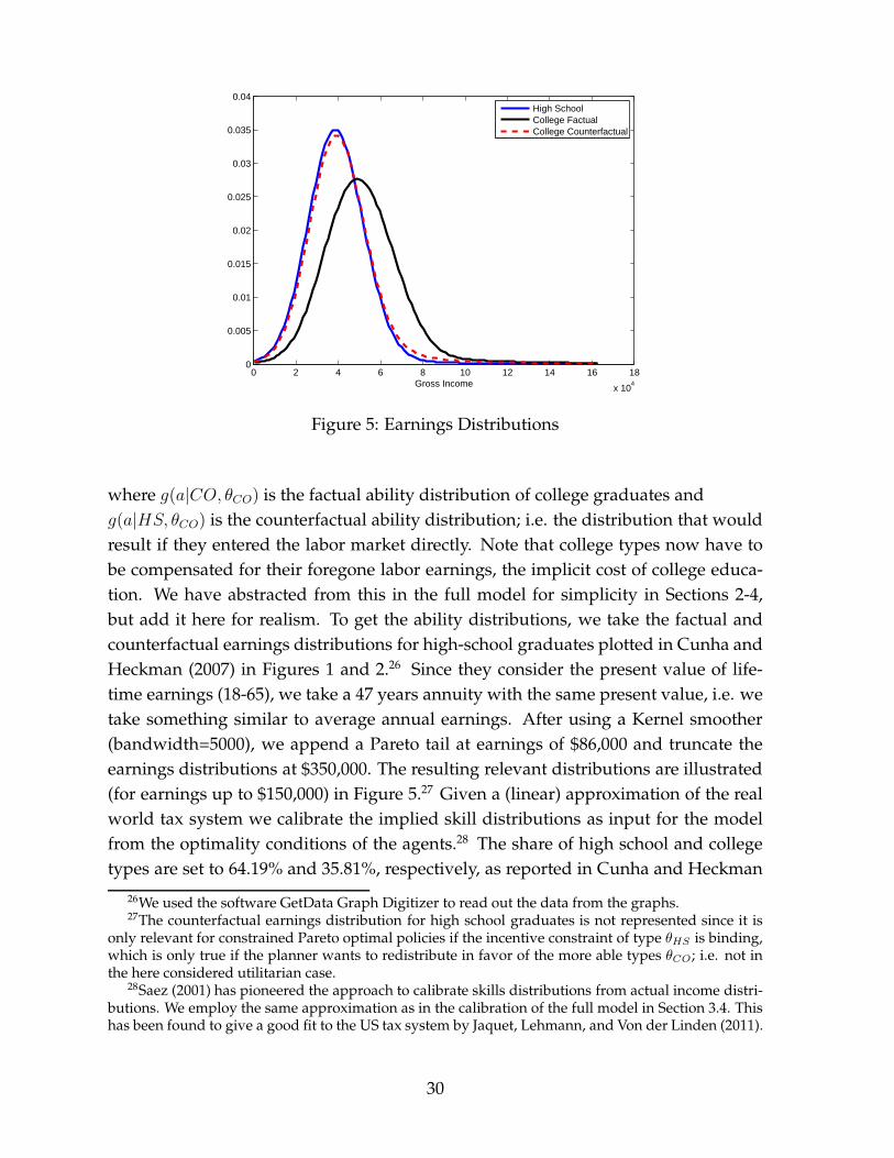
where g(a|CO, θCO) is the factual ability distribution of college graduates andg(a|HS, θCO) is the counterfactual ability distribution; i.e. the distribution that wouldresult if they entered the labor market directly. Note that college types now have tobe compensated for their foregone labor earnings, the implicit cost of college educa-tion. We have abstracted from this in the full model for simplicity in Sections 2-4,but add it here for realism. To get the ability distributions, we take the factual andcounterfactual earnings distributions for high-school graduates plotted in Cunha andHeckman (2007) in Figures 1 and 2.26 Since they consider the present value of life-time earnings (18-65), we take a 47 years annuity with the same present value, i.e. wetake something similar to average annual earnings. After using a Kernel smoother(bandwidth=5000), we append a Pareto tail at earnings of $86,000 and truncate theearnings distributions at $350,000. The resulting relevant distributions are illustrated(for earnings up to $150,000) in Figure 5.27 Given a (linear) approximation of the realworld tax system we calibrate the implied skill distributions as input for the modelfrom the optimality conditions of the agents.28 The share of high school and collegetypes are set to 64.19% and 35.81%, respectively, as reported in Cunha and Heckman

26We used the software GetData Graph Digitizer to read out the data from the graphs.27The counterfactual earnings distribution for high school graduates is not represented since it is

only relevant for constrained Pareto optimal policies if the incentive constraint of type θHS is binding,which is only true if the planner wants to redistribute in favor of the more able types θCO; i.e. not inthe here considered utilitarian case.

28Saez (2001) has pioneered the approach to calibrate skills distributions from actual income distri-butions. We employ the same approximation as in the calibration of the full model in Section 3.4. Thishas been found to give a good fit to the US tax system by Jaquet, Lehmann, and Von der Linden (2011).

30

0 5 10 15

x 104

0.1

0.2

0.3

0.4

0.5

0.6

0.7

0.8

0.9Optimal MTR vs. Income

MT

R

Gross Income

High SchoolCollege

Figure 6: Optimal Marginal Tax Rates

(2008). Following Gallipoli, Meghir and Violante (2011) we set the annual monetarycost of college education to $7,900.29 The flow utility function, the yearly discountfactor and the interest rate take the same values as in Section 3.4.

5.2 Results

5.2.1 Two Income Tax Schedules

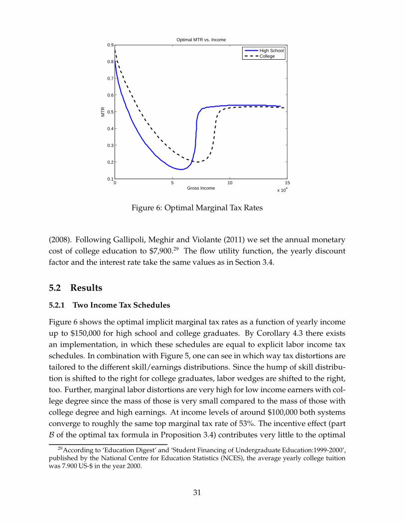
Figure 6 shows the optimal implicit marginal tax rates as a function of yearly incomeup to $150,000 for high school and college graduates. By Corollary 4.3 there existsan implementation, in which these schedules are equal to explicit labor income taxschedules. In combination with Figure 5, one can see in which way tax distortions aretailored to the different skill/earnings distributions. Since the hump of skill distribu-tion is shifted to the right for college graduates, labor wedges are shifted to the right,too. Further, marginal labor distortions are very high for low income earners with col-lege degree since the mass of those is very small compared to the mass of those withcollege degree and high earnings. At income levels of around $100,000 both systemsconverge to roughly the same top marginal tax rate of 53%. The incentive effect (partB of the optimal tax formula in Proposition 3.4) contributes very little to the optimal

29According to ‘Education Digest’ and ‘Student Financing of Undergraduate Education:1999-2000’,published by the National Centre for Education Statistics (NCES), the average yearly college tuitionwas 7.900 US-$ in the year 2000.

31

0 5 10 15

x 104

3000

4000

5000

6000

7000

8000

9000

10000

11000Yearly Repayment vs. Income

Rep

aym

ent

Gross Income

Figure 7: Yearly Repayment

high school tax schedule. Ignoring it would yield optimal tax rates, which differ by0.17% percentage points on average (weighted by income and density). This is consis-tent with Figure 5 showing that college types only have a slight distributional advan-tage over high school types, conditional on entering the labor market directly afterhigh school. So, although the model requires counterfactual distribution to includethe influence of dynamic incentive effects deterring deviations, these effects seem tohave a negligible impact on optimal marginal tax rates. This suggests that even with-out estimates of distributions for counterfactual education choices, meaningful taxsimulations can be conducted.

5.2.2 One Income Tax Schedule and Repayments for College Graduates

By Corollary 4.6 one can interpret the marginal tax rates of the θHS-type(s) in Fig-ure 6 as marginal tax rates of an income tax schedule common to all individuals. Themarginal tax rates for the θCO-type in Figure 6 can, instead, also be interpreted as theaggregate of marginal distortion through the income tax and an income-dependentloan repayment schedule. The loan repayment schedule yielding the correct aggre-gate marginal distortions is illustrated in Figure 7. Repayment first increases withincome and then drastically decreases before it converges.30 One might wonder whythe schedule is not increasing in y as an insurance device against labor market risk.The reason is that the labor income tax schedule also acts as an insurance device andactually their interaction yields optimal insurance. The common income tax schedule

30It still decreases slightly in the graph, however, this is due to the truncation of the distributionmade in our simulation. If the distributions were unbounded, the loan repayment would converge aslong as the term B(Y ) in the labor wedge formula is negligible, which is the case in our simulations.

32

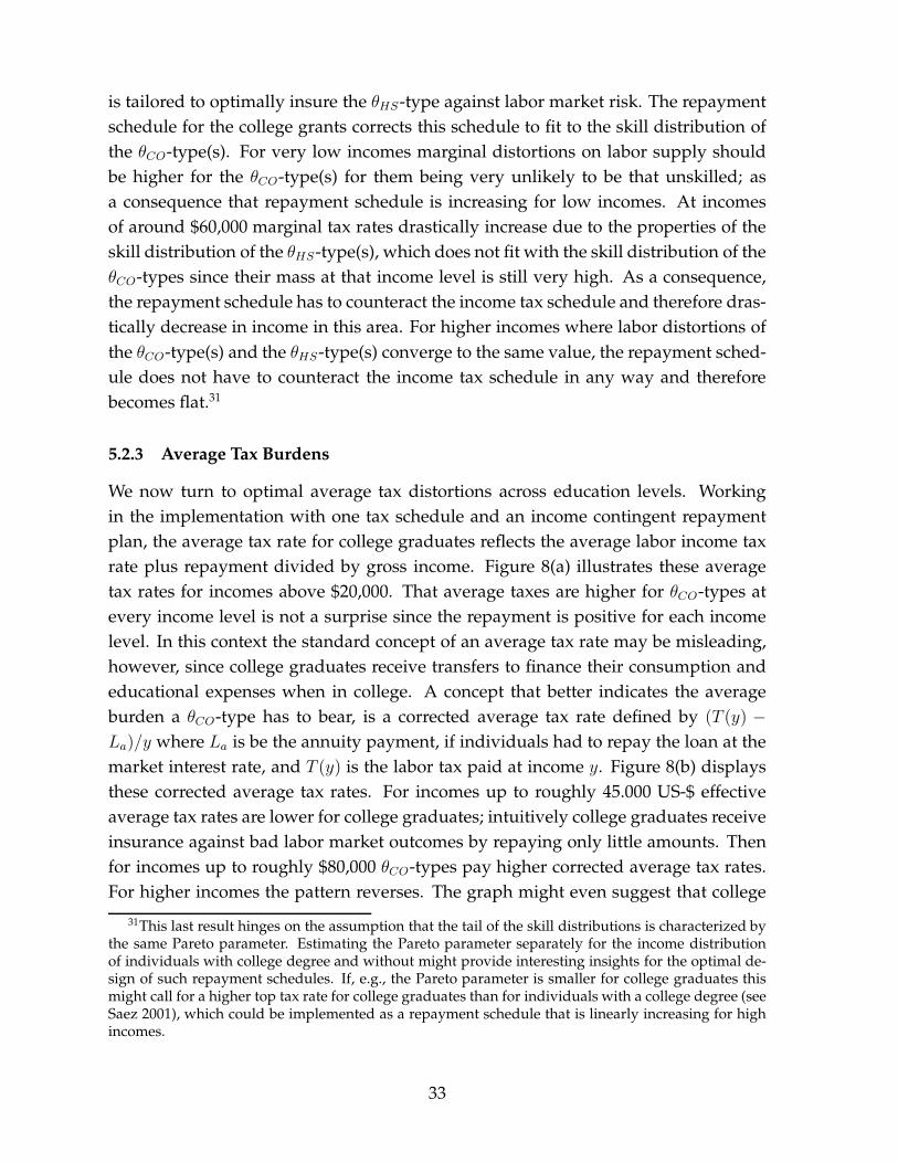
is tailored to optimally insure the θHS-type against labor market risk. The repaymentschedule for the college grants corrects this schedule to fit to the skill distribution ofthe θCO-type(s). For very low incomes marginal distortions on labor supply shouldbe higher for the θCO-type(s) for them being very unlikely to be that unskilled; asa consequence that repayment schedule is increasing for low incomes. At incomesof around $60,000 marginal tax rates drastically increase due to the properties of theskill distribution of the θHS-type(s), which does not fit with the skill distribution of theθCO-types since their mass at that income level is still very high. As a consequence,the repayment schedule has to counteract the income tax schedule and therefore dras-tically decrease in income in this area. For higher incomes where labor distortions ofthe θCO-type(s) and the θHS-type(s) converge to the same value, the repayment sched-ule does not have to counteract the income tax schedule in any way and thereforebecomes flat.31

5.2.3 Average Tax Burdens

We now turn to optimal average tax distortions across education levels. Workingin the implementation with one tax schedule and an income contingent repaymentplan, the average tax rate for college graduates reflects the average labor income taxrate plus repayment divided by gross income. Figure 8(a) illustrates these averagetax rates for incomes above $20,000. That average taxes are higher for θCO-types atevery income level is not a surprise since the repayment is positive for each incomelevel. In this context the standard concept of an average tax rate may be misleading,however, since college graduates receive transfers to finance their consumption andeducational expenses when in college. A concept that better indicates the averageburden a θCO-type has to bear, is a corrected average tax rate defined by (T (y) −

La)/y where La is be the annuity payment, if individuals had to repay the loan at themarket interest rate, and T (y) is the labor tax paid at income y. Figure 8(b) displaysthese corrected average tax rates. For incomes up to roughly 45.000 US-$ effectiveaverage tax rates are lower for college graduates; intuitively college graduates receiveinsurance against bad labor market outcomes by repaying only little amounts. Thenfor incomes up to roughly $80,000 θCO-types pay higher corrected average tax rates.For higher incomes the pattern reverses. The graph might even suggest that college

31This last result hinges on the assumption that the tail of the skill distributions is characterized bythe same Pareto parameter. Estimating the Pareto parameter separately for the income distributionof individuals with college degree and without might provide interesting insights for the optimal de-sign of such repayment schedules. If, e.g., the Pareto parameter is smaller for college graduates thismight call for a higher top tax rate for college graduates than for individuals with a college degree (seeSaez 2001), which could be implemented as a repayment schedule that is linearly increasing for highincomes.

33

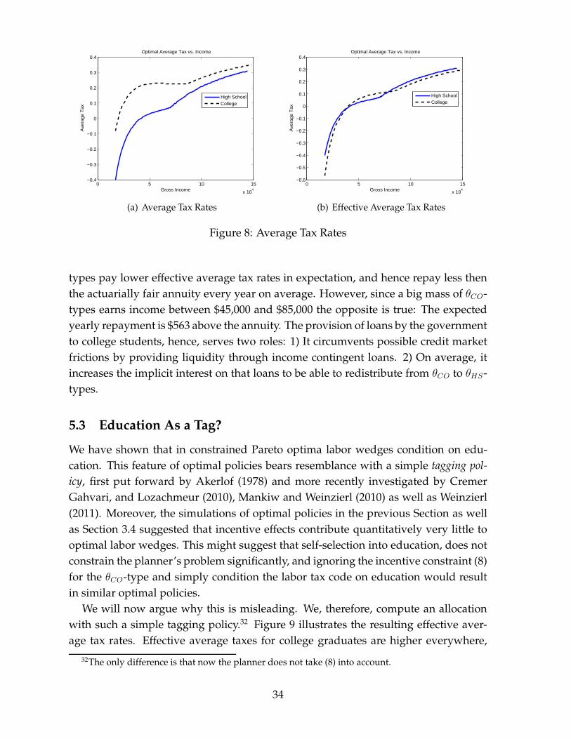
0 5 10 15

x 104

−0.4

−0.3

−0.2

−0.1

0

0.1

0.2

0.3

0.4Optimal Average Tax vs. Income

Ave

rage

Tax

Gross Income

High SchoolCollege

(a) Average Tax Rates

0 5 10 15

x 104

−0.6

−0.5

−0.4

−0.3

−0.2

−0.1

0

0.1

0.2

0.3

0.4Optimal Average Tax vs. Income

Ave

rage

Tax

Gross Income

High SchoolCollege

(b) Effective Average Tax Rates

Figure 8: Average Tax Rates

types pay lower effective average tax rates in expectation, and hence repay less thenthe actuarially fair annuity every year on average. However, since a big mass of θCO-types earns income between $45,000 and $85,000 the opposite is true: The expectedyearly repayment is $563 above the annuity. The provision of loans by the governmentto college students, hence, serves two roles: 1) It circumvents possible credit marketfrictions by providing liquidity through income contingent loans. 2) On average, itincreases the implicit interest on that loans to be able to redistribute from θCO to θHS-types.

5.3 Education As a Tag?

We have shown that in constrained Pareto optima labor wedges condition on edu-cation. This feature of optimal policies bears resemblance with a simple tagging pol-

icy, first put forward by Akerlof (1978) and more recently investigated by CremerGahvari, and Lozachmeur (2010), Mankiw and Weinzierl (2010) as well as Weinzierl(2011). Moreover, the simulations of optimal policies in the previous Section as wellas Section 3.4 suggested that incentive effects contribute quantitatively very little tooptimal labor wedges. This might suggest that self-selection into education, does notconstrain the planner’s problem significantly, and ignoring the incentive constraint (8)for the θCO-type and simply condition the labor tax code on education would resultin similar optimal policies.

We will now argue why this is misleading. We, therefore, compute an allocationwith such a simple tagging policy.32 Figure 9 illustrates the resulting effective aver-age tax rates. Effective average taxes for college graduates are higher everywhere,

32The only difference is that now the planner does not take (8) into account.

34

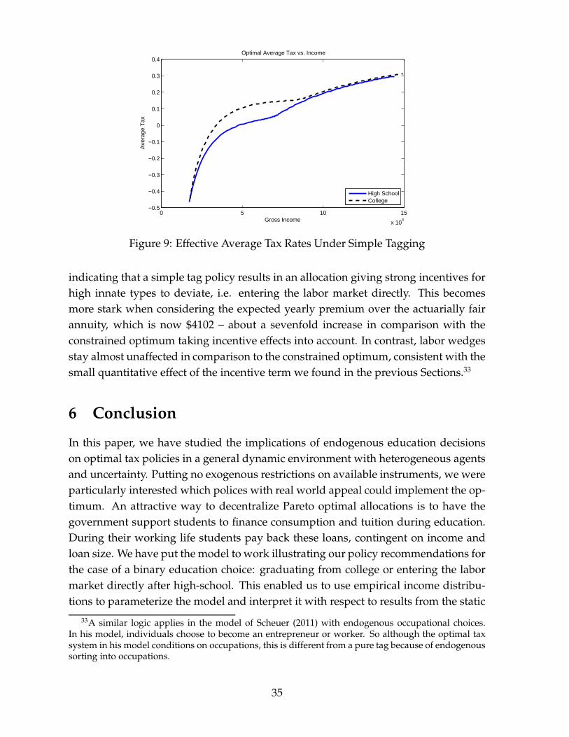
0 5 10 15

x 104

−0.5

−0.4

−0.3

−0.2

−0.1

0

0.1

0.2

0.3

0.4Optimal Average Tax vs. Income

Ave

rage

Tax

Gross Income

High SchoolCollege

Figure 9: Effective Average Tax Rates Under Simple Tagging

indicating that a simple tag policy results in an allocation giving strong incentives forhigh innate types to deviate, i.e. entering the labor market directly. This becomesmore stark when considering the expected yearly premium over the actuarially fairannuity, which is now $4102 – about a sevenfold increase in comparison with theconstrained optimum taking incentive effects into account. In contrast, labor wedgesstay almost unaffected in comparison to the constrained optimum, consistent with thesmall quantitative effect of the incentive term we found in the previous Sections.33

6 Conclusion

In this paper, we have studied the implications of endogenous education decisionson optimal tax policies in a general dynamic environment with heterogeneous agentsand uncertainty. Putting no exogenous restrictions on available instruments, we wereparticularly interested which polices with real world appeal could implement the op-timum. An attractive way to decentralize Pareto optimal allocations is to have thegovernment support students to finance consumption and tuition during education.During their working life students pay back these loans, contingent on income andloan size. We have put the model to work illustrating our policy recommendations forthe case of a binary education choice: graduating from college or entering the labormarket directly after high-school. This enabled us to use empirical income distribu-tions to parameterize the model and interpret it with respect to results from the static

33A similar logic applies in the model of Scheuer (2011) with endogenous occupational choices.In his model, individuals choose to become an entrepreneur or worker. So although the optimal taxsystem in his model conditions on occupations, this is different from a pure tag because of endogenoussorting into occupations.

35

literature (Saez 2001). The labor wedge of college graduates as a function of incomelies first strictly above their counterparts from high-school, but this reverses at higherincomes. The optimal repayment plan is hump-shaped and college graduates pay aslightly positive premium over the actuarially fair annuity in expectation.

We have abstracted from some several elements, which can be tackled in futurework. For example, the planner had full commitment to honor all utility promisesand deliver by history dependent distortions. Relaxing this assumption by incorpo-rating political economy aspects could yield interesting insights. There could be anadditional force to have a decreasing education subsidy; this keeps inequality in checkand thereby strengthens credibility, which in turn mitigates the detrimental effects ofthe lack of commitment on human capital investment. This would counteract the roleof increasing subsidies to offset the effect of progressive taxes, we found dominatingin our numerical section (Figure 4). This idea that current policies influence futurecredibility has recently been put forward by Farhi, Sleet, Werning, and Yeltekin (2011)for the case of capital taxation.

Finally, our simulation have shown that counterfactual distribution have a quanti-tatively small contribution to optimal marginal tax rates. So even without the avail-ability of counterfactual earnings distribution, meaningful tax simulation can be con-ducted for other countries than the US.

A Appendix

A.1 Properties of the Laissez-Faire Allocation

To show part (iv), we show that:

∂2U(s, z; θ, .)

∂s∂θ= −β

∫ a

a

∂2v2(a, s)

∂s∂a

∂G(a|z, θ)

∂θda (9)

= −β

∫ a

a

∂y(s, a)

∂s

[

Ψ′

(

y(s, a)

a

)

1

a2+Ψ′′

(

y(s, a)

a

)

y(s, a)

a2

]

∂G(a|z, θ)

∂θda < 0

∂2U(s, z; θ, .)

∂s∂z(10)

= u′′(c1(θ)− β

∫ a

a

∂y(s, a)

∂s

[

Ψ′

(

y(s, a)

a

)

1

a2+Ψ′′

(

y(s, a)

a

)

y(s, a)

a2

]

∂G(a|z, θ)

∂zda < 0

∂2U(s, z; θ, .)

∂z∂θ= −β

∫ a

a

∂v2(a, s)

∂a

∂2G(a|z, θ)

∂z∂θda > 0, (11)

applying the envelope theorem and integrating by parts several times, as well as allthree assumptions on the conditional distribution function. Also note that ∂y(s,a)

∂s< 0,

simply because of income effects.

36

A.2 Proof of Lemma 3.2

Consider some admissible reporting strategy r(θ) = θ′.

∂U(θ, θ′)

∂r(θ)= uc (c1 (θ

′))∂c1(θ

′)

∂r(θ)+ β

∫ a

a

∂v2(θ′, a)

∂r(θ)g(a|z(θ′), θ)da

+∂z(θ′)

∂r(θ)

∫ a

a

v2(θ′, a)

∂g(a|z(θ′), θ)

∂z(θ′)da

and

0 =∂U(θ′, θ′)

∂r(θ)= uc (c1 (θ

′))∂c1(θ

′)

∂r(θ)+ β

∫ a

a

∂v2(θ′, a)

∂r(θ)g(a|z(θ′), θ′)da

+∂z(θ′)

∂r(θ)

∫ a

a

v2(θ′, a)

∂g(a|z(θ′), θ′)

∂z(θ′)da

Subtracting from one another gives:

∂U(θ, θ′)

∂r(θ)= β

∫ a

a

[

∂v2(θ′, a)

∂r(θ)(g(a|z(θ′), θ)− g(a|z(θ′), θ′))

+∂z(θ′)

∂r(θ)v2(θ

′, a)

(

∂g(a|z(θ′), θ)

∂z(θ′)−∂g(a|z(θ′), θ′)

∂z(θ′)

)]

da.

We are now looking when this last expression always has the same sign as the dif-ference (θ − θ′), which is clearly sufficient for global incentive compatibility. For(θ − θ′) > 0, by Assumption 2, the first line is positive, if ∂v2(θ′,a)

∂r(θ)or equivalently

∂v2(θ,a)∂θ

in a truthful mechanism is increasing in a. This can be shown to be equivalentto ∂y(θ,a)

∂θ> 0 using the envelope theorem. The second line is positive if ∂z(θ′)

∂r(θ)> 0 or

equivalently ∂z(θ)∂θ

> 0 in a truthful mechanism. The last condition (iii) is a routineexercise and a proof can be found, for example in Salanié (2003).

37

A.3 Second Best Policies: Pareto Problem and Optimality Condi-

tions

maxc1(θ),v2(θ,a),z(θ),y(θ,a)

∫ θ

θ

u(c1(θ))dF (θ)

+ β

∫ θ

θ

∫ a

a

v2(θ, a)dG(a|z(θ), θ)dF (θ)

+1

RλR

∫ θ

θ

∫ a

a

y(θ, a)dG(a|z(θ), θ)dF (θ)

−1

RλR

∫ θ

θ

∫ a

a

u−1 [v2(θ, a) + Ψ (y(θ, a)/a)] dG(a|z(θ), θ)dF (θ)

− λR

∫ θ

θ

(c1(θ) + z(θ)) dF (θ)

−

∫ θ

θ

∫ a

a

(

µ′(θ, a)v2(θ, a) + µ(θ, a)Ψ′

(

y(θ, a)

a

)

y(θ, a)

a2

)

dadθ

−

∫ θ

θ

η′(θ)

[

u(c1(θ)) + β

∫ a

a

v2(θ, a)dG(a|z(θ))da

]

dθ

− β

∫ θ

θ

η(θ)

∫ a

a

v2(θ, a)∂g(a|z(θ), θ)

∂θdadθ

With first-order conditions:

u′(c1(θ))(f(θ)− η′(θ))− λRf(θ) = 0 (c1SB)

(

f(θ)− η′(θ))

βg(a|z(θ), θ)− λR1

R

1

u′(c2(θ, a))g(a|z(θ), θ)f(θ)− µ′(θ, a)

− β∂g(a|z (θ) , θ)

∂θη(θ) = 0 (v2SB)

1

RλRg(a|z(θ), θ)f(θ)− µ(θ, a)

[

Ψ′′

(

y(θ, a)

a

)

y(θ, a)

a3+

1

a2Ψ′

(

y(θ, a)

a

)]

−1

RλRg(a|z(θ), θ)f(θ)

Ψ′(

y(θ,a)a

)

au′(c2(θ, a))= 0, (ySB)

38

f(θ)β

∫ a

a

v2(θ, a)∂g(a|z(θ), θ)

∂z(θ)da+

1

RλRf(θ)

∫ a

a

∂g(a|z(θ), θ)

∂z(θ)(y(θ, a)− c2(θ, a)) da

−η′(θ)β

∫ a

a

v2(θ, a)∂g(a|z(θ), θ)

∂z(θ)da− βη(θ)

∫ a

a

v2(θ, a)∂2g(a|z(θ), θ)

∂z(θ)∂θda− λRf(θ) = 0

(zSB)

A.4 Proofs of Propositions 3.3-3.5

A.4.1 Proposition 3.3

Combining equations (c1SB) and (v2SB) and integrating directly gives the result.

A.4.2 Proposition 3.4

Rewriting (ySB):

λRg(a|z(θ), θ)f(θ)

1−Ψ′

(

y(θ,a)a

)

au′(c1(θ, a))

−Rµ(θ, a)

[

Ψ′′

(

y(θ, a)

a

)

y(θ, a)

a3+

1

a2Ψ′

(

y(θ, a)

a

)]

= 0.

Dividing by Ψ′

au′and λRg(a|z, θ)f(θ) and using the definition of the labor wedge, i.e.

u′(1− τy) = Ψ′ 1a

yields

τy(θ, a)

1− τ(θ, a)= R

µ(θ, a)

λRg(a|z(θ), θ)f(θ)a

[

Ψ′′ ya2

+Ψ′ 1a

Ψ′

au′

]

,

which can be written as

τy(θ, a)

1− τ(θ, a)= R ·

µ(θ, a)

λRg(a|z(θ), θ)f(θ)a

1 + εu(θ, a)

εc(θ, a),

where Ψ′ 1

a

Ψ′′ y

a2+Ψ′ 1

a

= 1+εu(θ,a)εc(θ,a)

can be shown by simple algebra, see Saez (2001, p.227).

In particular, with the isoelastic specification used in the computations (y/a)σ

σone can

verify that this term is equal to 1σ

.The multiplier µ(θ, a) can be obtained using (v2SB) and (c1SB):

µ(θ, a) =λRf(θ)

u′(c1(θ))βG(a|z(θ), θ)−

λRRf(θ)

∫ a

a

1

u′(c2(θ, a∗))dG(a∗|z(θ), θ)

−β∂G(a|z(θ), θ)

∂θη(θ∗),

39

yielding:τy(θ, a)

1− τ(θ, a)=

1 + εu(θ, a)

εc(θ, a)

u′(c2(θ, a))

ag(a|z(θ), θ)[A(θ, a) + B(θ, a)]

where

A(θ, a) =βRG(a|z(θ), θ)

u′(c1(θ))−

∫ a

a

1

u′(c2(θ, a∗))dG(a∗|z(θ), θ)

B(θ, a) = −1

f(θ)λRβR

∂G(a|z(θ), θ)

∂θη(θ).

Using the inverse Euler equation, the term A(θ, a) can be written as in Proposi-tion 3.3.

From (c1SB), η(θ) is given by:

η(θ) = F (θ)− λR

∫ θ

θ

1

u′(c1(θ))f(θ)dθ.

The direct benefit of raising utils for agents with skill lower than θ is F (θ). The mon-etary cost is

∫ θ

θ1

u′(c1(θ))f(θ)dθ, transformed into utils by λR.

Relation to the formula of Saez (2001)

The insurance part of the labor wedge can be expressed as in Saez (2001), for ourcase with separable preferences. This relation applies if agents do not differ ex-ante.By some abuse of notation, then B(θ, a) = 0 and for A(θ, a), using the inverse Eulerequation, we obtain

A(θ, a) =

∫ a

a

G(a|z(θ), θ)

u′(c2(θ, a∗))dG(a∗|z(θ), θ)−

∫ a

a

1

u′(c2(θ, a∗))dG(a∗|z(θ), θ)

=

∫ a

a

G(a|z(θ), θ)

u′(c2(θ, a∗))dG(a∗|z(θ), θ)−

∫ a

a

1

u′(c2(θ, a∗))dG(a∗|z(θ), θ)

+

∫ a

a

1

u′(c2(θ, a∗))dG(a∗|z(θ), θ)

=

∫ a

a

1

u′(c2(θ, a∗))dG(a∗|z(θ), θ)−

∫ a

a

1−G(a|z(θ), θ)

u′(c2(θ, a∗))dG(a∗|z(θ), θ)

where the second equality follows from the transversality condition. This term can beexpressed as in Saez (2001) as shown by Mankiw, Weinzierl and Yagan (2009) in theironline appendix.

40

A.4.3 Proposition 3.5

Plugging c1SB into zSB gives:

λRf(θ)

u′(c1(θ))β

∫ a

a

v2(θ, a)∂g(a|z(θ), θ)

∂z(θ)da+

1

RλRf(θ)

∫ a

a

∂g(a|z(θ), θ)

∂z(θ)(y(θ, a)− c2(θ, a)) da

− βη(θ)

∫ a

a

v2(θ, a)∂2g(a|z(θ), θ)

∂z(θ)∂θda− λRf(θ) = 0

Proposition 3.5 directly follows.

A.5 Proof of Proposition 4.1

Starting from a direct mechanism we show in four steps that optimal allocations canindeed be implemented with the policy instruments as defined in Proposition A.5.

Step 1: Introduce savings

Imagine the constrained efficient allocation is implemented by a direct mechanism.From that point on, assume that individuals could freely save s. With savings taxT s(s, r1), the budget constraints read as

c1(r1) + s = c1(r1) (12)

c2(r1, r2) = c2(r1, r2) +Rs− T s(s, r1) (13)

Define the optimal report r2 about a, for a given report r1 about θ, a given savingstax schedule T s(s, r1) and a given level of savings s:

r∗2(a, r1, s, T s) = argmax

r2u [c2(r1, r2) +Rs− T s(s, r1)]− ψ

(

y(r1, r2)

a

)

Then the optimal report in period 1, for a given level of savings and a given savingstax schedule T s(s, r1), is defined by

r∗1(θ, s, Ts(r1, s)) = argmax

r1u(c1(r1)− s)

+ β

∫ a

a

u [c2(r1, r∗2) +Rs− T s(s, r1)]− ψ

(

y(r1, r∗2)

a

)

dG(a|z(r1), θ) (14)

Then define a hypothetical tax schedule T ∗(r1, s, θ) for eaach θ implicitely by

V (θ) = V (θ, s, r∗1, T∗(r1, s, θ)) ∀ s.

41

This hypothetical tax schedule would make individuals of type θ indifferent betweentruth telling and the optimal joint deviation for any s. It is hypothetical since it doesnot only depend on the report r1, which is observable but also on the unobservabletype θ. However, we know that for each θ such a tax schedule exists. Therefore takingthe upper envelope over these functions, we define T (s, r1) by

T (s, r1) = supθT ∗(r1, s, θ) (15)

Lemma A.1. A constrained efficient allocation can be implemented by a direct mechanism

extended by a savings choice and history dependent savings tax schedules T s(s, r1).

Step 2: Make the savings tax history independent

A simple way to make the savings tax history-independent is to take the upperenvelope of all function T s(s, r1), i.e.

T s(s) = supr1

T s(s, r1). (16)

Lemma A.2. A constrained efficient allocation can be implemented by a direct mechanism

extended by a savings choice and history independent savings tax schedules T s(s).

Step 3: Allow for labor-leisure decisions

To get closer to a decentralized implementation now assume the following ex-tended direct mechanism.

1. Individuals report r(θ)

2. They get assigned ’income to consume’ c1(θ)

3. They face the savings tax schedule T s(s) and save s(θ) = 0

4. In period two, instead of directly revealing their type, individuals of type θ facean income tax schedule that is defined by

T (y(θ, a), θ) = y(θ, a)− c2(θ, a)) ∀ a

By the same arguments as in the standard Mirrlees model it follows that this ex-tended direct mechanism can also implement the constrained efficient allocations.

We can summarize this in the following lemma.

Lemma A.3. A constrained efficient allocation can be implemented by a direct mechanism in

the first period extended by a savings choice and a history independent differentiable savings

tax schedule T s(s) and a history dependent labor income tax schedule T (Y, z) in period two.

42

Step 4: Complete Decentralization - allow for educational investment

1. Individuals buy (or tell the government that they want to buy) z(θ) units ofeducation

2. They get assigned a student loan G(z(θ)) = c1(θ) + z(θ) (and are obliged toactually buy z(θ) units of education)

3. They face the savings tax schedule T s(s) and save s(θ) = 0

4. in period two, instead of directly revealing their type, individuals of type θ facean income tax schedule that is defined by

T (y(θ, a), z(θ)) = y(θ, a)− c2(θ, a) ∀ a

Since the mechanism in step 4 is just a reformulation of the mechanism in step 3this directly leads us to Proposition 4.1.

A.6 Proof of Proposition 4.2

Once θ is revealed, it is a direct consequence of Werning (2007, Appendix IV) thatthere exists a tax system Tt(y

t) for every θ that leads to truth telling of a conditionalon θ being revealed. It then directly follows that a capital tax as defined in steps 2 ofAppendix A.5 combined with a grant schedule G(z) with G(z(θ)) = z(θ)+ce(θ)

∑Te

t=0 βt

implements the optimum.

A.7 Proof of Proposition 4.3

By Assumption 5 we know that individuals prefer yT (θ, a) over any income sequencewhere y is not constant over time. By incentive compatibility we know that each indi-vidual prefers yT (θ, a) over yT (θ, a′) ∀ a′, a. Then it follows that a history independenttax schedule T (y, z) in every period with T (y(θ, a), z(θ) = y(θ, a)−cw(θ, a) implementsthe allocation.

References

ACEMOGLU, D., AND D. AUTOR (2010): “Skills, Tasks and Technologies: Implicationsfor Employment and Earnings,” Handbook of Labor Economics Vol. 4 (forthcoming).

AKERLOF, G. (1978): “The economics of" tagging" as applied to the optimal incometax, welfare programs, and manpower planning,” The American economic review,68(1), 8–19.

43

ALTONJI, J., AND T. DUNN (1996): “The Effects of Family Characteristics on the Re-turn to Education,” The Review of Economics and Statistics, 78(4), 692–704.

ANDERBERG, D. (2009): “Optimal Policy and the Risk Properties of Human CapitalReconsidered,” Journal of Public Economics, 93(9-10), 1017–1026.

ANDERBERG, D., AND F. ANDERSSON (2003): “Investments in Human Capital, WageUncertainty, and Public Policy,” Journal of Public Economics, 87(7-8), 1521 – 1537.

ATKINSON, A., AND J. STIGLITZ (1976): “The Design of Tax Structure: Direct versusIndirect Taxation,” Journal of Public Economics, 6(1-2), 55–75.

(1980): Lectures on public economics. McGraw-Hill Book Co.

BÉNABOU, R. (2002): “Tax and Education Policy in a Heterogenous-Agent Economy:What of Levels of Redistribution Maximize Growth and Efficiency?,” Econometrica,70(2), 481–517.

BOHACEK, R., AND M. KAPICKA (2008): “Optimal Human Capital Policies,” Journal

of Monetary Economics, 55(1), 1–16.

BOVENBERG, L., AND B. JACOBS (2005): “Redistribution and Education Subsidies areSiamese Twins,” Journal of Public Economics, 89(11-12), 2005–2035.

CARNIERO, P., AND J. HECKMAN (2003): “Human Capital Policy,” Inequality in Amer-

ica: What Role for Human Capital Policies.

CHETTY, R. (2011): “Bounds on Elasticities with Optimization Frictions: A Synthesisof Micro and Macro Evidence on Labor Supply,” Econometrica (forthcoming).

CHETTY, R., J. FRIEDMAN, T. OLSEN, AND L. PISTAFERRI (2011): “Micro vs. MacroLabor Supply Elasticities: Evidence from Danish Tax Records,” Quarterly Journal of

Economics.

COURTY, P., AND H. LI (2000): “Sequential Screening,” The Review of Economic Studies,67(4), 697–717.

CREMER, H., F. GAHVARI, AND J. LOZACHMEUR (2010): “Tagging and Income Taxa-tion: Theory and an Application,” American Economic Journal: Economic Policy, 2(1),31–50.

CUNHA, F., AND J. HECKMAN (2008): “The Evolution of Labor Earnings Risk in theUS Economy,” Working Paper, University of Chicago.

CUNHA, F., J. HECKMAN, AND S. NAVARRO (2005): “Separating uncertainty fromheterogeneity in life cycle earnings,” Oxford Economic Papers, 57(2), 191.

44

CUNHA, F., AND J. J. HECKMAN (2007): “Identifying and Estimating the Distributionsof Ex Post and Ex Ante Returns to Schooling,” Labour Economics, 14(6), 870–893.

DA COSTA, C. E., AND L. J. MAESTRI (2007): “The risk Properties of Human Capitaland the Design of Government Policies,” European Economic Review, 51(3), 695–713.

DIAMOND, P. (1998): “Optimal Income Taxation: An Example with a U-Shaped Pat-tern of Optimal Marginal Tax Rates,” American Economic Review, 88(1), 83–95.

DIAMOND, P. A., AND J. A. MIRRLEES (1978): “A model of Social Insurance withVariable Retirement,” Journal of Public Economics, 10(3), 295–336.

FARHI, E., C. SLEET, I. WERNING, AND S. YELTEKIN (2011): “Nonlinear Capital Tax-ation Without Commitment,” The Review of Economic Studies (forthcoming).

FARHI, E., AND I. WERNING (2011): “Insurance and Taxation over the Life Cycle,”Working Paper, NBER.

GALLIPOLI, G., C. MEGHIR, AND G. VIOLANTE (2011): “Equilibrium effects of edu-cation policies: A quantitative evaluation,” Working Paper.

GOLOSOV, M., N. KOCHERLAKOTA, AND A. TSYVINSKI (2003): “Optimal Indirect andCapital Taxation,” Review of Economic Studies, 70(3), 569–587.

GOLOSOV, M., M. TROSHKIN, AND A. TSYVINSKI (2010): “Optimal Dynamic Taxes,”Working Paper, Yale University.

GROCHULSKI, B., AND T. PISKORSKI (2010): “Risky Human Capital and DeferredCapital Income Taxation,” Journal of Economic Theory, 145(3), 908–943.

HUGGETT, M., G. VENTURA, AND A. YARON (2010): “Sources of Lifetime Inequality,”American Economic Review, forthcoming.

JACOBS, B., D. SCHINDLER, AND H. YANG (2010): “Optimal Taxation of Risky HumanCapital,” Scandinavian Journal of Economics (forthcoming).

KAPICKA, M. (2006): “Optimal Income Taxation with Human Capital Accumulationand Limited Record Keeping,” Review of Economic Dynamics, 9(4), 612–639.

(2010): “Efficient Allocations in Dynamic Private Information Economies withPersistent Shocks: A First-Order Approach,” Working Paper.

KRUEGER, D., F. PERRI, L. PISTAFERRI, AND G. L. VIOLANTE (2010): “Cross SectionalFacts for Macroeconomists,” Review of Economic Dynamics, 13(1), 1–14.

45

LEMIEUX, T. (2006): “Postsecondary Education and Increasing Wage Inequality,”American Economic Review, 96(2), 195–199.

LEVY, H. (1973): “Stochastic Dominance among Log-Normal Prospects,” International

Economic Review, 14(3), pp. 601–614.

MANKIW, N., AND M. WEINZIERL (2010): “The Optimal Taxation of Height: A CaseStudy of Utilitarian Income Redistribution,” American Economic Journal: Economic

Policy, 2(1), 155–176.

MANKIW, N., M. WEINZIERL, AND D. YAGAN (2009): “Optimal Taxation in Theoryand Practice,” Journal of Economic Perspectives, 23(4), 147–174.

MILGROM, P., AND I. SEGAL (2002): “Envelope Theorems for Arbitrary Choice Sets,”Econometrica, 70(2), 583–601.

MILGROM, P., AND C. SHANNON (1994): “Monotone Comparative Statics,” Economet-

rica, 62(1), 157–180.

PAVAN, A., I. SEGAL, AND J. TOIKKA (2011): “Dynamic Mechanism Design: IncentiveCompatibility, Profit Maximization, and Informational Disclosure,” Working Paper.

ROGERSON, W. P. (1985): “Repeated Moral Hazard,” Econometrica, 53(1), 69–76.

SAEZ, E. (1999): “Essays on the Economics of Income Taxation,” Dissertation, Mas-

sachusetts Institute of Technology.

(2001): “Using Elasticities to Derive Optimal Income Tax Rates,” Review of

Economic Studies, 68(1), 205–229.

SALANIÉ, B. (2003): The Economics of Taxation. The MIT Press.

SCHEUER, F. (2011): “Entrepreneurial taxation, occupational choice, and credit mar-ket frictions,” Working Paper, Stanford University.

TABER, C. (2001): “The Rising College Premium in the Eighties: Return to College orReturn to Unobserved Ability?,” Review of Economic Studies, 68(3), 665–691.

WEINZIERL, M. (2011a): “The Surprising Power of Age-Dependent Taxes,” The Re-

view of Economic Studies (forthcoming).

(2011b): “Why Do We Redistribute So Much But Tag So Little? NormativeDiversity and Optimal Taxation,” Working Paper, Harvard Business School.

WERNING, I. (2007): “Optimal Fiscal Policy with Redistribution,” The Quarterly Jour-

nal of Economics, 122(3), 925–967.

46

(2011): “Nonlinear Capital Taxation,” Working Paper, MIT.

47